trade policy: home market e ect versus terms-of-trade...

Trade Policy:Home Market Effect versus Terms-of-Trade Externality∗

Alessia Campolmi†

CEU and MNBHarald Fadinger‡

University of ViennaChiara Forlati§

EPFL

This version: December 2012First version: February 2009

Abstract

We study trade policy in a two-sector Krugman (1980) trade model, allowing for pro-duction, import and export subsidies/taxes. We consider non-cooperative and cooperativetrade policy, first for each individual instrument and then for the situation where all instru-ments can be set simultaneously, and contrast those with the efficient allocation. Whileprevious studies have identified the home market externality, which gives incentives toagglomerate firms in the domestic economy, as the driving force behind non-cooperativetrade policy in this model, we show that this, in fact, is not the case. Instead, the in-centives for a non-cooperative trade policy arise from the desire to eliminate monopolisticdistortions and to improve domestic terms of trade. As a consequence, terms-of-tradeexternalities remain the only motive for international trade agreements in the Krugman(1980) model once a complete set of instruments is available.

Keywords: Home Market Effect, Terms of Trade, Tariffs and SubsidiesJEL classification codes: F12, F13, F42

∗We would especially like to thank Miklos Koren for helpful suggestions and we also thank Marius Bruhlhart,Gino Gancia, Jordi Galı, Luisa Lambertini, Giovanni Maggi, and Ralph Ossa as well as seminar participants atUniversity of Lausanne, University of Vienna, Central European University, Magyar Nemzeti Bank, Universityof Nottingham and participants at the 2009 SSES meeting, the 2009 SED meeting, the 2009 ETSG conferenceand the 2009 FIW conference for helpful discussions.†Central European University and Magyar Nemzeti Bank, Budapest, Hungary, [email protected].‡University of Vienna, Vienna, Austria, [email protected].§Ecole Polytechnique Federale de Lausanne, Lausanne, Switzerland, [email protected].

1

1 Introduction

The aim of this paper is to study optimal trade policy in the canonical two-sector Krugman

(1980) model, where one sector is characterized by monopolistic competition, increasing returns

and iceberg trade costs, while the other features perfect competition and constant returns.

Within this framework we study cooperative, unilateral and strategic (Nash) production, import

and export subsidies/taxes.

The common wisdom of the literature1 (Venables (1987), Helpman and Krugman (1989),

Ossa (2011)) is that in this model unilateral trade policy is set so as to agglomerate firms

in the domestic economy in order to reduce the domestic price index, thereby increasing do-

mestic welfare. An import tariff makes foreign differentiated goods more expensive relative to

domestic ones so that domestic consumers shift expenditure towards domestic differentiated

goods. As a consequence, domestic firms sell more thus making profits and foreign firms sell

less thus making losses. This triggers entry into the domestic differentiated sector and exit

out of the foreign differentiated sector, thereby reducing the domestic price index – since now

less of the domestically consumed goods are subject to transport costs – and increasing the

foreign one. Similarly, a production or an export subsidy also renders the domestic market a

more attractive location and reduces the domestic price index at the expense of increasing the

foreign one. According to the literature, this home market externality (also called production

relocation externality) provides a reason for protectionist and ultimately welfare detrimental

unilateral trade policy in the Krugman (1980) model and, as argued by Ossa (2011), gives an

alternative theoretical justification to the neoclassical terms-of-trade externality explanation

(Johnson (1953-1954), Grossman and Helpman (1985) and Bagwell and Staiger (1999)) as to

why countries need to sign trade agreements. Similarly, the same mechanism also provides a

theoretical justification for the World Trade Organization (WTO)’s limitation of production

and export subsidies,2 which cannot be explained within the neoclassical framework.3

Our contribution is twofold. First, we show that, in contrast to the previous literature, the

1A detailed review of the literature is provided in the next section.2See, e.g., WTO (2006). GATT Article XVI and the Uruguay Round Subsidies Code prohibit the use of

export subsidies, while the second also establishes that countervailing duties can be imposed on countries usingproduction subsidies subject to an injury test.

3Production and export subsidies are puzzling within the neoclassical framework because they increase foreignwelfare at the expense of domestic welfare.

2

home market externality – defined as the incentive to reduce the domestic price index via a

relocation of firms to the domestic economy – is generally not a motive for unilateral or strategic

trade policy in the Krugman (1980) model. Instead, non-cooperative trade policies are driven

by two incentives: on the one hand, domestic policy makers try to increase production efficiency

and, on the other hand, they want to improve domestic terms of trade. Second, we find that

once countries are allowed to simultaneously choose all three instruments, they set production

subsidies to eliminate the production inefficiency and they use trade instruments to improve

their terms of trade. This implies that the only remaining international externality – and thus

the only reason why countries should sign a trade agreement – is due to countries’ attempt to

manipulate their terms of trade.

Observe that the production inefficiency arises because there are two sectors in the model,

so that monopolistic markups lead to a too low provision of variety in the monopolistically

competitive sector.4 Thus, policy makers try to improve the use of domestic resources by

increasing entry into the differentiated sector. Depending on the set of policy instruments

available, this attempt to increase production efficiency may impose a relocation externality

on the other country. However, such relocation externality disappears once policy makers can

completely eliminate the production inefficiency. Indeed, non-cooperative policy makers do not

have an incentive to exploit the home market externality: They recognize that a reduction

in the aggregate price index due to firm relocation cannot be welfare improving, since it is

exactly offset by a fall in household’s income. Finally, the use of policy instruments required

to achieve greater production efficiency has negative terms-of-trade effects and non-cooperative

trade policy is determined by the trade off between these two motives.

To clarify the interplay between these incentives, we start by considering production subsi-

dies/taxes as the only available policy instrument. A production subsidy increases profits of

firms in the domestic differentiated sector and triggers a relocation of firms from the foreign to

the domestic economy, thereby increasing domestic production efficiency. However, this comes

at the cost of a negative terms-of-trade effect because the production subsidy reduces the in-

ternational price of domestically produced varieties. We show that the balance always tips in

favor of the terms-of-trade effect before production efficiency is achieved: the non-cooperative

4In their seminal paper, Dixit and Stiglitz (1977) show that the market solution is not first-best Paretooptimal in such a model, and that subsidies on fixed costs and on marginal costs are required to implement it.

3

outcome is a production subsidy that is always lower than the cooperatively set one. Thus, the

relocation externality – which is a consequence of policy makers’ attempt to increase production

efficiency – does not induce inefficiently high production subsidies. Instead, the terms-of-trade

externality leads to an inefficiently low subsidy level.

The result on production subsidies makes it clear that the desire to achieve production ef-

ficiency is an important motive for non-cooperative policy choice. Keeping this in mind, we

next study import subsidies/tariffs. First, we consider a situation where monopolistic distor-

tions have been eliminated by appropriate production subsidies, so that the market allocation

is first-best efficient. In this case the only remaining motive for import policy is the terms-of-

trade externality. As a consequence, the optimal non-cooperative import policy entails import

subsidies, which aim at relocating firms to the Foreign economy and thereby indirectly im-

proving domestic terms of trade: by reducing the number of domestically produced varieties

and increasing the foreign one, an import subsidy increases the welfare-relevant price index of

exports relative to the one of imports. In contrast, when starting from the (inefficient) free

trade allocation production efficiency calls for a tariff, which shifts domestic demand towards

domestically produced varieties, causes entry into the differentiated sector at home, and real-

locates labor to this sector. This imposes a relocation externality on the other country, where

firms exit. However, such a policy comes at the cost of worsened terms of trade due to a fall

in the relative price index of exportables. Overall, production efficiency effects dominate the

indirect terms-of-trade motive and the Nash equilibrium outcome is tariffs.

A similar result holds for non-cooperative export policy. When monopolistic distortions have

been eliminated by appropriate production subsidies, terms-of-trade effects are the only motive

for non-cooperative policy makers. In this case the optimal non-cooperative export policy is

an export tax, which aims at improving domestic terms of trade both directly, by increasing

the international price of exported varieties, and indirectly by triggering exit of firms from the

domestic economy and entry in the foreign one. Differently, when starting from the (inefficient)

free trade allocation non-cooperative policy makers set export subsidies, which intend to induce

entry into the domestic differentiated sector by relocating firms from the foreign economy and

thus improve production efficiency. This motive dominates the negative terms-of-trade effect

of export subsidies.

Finally, we analyze a situation where countries can set production, import and export policy

4

instruments simultaneously. This is the relevant situation if one wants to address the question

why countries need to sign trade agreements, given that in the absence of such agreements the

set of tax instruments that can be used strategically is not limited to a single production or

trade tax. In line with our above results for single instruments, we find that non-cooperative

policy makers choose the level of production subsidies that exactly offsets the monopolistic

distortions, and that they set import subsidies and export taxes, both of which aim at improving

domestic terms of trade (directly or indirectly). This result is important for various reasons:

first, it corroborates our previous claim that relocation externalities are only a consequence of

production inefficiency. If policy makers dispose of sufficiently many instruments to address

both incentives – namely production efficiency and terms of trade – separately, only the latter

imposes an international externality; second, it clarifies that in the Krugman (1980) model the

only role of international trade agreements is to solve international externalities due to terms-

of-trade effects. Relocation effects only become a relevant motive for trade policy, once the set

of policy instruments is restricted, so that production efficiency cannot be improved without

causing other distortions.

1.1 Related Literature

Our results differ markedly from those of the previous literature on trade policy in the two-

sector Krugman (1980) model (Venables (1987), Helpman and Krugman (1989) chapter 7 and

Ossa (2011)). All these contributions find that in this model non-cooperative trade policy is

driven by home market effects, leading to inefficiencies compared to free trade. In particular,

Venables (1987) studies unilateral incentives to set, alternatively, tariffs, production or export

subsidies and shows that any of those can improve domestic welfare compared to free trade

due to the home market effect. However, he does not study the welfare consequences of a

strategic game. Helpman and Krugman (1989) limit their discussion to unilaterally set tariffs,

while Ossa (2011) considers a tariff game, where positive tariffs are set in equilibrium due to

the home market effect. While we also find that non-cooperative import policy leads to tariffs,

these are set to improve production efficiency and not to reduce the domestic price level.

A key difference between those contributions and our paper is the treatment of income effects

generated by the policy intervention. To avoid the complications arising from the revenue

5

consequences of tax policies, all previous contributions have assumed that tariff income is a

pure waste5 and that there are no other taxes, so that income is fixed. However, it is only in

this special case, that the incentive to reduce the domestic price level via a relocation of firms is

present. In the more general case, the relocation incentive is just a consequence of production

inefficiency. Observe that this difference matters: once production subsidies can be set so as

to achieve production efficiency, the relocation externality disappears and import subsidies are

set, which aim at improving terms of trade.

Also closely related to our paper is Bagwell and Staiger (2009), who consider a two-sector

Krugman (1980) model, allowing policy makers to simultaneously choose import and export

taxes. They show that in this case Nash-equilibrium policy choices are explained exclusively by

the terms-of-trade effects and not by the relocation externality, because import-tariff-induced

relocation effects are counterbalanced by export-subsidy-induced relocation effects. While al-

lowing for revenue effects of trade taxes, for analytical tractability they assume quasi-linear

utility. This ensures that tax policies do not generate income effects on the demand for dif-

ferentiated products. Compared to their work our contributions are the following ones: we

provide analytical solutions for the general specification where tax revenues generate income

effects on the demand of differentiated goods; we allow for production taxes in addition to

import and export taxes. The advantage of this more general approach is that it underlines the

crucial role played by production inefficiency and points out the absence of the home market

externality. Finally, in line with Bagwell and Staiger (2009)’s result, we show that when all

three policy instruments can be set strategically, the only remaining international externality

is the terms-of-trade effect.

Other related work is Gros (1987), who studies an import tariff game in the one-sector variant

of the Krugman (1980) model. In that version of the model relocation effects are absent and

the free trade allocation is Pareto-optimal. He finds that in the Nash equilibrium policy makers

set import tariffs which aim at increasing domestic wages due to terms-of-trade effects.

Finally, Flam and Helpman (1987) and Helpman and Krugman (1989), chapter 7 discuss a

production efficiency effect of trade policy, which is very similar to the production efficiency

effect as defined in the present paper. Since with imperfect competition prices are set above

5Ossa (2011) provides a numerical solution for the case when tariff revenues are redistributed. However, hedoes non allow for other tax instruments and does not consider the role played by the production inefficiency.

6

marginal costs, domestic consumption of each variety is too low. Thus, an import tariff (or a

production or export subsidy), which shifts demand towards domestic varieties, can improve

efficiency. However, their effect refers to changes in average cost induced by changes in firm size

and not to changes in the number of domestic firms. Since firm size provided by the market

is optimal in the Krugman (1980) model, there is no room for a production efficiency effect in

their sense.

The paper proceeds as follows. In the next section we set up the model. In section 3 we

compare the market allocation with the planner solution and discuss cooperative and non-

cooperative policy makers’ problems and incentives. Sections 4, 5 and 6 are dedicated to the

study of individual policy instruments: production taxes/subsidies, import tariffs/subsidies and

export taxes/subsidies. Section 7 considers simultaneous choice of all policy instruments and

the last section presents our conclusions.

2 The Model

The setup is exactly as in Venables (1987) and Ossa (2011). The only difference is that we allow

for transfers. The world economy consists of two countries: Home (H) and Foreign (F). Each

country produces a homogeneous good and a continuum of differentiated goods. All goods are

tradable but only the differentiated goods are subject to transport costs. The differentiated

goods sector is characterized by monopolistic competition, while there is perfect competition in

the homogeneous good sector. Both countries are identical in terms of preferences, production

technology, market structure and size. All variables are indexed such that the first sub-index

refers to the location of consumption and the second subindex to the location of production.

Finally, varieties in the differentiated sector are indexed with i, while countries are indexed

with j.

2.1 Households

Households’ utility function in the Home country is given by:

U(CH , ZH) ≡ CαHZ

1−αH , (1)

7

where CH aggregates over the varieties of differentiated goods, ZH represents consumption of the

homogeneous good and α is the expenditure share of the differentiated bundle in the aggregate

consumption basket. While the homogeneous good is identical across countries, each country

produces a different subset of differentiated goods. In particular, NH varieties are produced in

the Home country while NF are produced by Foreign. The differentiated varieties produced in

the two countries are aggregated with a CES function:6

CH =[C

ε−1ε

HH + Cε−1ε

HF

] εε−1

(2)

CHH =

[∫ NH

0

cHH(i)ε−1ε di

] εε−1

CHF =

[∫ NF

0

cHF (i)ε−1ε di

] εε−1

(3)

Here, CHH is the domestic consumption bundle of varieties produced at Home, CHF is the do-

mestic consumption bundle of Foreign produced varieties, cHH(i) denotes domestic consumption

of a domestically produced variety, cHF (i) is domestic consumption of a Foreign produced va-

riety and ε > 1 is the elasticity of substitution between domestic and Foreign bundles and

between different varieties. Analogous definitions hold for Foreign consumption bundles.

Given the Dixit-Stiglitz structure of preferences, the households’ maximization problem can

be solved in three stages. At the first two stages, households choose how much to consume of

each Home and Foreign variety and how to allocate consumption between the domestic and the

Foreign bundle. The optimality conditions imply the following domestic demand functions and

domestic price indices:

cHH(i) =

[pHH(i)

PHH

]−εCHH CHH =

[PHHPH

]−εCH (4)

cHF (i) =

[pHF (i)

PHF

]−εCHF CHF =

[PHFPH

]−εCH , (5)

6Note that our definitions for CHH and CHF imply CH =[∫ NH

0cHH(i)

ε−1ε di+

∫ NF0

cHF (i)ε−1ε di

] εε−1

i.e., the

model is the standard one considered in this literature. However, it is convenient to define optimal consumptionindices.

8

PH =[P 1−εHH + P 1−ε

HF

] 11−ε (6)

PHH =

[∫ NH

0

pHH(i)1−εdi

] 11−ε

PHF =

[∫ NF

0

pHF (i)1−εdi

] 11−ε

, (7)

where PH is the domestic price index of the differentiated bundle, PHH and PHF are domestic

price indices of Home and Foreign produced bundles of differentiated goods respectively and

pHH(i) (pHF (i)) is the domestic price of variety i produced by Home (Foreign).

In the last stage, households choose how to allocate income between the homogeneous good and

the differentiated bundle. Thus, they maximize (1) subject to the following budget constraint:

PHCH + pZHZH = IH , (8)

where IH = WHL+TH , L is the total labor available in each country, WH is the domestic wage

rate, pZH is the domestic price of the homogeneous good, and TH is a lump sum transfer which

depends on the tax scheme adopted by the domestic government. The solution to the domestic

consumer problem implies that the marginal rate of substitution between the homogeneous

good and the differentiated bundle equals their relative price:

α

1− αZHCH

=PHpZH

(9)

Foreign households solve a symmetric problem.

2.2 Firms

Firms in the differentiated sector operate under monopolistic competition. They pay a fixed

cost in terms of labor, f , and then produce with linear technology:

yH(i) = LCH(i)− f, (10)

where LCH(i) is the amount of labor allocated to the production of variety i in the differentiated

sector. Goods sold in the Foreign market are subject to an iceberg transport cost τ > 1. The

9

government of each country j ∈ {H,F} disposes of three fiscal instruments. A production

tax/subsidy (τCj) on firms’ fixed and marginal costs,7 a tariff/subsidy on imports (τIj) and

a tax/subsidy on exports (τXj). Note that τmj indicates a gross tax for m ∈ {C, I,X} i.e.,

τmj < 1 indicates a subsidy and τmj > 1 indicates a tax. In what follows, we will use the

word tax whenever we refer to a policy instrument without specifying whether τmj is smaller or

larger than one. We assume that taxes are paid directly by the firms. Given the constant price

elasticity of demand, optimal prices charged by Home firms in the domestic market (pHH(i))

are a fixed markup over their perceived marginal cost (τCHWH), and optimal prices paid by

Foreign consumers for Home produced varieties (pFH(i)) equal domestic prices augmented by

transport costs and trade taxes:8

pHH(i) = τCHε

ε− 1WH pFH(i) = τIF τXHτpHH(i) (11)

Foreign firms adopt symmetric optimal pricing rules:

pFF (i) = τCFε

ε− 1WF pHF (i) = τIHτXF τpFF (i) (12)

The homogenous good is produced in both countries j with identical production technology:

QZj = LZj, (13)

where LZj is the amount of labor allocated to producing the homogeneous good. Since the

good is sold in a perfectly competitive market without trade costs, price equals marginal cost

and is the same in both countries. We assume that the homogeneous good is produced in both

countries in equilibrium. Given the production technology, this implies factor price equalization:

pZH = pZF = WH = WF (14)

7Production taxes are levied on both fixed and marginal costs. This assumption is necessary to keep firmsize unaffected by production taxes, which turns out to be optimal, as we will show in section 3.1.

8Following the previous literature (Venables (1987), Ossa (2011)), we assume that tariffs and export taxesare charged ad valorem on the factory gate price augmented by transport costs. This implies that transportservices are taxed.

10

For convenience, we normalize pZH = 1.

Using the optimal pricing rules just derived, it is possible to rewrite the domestic price index

of the differentiated bundle as:

PH =

[NH

(ε

ε− 1τCH

)1−ε

+NF

(ε

ε− 1τCF τIHτXF τ

)1−ε] 1

1−ε

(15)

Note that trade policy can reduce the price index through three different channels. First,

because of Dixit-Stiglitz preferences, increasing the total number of varieties reduces the price

level. This is the so called love for variety effect. Second, by increasing NH at the expense of

NF , the policy maker lowers the price level since Home households can now consume a larger

fraction of goods for which they do not pay transport costs. This is the so called home market

externality. Finally, trade policy can reduce the price level through the direct effect of subsidies

on the prices of individual varieties.

2.3 Government

All government revenues are redistributed to consumers through a lump sum transfer Tj. The

government is assumed to run a balanced budget. Hence, the domestic government’s budget

constraint is given by:

(τIH − 1)τXF τPFFCHF + (τXH − 1)τPHHCFH + (τCH − 1)

∫ NH

0

WH(yH(i) + f)di = TH (16)

Government income consists of import tax revenues charged on imports of differentiated goods

gross of transport costs and Foreign export taxes (thus, tariffs are charged on CIF values

of Foreign exports); export tax revenues charged on exports gross of transport costs; and

production tax revenues from taxes on marginal and fixed costs. The foreign government has

a symmetric budget constraint.

2.4 Market Clearing Conditions

The market clearing condition for a differentiated variety produced at Home is given by:

11

yH(i) = cHH(i) + τcFH(i) (17)

A similar condition holds for Foreign varieties. Free entry in the differentiated sector implies

that monopolistic producers make zero profit in equilibrium9 and that production of each dif-

ferentiated variety is fixed: yH(i) ≡ y = (ε− 1)f .10 Moreover, given that firms share the same

production technology, the equilibrium is symmetric: all firms in the differentiated sector of

a given country charge the same price and produce the same quantity. Hence, in equilibrium

pHH(i)PHH

= N1ε−1

H and PHF = τIHτXF τPFF . Using these price relations, the demand functions (4)

and (5) and the fact that the production of each variety is equal to (ε − 1)f , we can rewrite

the market clearing condition of domestically produced differentiated varieties (17) as:

(ε− 1)f = Nε

1−εH P−εHH

[P εHCH + τ 1−ε(τIF τXH)−εP ε

FCF]

(18)

Using the demand functions, the market clearing condition for the homogeneous good – QZH +

QZF = ZH + ZF – can be written as:

QZH +QZF =(1− α)

α[PHCH + PFCF ] (19)

Equilibrium in the labor market implies that L = LCH +LZH with LCH = NHLCH(i). Making

use of (10) and (13), labor market clearing can be written as:

QZH = L−NHεf (20)

Finally, we assume that there is no trade in financial assets, so trade is balanced. The balanced

trade condition is given by:11

(QZH − ZH) + ττXHPHHCFH = ττXFPFFCHF (21)

The left hand side of (21) is the sum of the net export value of the homogeneous goods and

9ΠH(i) = cHH(i) [pHH(i)− τCH ] + cFH(i) [τpHH(i)− ττCH ]− fτCH = 0.10Note that production taxes on fixed costs are necessary for this result, as can be easily verified from the

free entry condition.11Import taxes are collected directly by the governments at the border so they do not enter into this condition.

12

the value of exports of differentiated varieties (at CIF inclusive international prices), while the

right hand side is the value of imports of differentiated varieties (at CIF inclusive international

prices).

As standard in the trade literature (see e.g., Helpman and Krugman (1989)), we define

the direct terms-of-trade effect as a change of the international price of exports (τXHpHH =

τXHτCHεε−1) relative to the one of imports (τXFpFF = τXF τCF

εε−1) of individual varieties. This

implies that only production and export taxes have direct terms-of-trade effects. In particular,

a domestic production or export tax increases the international price of exports one to one and

improves domestic terms of trade, while a foreign export tax or production tax increases the

international price of imports and worsens domestic individual terms of trade. As will become

clear in section 3.3, where we discuss policy makers’ incentives, it is useful to define also the

consumption-based terms-of-trade effect as a change in the international prices of the aggregate

exported bundle (τXHPHH = N−1ε−1

H τXHτCHεε−1) relative to the one of the aggregate imported

bundle (τXFPFF = N−1ε−1

F τXF τCFεε−1).12 The main difference between the two definitions is that

trade policy can influence the consumption-based terms of trade both directly, through its effect

on the international prices of individual varieties, and also indirectly, through its effect on the

number of varieties produced in the two countries. In particular, Home’s consumption-based

terms of trade improve whenever the number of Home varieties decreases or when the number

of Foreign varieties increases. The intuition for this alternative definition becomes clear from

the trade balance condition (21): an increase in the number of Foreign varieties implies that do-

mestic consumers obtain a larger amount of the Foreign consumption bundle – which includes

more varieties and therefore is more valuable for consumers – for each unit of the domestic

consumption bundle. Note that, according to this alternative definition, import taxes do have

indirect terms-of-trade effects through their impact on the number of varieties produced in each

country. When studying trade policy, we will always clearly differentiate between direct and

indirect terms-of-trade effects.

12Defining terms-of-trade effects as changes of the relative international prices of aggregate export and importbundles follows the convention of the international macroeconomics literature. See, for example, Corsetti andPesenti (2001) or Epifani and Gancia (2009).

13

2.5 Equilibrium

The optimal pricing rules (11), the good market clearing condition for Home’s differentiated

varieties (18), the labor market clearing condition (20), the corresponding conditions for Foreign,

and the balanced trade condition (21), together with the expressions for the price indices, fully

characterize the equilibrium of the economy.

It is possible to solve this system explicitly for NH and NF as functions of the trade policy

instruments:

NH =L(A2H − A1F )

A2FA2H − A1HA1F

NF =L(A2F − A1H)

A2FA2H − A1HA1F

, (22)

where A1H , A2H , A1F and A2F are non-linear functions of Home policy instruments ΛH ≡

{τCH , τIH , τXH} and Foreign policy instruments ΛF ≡ {τCF , τIF , τXF}. The expressions for

these coefficients, as well as the derivation of the equilibrium allocation, can be found in Ap-

pendix A.

Let the superscript FT denote the market allocation in the absence of trade policies (free

trade allocation). We already showed that production of each differentiated variety is fixed,

thus for both countries yFT = (ε − 1)f . Given the assumption of symmetric countries, the

equilibrium allocation is symmetric too and (22) simplifies to NFT = αLεf

. In the next section

we compare the free trade allocation with the first-best allocation. We then lay out the general

structure of the policy makers’ problems and discuss the incentives that determine their trade

policy choices.

3 Trade Policy

3.1 The First-Best Allocation

The first-best allocation constitutes the natural benchmark to which one can compare the

equilibrium outcomes under different policy regimes. The social planner chooses an allocation

that maximizes total world welfare subject to the technology constraints and full employment

14

in each country.13

maxCH ,CF ,ZH ,ZF

CαHZ

1−αH + Cα

FZ1−αF (23)

subject to (10), (13), (17), QZH + QZF = ZH + ZF , L = LCH + LZH , the definitions of

consumption indices and the corresponding constraints for Foreign.

Proposition 1 presents the solution to this problem and compares it with the free trade alloca-

tion:14

Proposition 1: First-Best Allocation. The first-best allocation entails the same firm size

but more varieties than the free trade allocation. Formally,

(1) yFB = f(ε− 1) = yFT and NFB = αL(ε−1+α)f > NFT = αL

εf.

This result replicates Dixit and Stiglitz (1977)’s finding that the market provides optimal firm

size but too little variety. Because of monopolistic competition in the differentiated sector,

individual free trade prices are too high. As a consequence, there is too little demand for

the differentiated goods and thus too little entry. Therefore, the free trade equilibrium is

characterized by a production inefficiency : both countries would be better off by simultaneously

shifting some of their labor force from the homogenous sector to the differentiated sector.

3.2 Optimal Policy Problems

We now turn to the description of the optimal policy problems. We consider three policy

instruments: production, import and export taxes. First, we assume that policy makers choose

only one policy instrument at a time and subsequently we let them choose all three policy

instruments simultaneously. For each case, we study cooperative and non-cooperative policies.

Note that given Cobb-Douglas utility, Home welfare, represented by the indirect utility func-

tion, can be written as:

VH(PH(ΛH ,ΛF ), IH(ΛH ,ΛF )) = −α log (PH(ΛH ,ΛF )) + log (IH(ΛH ,ΛF )) (24)

13More generally, there exists a whole set of Pareto-efficient allocations such that no country can be madebetter off, without making the other one worse off, which can be traced out by varying the welfare weights inthe planner problem. We choose the point on the frontier that corresponds to equal weights of both countriesbecause we always study symmetric allocations, which seems natural given that both countries are identical.

14All proofs can be found in the Appendix.

15

where PH and IH are functions of the policy instruments ΛH and ΛF .

The cooperative policy maker chooses Home and Foreign trade policy instruments in order to

maximize total world welfare, which is given by the sum of Home and Foreign indirect utility:

maxλH ,λF

VH(PH(ΛH ,ΛF ), IH(ΛH ,ΛF )) + VF (PF (ΛH ,ΛF ), IF (ΛH ,ΛF )) (25)

where λj ∈ {τCj, τIj, τXj,Λj}. Differently, the single-country policy maker chooses the domestic

trade policy instruments ΛH in order to maximize Home welfare, given the level of the Foreign

trade policy instruments:

maxλH

VH(PH(ΛH ,ΛF ), IH(ΛH ,ΛF )) (26)

where again λH ∈ {τCH , τIH , τXH ,ΛH}.

3.3 Policy Makers’ Incentives

Next, we decompose welfare changes in order to reveal policy makers’ incentives to set policy

instruments.15 Remember that domestic income is given by labor income plus transfers:

IH = L+ TH = L+ (τIH − 1)ττXFPFFCHF + (τXH − 1)τPHHCFH + (τCH − 1)NH(y + f),

which, using the labor and goods market clearing conditions, can be rewritten as:

IH = (ZH + PHCH) + (τXHτPHHCFH − ττXFPFFCHF +QZH − ZH) (27)

The terms in the first bracket equal domestic expenditure and the remaining terms are net

exports at international prices (i.e., the trade balance). While welfare can in principle be

decomposed in many ways, the decomposition of welfare changes exposed in Helpman and

Krugman (1989), chapter one, turns out to be particularly useful for our purposes. In particular,

they show that changes in indirect utility induced by changes in the trade policy instruments can

be split into: terms-of-trade effects; gains from improved production composition; consumption-

wedges.16 Totally differentiating (24), and using the above expression for income, the change

15All derivations can be found in Appendix C.16In chapter 1, page 23, they show that dV (pC ,I)

∂V∂I

= −(C − X)dp∗ + p∗dX + (pc − p∗)dC, where C is the

16

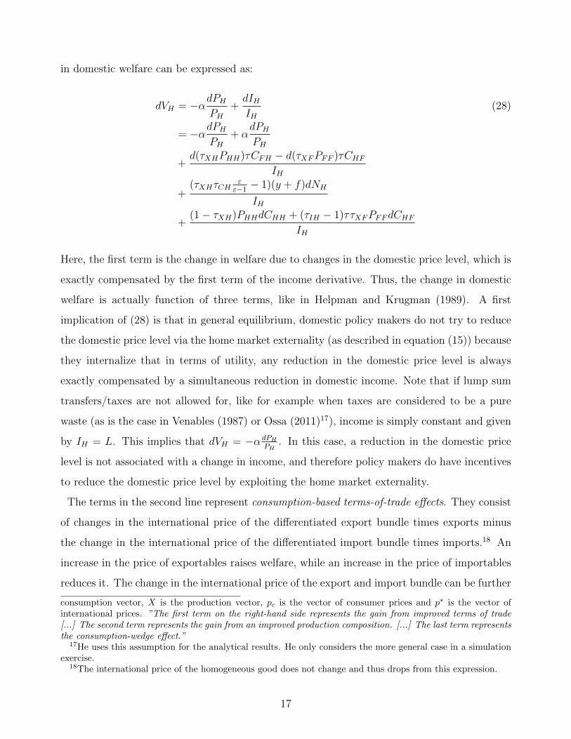
in domestic welfare can be expressed as:

dVH = −αdPHPH

+dIHIH

(28)

= −αdPHPH

+ αdPHPH

+d(τXHPHH)τCFH − d(τXFPFF )τCHF

IH

+(τXHτCH

εε−1 − 1)(y + f)dNH

IH

+(1− τXH)PHHdCHH + (τIH − 1)ττXFPFFdCHF

IH

Here, the first term is the change in welfare due to changes in the domestic price level, which is

exactly compensated by the first term of the income derivative. Thus, the change in domestic

welfare is actually function of three terms, like in Helpman and Krugman (1989). A first

implication of (28) is that in general equilibrium, domestic policy makers do not try to reduce

the domestic price level via the home market externality (as described in equation (15)) because

they internalize that in terms of utility, any reduction in the domestic price level is always

exactly compensated by a simultaneous reduction in domestic income. Note that if lump sum

transfers/taxes are not allowed for, like for example when taxes are considered to be a pure

waste (as is the case in Venables (1987) or Ossa (2011)17), income is simply constant and given

by IH = L. This implies that dVH = −αdPHPH

. In this case, a reduction in the domestic price

level is not associated with a change in income, and therefore policy makers do have incentives

to reduce the domestic price level by exploiting the home market externality.

The terms in the second line represent consumption-based terms-of-trade effects. They consist

of changes in the international price of the differentiated export bundle times exports minus

the change in the international price of the differentiated import bundle times imports.18 An

increase in the price of exportables raises welfare, while an increase in the price of importables

reduces it. The change in the international price of the export and import bundle can be further

consumption vector, X is the production vector, pc is the vector of consumer prices and p∗ is the vector ofinternational prices. ”The first term on the right-hand side represents the gain from improved terms of trade[...] The second term represents the gain from an improved production composition. [...] The last term representsthe consumption-wedge effect.”

17He uses this assumption for the analytical results. He only considers the more general case in a simulationexercise.

18The international price of the homogeneous good does not change and thus drops from this expression.

17

decomposed as:

d(τXHPHH) =ε

ε− 1N− 1ε−1

H d(τXHτCH)− τXHτCHε− 1

ε

ε− 1N− εε−1

H dNH (29)

d(τXFPFF ) =ε

ε− 1N− 1ε−1

F d(τXF τCF )− τXF τCFε− 1

ε

ε− 1N− εε−1

F dNF

Thus, consumption-based terms of trade improve directly through increases in τXH and τCH ,

which make exports more expensive, and through reductions in τXF and τCF , which make

imports cheaper. This is the traditional direct terms-of-trade effect. Moreover, consumption-

based terms of trade improve indirectly through reductions in NH and increases in NF because

they increase the international price of exports and lower the international price of imports of

one unit of the respective sub-utility. In this sense, import taxes can also have indirect terms-

of-trade effects by changing the number of varieties produced in each country. Finally, note

that an increase in NH or a reduction in NF cannot be interpreted as a home market externality

because both are welfare reducing, whereas positive welfare effects of such changes would be

required to make them interpretable as such.

The term in the third line represents what Helpman and Krugman (1989) refer to as ’gain

from an improved production composition’. We label this the production efficiency effect. It

represents the trade off between producing one more variety of the differentiated good and

giving up LH(i) = y + f units of QZH , evaluated at international prices.19 The production

efficiency effect is zero when τXHτCH = ε−1ε

, i.e., when production and/or export subsidies are

set so as to eliminate the price markup charged by domestic firms. When this is the case, there

are no efficiency gains from relocating labor from one sector to the other. In contrast – as

shown in section 3.1 – at the free trade allocation there is too little provision of differentiated

varieties and too much production of the homogenous good. In this case, the production

efficiency term equals εε−1fdNH , implying that policy makers have an incentive to induce a

reallocation of labor from the homogenous to the differentiated sector. Given that a relocation

of firms to the domestic economy will exactly achieve this goal, they have an incentive to use

trade policy to induce this outcome. However, observe that such relocation motive is no longer

present once production efficiency has been reached. Indeed, the term becomes negative if the

subsidies exceed the price markup i.e., whenever there is over-subsidizing further increasing NH

19Indeed, in equilibrium, dNH = −εfdQZH .

18

reduces welfare. This term will be crucial to understand the policy outcomes of the different

instruments.

Finally, the terms in the last line represent consumption wedges due to import or export

taxes. By generating a differences between domestic and international prices, trade taxes induce

domestic households to consume too little or too much of Foreign or domestic differentiated

goods. A tariff, for instance, renders Foreign varieties too expensive for domestic households

and generates an inefficiency by lowering CHF . Hence, as long as τIH > 1, any increase in the

Home demand for Foreign differentiated goods partially corrects for this distortion and raises

welfare. On the other hand, an export subsidy increases the demand of foreigners for Home

varieties and reduces that of domestic households. As a result, CHH is inefficiently low and as

long as τXH < 1, an increase in the domestic demand for Home differentiated goods is welfare

improving. Observe that these terms are zero when there are no trade taxes like, for example,

at the free trade allocation or when production taxes are the only instruments. In fact, in the

absence of trade taxes, domestic and international prices are equal and consumption wedges

are absent.20

4 Production Taxes

In this section we study cooperative and non-cooperative production subsidies/taxes, assuming

that they are the only available policy instruments, i.e., τIH = τIF = τXH = τXF = 1. We first

discuss cooperative production taxes and then turn to a discussion of strategic ones.

Proposition 2: Cooperative Production Subsidy. The optimal cooperative production

subsidy is set to exactly offset the price markup generated by monopolistic competition. This

subsidy implements a symmetric equilibrium with the first-best number of varieties. Formally,

(1) τCoopC = ε−1ε

and NCoop = NFB.

To gain intuition for the incentives behind such policy outcome, it is useful to express the

20Helpman and Krugman (1989) pointed out that whenever the trade tax τmj is close to one, the consumption-wedge effect is second order in size and can even be disregarded. Nonetheless, we always account for those effectsin our welfare decomposition.

19

cooperative welfare changes using (28) for both countries:

dVH + dVF =(τCH

εε−1 − 1)(y + f)dNH

IH+

(τCFεε−1 − 1)(y + f)dNF

IF(30)

where dNH = ∂NH∂τCH

dτCH + ∂NH∂τCF

dτCF and dNF = ∂NF∂τCF

dτCF + ∂NF∂τCH

dτCH . Under cooperation,

the common authority takes into account the externality produced on the other country, so

that consumption-based terms-of-trade effects exactly compensate since they are equal and of

opposite signs. Moreover, when production taxes are the only instrument, consumption wedges

are absent. Therefore, the production efficiency effect is the only driving incentive of the

cooperative policy maker. The cooperative welfare is increasing in the two subsidies (dNH > 0,

dNF > 0)21 as long as ε−1ε< τCoopC ≤ 1, and is maximized for τCoopC = ε−1

ε.

Differently, unilateral setting of production taxes does not lead to the first-best outcome due

to the consumption-based terms-of-trade externality, as formally stated in Lemma 1.

Lemma 1: Unilaterally Set Production Subsidies. The optimal unilateral deviation

entails a reduction in the production subsidy when starting from the efficient allocation. When

starting from the free trade allocation, the optimal unilateral deviation entails a production

subsidy. Formally,

(1) If τCH = τCF = ε−1ε

, ∂VH∂τCH

> 0.

(2) If τCH = τCF = 1, ∂VH∂τCH

< 0.

Using our welfare decomposition, welfare changes induced by unilateral production taxes are

given by:

dVH =d(PHH)τCFH − d(PFF )τCHF

IH+

(τCHεε−1 − 1)(y + f)dNH

IH, (31)

where dPHH and dPFF can be further decomposed as in (29), and dNH = ∂NH∂τCH

dτCH . Thus,

single-country policy makers’ actions are determined both by the consumption-based terms-of-

trade effect (first term) and the production efficiency effect (second term). There is a trade off

between these two effects: terms-of-trade effects call for a production tax which improves terms

21See Lemma A1 (1) in Appendix D for the proof of the incentives driving cooperative policy choice.

20

of trade both directly – by increasing the international price of individual varieties (direct terms-

of-trade effect) – and indirectly – by reducing the number of domestically produced varieties.

Instead, the production efficiency effect warrants a production subsidy that increases domestic

entry and brings factory gate prices down to marginal costs.22 Overall, this trade off leads to a

production subsidy which, however, is inefficiently small. Note also that any production subsidy

that is larger than the first-best level would be clearly welfare detrimental because it would

make both terms-of-trade and production efficiency effects negative. This intuition carries over

to strategically set production taxes, as stated in Proposition 3.

Proposition 3: Nash-Equilibrium Production Subsidies. In the Nash equilibrium both

countries set a production subsidy. However, this subsidy is smaller than the one needed to

implement the first-best allocation. The equilibrium number of varieties larger than in the free

trade allocation, but lower than the first-best level. Formally,

(1) τ coopC < τNashC < 1 and NFT < NNash < NFB.

Thus, single-country policy makers never over-subsidize domestic production, as would be

required if the home market externality were the dominating incentive for non-cooperative

policy choice. Instead, the trade off between production efficiency effects and terms-of-trade

effects leads policy makers to choose an inefficiently low level of production subsidies. This is an

important result, because it contradicts the standard wisdom that in the two-sector Krugman

model countries have an incentive to over-subsidize production in order to attract more firms

(Venables (1987)).

5 Import Taxes

Here, we assume that the only strategic trade policy instrument available is an import tar-

iff/subsidy. Given the results of the previous section, where we pointed out the importance of

the production efficiency effect, we study cooperative and non-cooperative import taxes under

two scenarios. In the first scenario, production subsidies have already been set in a non-strategic

fashion such as to eliminate monopolistic distortions and to implement the first-best allocation

22See Lemmata A1 (2) and A1 (3) in Appendix D for the proofs of the incentives driving unilateral deviations.

21

(i.e., τCH = τCF = ε−1ε

and production efficiency effects are absent), while in the second scenario

monopolistic distortions are present (i.e., τCH = τCF = 1). Let us first study the cooperative

policy maker’s problem.

Proposition 4: Cooperative Import Subsidy. If τCH = τCF = ε−1ε

, the cooperative policy

maker refrains from using taxes on imports and the number of varieties equals the first-best

level. If τCH = τCF = 1, the cooperative policy maker finds it optimal to subsidize imports.

The number of varieties is larger than in the free trade allocation, but remains lower than the

first-best level. Formally,


, then τCoopI = 1 and NCoop = NFB.

(2) If τCH = τCF = 1, then ε−1ε< τCoopI < 1 and NFT < NCoop < NFB.

Again, we can use (28) for both countries to decompose the cooperative welfare change:

dVH + dVF =(τCH

εε−1 − 1)(y + f)dNH

IH+

(τCFεε−1 − 1)(y + f)dNF

IF(32)

+(τIH − 1)τPFFdCHF

IH+

(τIF − 1)τPHHdCFHIF

,

where dNH = ∂NH∂τIH

dτIH + ∂NH∂τIF

dτIF , dNF = ∂NF∂τIF

dτIF + ∂NF∂τIH

dτIH , dCHF = ∂CHF∂τIH

dτIH + ∂CHF∂τIF

dτIF

and dCFH = ∂CFH∂τIF

dτIF + ∂CFH∂τIH

dτIH . Thus, the cooperative welfare change can be decomposed

into the production efficiency effect (first line) and consumption wedges (second line). Observe

that when production subsidies are set at the first-best level, τCH = τCF = ε−1ε

, the terms related

to production efficiency are zero. In this case, setting τIH = τIF = 1, also makes consumption

wedges disappear and this solves the cooperative import policy problem. Differently, when

production subsidies are not available, i.e., τCH = τCF = 1, the production efficiency effect is

positive and an increase in domestic and foreign varieties (dNH > 0, dNF > 0) increases welfare.

To achieve that, the cooperative policy maker has an incentive to implement symmetric import

subsidies in both countries, which increase the demand for imported varieties and trigger entry

into the differentiated sectors in both countries. However, this comes at the cost of creating

wedges: the domestic price of imported varieties becomes lower than its international price

and this tilts the consumption allocation inefficiently towards imported varieties. This can be

clearly seen from the above formula. When τIH = τIF < 1, the terms (τIj − 1) are negative so

22

that an increase in consumption of imported varieties induced by import subsidies (dCHF > 0,

dCFH > 0) reduces welfare.23 As a result, when only import taxes are available, production

and consumption inefficiencies cannot be eliminated simultaneously and the cooperative import

subsidy implements a second-best allocation.

Once we move to the case of non-cooperation, trade policy outcomes crucially depend on

whether production efficiency effects are present, as stated formally by Lemma 2 for the case

of unilateral import taxes.

Lemma 2: Unilaterally Set Import Tariffs/Subsidies. Let τIH = τIF = 1. The opti-

mal unilateral deviation entails an import subsidy when starting from the first-best allocation

implemented by a production subsidy, and an import tariff when starting from the free trade

allocation. Formally,


, then ∂VH∂τIH

< 0.

(2) If τCH = τCF = 1, then ∂VH∂τIH

> 0.

To understand this difference in import policy choice, we use once more our welfare decompo-

sition (28):

dVH =d(PHH)τCFH − d(PFF )τCHF

IH+

(τCHεε−1 − 1)(y + f)dNH

IH(33)

where dPHH and dPFF can be further decomposed as in (29) and dNH = ∂NH∂τIH

dτIH . Consump-

tion wedges are absent since τIH = τIF = 1 and the change in domestic welfare induced by

changes in unilateral import taxes is given by consumption-based terms-of-trade effects (first

term) and production efficiency effects (second term). When τCH = ε−1ε

, there are no produc-

tion efficiency effects and import taxes have only indirect consumption-based terms-of-trade

effects through their effect on the number of varieties produced in each country. The optimal

unilateral policy choice is an import subsidy which shifts domestic demand towards imported

varieties. This triggers exit of firms from the domestic differentiated sector and entry in Foreign,

thereby indirectly improving domestic consumption-based terms of trade.

In contrast, at the free trade allocation with τCH = τCF = 1, both consumption-based terms-

of-trade effects and production efficiency effects are present. While the first one calls for an

23See Lemma A2 (1) in Appendix E for the proof of the incentives driving cooperative policy choice.

23

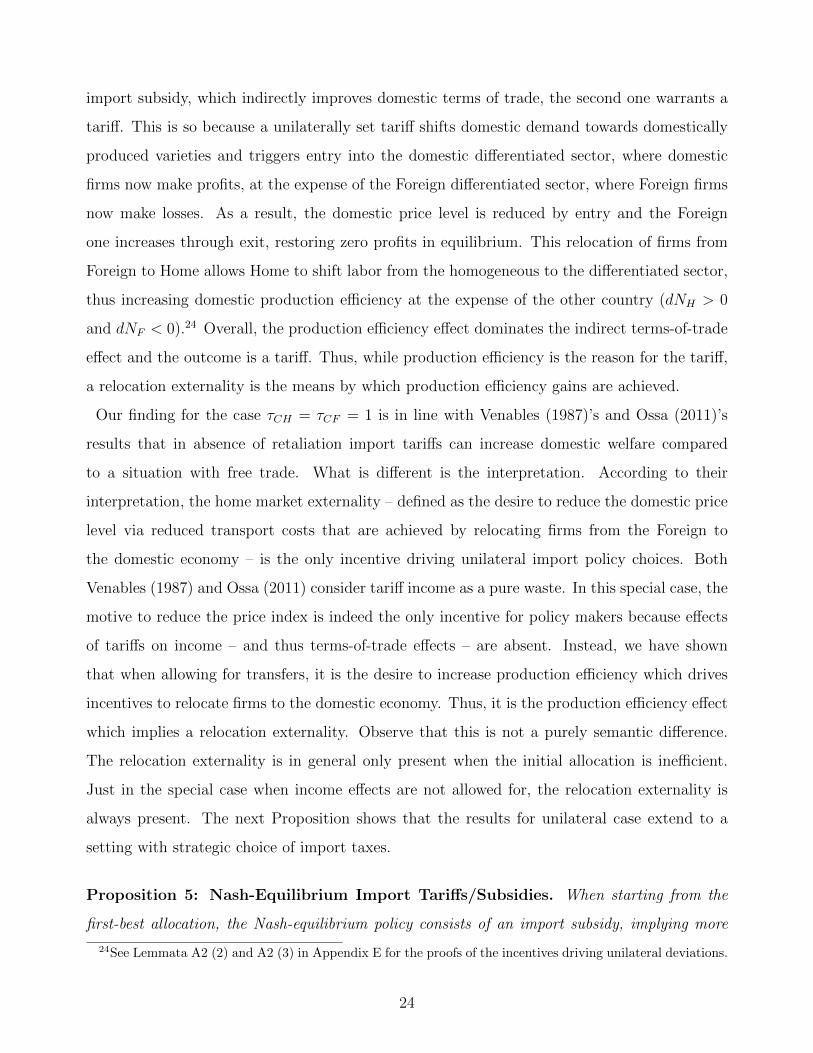
import subsidy, which indirectly improves domestic terms of trade, the second one warrants a

tariff. This is so because a unilaterally set tariff shifts domestic demand towards domestically

produced varieties and triggers entry into the domestic differentiated sector, where domestic

firms now make profits, at the expense of the Foreign differentiated sector, where Foreign firms

now make losses. As a result, the domestic price level is reduced by entry and the Foreign

one increases through exit, restoring zero profits in equilibrium. This relocation of firms from

Foreign to Home allows Home to shift labor from the homogeneous to the differentiated sector,

thus increasing domestic production efficiency at the expense of the other country (dNH > 0

and dNF < 0).24 Overall, the production efficiency effect dominates the indirect terms-of-trade

effect and the outcome is a tariff. Thus, while production efficiency is the reason for the tariff,

a relocation externality is the means by which production efficiency gains are achieved.

Our finding for the case τCH = τCF = 1 is in line with Venables (1987)’s and Ossa (2011)’s

results that in absence of retaliation import tariffs can increase domestic welfare compared

to a situation with free trade. What is different is the interpretation. According to their

interpretation, the home market externality – defined as the desire to reduce the domestic price

level via reduced transport costs that are achieved by relocating firms from the Foreign to

the domestic economy – is the only incentive driving unilateral import policy choices. Both

Venables (1987) and Ossa (2011) consider tariff income as a pure waste. In this special case, the

motive to reduce the price index is indeed the only incentive for policy makers because effects

of tariffs on income – and thus terms-of-trade effects – are absent. Instead, we have shown

that when allowing for transfers, it is the desire to increase production efficiency which drives

incentives to relocate firms to the domestic economy. Thus, it is the production efficiency effect

which implies a relocation externality. Observe that this is not a purely semantic difference.

The relocation externality is in general only present when the initial allocation is inefficient.

Just in the special case when income effects are not allowed for, the relocation externality is

always present. The next Proposition shows that the results for unilateral case extend to a

setting with strategic choice of import taxes.

Proposition 5: Nash-Equilibrium Import Tariffs/Subsidies. When starting from the

first-best allocation, the Nash-equilibrium policy consists of an import subsidy, implying more

24See Lemmata A2 (2) and A2 (3) in Appendix E for the proofs of the incentives driving unilateral deviations.

24

varieties than the first-best allocation. In contrast, when starting from the free trade alloca-

tion, the Nash-equilibrium entails a tariff, implying less varieties than the free trade allocation.

Formally,


, then τNashI < 1 and NFT < NFB < NNash.

(2) If τCH = τCF = 1, then there exists a τNashI > 1 such that NNash < NFT < NFB.

First, note that on top of the production efficiency effect and terms-of-trade effect described

in Lemma 2, in the Nash equilibrium import taxes also generate consumption wedges. How-

ever, the Nash outcomes are exactly the ones we would have expected from the incentives for

unilateral deviations. When starting from the first-best allocation, the optimal Nash policy is

an import subsidy. The intuition follows from the incentives for unilateral policies: the import

subsidy aims at improving consumption-based domestic terms of trade indirectly by reducing

the number of domestic firms. Yet, in equilibrium no country reaches this aim and entry in-

creases beyond efficiency. According to the second part of Proposition 5, when there is no

correction of the monopolistic distortion, non-cooperative trade policy brings about a positive

tariff. From Lemma 2 (2) we know that the production efficiency effect is behind the choice

of setting a unilateral import tariff. However, in the Nash equilibrium no country manages to

relocate firms to its domestic market thereby failing to increase production efficiency. Instead,

tariffs reduce the world equilibrium number of varieties.

6 Export Taxes

In this section, we consider export subsidies/taxes as the only strategic trade policy instrument

available. In line with the previous analysis, we study cooperative and Nash policies under two

scenarios. In the first one production subsidies have been set such as to implement the first-best

allocation (i.e., τCH = τCF = ε−1ε

), while in the second scenario monopolistic distortions have

not been corrected (i.e., τCH = τCF = 1).

Proposition 6: Cooperative Export Subsidy. If τCH = τCF = ε−1ε

, the cooperative policy

maker refrains from using taxes on exports and the number of varieties equals the first-best

level. If τCH = τCF = 1, the cooperative policy maker finds it optimal to subsidize exports.

25

The number of varieties is larger than in the free trade allocation, but remains lower than the

first-best level. Formally,


, then τCoopX = 1 and NCoop = NFB.

(2) If τCH = τCF = 1, then τCoopX < 1 and NFT < NCoop < NFB.

Incentives to set export subsidies can again be best understood using the welfare decomposition

(28), which now becomes

dVH + dVF =(τXHτCH

εε−1 − 1)(y + f)dNH

IH+

(τXF τCFεε−1 − 1)(y + f)dNF

IF(34)

+(1− τXH)PHHdCHH

IH+

(1− τXF )PFFdCFFIF

,

where dNH = ∂NH∂τXH

dτXH + ∂NH∂τXF

dτXF , dNF = ∂NF∂τXH

dτXH + ∂NF∂τXF

dτXF , dCHH = ∂CHH∂τXH

dτXH +

∂CHH∂τXF

dτXF and dCFF = ∂CFF∂τXH

dτXH + ∂CFF∂τXF

dτXF . Terms in the first line of (34) are production

efficiency effects while terms in the second line are consumption wedges. When production

subsidies are set at their first-best level, i.e., τCH = τCF = ε−1ε

, it is easy to see that both

production efficiency effects and consumption wedges are zero if τXH = τXF = 1. In contrast,

when no production subsidies are available i.e., τCH = τCF = 1, production efficiency can be

improved by setting export subsidies in both countries, which increase demand for differentiated

varieties and trigger entry into the differentiated sectors (dNH > 0, dNF > 0).25 However, this

comes at the cost of creating consumption wedges. As for the case of import subsidies, this

trade off leads to a second-best outcome, which improves upon the free trade allocation but

does not eliminate all distortions. We now turn to a discussion of non-cooperative export taxes.

Lemma 3: Unilaterally Set Export Taxes/Subsidies. Let τXH = τXF = 1. The optimal

unilateral deviation entails an export tax when starting from the first-best allocation implemented

by a production subsidy, and an export subsidy when starting from the free trade allocation.

Formally,


, then ∂VH∂τXH

> 0.

(2) If τCH = τCF = 1, then ∂VH∂τXH

< 0.

25See Lemma A3 (1) in Appendix F for the proof of the incentives driving cooperative policy choices.

26

Once again, we use our welfare decomposition (28):

dVH =d(τXHPHH)τCFH − d(τXFPFF )τCHF

IH+

(τXHτCHεε−1 − 1)(y + f)dNH

IH(35)

where d(τXHPHH) and d(τXFPFF ) can be further decomposed as in (29) and dNH = ∂NH∂τXH

dτXH .

The first term in (35) is the consumption based terms-of-trade effect, while the second term is

the production efficiency effect. When τCH = ε−1ε

, production efficiency effects are absent as

long as τXH = 1. However, policy makers have incentives to unilaterally deviate by setting a

small export tax. Such an export tax indeed improves domestic terms of trade both directly,

through an increase in the international price of domestically produced varieties, and indirectly,

via a reduction in the number of domestic firms and an increase in the number of foreign ones.

Differently, at the free trade allocation with τCH = τCF = 1 production efficiency effects

are present and call for an export subsidy.26 Overall, negative terms-of-trade effects of an

export subsidy are out-weighted by production efficiency gains. A small export subsidy triggers

entry into the domestic differentiated sector, thereby improving domestic production efficiency.

This creates a relocation externality, since it induces exit of firms from Foreign. However,

the relocation effect is just the means to increase domestic production efficiency. The next

Proposition shows that the results on unilateral changes extend to a setup with strategic choice

of the export policy instrument.

Proposition 7: Nash-Equilibrium Export Taxes/Subsidies. When starting from the

first-best allocation, the Nash-equilibrium policy consists of an export tax, implying less varieties

than the first-best allocation. In contrast, when starting from the free trade allocation, the Nash

equilibrium entails an export subsidy, implying more varieties than the free trade allocation.

Formally,


, then τNashX > 1 and NNash < NFB.

(2) If τCH = τCF = 1, then τNashX < 1 and NFT < NNash < NFB.

Proposition 7 makes it clear that in this case too, the outcome of the policy game depends

crucially on whether the initial allocation is (in)efficient. When starting from the free trade

26See Lemmata A3 (2) and A3 (3) in Appendix F for the proofs of the incentives driving unilateral deviations.

27

allocation the optimal Nash policy is an export subsidy, whereas when starting from the first-

best allocation the optimal non-cooperative policy is an export tax. Again, even though the

export taxes/subsidies will induce consumption wedges in the Nash equilibrium, the intuition is

the one provided for the unilateral policy choice. If the initial allocation is efficient consumption-

based terms-of-trade effects call for an export tax, but in the Nash outcome both countries fail

to improve their terms of trade. If instead the initial allocation is inefficient, the production

efficiency effect prevails and the policy makers choose an export subsidy.

7 Simultaneous Policy Choice

Finally, in this section we allow for simultaneous choice of all three policy instruments.

Proposition 8: Cooperative Policy Instruments. The cooperative policy maker sets the

first-best level of production subsidies and chooses the trade taxes such that τCoopI · τCoopX = 1.

The number of varieties equals the first-best level.


, τCoopI · τCoopX = 1 and NCoop = NFB.

This result is straightforward: the cooperative policy maker uses the production subsidy

to reach the first-best allocation and either refrains from using trade instruments (τCoopI =

τCoopX = 1), or uses them in a way that does not create consumption wedges (τCoopI · τCoopX = 1).

Differently, non-cooperative policy makers intend to manipulate international prices in their

favor.

Proposition 9: Nash-Equilibrium Policy Instruments. The Nash-equilibrium policy con-

sists of the first-best level of production subsidies, and inefficient import subsidies and export

taxes. Formally,

(1) τNashC = τCoopC = ε−1ε

, τNashI < 1 and τNashX > 1.

The result that production subsidies are set so as to completely offset monopolistic distortions

is an application of the principle of targeting in public economics (Dixit (1985)). It states that

an externality or distortion is best countered with a tax instrument that acts directly on the

appropriate margin. Only when such an instrument is not available, trade policy can be used

28

as a second-best policy. This confirms that the inefficiency of the market allocation crucially

affects policy makers’ incentives to set import tariffs or export subsidies. Once uncoordinated

policy makers have all the necessary instruments to eliminate these distortions, the only motive

to set trade policy is the incentive to improve domestic terms of trade. Export taxes achieve this

directly by increasing the international price of domestic varieties and indirectly by reducing

the number of domestically produced varieties, while import tariffs only impact on terms of

trade through this indirect channel.27 Moreover, this finding also strengthens the results from

the previous sections, where first-best production subsidies were set in a non-strategic fashion

and confirms our approach to isolate efficiency considerations from other motives to set trade

policy.

Finally, note that our finding that terms-of-trade effects are the dominating motive for trade

policy in the Krugman model is closely related to Bagwell and Staiger (2009) who derive a very

similar result for the case where countries can set import and export taxes simultaneously but

do not have access to production taxes. They find that countries’ best response to an import

tariff would be to set an offsetting export subsidy, and thus the relocation motive is not present

in the incentives that determine Nash-equilibrium policy choice. Instead, only terms-of-trade

effects survive. This is in line with our result that when additionally production subsidies

are available, they will be set to the first-best level while the trade instruments are driven by

terms-of-trade effects.

8 Conclusions

In this paper we have studied cooperative, unilateral and strategic trade policies in a two-sector

Krugman (1980) model of intra-industry trade, considering production, import and export taxes

as trade policy instruments. It is common wisdom that in this model non-cooperative trade

policies are set in order to try to agglomerate firms in the domestic economy, which reduces

transport costs for domestic consumers and thus the domestic price level (home market effect).

Contrary to the results of the previous literature, we show that in this model the home market

effect is not a motive for non-cooperative trade policy choices. Instead, they are driven by pro-

27It is easy to show that using both trade instruments unilaterally improves terms of trade by more thanwhen relying only on a single one.

29

duction efficiency considerations, on the one hand, and by consumption-based terms-of-trade

effects on the other. Indeed, due to monopolistic competition, in the free trade equilibrium

there are too few firms in the differentiated sector and this affects policy makers’ incentives

in a crucial way. Thus, when production taxes are available, non-cooperative policy makers

increase production efficiency by setting production subsidies. However, due to terms-of-trade

effects these subsidies are lower than the cooperatively set ones. When only import (export)

tax instruments are available, non-cooperative policy makers use tariffs (export subsidies) to

increase production efficiency, thereby imposing a relocation externality on the other country.

However, once monopolistic distortions have been offset by appropriate production subsidies,

results turn around: policy makers set import subsidies (export taxes), which improve domes-

tic consumption-based terms of trade. Finally, when policy makers can set all three policy

instruments simultaneously, they choose to set production subsidies, which exactly offset mo-

nopolistic distortions. Moreover, they set import subsidies and export taxes, both of which aim

at improving domestic terms of trade. The implications of our findings are important: also in

the Krugman (1980) model, terms-of-trade externalities remain the only reason why countries

need to sign trade agreements.

References

Bagwell, Kyle and Robert W. Staiger, “An Economic Theory of GATT,” American Eco-

nomic Review, 1999, 89 (1), 215–248.

and , “Delocation and Trade Agreements in Imperfectly Competitive Markets,” NBER

working paper, 2009, 15444.

Corsetti, Giancarlo and Paolo Pesenti, “Welfare and Macroeconomic Interdependence,”

Quarterly Journal of Economics, 2001, 116, 421–445.

Dixit, Avinash K., “Tax policy in Open Economies,” in Allan. J. Auerbach and Martin

Feldstein, eds., Handbook of Public Economics, Vol. 1, Elsevier, 1985.

and Joseph E. Stiglitz, “Monopolistic Competition and Optimum Product Diversity,”

American Economic Review, 1977, 67 (3), 297–308.

30

Epifani, Paolo and Gino Gancia, “Openness, Government Size and the Terms of Trade,”

Review of Economic Studies, 2009, 76, 629–668.

Gros, Daniel, “A Note on the Optimal Tariff Retaliation and the Welfare Loss from Tariff

Wars in a Framework with Intra-Industry Trade,” Journal of International Economics, 1987,

23 (3-4), 357–367.

Grossman, Gene M. and Elhanan Helpman, “Trade Wars and Trade Talks,” Journal of

Political Economy, 1985, 103, 675–708.

Helpman, Elhanan and Paul Krugman, Trade Policy and Market Structure, MIT Press,

1989.

Johnson, Harry G., “Optimum Tariffs and Retaliation,” Review of Economic Studies, 1953-

1954, 21 (2), 142–153.

Krugman, Paul, “Scale Economics, Product Differentiation, and Pattern of Trade,” American

Economic Review, 1980, 70 (5), 950–959.

Ossa, Ralph, “A ’New Trade’ Theory of GATT/WTO Negotiations,” Journal of Political

Economy, 2011, 119 (1), 122–152.

Venables, Anthony, “Trade and Trade Policy with Differentiated Products: A

Chamberlinian-Ricardian Model,” The Economic Journal, 1987, 97 (387), 700–717.

WTO, World Trade Report 2006, World Trade Organization, 2006.

31

APPENDIX

A Equilibrium

A.1 Equilibrium Allocation and Prices

Substituting the optimal pricing rules (11) and (12) into the definition of Home (6) (and Foreign)aggregate price indices we obtain:

PH =ε

ε− 1

[NHτ

1−εCH +NF (τIHτXF ττCF )1−ε

] 11−ε PF =

ε

ε− 1

[NF τ

1−εCF +NH (τIF τXHττCH)1−ε

] 11−ε

(36)

Combining the market clearing condition (18) with the analogous one for Foreign and substi-tuting out the expressions for the prices (36), gives:

CH =fP−εH (ε− 1)

(εε−1

) ετ ε[−ττ εCF + (ττCHτIF τXH)ε](τIHτXF )ε

τ 2ε(τIF τXHτIHτXF )ε − τ 2(37)

CF =fP−εF (ε− 1)

(εε−1

) ετ ε[−ττ εCH + (ττCF τIHτXF )ε](τIF τXH)ε

τ 2ε(τIF τXHτIF τXF )ε − τ 2(38)

Using the trade balance condition (21), the labor market clearing condition (20), the equivalentequations for Foreign, and the expressions for CH , CF , PH and PF just derived, we obtain thefollowing system of equations in NH and NF :

A1HNH + A2HNF − L = 0 (39)

A2FNH + A1FNF − L = 0 (40)

The solution to this system is:

NH =L(A2H − A1F )

A2FA2H − A1HA1F

NF =L(A2F − A1H)

A2FA2H − A1HA1F

(41)

where:

A1H =fετ−εCHτ

2ε(τCHτIHτIF τXHτXF )ε(α + (1− α)τCH)

α(τ 2ε(τIHτIF τXHτXF )ε − τ 2)(42)

+fετ−εCHτ [αττ εCH(τCHτXH − 1)− τCH(ττCF τIHτXF )ε(1− α + ατXH)]

α(τ 2ε(τIHτIF τXHτXF )ε − τ 2)

A2H =fεττXF τ

1−εCF (−α− (1− α)τIH)[ττ εCF − (ττCHτIF τXH)ε]


32

A1F =fετ−εCF τ

2ε(τCF τIHτIF τXτXF )ε(α + (1− α)τCF )


+fετ−εCF τ [αττ εCF (τCF τXF − 1)− τCF (ττCHτIF τXH)ε(1− α + ατXF )]

α(τ 2ε(τIHτIF τXHτXF )ε − τ 2)

A2F =fεττXHτ

1−εCH (−α− (1− α)τIF )[ττ εCH − (ττCF τIHτXF )ε]


A.2 Free Trade Allocation

Let τCH = τCF = τIH = τIF = τXH = τXF = 1. Then (41) simplifies to:

NH = NF =αL

εf≡ NFT (46)

B The Planner’s Problem

Proposition 1: First-Best Allocation. The first-best allocation entails the same firm sizebut more varieties than the free trade allocation. Formally,

(1) yFB = f(ε− 1) = yFT and NFB = αL(ε−1+α)f > NFT = αL

εf.

Proof of Proposition 1.The Lagrangian for the planner’s problem is:

L =

[∫ NH

0cHH(i)

ε−1

ε di+

∫ NF

0cHF (i)

ε−1

ε di

] εα

ε−1

Z1−αH +

[∫ NF

0cFH(i)

ε−1

ε di+

∫ NF

0cFF (i)

ε−1

ε di

] εα

ε−1

Z1−αF

+

∫ NH

0λ1(i)[LCH(i)− f − cHH(i)− τcFH(i)]di+

∫ NF

0λ2(i)[LCF (i)− f − cFF (i)− τcHF (i)]di

+ λ3[LH + LF −∫ NH

0LCH(i)di−

∫ NF

0LCF (i)di− ZH − ZF ]

The first-order conditions are:

∂L∂cHH(i)

= 0 : αCαH

[∫ NH

0

cHH(i)ε−1ε di+

∫ NF

0

cHF (i)ε−1ε di

]−1Z1−αH cHH(i)

−1ε = λ1(i) (47)

∂L∂cHF (i)

= 0 : αCαH

[∫ NH

0

cHH(i)ε−1ε di+

∫ NF

0

cHF (i)ε−1ε di

]−1Z1−αH cHF (i)

−1ε = τλ2(i) (48)

∂L∂ZH

= 0 : (1− α)CαHZ

−αH = λ3 (49)

33

∂L∂LCH(i)

= 0 : λ1(i) = λ3 (50)

∂L∂NH

= 0 :αε

ε− 1

{CαHZ

1−αH

[∫ NH

0

cHH(i)ε−1ε di+

∫ NF

0

cHF (i)ε−1ε di

]−1cHH(NH)

ε−1ε +

CαFZ

1−αF

[∫ NH

0

cFH(i)ε−1ε di+

∫ NF

0

cFF (i)ε−1ε di

]−1cFH(NH)

ε−1ε

}= λ3LCH(NH),

(51)

where in the last condition we have already used the fact that λ1(NH)[LCH(NH)−f−cHH(NH)−τcFH(NH)] = 0.The first-order conditions with respect to Foreign variables are completely symmetric and arethus omitted for the sake of space. By imposing symmetry we find λ1(i) = λ2(i). Combining(47) and (48) we obtain:

cHF (i) = cHH(i)τ−ε (52)

Combining (47), (50) and (51) we get that:

ε

ε− 1[cHH(i)

ε−1ε + cHF (i)

ε−1ε ] = LCH(i)cHH(i)

1ε (53)

Combining (52) and (53), we obtain:

cHH(i) =ε

ε− 1[1 + τ 1−ε]−1 (54)

Substituting the expression for cHH(i) and cHF (i) into the resource condition for domesticvarieties LCH(i) = f+cHH(i)+τcFH(i), we get LCH(i) = εf and using the production functionyH(i) = LCH(i) − f we obtain yFB = (ε − 1)f . Moreover, cFBHH(i) = (ε − 1)f [1 + τ 1−ε]−1 andcFBHF (i) = (ε− 1)fτ−ε[1 + τ 1−ε]−1.

Using the resource condition for ZH , we get ZH = L − NHεf . Finally, combining (47), (49)and (50):

(1− α)Cε−1ε

H = αZHcHH(i)−1ε (55)

Substituting the expressions for ZH , CH , cFBHH(i) and cFBHF (i) into (55), we can solve for NH =NF ≡ NFB = αL

f(ε+α−1) .

34

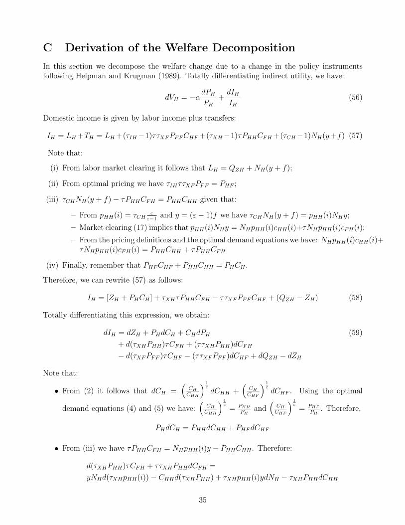
C Derivation of the Welfare Decomposition

In this section we decompose the welfare change due to a change in the policy instrumentsfollowing Helpman and Krugman (1989). Totally differentiating indirect utility, we have:

dVH = −αdPHPH

+dIHIH

(56)

Domestic income is given by labor income plus transfers:

IH = LH +TH = LH +(τIH−1)ττXFPFFCHF +(τXH−1)τPHHCFH +(τCH−1)NH(y+f) (57)

Note that:

(i) From labor market clearing it follows that LH = QZH +NH(y + f);

(ii) From optimal pricing we have τIHττXFPFF = PHF ;

(iii) τCHNH(y + f)− τPHHCFH = PHHCHH given that:

– From pHH(i) = τCHεε−1 and y = (ε− 1)f we have τCHNH(y + f) = pHH(i)NHy;

– Market clearing (17) implies that pHH(i)NHy = NHpHH(i)cHH(i)+τNHpHH(i)cFH(i);

– From the pricing definitions and the optimal demand equations we have: NHpHH(i)cHH(i)+τNHpHH(i)cFH(i) = PHHCHH + τPHHCFH

(iv) Finally, remember that PHFCHF + PHHCHH = PHCH .

Therefore, we can rewrite (57) as follows:

IH = [ZH + PHCH ] + τXHτPHHCFH − ττXFPFFCHF + (QZH − ZH) (58)

Totally differentiating this expression, we obtain:

dIH = dZH + PHdCH + CHdPH (59)

+ d(τXHPHH)τCFH + (ττXHPHH)dCFH

− d(τXFPFF )τCHF − (ττXFPFF )dCHF + dQZH − dZH

Note that:

• From (2) it follows that dCH =(

CHCHH

) 1εdCHH +

(CHCHF

) 1εdCHF . Using the optimal

demand equations (4) and (5) we have:(

CHCHH

) 1ε

= PHHPH

and(

CHCHF

) 1ε

= PHFPH

. Therefore,

PHdCH = PHHdCHH + PHFdCHF

• From (iii) we have τPHHCFH = NHpHH(i)y − PHHCHH . Therefore:

d(τXHPHH)τCFH + ττXHPHHdCFH =

yNHd(τXHpHH(i))− CHHd(τXHPHH) + τXHpHH(i)ydNH − τXHPHHdCHH

35

Note also that from (8) and (9) we have −αdPHPH

= −CHIHdPH . Therefore, indirect utility is given

by:

dVH = −CHIH

dPH +CHIH

dPH +yNHd(τXHpHH(i))− d(τXHPHH)CHH − d(τXFPFF )τCHF

IH

+dQZH + τXHpHH(i)ydNH

IH+

(1− τXH)PHHdCHH + (τIH − 1)ττXFPFFdCHFIH

(60)

From (iii) and the fact that pHH(i) = PHHN1ε−1

H we have CHH = yNεε−1

H − τCFH . Using this

and observing that Nεε−1

H d(τXHPHH) = NHd(τXHpHH(i)) + 11−εpHH(i)τXHdNH , we can write

(60) as:

dVH = −CHIH

dPH +CHIH

dPH (61)

+d(τXHPHH)τCFH − d(τXFPFF )τCHF

IH

+dQZH + τXHpHH(i)ydNH + τXHpHH(i)y

(ε−1) dNH

IH

+(1− τXH)PHHdCHH + (τIH − 1)ττXFPFFdCHF

IH

Equation (28) follows immediately from this expression by observing that QZH = L−NHεf ,y = (ε− 1)f and pHH(i) = τCH

εε−1 . Thus, the production efficiency effect can be rewritten as:

dQZH + τXHpHH(i)yε

ε− 1dNH =

(τXHτCH

ε

ε− 1− 1

)(y + f)dNH (62)

D Production Taxes

In this section we set τIH = τIF = τXH = τXF = 1 and we prove the propositions and thelemmata of section 4.

Lemma A1: Policy Incentives for Production Subsidies. Assume ε−1ε≤ τCH = τCF ≤

1. Then, when there is a symmetric increase in the production subsidies in Home and Foreign,production efficiency effects are positive. At the same time, when there is an unilateral increasein the production subsidy in Home, the production efficiency effect is positive in the domesticeconomy and negative in the foreign one, while domestic terms-of-trade effects are negative.Formally,

(1) Let dτCH = dτCF < 0, then(τCH

εε−1−1)(y+f)dNHIH

=(τCF

εε−1−1)(y+f)dNFIF

> 0.

(2) Let dτCH < 0,(τCH

εε−1−1)(y+f)dNHIH

> 0,(τCF

εε−1−1)(y+f)dNFIF

< 0 and dPHHτCFH−dPFF τCHFIH

<0.

36

Proof of Lemma A1.

(1) By imposing symmetry we obtain:

dNH = dNF =∂NH

∂τCHdτCH+

∂NH

∂τCFdτCF =

(∂NH

∂τCH+∂NF

∂τCH

)dτCH =

(∂NH

∂τCF+∂NF

∂τCF

)dτCF

Then, (1) follows from the fact that if τCH = τCF = τC ≤ 1:

∂NH

∂τCH+∂NF

∂τCH=∂NH

∂τCF+∂NF

∂τCF= − L(1− α)α

fε[α− (α− 1)τC ]2< 0 (63)

which implies that dNH > 0 and dNF > 0 as long as dτCH < 0 and dτCF < 0.

(2) Observe that for ε−1ε≤ τCH = τCF ≤ 1, we have that (τCH

εε−1 − 1)(y + f) > 0. Hence

the domestic (Foreign) production efficiency effect has the same sign as dNH (dNF ).Moreover, once we impose symmetry, terms of trade effects in (31) can be written as:(

εε−1N

− 1ε−1

H dτCH − τCHε−1

εε−1N

− εε−1

H dNH + τCFε−1

εε−1N

− εε−1

F dNF

)τCHF

IH(64)

Thus, to prove (2) it suffices to show that as long as dτC < 0, dNH = ∂NH∂τCH

dτCH > 0 and

dNF = ∂NF∂τCH

dτCH < 0. This follows from the fact that if τCH = τCF = τC ≤ 1, then:

∂NH

∂τCH=

Lα [τ 2 (α2 + (1− α2) τC) + τ ε+1 (2(1− α)(ε− 1)τC + α(2ε− 1)) + (1− α)τ 2ε ((1− α)τC + α)]

fε (τ ε − τ) [α− (α− 1)τC ]2 [α(τ + τ ε)(τC − 1)− τC(τ ε − τ)]< 0

∂NF

∂τCH=

Lατ [α(τ ε − τ) + τ ε (2(α− 1)ετC − 2αε)]

fε (τ ε − τ) [α− (α− 1)τC ]2 [α(τ + τ ε)(τC − 1)− τC(τ ε − τ)]> 0

In fact, the denominator of both expressions is negative whenever τC ≤ 1. The numeratorof the first expression is always positive being the sum of only positive terms. For the

numerator of the second expression to be positive we would need τC <α(1−τ1−ε−2ε)

2(1−α)ε , whichis not possible given that τC ≥ 0 by definition.

Proposition 2: Cooperative Production Subsidy. The optimal cooperative productionsubsidy is set to exactly offset the price markup generated by monopolistic competition. Thissubsidy implements a symmetric equilibrium with the first-best number of varieties. Formally,


and NCoop = NFB.

37

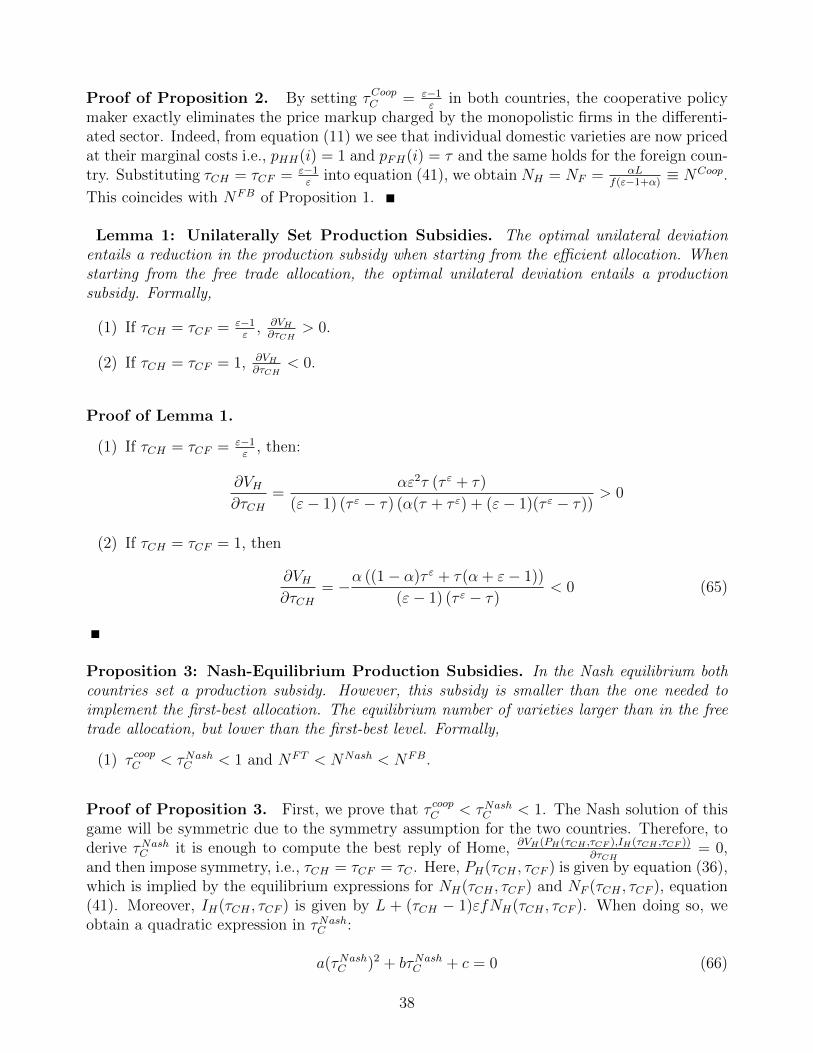
Proof of Proposition 2. By setting τCoopC = ε−1ε

in both countries, the cooperative policymaker exactly eliminates the price markup charged by the monopolistic firms in the differenti-ated sector. Indeed, from equation (11) we see that individual domestic varieties are now pricedat their marginal costs i.e., pHH(i) = 1 and pFH(i) = τ and the same holds for the foreign coun-try. Substituting τCH = τCF = ε−1

εinto equation (41), we obtain NH = NF = αL

f(ε−1+α) ≡ NCoop.

This coincides with NFB of Proposition 1.

Lemma 1: Unilaterally Set Production Subsidies. The optimal unilateral deviationentails a reduction in the production subsidy when starting from the efficient allocation. Whenstarting from the free trade allocation, the optimal unilateral deviation entails a productionsubsidy. Formally,


, ∂VH∂τCH

> 0.

(2) If τCH = τCF = 1, ∂VH∂τCH

< 0.

Proof of Lemma 1.


, then:

∂VH∂τCH

=αε2τ (τ ε + τ)

(ε− 1) (τ ε − τ) (α(τ + τ ε) + (ε− 1)(τ ε − τ))> 0

(2) If τCH = τCF = 1, then

∂VH∂τCH

= −α ((1− α)τ ε + τ(α + ε− 1))

(ε− 1) (τ ε − τ)< 0 (65)

Proposition 3: Nash-Equilibrium Production Subsidies. In the Nash equilibrium bothcountries set a production subsidy. However, this subsidy is smaller than the one needed toimplement the first-best allocation. The equilibrium number of varieties larger than in the freetrade allocation, but lower than the first-best level. Formally,

(1) τ coopC < τNashC < 1 and NFT < NNash < NFB.

Proof of Proposition 3. First, we prove that τ coopC < τNashC < 1. The Nash solution of thisgame will be symmetric due to the symmetry assumption for the two countries. Therefore, toderive τNashC it is enough to compute the best reply of Home, ∂VH(PH(τCH ,τCF ),IH(τCH ,τCF ))

∂τCH= 0,

and then impose symmetry, i.e., τCH = τCF = τC . Here, PH(τCH , τCF ) is given by equation (36),which is implied by the equilibrium expressions for NH(τCH , τCF ) and NF (τCH , τCF ), equation(41). Moreover, IH(τCH , τCF ) is given by L + (τCH − 1)εfNH(τCH , τCF ). When doing so, weobtain a quadratic expression in τNashC :

a(τNashC )2 + bτNashC + c = 0 (66)

38

where a ≡ α(1−α)ετ ε[(3− 2ε−α)τ − (1−α)τ ε], b ≡ α[(ε− 1 +α)τ 2 + (1−α)(ε− 1−α(2ε−1))τ 2ε + (2ε− 2 + α)(ε− 1− α(2ε− 1))τ 1+ε] and c ≡ α2(ε− 1)τ ε((2ε− 1 + α)τ + (1− α)τ ε).Note that a < 0 and c > 0. To prove that a < 0 it suffices to see that:

(i) τ ε > τ ∀ε > 1 and ∀τ > 1;

(ii) 1− α > 3− 2ε− α ∀ε > 1.

Hence, (66) has two real solutions, one positive and one negative ∀ε > 1, α ∈ (0, 1) and τ > 1.Then, since τNashC ∈ [0,∞), (66) implies that the Nash solution always exists and is unique. Asa consequence:

(i) At τC = 1 we have: aτ 2C + bτC + c = −α(τ ε − τ)[(ε+ α− 1)τ + (1− α)τ ε] < 0, implyingthat τNashC < 1 since a < 0.

(ii) At τFBC = ε−1ε

we have: aτ 2C + bτC + c = α(ε−1)(ε+α−1)τ(τ+τε)ε

> 0, implying τFBC < τNashC .

Second, we show that NFT < NNash < NFB. This follows from τCoopC < τNashC < 1 anddNH > 0 since ∂NH

∂τCH+ ∂NF

∂τCH< 0 ∀τCH such that ε−1

ε≤ τCH = τCF ≤ 1 (see the proof of point

(1) of Lemma A1 and condition (63)).

E Import Taxes

In this section, while retaining the assumption τXH = τXF = 1, we prove the propositions andthe lemmata of section 5 where we allow for the use of an import tariff as the policy instrument.

Lemma A2: Policy Incentives for Import Subsidies/Tariffs. If τCH = τCF = 1, thenwhen there is a symmetric increase in the import subsidies in Home and in Foreign, productionefficiency effects are positive and consumption wedges are negative. At the same time, if τCH =τCF = 1 and τIH = τIF = 1 when there is a unilateral increase in the import tariff at Home,the production efficiency effect is positive in the domestic economy and negative in the foreignone, while domestic terms-of-trade effects are negative. Instead, if τCH = τCF = ε−1

εand

τIH = τIF = 1, a unilateral increase in the import subsidy at Home generates positive domesticterms-of-trade effects. Formally,

(1) Let τCH = τCF = 1, τIH = τIF ≤ 1 and dτIH = dτIF < 0, then( εε−1−1)(y+f)dNH

IH=

( εε−1−1)(y+f)dNF

IF> 0, (τIH−1)τPFF dCHF

IH< 0 and (τIF−1)τPHHdCFH

IF< 0.

(2) Let τCH = τCF = 1, τIH = τIF = 1 and dτIH > 0, then( εε−1−1)(y+f)dNH

IH> 0,


IF<

0 and dPHHτCFH−dPFF τCHFIH

< 0.

(3) Let τCH = τCF = ε−1ε

, τIH = τIF = 1 and dτIH < 0, then dPHHτCFH−dPFF τCHFIH

< 0.

Proof of Lemma A2.

39

(1) By imposing symmetry we obtain:

dNH = dNF =∂NH

∂τIHdτIH +

∂NH

∂τIFdτIF =

(∂NH

∂τIH+∂NF

∂τIH

)dτIH =

(∂NH

∂τIF+∂NF

∂τIF

)dτIF

dCHF = dCFH =∂CHF∂τIH

dτIH+∂CHF∂τIF

dτIF =

(∂CHF∂τIH

+∂CFH∂τIH

)dτIH =

(∂CHF∂τIF

+∂CFH∂τIF

)dτIF

Then, production efficiency effects are positive since if τIH = τIF = τI ≤ 1 and τCH =τCF = 1:

∂NH

∂τIH+∂NF

∂τIH=∂NH

∂τIF+∂NF

∂τIF= −L(1− α)ατ ((ε(1− τI) + τI) τ

ετ εI + ττI)

fετI (τIτ(1− α) + τ ετ εI + ατ)2< 0 (67)

At the same time, consumption wedges are negative since if τIH = τIF = τI ≤ 1 andτCH = τCF = 1:

∂CHF∂τIH

+∂CFH∂τIH

=∂CHF∂τIF

+∂CFH∂τIF

= −fε ((1− α)τ 2τI + τ ετ εI ((ε− α)τ + (ε− 1)τ ετ εI ))

(PHHττI

ε−1ε

)−ετI (τ ετ εI + τ)2 (ατ + (1− α)ττI + τ ετ εI )

< 0

which imply that dCH > 0 and dCF > 0 as long as dτCH < 0 and dτCF < 0.

(2) First, note that domestic (Foreign) production efficiency effects have the same sign asdNH (dNF ), given that ( ε

ε−1 − 1)(y+ f) > 0. Moreover, once we impose symmetry, termsof trade effects in (33) can be written as:(

− 1ε−1

εε−1N

− εε−1

H dNH + 1ε−1

εε−1N

− εε−1

F dNF

)τCHF

IH

Thus, to prove (2) it suffices to show that if τIH = τIF = 1 and τCH = τCF = 1, thendNH = ∂NH

∂τIHdτIH > 0 and dNF = ∂NF

∂τIH< 0 as long as dτIH > 0. Indeed, in this case:

∂NH

∂τIH=Lατ ε+1 [(1 + ε− α)τ + (α + ε− 1)τ ε]

fε(τ − τ ε)2(τ + τ ε)> 0

∂NF

∂τIH= −Lατ [(1− α)τ 2 + ετ 2ε + (α + ε− 1)τ ε+1]

fε(τ − τ ε)2(τ + τ ε)< 0

which means that domestic production efficiency effects are positive, Foreign ones arenegative and domestic terms-of-trade effects are negative, since dNH = ∂NH

∂τIHdτIH > 0 and

dNF = ∂NF∂τIH

dτIH < 0 if dτIH > 0.

(3) Similarly to point (2), to prove (3) we need to show that if τIH = τIF = 1 and τCH =

40

τCF = ε−1ε

, then:

∂NH

∂τIH=Lατ(ε− 1) [(1− α)ατ 2 + (α + ε− 1)2τ 2ε + (ε2 + α− 1)τ 1+ε]

f(α + ε− 1)2 [α(τ + τ ε) + (ε− 1)(τ ε − τ)] (τ 2ε − τ 2)> 0

∂NF

∂τIH= −Lατ(ε− 1) [(ε− 1)(1− α)τ 2 + ε(α + ε− 1)τ 2ε + ((ε− 1)2 + α(2ε− 1))τ ε+1]

f(α + ε− 1)2 [α(τ + τ ε) + (ε− 1)(τ ε − τ)] (τ 2ε − τ 2)< 0

Proposition 4: Cooperative Import Subsidy. If τCH = τCF = ε−1ε

, the cooperativepolicy maker refrains from using taxes on imports and the number of varieties equals the first-best level. If τCH = τCF = 1, the cooperative policy maker finds it optimal to subsidize imports.The number of varieties is larger than in the free trade allocation, but remains lower than thefirst-best level. Formally,


, then τCoopI = 1 and NCoop = NFB.

(2) If τCH = τCF = 1, then ε−1ε< τCoopI < 1 and NFT < NCoop < NFB.

Proof of Proposition 4. In the case of tariffs, the cooperative policy maker maximizes:

maxτIH ,τIF

VH(PH(τIH , τIF ), IH(τIH , τIF )) + VF (PF (τIH , τIF ), IF (τIH , τIF )) (68)

where PH(τIH , τIF ) is given by equation (36) once we substitute inNH(τIH , τIF ) andNH(τIH , τIF )as implicitly determined by equation (22). IH(τIH , τIF ) is equal to L+(τCH−1)NH(τIH , τIF )εf+

(τIH−1)τPFF (τIH , τIF )CHF (τIH , τIF ) where PFF (τIH , τIF ) = εε−1τCFNF (τIH , τIF )

11−ε , CHF (τIH , τIF )

= PHF (τIH , τIF )−εPH(τIH , τIF )εCH(τIH , τIF ), PHF (τIH , τIF ) = εε−1ττIHτCFNF (τIH , τIF )

11−ε and

finally CH(τIH , τIF ) is given by its equilibrium value in equation (37). Symmetric conditionsapply to foreign variables.

(1) To prove the first part of the proposition it suffices to show that if τCH = τCF = ε−1ε

, thecooperative policy maker finds it optimal to set τIH = τIF = 1.

By differentiating (68) with respect to τIH and imposing symmetry, i.e. τIH = τIF = τI ,the first-order condition can be written as:

− αετ (τI − 1) ((α + ε− 1)τ 2ετ 2εI + (1− α)τ 2τI + ετ ε+1τ εI )

τI (τ ετ εI + τ) (τ ετ εI + ττI) ((α + ε− 1)τ ετ εI + (1− α)(ε− 1)ττI + αετ)= 0

Then, it is easy to verify that this condition is satisfied iff τI = 1.

(2) To prove the second part of the proposition we follow three steps: (i) first, we showthat if τCH = τCF = 1, no cooperative solution exists for τI > 1; (ii) second, we showthat if τCH = τCF = 1, there exists a solution for τI < 1; (iii) third, we prove that ifτCH = τCF = 1 τCoopI < 1 and NFT < NCoop

I < NFB. If τCH = τCF = 1, then bytaking the derivative of (68) with respect to τIH and imposing symmetry, the first-order

41

condition can be written as:ACoopI (τI)

BCoopI (τI)

= 0

where:

ACoopI (τI) ≡ ατ(τ ε+1τ εI(τI(2α− ε2 + ε− 2

)+ (ε− 1)ε

)+ τ 2ετ 2εI (ε(α + ε− 2)− (ε− 1)τI(α + ε− 1)) + (α− 1)τ 2τI (ετI − ε+ 1))

BCoopI (τI) ≡ (ε− 1)τI (τ ετ εI + τ) (τ ετ εI + ττI) (τI(τ − ατ) + τ ετ εI + ατ)

(i) At the optimum, it must be that ACoopI (τI) = ACoopI (τCoopI ) = 0. To prove that nocooperative solution exists for τI > 1 it suffices to notice that all terms in ACoopI (τI)are strictly negative for τI > 1 and thus ACoopI (τI) has no zeros for τI > 1.

(ii) In order to prove that a cooperative solution exists for τI < 1, consider that: (a)ACoopI (τI) is a continuous function in τI ; (b) ACoopI (1) = −(1−α)ατ (τ ε + τ)2 < 0; (c)ACoopI (0) = 0 and ∂ACoopI (0)/∂τI = (1−α)α(ε−1)τ 3 > 0. Then, by the intermediatevalue theorem there exists a value τI ∈ (0, 1) such that ACoopI (τI) = 0.

(iii) Finally, we need to prove that if τCH = τCF = 1, it holds that τCoopI < 1, NFT <NCoop < NFB. We do this in several steps.

(a) If 0 < τI < 1, by symmetrically increasing the subsidy on imports in bothcountries the cooperative policy maker increases the total number of varieties.Indeed, by (67) at the symmetric equilibrium dNH = dNF > 0 since ∂NH

∂τIH+

∂NH∂τIF

) < 0 dτIH = dτIF < 0. Thus, dNH > 0 together with point (ii) – proving

that the cooperative solution entails τI < 1 – imply thatNFT < NCoop. Then, weare left with the comparison between the cooperative solution and the first-best.After imposing τCH = τCF = τXH = τXF = 1 and τIH = τIF in (41), we computethe number of varieties produced in each country in the symmetric equilibrium:NH(τI) = Lα(τ+(ττI)

ε)fε(ατ+τ(1−α)τI+(ττI)ε)

and we observe that limτI→0NH(τI) = Lfε

whereLfε

> Lαf(ε+α−1) = NFB since ε > 1 and 0 < α < 1. As a consequence, there

exists a τI small enough so that the cooperative policy maker can implementthe first-best number of varieties. The question is whether he wants to do so.

(b) Let τCoopI = f(α, ε, τ) and τFBI = g(α, ε, τ) be, respectively, the solution to thecooperative problem and the subsidy implementing the first-best level of numberof varieties. Thus, τCoopI is such that ACoopI (τCoopI ) = 0, while τFBI is such that

N(τFBI ) =Lα(τ+(ττFBI )ε)

fε(ατ+τ(1−α)τFBI +(ττFBI )ε)= Lα

f(ε+α−1) = NFB. Though it is not possible

to find an explicit solution for τFBI , the condition NH(τFBI ) = NFB simplifies to(ττFBI )ε = −εττFBI + τ(ε−1). If we substitute this condition into ACoopI (τI) = 0we obtain a cubic expression in τI . The solutions are τI = { ε−1

ε, 1, 1}. However,

none of these solves (ττI)ε = −εττI + τ(ε− 1). More precisely, they all imply a

level of subsidy on imports smaller than what needed to implement the first-bestlevel of varieties. Thus, we conclude that there is no intersection between theset of τCoopI and the set of τFBI .

(c) The last step is to prove that τFBI < τCoopI always. From (67) it will then followthat NCoop

I < NFB. To this purpose, note that f and g are two continuous

42

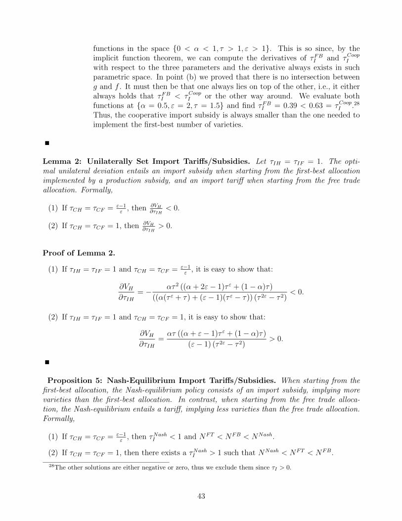
functions in the space {0 < α < 1, τ > 1, ε > 1}. This is so since, by theimplicit function theorem, we can compute the derivatives of τFBI and τCoopI

with respect to the three parameters and the derivative always exists in suchparametric space. In point (b) we proved that there is no intersection betweeng and f . It must then be that one always lies on top of the other, i.e., it eitheralways holds that τFBI < τCoopI or the other way around. We evaluate bothfunctions at {α = 0.5, ε = 2, τ = 1.5} and find τFBI = 0.39 < 0.63 = τCoopI .28

Thus, the cooperative import subsidy is always smaller than the one needed toimplement the first-best number of varieties.

Lemma 2: Unilaterally Set Import Tariffs/Subsidies. Let τIH = τIF = 1. The opti-mal unilateral deviation entails an import subsidy when starting from the first-best allocationimplemented by a production subsidy, and an import tariff when starting from the free tradeallocation. Formally,


, then ∂VH∂τIH

< 0.

(2) If τCH = τCF = 1, then ∂VH∂τIH

> 0.

Proof of Lemma 2.

(1) If τIH = τIF = 1 and τCH = τCF = ε−1ε

, it is easy to show that:

∂VH∂τIH

= − ατ 2 ((α + 2ε− 1)τ ε + (1− α)τ)

((α(τ ε + τ) + (ε− 1)(τ ε − τ)) (τ 2ε − τ 2)< 0.

(2) If τIH = τIF = 1 and τCH = τCF = 1, it is easy to show that:

∂VH∂τIH

=ατ ((α + ε− 1)τ ε + (1− α)τ)

(ε− 1) (τ 2ε − τ 2)> 0.

Proposition 5: Nash-Equilibrium Import Tariffs/Subsidies. When starting from thefirst-best allocation, the Nash-equilibrium policy consists of an import subsidy, implying morevarieties than the first-best allocation. In contrast, when starting from the free trade alloca-tion, the Nash-equilibrium entails a tariff, implying less varieties than the free trade allocation.Formally,


, then τNashI < 1 and NFT < NFB < NNash.

(2) If τCH = τCF = 1, then there exists a τNashI > 1 such that NNash < NFT < NFB.

28The other solutions are either negative or zero, thus we exclude them since τI > 0.

43

Proof of Proposition 5. In the case of tariffs, the non-cooperative policy maker maximizes:

maxτIH

VH(PH(τIH , τIF ), IH(τIH , τIF )) (69)

where PH(τIH , τIF ) is given by equation (36) once we substitute inNH(τIH , τIF ) andNF (τIH , τIF )as implicitly determined by equation (22). IH(τIH , τIF ) is equal to L+(τCH−1)NH(τIH , τIF )εf+

(τIH−1)τPFF (τIH , τIF )CHF (τIH , τIF ) where PFF (τIH , τIF ) = εε−1τCF (NF (τIH , τIF ))

11−ε , CHF (τIH , τIF )

= PHF (τIH , τIF )−εPH(τIH , τIF )εCH(τIH , τIF ), PHF (τIH , τIF ) = εε−1ττIHτCF (NF (τIH , τIF ))

11−ε

and finally CH(τIH , τIF ) is given by its equilibrium value in equation (37).


and τIH = τIF , the first-order condition of (69) with respect to τIHcan be written as:

ANashI (τI)

BNashI (τI)

= 0

where

ANashI (τI) ≡ α(ε− 2)ε2τ ε+3τ εI + (α− 1)ε(α + ε2 − 1

)τ ε+3τ ε+2

I

+ (α− 1)(ε2 + ε− 1

)(α + ε− 1)τ 2ε+2τ 2ε+2

I

− (α + ε− 1)(αε+ α + ε2 + ε− 1

)τ 3ε+1τ 3ε+1

I

+((1− 2α)ε3 + 2(α− 1)ε2 − (α− 1)αε+ (α− 1)2

)τ ε+3τ ε+1

I

+ ε(α(ε− 1)− 1)(α + ε− 1)τ 2ε+2τ 2εI+ ε(α + ε− 1)2τ 3ε+1τ 3εI − ε(α + ε− 1)((2α− 1)ε+ 2)τ 2ε+2τ 2ε+1

I

+ ε(α + ε− 1)2τ 4ετ 4εI − ε(α + ε− 1)2τ 4ετ 4ε+1I − (α− 1)2(ε− 1)ετ 4τ 3I

+ (α− 1)(ε− 1)τ 4τ 2I (α(2ε− 1)− ε+ 1) + (1− α)α(ε− 2)ετ 4τI

BNashI (τI) ≡ τI (τ ετ εI + ττI)

(τ 2ετ 2εI − τ 2

)((α + ε− 1)τ ετ εI + (α− 1)(ε− 1)ττI − α(ε− 2)τ)

((α + ε− 1)τ ετ εI + ττI(−αε+ α + ε− 1) + αετ)

The first part of Proposition 5 is proved by showing that if τCH = τCF = ε−1ε

: (i) thereis no solution of the Nash equilibrium of the non-cooperative policy game for τI > 1;(ii) if ε > 2, there exists a solution of the non-cooperative policy game for τI < 1; (iii)NNash > NFB > NFT .

(i) In order to show that no Nash equilibrium exists, we need to prove that there areno zeros of ANashI (τI) for τI > 1. This is so because: (a) ANashI is a second-order

polynomial in α; (b) if α = 0 or α = 1, ANashI (τI) < 0; (c)∂ANashI (τI)

∂τI|α=0 < 0.

(a) It is straightforward to see that ANashI is quadratic in α.

(b) If α = 0 and τI > 1

ANashI (τI) = −(ε− 1)(τ ε+3τ ε+1I ((ε+ 1)ετI − ε(ε− 1) + 1)

+ τ 2ε+2τ 2εI((ε2 + ε− 1

)τ 2I − (ε− 2)ετI + ε

)+ τ 3ε+1τ 3εI

((ε2 + ε− 1

)τI − (ε− 1)ε

)+ τ 4ετ 4εI (ε− 1)ε (τI − 1)

+ τ 4τ 2I (ε (τI − 1) + 1)) < 0

44

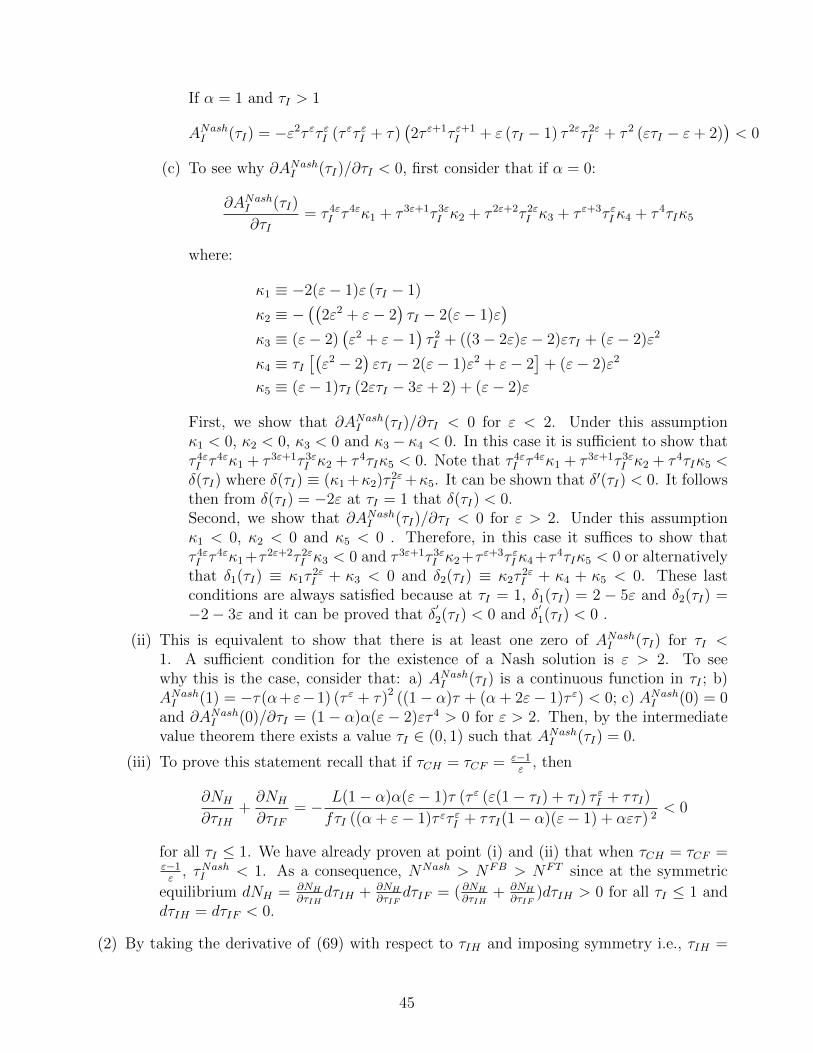
If α = 1 and τI > 1

ANashI (τI) = −ε2τ ετ εI (τ ετ εI + τ)(2τ ε+1τ ε+1

I + ε (τI − 1) τ 2ετ 2εI + τ 2 (ετI − ε+ 2))< 0

(c) To see why ∂ANashI (τI)/∂τI < 0, first consider that if α = 0:

∂ANashI (τI)

∂τI= τ 4εI τ

4εκ1 + τ 3ε+1τ 3εI κ2 + τ 2ε+2τ 2εI κ3 + τ ε+3τ εI κ4 + τ 4τIκ5

where:

κ1 ≡ −2(ε− 1)ε (τI − 1)

κ2 ≡ −((

2ε2 + ε− 2)τI − 2(ε− 1)ε

)κ3 ≡ (ε− 2)

(ε2 + ε− 1

)τ 2I + ((3− 2ε)ε− 2)ετI + (ε− 2)ε2

κ4 ≡ τI[(ε2 − 2

)ετI − 2(ε− 1)ε2 + ε− 2

]+ (ε− 2)ε2

κ5 ≡ (ε− 1)τI (2ετI − 3ε+ 2) + (ε− 2)ε

First, we show that ∂ANashI (τI)/∂τI < 0 for ε < 2. Under this assumptionκ1 < 0, κ2 < 0, κ3 < 0 and κ3 − κ4 < 0. In this case it is sufficient to show thatτ 4εI τ

4εκ1 + τ 3ε+1τ 3εI κ2 + τ 4τIκ5 < 0. Note that τ 4εI τ4εκ1 + τ 3ε+1τ 3εI κ2 + τ 4τIκ5 <

δ(τI) where δ(τI) ≡ (κ1 +κ2)τ2εI +κ5. It can be shown that δ′(τI) < 0. It follows

then from δ(τI) = −2ε at τI = 1 that δ(τI) < 0.Second, we show that ∂ANashI (τI)/∂τI < 0 for ε > 2. Under this assumptionκ1 < 0, κ2 < 0 and κ5 < 0 . Therefore, in this case it suffices to show thatτ 4εI τ

4εκ1+τ 2ε+2τ 2εI κ3 < 0 and τ 3ε+1τ 3εI κ2+τ ε+3τ εI κ4+τ 4τIκ5 < 0 or alternativelythat δ1(τI) ≡ κ1τ

2εI + κ3 < 0 and δ2(τI) ≡ κ2τ

2εI + κ4 + κ5 < 0. These last

conditions are always satisfied because at τI = 1, δ1(τI) = 2 − 5ε and δ2(τI) =−2− 3ε and it can be proved that δ

′2(τI) < 0 and δ

′1(τI) < 0 .

(ii) This is equivalent to show that there is at least one zero of ANashI (τI) for τI <1. A sufficient condition for the existence of a Nash solution is ε > 2. To seewhy this is the case, consider that: a) ANashI (τI) is a continuous function in τI ; b)ANashI (1) = −τ(α+ε−1) (τ ε + τ)2 ((1− α)τ + (α + 2ε− 1)τ ε) < 0; c) ANashI (0) = 0and ∂ANashI (0)/∂τI = (1 − α)α(ε − 2)ετ 4 > 0 for ε > 2. Then, by the intermediatevalue theorem there exists a value τI ∈ (0, 1) such that ANashI (τI) = 0.

(iii) To prove this statement recall that if τCH = τCF = ε−1ε

, then

∂NH

∂τIH+∂NH

∂τIF= − L(1− α)α(ε− 1)τ (τ ε (ε(1− τI) + τI) τ

εI + ττI)

fτI ((α + ε− 1)τ ετ εI + ττI(1− α)(ε− 1) + αετ) 2< 0

for all τI ≤ 1. We have already proven at point (i) and (ii) that when τCH = τCF =ε−1ε

, τNashI < 1. As a consequence, NNash > NFB > NFT since at the symmetric

equilibrium dNH = ∂NH∂τIH


dτIF = ( ∂NH∂τIH

+ ∂NH∂τIF

)dτIH > 0 for all τI ≤ 1 anddτIH = dτIF < 0.

(2) By taking the derivative of (69) with respect to τIH and imposing symmetry i.e., τIH =

45

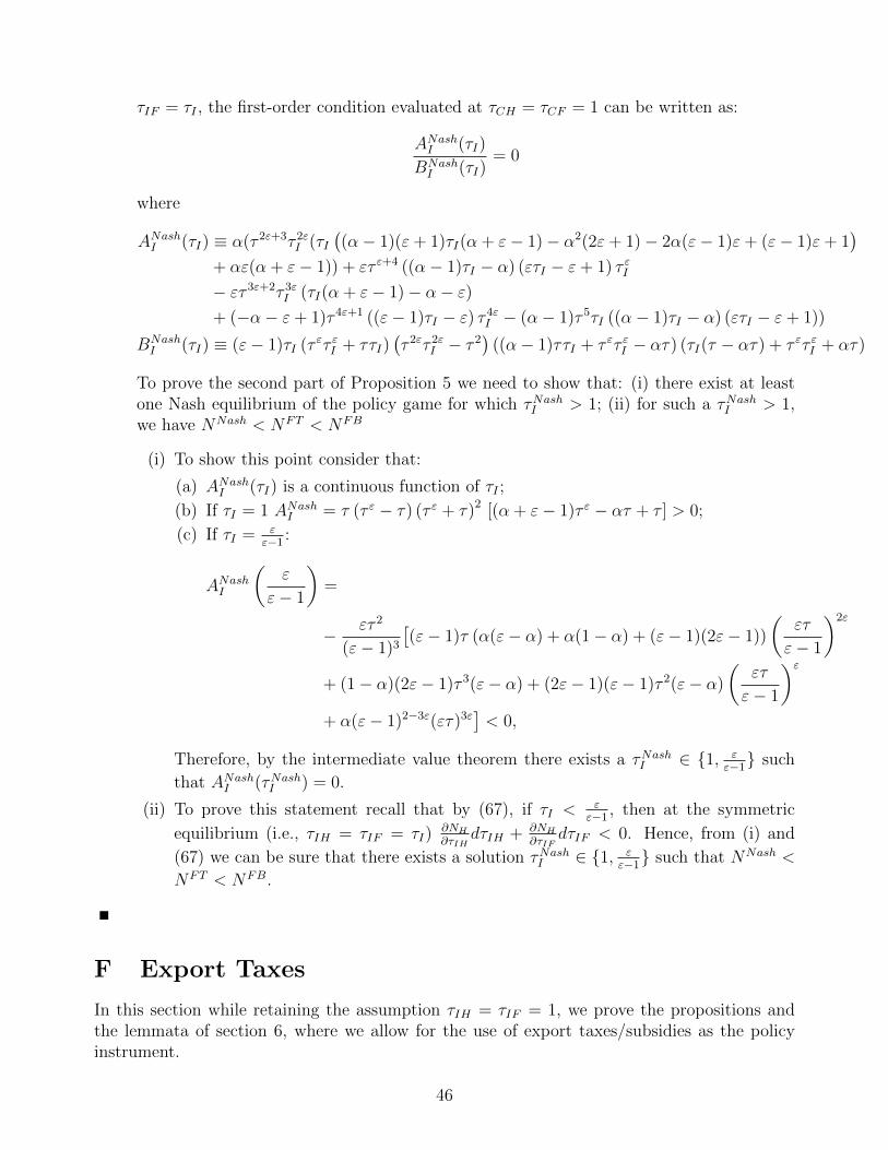
τIF = τI , the first-order condition evaluated at τCH = τCF = 1 can be written as:

ANashI (τI)

BNashI (τI)

= 0

where

ANashI (τI) ≡ α(τ 2ε+3τ 2εI (τI((α− 1)(ε+ 1)τI(α + ε− 1)− α2(2ε+ 1)− 2α(ε− 1)ε+ (ε− 1)ε+ 1

)+ αε(α + ε− 1)) + ετ ε+4 ((α− 1)τI − α) (ετI − ε+ 1) τ εI− ετ 3ε+2τ 3εI (τI(α + ε− 1)− α− ε)+ (−α− ε+ 1)τ 4ε+1 ((ε− 1)τI − ε) τ 4εI − (α− 1)τ 5τI ((α− 1)τI − α) (ετI − ε+ 1))

BNashI (τI) ≡ (ε− 1)τI (τ ετ εI + ττI)

(τ 2ετ 2εI − τ 2

)((α− 1)ττI + τ ετ εI − ατ) (τI(τ − ατ) + τ ετ εI + ατ)

To prove the second part of Proposition 5 we need to show that: (i) there exist at leastone Nash equilibrium of the policy game for which τNashI > 1; (ii) for such a τNashI > 1,we have NNash < NFT < NFB

(i) To show this point consider that:

(a) ANashI (τI) is a continuous function of τI ;

(b) If τI = 1 ANashI = τ (τ ε − τ) (τ ε + τ)2 [(α + ε− 1)τ ε − ατ + τ ] > 0;

(c) If τI = εε−1 :

ANashI

(ε

ε− 1

)=

− ετ 2

(ε− 1)3[(ε− 1)τ (α(ε− α) + α(1− α) + (ε− 1)(2ε− 1))

(ετ

ε− 1

)2ε

+ (1− α)(2ε− 1)τ 3(ε− α) + (2ε− 1)(ε− 1)τ 2(ε− α)

(ετ

ε− 1

)ε+ α(ε− 1)2−3ε(ετ)3ε

]< 0,

Therefore, by the intermediate value theorem there exists a τNashI ∈ {1, εε−1} such

that ANashI (τNashI ) = 0.

(ii) To prove this statement recall that by (67), if τI <εε−1 , then at the symmetric

equilibrium (i.e., τIH = τIF = τI)∂NH∂τIH


dτIF < 0. Hence, from (i) and

(67) we can be sure that there exists a solution τNashI ∈ {1, εε−1} such that NNash <

NFT < NFB.

F Export Taxes

In this section while retaining the assumption τIH = τIF = 1, we prove the propositions andthe lemmata of section 6, where we allow for the use of export taxes/subsidies as the policyinstrument.

46

Lemma A3: Policy Incentives for Export Subsidies/Taxes If τCH = τCF = 1, thenwhen there is a symmetric increase in the export subsidies in Home and in Foreign, productionefficiency effects are positive. At the same time, if τXH = τXF = τCH = τCF = 1, when thereis a unilateral increase in export subsidies at Home, the production efficiency effect is positivein the domestic economy and negative in the foreign one, while domestic terms-of-trade effectsare negative. If τCH = τCF = ε−1

εand τXH = τXF = 1, a unilateral increase in the export tax

at Home generates positive terms-of-trade effects. Formally,

(1) Let τCH = τCF = 1 and τXH = τXF ≤ 1. If dτXH = dτXF < 0, then( εε−1−1)(y+f)dNH

IH=


IF> 0.

(2) Let τXH = τXF = τCH = τCF = 1. If dτXH < 0, then( εε−1−1)(y+f)dNH

IH> 0,


IF<

0 and d(τXHPHH)τCFH−d(τXFPFF )τCHFIH

< 0.

(3) Let τXH = τXF = 1 and τCH = τCF = ε−1ε

. If dτXH > 0, then d(τXHPHH)τCFH−d(τXFPFF )τCHFIH

>0.

Proof of Lemma A3.

(1) Let τCH = τCF = 1. By imposing symmetry, we obtain:

dNH = dNF =∂NH

∂τXHdτXH +

∂NH

∂τXFdτXF =

(∂NH

∂τXH+∂NF

∂τXH

)dτXH

When 0 < τXH = τXF ≤ 1 the following derivative is negative:

∂NH

∂τXH+∂NF

∂τXH= −L(1− α)ατ(τXτ + (τXτ)ε(τX + ε(1− τX)))

fτXε(ατ + (τXτ)ε + τXτ(1− α))2< 0

which implies that dNH = dNF > 0 ⇐⇒ dτHX = dτXF < 0 i.e., symmetric productionsubsidies generate positive production efficiency effects for both Home and Foreign.

(2) Let τXH = τXF = τCH = τCF = 1. The change in the number of Home and Foreignvarieties when τXH moves unilaterally is given by:

dNH =∂NH

∂τXHdτXH = −Lατ(τ 2 + (ε− α)τ 2ε + (ε− 1 + α)τ 1+ε

fε(τ − τ ε)2(τ + τ ε)dτXH

dNF =∂NF

∂τXHdτXH =

Lατ(ατ 2 + (ε− 1)τ 2ε + (ε− 1 + α)τ 1+ε

fε(τ − τ ε)2(τ + τ ε)dτXH

Therefore, dNH > 0 and dNF < 0 ⇐⇒ dτXH < 0. Thus, unilateral increase in the exportsubsidy generates production efficiency effects that are positive for Home and negativefor Foreign.

47

Once we impose symmetry and we assume that τXH = τXF = 1, terms-of-trade effects in(35) can be written as:(

εε−1N

− 1ε−1

H dτXH − τCHε−1

εε−1N

− εε−1

H dNH + τCFε−1

εε−1N

− εε−1

F dNF

)τCHF

IH(70)

We just showed that dτXH < 0 implies dNH > 0 and dNF < 0, i.e., unilaterally setexport subsidies generate negative consumption based terms-of-trade effects both directly,through their impact on the price of exported varieties, and indirectly, through theirimpact on the number of Home and Foreign varieties.

(3) It remains to show is that when τCH = τCF = ε−1ε

and dτXH > 0 then dNH < 0 anddNF > 0. This follows from the fact that:

∂NH

∂τXH= −Lα(ε− 1)τ (τ 2 (α2 + ε− 1) + (α(2ε− 1) + (ε− 1)2) τ ε+1 + (ε− α)(α + ε− 1)τ 2ε)

f(α + ε− 1)2 (τ 2ε − τ 2) (α(τ ε + τ) + (ε− 1)(τ ε − τ))< 0

∂NF

∂τXH=Lα(ε− 1)τ ((α + ε2 − 1) τ ε+1 + (ε− 1)(α + ε− 1)τ 2ε + αετ 2)

f(α + ε− 1)2 (τ 2ε − τ 2) (α(τ ε + τ) + (ε− 1)(τ ε − τ))> 0

Proposition 6: Cooperative Export Subsidy. If τCH = τCF = ε−1ε

, the cooperative policymaker refrains from using taxes on exports and the number of varieties equals the first-bestlevel. If τCH = τCF = 1, the cooperative policy maker finds it optimal to subsidize exports.The number of varieties is larger than in the free trade allocation, but remains lower than thefirst-best level. Formally,


, then τCoopX = 1 and NCoop = NFB.

(2) If τCH = τCF = 1, then τCoopX < 1 and NFT < NCoop < NFB.

Proof of Proposition 6.


, the cooperative policy maker solves:

maxτXH ,τXF

VH(PH(τXH , τXF ), IH(τXH , τXF )) + VF (PF (τXH , τXF ), IF (τXH , τXF )) (71)

Here, PH(τXH , τXF ) is given by equation (36), which is implied by the equilibrium ex-pressions for NH(τXH , τXF ) and NF (τXH , τXF ), equation (41). IH(τXH , τXF ), is givenby LH + (τXH − 1)τPHH(τXH , τXF )CFH(τXH , τXF ) + (τCH − 1)NH(τXH , τXF )εf where

PHH(τXH , τXF ) = εε−1τCHNH(τXH , τXF )

11−ε , CFH(τXH , τXF ) = PFH(τXH , τXF )−εPF (τXH , τXF )ε

CF (τXH , τXF ) and PFH(τXH , τXF ) = εε−1ττXHτCHNH(τXH , τXF )

11−ε . Finally, CH(τXH , τXF )

is given by its equilibrium value in equation (37). Symmetric conditions apply to foreignvariables.

48

Taking derivatives with respect to τXH and τXF and imposing symmetry, the first-ordercondition can be written as:

αετ(τX − 1)[(α + ε− 1)τ 2ετ 2εX + (1− α)τ 2τX + ετ ε+1τ εX ]

τX(τ ετ εX + τ)(τ ετ εX + ττX)[−(α + ε− 1)τ ετ εX + (α− 1)(ε− 1)ττX − αετ ]= 0

It is straightforward to see that τX = 1 is the unique solution to this equation. We havealready shown in Proposition 2 that τCH = τCF = ε−1

ε, τXH = τXF = 1 implements the

first-best allocation. Thus, NCoop = NFB.

(2) If τCH = τCF = 1, the cooperative policy maker solves the same problem as in (1) butincome is now given by IH(τXH , τXF ) = L+(τXH−1)τPHHCFH and similarly for Foreign.Taking derivatives with respect to τXH and τXF and imposing symmetry, the first-ordercondition can now be written as

ACoopX (τX)

BCoopX (τX)

= 0,

where

ACoopX (τX) ≡ ατ [τ ε+1τ εX [τX(2α− ε2 + ε− 2) + (ε− 1)ε]

+ τ 2ετ 2εX [ε(α + ε− 2)− (ε− 1)τX(α + ε− 1)] + (α− 1)τ 2τX(ετX − ε+ 1)]

BCoopX (τX) ≡ (ε− 1)τX(τ ετ εX + τ)(τ ετ εX + ττX)(τX(τ − ατ) + τ ετ εX + ατ)

Note that ACoopX (τX) = ACoopI (τI) and BCoopX (τX) = BCoop

I (τI) with the only difference thatthey are functions of τX instead of τI . Thus, the proof is the same as the one for thecooperative import subsidy (Proposition 4).

Lemma 3: Unilaterally Set Export Taxes/Subsidies. Let τXH = τXF = 1. The optimalunilateral deviation entails an export tax when starting from the first-best allocation implementedby a production subsidy, and an export subsidy when starting from the free trade allocation.Formally,


, then ∂VH∂τXH

> 0.

(2) If τCH = τCF = 1, then ∂VH∂τXH

< 0.

Proof of Lemma 3:


, then:

∂VH∂τX

=ατ ((1− α)τ ε+1 + (α + ε− 1)τ 2ε + ετ 2)

(τ 2ε − τ 2) (α(τ ε + τ) + (ε− 1)(τ ε − τ))> 0

49

(2) If τCH = τCF = 1, then:

∂VH∂τXH

= −ατ (τ(α + ε− 1) + (1− α)τ ε)

(ε− 1) (τ 2ε − τ 2)< 0

Proposition 7: Nash-Equilibrium Export Taxes/Subsidies. When starting from thefirst-best allocation, the Nash-equilibrium policy consists of an export tax, implying less varietiesthan the first-best allocation. In contrast, when starting from the free trade allocation, the Nash-equilibrium entails an export subsidy, implying more varieties than the free trade allocation.Formally,


, then τNashX > 1 and NNash < NFB.

(2) If τCH = τCF = 1, then τNashX < 1 and NFT < NNash < NFB.

Proof of Proposition 7.


, the Nash policy maker solves:

maxτXH

VH(PH(τXH , τXF ), IH(τXH , τXF )) (72)

Here, PH(τXH , τXF ) is given by equation (36), which is implied by the equilibrium expres-sions for NH(τXH , τXF ) and NF (τXH , τXH), equation (41). Moreover, I(τXH , τXF ) = L+(τXH−1)τPHH(τXH , τXF )CFH(τXH , τXF )+(τCH−1)NH(τXH , τXF )εf , where PHH(τXH , τXF )

= εε−1τCHNH(τXH , τXF )

11−ε , CFH = PFH(τXH , τXF )−εPF (τXH , τXF )εCF (τXH , τXF ), PFH(τXH , τXF )

= εε−1ττXHτCHNH(τXH , τXF )

11−ε and finally CF (τXH , τXF ) is given by its equilibrium value

in equation (37).

Taking derivatives with respect to τXH and τXF and then imposing symmetry i.e., τXH =τXF = τX , the first-order conditions at the symmetric Nash equilibrium can be written as

ANashX (τX)

BNashX (τX)

= 0 (73)

where

ANashX (τX) ≡ ατ{−τ ε+3τ ε+1X [τX((α2 − 1)(ε− 1)ετX + (−2α2 + α− 2)ε2 + (α− 1)2 + ε3)

+ ε((α− 1)αε+ (α− 1)α− ε2 + ε)]

+ τ 2ε+2τ 2εX [τX(ετX(α2 + α(ε− 1)2 − (ε− 2)(ε− 1))

− α2(ε+ 1) + 2α(−ε3 + ε2 + 1) + (ε− 1)(ε2 + 1)) + αε3]

+ τ 3ε+1τ 3εX (α + ε− 1)[(ε− 1)τX (τX(α(ε− 1) + 1)− (2α + 1)ε) + (α + 1)ε2]

− τ 4εX τ 4ε(α + ε− 1)2[(ε− 1)τX − ε] + τ 4τ 2Xε(α + ε− 1)}

50

BNashX (τX) ≡ τX(τ ετ εX + ττX)(τ 2ετ 2εX − τ 2)[(α + ε− 1)τ ετ εX − (α + 1)(ε− 1)ττX + αετ ]

[(α + ε− 1)τ ετ εX + ττX(−αε+ α + ε− 1) + αετ ]

(i) We first show that no solution with τX < 1 exists. Focusing on the numerator of thefirst-order condition, this is so since all terms of ANashX (τX) are positive for τX < 1.

(ii) Next, we show that there exists at least one solution with τX > 1.

(a) For τX = 1, ANashX (1) = (ε+α−1) (τ ε + τ)2 [(1−α)τ ετ+ετ 2+τ 2ε(ε−1+α)] > 0;

(b) limτX→∞ANashX (τX) = −∞;

(c) Thus, by continuity ofANashX (τX), there exists a τNashX > 1 such thatANashX (τNashX ) =0.

(iii) It remains to show that if τNashX > 1, then NNash < NFB. When τCH = τCF = ε−1ε

and after imposing symmetry i.e., τXH = τXF = τX and dτXH = dτXF :

dNH =∂NH

∂τXHdτXH +

∂NH

∂τXFdτXF =

(∂NH

∂τXH+∂NH

∂τXF

)dτXH

=L(1− α)α(ε− 1)τ [τ ετ εX ((ε− 1)τX − ε)− ττX ]

fτX [(α + ε− 1)τ ετ εX + ττX(1− α)(ε− 1) + αετ ]2dτXH

Note that dτXH > 0 ⇒ dNH ≥ 0 ⇐⇒ τ ετ εX [(ε− 1)τX − ε] − ττX ≥ 0. Let usdefine the following two continuous and monotonic functions f(τX) ≡ (ε− 1)τ ετ ε+1

X

and g(τX) ≡ ετ ετ εX + ττX with f ′(τX) > 0, f ′′(τX) > 0, g′(τX) > 0 and g′′(τX) > 0.Note that f(1)− g(1) < 0 implying that dNH < 0 when τX = 1. By continuity andmonotonicity of the two functions, only two cases are possible. They either nevercross, in which case dNH < 0∀τX ∈ [1,∞) and consequently NNash < NFB. Or,they cross only once. That implies that ∃τX > 1 such that f(τX) ≥ g(τX), ∀τX ≥ τXimplying dNH > 0 ⇐⇒ τX ∈ (τX ,∞). However note that:

limτX−>∞

NH = limτX−>∞

Lα (τ ετ εX + τ)

f ((α + ε− 1)τ ετ εX + ττX(α(−ε) + α + ε− 1) + αετ)= NFB

implying that also in this case NNash < NFBX .

(2) If τCH = τCF = 1, the Nash policy maker solves the same problem as in (1) but incomeis now given by IH(τXH , τXF ) = L + (τXH − 1)τPHH(τXH , τXF )CFH(τXH , τXF ). Takingderivatives with respect to τXH and τXF and then imposing symmetry i.e., τXH = τXF =τX , the first-order conditions at the symmetric Nash equilibrium can be written as:

ANashX (τX)

BNashX (τX)

= 0 (74)

51

with

ANashX (τX) ≡ α{τ ε+4τ ε+1X [τX(τX(ε− α2ε) + 2α2ε+ (α− 1)α− ε2 + ε)− α2(ε+ 1) + α+ (ε− 1)ε]

+ τ2ε+3τ2εX [τX(τX((α− 1)ε2 − α+ ε+ 1) + α(−2ε2 + ε− 1) + (ε− 1)2) + α(ε− 1)ε]

+ τ3ε+2τ3εX [τX(α(ε− 1)τX(α+ ε− 1)− (2α+ 1)ε2 − 2(α− 2)αε+ (α− 1)α)

+ ε(α(α+ ε− 2) + ε− 1)]

+ τ4ε+1τ4εX (ε(α+ ε− 2)− (ε− 1)τX(α+ ε− 1)) + τ5τ2X(α+ ε− 1)}BNashX (τX) ≡ (ε− 1)τX(τ ετ εX + ττX)(τ2ετ2εX − τ2)(−(α+ 1)ττX + τ ετ εX + ατ)

(τX(τ − ατ) + τ ετ εX + ατ)

(i) In order to show that there exists a solution with τX < 1, we first show that whenτX = 1, ANashX (1) is negative. This is so given that ANashX (1) = τ(τ ε−τ)(τ ε +τ)2[(α−1)τ ε + τ(−α− ε+ 1)] < 0.

(ii) Next, we show that for ε > 2 there exists a τX ∈ {0, 1} with ANashX (τX) > 0.By continuity of ANashX (τX) this is enough to guarantee the existence of a solution.Consider τX = ε−2

ε. Then,

ANashX ( ε−2ε

) = τε2

[(ε− 2)2τ 4(α+ ε− 1) + (ε− 2)4εε1−4ε(2 + 2ε2− 5ε+ 3αε− 2α)τ 4ε +

(ε−2)1+εε−ε(4+2α−6α2+3(ε−2)ε)τ 3+ε+(ε−2ε

)2ε(α(6ε−4)+(ε−2)(ε2−2))τ 2+2ε+

τ (α2(6ε− 4) + 2α(ε− 2)(2ε− 1) + ε3)(

(ε−2)τε

)3ε] > 0 since each of the coefficients

is positive for ε > 2. This proves that a solution with τX < 1 exists.

(iii) Finally, we show that NNash < NFB.

(a) Let τNashX = f(α, ε, τ) and τFBX = g(α, ε, τ) be, respectively, the Nash equi-librium export subsidy and the export subsidy that implements the first-bestnumber of varieties . First we show that there is no intersection between the setof τNashX and the set of τFBX in the interval [0, 1]. If τX = τNashX , ANashX (τNashX ) = 0.

At the same time τFBX is such N =Lα(τ+(ττFBX )ε)

fε(ατ+τ(1−α)τFBX +(ττFBX )ε)= Lα

f(ε+α−1) = NFB.

This last condition can be rewritten as (ττX)ε = −εττX + τ(ε − 1). Note thatwhen combined, this two conditions are a system of two equations in τX . Wenow investigate if there exists a τX such that both conditions are satisfied si-multaneously. Once we substitute the above condition into ANashX we obtain afifth-order polynomial in τX which can be factorized into two polynomials. Thefirst polynomial is −ετ 5 (τX − 1) 2(α+ ε− 1), with solutions τX = {1, 1}. Noneof these solutions solves (ττX)ε = −εττX + τ(ε− 1). The second polynomial iscubic and we call it AX

Nashmod . It can be shown that there exist at most one real

solution of AXNashmod . However, evaluating AX

Nashmod at τX = 1 and τX = 0 we find

that both AXNashmod (1) < 0 and AX

Nashmod (0) < 0. Thus, by continuity of AX

Nashmod ,

either there exists no real solution or there are at least two zeros of AXNashmod = 0

that are real. Since there exists at most one real solution of AXNashmod = 0 in [0, 1],

we can conclude that there is no intersection between the set of τNashX and theset of τFBX in the interval [0, 1].

(b) The second step is to show that τFBX < τNashX in the interval [0, 1]. To thisend, recall that f and g are two continuous functions in the space {0 < α <1, τ > 1, ε > 1}, given that the derivatives of τFBX and τNashX with respect to the

52

three parameters always exists in the permitted parameter space. In point (a)we proved that there is no intersection between g and f . As a consequence, weeither have τFBX < τNashX or the other way around. We evaluate both functionsat {α = 0.5, ε = 2, τ = 1.5} and find τFBX = 0.39 < 0.82 = τNashX . Thus, the non-cooperative export subsidy is always smaller than the one needed to implementthe first-best number of varieties.

(c) Finally, from Lemma A3 (1) we know that 0 < τXH = τXF ≤ 1 ⇒ ∂NH∂τXH

+∂NF∂τXH

< 0 which implies that dNH = dNF > 0 ⇐⇒ dτHX = dτXF < 0 i.e,by symmetrically increasing the export subsidy in both countries policy makersincrease the number of varieties. It then follows that τFBX < τNashX ⇒ NNash <NFB.

G Simultaneous Policy Choice

Proposition 8: Cooperative Policy Instruments. The cooperative policy maker sets thefirst-best level of production subsidies and chooses the trade taxes such that τCoopI · τCoopX = 1.The number of varieties equals the first-best level.


, τCoopI · τCoopX = 1 and NCoop = NFB.

Proof of Proposition 8. We have already proven in Propositions 2, 4 and 6 that the first-best allocation can be implemented by eliminating the monopolistic distortion and by refrainingfrom using import or export taxes (i.e., by setting τCoopC = ε−1

εand τCoopI = τCoopX = 1). What

remains to show is that the first-best allocation can be implement even when τCoopC = ε−1ε

and

τCoopI τCoopX = 1. To see why this is the case, notice that if τCoopC = ε−1ε

and τCoopI τCoopX = 1 NH =

NF = NFB, i.e., this policy implements the first-best allocation. Intuitively, if τCoopC = ε−1ε

any

policy such that τCoopI τCoopX = 1 allows to reach the social optimum since the effects of importtariffs/subsidies are exactly offset by those of export subsidies/taxes.

Proposition 9: Nash-Equilibrium Policy Instruments. The Nash-equilibrium policyconsists of the first-best level of production subsidies, and inefficient import subsidies and exporttaxes. Formally,

(1) τNashC = τCoopC = ε−1ε

, τNashI < 1, τNashX > 1.

Proof of Proposition 9. In order to prove Proposition 9 we follow Dixit (1985) and we usethe primal approach to optimal policy instead of the indirect utility function i.e., we directlymaximize utility subject to the equilibrium conditions. The non-cooperative policy makermaximizes domestic utility subject to the good market clearing conditions, the trade balance

53

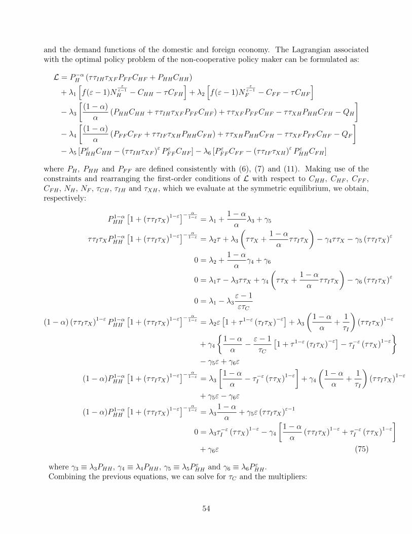
and the demand functions of the domestic and foreign economy. The Lagrangian associatedwith the optimal policy problem of the non-cooperative policy maker can be formulated as:

L = P−αH (ττIHτXFPFFCHF + PHHCHH)

+ λ1

[f(ε− 1)N

εε−1

H − CHH − τCFH]

+ λ2

[f(ε− 1)N

εε−1

F − CFF − τCHF]

− λ3[

(1− α)

α(PHHCHH + ττIHτXFPFFCHF ) + ττXFPFFCHF − ττXHPHHCFH −QH

]− λ4

[(1− α)

α(PFFCFF + ττIF τXHPHHCFH) + ττXHPHHCFH − ττXFPFFCHF −QF

]− λ5 [P ε

HHCHH − (ττIHτXF )ε P εFFCHF ]− λ6 [P ε

FFCFF − (ττIF τXH)ε P εHHCFH ]

where PH , PHH and PFF are defined consistently with (6), (7) and (11). Making use of theconstraints and rearranging the first-order conditions of L with respect to CHH , CHF , CFF ,CFH , NH , NF , τCH , τIH and τXH , which we evaluate at the symmetric equilibrium, we obtain,respectively:

P 1−αHH

[1 + (ττIτX)1−ε

]− α1−ε = λ1 +

1− αα

λ3 + γ5

ττIτXP1−αHH


]− α1−ε = λ2τ + λ3

(ττX +

1− αα

ττIτX

)− γ4ττX − γ5 (ττIτX)ε

0 = λ2 +1− αα

γ4 + γ6

0 = λ1τ − λ3ττX + γ4

(ττX +

1− αα

ττIτX

)− γ6 (ττIτX)ε

0 = λ1 − λ3ε− 1

ετC

(1− α) (ττIτX)1−ε P 1−αHH


]− α1−ε = λ2ε

[1 + τ 1−ε (τIτX)−ε

]+ λ3

(1− αα

+1

τI

)(ττIτX)1−ε

+ γ4

{1− αα− ε− 1

τC

[1 + τ 1−ε (τIτX)−ε

]− τ−εI (ττX)1−ε

}− γ5ε+ γ6ε

(1− α)P 1−αHH


]− α1−ε = λ3

[1− αα− τ−εI (ττX)1−ε

]+ γ4

(1− αα

+1

τI

)(ττIτX)1−ε

+ γ5ε− γ6ε

(1− α)P 1−αHH


]− α1−ε = λ3

1− αα

+ γ5ε (ττIτX)ε−1

0 = λ3τ−εI (ττX)1−ε − γ4

[1− αα

(ττIτX)1−ε + τ−εI (ττX)1−ε]

+ γ6ε (75)

where γ3 ≡ λ3PHH , γ4 ≡ λ4PHH , γ5 ≡ λ5PεHH and γ6 ≡ λ6P

εHH .

Combining the previous equations, we can solve for τC and the multipliers:

54

τC =ε− 1

ε

λ1 = γ3 = P 1−αHH α


]− α1−ε

γ4 =P 1−αHH α

2(1− α)(ε(τX − 1)− τX) [1 + (ττIτX)1−ε]− α

1−ε

(ε− 1)(α + (1− α)τI)τX

γ5 = 0

γ6 = −P1−αHH ατ

1−ε(τIτX)−ε [1 + (ττIτX)1−ε]− α

1−ε

ε− 1

λ2 = −γ6 −γ4α

(76)

The first condition in (76) already states that the Nash equilibrium production subsidy com-pletely offsets the monopolistic distortion. What remains to show is that τNashI < 1 andτNashX > 1. Substituting the expressions for the multipliers and the solution for τC in the first-order conditions and simplifying, we are left with two equations, the derivative with respect toCHF and the one with respect to NF . The derivative with respect to CHF is given by:

A1(τI , τX) + A2(τI , τX) + A3(τI , τX) = 0 (77)

where:

A1(τI , τX) ≡ −(ε− 1)(1− τI)τ 2X(α + (1− α)τI)

A2(τI , τX) ≡ −(ε− (ε− 1)τX)(ατX + 1− α)

A3(τI , τX) ≡ −(α + (1− α)τI)(ττX)1−ετ−εI

Note that:

(i) A3(τI , τX) < 0 always;

(ii) A1(τI , τX) < 0 ⇐⇒ τI < 1;

(iii) A2(τI , τX) < 0 ⇐⇒ τX < εε−1 .

Thus, a necessary condition for τI and τX to solve equation (77) is that if τX < εε−1 then

τI > 1. By combining (77) with the first-order condition with respect to NF we obtain a secondcondition:

B1(τI , τX) +B2(τI , τX) +B3(τI , τX) = 0 (78)

where

B1(τI , τX) ≡ −τ 2X(ε− 1)(α + (1− α)τI)(1− ε(1− τI))B2(τI , τX) ≡ (−ε+ τX(ε− 1))(ε− (1− α))τ ε−1(τIτX)ε

B2(τI , τX) ≡ −α(−ε+ τX(ε− 1))2

Note that:

55

(i) B3(τI , τX) < 0 always;

(ii) B1(τI , τX) < 0 ⇐⇒ τI >ε−1ε

;

(iii) B2(τI , τX) < 0 ⇐⇒ τX < εε−1 .

Thus, a necessary condition for τI and τX to solve equation (78) is that if τX < εε−1 then

τI <ε−1ε

. Note that this condition contradicts the one needed for (77). Therefore, the onlypossible solution is τNashX > ε

ε−1 i.e., this proves that τNashX > 1.

We now have to show that τNashI < 1. We will prove this by contradiction. First, we showthat a necessary condition for τNashI > 1 is that τNashI · τNashX < 1. Second, we show that ifτNashI > 1 it must be that τNashX < 1, which contradicts the fact that τNashX > 1. In order toshow the first point, it is useful to rewrite equation (77) as follows:

−(ε−1)(1−τI)τX(ατX +(1−α)τIX)+((ε−1)τX−ε)(ατX +1−α)− (ατX +(1−α)τIX)(τ1−ετ−εIX) = 0

where τIX ≡ τIτX . If we solve the previous equation for τI we obtain:

τNashI =C1(τX , τIX)

C2(τX , τIX)(79)

where:

C1(τX , τIX) ≡ (τIXτ)−ε(τIXτ(1− α) + (τIXτ)εε(1− α− τX + 2ατX)

+ ατXτ + (τIXτ)ετX(1− α) + τ 1+εIX τ ετX(ε− 1)(1− α))

C2(τX , τIX) ≡ (ε− 1)τX(τIX(1− α) + ατX)

Now suppose that τI > 0 and C2(τX , τIX) > 0, it has to be the case that C1(τX , τIX) > 0 too.Moreover, for τNashI to be greater than 1, C1(τX , τIX)− C2(τX , τIX) should be greater than 0:

C3(τI , τX) ≡ C1(τX , τIX)− C2(τX , τIX) =

(τIXτ)−ε(τIXτ(1− α) + αττX + (τIXτ)ε((1− α)ε+ (1− α+ 2τIX(1− α)(ε− 1)− ε+ 2αε)τX + α(ε− 1)τ2X)

Note that:

(i) C3(τI , τX) is linear in α;

(ii) α = 0 and τIX > 1 implies C3 = −(τIXτ)−ε(τIXτ+(τIXτ)ε(ε+(ε−1)(τIX−1)+τIXτX(ε−1))) < 0;

(iii) α = 1 and τIX > 1 implies C3 = −(τIXτ)−ε(ττX + (ττIX)ε(ετX + (ε− 1)τ 2X)) < 0;

(iv) By continuity, ∀α ∈ (0, 1) τIX > 1⇒ C3 < 0⇒ τNashI < 1;

(v) Thus, a necessary condition for τNashI > 1 is τIX < 1 .

However, we have already proven that τNashX > 1 thus, it cannot be that τNashI > 1 andτNashIX ≡ τNashI τNashX < 1. Therefore, it has to be that τNashI < 1.

56

trade policy: home market e ect versus terms-of-trade...

Documents