trade in services and trade in goods: differences and ... · pdf filetrade in services and...

Trade in Services and Trade in Goods: Differences and Complementarities

Carolina Lennon1

Preliminary Version . Please do not cite or quote without permission. Comments are very welcome. First Version: August 31, 2006 Abstract

Despite the increasing importance of services in national economies (accounting for about 50-70 % of internal product), in global economy (accounting for the 20 % of global trade) and in public opinion (i.e. US Concern about Mexican workers due to migration laws or the case of the “polish plumbers” in France at the time of European Constitution referendum) there is no economic consensus about the way in what services should be considered in trade liberalization analyses. Some economists argue that trade in services is not really much different from trade in goods, while others claim for the existence of specificities. The double purpose of this paper is; first, to empirically determine to what extent trade in services differs from trade in goods and, second, to explore the potential complementarity between bilateral trade in goods and bilateral trade in services. For our first goal we regress a set of equations derived from the gravitational model and for the second we instrument bilateral trade for both services and goods in order to analyse potential causalities of each type of flow in the other. Main results show that “bilateral trust and contract enforcement environment”, “Networks”, “labor markets” and “technology and technology of communication” have more impact on service trade than on trade in goods; finally, after instrumenting for endogeneity, we found that bilateral trade in goods explains bilateral trade in services: the resulting estimated elasticity is close to 1. Reciprocally, bilateral trade in services affects positively bilateral trade in goods: a 10% increase in trade in services raises traded goods by 4.58%.

1 University of Paris 1 (Panthéon-Sorbonne, CES) and Paris-Jourdan Sciences Economiques (PSE), 48 bd Jourdan, 75014, Paris, France. E-mail: [email protected]

2

1. Introduction When one looks at the economic contribution of major sectors in an economy, services are the biggest contributors to a country’s GDP in the entire world. Its role increases with the level of development of countries, ranging from 47 percent to 70 percent (See Figure 1). In addition, trade growth in services has surpassed trade growth in goods over the past two decades. Trade in goods has been multiplied by around 3,5 while “Total services” has done it by around 5 times (See Figure 2). The growing importance of services in domestic economies and international trade is largely due to an increase in the production of intermediate services (i.e. outsourcing). Firms increasingly delegate costly knowledge-intensive intermediate-stage processing activities to specialized producers in order to gain cost advantages. To illustrate this phenomenon we can observe in Figure 2 that trade in “Other Commercial Services”, which is mainly business to business services or outsourcing services, has experienced a seven-fold increase in its export value over the last twenty years2. Besides the economic importance of services activity, in general, and service outsourcing, in particular, this phenomenon has received a huge amount of attention in the media and political circles3. Additionally, we should consider multilateral efforts to include service trade in the trade agreements (e.g. General Agreement on Trade in Services, GATS). Notwithstanding the importance of services contribution in national GDP and in global economy, there is no economic consensus about the way in what services should be considered in trade liberalization analyses. Bhagwati et al.(2004) argue that outsourcing is fundamentally just a trade phenomenon, hence there is not need in applying a different approach from trade in goods when analyzing trade liberalization process in services. By contrast Mirza et al (2006) develop a theoretical model that incorporates a special feature in services trade, where trade can only occur if inputs from both trading countries are jointly used in the process. Some empirical research has been already carried by Grünfeld and Moxnes (2003), Mirza et al. (2004), and Kimura (2003). In their analyses they explore the factors explaining bilateral trade in services using a gravity framework and employing aggregate data on trade in services4. Additionally Freund and Weinhold (2002) also explain trade in services using a gravity framework but they focus only on U.S. trade data and mainly on the impact of technology of information on traded services. Aviat and Coeurdacier (2005) applied the gravitational framework to bilateral asset holdings and they jointly studied trade in goods and trade in banking assets in simultaneous gravity equations in order to look for potential causality. Kimura (2003) is the closest approach to our own, because he also explore the differences5 and complementarities between trade in services and trade in goods6.

2 Other interesting figures have been showed by Amiti et al. (2004). Using input and output data for the United States and the UK they showed that service outsourcing is much lower than material outsourcing, but the first is increasing at a faster pace. 3 For example: the reactions in France against “Bolkestein” directive (Directive on services in the internal market) at the time of European Referendum. 4 Grünfeld and Moxnes (2003) also explore for factors explaining FDI in services. 5 They use Chi² to test for differences in impact of variables when explaining trade in services vis-à-vis trade in goods. We use interaction terms instead.

3

The double purpose of this paper is first, to empirically determine to what extent trade in services differs from trade in goods and, second, to explore the potential complementarity between bilateral trade in goods and bilateral trade in services. For the first goal we regress a set of equations derived from the gravitational model using the new release of the OECD database on bilateral trade in services. The outstanding advantage of this new database is the fact that trade flows have been disaggregated on four areas: “Travel”, “Transportation”, “Other commercial services” and “Government services”. We use two sets of explanatory variables. The first set considers basic geographic variables, and the second set consists of an array of variables depicting: “bilateral trust and contract enforcement environment”, “Networks”, “labor markets” and “technology and technology of communication”. To accomplish our second goal, we instrument bilateral trade for both services and goods in order to analyze potential causalities of each type of flow in the other. The main contributions of this paper are three:

1) Working with disaggregated data is really a positive issue since the impact of the variables affecting trade in “Other commercial Services” can be differentiated from those affecting travel, transportation and trade in government services (originally gathered all together in bilateral trade in services) and even their effects can be offset when aggregate data is considered. Hence, to enlighten economic policy decisions, analyses using disaggregated data are better suited.

2) By focusing in “Other commercial services” we enrich the set of explanatory variables.

3) Finally we look for potential complementarities using the Instrumental Variable (IV) technique.

The paper proceeds as follows. In Section 2, we present a review of special features of the services sector and some potential sources of complementarities between trade in services and trade in goods. In Section 3, we present the gravitational model and data. In Section 4, we discuss results on the differences between trade in services and trade in goods. Section 5, we present results on Instrumental Variables estimation and Section 6 concludes.

6 They used a residual approach in order to explore the complementarities, while we use Instrumental Variables (IV) technique.

4

2. Characteristics of Services and Potential Complementarities

Service Characteristics Services have been considered for a long time as non-tradable since most of them required physical contact between producers and consumers in order to allow the transaction to occur, rendering trading cost to remote locations prohibitive. New technology, in particular, the Internet helps to overcome such historical barriers as it reduces transaction costs from unaffordable to virtually nothing (e.g. call centers and trade in financial assets) 7. Services have a highly heterogeneous nature and they are often seen as intangible and non-storable8. This heterogeneous nature is drawn from several sources: (1) services often require that suppliers and consumers are physically located at the same place, therefore they are differentiated by location9; (2) services are differentiated by client firms (for instance, SAP, one of the world's largest software providers for business, customizes their package software solutions in order to fit clients’ needs10); (3) they are specialized, i.e. it is costly (in terms of time and money) to change the type of services offered, since service production might require expertise gained by education, training or experience11 and (4) they could be heterogeneous in quality because services are labor-intensive12. As mentioned in the introduction “Other commercial services”, mainly business to business services13, has been the most dynamic sector of traded services. This sub-sector has been characterized by Jones (2005), Markusen (1989) and Markusen et al. (2000 and 2005) like presenting Increasing Returns to Scale. Particularly Markusen has modeled it being (1) a Knowledge-intensive sector requiring a high initial investment in learning (i.e. expertise), (2) intensive in skilled labor and (3) highly differentiated. Because of its intangible character and quality variability, services cannot always be identified before they are purchased or consumed, generating information asymmetries and agency problems. Consequently, the experience of contracting a service can be risky. Finally the fact that services are highly specialized and differentiated implies: (1) that services have no reference prices and (2) that the efforts involved in searching the suited partner are significant. 7 More details in the article of Freund and Weinhold (2002). 8 With some exceptions such as: software programs or text translations registered in whatever support i.e. paper or electronically. 9 As noted by Grünfeld and Moxnes (2003) 10 http://www.sap.com . “SAP understands that the only industry that matters to you is your industry. That's why there's no such thing as a generic industry business solution from SAP. Our industry solution sets are based on an in-depth knowledge of the processes that drive your business. So you can make better, more informed strategic decisions in the areas most important to you -- whether you want to gain greater visibility across your enterprise, get closer to your customers, or reduce inefficiencies. And since SAP has been working with businesses like yours for 30 years, we understand the demands of your industry”. (Accessed August, 28 2006. Emphases in bold are ours). 11 As noted by Markusen (1989, 2000 and 2005) 12 Performance quality of the tasks executed by workers is by nature variable because it depends on multiple factors, many of them beyond the firm control. 13 For composition of OECD exports of services by type, see Figure 3.

5

Complementarities Some economists have suggested the existence of complementarities between bilateral trade in goods and bilateral trade in services. In Markusen’s models, an increase of producer services varieties (varieties of intermediate services) confers a positive technological externality in production of final goods making total factor productivity increase14. In Amiti and Wei (2004), data on manufacturing industries in the United States are used, and authors find that service outsourcing is positively correlated with labor productivity in the United States15. Francois and Wooton (2005) analyze the interaction between trade in goods and competitiveness in “export and retail related service sector” (i.e. shipping and logistic services, wholesale and final consumer distribution). They show theoretically and empirically that uncompetitive domestic service sector can act as an import barrier to trade in goods.In Feenstra et al. (2004) authors focus in the importance of intermediaries in reducing informational barriers to international trade. They elaborated a theoretical model where countries benefit from purchasing goods from a remote country (China) by having access to intermediary services (Hong Kong).

3. Empirical Evidence

The Gravity Equation The empirical success of the gravity model for explaining and predicting bilateral trade patterns is well documented and has a rich history beginning with Jan Tinbergen (1962). The gravity equation is a log-linear specification, relating the nominal bilateral trade flow from exporting country i to importing country j, in which bilateral trade is proportional to country’s masses (GDPs) and inversely related to their bilateral distance. Typically empirical analyses enrich the model including an array of variables and dummy variables reflecting for instance, presence of a Regional Trade Agreement, common language, or bilateral tariff. The basic gravity equation takes the following econometric form:

ijDummy

ijijjiijijeZDistGDPGDPTrade εβ βββββ 54321

0= (1)

Where “e” is the natural logarithm base and “ε” is a log-normally distributed error term. Theoretical foundations for the model have already been provided and are now well established (See Baier and Bergstrand (2001) for more details).In particular, Helpman and Krugman (1985) develop a model of monopolistic competition that is the best suited to our purposes: it is one presenting a market with a large number of firms, each producing a unique variety of a differentiated product. Each new variety can be produced by firms only after incurring in a fixed cost (therefore firms present internal increasing returns to scale- IRS). Finally, the consumer function incorporates a “love of variety” approach (i.e. consumers benefit from diversity of varieties).

14 The key idea is that a diverse set (or higher quality set) of business services allows downstream users to purchase a quality-adjusted unit of business services at lower costs. 15 Interestingly they do not find evidence for material inputs.

6

As discussed above, international service trade has some unique properties that make the gravity model appealing. First, service products are often differentiated by quality, by location and also by the fact that most of them must be tailored in order to fulfill client firm needs. Second, and as mentioned by Jones (2005), Markusen (1989) and Markusen et al. (2000 and 2005), services must exhibit strong increasing returns to scale. Third, Client firm can benefit from diversity in service supply and hence show up a kind of “love of varieties” behavior. Finally, this type of model incorporates transaction costs, also present in services trade. Taking the natural logarithm from (1) we will regress the following equation:

ijzijjiij ZDistGDPGDPLnTradeLn µβββββ +++++= )ln()ln()()( 3210 (2)

Data Data on bilateral trade in services are drawn from the OECD Statistics on International Trade in Services from 1999 to 2002. Our estimations concern 28 OECD countries and their partners. “Total services” data are disaggregated in four groups: “Travel”, “Transportation”, “Other commercial services” and “Government services”. We gather data on bilateral trade in goods for the same period, for the same sample of countries and from the same source.

Basic Gravitational Variables We include GDP and GDP per capita. Transaction costs were proxied by distance between capital cities; contiguity; common language (if a language is spoken by at least 9% of the population in both countries) and landlocked status (if at least one of the two countries is landlocked). In the case of language we also use a richer variable of language proximity that takes into account the language family tree (e.g. French and English are Indo-European languages) and “sub-families” (e.g. French belongs to the Italic languages and English to the Germanic ones). Finally we include a dummy variable for common membership in regional/bilateral free trade agreement (RTA).16

Variables for Further Analysis In order to capture the specificities of service trade we collect data on four thematic groups:

1. Trust and contract enforcement, as contracting a service could be a risky experience due to its variable nature.

2. Networks, because informational needs of searching a suited partner must be considerable in services case17.

3. Labor markets; as services are labor-intensive (specifically in skilled labor).

16 The dummy for regional trade agreements includes all agreements listed in Baier and Bergstrand (2004). 17 As noted by Rauch (2001) Social and Business networks can facilitate matching of buyers and sellers through provision of market information, for instance, transnational community of Indian engineers has facilitated outsourcing of software development from Silicon Valley to regions like Bangalore and Hyderabad. Additionally networks can act as substitute for trust when contract enforcement is weak to nonexistent.

7

4. Technology and technology of communication, as they have allowed original non-tradable services to become tradable.

For the Trust and contract enforcement group we gather data from Transparency International who generates a corruption index based on business people, academics and risk analysts’ perceptions (Corruption Perception Index-CPI)18. Also we include an overall index of procedural complexity in commercial dispute resolution issued by the World Bank (Procedural Complex Index). Finally we incorporate a relative trust variable elaborated by Guiso et al. (2005)19. They obtain their measures of trust from a set of surveys conducted by Eurobarometer (sponsored by the European Commission) and where individuals were asked to respond to the following question: “I would like to ask you a question about how much trust you have in people from various countries. For each, please tell me whether you have a lot of trust, some trust, not very much trust or no trust at all” To illustrate the Network group we include a data set on countries’ population over 15 years old, by country of birth and by educational attainment. The data have been obtained from the OECD database on immigrants and expatriates. Foreign born population is classified according to its level of education attainment (Low for population with less than upper secondary education, Medium for people with upper secondary and post-secondary non-tertiary education and, High, consisting in tertiary and advanced research population20). Additionally, we incorporate a dummy variable indicating 1 if the pair of countries has ever been in a colonial relationship (colony). Regarding labor market characteristics, we incorporate the educational level of working labor. These data have been elaborated by Barro et al. (2000)21. Specifically we consider from this database three variables: the average schooling years of population over 25 years old; the percentage of "secondary school attainment" (second_edu) and; the percentage of "higher school attainment" (high_edu). The last two variables are constructed over the 25 years old population. Finally, we also include an index covering rigidities in country’s labor market (Empl_Laws_Index) elaborated by the World Bank for the “Doing Business” project. This variable takes into account rigidities to hire and to fire and, a set of minimum labor conditions imposed by law. Finally, for the technological environment group, data are drawn from the World Bank Development Indicators (WDI) database. We consider variables indicating the number of: Personal computers (Ln_PCs), Internet users (Ln_Internet_users), Telephone mainlines (Ln_Tele_mainlines) and Internet hosts (Ln_internet_hosts). All these variables are computed per 1,000 people. We additionally incorporate the level of Research and Development expenditure as the share of country GDP (R&D).

4. Econometric Results This part is divided in three sections. In the initial two sections we analyze to what extent trade in services differs from trade in goods. In section 1, we regress trade in goods and trade

18 http://www.transparency.org. The score is ranging from 0 to 10, 10 meaning a corruption-free country.

19 This variable represents the trust of people in importing country to people in exporting country (Trust in i from j) 20 Ln_mig_L, Ln_mig_M and Ln_mig_H respectively. 21 http://www.cid.harvard.edu/ciddata/ciddata.html .

8

in each type of services22 on basic gravitational variables. In the second section we focus on the impact of the “Variables for further analysis” on trade in “Other commercial services” (henceforth OCS). In the third part we explore the potential complementarity between bilateral trade in goods and bilateral trade in OCS23. In order to test whether effects of explanatory variables are different for service trade flows and for trade in goods we use interaction terms. That is, we allow explanatory variables have differences in slope. Hence, for each explanatory variable we multiply a dummy variable indicating 1 if the trade observation is a service and 0 otherwise. Then the estimated model with interaction terms is:

ij

L

hlinterl

L

llhhij servicesdumZZservicesdumTradeLn µββββ ++++= ∑∑1

_1

0 *)(

Where: h= Total Services, Other Commercial Services, Travel, Transportation, or Government services. Z is the set of L explanatory variables β0= is the constant for the case of trade in goods Since hinterlllij servicesdumZTradeLn */)( _ββ +=∆∆ , we can interpret βl as being the

impact of the explanatory variable in trade in goods and βl_inter as the incremental effect of the explanatory variable when we talk about trade in services (i.e. βl_inter is the differentiated effect of the independent variable on each type of trade).

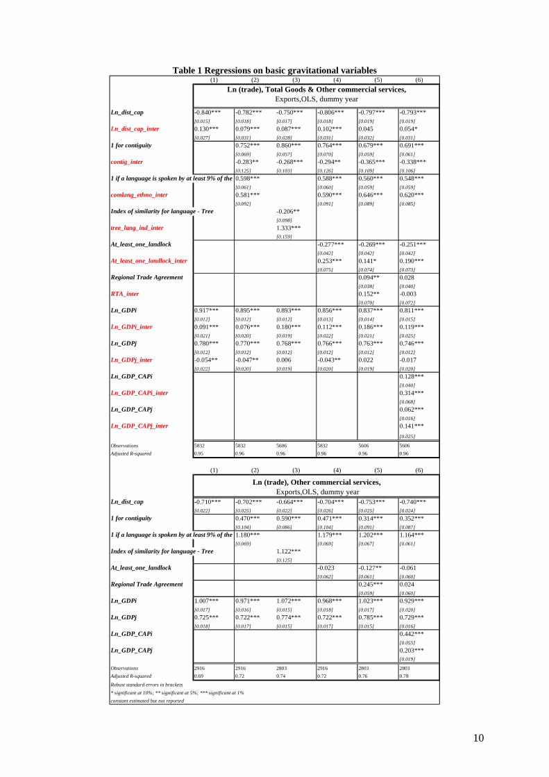
Regressions on Basic Gravitational Variables In Tables 1 to 5 we report the results based on basic gravitational variables. Each table presents a different type of services. Even though we will make reference of some particularities presented in travel and transport services, for the sake of brevity, we will focus on the results for OCS (for the rest, see Tables 2 to 5 in the appendix). All estimated equations are based on Ordinary Least Square. In the upper part of the table we report results of regressing trade in goods and trade in services (pooled) on explanatory variables and on their corresponding interaction term (denoted by the suffix term “_inter” ) ; the bottom part of the table reports results when trade is regressed only for the service sample. In Table 1, it is interesting to remark that the effect of variables related to physical geography (distance, contiguity and landlocked status) is significantly lower when explaining trade in OCS, for all specifications24. In contrast, for language variables, which can be considered as cultural and/or informational proxies, the impact is significantly higher in the case of services. Regarding geographical variables and trade in transportation and travel services, it is not surprising that findings in OCS do not necessarily apply. For instance, the impact of the landlocked status variable is more important in the case of transportation services than in

22 (i.e. Total Services, Other Commercial Services, Travel, Transportation, and Government Services). 23 We focus on trade in OCS since: (1) it has been the most dynamic sector in service trade (2) and also because previous literature has centered their attention on intermediate services (mostly included in Other Commercial Services). 24 With the sole exception of distance in column (5).

9

goods, because countries without sea access simply could not offer maritime transport services25. Finally the variable contiguity does not seem to have a different effect in travel and in trade in goods. The differential effect of GDP per capita on trade in OCS is positive and significant for both exporting and importing countries. This is not astonishing in the case of the exporting country, as we know that the contribution of service activity depends on the level of country development26. However, it is less evident for the importing case. Two possible explanations can arise: (1) specialized OCS might require a more sophisticated target market able to consume complex services and (2) trade in services can only occur if inputs from both trading countries are jointly used in the process27 as suggested by Mirza et al (2006). These findings also show up in Transportation services (GDP per cap. can be reflecting transportation infrastructure in both partner countries) but not in the case of travel where coefficient of GDP per capita of the exporting country is even negative28. Concerning the incremental effect of GDP on OCS, it is always positive and significant for the exporting country case29. In the case of importing country variable, there is no clear pattern. Participation in a Regional Trade Agreement shows up to be more important for trade in OCS than for trade in goods (column 5) but its impact in trade in goods and trade in services becomes non significant when the GDP per capita variable is included (column 6)30. Finally the incremental impact of this variable performs very differently when regressing travel and transportation trade, being positive and significant for the first and negative for the second.

25 In the case of trade in goods, by contrast, when at least one of partner countries has a landlocked status the transportation cost of trading goods is more expensive but it is not prohibitive. 26 That is not the case for Industry and Agricultural sectors as we show in the Figure 1. 27 Think about exports in complex software packages (e.g. Oracle and SAP) which are commercialised by a consulting firm in the importing country. Then, specialised computer skills are required in both the exporting and importing country in order to software exportation to occur. 28 A possible explanation for this result is tourism to low-cost destinations in developing countries. 29 This can be reflecting presence of IRS. Service firms from big domestic markets might benefit of economic advantages at the moment of entering in international markets. 30 A possible explanation for this result is that RTA participation can be correlated to the level of development.

10

Table 1 Regressions on basic gravitational variables (1) (2) (3) (4) (5) (6)

Ln_dist_cap -0.840*** -0.782*** -0.750*** -0.806*** -0.797*** -0.793 ***[0.015] [0.018] [0.017] [0.018] [0.019] [0.019]

Ln_dist_cap_inter 0.130*** 0.079*** 0.087*** 0.102*** 0.045 0.054*[0.027] [0.031] [0.028] [0.031] [0.032] [0.031]

1 for contiguity 0.752*** 0.860*** 0.764*** 0.679*** 0.691***[0.069] [0.057] [0.070] [0.059] [0.061]

contig_inter -0.283** -0.268*** -0.294** -0.365*** -0.338***[0.125] [0.103] [0.126] [0.109] [0.106]

1 if a language is spoken by at least 9% of the population in both countries0.598*** 0.588*** 0.560*** 0.548***[0.061] [0.060] [0.059] [0.059]

comlang_ethno_inter 0.581*** 0.590*** 0.646*** 0.620***[0.092] [0.091] [0.089] [0.085]

Index of similarity for language - Tree -0.206**[0.098]

tree_lang_ind_inter 1.333***[0.159]

At_least_one_landlock -0.277*** -0.269*** -0.251***[0.042] [0.042] [0.042]

At_least_one_landlock_inter 0.253*** 0.141* 0.190***[0.075] [0.074] [0.073]

Regional Trade Agreement 0.094** 0.028[0.038] [0.040]

RTA_inter 0.152** -0.003[0.070] [0.072]

Ln_GDPi 0.917*** 0.895*** 0.893*** 0.856*** 0.837*** 0.811***[0.012] [0.012] [0.012] [0.013] [0.014] [0.015]

Ln_GDPi_inter 0.091*** 0.076*** 0.180*** 0.112*** 0.186*** 0.119***[0.021] [0.020] [0.019] [0.022] [0.021] [0.025]

Ln_GDPj 0.780*** 0.770*** 0.768*** 0.766*** 0.763*** 0.746***[0.012] [0.012] [0.012] [0.012] [0.012] [0.012]

Ln_GDPj_inter -0.054** -0.047** 0.006 -0.043** 0.022 -0.017[0.022] [0.020] [0.019] [0.020] [0.019] [0.020]

Ln_GDP_CAPi 0.128***[0.040]

Ln_GDP_CAPi_inter 0.314***[0.068]

Ln_GDP_CAPj 0.062***[0.016]

Ln_GDP_CAPj_inter 0.141***

[0.025]

Observations 5832 5832 5606 5832 5606 5606

Adjusted R-squared 0.95 0.96 0.96 0.96 0.96 0.96

(1) (2) (3) (4) (5) (6)

Ln_dist_cap -0.710*** -0.702*** -0.664*** -0.704*** -0.753*** -0.740 ***[0.022] [0.025] [0.022] [0.026] [0.025] [0.024]

1 for contiguity 0.470*** 0.590*** 0.471*** 0.314*** 0.352***[0.104] [0.086] [0.104] [0.091] [0.087]


Index of similarity for language - Tree 1.122***[0.125]

At_least_one_landlock -0.023 -0.127** -0.061[0.062] [0.061] [0.060]

Regional Trade Agreement 0.245*** 0.024[0.059] [0.060]

Ln_GDPi 1.007*** 0.971*** 1.072*** 0.968*** 1.023*** 0.929***[0.017] [0.016] [0.015] [0.018] [0.017] [0.020]

Ln_GDPj 0.725*** 0.722*** 0.774*** 0.722*** 0.785*** 0.729***[0.018] [0.017] [0.015] [0.017] [0.015] [0.016]

Ln_GDP_CAPi 0.442***[0.055]

Ln_GDP_CAPj 0.203***[0.019]

Observations 2916 2916 2803 2916 2803 2803


Robust standard errors in brackets

* significant at 10%; ** significant at 5%; *** significant at 1%

constant estimated but not reported

Ln (trade), Total Goods & Other commercial services,Exports,OLS, dummy year

Ln (trade), Other commercial services, Exports,OLS, dummy year

11

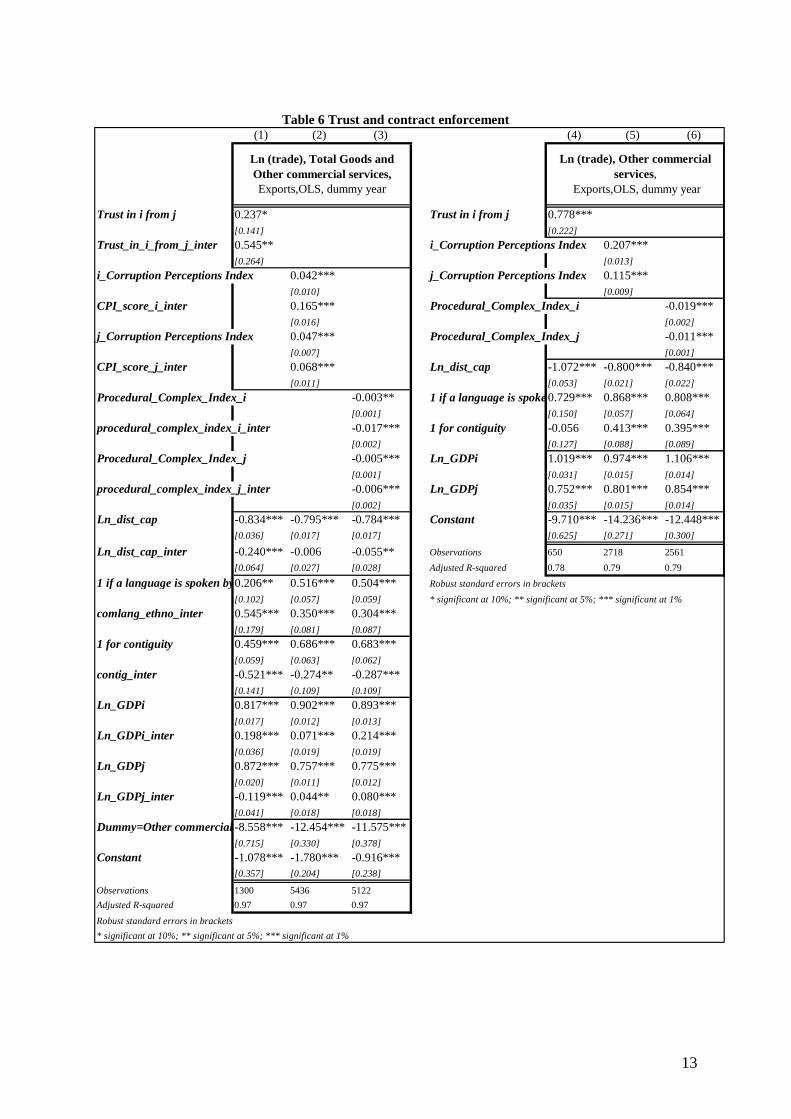
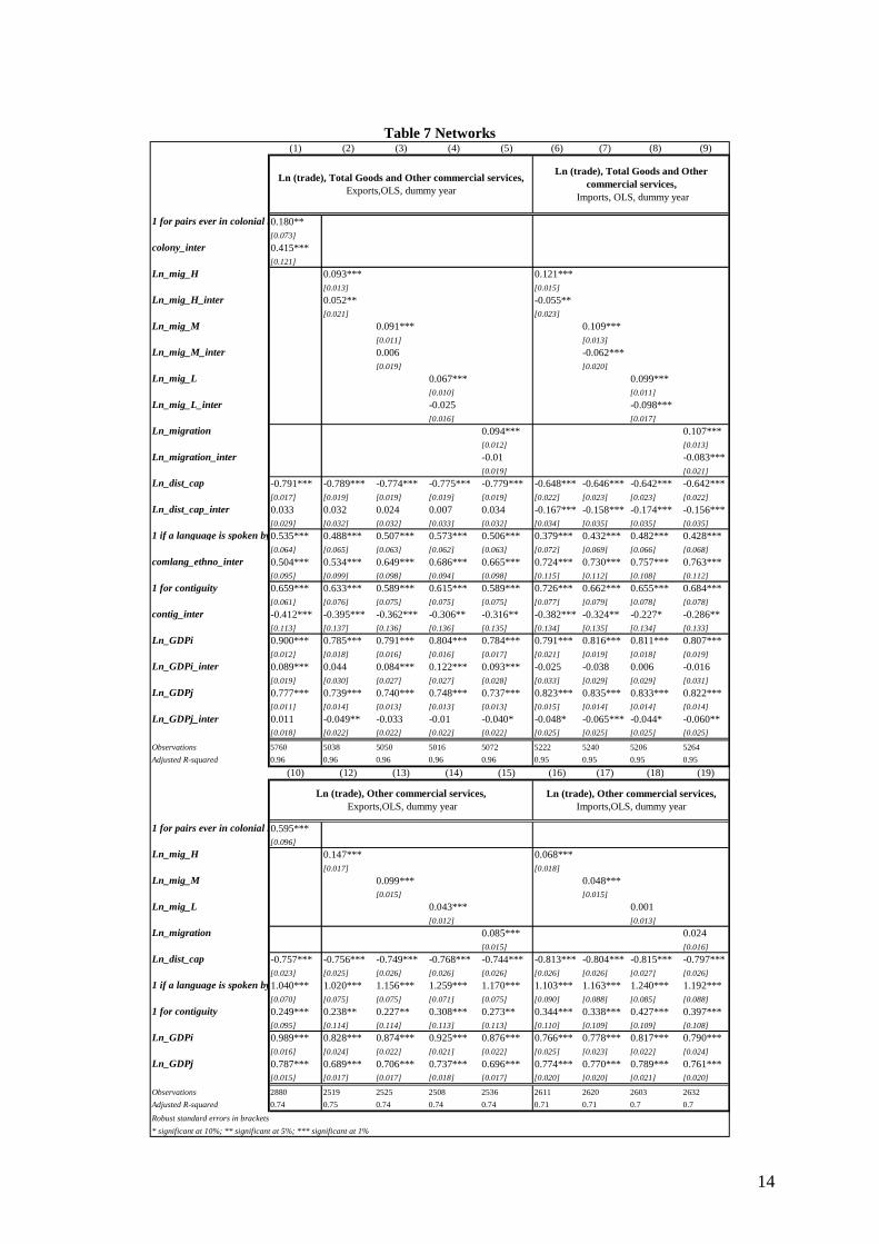
Testing Particular Aspects of Trade in Other Commercial Services Tables 5 to 9 report results of regressions for trade in OCS on: Trust and contract enforcement (Table 6), Networks (Table 7), Labor market (Table 8) and Technology and technology of communication (Table 9).As in the previous section each table presents results of both the pooled sample (trade in goods and trade in services) and the OCS sample. Results in Table 6 show us that variables explaining trust and contract enforcement environments are consistently more important in the case of OCS. This is consistent with the hypothesis that services contract is a risky experience and that existence of secure environments might have a higher impact on business services sector than on manufacture sector. Table 7 reports results in the effect of Networks. As expected, the fact that the pair of countries has ever been in a colonial relationship has a higher impact for the trade in services than for the case of trade in goods. Additionally, and as literature suggest, Networks can promote trade through two main economic mechanisms: First, Networks can reduce information costs as immigrants know the characteristics of many domestic buyers and sellers and carry this knowledge abroad (Rauch 2001) and second, Networks can act as a diffusion agent of preferences. Presence of foreigners can raise imports from origin countries both because migrants bring their tastes for home goods and because nationals partly could acquire a taste for those new varieties (Combes et al. 2005). Presumably, informational channel takes place mainly through the impact of immigrants on exports since they may influence creation of new business between their host country and their country of origin. By contrast, preference effect mainly takes place by the impact of immigrants on imports, as immigrants stimulate consumption of goods from their home countries31.We expect that in the case of more differentiated products (i.e. OCS) the networks as information mechanism should prevail, while in the case of product having “reference prices” (i.e. Goods) the preference mechanism should be more important. Therefore, immigrants must have a bigger impact on exports in the case of OCS than in the case of goods (and a comparatively lower impact when analyzing imports). Our findings seem to follow this pattern. For all migration variables, the impact of migration on trade in OCS is more important for exporting regressions (column 2-5, bottom, Table 7) than in the case of imports (column 6-9).The contrary happens for the trade in goods. It is interesting to remark that the positive effect of migrations on trade increases with the level of education of migrants for both trade in goods and trade in OCS, but it is in the last case where the impact increases the most. Doubling highly qualified migrants in the host country increases the exports of services in 14.7 percent, and in 9.3 percent for the case of exported goods. When considering migrants with low level of education the effects are 4.3 percent and 6.7 percent respectively32.

31 As suggested by Rauch (2001), reciprocal knowledge of trade partners of a same Network can reduce opportunism in business; consequently networks can act as substitutes of contract enforcement laws. 32 However, results might be considered with caution because of the potential existence of reverse causality. Migrants could be more attracted to host countries with large services sectors (hence, potentially strong exporters of services), to the extent that the bigger the services sector is, the higher the work opportunities in services sector are.

12

In the same line and for the export case, the differential effect is positive and significant for highly educated migrants. As the level of education decreases, the differential effect also decreases; even it becomes negative, yet non significant, for migrants with low levels of education. For the case of imports the differential effect is always negative and significant, but their negative effect decreases with the level of education. Results in Table 8 suggest that educational attainment and freedom in labor markets have a higher impact on trade in OCS than on trade in goods. The average schooling years in both exporting and importing country has a significant higher impact on OCS than on trade in goods. Attaining an additional schooling year in the exporting country leads to an increase of exports in OCS by a 17.35 percent and to an increase of exported goods by a 7.35 percent33. Regarding the variables by level of education, the same pattern founded in the case of the migrant variables applies. In the case of population with the highest level of education the differential effect is positive and significant. As the level of education decreases, the differential effect also decreases, becoming even significantly negative for the bottom level of education34. We found that rigidities in country’s labor market, in both exporter and importer countries, have a higher impact on trade in OCS than on trade in goods. Finally and as shown in Table 9, the incremental effect, for all our “technological environment” variables are always positive and statistically significant, which supports the argument that technological advances are more influential on services trade since they have allowed original non-tradable services to become tradable.

33 Here again, the coefficients must be considered with caution because of potential problems of endogeneity. Maybe, the existence of a dynamic service sector can also act as a private incentive to invest in education. 34 See for instance the case of the population with the highest level of education for the trade in goods (column 2). The coefficient for the exporting country is negative (and for the importing country is non significant). By contrast they are positive and highly significant for both countries in the case of services trade (column 7).

13

Table 6 Trust and contract enforcement

(1) (2) (3) (4) (5) (6)

Trust in i from j 0.237* Trust in i from j 0.778***[0.141] [0.222]

Trust_in_i_from_j_inter 0.545** i_Corruption Perceptions Index 0.207***[0.264] [0.013]

i_Corruption Perceptions Index 0.042*** j_Corruption Perceptions Index 0.115***[0.010] [0.009]

CPI_score_i_inter 0.165*** Procedural_Complex_Index_i -0.019***[0.016] [0.002]

j_Corruption Perceptions Index 0.047*** Procedural_Complex_Index_j -0.011***[0.007] [0.001]

CPI_score_j_inter 0.068*** Ln_dist_cap -1.072*** -0.800*** -0.840***[0.011] [0.053] [0.021] [0.022]

Procedural_Complex_Index_i -0.003** 1 if a language is spoken by at least 9% of the population in both countries0.729*** 0.868*** 0.808***[0.001] [0.150] [0.057] [0.064]

procedural_complex_index_i_inter -0.017*** 1 for contiguity -0.056 0.413*** 0.395***[0.002] [0.127] [0.088] [0.089]

Procedural_Complex_Index_j -0.005*** Ln_GDPi 1.019*** 0.974*** 1.106***[0.001] [0.031] [0.015] [0.014]

procedural_complex_index_j_inter -0.006*** Ln_GDPj 0.752*** 0.801*** 0.854***[0.002] [0.035] [0.015] [0.014]

Ln_dist_cap -0.834*** -0.795*** -0.784*** Constant -9.710*** -14.236*** -12.448***[0.036] [0.017] [0.017] [0.625] [0.271] [0.300]

Ln_dist_cap_inter -0.240*** -0.006 -0.055** Observations 650 2718 2561

[0.064] [0.027] [0.028] Adjusted R-squared 0.78 0.79 0.79

1 if a language is spoken by at least 9% of the population in both countries0.206** 0.516*** 0.504*** Robust standard errors in brackets

[0.102] [0.057] [0.059] * significant at 10%; ** significant at 5%; *** significant at 1%

comlang_ethno_inter 0.545*** 0.350*** 0.304***[0.179] [0.081] [0.087]

1 for contiguity 0.459*** 0.686*** 0.683***[0.059] [0.063] [0.062]

contig_inter -0.521*** -0.274** -0.287***[0.141] [0.109] [0.109]

Ln_GDPi 0.817*** 0.902*** 0.893***[0.017] [0.012] [0.013]

Ln_GDPi_inter 0.198*** 0.071*** 0.214***[0.036] [0.019] [0.019]

Ln_GDPj 0.872*** 0.757*** 0.775***[0.020] [0.011] [0.012]

Ln_GDPj_inter -0.119*** 0.044** 0.080***[0.041] [0.018] [0.018]

Dummy=Other commercial services-8.558*** -12.454*** -11.575***[0.715] [0.330] [0.378]

Constant -1.078*** -1.780*** -0.916***[0.357] [0.204] [0.238]

Observations 1300 5436 5122

Adjusted R-squared 0.97 0.97 0.97



Ln (trade), Total Goods and Other commercial services, Exports,OLS, dummy year

Ln (trade), Other commercial services,

Exports,OLS, dummy year

14

Table 7 Networks

(1) (2) (3) (4) (5) (6) (7) (8) (9)

1 for pairs ever in colonial relationship0.180**[0.073]

colony_inter 0.415***[0.121]

Ln_mig_H 0.093*** 0.121***[0.013] [0.015]

Ln_mig_H_inter 0.052** -0.055**[0.021] [0.023]

Ln_mig_M 0.091*** 0.109***[0.011] [0.013]

Ln_mig_M_inter 0.006 -0.062***[0.019] [0.020]

Ln_mig_L 0.067*** 0.099***[0.010] [0.011]

Ln_mig_L_inter -0.025 -0.098***[0.016] [0.017]

Ln_migration 0.094*** 0.107***[0.012] [0.013]

Ln_migration_inter -0.01 -0.083***[0.019] [0.021]

Ln_dist_cap -0.791*** -0.789*** -0.774*** -0.775*** -0.779*** -0.648 *** -0.646*** -0.642*** -0.642***[0.017] [0.019] [0.019] [0.019] [0.019] [0.022] [0.023] [0.023] [0.022]

Ln_dist_cap_inter 0.033 0.032 0.024 0.007 0.034 -0.167*** -0.158*** -0.174*** -0.156***[0.029] [0.032] [0.032] [0.033] [0.032] [0.034] [0.035] [0.035] [0.035]

1 if a language is spoken by at least 9% of the population in both countries0.535*** 0.488*** 0.507*** 0.573*** 0.506*** 0.379*** 0.4 32*** 0.482*** 0.428***[0.064] [0.065] [0.063] [0.062] [0.063] [0.072] [0.069] [0.066] [0.068]

comlang_ethno_inter 0.504*** 0.534*** 0.649*** 0.686*** 0.665*** 0.724*** 0.7 30*** 0.757*** 0.763***[0.095] [0.099] [0.098] [0.094] [0.098] [0.115] [0.112] [0.108] [0.112]

1 for contiguity 0.659*** 0.633*** 0.589*** 0.615*** 0.589*** 0.726*** 0.6 62*** 0.655*** 0.684***[0.061] [0.076] [0.075] [0.075] [0.075] [0.077] [0.079] [0.078] [0.078]

contig_inter -0.412*** -0.395*** -0.362*** -0.306** -0.316** -0.382** * -0.324** -0.227* -0.286**[0.113] [0.137] [0.136] [0.136] [0.135] [0.134] [0.135] [0.134] [0.133]

Ln_GDPi 0.900*** 0.785*** 0.791*** 0.804*** 0.784*** 0.791*** 0.8 16*** 0.811*** 0.807***[0.012] [0.018] [0.016] [0.016] [0.017] [0.021] [0.019] [0.018] [0.019]

Ln_GDPi_inter 0.089*** 0.044 0.084*** 0.122*** 0.093*** -0.025 -0.038 0.006 -0.016[0.019] [0.030] [0.027] [0.027] [0.028] [0.033] [0.029] [0.029] [0.031]

Ln_GDPj 0.777*** 0.739*** 0.740*** 0.748*** 0.737*** 0.823*** 0.8 35*** 0.833*** 0.822***[0.011] [0.014] [0.013] [0.013] [0.013] [0.015] [0.014] [0.014] [0.014]

Ln_GDPj_inter 0.011 -0.049** -0.033 -0.01 -0.040* -0.048* -0.065*** -0.044* -0.060**[0.018] [0.022] [0.022] [0.022] [0.022] [0.025] [0.025] [0.025] [0.025]

Observations 5760 5038 5050 5016 5072 5222 5240 5206 5264

Adjusted R-squared 0.96 0.96 0.96 0.96 0.96 0.95 0.95 0.95 0.95

(10) (12) (13) (14) (15) (16) (17) (18) (19)

1 for pairs ever in colonial relationship0.595***[0.096]

Ln_mig_H 0.147*** 0.068***[0.017] [0.018]

Ln_mig_M 0.099*** 0.048***[0.015] [0.015]

Ln_mig_L 0.043*** 0.001[0.012] [0.013]

Ln_migration 0.085*** 0.024[0.015] [0.016]

Ln_dist_cap -0.757*** -0.756*** -0.749*** -0.768*** -0.744*** -0.813 *** -0.804*** -0.815*** -0.797***[0.023] [0.025] [0.026] [0.026] [0.026] [0.026] [0.026] [0.027] [0.026]

1 if a language is spoken by at least 9% of the population in both countries1.040*** 1.020*** 1.156*** 1.259*** 1.170*** 1.103*** 1.1 63*** 1.240*** 1.192***[0.070] [0.075] [0.075] [0.071] [0.075] [0.090] [0.088] [0.085] [0.088]

1 for contiguity 0.249*** 0.238** 0.227** 0.308*** 0.273** 0.344*** 0.338*** 0.427*** 0.397***[0.095] [0.114] [0.114] [0.113] [0.113] [0.110] [0.109] [0.109] [0.108]

Ln_GDPi 0.989*** 0.828*** 0.874*** 0.925*** 0.876*** 0.766*** 0.7 78*** 0.817*** 0.790***[0.016] [0.024] [0.022] [0.021] [0.022] [0.025] [0.023] [0.022] [0.024]

Ln_GDPj 0.787*** 0.689*** 0.706*** 0.737*** 0.696*** 0.774*** 0.7 70*** 0.789*** 0.761***[0.015] [0.017] [0.017] [0.018] [0.017] [0.020] [0.020] [0.021] [0.020]

Observations 2880 2519 2525 2508 2536 2611 2620 2603 2632

Adjusted R-squared 0.74 0.75 0.74 0.74 0.74 0.71 0.71 0.7 0.7




Ln (trade), Total Goods and Other commercial services,

Imports, OLS, dummy year


Ln (trade), Other commercial services, Imports,OLS, dummy year

15

Table 8 Labor markets (1) (2) (3) (4) (5) (6) (7) (8) (9) (10)

years_edu_i 0.071*** years_edu_i 0.160***[0.011] [0.013]

years_edu_i_inter 0.089*** years_edu_j 0.093***[0.017] [0.010]

years_edu_j 0.039*** high_edu_i 0.009***[0.008] [0.002]

years_edu_j_inter 0.055*** high_edu_j 0.011***[0.013] [0.002]

high_edu_i -0.004** second_edu_i 0.023***[0.002] [0.002]

high_edu_i_inter 0.013*** second_edu_j 0.017***[0.003] [0.002]

high_edu_j 0.001 prim_edu_i -0.019***[0.002] [0.002]

high_edu_j_inter 0.010*** prim_edu_j -0.014***[0.003] [0.002]

second_edu_i 0.019*** Empl_Laws_Index_i -0.016***[0.002] [0.002]

second_edu_i_inter 0.004 Empl_Laws_Index_j -0.018***[0.003] [0.001]

second_edu_j 0.008*** Ln_dist_cap -0.850*** -0.870*** -0.770*** -0.871*** -0.810***[0.001] [0.024] [0.027] [0.025] [0.025] [0.021]

second_edu_j_inter 0.009*** 1 if a language is spoken by at least 9% of the population in both countries0.912*** 1.007*** 1.240*** 0.970*** 0.745***[0.002] [0.070] [0.075] [0.067] [0.072] [0.060]

prim_edu_i -0.012*** 1 for contiguity -0.033 0.005 -0.111 -0.075 0.378***[0.002] [0.100] [0.105] [0.100] [0.099] [0.091]

prim_edu_i_inter -0.007*** Ln_GDPi 1.038*** 1.047*** 1.038*** 1.008*** 1.039***[0.002] [0.017] [0.018] [0.017] [0.017] [0.015]

prim_edu_j -0.002 Ln_GDPj 0.718*** 0.728*** 0.727*** 0.724*** 0.844***[0.001] [0.017] [0.018] [0.017] [0.017] [0.014]

prim_edu_j_inter -0.013*** Constant -13.495*** -11.728*** -13.615*** -9.625*** -11.720***[0.002] [0.361] [0.372] [0.366] [0.407] [0.324]

Empl_Laws_Index_i -0.002* Observations 2064 2064 2064 2064 2561

[0.001] Adjusted R-squared 0.78 0.76 0.78 0.77 0.79

empl_laws_index_i_inter -0.013*** Robust standard errors in brackets

[0.002] * significant at 10%; ** significant at 5%; *** significant at 1%

Empl_Laws_Index_j -0.009***[0.001]

empl_laws_index_j_inter -0.009***[0.002]

Ln_dist_cap -0.791*** -0.775*** -0.746*** -0.805*** -0.784***[0.018] [0.019] [0.019] [0.018] [0.016]

Ln_dist_cap_inter -0.059* -0.095*** -0.024 -0.066** -0.025[0.031] [0.033] [0.031] [0.031] [0.027]

1 if a language is spoken by at least 9% of the population in both countries0.506*** 0.655*** 0.691*** 0.547*** 0.445***[0.063] [0.068] [0.060] [0.064] [0.058]

comlang_ethno_inter 0.407*** 0.353*** 0.550*** 0.424*** 0.303***[0.094] [0.101] [0.090] [0.096] [0.083]

1 for contiguity 0.414*** 0.428*** 0.352*** 0.389*** 0.678***[0.060] [0.064] [0.064] [0.060] [0.063]

contig_inter -0.447*** -0.423*** -0.463*** -0.465*** -0.299***[0.117] [0.123] [0.119] [0.116] [0.111]

Ln_GDPi 0.884*** 0.901*** 0.873*** 0.858*** 0.885***[0.014] [0.015] [0.014] [0.014] [0.013]

Ln_GDPi_inter 0.154*** 0.146*** 0.166*** 0.151*** 0.154***[0.022] [0.023] [0.022] [0.023] [0.019]

Ln_GDPj 0.719*** 0.730*** 0.720*** 0.732*** 0.766***[0.014] [0.015] [0.013] [0.014] [0.012]

Ln_GDPj_inter 0 -0.002 0.007 -0.008 0.078***[0.022] [0.023] [0.022] [0.022] [0.018]

Dummy=Other commercial services-12.188*** -10.944*** -11.971*** -10.040*** -11.250***[0.460] [0.471] [0.468] [0.521] [0.415]

Constant -1.362*** -0.829*** -1.702*** 0.365 -0.556**[0.296] [0.296] [0.301] [0.330] [0.269]

Observations 4128 4128 4128 4128 5122

Adjusted R-squared 0.97 0.96 0.97 0.97 0.97





16

Table 9 Technology and technology of communication (1) (2) (3) (4) (5) (6) (7) (8) (9) (10)

Ln_PCs_i 0.297*** Ln_PCs_i 0.855***[0.035] [0.044]

Ln_PCs_i_inter 0.549*** Ln_PCs_j 0.237***[0.056] [0.016]

Ln_PCs_j 0.104*** Ln_Internet_users_i 0.610***[0.014] [0.052]

Ln_PCs_j_inter 0.129*** Ln_Internet_users_j 0.224***[0.021] [0.018]

Ln_Internet_users_i 0.309*** Ln_Tele_mainlines_i 1.716***[0.039] [0.120]

Ln_Internet_users_i_inter 0.272*** Ln_Tele_mainlines_j 0.290***[0.061] [0.030]

Ln_Internet_users_j 0.129*** Ln_internet_hosts_1_i 0.304***[0.014] [0.037]

Ln_Internet_users_j_inter 0.087*** Ln_internet_hosts_1_j 0.104***[0.023] [0.014]

Ln_Tele_mainlines_i -0.224*** R&D_i (% of GDP) 0.281***[0.085] [0.037]

Ln_Tele_mainlines_i_inter 1.943*** R&D_j (% of GDP) 0.062**[0.147] [0.026]

Ln_Tele_mainlines_j 0.098*** Ln_dist_cap -0.775*** -0.727*** -0.671*** -0.709*** -0.829***[0.024] [0.021] [0.025] [0.025] [0.036] [0.027]

Ln_Tele_mainlines_j_inter 0.192*** 1 if a language is spoken by at least 9% of the population in both countries0.955*** 1.107*** 1.179*** 0.965*** 1.155***[0.038] [0.061] [0.067] [0.065] [0.091] [0.081]

Ln_internet_hosts_1_i 0.170*** 1 for contiguity 0.336*** 0.430*** 0.538*** 0.485*** 0.288***[0.028] [0.082] [0.095] [0.099] [0.146] [0.098]

Ln_internet_hosts_1_i_inter 0.121*** Ln_GDPi 0.881*** 0.909*** 0.855*** 0.986*** 0.983***[0.045] [0.015] [0.017] [0.017] [0.022] [0.020]

Ln_internet_hosts_1_j 0.062*** Ln_GDPj 0.739*** 0.699*** 0.696*** 0.696*** 0.835***[0.011] [0.015] [0.017] [0.017] [0.025] [0.017]

Ln_internet_hosts_1_j_inter 0.041** Constant -16.074*** -14.699*** -22.620*** -13.621*** -13.022***[0.018] [0.293] [0.333] [0.714] [0.413] [0.310]

R&D_i (% of GDP) 0.202*** Observations 2839 2733 2901 1293 1845

[0.024] Adjusted R-squared 0.79 0.75 0.75 0.77 0.79

R_D_i_inter 0.076* Robust standard errors in brackets

[0.044] * significant at 10%; ** significant at 5%; *** significant at 1%

R&D_j (% of GDP) -0.01[0.017]

R_D_j_inter 0.070**[0.031]

Ln_dist_cap -0.788*** -0.785*** -0.753*** -0.772*** -0.841***[0.017] [0.018] [0.019] [0.027] [0.021]

Ln_dist_cap_inter 0.014 0.059* 0.082*** 0.063 0.013[0.026] [0.030] [0.031] [0.045] [0.034]

1 if a language is spoken by at least 9% of the population in both countries0.494*** 0.524*** 0.599*** 0.494*** 0.547***[0.058] [0.061] [0.060] [0.084] [0.067]

comlang_ethno_inter 0.467*** 0.591*** 0.580*** 0.481*** 0.609***[0.084] [0.090] [0.088] [0.124] [0.105]

1 for contiguity 0.687*** 0.736*** 0.756*** 0.751*** 0.636***[0.063] [0.071] [0.070] [0.109] [0.066]

contig_inter -0.351*** -0.309*** -0.219* -0.266 -0.347***[0.104] [0.119] [0.121] [0.183] [0.118]

Ln_GDPi 0.860*** 0.857*** 0.916*** 0.856*** 0.829***[0.013] [0.012] [0.013] [0.018] [0.014]

Ln_GDPi_inter 0.025 0.057*** -0.060*** 0.135*** 0.156***[0.020] [0.021] [0.022] [0.028] [0.024]

Ln_GDPj 0.743*** 0.741*** 0.755*** 0.747*** 0.769***[0.011] [0.012] [0.012] [0.018] [0.012]

Ln_GDPj_inter -0.001 -0.039* -0.059*** -0.048 0.068***[0.018] [0.021] [0.021] [0.031] [0.021]

Dummy=Other commercial services-13.598*** -12.105*** -21.906*** -11.936*** -12.758***[0.372] [0.417] [0.877] [0.518] [0.363]

Constant -2.565*** -2.614*** -0.78 -1.758*** -0.366*[0.234] [0.258] [0.511] [0.316] [0.212]

Observations 5678 5466 5802 2586 3690

Adjusted R-squared 0.97 0.96 0.96 0.96 0.97





17

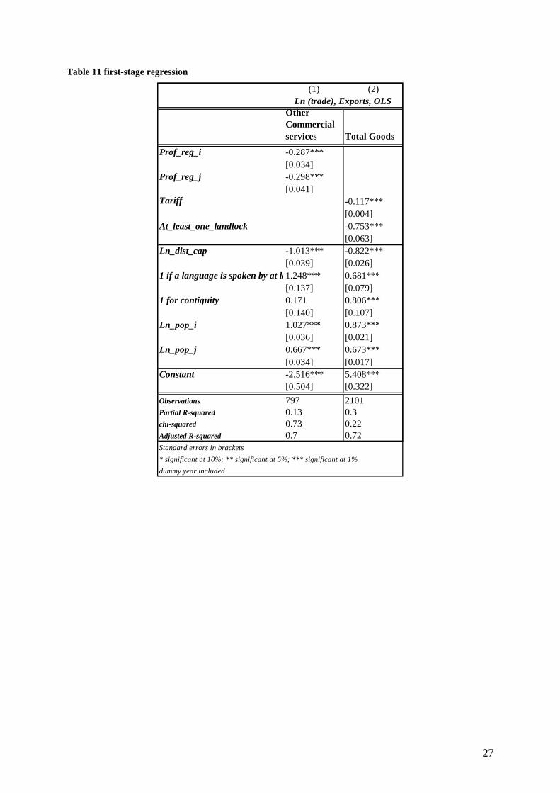
5. Instrumental Variables Estimation As instruments for trade in “Other commercial services” we use data on regulatory conditions in professional services sectors, elaborated by the OECD35. In particular, we use an indicator which summarizes the rigidities that professionals face in order to exercise their occupations. To instrument trade in goods36 we use (1) the average applied import tariff on non-agricultural and non-fuel products37 and (2) the variable indicating if at least one of the two countries has a landlocked status38. The First-Stage regressions perform reasonably well, suggesting that we do not have “weak” instruments problem. Additionally, Sargan tests confirm the validity of our instruments: our instruments for trade in goods are affecting trade in services only through their impact on trade in goods (and vice versa our instruments for trade in services are not affecting independently trade in goods) 39. Table 10 presents results on the implementation of instrumental variables40. The first three columns present regressions of trade in goods: a simple OLS regression is estimated for comparison in column (1). In column (2) we add trade in OCS as explanatory variable using OLS and column (3) presents results when trade in services is instrumented. Columns 4 to 6 repeat the same exercise for regressions explaining trade in “Other commercial services”. The coefficients of our instrumental variables are positive and significant at standard levels. Trade in goods affects strongly trade in services: the estimated elasticity is almost 1, indicating that an increase in “x” percent in trade in goods induces the same percent increase in bilateral trade in services. Reciprocally, trade in OCS affects positively bilateral trade in goods although the effect is less strong (0.458). Regarding the other coefficients it is interesting to remark that: first, once we add trade in services to explain trade in goods, the coefficient of the language variable drastically decreases and even becomes negative (columns (2) and (3)). Second, when we add trade in goods in order to explain trade in OCS, the coefficients of geographical variables (contiguity and distance) decrease even to the limit to reverse their signs (columns (5) and (6)). These results seem to indicate that the effect of cultural and /or informational variables affect positively trade in goods indirectly through their impact on trade in services. Conversely, the effect of the geographical variables affect (in the traditional way) trade in services indirectly through their impact on trade in goods.

35 Conway, P. and G. Nicoletti (2006), "Product market regulation in non-manufacturing sectors: measurement and highlights", OECD Economics Department Working Paper 36 We also use, without success because of endogeneity, (1) the bilateral cost of shipping a ton between the two main cities of the country pair using UPS services, (2) data on average time in clearing exports and (3) data on average time in claiming imports from Enterprise Surveys from World Bank. 37 Data are drawn from UNCTAD Handbook of Statistics On-line. 38 We use population instead GDP to avoid potential problems of collinearity. 39 The Partial-R² is 0.13 for instruments in the case of trade in services; and 0.3 in the case of traded goods. Chi² from Sargan tests are 0.73 and 0.22 respectively. 40 In the Appendix we show the first-stage regressions.

18

Table 10 Instrumental Variables Estimation (1) (2) (3) (4) (5) (6)

Total Goods, Ln (trade), Exports, OLS , dummy year

Total Goods, Ln (trade), Exports, OLS , dummy year

Total Goods, Ln (trade), Exports, IV , dummy year

Other services , Ln (trade), Exports, OLS, dummy year

Other services , Ln (trade), Exports, OLS, dummy year

Other services , Ln (trade), Exports, IV, dummy year

Ln_dist_cap -0.826*** -0.410*** -0.344*** -0.695*** 0.077** 0.086**[0.028] [0.030] [0.060] [0.040] [0.030] [0.038]

1 if a language is spoken by at least 9% of the population in both countries0.226** -0.254*** -0.331*** 1.256*** 0.640*** 0.633***[0.097] [0.082] [0.102] [0.123] [0.082] [0.084]

1 for contiguity0.671*** 0.675*** 0.675*** 0.634*** -0.266** -0.277**[0.099] [0.080] [0.080] [0.167] [0.111] [0.114]

Ln_pop_i 0.781*** 0.400*** 0.340*** 0.963*** 0.047* 0.036[0.025] [0.027] [0.055] [0.030] [0.027] [0.038]

Ln_pop_j 0.669*** 0.443*** 0.406*** 0.506*** -0.051** -0.058**[0.022] [0.021] [0.036] [0.026] [0.020] [0.026]

Ln (Trade in Other Services) 0.395*** 0.458***[0.019] [0.053]

Ln (Trade in Goods) 0.978*** 0.990***[0.019] [0.034]

Constant 6.391*** 7.194*** 7.322*** -4.902*** -9.592*** -9.649***[0.357] [0.291] [0.308] [0.435] [0.301] [0.330]

Observations 797 797 797 2101 2101 2101Adjusted R-squared0.77 0.85 0.46 0.77

Standard errors in brackets* significant at 10%; ** significant at 5%; *** significant at 1%

6. Conclusion Using disaggregate data on trade in services, we have empirically explored, first to what extent trade in services differs from trade in goods and second the existence of complementarity between bilateral trade in goods and bilateral trade in services. We found that the effects of variables related to physical geography (distance, contiguity and landlocked status) are significantly lower when explaining trade in Other Commercial Services. In contrast, for language variables, which can be considered as cultural and/or informational proxies, the impact is significantly higher for the services trade case. Additionally results are consistent with the hypotheses that Trust and contract enforcement, Networks, Countries’ level of education, Labor markets regulation and Technology of communication are more important when explaining trade in Other Commercial Services than when explaining trade in goods. Finally we show in this paper that trade in goods and in Other Commercial Services reinforce each other. Bilateral trade in goods explains bilateral trade in services: the resulting estimated elasticity is close to 1. Reciprocally, bilateral trade in services affects positively bilateral trade in goods: a 10% increase in trade in services raises traded goods by 4.58%.

19

References 1 Amiti M.; S. Wei (October 2004); Fear of Service Outsourcing: Is It Justified?

IMF Working Papers

2 Aviat A. and N. Coeurdacier (2005); The Geography of Trade in Goods and Asset HoldingsForthcoming in the Journal of International Economics.

3 Baier S. and Bergstrand J. (2001). The Growth of World Trade: Tariffs, Transport Costs, and Income Similarity, Journal of International Economics, Vol. 53, pp: 1–27

4 Barro, R.. and J. Lee, (2000); International Data on Educational Attainment: Updates and ImplicationsCID Working Paper No. 42

5 Bhagwati J.; A. Panagariya and T. Srinivasan (August 2004); The Muddles over OutsourcingThe Journal of Economic Perspectives; Vol. 18, Nº 4, pp 93–114

6 Combes P.; M.Lafourcade and T. Maye (2005); The trade-creating effects of business and social networks: evidence from FranceJournal of International Economics; Vol. 66, Issue 1, pp. 1-29

7 Conway, P. and G. Nicoletti (2006), Product market regulation in non-manufacturing sectors: measurement and highlights, OECD Economics Department Working Paper

8 Deardoff A.; D.Brown and R.Stern (1995); Modelling Multilateral Trade Liberalization in ServicesWorking Papers from Michigan - Research Forum on International Economics

9 Deardorff A.; V. and R.Stern (January 2004); Empirical Analysis of Barriers to International Services Transactions and the Consequences of LiberalizationUniversity of Michigan; Discussion Paper No. 505

10 Feenstra R.; G. Hanson, and S. Lin (2004) The Value of Information in International Trade: Gains to Outsourcing through Hong KongAdvances in Economic Analysis & Policy; Vol. 4: No. 1, Article 7.

11 Francois J. and I. Wooton (July 2005); Market Structure in Services and Market Access in GoodsCEPR; Discussion paper N° 5135

12 Freund C., and D. Weinhold (2002); The Internet and International Trade in ServicesAmerican Economic Review; Vol. 92, No.2, pp. 236–40

13 Grünfeld L. and A. Moxnes (2003); The Intangible Globalization: Explaining the Patterns of International Trade in Services Norwegian Institute of International Affairs; Working Paper Nº 657

14 Guiso L.; P. Sapienza and L. Zingales (2005); Cultural Biases in Economic ExchangeCEPR; Discussion paper Nº 4837

15 Helpman, E. and P. Krugman (1985). Market Structure and Foreign Trade: IncreasingReturns, Imperfect Competition and the International Economy, Cambridge, MA: MITPress.

16 Jones R. and H. Kierzkowski (March 2005) International fragmentation and the new economic geographyThe North American Journal of Economics and Finance; Volume 16, Issue 1, pp 1-10

20

17 Jones R., H. Kierzkowski and C. Lurong (2005); What does evidence tell us about fragmentation and outsourcing?International Review of Economics & Finance; Vol. 14, issue 3, pp 305-316

18 Kimura F. and H. Lee (2006); The Gravity Equation in International Trade in ServicesReview of World Economics; Vol. 142, issue 1, pp 92-121

19 Markusen , J.(1989) Trade in producer services and in other specialized Intermediate InputsAmerican Economic Review; Vol. 79, N° 1, 85-85

20 Markusen, J.; T. Rutherford and D.Tarr (August 2000); Foreign Direct Investment in Services and the Domestic Market for ExpertiseWorld Bank, Policy Research Working Paper; Nº 2413

21 Markusen, J.; T. Rutherford and D.Tarr (August 2005); Trade and direct investment in producer services and the domestic market for expertiseCanadian Journal of Economics; Vol. 38, N° 3, pp. 758-777(20)

22 Martin P., T. Mayer and M. Thoenig (September 2005); Make trade not war?CEPR; Discussion paper N° 5218

23 Mirza. D; G. Nicoletti and C. Lennon (2006); Complementarity of Inputs Across Countries in Services Trademimeo

24 Rauch James E.(2001); Business and social networks in international trade Journal of Economic Literature; Vol. 39, Nº 4, pp. 1177– 1203

25 Tinbergen, J. (1962). Shaping the World Economy – Suggestions for an InternationalEconomic Policy, The Twentieth Century Fund.

26 Van Marrewijk C.;J. Stibora and A. de Vaal (November 1996); Services tradability, trade liberalization and Foreign Direct InvestmentEconomica; Vol. 63, Nº 252, pp 611-631

21

Figure 1

Activity's contribution to GDP, 2001Source: World Bank (WDI)

0

10

20

30

40

50

60

70

80

Low income Low er middleincome

Middle income Upper middleincome

World High income

Agriculture, value added (% of GDP) Industry, value added (% of GDP) Services, etc., value added (% of GDP)

Figure 2

22

Figure 3

Share in OECD Total Trade

TOTAL SERVICES 1,250,067 22%

Share in Total Services

Other Commercial Services 600,564 48%

Travel 345,082 28%

Transportation 267,520 21%

Government 36,901 3%

Share in Other Commercial

Services

268: Other business services 278,629 46%

266: Royalties and license fees 81,570 14%

260: Financial services 80,579 13%

262: Computer and information services 43,631 7%

253: Insurance services 41,402 7%

245: Communication services 27,473 5%

249: Construction services 24,672 4%

287: Personal, cultural and recreational services 22,609 4%

Source: OECD Statistics on International Trade in Services

2002 OECD Total Service Exports (Millions of US dollars)

23

Table 2

Ln_dist_cap -0.860*** -0.801*** -0.758*** -0.822*** -0.786*** -0.776 ***[0.016] [0.018] [0.016] [0.018] [0.019] [0.018]

Ln_dist_cap_inter 0.175*** 0.149*** 0.133*** 0.170*** 0.092*** 0.108***[0.026] [0.029] [0.026] [0.030] [0.030] [0.028]

1 for contiguity 0.757*** 0.961*** 0.774*** 0.727*** 0.754***[0.075] [0.065] [0.074] [0.066] [0.071]

contig_inter -0.135 -0.241** -0.151 -0.311*** -0.281**[0.126] [0.108] [0.125] [0.118] [0.117]



Index of similarity for language - Tree -0.309***[0.100]


At_least_one_landlock -0.232*** -0.188*** -0.099**[0.043] [0.042] [0.044]

At_least_one_landlock_inter 0.229*** 0.097 0.151**[0.071] [0.070] [0.068]


RTA_inter 0.278*** 0.119*[0.063] [0.065]

Ln_GDPi 0.952*** 0.927*** 0.914*** 0.890*** 0.856*** 0.786***[0.013] [0.013] [0.012] [0.014] [0.014] [0.015]

Ln_GDPi_inter 0.004 -0.013 0.088*** 0.024 0.099*** 0.046*[0.021] [0.021] [0.020] [0.023] [0.022] [0.024]

Ln_GDPj 0.817*** 0.802*** 0.789*** 0.800*** 0.779*** 0.747***[0.012] [0.012] [0.011] [0.012] [0.011] [0.012]

Ln_GDPj_inter -0.053*** -0.053*** 0.034* -0.051*** 0.038** -0.008[0.020] [0.019] [0.018] [0.019] [0.017] [0.018]

Ln_GDP_CAPi 0.325***[0.038]


Ln_GDP_CAPj 0.126***[0.015]

Ln_GDP_CAPj_inter 0.166***

[0.023]

Observations 7164 7164 6844 7164 6844 6844


(1) (2) (3) (4) (5) (6)

Ln_dist_cap -0.684*** -0.651*** -0.625*** -0.652*** -0.694*** -0.668 ***[0.020] [0.023] [0.020] [0.023] [0.023] [0.022]

1 for contiguity 0.623*** 0.719*** 0.623*** 0.415*** 0.473***[0.101] [0.086] [0.101] [0.098] [0.093]



At_least_one_landlock -0.004 -0.09 0.053[0.057] [0.056] [0.052]

Regional Trade Agreement 0.411*** 0.127**[0.050] [0.050]

Ln_GDPi 0.958*** 0.916*** 1.001*** 0.915*** 0.955*** 0.831***[0.017] [0.017] [0.016] [0.018] [0.017] [0.018]

Ln_GDPj 0.764*** 0.749*** 0.823*** 0.748*** 0.817*** 0.739***[0.016] [0.015] [0.013] [0.015] [0.013] [0.014]

Ln_GDP_CAPi 0.574***[0.048]

Ln_GDP_CAPj 0.293***[0.018]

Observations 3582 3582 3422 3582 3422 3422





Ln (trade), Total Goods &Total Services, Exports,OLS, dummy year

Ln (trade), Total Services, Exports,OLS, dummy year

24

Table 3

Ln_dist_cap -0.796*** -0.723*** -0.701*** -0.745*** -0.727*** -0.719 ***[0.015] [0.017] [0.017] [0.018] [0.019] [0.019]

Ln_dist_cap_inter 0.248*** 0.207*** 0.225*** 0.179*** 0.115*** 0.125***[0.027] [0.031] [0.030] [0.031] [0.034] [0.033]

1 for contiguity 0.846*** 0.986*** 0.857*** 0.793*** 0.825***[0.070] [0.064] [0.070] [0.063] [0.067]

contig_inter -0.278** -0.296*** -0.264** -0.348*** -0.311***[0.120] [0.110] [0.118] [0.113] [0.113]



Index of similarity for language - Tree -0.316***[0.101]



At_least_one_landlock_inter -0.287*** -0.332*** -0.267***[0.074] [0.076] [0.076]


RTA_inter -0.028 -0.146**[0.070] [0.071]

Ln_GDPi 0.888*** 0.859*** 0.873*** 0.830*** 0.817*** 0.778***[0.012] [0.012] [0.012] [0.013] [0.014] [0.015]

Ln_GDPi_inter -0.038* -0.052*** -0.018 -0.088*** -0.054** -0.101***[0.020] [0.020] [0.020] [0.022] [0.022] [0.026]

Ln_GDPj 0.774*** 0.759*** 0.757*** 0.757*** 0.748*** 0.723***[0.012] [0.011] [0.011] [0.011] [0.011] [0.012]

Ln_GDPj_inter -0.052*** -0.047** -0.011 -0.049*** 0.006 -0.023[0.020] [0.019] [0.019] [0.019] [0.019] [0.020]

Ln_GDP_CAPi 0.225***[0.040]


Ln_GDP_CAPj 0.103***[0.015]

Ln_GDP_CAPj_inter 0.119***[0.026]

Observations 6348 6348 6162 6348 6162 6162


(1) (2) (3) (4) (5) (6)

Ln_dist_cap -0.548*** -0.515*** -0.477*** -0.566*** -0.613*** -0.594 ***[0.023] [0.026] [0.025] [0.026] [0.029] [0.027]

1 for contiguity 0.568*** 0.690*** 0.593*** 0.444*** 0.514***[0.097] [0.089] [0.095] [0.093] [0.090]




Regional Trade Agreement 0.103* -0.114*[0.058] [0.059]

Ln_GDPi 0.849*** 0.806*** 0.854*** 0.742*** 0.763*** 0.677***[0.017] [0.016] [0.017] [0.018] [0.018] [0.021]

Ln_GDPj 0.722*** 0.711*** 0.746*** 0.708*** 0.754*** 0.701***[0.016] [0.015] [0.015] [0.015] [0.015] [0.016]

Ln_GDP_CAPi 0.496***[0.062]

Ln_GDP_CAPj 0.222***[0.021]

Observations 3174 3174 3081 3174 3081 3081





Ln (trade), Total Goods & Transportation, Exports,OLS, dummy year

Ln (trade), Transportation, Exports,OLS, dummy year

25

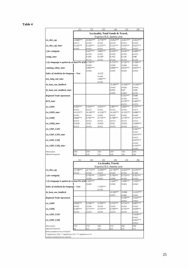
Table 4

(1) (2) (3) (4) (5) (6)

Ln_dist_cap -0.880*** -0.833*** -0.776*** -0.852*** -0.815*** -0.819 ***[0.017] [0.018] [0.019] [0.019] [0.021] [0.020]

Ln_dist_cap_inter 0.132*** 0.120*** 0.215*** 0.121*** 0.163*** 0.221***[0.029] [0.031] [0.031] [0.032] [0.037] [0.035]

1 for contiguity 0.627*** 0.883*** 0.628*** 0.634*** 0.680***[0.070] [0.070] [0.069] [0.070] [0.072]

contig_inter 0.163 0.219* 0.163 0.118 0.08[0.121] [0.116] [0.120] [0.122] [0.124]



Index of similarity for language - Tree -0.152[0.108]



At_least_one_landlock_inter 0.016 0.07 -0.06[0.080] [0.082] [0.076]


RTA_inter 0.378*** 0.369***[0.074] [0.075]

Ln_GDPi 0.950*** 0.910*** 0.923*** 0.887*** 0.869*** 0.787***[0.013] [0.013] [0.014] [0.015] [0.016] [0.017]

Ln_GDPi_inter -0.123*** -0.165*** -0.124*** -0.163*** -0.155*** 0.098* **[0.023] [0.022] [0.024] [0.025] [0.026] [0.028]

Ln_GDPj 0.804*** 0.791*** 0.774*** 0.789*** 0.770*** 0.753***[0.013] [0.012] [0.013] [0.013] [0.013] [0.014]

Ln_GDPj_inter -0.019 -0.02 -0.019 -0.02 -0.015 -0.094***[0.021] [0.019] [0.021] [0.019] [0.020] [0.021]

Ln_GDP_CAPi 0.342***[0.032]

Ln_GDP_CAPi_inter -0.975***[0.051]

Ln_GDP_CAPj 0.075***[0.018]

Ln_GDP_CAPj_inter 0.216***[0.029]

Observations 5494 5494 5364 5494 5364 5364


(1) (2) (3) (4) (5) (6)

Ln_dist_cap -0.748*** -0.713*** -0.560*** -0.730*** -0.652*** -0.597 ***[0.024] [0.026] [0.025] [0.026] [0.030] [0.028]

1 for contiguity 0.791*** 1.103*** 0.793*** 0.753*** 0.761***[0.099] [0.093] [0.098] [0.100] [0.102]



At_least_one_landlock -0.184*** -0.096 -0.222***[0.067] [0.068] [0.061]

Regional Trade Agreement 0.540*** 0.416***[0.062] [0.062]

Ln_GDPi 0.828*** 0.746*** 0.799*** 0.725*** 0.714*** 0.887***[0.019] [0.018] [0.019] [0.020] [0.021] [0.022]

Ln_GDPj 0.785*** 0.771*** 0.755*** 0.769*** 0.755*** 0.658***[0.016] [0.015] [0.016] [0.015] [0.015] [0.016]

Ln_GDP_CAPi -0.636***[0.041]

Ln_GDP_CAPj 0.291***[0.023]

Observations 2747 2747 2682 2747 2682 2682





Ln (trade), Total Goods & Travel, Exports,OLS, dummy year

Ln (trade), Travel,Exports,OLS, dummy year

26

Table 5

(1) (2) (3) (4) (5) (6)

Ln_dist_cap -0.831*** -0.771*** -0.730*** -0.794*** -0.773*** -0.760 ***[0.019] [0.021] [0.022] [0.020] [0.024] [0.024]

Ln_dist_cap_inter 0.633*** 0.515*** 0.552*** 0.541*** 0.481*** 0.455***[0.031] [0.035] [0.037] [0.035] [0.038] [0.038]

1 for contiguity 0.485*** 0.730*** 0.527*** 0.530*** 0.526***[0.069] [0.062] [0.066] [0.068] [0.070]

contig_inter -0.836*** -0.843*** -0.883*** -0.909*** -0.910***[0.125] [0.116] [0.124] [0.125] [0.125]


comlang_ethno_inter 0.165 0.162 0.167 0.196[0.144] [0.142] [0.142] [0.141]

Index of similarity for language - Tree -0.027[0.121]



At_least_one_landlock_inter 0.514*** 0.442*** 0.501***[0.080] [0.081] [0.082]

Regional Trade Agreement 0.107** 0.054[0.042] [0.045]

RTA_inter -0.304*** -0.238***[0.082] [0.087]

Ln_GDPi 0.884*** 0.855*** 0.874*** 0.791*** 0.791*** 0.782***[0.017] [0.017] [0.017] [0.018] [0.019] [0.018]

Ln_GDPi_inter -0.389*** -0.382*** -0.389*** -0.312*** -0.306*** -0.335 ***[0.029] [0.029] [0.029] [0.033] [0.033] [0.035]

Ln_GDPj 0.747*** 0.740*** 0.731*** 0.728*** 0.720*** 0.693***[0.017] [0.015] [0.018] [0.015] [0.015] [0.017]

Ln_GDPj_inter -0.247*** -0.230*** -0.237*** -0.216*** -0.190*** -0.141 ***[0.030] [0.027] [0.030] [0.027] [0.029] [0.030]

Ln_GDP_CAPi 0.053[0.059]

Ln_GDP_CAPi_inter 0.149*[0.087]

Ln_GDP_CAPj 0.073***[0.019]

Ln_GDP_CAPj_inter -0.114***[0.032]

Observations 3040 3040 3014 3040 3014 3014


(1) (2) (3) (4) (5) (6)

Ln_dist_cap -0.197*** -0.255*** -0.178*** -0.252*** -0.291*** -0.304 ***[0.024] [0.028] [0.029] [0.028] [0.030] [0.029]

1 for contiguity -0.349*** -0.111 -0.354*** -0.377*** -0.382***[0.104] [0.098] [0.104] [0.105] [0.104]



At_least_one_landlock 0.051 0.01 0.052[0.064] [0.065] [0.064]

Regional Trade Agreement -0.199*** -0.184**[0.071] [0.074]

Ln_GDPi 0.494*** 0.472*** 0.484*** 0.479*** 0.484*** 0.449***[0.024] [0.024] [0.024] [0.027] [0.027] [0.030]

Ln_GDPj 0.500*** 0.509*** 0.493*** 0.510*** 0.530*** 0.552***[0.024] [0.023] [0.025] [0.023] [0.025] [0.024]

Ln_GDP_CAPi 0.192***[0.065]

Ln_GDP_CAPj -0.042[0.025]

Observations 1520 1520 1507 1520 1507 1507





Ln (trade), Total Goods & Government, Exports,OLS, dummy year

Ln (trade), Government,Exports,OLS, dummy year

27

Table 11 first-stage regression

(1) (2)

Other Commercial services Total Goods

Prof_reg_i -0.287***[0.034]

Prof_reg_j -0.298***[0.041]

Tariff -0.117***[0.004]

At_least_one_landlock -0.753***[0.063]

Ln_dist_cap -1.013*** -0.822***[0.039] [0.026]

1 if a language is spoken by at least 9% of the population in both countries1.248*** 0.681***[0.137] [0.079]

1 for contiguity 0.171 0.806***[0.140] [0.107]

Ln_pop_i 1.027*** 0.873***[0.036] [0.021]

Ln_pop_j 0.667*** 0.673***[0.034] [0.017]

Constant -2.516*** 5.408***[0.504] [0.322]

Observations 797 2101Partial R-squared 0.13 0.3chi-squared 0.73 0.22Adjusted R-squared 0.7 0.72Standard errors in brackets


dummy year included

Ln (trade), Exports, OLS

trade in services and trade in goods: differences and ... · pdf filetrade in services and...

Documents