trade, growth and the size of countries. 23: trade, growth and the size of countries 1501 1....
TRANSCRIPT

Chapter 23
TRADE, GROWTH AND THE SIZE OF COUNTRIES
ALBERTO ALESINA
Harvard University,CEPRandNBER
ENRICO SPOLAORE
Tufts University
ROMAIN WACZIARG
Stanford University,CEPRandNBER
Contents
Abstract 15001. Introduction 15012. Size, openness and growth: Theory 1502
2.1. The costs and benefits of size 15022.1.1. The benefits of size 15032.1.2. The costs of size 1505
2.2. A model of size, trade and growth 15062.2.1. Production and trade 15062.2.2. Capital accumulation and growth 1508
2.3. The equilibrium size of countries 15102.4. Summing up 1513
3. Size, openness and growth: Empirical evidence 15143.1. Trade and growth: a review of the evidence 15143.2. Country size and growth: a review of the evidence 15163.3. Summing up 15183.4. Trade, size and growth in a cross-section of countries 1518
3.4.1. Descriptive statistics 15193.4.2. Growth, openness and size: panel regressions 1522
Handbook of Economic Growth, Volume 1B. Edited by Philippe Aghion and Steven N. Durlauf© 2005 Elsevier B.V. All rights reservedDOI: 10.1016/S1574-0684(05)01023-3
1500 A. Alesina et al.
3.5. Endogeneity of openness: 3SLS estimates 15253.5.1. Magnitudes and summary 1527
4. Country size and trade in history 15304.1. The city-states 15304.2. The absolutist period 15314.3. The birth of the modern nation-state 15314.4. The colonial empires 15324.5. Borders in the interwar period 15334.6. Borders in the post–Second World War period 15344.7. The European Union 1536
5. Conclusion 1538Acknowledgements 1539References 1539
Abstract
Normally, economists take the size of countries as an exogenous variable. Nevertheless,the borders of countries and their size change, partially in response to economic factorssuch as the pattern of international trade. Conversely, the size of countries influencestheir economic performance and their preferences for international economic policies –for instance smaller countries have a greater stake in maintaining free trade. In thispaper, we review the theory and evidence concerning a growing body of research thatconsiders both the impact of market size on growth and the endogenous determinationof country size. We argue that our understanding of economic performance and of thehistory of international economic integration can be greatly improved by bringing theissue of country size at the forefront of the analysis of growth.

Ch. 23: Trade, Growth and the Size of Countries 1501
1. Introduction
Does size matter for economic success? Of the five largest countries in the world interms of population, China, India, the United States, Indonesia and Brazil, only theUnited States is a rich country.1 In fact the richest country in the world in 2000, in termsof income per capita, was Luxembourg, with less than 500,000 inhabitants. Among therichest countries in the world, many have populations well below the world median,which was about 6 million people in 2000. And when we consider growth of incomeper capita rather than income levels, again we find small countries among the top per-formers. For example Singapore, with 3 million inhabitants, experienced the highestgrowth rate of per capita income of any country between 1960 and 1990.2 These exam-ples show that a country can be small and prosper, or, at the very least, that size alone isnot enough to guarantee economic success.
In this chapter, we discuss the relationship between the scale of an economy andeconomic growth from two points of view. We first discuss the effects of an economy’ssize on its growth rate and we then examine how the size of countries evolves in responseto economic factors.
The “new growth literature”, with its emphasis on increasing returns to scale, hasdevoted much attention to the question of size of an economy.3 It is therefore some-what surprising that the question of the effect of border design and size of the polityas a determinant of economic growth has received limited attention. One reason is that,as we will see below, measures of country size (population or land area) used alone ingrowth regressions, generally do not have much explanatory power. Even less attentionhas been devoted to the endogenous determination of borders even by those researcherswho have paid attention to the effect of geography on growth. Borders are not exogenousgeographical features: they are a human-made institution. In fact, even the geographicalcharacteristics of a country are in some sense endogenous: for instance whether a coun-try is landlocked or not is the result of the design of its borders, which in turn dependupon domestic and international factors.
While economists have remain on the sidelines on this topic, philosophers devotedmuch energy thinking about country size. Plato, Aristotle and Montesquieu worriedabout the political costs of large states. Aristotle wrote in Politics that “experience hasshown that it is difficult, if not impossible, for a populous state to be run by good laws”.
1 Throughout this paper we use the word “country”, “nation” and “state” interchangeably, meaning a politydefined by borders and a national government and citizens. We are not dealing with the concept of a nation asa people not necessarily identified by borders and a government.2 Based on all measures of growth in per capita PPP income in constant prices constructed from the Penn
World Tables, version 6.1.3 However, it is well known that increasing returns are not necessary for a positive relationship between
market size and economic performance. As we will see in our analytical section, larger markets may entaillarger gains from trade and higher income per capita even when the technology exhibits constant returns toscale.

1502 A. Alesina et al.
Influenced by Montesquieu, the founding fathers of the United States were preoccu-pied with the potentially excessive size of the new Federal State. On the other hand,liberal thinkers who in the nineteenth century contributed to defining modern nation-states were concerned that in order to be economically, and therefore politically viable,countries should not be too small. Historians have studied the formation of states andtheir size and emphasized the role of wars and military technology as an important de-terminant. In fact, rulers, especially nondemocratic ones, have always seen size as ameasure of power and tried to expand the size of the territory under their rule. So, whilethroughout history country size seemed to be a constant preoccupation of philosophers,political scientists and policymakers, economists have largely ignored this subject.
In recent decades the question of borders has risen to the center of attention in in-ternational politics. The collapse of the Soviet Union, decolonization, and the break-upof several countries have rapidly increased the number of independent polities. In 1946there were 76 independent countries, in 2002 there were 193.4 East Timor was the latestnew independent country at the time of this writing.
In this chapter, we explore the relatively small recent economics literature dealingwith the size of countries and its effect on economic growth. In particular we ask sev-eral questions: Does size matter for economic success, and if so why and through whichchannels? What forces lead to changes in the organization of borders, or to put it dif-ferently what determines the evolution of the size of countries? Obviously the secondquestion is very broad. Here we focus specifically a narrower version of this question,namely how economic factors, especially the trade regime, influence size.5
This chapter is organized as follows. Section 2 discusses a general framework forthinking in economic terms about the optimal and the equilibrium size of countries,providing a formal model that focuses on the effect of size on income levels and growth,with special emphasis on the role of trade. Section 3 reviews the empirical evidenceon these issues and provides updated and new results. Section 4 briefly explores howthe relationship between country size, international trade and growth have played outhistorically. The last section highlights questions for future research.
2. Size, openness and growth: Theory
2.1. The costs and benefits of size
We think of the equilibrium size of countries as emerging from the trade-off between thebenefit of size and the costs of preference heterogeneity in the population, an approachfollowed by Alesina and Spolaore (1997, 2003) and Alesina, Spolaore and Wacziarg(2000).
4 These include the 191 member states of the United Nations, plus the Vatican and Taiwan.5 For a broader discussion see Alesina and Spolaore (2003) and Spolaore (2005).
Ch. 23: Trade, Growth and the Size of Countries 1503
2.1.1. The benefits of size
The main benefits from size in terms of population are the following:(1) There are economies of scale in the production of public goods. The per capita
cost of many public goods is lower in larger countries, where more taxpayers payfor them. Think, for instance, of defense, a monetary and financial system, a ju-dicial system, infrastructure for communications, police and crime prevention,public health, embassies, national parks, etc. In many cases, part of the cost ofpublic goods is independent of the number of users or taxpayers, or grows lessthan proportionally, so that the per capita costs of many public goods is declin-ing with the number of taxpayers. Alesina and Wacziarg (1998) documented thatthe share of government spending over GDP is decreasing in population; that is,smaller countries have larger governments.
(2) A larger country (both in terms of population and national product) is less subjectto foreign aggression. Thus, safety is a public good that increases with countrysize. Also, and related to the size of government argument above, smaller coun-tries may have to spend proportionally more for defense than larger countriesgiven economies of scale in defense spending. Empirically, the relationship be-tween country size and share of spending of defense is affected by the fact thatsmall countries can enter into military alliances, but in general, size brings aboutmore safety. Note that if a small country enters into a military alliance with alarger one, the latter may provide defense, but it may extract some form of com-pensation, direct or indirect, from the smaller partner. In this sense, even allowingfor military alliances, being large is an advantage.
(3) Larger countries can better internalize cross-regional externalities by centralizingthe provision of those public goods that involve strong externalities.6
(4) Larger countries are better able to provide insurance to regions affected by im-perfectly correlated shocks. Consider Catalonia, for instance. If this region expe-riences a recession worse than the Spanish average, it receives fiscal and othertransfers, on net, from the rest of the country. Obviously, the reverse holds aswell. When Catalonia does better than average, it becomes a net provider of trans-fers to other Spanish regions. If Catalonia, instead, were independent, it wouldhave a more pronounced business cycle because it would not receive help duringespecially bad recessions, and would not have to provide for others in case ofexceptional booms.7
6 See Alesina and Wacziarg (1999) for a discussion of this point in the context of Europe. For example,fisheries policy has been centralized in Europe because if each country decided on its own fishing policy,the result would be overfishing and resource depletion. For some policies, such as policies to limit globalwarming, centralization at the world level might be justified.7 Obviously, this argument relies on an assumption that international capital markets are imperfect, so that
independent countries cannot fully self-insure.
1504 A. Alesina et al.
(5) Larger countries can build redistributive schemes from richer to poorer regions,therefore achieving distributions of after tax income which would not be avail-able to individual regions acting independently. This is why poorer than averageregions would want to form larger countries inclusive of richer regions, while thelatter may prefer independence.8
(6) Finally, the role of market size is the issue on which we focus most in this arti-cle. Adam Smith (1776) already had the intuition that the extent of the marketcreates a limit on specialization. More recently, a well established literature fromRomer (1986), Lucas (1988) to Grossman and Helpman (1991) has emphasizedthe benefits of scale in light of positive externalities in the accumulation of hu-man capital and the transmission of knowledge, or in light of increasing returnsto scale embedded in technology or knowledge creation.9 Murphy, Shleifer andVishny (1989) focused instead on the benefits of size in models of “take-off” or“big push” of industrialization, where the take-off phase is characterized by atransition from a slow growth, constant returns to scale technology to an endoge-nous growth, increasing returns to scale technology. Finally, several papers havestressed the pro-competitive effects of a larger market size: size enhances growthby raising the intensity of product market competition.10 In these various mod-els, size represents the stock of individuals, purchasing power and income thatinteract in the market. This market may or may not coincide with the politicalsize of a country as defined by its borders. It does coincide with it if a country iscompletely autarkic, i.e. does not engage in exchanges of goods or factors of pro-duction with the rest of the world. On the contrary, market size and country sizeare uncorrelated in a world of complete free trade. So in models with increasingreturns to scale, market size depends both on country size and on trade openness.
In theory, with no obstacle to the cross-border circulation of factors of productions,goods and ideas, country size should be, at least through the channel of market size,irrelevant for economic success. Thus, in a world of free trade, redrawing borders shouldhave no effect on economic efficiency and productivity. However, a vast literature hasconvincingly shown that even in the absence of explicit trade policy barriers, crossingborders is indeed costly, so that economic interactions within a country are much easierand denser than across borders. This is true both for trade in goods and financial assets.11
What explains this border effect, even in the absence of explicit policy barriers, is not
8 See Bolton and Roland (1997) for a theoretical treatment of this point.9 A recent critique of some this class of models is due to Jones (1995b). Specifically, Jones pointed out that
endogenous growth models generally imply that growth rates should increase with the stock of knowledge.Yet growth rates have been relatively stable or declining in advanced industrial economies, while the stock ofknowledge has increased rapidly. In Section 3, we review and discuss this critique in much detail.10 See Aghion and Howitt (1998) and Aghion et al. (2002).11 On trade see McCallum (1995), Helliwell (1998). For the role of geographical factors in financial flows,see Portes and Rey (2000). For a theoretical discussion of transportation costs across borders and their effectson market integration, see Obstfeld and Rogoff (2000).

Ch. 23: Trade, Growth and the Size of Countries 1505
completely clear.12 Whatever the source of the border effect, however, the correlationbetween the “political size” of a country and its market size does not totally disappeareven in the absence of policy-induced trade barriers. Still, one would expect that thecorrelation between size and economic success is mediated by the trade regime. In aregime of free trade, small countries can prosper, while in a world of trade barriers,being large is much more important for economic prosperity, measured for instance byincome per capita.
2.1.2. The costs of size
If size only had benefits, then the world should be organized as a single political entity.This is not the case. Why? As countries become larger and larger, administrative andcongestion costs may overcome the benefits of size pointed out above. However, thesetypes of costs become binding only for very large countries and they are not likely to berelevant determinants of the existing countries, many of which are quite small. As wenoted above, the median country size is less than six million inhabitants.
A much more important constraint on the feasible size of countries lies in the het-erogeneity of individuals’ preferences. Being part of the same country implies sharingpublic goods and policies in ways that cannot satisfy everybody’s preferences. It is truethat certain policy prerogatives can be delegated to subnational levels of governmentthrough decentralization, but some policies have to be national.13 Think for instance ofdefense and foreign policy, monetary policy, redistribution between regions, the legalsystem, etc.
The costs of heterogeneity in the population have been well documented, especiallyfor the case in which ethnolinguistic fragmentation is used a as proxy for heterogene-ity in preferences. Easterly and Levine (1997), La Porta et al. (1999) and Alesina etal. (2003) showed that ethnolinguistic fractionalization is inversely related to economicsuccess and various measure of quality of government, economic freedom and democ-racy.14 Easterly and Levine (1997), in particular, argued that ethnic fractionalization inAfrica, partly induced by absurd borders left by colonizers, is largely responsible for theeconomic failures of this continent. There is indeed a sense in which African borders
12 A recent literature prompted by Rose (2000) argues that not having the same currency creates large tradebarriers. For a review of the evidence see Alesina, Barro and Tenreyro (2002). Other explanatory factors in-clude different languages, different legal standards, difficulties in enforcing contracts across political borders,etc.13 In fact, the recent move towards regional decentralization in many countries can be partly viewed as a re-sponse of the political system to increasing pressures towards separatism. See Bardhan (2002) for an excellentdiscussion of this point, and De Figueiredo and Weingast (2002) for a formal treatment. Also, for an excellentreview of the literature on federalism, see Oates (1999).14 A large literature provides results along the same lines for localities within the United States. For example,see Alesina, Baqir and Easterly (1999). Related to this, Alesina and La Ferrara (2000, 2002) show that measurerelated to social capital are lower in more heterogeneous communities in the U.S. Alesina, Baqir and Hoxby(2004) show how local political jurisdictions in the U.S. are smaller in more radially heterogeneous areas.
1506 A. Alesina et al.
are “wrong”, not so much because there are too many or too few countries in Africa,but because borders cut across ethnic lines in often inefficient ways.15
We can think of trade openness as shifting the trade-off between the costs and benefitsof size. As international markets become more open, the benefits of size decline relativeto the costs of heterogeneity, thus the optimal size of a country declines with tradeopenness. Or, to put it differently, small and relatively more homogeneous countriescan prosper in a world of free trade. With trade restrictions, instead, heterogeneousindividuals have to share a larger polity to be economically viable. Incidentally, aboveand beyond the income effect, this may reduce their utility if preference homogeneityis valued in a polity. While in this paper we focus on preference heterogeneity ratherthan income heterogeneity, the latter plays a key role as well, a point raised by Boltonand Roland (1997). Poor regions would like to join rich regions in order to maintainredistributive flows, while richer regions may prefer to be alone. There is a limit to howmuch poor regions can extract due to a nonsecession constraint, which is binding for thericher regions. Empirically, often more racially fragmented countries also have a moreunequal distribution of income. That is, certain ethnic group are often much poorerthan others and economic success and opportunities are associated with belonging tocertain groups and not others. These are situations with the highest potential for politicalinstability and violence.
2.2. A model of size, trade and growth
In this section we will present a simple model linking country size, international tradeand economic growth. The model builds upon Alesina and Spolaore (1997, 2003),Alesina, Spolaore and Wacziarg (2000) and Spolaore and Wacziarg (2005).
2.2.1. Production and trade
Consider a world in which individuals are located on a segment [0, 1]. The world popu-lation is normalized to 1. Each individual living at location i ∈ [0, 1] has the followingutility function
(1)∫ ∞
0
C1−σit − 1
1 − σe−ρt dt,
where Ci(t) denotes consumption at time t , with σ > 0 and ρ > 0. Let Ki(t) andLi(t) denote aggregate capital and labor at location i at time t . Both inputs are suppliedinelastically and are not mobile. At each location i a specific intermediate input Xi(t) isproduced using the location-specific capital according to the linear production function
(2)Xi(t) = Ki(t).
15 On this point see in particular Herbst (2000).

Ch. 23: Trade, Growth and the Size of Countries 1507
Each location i produces Yi(t) units of the same final good Y(t), according to the pro-duction function
(3)Yi(t) = A
(∫ 1
0Xα
ij (t) dj
)L1−α
i (t),
with 0 < α < 1. Xij (t) denotes the amount of intermediate input j used in location i
at time t , and A captures total factor productivity. Intermediate inputs can be tradedacross different locations in perfectly competitive markets by profit-maximizing firms.Locations belong to N different countries. Country 1 includes all locations between0 and S1, country 2 includes all locations between S1 and S1 + S2, . . . , country N
includes all locations between∑N−1
n=1 Sn and 1. Hence, we will say that country 1 hassize S1, country 2 has size S2, . . . , country N −1 has size SN−1, and country N has sizeSN = 1 − ∑N−1
n=1 Sn.Political borders impose trading costs. In particular, we make the following two as-
sumptions:(A1) There are no internal barriers to trade: Intermediate inputs can be traded across
locations that belong to the same country at no cost.(A2) There are barriers to international trade: If one unit of an intermediate good
produced at a location within country n′ is shipped to a location i′′ within adifferent country n′′, only (1 − βn′n′) units of the intermediate good will arrive,where 0 � βn′n′′ � 1.
Consider an intermediate good i produced in country n′. Let Din′(t) denote the unitsof intermediate input i used domestically (i.e., either at location i or at another locationwithin country n′). Let Fin′′(t) denote the units of input i shipped to a location within adifferent country n′′ �= n′. By assumption, only (1 −βn′n′′)Fin′′(t) units will be used forproduction. In equilibrium, as intermediate goods markets are assumed to be perfectlycompetitive, each unit of input i will be sold at a price equal to its marginal productboth domestically and internationally. Therefore,
(4)Pi(t) = αADα−1in′ (t) = αA(1 − βn′n′′)αFα−1
in′′ (t),
where Pi(t) is the market price of input i at time t . From Equation (2) it follows thatthe resource constraint for each input i is
(5)Sn′Din′(t) +∑n�=n′
SnFin(t) = Kin′(t),
where Sn′ is the size of country n′, while Kin′(t) is the stock of capital in location i
(belonging to country n′) at time t .By substituting (4) into (5) we obtain:
(6)Din′(t) = Kin′
Sn′ + ∑n�=n′ Sn(1 − βn′n)α/(1−α)
1508 A. Alesina et al.
and
(7)Fin′′(t) = (1 − βn′n′′)α/(1−α)Kin′
Sn′ + ∑n�=n′ Sn(1 − βn′n)α/(1−α)
.
As one would expect, barriers to trade tend to increase the domestic use of an interme-diate output and to discourage international trade.
In the rest of this analysis, for simplicity, we will assume that the barriers to trade areuniform across countries, that is,
(A3) βi′i′′ = β for all i′ and i′′ belonging to different countries.16
We define
(8)ω ≡ (1 − β)α/(1−α).
This means that the lower the barriers to international trade are, the higher is ω. Henceω can be interpreted as a measure of “international openness”. ω takes on values be-tween 0 and 1. When barriers are prohibitive (β = 1), ω = 0, which means completeautarchy. By contrast, when there are no barriers to international trade (β = 0), we haveω = 1, that is, complete openness.
Thus, Equations (6) and (7) simplify as follows:
(9)Din′(t) = Kin′(t)
Sn′ + (1 − Sn′)ω
and
(10)Fin′′(t) = ωKin′(t)
Sn′ + (1 − Sn′)ω.
2.2.2. Capital accumulation and growth
In each location i consumers’ net household assets are identical to the stock of capi-tal Kin′(t). Since each unit of capital yields one unit of intermediate input i, the netreturn to capital is equal to the market price of intermediate input Pit (for simplicity,we assume no depreciation). From intertemporal optimization we have the followingstandard Euler equation
(11)dCit
dt
1
Cit
= 1
σ
[Pi(t) − ρ
] = 1
σ
{αA
[ω + (1 − ω)Sn′
]1−αKα−1
in′ (t) − ρ}.
Hence, the steady-state level of capital at each location i of a country of size Sn′ will be
(12)Kssin′ =
(αA
ρ
)α/(1−α)[ω + (1 − ω)Sn′
].
By substituting (12) into (9) and (10), and using (3), we have the following proposition.
16 For an analysis in which barriers are different across countries and are an endogenous function of size, seeSpolaore and Wacziarg (2005).
Ch. 23: Trade, Growth and the Size of Countries 1509
PROPOSITION 1. The steady-state level of output per capita in each location i of acountry of size Sn′ is
(13)Y ssi = A1/(1−α)
(α
ρ
)α/(1−α)[ω + (1 − ω)Sn′
].
Hence, it follows that:(1) Output per capita in the steady-state is increasing in openness ω. That is,
(14)∂Y ss
i
∂ω> 0.
(2) Output per capita is increasing in country size Sn′ ,
(15)∂Y ss
i
∂Sn′> 0.
(3) The effect of country size Sn′ is smaller the larger is ω, and the effect of opennessis smaller the larger is country size Sn′ . That is,
(16)∂2Y ss
i
∂Sn′ ∂ω< 0.
The above results show that openness and size have positive effects on economic per-formance, but (i) openness is less important for larger countries and (ii) size matters lessin a more open world.17 In fact, there were no barriers to trade (ω = 1), output wouldbe independent of country size.
Around the steady-state, the growth rate of output can be approximated by
(17)dY
dt
1
Y= ξe−ξ
(ln Y ss − ln Y(0)
),
where ξ ≡ ρ2 [(1 + 4(1 − α)/α)1/2 − 1] and Y(0) is initial income.18 Hence, we will
also have the proposition.
PROPOSITION 2. The growth rate of income per capita around the steady-state is in-creasing in size, increasing in openness, and decreasing in size times openness.
These results show how the economic benefits of size are decreasing in openness andthe economic benefits from openness are decreasing in size. We will test the empiricalimplications of this model in Section 4.
17 The result does not depend on the assumption that barriers to trade are uniform across countries. In partic-ular, one can derive analogous results for the case of non uniform barriers. Moreover, analogous results can beobtained when “openness” is defined as trade over output rather than in terms of trade barriers. See Spolaoreand Wacziarg (2005).18 For a derivation of this result, see Barro and Sala-i-Martin (1995, Chapter 2).
1510 A. Alesina et al.
2.3. The equilibrium size of countries
So far we have taken the number and size of countries as given. However, in the long-run borders do change, and our model suggests that international openness may playa role in this process. As we have seen, country size affects output and growth whenbarriers to trade are high, while country size is less important in a world of internationalintegration. Hence, the reduction of trade barriers should reduce the incentives to formlarger countries. In what follows we will formalize this insight using the framework ofcountry formation developed by Alesina and Spolaore (1997, 2003).19
If there were no costs associated with size, world welfare would be maximized byhaving only one country, which seems rather unrealistic. Following our previous dis-cussion we model the costs of size as the result of heterogeneity of preferences overpublic policies and public goods, the collection of which we label “government”. Weassume that, for each location, there exists an “ideal” type of government. If individualsin location i belong to a country whose government is different from their ideal type(say j �= i), their utility will be reduced by h∆ij , where ∆ij is the distance betweenj and i, and h is a parameter that measures “heterogeneity” costs – that is, the costsof being far from the median position in one’s country. The distance from the govern-ment that give raise to these costs should be interpreted both as a distance in terms ofpreferences and in terms of location.20
On the other hand, in a country of size Sn the fixed costs of government can be spreadthrough a larger population.21 For example, if the fixed cost of government is G and itis shared equally by all citizens, each individual in a country of size Sn will have to payG/Sn – which is obviously decreasing in Sn.
We consider the case in which borders are determined to maximize net income minusheterogeneity costs in steady-state.22 That is, we assume that each individual at loca-tion i in a country n of size Sn is interested in maximizing the following steady-statewelfare
(18)Win = Y ssin − tin − h∆in,
where Y ssin is steady-state income, given by A1/(1−α)(α
ρ)α/(1−α)[ω + (1 − ω)Sn′ ], tin de-
notes taxes of individual i in country n, ∆in is individual i’s “distance from the govern-ment”.
19 The economics literature on the endogenous formation of political borders, while still in its infancy, hasbeen growing substantially in the past few years. An incomplete list of contributions, besides those cited in thetext, includes Friedman (1977), Casella and Feinstein (2002), Findlay (1996) and Bolton and Roland (1997).20 This assumption is extreme but allows to have only one dimension. For more discussion see Alesina andSpolaore (2003).21 Obviously, not all the costs of government are fixed. Some depend positively on size, such as infrastructurespending or transfers. See Alesina and Wacziarg (1998) for an empirical examination of this point using cross-country data.22 The analysis could be extended in order to consider the more complex issue of border changes along thetransitional dynamics, in which adjustment costs from changing borders would be explicitly modeled. Herewe abstract from such issues and focus on borders in steady-state.
Ch. 23: Trade, Growth and the Size of Countries 1511
Country n’s budget constraint is
(19)∫ Sn
Sn−1
tin di = G.
How are borders going to be determined in equilibrium? First we consider how bor-ders would be determined efficiently, that is, when the sum of everybody’s welfare∫ 1
0 Win di is maximized. First of all, one can immediately see that the efficient solutionimplies countries of equal size. This is due to the assumption that people are distrib-uted uniformly in the segment [0, 1].23 Second, the government should be located “inthe middle” of each country, since the median minimizes the sum of distances. Whencountries are all of equal size (call it S = 1/N , where N is the number of countries),and governments are located “in the middle”, the average distance from the governmentis S/4. Hence, the sum of everybody’s welfare becomes
(20)∫ 1
0Win di = A1/(1−α)
(α
ρ
)α/(1−α)[ω + (1 − ω)S
] − G
S− h
S
4
which is maximized by the following “efficient size”24
(21)S∗ =√
4G
h − 4(1 − ω)A1/(1−α)(αρ)α/(1−α)
.
Hence, we have that the “efficient size” of countries is:(1) increasing in the fixed cost of public goods provision (G),(2) decreasing in heterogeneity costs (h),(3) decreasing in the degree of international openness (ω),(4) increasing in total factor productivity (A).Therefore, in our model, if borders are set efficiently, increasing economic integration
and globalization should be associated with a breakup of countries.Should we expect such a breakup to take place if borders are not set optimally?
For example, what if, more realistically, borders are set by self-interested governments(“Leviathans”) who want to maximize their net rents? We can model the equilibrium ofthose Leviathans by assuming that (a) they want to maximize their rents in steady-state,but (b) they are constrained in their rent maximization, since they must provide a mini-mum level of welfare to at least a fraction δ of their population (we can interpret this asa “no-insurrection constraint”). Hence, δ measures the degree to which Leviathans areconstrained by their subjects’ preferences.
If we assume that each individual in a given country must pay the same taxes (thatis, if we rule out inter-regional transfers), we can use t to denote taxes per person in a
23 For a formal proof, see Alesina and Spolaore (1997, 2003).24 Equation (20) abstracts from the fact that the number of countries N = 1/S must be an integer.
1512 A. Alesina et al.
country of size S. Then, a Leviathan’s total rents in a country of size N is given by
(22)tS − G,
where t is chosen in order to satisfy the constraint
(23)Win = Y ssi − t − h∆i � W0
for a mass of individuals of size δS.The Leviathan will locate the government in the middle of his country, as the social
planner would do, in order to minimize the costs of satisfying (23). Constraint (23) willbe binding for the individual at a distance δS/2 from the government. Hence, we have
(24)t = Y ssi − hδS
2− W0.
By substituting (24) into (22) and maximizing with respect to S we have the followingequilibrium size of countries in a world of Leviathans
(25)Se =√
2G
hδ − 2(1 − ω)A1/(1−α)(αρ)α/(1−α)
.
Again, the size of countries is increasing in the economies of scale in the provision ofpublic goods (G) and in the level of total factor productivity (A), while decreasing inheterogeneity costs (h) and openness (ω).
We can note that Se = S∗ when the Leviathans must provide minimum welfare toexactly half of their population, while countries are inefficiently large (Se > S∗) whenLeviathans are really dictatorial, that is, they can stay in power without the need to takeinto account the welfare of a majority of the population. But even in that case, moreopenness induces smaller countries.
The comparative statics predict that technological progress, in a world of barriers totrade, should be associated with larger countries. This result is intuitively appealing,since technological progress improves the gains from trade, and barriers to internationaltrade increase the importance of domestic trade, and hence a larger domestic market.However, if technological progress is accompanied by a reduction in trade barriers, theresult becomes ambiguous.25 Moreover, a reduction in trade barriers (more openness)has a bigger impact (in absolute value) on the size of countries at higher levels of de-velopment – that is, the effect of globalization and economic integration on the size ofcountries is expected to be larger for more developed societies. Formally,
(26)∂2Se
∂ω ∂A< 0.
25 Another element of ambiguity would be introduced if one were to assume that the costs of government G
are decreasing in A.
Ch. 23: Trade, Growth and the Size of Countries 1513
Of course, these comparative statics results are based on the highly simplifying assump-tion that technological progress is exogenous. An interesting extension of the modelwould be to consider endogenous links between political borders, the degree of interna-tional openness, and technological progress.26
Alesina and Spolaore (2003) also analyze the case in which borders are chosen bydemocratic rule (majority voting). They show that in this case one may or may notobtain the efficient solution depending on the availability of credible transfer programs.When the latter are not available, in a fully democratic equilibrium in which no onecan prevent border changes decided by majority rule or prevent unilateral secessions,there would be more countries than the efficient number. A fortiori the democraticallydecided number of countries would be larger that the one chosen by a Leviathan forany value of δ < 1. An implication of this analysis is that democratization should leadto secessions. For the purpose of this paper, even in the case of majority rule choice ofborders, the comparative statics regarding trade, size and growth are the same as in theefficient case and in the Leviathan case.
2.4. Summing up
In this section we have provided a model in which the benefits of country size go downas international economic integration increases. Conversely, the benefits of trade open-ness and economic integration are larger, the smaller the size of a country. Secondly,we have argued that economic integration and political disintegration should go handin hand. As the world economy becomes more integrated, one of the benefits of largecountries (the size of markets) vanishes. As a result, the trade-off between size andheterogeneity shifts in favor of smaller and more homogeneous countries. This effecttends to be larger in more developed economies. By contrast, technological progressin a world of high barriers to trade should be associated with the formation of largercountries.
One can also think of the reverse source of causality: small countries have a particu-larly strong interest in maintaining free trade, since so much of their economy dependsupon international markets. In fact, if openness were endogenized, one could extend ourmodel to capture two possible worlds as equilibrium border configurations: a world oflarge and relatively closed economies, and one of many more smaller and more openeconomies. Spolaore (1995, 2002) provides explicit models with endogenous opennessand multiple equilibria in the number of countries. Spolaore and Wacziarg (2005) alsotreat openness as an explicitly endogenous variable, and show empirically that largercountries tend to be more closed to trade. Empirically, both directions of causality be-tween country size and trade openness, which are not mutually exclusive, likely coexist.
26 For example, some authors have suggested that technological progress may be higher in a world with moreLeviathans who compete with each other (such as Europe before and after the Industrial Revolution) than ina more centralized environment (such as China in the same period). For a recent formalization of these ideas,see Garner (2001).
1514 A. Alesina et al.
Smaller countries do adopt more open trade policies (and are consequently more openwhen openness is measures using trade volumes), so that a world of small countries willtend to be more open to trade.27 Conversely, changes in the average degree of opennessin the world (brought forth for example by a reduction in trading costs) should be ex-pected to lead to more secessions and smaller countries, as we will argue extensivelybelow.
3. Size, openness and growth: Empirical evidence
In this section, we review the empirical evidence on trade openness and growth, aswell as the empirical evidence on country size and growth. We then argue that the twoare fundamentally linked, because both openness and country size determine the extentof the market. Thus, their impact on growth cannot be evaluated separately. Then weestimate a specification for the determination of growth as a function of market size(itself a function of both country size and trade openness), derived directly from themodel presented in Section 2. Our estimates, which are consistent with a growing bodyof evidence on the role of scale for growth, also provide strong support for our specificmodel. In particular, we show that the costs of smallness can be avoided by being open.In other words, the impact of size on growth is decreasing in openness, or, conversely,the impact of openness on growth falls as the size of countries increases. This evidencesuggests that the extent of the market is an important channel for the realization of thegrowth gains from trade.
3.1. Trade and growth: a review of the evidence
The literature on the empirical evidence of trade and growth is vast and a comprehensivesurvey is beyond the scope of this article. In this subsection, we simply summarize someof the salient results from recent studies in this literature, in order to set the stage for adiscussion of the more specific issue of market size and growth.
The fact that openness to trade is associated with higher growth in post-1950 cross-country data was until recently subject to little disagreement.28 Whether openness ismeasured by indicators of trade policy openness (tariffs, nontariff barriers, etc.) or bythe volume of trade (the ratio of imports plus exports to GDP), numerous studies docu-ment this correlation. For example, Edwards (1998) showed that, out of nine indicatorsof trade policy openness, eight were positively and significantly related to TFP growthin a sample of 93 countries. Dollar (1992) argued that an indicator of openness based onprice deviations was positively associated with growth. Ben-David (1993) demonstrated
27 See Alesina and Wacziarg (1998) and Spolaore and Wacziarg (2005) for cross-country empirical evidenceon this point.28 The pre-1990 literature was usefully surveyed in Edwards (1993). We will focus instead on salient papersin this literature since 1990.
Ch. 23: Trade, Growth and the Size of Countries 1515
that a sample of countries with open trade regimes displays absolute convergence in percapita income, while a sample of closed countries did not. Finally, in one of the mostcited studies in this literature, Sachs and Warner (1995) classified countries using a sim-ple dichotomous indicator of openness, and argued that “closed” countries experiencedannual growth rates a full 2 percentage points below “open” countries in the period1970–1989. They also confirmed Ben-David’s result: open countries tend to converge,not closed ones.
These studies focused mostly on the correlation between openness and growth, con-ditional on other growth determinants. In other words, little attention was typically paidto issues of reverse causation. In contrast, a more recent study by Frankel and Romer(1999) focused on trade as a causal determinant of income levels. Using geographicvariables as an instrument for openness, they estimated that a 1 percentage point in-crease in the trade to GDP ratio causes almost a 2 percent increase in the level of percapita income.29 Wacziarg (2001) also addressed issues of endogeneity by estimatinga simultaneous equations system where openness affects a series of channel variableswhich in turn affect growth. Results from this study suggest that a one standard devia-tion increase in the portion of the trade to GDP ratio attributable to formal trade policybarriers (tariffs, nontariff barriers, etc.) is associated with a 1 percentage point increasein annual growth across countries.
These six studies were recently scrutinized by Rodrik and Rodríguez (2000), who ar-gued that their basic results were sensitive to small changes in specification, or that themeasurement of trade policy openness captured other bad policies rather than trade im-pediments.30 While it is true that cross-country empirical analysis is fraught with datapitfalls, specification problems and issues of endogeneity, these authors do recognizethat it is difficult to find a specification where indicators of openness actually have anegative impact on growth.31 In other words, they essentially conclude that the range ofpossible effects is bounded below by zero. One could argue that by the standards of thecross-country growth literature, this is already a huge achievement: it constitutes an im-portant restriction on the range of possible estimates. Moreover, Rodrik and Rodríguez(2000) argue that one of the problems associated with estimating the impact of trade ongrowth is that protectionism is highly correlated with other growth-reducing policies,such as policies that perpetuate macroeconomic imbalances. This suggests that traderestrictions are one among a “basket” of growth-reducing policies. Since Rodrik and
29 A crucial assumption is that the instrument (constructed as the sum of predicted bilateral trade shares,where only gravity/geographical variables are used as predictors of bilateral trade) be excludable from thegrowth regression, i.e. that it affects growth only through its impact on trade volumes.30 For another critical view of this literature, in particular of the Sachs and Warner (1995) study, see Harrisonand Hanson (1999). Pritchett (1996) showed that various measures of policy openness were not highly corre-lated among themselves, suggesting that relying on any single measure was unlikely to capture the essence oftrade policy.31 They state that “we know of no credible evidence – at least for the post-1945 period – that suggests thattrade restrictions are systematically associated with higher growth rates” (p. 317).
1516 A. Alesina et al.
Rodríguez (2000), the literature on trade and growth has proceeded apace. Using a newmeasure of the volume of trade, Alcalá and Ciccone (2004) revisit the issue of trade andgrowth, and argue that “in contrast to the marginally significant and non-robust effectsof trade on productivity found previously, our estimates are highly significant and ro-bust even when we include institutional quality and geographic factors in the empiricalanalysis”. The difference stems for these authors’ use of a measure of “real openness”defined as a U.S. dollar value of import plus export relative to GDP in PPP U.S. dollars,as further detailed below. The same authors argue that their results are robust to con-trolling for institutional quality, a point disputed by Rodrik, Subramanian and Trebbi(2004). In a within-country context, Wacziarg and Welch (2003) show that episodes oftrade liberalization are followed by an average increase in growth on the order of 1–1.5percentage points per annum.
An important drawback of the literature on trade and growth is that it does notgenerally focus on the channels through which trade openness affects economic perfor-mance.32 This makes it difficult to assess whether the dynamic effects of trade opennessare mediated by the extent of the market. There are many reasons that could explaina positive estimated coefficient in a regression of trade openness (however measured)on growth or income levels. Such effects could stem from better checks on domesticpolicies, an improved functioning of institutions, technological transmissions that arefacilitated by openness to trade, increased foreign direct investment, scale effects of thetype discussed in Section 2, traditional comparative advantage-induced static gains fromtrade, or all of the above. Few studies attempt to discriminate between these various hy-potheses. Hence, while there is a general sense that trade openness increases growth andincome levels, and while this creates a presumption that market size may be important,the accumulated evidence on trade and growth does not directly answer the question ofwhether it is market size that is good for growth, as opposed to some other aspect ofopenness.
3.2. Country size and growth: a review of the evidence
We now turn to the empirical evidence on the effects of country size on economic per-formance. There is a vast microeconometric literature on estimating the returns to scalein economic activities and how they relate to firm or industry productivity. This liter-ature is beyond the scope of this paper, but a general sense is that, at least in somemanufacturing sectors or industries, scale effects are present. It may therefore come asa surprise that the conventional wisdom seems to be that scale effects are not easilydetected at the aggregate (country) level. The macroeconomic literature on country sizeand growth is much smaller than the microeconometric literature, but a common claimis that the size of countries does not matter for economic growth, either in a time-seriescontext for individual economies, or in a cross-country context.
32 An exception is Wacziarg (2001). Alcalá and Ciccone (2004) also examine whether the effect of opennessworks through labor productivity or capital accumulation (in its various forms).
Ch. 23: Trade, Growth and the Size of Countries 1517
In a time-series context, Jones (1995a, 1995b) made a simple point. Several endoge-nous growth models predict that the rate of long-run growth of an economy is directlyproportional to the number of researchers, itself a function of population size.33 Hence,as the population of the United States increased (and in particular the number of sci-entists and researchers), so should have growth. Yet while the number of researchersexploded, rates of growth in industrial countries have been roughly constant since the1870s. This simple empirical fact created difficulties for first-generation endogenousgrowth models. In particular, it was taken as indicative of the absence of scale effects inlong-run growth. However, while it contributed to the conventional wisdom that scaleis unrelated to aggregate growth, this finding in no way precludes the existence of scaleeffects when it comes to income levels, which is the focus both of the theory presentedin Section 2 and of our empirical estimates presented below.34 Hence, Jones’ objectionapplies neither to our theory nor to our evidence. Several recent theoretical papers havesought to extend and preserve the endogenous growth paradigm while eliminating scaleeffects on growth. See for instance Young (1998), Howitt (1999) and Ha and Howitt(2004).
In a cross-country context, some of the most systematic empirical tests of the scaleimplications of endogenous growth models appeared in Backus, Kehoe and Kehoe(1992). They showed empirically, in a specification where scale was defined as the sizeof total GDP, that scale and aggregate growth were largely unrelated. In their baselineregression of growth on the log of total GDP, the slope coefficient was positive butstatistically insignificant.35 Moreover, the number of scientists per countries was notfound to be a significant predictor of growth, and the scale of inputs into the human ac-cumulation process (meant to capture the extent of human capital spillovers) similarlydid not help predict aggregate growth. The authors also showed that scale effects werepresent in the data when confining attention to the manufacturing sector (i.e. regressingmanufacturing growth on total manufacturing output), and suggest that this is consistentwith microeconometric studies, which typically focus on manufacturing. But the set ofregressions relating to the aggregate economy is often cited as evidence that there areno effects of scale on growth at the country level.
33 As suggested by Jones (1999), such models include Romer (1990), Grossman and Helpman (1991) andAghion and Howitt (1992).34 Scale effects in our theory come purely from the border effect – namely the fact that it is more costly (in theiceberg cost sense) to conduct trade across borders than within. This allows us to combine scale effects with aneoclassical model of growth. Our theory has standard neoclassical implications as far as transitional growthis concerned. Thus, scale may affect growth in the transition to the steady-state, since it is a determinant ofsteady-state income levels. But scale has no impact on long-run growth, which is exogenous in our model.35 According to the authors, this univariate regression implies that “a hundredfold increase in total GDP isassociated with an increase in per capita growth of 0.85”. One could argue that this is a sizable effect, butthe t-statistic on the slope coefficient is only 1.64 and the regression contains no other control variables.In a multivariate setting, the authors show that when “standard” growth regressors (but not trade openness)are controlled for, the coefficient estimate on total GDP remains essentially identical, but the t-statistic fallsconsiderably.
1518 A. Alesina et al.
A major problem with this approach is that variables defined at the national level maybe poor proxies for the total scale of the economy, the extent of R&D activities or theimportance of human capital externalities. Scale effects do not stop at the borders ofcountries. Since small countries adopt more open trade policies, and likely also importmore technologies, a coefficient on size in a regression of growth on size that omitsopenness is going to be biased towards zero.36 The authors do recognize (and showempirically) that imports of specialized inputs to production can lead to faster growth.They also mention that “by importing specialized inputs, a small country can grow asfast as a larger one”. But they do not empirically examine variations in the degree ofopenness of an economy and how it might impact the effect of size on growth.37 In otherwords, they examine separately whether country size on the one hand, and imports ofspecialized inputs on the other, affect growth. We propose instead to examine opennessand country size jointly as determinants of market size and thus growth.
3.3. Summing up
The literature on trade and growth indicates that trade openness has favorable effects ongrowth and income levels, but for the most part does not inform us as to whether theseeffects are attributable to the extent of the market, or to other channels. The literatureon scale and growth typically considers measures of scale that have to do with domesticmarket size (i.e. the size of a country or a national economy), and generally fails toconsider that openness can substitute for a large domestic market. In what follows, webring these literatures together to focus on the impact of market size on growth.
3.4. Trade, size and growth in a cross-section of countries
In this subsection, we bring Propositions 1 and 2 of Section 2 to the data. If small coun-tries tend to be more open to trade, and if trade openness is positively related to growth,then a regression of growth on country size that excludes openness will understate theeffect of scale. Moreover, our theory suggests that the effects of size become less im-portant as an economy becomes more open, i.e. the coefficient on an interaction termbetween openness and country size is predicted to be negative. Ades and Glaeser (1999),
36 See Alesina and Wacziarg (1998) and Spolaore and Wacziarg (2005) for empirical evidence that smallcountries tend to be more open to trade, when trade openness is measures by the trade to GDP ratio. Perhapsmore surprisingly, such a relationship also holds when openness is measured by average weighted tariffs, i.e.by a direct measure of trade policy restrictiveness.37 Another shortcoming of the literature linking economic growth to country size is its failure to examinewhether size might have different effects on growth at different levels of development. Growth may havedifferent sources at different stages of development, and country size may affect these sources differently.For instance, scale effects may be more present in the increasing returns, endogenous growth phase thatcharacterizes advanced industrialized countries, and have a smaller effect in the capital deepening phase thatperhaps characterizes less advanced economies.

Ch. 23: Trade, Growth and the Size of Countries 1519
Alesina, Spolaore and Wacziarg (2000) and Spolaore and Wacziarg (2005) have exam-ined how country size and openness interact in growth regressions, and have confirmedthe pattern of coefficients on openness, country size and their interaction predicted byour theory. In this section, we update and expand upon these results. We focus on growthspecifications of the form
logyit
yit−τ
= β0 + β1 log yit−τ + β2 log Sit + β3Oit
(27)+ β4Oit log Sit + β ′5Zit + εit ,
where yit denotes per capita income in country i at time t , Sit is a measure of countrysize, Oit is a measure of openness, and Zit is a vector of control variables. In this speci-fication, the parameter estimates on openness, country size and their interaction will beour main focus. In the context of the theory presented in Section 2, these variables aswell as the Zit variables are to be interpreted as determinants of the steady-state levelof per capita income.38
3.4.1. Descriptive statistics
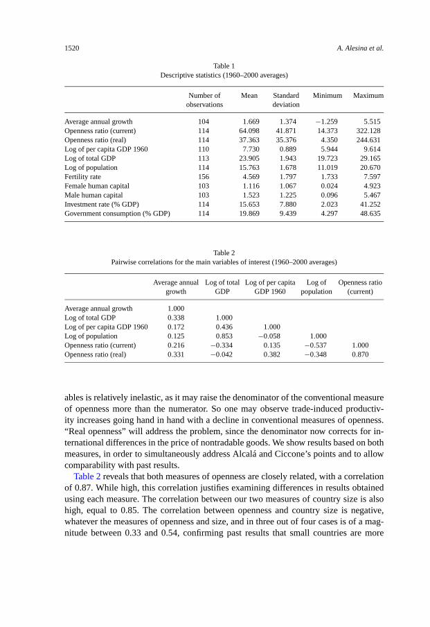
Tables 1–3 display summary statistics for our main variables of interest, averagedover the period 1960–2000. The data on openness, investment rates, growth and in-come levels, government consumption, and population come from release 6.1 of thePenn World Tables [Heston, Summers and Aten (2002)], which updates their panel ofPPP-comparable data to the year 2000. The rest of the data we use in this paper comesfrom Barro and Lee (1994, subsequently updated to 2000) or from the Central Intel-ligence Agency (2002). Country size is measured by the log of total GDP or by thelog of total population, in order to capture both economic size and demographic size.Throughout, we define trade openness in two ways: as the ratio of imports plus exportsin current prices to GDP in current prices, and as the ratio of imports plus exports in ex-change rate $U.S. to GDP in PPP $U.S. We label the first variable “nominal openness”and the second one “real openness”.
Recently, Alcalá and Ciccone (2003, 2004) have criticized the widespread use ofthe first measure, have advocated the use of the second, finding that the latter leads tomore robust effects of openness on growth. The key difference between the two mea-sure stems from the treatment of non tradable goods. Suppose that trade openness raisesproductivity, but does so more in the tradable than in the nontradable sector (a plausibleassumption). This will lead to a rise in the relative price of nontradables, and a fall inconventionally measured openness under the assumptions that the demand for nontrad-
38 Alesina, Spolaore and Wacziarg (2000) present direct evidence on the effects of market size based on levelsregressions where initial income does not appear on the right-hand side. These regressions were consistentwith the predictions of the theory presented in Section 2. We have repeated these levels regressions using thenew cross-country data that extends to 1999, with little changes in the results.
1520 A. Alesina et al.
Table 1Descriptive statistics (1960–2000 averages)
Number ofobservations
Mean Standarddeviation
Minimum Maximum
Average annual growth 104 1.669 1.374 −1.259 5.515Openness ratio (current) 114 64.098 41.871 14.373 322.128Openness ratio (real) 114 37.363 35.376 4.350 244.631Log of per capita GDP 1960 110 7.730 0.889 5.944 9.614Log of total GDP 113 23.905 1.943 19.723 29.165Log of population 114 15.763 1.678 11.019 20.670Fertility rate 156 4.569 1.797 1.733 7.597Female human capital 103 1.116 1.067 0.024 4.923Male human capital 103 1.523 1.225 0.096 5.467Investment rate (% GDP) 114 15.653 7.880 2.023 41.252Government consumption (% GDP) 114 19.869 9.439 4.297 48.635
Table 2Pairwise correlations for the main variables of interest (1960–2000 averages)
Average annualgrowth
Log of totalGDP
Log of per capitaGDP 1960
Log ofpopulation
Openness ratio(current)
Average annual growth 1.000Log of total GDP 0.338 1.000Log of per capita GDP 1960 0.172 0.436 1.000Log of population 0.125 0.853 −0.058 1.000Openness ratio (current) 0.216 −0.334 0.135 −0.537 1.000Openness ratio (real) 0.331 −0.042 0.382 −0.348 0.870
ables is relatively inelastic, as it may raise the denominator of the conventional measureof openness more than the numerator. So one may observe trade-induced productiv-ity increases going hand in hand with a decline in conventional measures of openness.“Real openness” will address the problem, since the denominator now corrects for in-ternational differences in the price of nontradable goods. We show results based on bothmeasures, in order to simultaneously address Alcalá and Ciccone’s points and to allowcomparability with past results.
Table 2 reveals that both measures of openness are closely related, with a correlationof 0.87. While high, this correlation justifies examining differences in results obtainedusing each measure. The correlation between our two measures of country size is alsohigh, equal to 0.85. The correlation between openness and country size is negative,whatever the measures of openness and size, and in three out of four cases is of a mag-nitude between 0.33 and 0.54, confirming past results that small countries are more
Ch. 23: Trade, Growth and the Size of Countries 1521
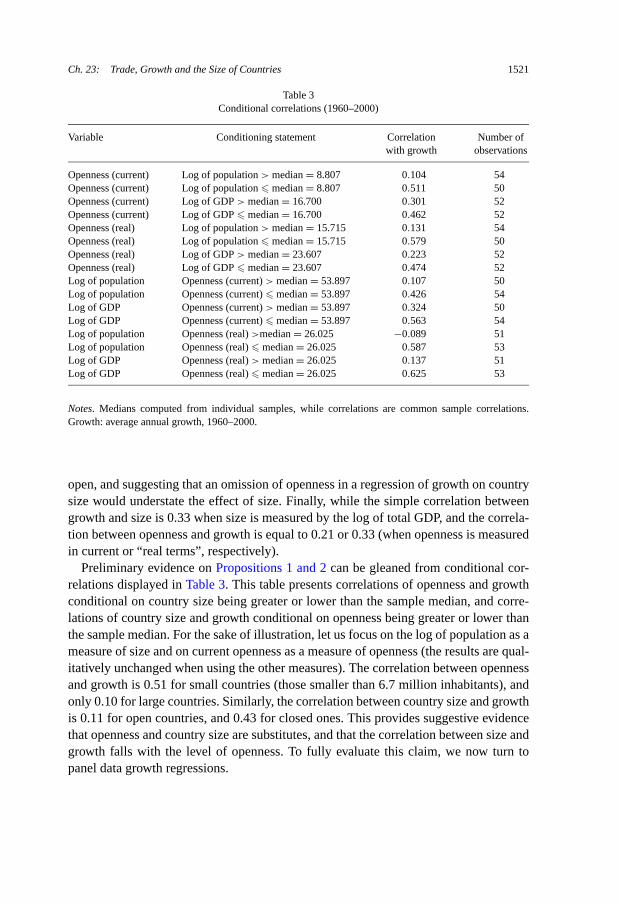
Table 3Conditional correlations (1960–2000)
Variable Conditioning statement Correlationwith growth
Number ofobservations
Openness (current) Log of population > median = 8.807 0.104 54Openness (current) Log of population � median = 8.807 0.511 50Openness (current) Log of GDP > median = 16.700 0.301 52Openness (current) Log of GDP � median = 16.700 0.462 52Openness (real) Log of population > median = 15.715 0.131 54Openness (real) Log of population � median = 15.715 0.579 50Openness (real) Log of GDP > median = 23.607 0.223 52Openness (real) Log of GDP � median = 23.607 0.474 52Log of population Openness (current) > median = 53.897 0.107 50Log of population Openness (current) � median = 53.897 0.426 54Log of GDP Openness (current) > median = 53.897 0.324 50Log of GDP Openness (current) � median = 53.897 0.563 54Log of population Openness (real) >median = 26.025 −0.089 51Log of population Openness (real) � median = 26.025 0.587 53Log of GDP Openness (real) > median = 26.025 0.137 51Log of GDP Openness (real) � median = 26.025 0.625 53
Notes. Medians computed from individual samples, while correlations are common sample correlations.Growth: average annual growth, 1960–2000.
open, and suggesting that an omission of openness in a regression of growth on countrysize would understate the effect of size. Finally, while the simple correlation betweengrowth and size is 0.33 when size is measured by the log of total GDP, and the correla-tion between openness and growth is equal to 0.21 or 0.33 (when openness is measuredin current or “real terms”, respectively).
Preliminary evidence on Propositions 1 and 2 can be gleaned from conditional cor-relations displayed in Table 3. This table presents correlations of openness and growthconditional on country size being greater or lower than the sample median, and corre-lations of country size and growth conditional on openness being greater or lower thanthe sample median. For the sake of illustration, let us focus on the log of population as ameasure of size and on current openness as a measure of openness (the results are qual-itatively unchanged when using the other measures). The correlation between opennessand growth is 0.51 for small countries (those smaller than 6.7 million inhabitants), andonly 0.10 for large countries. Similarly, the correlation between country size and growthis 0.11 for open countries, and 0.43 for closed ones. This provides suggestive evidencethat openness and country size are substitutes, and that the correlation between size andgrowth falls with the level of openness. To fully evaluate this claim, we now turn topanel data growth regressions.
1522 A. Alesina et al.
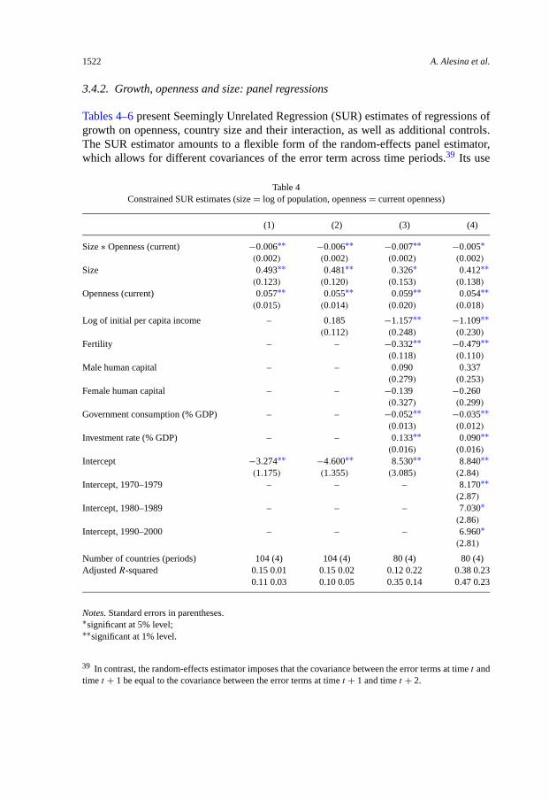
3.4.2. Growth, openness and size: panel regressions
Tables 4–6 present Seemingly Unrelated Regression (SUR) estimates of regressions ofgrowth on openness, country size and their interaction, as well as additional controls.The SUR estimator amounts to a flexible form of the random-effects panel estimator,which allows for different covariances of the error term across time periods.39 Its use
Table 4Constrained SUR estimates (size = log of population, openness = current openness)
(1) (2) (3) (4)
Size ∗ Openness (current) −0.006∗∗ −0.006∗∗ −0.007∗∗ −0.005∗(0.002) (0.002) (0.002) (0.002)
Size 0.493∗∗ 0.481∗∗ 0.326∗ 0.412∗∗(0.123) (0.120) (0.153) (0.138)
Openness (current) 0.057∗∗ 0.055∗∗ 0.059∗∗ 0.054∗∗(0.015) (0.014) (0.020) (0.018)
Log of initial per capita income – 0.185 −1.157∗∗ −1.109∗∗(0.112) (0.248) (0.230)
Fertility – – −0.332∗∗ −0.479∗∗(0.118) (0.110)
Male human capital – – 0.090 0.337(0.279) (0.253)
Female human capital – – −0.139 −0.260(0.327) (0.299)
Government consumption (% GDP) – – −0.052∗∗ −0.035∗∗(0.013) (0.012)
Investment rate (% GDP) – – 0.133∗∗ 0.090∗∗(0.016) (0.016)
Intercept −3.274∗∗ −4.600∗∗ 8.530∗∗ 8.840∗∗(1.175) (1.355) (3.085) (2.84)
Intercept, 1970–1979 – – – 8.170∗∗(2.87)
Intercept, 1980–1989 – – – 7.030∗(2.86)
Intercept, 1990–2000 – – – 6.960∗(2.81)
Number of countries (periods) 104 (4) 104 (4) 80 (4) 80 (4)Adjusted R-squared 0.15 0.01 0.15 0.02 0.12 0.22 0.38 0.23
0.11 0.03 0.10 0.05 0.35 0.14 0.47 0.23
Notes. Standard errors in parentheses.∗significant at 5% level;∗∗significant at 1% level.
39 In contrast, the random-effects estimator imposes that the covariance between the error terms at time t andtime t + 1 be equal to the covariance between the error terms at time t + 1 and time t + 2.
Ch. 23: Trade, Growth and the Size of Countries 1523
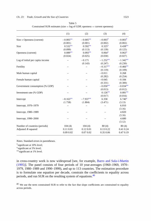
Table 5Constrained SUR estimates (size = log of GDP, openness = current openness)
(1) (2) (3) (4)
Size ∗ Openness (current) −0.005∗∗ −0.005∗∗ −0.003† −0.003†
(0.001) (0.001) (0.002) (0.002)
Size 0.532∗∗ 0.592∗∗ 0.325∗ 0.438∗∗(0.099) (0.113) (0.139) (0.125)
Openness (current) 0.089∗∗ 0.093∗∗ 0.064∗ 0.063∗(0.024) (0.025) (0.030) (0.027)
Log of initial per capita income – −0.171 −1.252∗∗ −1.342∗∗(0.143) (0.247) (0.230)
Fertility – – −0.317∗∗ −0.466∗∗(0.119) (0.109)
Male human capital – – −0.011 0.268(0.282) (0.254)
Female human capital – – −0.045 −0.184(0.331) (0.300)
Government consumption (% GDP) – – −0.050∗∗ −0.034∗∗(0.013) (0.012)
Investment rate (% GDP) – – 0.126∗∗ 0.081∗∗(0.017) (0.016)
Intercept −8.163∗∗ −7.937∗∗ 6.358 6.740∗(1.758) (1.804) (3.471) (3.13)
Intercept, 1970–1979 – – – 6.010(3.16)
Intercept, 1980–1989 – – – 4.820(3.16)
Intercept, 1990–2000 – – – 4.680(3.12)
Number of countries (periods) 104 (4) 104 (4) 80 (4) 80 (4)Adjusted R-squared 0.11 0.01 0.12 0.01 0.13 0.22 0.41 0.24
0.09 0.02 0.07 0.02 0.35 0.06 0.47 0.19
Notes. Standard errors in parentheses.†significant at 10% level;∗significant at 5% level;∗∗significant at 1% level.
in cross-country work is now widespread [see, for example, Barro and Sala-i-Martin(1995)]. The panel consists of four periods of 10 year-averages (1960–1969, 1970–1979, 1980–1989 and 1990–1999), and up to 113 countries. The estimation procedureis to formulate one equation per decade, constrain the coefficients to equality acrossperiods, and run SUR on the resulting system of equations.40
40 We use the term constrained SUR to refer to the fact that slope coefficients are constrained to equalityacross periods.
1524 A. Alesina et al.
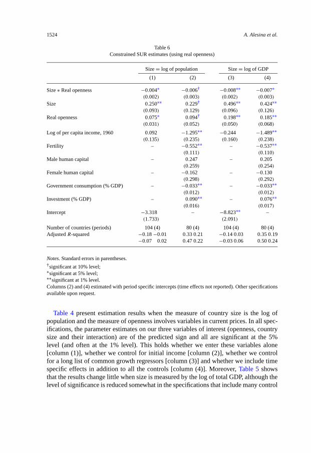
Table 6Constrained SUR estimates (using real openness)
Size = log of population Size = log of GDP
(1) (2) (3) (4)
Size ∗ Real openness −0.004∗ −0.006† −0.008∗∗ −0.007∗(0.002) (0.003) (0.002) (0.003)
Size 0.250∗∗ 0.229† 0.496∗∗ 0.424∗∗(0.093) (0.129) (0.096) (0.126)
Real openness 0.075∗ 0.094† 0.198∗∗ 0.185∗∗(0.031) (0.052) (0.050) (0.068)
Log of per capita income, 1960 0.092 −1.295∗∗ −0.244 −1.489∗∗(0.135) (0.235) (0.160) (0.238)
Fertility – −0.552∗∗ – −0.537∗∗(0.111) (0.110)
Male human capital – 0.247 – 0.205(0.259) (0.254)
Female human capital – −0.162 – −0.130(0.298) (0.292)
Government consumption (% GDP) – −0.033∗∗ – −0.033∗∗(0.012) (0.012)
Investment (% GDP) – 0.090∗∗ – 0.076∗∗(0.016) (0.017)
Intercept −3.318 – −8.823∗∗ –(1.733) (2.091)
Number of countries (periods) 104 (4) 80 (4) 104 (4) 80 (4)Adjusted R-squared −0.18 −0.01 0.33 0.21 −0.14 0.03 0.35 0.19
−0.07 0.02 0.47 0.22 −0.03 0.06 0.50 0.24
Notes. Standard errors in parentheses.†significant at 10% level;∗significant at 5% level;∗∗significant at 1% level.Columns (2) and (4) estimated with period specific intercepts (time effects not reported). Other specificationsavailable upon request.
Table 4 present estimation results when the measure of country size is the log ofpopulation and the measure of openness involves variables in current prices. In all spec-ifications, the parameter estimates on our three variables of interest (openness, countrysize and their interaction) are of the predicted sign and all are significant at the 5%level (and often at the 1% level). This holds whether we enter these variables alone[column (1)], whether we control for initial income [column (2)], whether we controlfor a long list of common growth regressors [column (3)] and whether we include timespecific effects in addition to all the controls [column (4)]. Moreover, Table 5 showsthat the results change little when size is measured by the log of total GDP, although thelevel of significance is reduced somewhat in the specifications that include many control

Ch. 23: Trade, Growth and the Size of Countries 1525
variables. Finally, Table 6 shows that using “real openness” does not modify the over-all pattern of coefficients. In fact our results are generally stronger (in the sense of theestimated coefficients being larger in magnitude) when using this measure of openness.Similar estimates in Alcalá and Ciccone (2003, written after first draft of this paper)lend further support to our results. They show how controlling for a host of additionalvariables including institutional quality does not change the nature of these results andthat the use of “real openness” leads to coefficients that are larger and more robust thanwhen using “nominal openness”.
3.5. Endogeneity of openness: 3SLS estimates
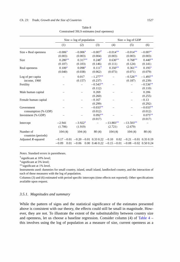
Openness, especially when defined as the volume of trade divided by GDP (howeverdeflated), may be an endogenous variable in growth regressions. As described above,in an important paper Frankel and Romer (1999) have developed a innovative instru-ment to deal with potential endogeneity bias in growth and income level regressions.We use our own set of geographic variables as well as Frankel and Romer’s instru-ment to address potential endogeneity. Our panel data IV estimator relies on a threestage least squares (3SLS) procedure. This estimator achieves consistency through in-strumentation, and efficiency through the estimation of cross-period error covarianceterms. Table 7 presents parameter estimates of our basic specification when the list ofinstruments includes geographic variables, namely dummy variables for small coun-tries, islands, small islands, landlocked countries and the interaction term between eachof these measures and country size.41 Again, the results are consistent with previousobservations, namely the pattern of coefficients suggested by theory is maintained. Inthe specification with all the controls, the statistical significance of the coefficients ofinterest is reduced slightly when real openness is used instead of current openness (Ta-ble 8), though all remain significant at the 10% level. The signs of the main coefficientsof interest are maintained and the magnitude of the openness coefficient is raised in allspecifications, confirming the results of Alcalá and Ciccone (2003, 2004).42
Finally, Table 11 shows the same results using the geography-based instrument fromFrankel and Romer (1999), as well as the interaction term between this variable andcountry size. In all specifications, the signs and basic magnitudes of the coefficientsof interest are unchanged (although when openness is entered in “real” terms, the esti-mates cease to be statistically significant at the 5% level). Spolaore and Wacziarg (2005)
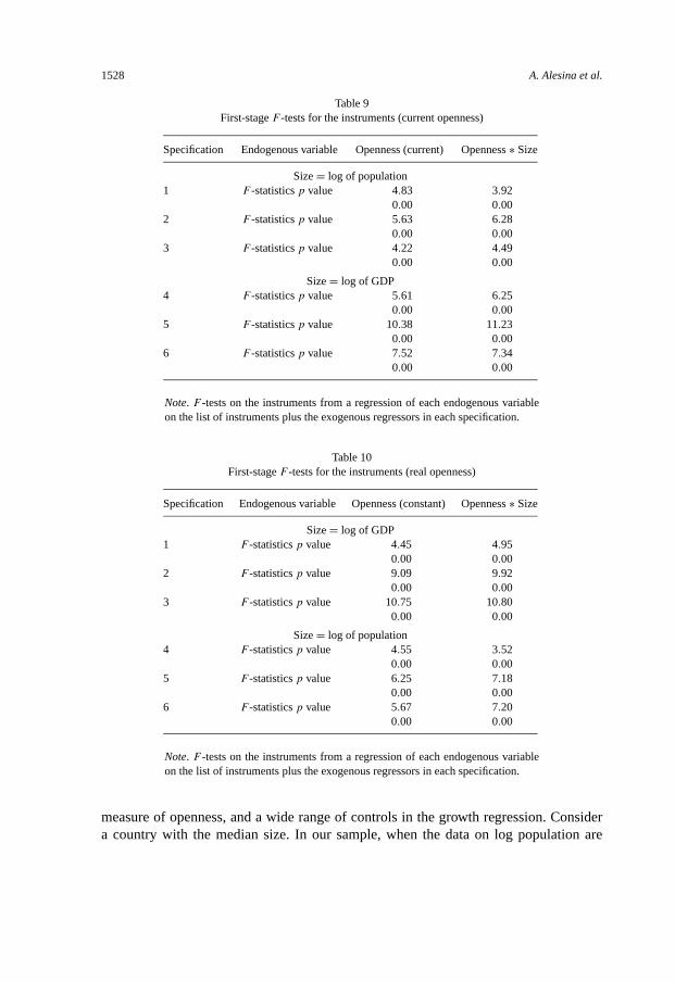
41 This is the same list of instruments as was used in Alesina, Spolaore and Wacziarg (2000). Using Hausmantests, this paper showed that this set of instruments was statistically excludable from the growth regression,and first stage F -tests suggested that they were closely related to openness and the interaction term.42 Tables 9 and 10 present F -tests for the first stage of the 3SLS procedure. They test the joint significantof the instruments in regressions of the endogenous variables (openness and its interaction with country size)on all the exogenous variables in the system. These F -tests show that our instruments are closely relatedto the variables they are instrumenting for, limiting the potential for weak instruments, especially in thespecifications with many controls.
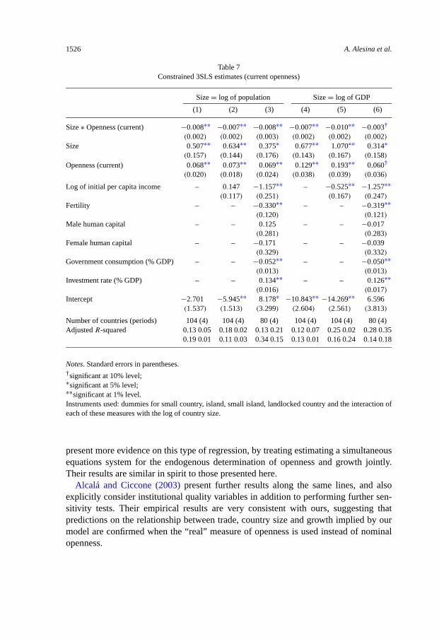
1526 A. Alesina et al.
Table 7Constrained 3SLS estimates (current openness)
Size = log of population Size = log of GDP
(1) (2) (3) (4) (5) (6)
Size ∗ Openness (current) −0.008∗∗ −0.007∗∗ −0.008∗∗ −0.007∗∗ −0.010∗∗ −0.003†
(0.002) (0.002) (0.003) (0.002) (0.002) (0.002)
Size 0.507∗∗ 0.634∗∗ 0.375∗ 0.677∗∗ 1.070∗∗ 0.314∗(0.157) (0.144) (0.176) (0.143) (0.167) (0.158)
Openness (current) 0.068∗∗ 0.073∗∗ 0.069∗∗ 0.129∗∗ 0.193∗∗ 0.060†
(0.020) (0.018) (0.024) (0.038) (0.039) (0.036)
Log of initial per capita income – 0.147 −1.157∗∗ – −0.525∗∗ −1.257∗∗(0.117) (0.251) (0.167) (0.247)
Fertility – – −0.330∗∗ – – −0.319∗∗(0.120) (0.121)
Male human capital – – 0.125 – – −0.017(0.281) (0.283)
Female human capital – – −0.171 – – −0.039(0.329) (0.332)
Government consumption (% GDP) – – −0.052∗∗ – – −0.050∗∗(0.013) (0.013)
Investment rate (% GDP) – – 0.134∗∗ – – 0.126∗∗(0.016) (0.017)
Intercept −2.701 −5.945∗∗ 8.178∗ −10.843∗∗ −14.269∗∗ 6.596(1.537) (1.513) (3.299) (2.604) (2.561) (3.813)
Number of countries (periods) 104 (4) 104 (4) 80 (4) 104 (4) 104 (4) 80 (4)Adjusted R-squared 0.13 0.05 0.18 0.02 0.13 0.21 0.12 0.07 0.25 0.02 0.28 0.35
0.19 0.01 0.11 0.03 0.34 0.15 0.13 0.01 0.16 0.24 0.14 0.18
Notes. Standard errors in parentheses.†significant at 10% level;∗significant at 5% level;∗∗significant at 1% level.Instruments used: dummies for small country, island, small island, landlocked country and the interaction ofeach of these measures with the log of country size.
present more evidence on this type of regression, by treating estimating a simultaneousequations system for the endogenous determination of openness and growth jointly.Their results are similar in spirit to those presented here.
Alcalá and Ciccone (2003) present further results along the same lines, and alsoexplicitly consider institutional quality variables in addition to performing further sen-sitivity tests. Their empirical results are very consistent with ours, suggesting thatpredictions on the relationship between trade, country size and growth implied by ourmodel are confirmed when the “real” measure of openness is used instead of nominalopenness.
Ch. 23: Trade, Growth and the Size of Countries 1527
Table 8Constrained 3SLS estimates (real openness)
Size = log of population Size = log of GDP
(1) (2) (3) (4) (5) (6)
Size ∗ Real openness −0.006∗ −0.006∗ −0.007† −0.014∗∗ −0.014∗∗ −0.007∗(0.003) (0.003) (0.004) (0.003) (0.003) (0.003)
Size 0.280∗∗ 0.317∗∗ 0.248† 0.630∗∗ 0.768∗∗ 0.440∗∗(0.107) (0.103) (0.146) (0.111) (0.124) (0.141)
Real openness 0.100∗ 0.098∗ 0.111† 0.350∗∗ 0.361∗∗ 0.195∗(0.040) (0.038) (0.062) (0.073) (0.071) (0.079)
Log of per capitaincome, 1960
– 0.017 −1.277∗∗ – −0.526∗∗ −1.493∗∗(0.157) (0.237) (0.187) (0.239)
Fertility – – −0.543∗∗ – – −0.536∗∗(0.112) (0.110)
Male human capital – – 0.269 – – 0.206(0.260) (0.255)
Female human capital – – −0.167 – – −0.13(0.299) (0.292)
Governmentconsumption (% GDP)
– – −0.033∗∗ – – −0.033∗∗(0.012) (0.012)
Investment (% GDP) – – 0.092∗∗ – – 0.075∗∗(0.017) (0.017)
Intercept −2.941 −3.922∗ – −13.883∗∗ −13.503∗∗ –(1.706) (1.919) (2.721) (2.679)
Number ofcountries (periods)
104 (4) 104 (4) 80 (4) 104 (4) 104 (4) 80 (4)
Adjusted R-squared −0.17 −0.01 −0.20 −0.01 0.33 0.22 −0.10 0.02 −0.21 −0.01 0.35 0.19−0.09 0.01 −0.06 0.00 0.46 0.22 −0.15 −0.01 −0.08 −0.02 0.50 0.24
Notes. Standard errors in parentheses.†significant at 10% level;∗significant at 5% level;∗∗significant at 1% level.Instruments used: dummies for small country, island, small island, landlocked country, and the interaction ofeach of these measures with the log of population.Columns (3) and (6) estimated with period specific intercepts (time effects not reported). Other specificationsavailable upon request.
3.5.1. Magnitudes and summary
While the pattern of signs and the statistical significance of the estimates presentedabove is consistent with our theory, the effects could still be small in magnitude. How-ever, they are not. To illustrate the extent of the substitutability between country sizeand openness, let us choose a baseline regression. Consider column (4) of Table 4 –this involves using the log of population as a measure of size, current openness as a
1528 A. Alesina et al.
Table 9First-stage F -tests for the instruments (current openness)
Specification Endogenous variable Openness (current) Openness ∗ Size
Size = log of population1 F -statistics p value 4.83 3.92
0.00 0.002 F -statistics p value 5.63 6.28
0.00 0.003 F -statistics p value 4.22 4.49
0.00 0.00
Size = log of GDP4 F -statistics p value 5.61 6.25
0.00 0.005 F -statistics p value 10.38 11.23
0.00 0.006 F -statistics p value 7.52 7.34
0.00 0.00
Note. F -tests on the instruments from a regression of each endogenous variableon the list of instruments plus the exogenous regressors in each specification.
Table 10First-stage F -tests for the instruments (real openness)
Specification Endogenous variable Openness (constant) Openness ∗ Size
Size = log of GDP1 F -statistics p value 4.45 4.95
0.00 0.002 F -statistics p value 9.09 9.92
0.00 0.003 F -statistics p value 10.75 10.80
0.00 0.00
Size = log of population4 F -statistics p value 4.55 3.52
0.00 0.005 F -statistics p value 6.25 7.18
0.00 0.006 F -statistics p value 5.67 7.20
0.00 0.00
Note. F -tests on the instruments from a regression of each endogenous variableon the list of instruments plus the exogenous regressors in each specification.
measure of openness, and a wide range of controls in the growth regression. Considera country with the median size. In our sample, when the data on log population are
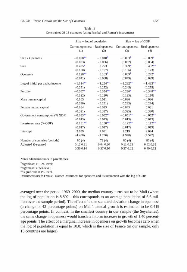
Ch. 23: Trade, Growth and the Size of Countries 1529
Table 11Constrained 3SLS estimates (using Frankel and Romer’s instrument)
Size = log of population Size = log of GDP
Current openness Real openness Current openness Real openness(1) (2) (3) (4)
Size ∗ Openness −0.008∗∗ −0.010† −0.003† −0.009∗(0.003) (0.006) (0.002) (0.004)
Size 0.435∗ 0.273 0.399∗ 0.452∗∗(0.180) (0.197) (0.166) (0.173)
Openness 0.128∗∗ 0.163† 0.089† 0.242∗(0.041) (0.088) (0.049) (0.099)
Log of initial per capita income −1.114∗∗ −1.254∗∗ −1.282∗∗ −1.433∗∗(0.251) (0.252) (0.245) (0.255)
Fertility −0.307∗ −0.354∗∗ −0.290∗ −0.348∗∗(0.122) (0.120) (0.125) (0.118)
Male human capital 0.105 −0.011 −0.036 −0.086(0.280) (0.291) (0.283) (0.284)
Female human capital −0.164 −0.023 −0.043 0.031(0.321) (0.327) (0.325) (0.320)
Government consumption (% GDP) −0.053∗∗ −0.052∗∗ −0.051∗∗ −0.052∗∗(0.013) (0.013) (0.013) (0.013)
Investment rate (% GDP) 0.131∗∗ 0.130∗∗ 0.122∗∗ 0.112∗∗(0.017) (0.017) (0.017) (0.019)
Intercept 3.959 7.991 2.219 2.694(4.408) (4.296) (4.948) (4.547)
Number of countries (periods) 80 (4) 78 (4) 80 (4) 80 (4)Adjusted R-squared 0.12 0.21 0.04 0.20 0.11 0.23 0.02 0.18
0.36 0.14 0.37 0.10 0.37 0.02 0.40 0.12
Notes. Standard errors in parentheses.†significant at 10% level;∗significant at 5% level;∗∗significant at 1% level.Instruments used: Frankel–Romer instrument for openness and its interaction with the log of GDP.
averaged over the period 1960–2000, the median country turns out to be Mali (wherethe log of population is 8.802 – this corresponds to an average population of 6.6 mil-lion over the sample period). The effect of a one standard deviation change in openness(a change of 42 percentage points) on Mali’s annual growth is estimated to be 0.419percentage points. In contrast, in the smallest country in our sample (the Seychelles),the same change in openness would translate into an increase in growth of 1.40 percent-age points. The effect of a marginal increase in openness on growth becomes zero whenthe log of population is equal to 10.8, which is the size of France (in our sample, only13 countries are larger).
1530 A. Alesina et al.
Conversely, the effect of size at the median level of openness, which is attained bySouth Korea (with a trade to GDP ratio of 54% on average between 1960 and 1999),the effect of multiplying the country’s size by 10 would be to raise annual growth by0.33 percentage points. In contrast, a relatively closed country such as Argentina (witha trade to GDP ratio of 15% on average between 1960 and 1998) would experience anincrease in growth of 0.78 percentage points from decoupling its population. The effectof size on growth attains zero when openness reaches 82.4% (in our sample, 26 countrieshad a higher level of average openness over the 1960–1999 period). Using the resultsobtained with “real” measures of openness the magnitude of our results would typicallybe even larger.
Whether one “believes” these actual magnitudes or not, the signs and statisticalsignificance of our variables of interest are very robust features of the data and inde-pendently confirmed and reinforced by Alcalá and Ciccone (2003). When evaluatingthe effects of scale on growth, it is essential to view scale as attainable either througha large domestic market, or through trade openness. Ignoring either would lead to un-derestimating scale effects in income. This section and the literature from which it isinspired has sought to bring together the research on the impact of trade on growth andthe research on the impact of economic scale on growth, and in doing so has empiricallyestablished a substitutability between openness and country size.
4. Country size and trade in history
To what extent the size of countries respond to the economic “incentives” that we dis-cussed above? Is there a sense that in the long-run the size of countries responds toeconomic forces? Our answer is yes, even though, of course, the determination of bor-ders is driven by a highly complex web of politico-economic forces. The point of thissection is simply to highlight the relationship between country size and trade in a briefhistorical excursion. We certainly we do not aim to discuss the entire history of stateformation and their size. For a more extensive discussion we refer the reader to Alesinaand Spolaore (2003), and to the voluminous literature cited therein.
4.1. The city-states
The city-states of Italy and the Low Countries of the Renaissance in Europe representa clear example of a political entity that could prosper even if very small because theywere taking advantage of world markets. Free trade was the key to prosperity of thesesmall states. A contemporary observer described Amsterdam as a place were “com-merce is absolutely free, absolutely nothing is forbidden to merchants, they have no ruleto follow but their own interest. So when an individual seems to do in his own commer-cial interest something contrary to the state the state turns a blind eye and pretends notto notice”.43 The other reason why city-states could afford to be small is that the state
43 From Braudel (1992, p. 206). Also cited in Alesina and Spolaore (2003).
Ch. 23: Trade, Growth and the Size of Countries 1531
did not provide many public goods, so that not much was lost in terms of tax burdenfrom being small. Thus, the combination of a small states who provided very few publicgoods and complete freedom of trade allowed for the city state to reach unprecedentedlevel of wealth based on trade.
4.2. The absolutist period
The emergence of centralized states from the consolidation of feudal manors was drivenby three main forces. One is technological innovations in military technology that in-creased the benefits of scale in warfare. Secondly, there was a need to enforce propertyrights and to create markets above and beyond the maritime commerce of the city-states.Finally bellicose rulers needed vast populations in order to extract levies to finance warsand luxurious courts. Territorial expansion and fiscal pressure went hand in hand andcity-states could not survive in this changed world. Italian city-states lost predominance.The Low Countries survived longer because of their role as Atlantic traders. While thesmall city-states blossomed on trade, as Wilson (1967) writes regarding France “bythe second half of the sixteenth century primitive ideas about trade had already givenrise to a corpus of legislation . . . aimed at national self-sufficiency”. Similarly, Eng-lish policy turned quite protectionist in the early seventeenth century. From the smalland open city-states with low taxation, the western world became organized in largecountries, pursuing inward looking policies. So economic predominance switched fromsmall open economies with cheap governments to large relatively closed economieswith a heavier burden of taxation to service war.
Outside the core of Europe, absolutist regimes were based on heavy taxation raisedwithout the parenthesis of city-states. This is the case, for instance of the Ottoman Em-pire, but also of India and China. The Ottoman Empire for instance, was largely basedon extracting rents from its population. In India the level of taxation was extraordinarilyhigh for that period. In the sixteenth century the estimated tax revenue of the centralgovernment was about 20% of GNP.
4.3. The birth of the modern nation-state
The nineteenth century marks the birth of the nation-state in modern forms, both in Eu-rope and North America. It also marks the beginning of industrialization and the growthtake-off, which likely transformed the relationship between country size and economicperformance, raising the importance of scale effects. The liberal philosophers of thesetimes viewed the “optimal size” of a nation-state as emerging from the trade-off be-tween homogeneity of language and culture and the benefit of economic size. In fact,following the work of Adam Smith, they were well aware that with free trade a marketeconomy can easily prosper even without a heavy central government. Nevertheless,the view was that there existed an minimum size that made an economy viable. For in-stance, certain regions, like Belgium, Ireland and Portugal were considered too small toprosper, but free trade was regarded as a way of allowing even relatively small countries
1532 A. Alesina et al.
to prosper. Giuseppe Mazzini, an architect of the Italian unification, suggested that theoptimal number of states in Europe was 12. His argument was precisely based on theconsideration of a trade-off between the economically viable size of country and na-tionalistic aspiration of various groups. A famous political economy treaty of the timeargues that it was “ridiculous” that Belgium and Portugal should be independent be-cause there economies were too small to be economically viable.44
The unification of Germany can in fact be viewed along similar lines. The Germannation-state started as a customs union (the Zollverein) which was viewed as necessaryto create a sufficiently large market. As Merriman (1996, p. 629) notes, before the cus-toms union “German merchants and manufacturers began to object to the discouragingcomplexity of custom tariffs that created a series of costly hurdles . . . many business-men demanded an end to these unnatural impediments faced by neither of their Frenchor British rivals”. Clearly market size was a critical determinant of the birth of Ger-many. The external threat of a war with France was a second one, as emphasized byRiker (1964). The establishment of a common market free of trade barriers was alsoone of the motivating factor behind the creation of the United States.
4.4. The colonial empires
In the period between 1848 and early 1870’s the share of international trade inGDP quadrupled in Europe.45 From 1870 to the First World War trade grew muchmore slowly despite a drastic reduction of transportation costs, as documented inEstevadeordal, Frantz and Taylor (2003). In fact the extent of the reduction of tradeamongst European powers in the half-century between 1870 and 1915 is a matter ofdispute amongst historians. Bairoch (1989) has probably the most sanguine view onone side of the argument when he writes that the introduction of new large tariff byGermany in 1879 marks the “death” of free trade. While many historians may find thisview a bit extreme, it is fairly noncontroversial that without the sharp reduction in trad-ing costs international trade would have probably greatly suffered in this period, whichwas certainly associated with an increase in protectionism.
The last two decades of the nineteenth century witnessed the expansion of European(and North American) powers over much of the “less developed” world. One motivationof this expansionary policy was certainly the opening of new markets. As reported byHobsbawm (1987, p. 67), in 1897 the British Prime Minister told the French ambassadorto Britain that “if you [the French] were not such persistent protectionists, you wouldnot find us so keen to annex new territories”. Needless to say, the British were just asprotectionist as the French and the British navy was heavily used to protect trade routes.Similar considerations apply to the expansionary acquisitions of the United States in thelate nineteenth and early twentieth centuries, namely Alaska, Hawaii, Samoa, Cuba andthe Philippines. At the same time, in response to European protectionism, the UnitedStates also turned protectionist in this period.
44 See Hobsbawm (1987).45 See Estevadeordal, Frantz and Taylor (2003) for a more detailed discussion.
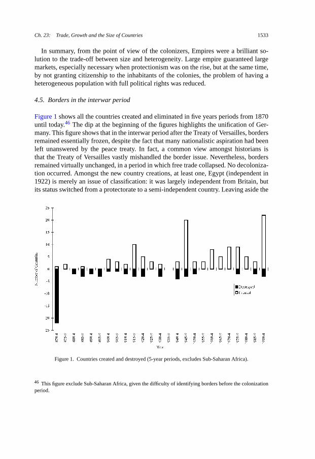
Ch. 23: Trade, Growth and the Size of Countries 1533
In summary, from the point of view of the colonizers, Empires were a brilliant so-lution to the trade-off between size and heterogeneity. Large empire guaranteed largemarkets, especially necessary when protectionism was on the rise, but at the same time,by not granting citizenship to the inhabitants of the colonies, the problem of having aheterogeneous population with full political rights was reduced.
4.5. Borders in the interwar period
Figure 1 shows all the countries created and eliminated in five years periods from 1870until today.46 The dip at the beginning of the figures highlights the unification of Ger-many. This figure shows that in the interwar period after the Treaty of Versailles, bordersremained essentially frozen, despite the fact that many nationalistic aspiration had beenleft unanswered by the peace treaty. In fact, a common view amongst historians isthat the Treaty of Versailles vastly mishandled the border issue. Nevertheless, bordersremained virtually unchanged, in a period in which free trade collapsed. No decoloniza-tion occurred. Amongst the new country creations, at least one, Egypt (independent in1922) is merely an issue of classification: it was largely independent from Britain, butits status switched from a protectorate to a semi-independent country. Leaving aside the
Figure 1. Countries created and destroyed (5-year periods, excludes Sub-Saharan Africa).
46 This figure exclude Sub-Saharan Africa, given the difficulty of identifying borders before the colonizationperiod.
1534 A. Alesina et al.
Vatican City, the only other countries created between 1920 and the Second World Warwere Ireland (1921), Mongolia (1921), Iraq (1932), and Saudi Arabia (1932).
The interwar period was characterized by a collapse of free trade, the emergence ofdictatorships, and by a belligerent state of international relationships. The Great De-pression completed the gloomy picture and precipitated the rise of protectionism. Theseare all factors that, according to our analysis, should not be associated with the creationof new countries, in fulfillment of nationalistic aspirations. In addition, these elements(lack of democracy, international conflicts, protectionism) would make colonial powershold on to their empires and repress independent movements. In fact, all the colonialpowers were adamant in refusing self-determination of colonies during this period. Thiscombinations of events, protectionism and maintenance of large countries and empire,stands in sharp contrast with what happened in the aftermath of the Second World War.
4.6. Borders in the post–Second World War period
In the fifty years that followed the Second World War, the number of independent coun-tries increased dramatically. There were 74 countries in 1948, 89 in 1950, and 193in 2001. The world now comprises a large number of relatively small countries: in 1995,87 of the countries in the world had a population of less than 5 million, 58 had a pop-ulation of less than 2.5 million, and 35 less than 500 thousands. In the same 50 years,the share of international trade in world GDP increased dramatically. The volume ofimports and exports in a sample of about 60 countries has risen by about 40 percent.
We should stress that the increase in international trade in the last half-century, asdocumented in Figure 2, is not the simple result of an accounting illusion. In fact, if
Figure 2. Trade openness and the number of countries.
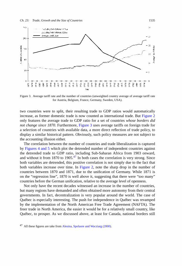
Ch. 23: Trade, Growth and the Size of Countries 1535
Figure 3. Average tariff rate and the number of countries (unweighted country average of average tariff ratefor Austria, Belgium, France, Germany, Sweden, USA).
two countries were to split, their resulting trade to GDP ratios would automaticallyincrease, as former domestic trade is now counted as international trade. But Figure 2only features the average trade to GDP ratio for a set of countries whose borders didnot change since 1870. Furthermore, Figure 3 uses average tariffs on foreign trade fora selection of countries with available data, a more direct reflection of trade policy, todisplay a similar historical pattern. Obviously, such policy measures are not subject tothe accounting illusion either.
The correlation between the number of countries and trade liberalization is capturedby Figures 4 and 5 which plot the detrended number of independent countries againstthe detrended trade to GDP ratio, including Sub-Saharan Africa from 1903 onward,and without it from 1870 to 1905.47 In both cases the correlation is very strong. Sinceboth variables are detrended, this positive correlation is not simply due to the fact thatboth variables increase over time. In Figure 2, note the sharp drop in the number ofcountries between 1870 and 1871, due to the unification of Germany. While 1871 ison the “regression line”, 1870 is well above it, suggesting that there were “too many”countries before the German unification, relative to the average level of openness.
Not only have the recent decades witnessed an increase in the number of countries,but many regions have demanded and often obtained more autonomy from their centralgovernments. In fact, decentralization is very popular around the world. The case ofQuébec is especially interesting. The push for independence in Québec was revampedby the implementation of the North American Free Trade Agreement (NAFTA). Thefreer trade in North America, the easier it would be for a relatively small country, likeQuébec, to prosper. As we discussed above, at least for Canada, national borders still
47 All these figures are take from Alesina, Spolaore and Wacziarg (2000).
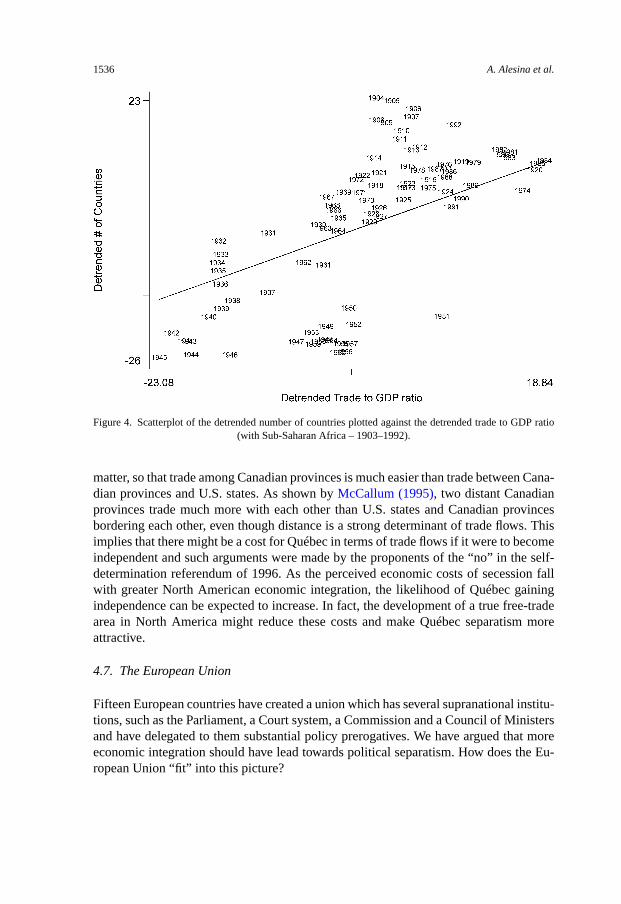
1536 A. Alesina et al.
Figure 4. Scatterplot of the detrended number of countries plotted against the detrended trade to GDP ratio(with Sub-Saharan Africa – 1903–1992).
matter, so that trade among Canadian provinces is much easier than trade between Cana-dian provinces and U.S. states. As shown by McCallum (1995), two distant Canadianprovinces trade much more with each other than U.S. states and Canadian provincesbordering each other, even though distance is a strong determinant of trade flows. Thisimplies that there might be a cost for Québec in terms of trade flows if it were to becomeindependent and such arguments were made by the proponents of the “no” in the self-determination referendum of 1996. As the perceived economic costs of secession fallwith greater North American economic integration, the likelihood of Québec gainingindependence can be expected to increase. In fact, the development of a true free-tradearea in North America might reduce these costs and make Québec separatism moreattractive.
4.7. The European Union
Fifteen European countries have created a union which has several supranational institu-tions, such as the Parliament, a Court system, a Commission and a Council of Ministersand have delegated to them substantial policy prerogatives. We have argued that moreeconomic integration should have lead towards political separatism. How does the Eu-ropean Union “fit” into this picture?
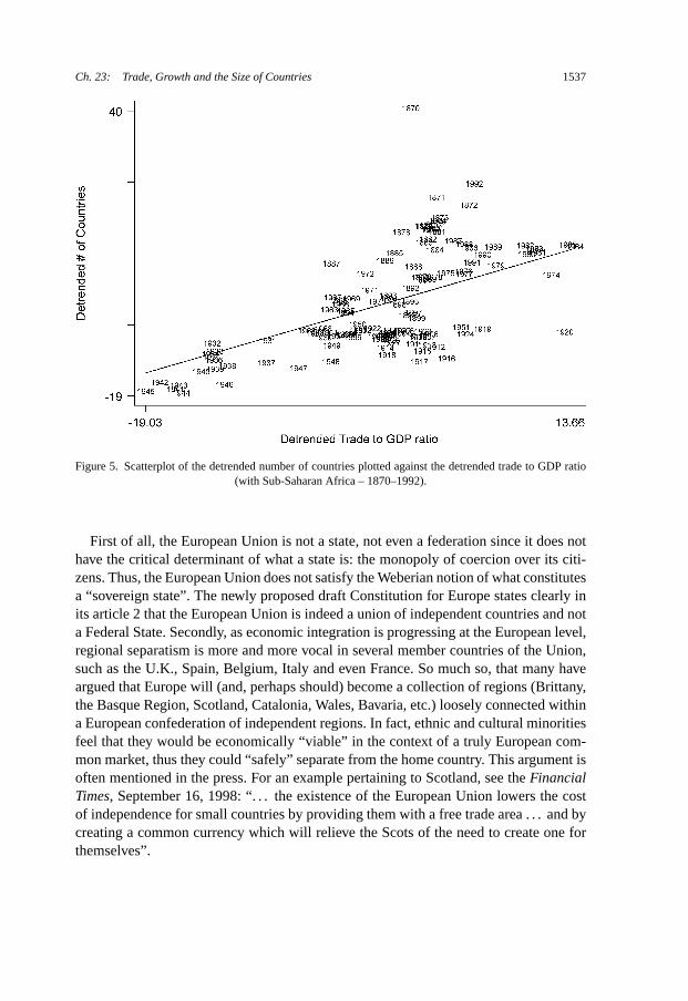
Ch. 23: Trade, Growth and the Size of Countries 1537
Figure 5. Scatterplot of the detrended number of countries plotted against the detrended trade to GDP ratio(with Sub-Saharan Africa – 1870–1992).
First of all, the European Union is not a state, not even a federation since it does nothave the critical determinant of what a state is: the monopoly of coercion over its citi-zens. Thus, the European Union does not satisfy the Weberian notion of what constitutesa “sovereign state”. The newly proposed draft Constitution for Europe states clearly inits article 2 that the European Union is indeed a union of independent countries and nota Federal State. Secondly, as economic integration is progressing at the European level,regional separatism is more and more vocal in several member countries of the Union,such as the U.K., Spain, Belgium, Italy and even France. So much so, that many haveargued that Europe will (and, perhaps should) become a collection of regions (Brittany,the Basque Region, Scotland, Catalonia, Wales, Bavaria, etc.) loosely connected withina European confederation of independent regions. In fact, ethnic and cultural minoritiesfeel that they would be economically “viable” in the context of a truly European com-mon market, thus they could “safely” separate from the home country. This argument isoften mentioned in the press. For an example pertaining to Scotland, see the FinancialTimes, September 16, 1998: “. . . the existence of the European Union lowers the costof independence for small countries by providing them with a free trade area . . . and bycreating a common currency which will relieve the Scots of the need to create one forthemselves”.
1538 A. Alesina et al.
One way of thinking about the EU is as a supranational union of countries that havemerged certain functions needed to guarantee the functioning of a common market andtake advantage of economies of scale. Whether or not the attribution of responsibilitiesand policy prerogatives between the EU and the national government is appropriate ornot is an intricate subject which is beyond the scope of this paper.48
5. Conclusion
This paper has argued that size matters for economic performance and that country sizeis endogenous and depends on economic factors such as free trade, public goods pro-vision and preference heterogeneity. We have reviewed and extended a recent literaturethat has discussed country formation and secession in the context of the theory of eco-nomic growth. The econometric and historical evidence is broadly consistent with theimplications of these models
Much remains to be done. On the theoretical side, we have shown how scale effectscould be derived in a simple neoclassical growth model, without appealing to increasingreturns technologies, endogenous R&D or human capital spillovers, but simply by ap-pealing to the existence of a border effect driven by trading frictions. However, whetherthe scale effects that we observe in the data come from the border effect, technology orspillovers remains to be investigated.
The models that we discussed are based on the assumption that heterogeneity withina country has negative effects on average utility. However, heterogeneity may also bringabout some benefits. In fact, the gains from trade in our model do stem from a kind ofheterogeneity – the production of different intermediate goods by different regions –and this is why a larger country, for given barriers to trade, brings net economic gainsthrough the trade channel. By “heterogeneity” costs here we mean the specific costsassociated with disagreements over the basic characteristics of a government (includingpolicies about official languages, religion, etc.). A richer discussion of the pros and consof heterogeneity is certainly called for.
On the empirical side, debates are still raging. Even the literature on the effect oftrade on economic performance is now subject to debates on the nature and extent ofthis effect. The literature on the effect of country size is even more contentious. Yet theexistence of both of these effects is important to the argument that we proposed aboutthe role of trade openness in the endogenous determination of country size. We haveshown that a simultaneous consideration of an economy’s openness and of its size ledto estimating strong effects of both size and openness on growth in a sample of countriessince 1960.
Finally, in a broad historical sweep, we have suggested that the types of trade-offsidentified by our framework have been at play at various stages in modern history.
48 For a discussion of this point, see Alesina and Wacziarg (1999).
Ch. 23: Trade, Growth and the Size of Countries 1539
In a way, current developments provide an ideal setting for observers of country cre-ation. Since the Second World War, increasing globalization has threatened nation-states“from above”, while rising regionalism and decentralizing forces have threatened them“from below”. The construction of the European Union epitomizes this tension, as afundamental redrawing of the distribution of political prerogatives is being orchestrated.Powers are being transferred down through decentralization, and up through the Euro-pean construction. It is likely that if globalization proceeds apace, so will regionalism.If the backlash against globalization succeeds, however, large centralized nation-statescould initiate a comeback.
Acknowledgements
We are grateful to the NSF for financial support with a grant through the NBER. Wealso thank Jessica Seddon Wallack for excellent research assistance. We thank PhilippeAghion, Francisco Alcalá, Michele Boldrin, Antonio Ciccone, Yannis Ioannides andseminar and conference participants at the University of Modena, Harvard University,the European University Institute, the University of Rochester, and New York Universityfor useful comments. All remaining errors are ours.
References
Ades, A., Glaeser, E. (1999). “Evidence on growth, increasing returns and the extent of the market”. QuarterlyJournal of Economics 114 (3), 1025–1045.
Aghion, P., Howitt, P. (1992). “A model of growth through creative destruction”. Econometrica 60, 323–351.Aghion, P., Howitt, P. (1998). “Market structure and the growth process”. Review of Economic Dynamics 1,
276–305.Aghion, P., Bloom, N., Blundell, R., Griffith, R., Howitt, P. (2002). “Competition and innovation: An inverted
U relationship”. Working Paper, September. Harvard University.Alcalá, F., Ciccone, A. (2003). “Trade, the extent of the market and economic growth 1960–1996”. Unpub-
lished Manuscript. Universitat Pompeu Fabra.Alcalá, F., Ciccone, A. (2004). “Trade and productivity”. Quarterly Journal of Economics 119 (2), 613–646.Alesina, A., Baqir, R., Easterly, W. (1999). “Public goods and ethnic divisions”. Quarterly Journal of Eco-
nomics 114 (4), 1243–1284.Alesina, A., Baqir, R., Hoxby, C. (2004). “Political jurisdictions in heterogeneous communities”. Journal of
Political Economy 112 (2), 348–396.Alesina, A., Barro, R., Tenreyro, S. (2002). “Optimal currency areas”. In: Gertler, M., Rogoff, K. (Eds.),
NBER Macroeconomic Annual, vol. 17. MIT Press, Cambridge, MA, pp. 301–345.Alesina, A., Devleeschauwer, A., Easterly, W., Kurlat, S., Wacziarg, R. (2003). “Fractionalization”. Journal
of Economic Growth 8 (2), 155–194.Alesina, A., La Ferrara, E. (2000). “Participation in heterogeneous communities”. Quarterly Journal of Eco-
nomics 115 (3), 847–904.Alesina, A., La Ferrara, E. (2002). “Who trusts others?”. Journal of Public Economics 85 (August), 207–234.Alesina, A., Spolaore, E. (1997). “On the number and size of nations”. Quarterly Journal of Economics 112
(4), 1027–1056.Alesina, A., Spolaore, E. (2003). The Size of Nations. MIT Press, Cambridge, MA.
1540 A. Alesina et al.
Alesina, A., Spolaore, E., Wacziarg, R. (2000). “Economic integration and political disintegration”. AmericanEconomic Review 90 (5), 1276–1296.
Alesina, A., Wacziarg, R. (1998). “Openness, country size and the government”. Journal of Public Eco-nomics 69 (3), 305–321.
Alesina, A., Wacziarg, R. (1999). “Is Europe going too far?”. Carnegie–Rochester Conference Series onPublic Policy 51 (1), 1–42.
Backus, D., Kehoe, P., Kehoe, T. (1992). “In search of scale effects in trade and growth”. Journal of EconomicTheory 58 (2), 377–409.
Bairoch, P. (1989). “European trade policy, 1815–1914”. In: Mathias, P., Pollard, S. (Eds.), The CambridgeEconomic History of Europe, vol. 8. Cambridge University Press, Cambridge, pp. 1–160.
Bardhan, P. (2002). “Decentralization of governance and development”. Journal of Economic Perspectives 16(4), 185–205.
Barro, R.J., Lee, J.-W. (1994). “Data set for a panel of 138 countries”, available at http://www.nber.org/data/ .Barro, R.J., Sala-i-Martin, X. (1995). Economic Growth. McGraw Hill, New York.Ben-David, D. (1993). “Equalizing exchange: Trade liberalization and income convergence”. Quarterly Jour-
nal of Economics 108 (3), 653–679.Bolton, P., Roland, G. (1997). “The breakups of nations: A political economy analysis”. Quarterly Journal of
Economics (4), 1057–1089.Braudel, F. (1992). The Perspective of the World: Civilization and Capitalism 15th–18th Century, vol. 3.
University of California Press, Berkeley.Casella, A., Feinstein, J.S. (2002). “Public goods in trade: On the formation of markets and political jurisdic-
tions”. International Economic Review 43 (2), 437–462.Central Intelligence Agency (2002). CIA World Factbook. Brassey’s Inc., Dulles, VA.De Figueiredo, R., Weingast, B. (2002), “Self-enforcing federalism”. Working Paper, March. Stanford Uni-
versity.Dollar, D. (1992). “Outward-oriented developing economies really do grow more rapidly: Evidence from 95
LDCs, 1976–85”. Economic Development and Cultural Change 40 (3), 523–544.Easterly, W., Levine, R. (1997). “Africa’s growth tragedy: Policies and ethnic divisions”. Quarterly Journal of
Economics 111 (4), 1203–1250.Edwards, S. (1993). “Openness, trade liberalization and growth in developing countries”. Journal of Economic
Literature 31 (September), 1358–1393.Edwards, S. (1998). “Openness, productivity and growth: What do we really know?”. Economic Journal 108
(447), 383–398.Estevadeordal, A., Frantz, B., Taylor, A.M. (2003). “The rise and fall of world trade, 1870–1939”. Quarterly
Journal of Economics 118 (2), 359–407.Findlay, R. (1996). “Towards a model of territorial expansion and the limits of empires”. In: Garfinkel, M.,
Skaperdas, S. (Eds.), The Political Economy of Conflict and Appropriation. Cambridge University Press,Cambridge, U.K.
Frankel, J.A., Romer, D. (1999). “Does trade cause growth?”. American Economic Review 89 (3), 379–399.Friedman, D. (1977). “A theory of the size and shape of nations”. Journal of Political Economy 85 (1), 59–77.Garner, P. (2001). “The role of rival nation-states in long-run growth”. Working Paper. Brown University.Grossman, G., Helpman, E. (1991). Innovation and Growth in the Global Economy. MIT Press, Cambridge,
MA.Ha, J., Howitt, P. (2004). “Accounting for trends in productivity and R&D: A Schumpeterian critique of
semi-endogenous growth theory”. Working Paper. Brown University.Harrison, A., Hanson, G. (1999). “Who gains from trade reforms? Some remaining puzzles”. Journal of
Development Economics 48, 419–447.Helliwell, J. (1998). How Much Do National Borders Matter? Brookings Institution Press, Washington, DC.Herbst, J. (2000). States and Power in Africa. Princeton University Press, Princeton, NJ.Heston, A., Summers, R., Aten, B. (2002). “Penn World Table, version 6.1”. Center for International Com-
parisons at the University of Pennsylvania (CICUP). October.
Ch. 23: Trade, Growth and the Size of Countries 1541
Hobsbawm, E. (1987). The Age of Empire. Vintage Books, New York, NY.Howitt, P. (1999). “Steady endogenous growth with population and R&D inputs growing”. Journal of Political
Economy 107 (4), 715–730.Jones, C. (1999). “Growth: With or without scale effects?”. American Economic Review Papers and Proceed-
ings 89 (May), 139–144.Jones, C. (1995a). “R&D-based models of economic growth”. Journal of Political Economy 103 (August),
759–784.Jones, C. (1995b). “Time series tests of endogenous growth models”. Quarterly Journal of Economics 110
(2), 495–525.La Porta, R., Lopez de Silanes, F., Shleifer, A., Vishny, R. (1999). “The quality of government”. Journal of
Law, Economics and Organization 15 (1), 222–279.Lucas, R.E. (1988). “On the mechanics of economic development”. Journal of Monetary Economics 22, 3–42.McCallum, J. (1995). “National borders matter: Canada–US regional trade patterns”. American Economic
Review 85 (3), 615–623.Merriman, J.W. (1996). A History of Modern Europe: From the Renaissance to the Present. W.W. Norton &
Co., New York.Murphy, K., Shleifer, A., Vishny, R. (1989). “Industrialization and the big push”. Journal of Political Econ-
omy 87 (5), 1003–1026.Oates, W.E. (1999). “An essay on fiscal federalism”. Journal of Economic Literature 37 (September), 1120–
1149.Obstfeld, M., Rogoff, K. (2000). “The six major puzzles in international finance: Is there a common cause?”.
In: Bernanke, B.S., Rogoff, K. (Eds.), NBER Macroeconomics Annual, vol. 15. MIT Press, CambridgeMA, pp. 339–390.
Portes, R., Rey, H. (2000). “The determinants of cross-border equity flows”. NBER Working Paper 7336,September.
Pritchett, L. (1996). “Measuring outward orientation: Can it be done?”. Journal of Development Economics 49(2), 307–335.
Riker, W.H. (1964). Federalism: Origins, Operation, Significance. Little Brown, Boston.Rodrik, D., Rodríguez, F. (2000). “Trade policy and economic growth: A skeptics guide to the cross-national
evidence”. In: Bernanke, B., Rogoff, K. (Eds.), NBER Macroeconomics Annual, vol. 15. MIT Press,Cambridge, MA, pp. 261–325.
Rodrik, D., Subramanian, A., Trebbi, F. (2004). “Institutions rule: The primary of institutions over geographyand integration in economic development”. Journal of Economic Growth 9 (2), 131–165.
Romer, P. (1986). “Increasing returns and long run growth”. Journal of Political Economy 94, 1002–1037.Romer, P. (1990). “Endogenous technological change”. Journal of Political Economy 98 (5), S71–S102.Rose, A. (2000). “One money, one market: The effect of common currencies on trade”. Economic Pol-
icy 15 (30).Sachs, J., Warner, A. (1995). “Economic reform and the process of global integration”. Brookings Papers on
Economic Activity 1, 1–118.Smith, A. (1986). An Inquiry into the Nature and Causes of the Wealth of Nations. Penguin Books, Har-
mondsworth, U.K. (first published 1776).Spolaore, E. (1995). “Economic integration, political borders and productivity”. Prepared for the CEPR–Sapir
conference on “Regional Integration and Economic Growth”. Tel Aviv University, December.Spolaore, E. (2002). “Conflict, trade and the size of countries”. Working Paper. Brown University.Spolaore, E. (2005). “The political economy of national borders”. In: Weingast, B.R., Wittman, D. (Eds.),
The Oxford Handbook of Political Economy. Oxford University Press, Oxford, in preparation.Spolaore, E., Wacziarg, R. (2005). “Borders and growth”. Journal of Economic Growth 10 (4), in press.Wacziarg, R. (2001). “Measuring the dynamic gains from trade”. World Bank Economic Review 15 (3), 393–
429.Wacziarg, R., Welch, K.H. (2003). “Trade liberalization and growth: New evidence”. NBER Working Paper
10152, December.

1542 A. Alesina et al.
Wilson, C.H. (1967). “Trade, society and the state”. In: Rich, E.E., Wilson, C.H. (Eds.), The CambridgeEconomic History of Europe from the Decline of the Roman Empire, vol. 4. Cambridge University Press,Cambridge, pp. 487–575.
Young, A. (1998). “Growth without scale effects”. Journal of Political Economy 106 (February), 41–63.