Country Size, International Trade, and Aggregate Fluctuations

in Granular Economies∗

Julian di GiovanniInternational Monetary Fund

Andrei A. LevchenkoUniversity of Michigan

and NBER

October 1, 2012

Abstract

This paper proposes a new mechanism by which country size and international tradeaffect macroeconomic volatility. We study a multi-country, multi-sector model withheterogeneous firms that are subject to idiosyncratic firm-specific shocks. When thedistribution of firm sizes follows a power law with an exponent close to −1, the idiosyn-cratic shocks to large firms have an impact on aggregate output volatility. We explorethe quantitative properties of the model calibrated to data for the 50 largest economiesin the world. Smaller countries have fewer firms, and thus higher volatility. The modelperforms well in matching this pattern both qualitatively and quantitatively: the rateat which macroeconomic volatility decreases in country size in the model is very close towhat is found in the data. Opening to trade increases the importance of large firms tothe economy, thus raising macroeconomic volatility. Our simulation exercise shows thatthe contribution of trade to aggregate fluctuations depends strongly on country size:in the largest economies in the world, such as the U.S. or Japan, international tradeincreases volatility by only 1.5-3.5%. By contrast, trade increases aggregate volatilityby some 15-20% in a small open economy, such as Denmark or Romania.

JEL Classifications: F12, F15, F41

Keywords: Macroeconomic Volatility, Firm-Level Idiosyncratic Shocks, Large Firms,International Trade

∗We are grateful to the editor (Sam Kortum), two anonymous referees, Michael Alexeev, Stijn Claessens,Aaron Flaaen, Fabio Ghironi, Gordon Hanson, Chris House, Marc Melitz, Andy Rose, Matthew Shapiro,Linda Tesar, and workshop participants at various institutions for helpful suggestions, and to EdithLaget, Lin Ma, and Ryan Monarch for expert research assistance. Levchenko thanks the National Sci-ence Foundation for financial support under grant SES-0921971. The views expressed in this paperare those of the authors and should not be attributed to the International Monetary Fund, its Ex-ecutive Board, or its management. E-mail (URL): JdiGiovanni@imf.org (http://julian.digiovanni.ca),alev@umich.edu (http://www.alevchenko.com). The Supplementary Web Appendix to this paper is availableat http://alevchenko.com/diGiovanni Levchenko granular web appendix.pdf.

1 Introduction

Output volatility varies substantially across economies: over the past 35 years, the standard

deviation of annual real per capita GDP growth has been 2.5 times higher in non-OECD

countries compared to the OECD countries. Understanding the sources of these differences

is important, as aggregate volatility itself has an impact on a wide variety of economic

outcomes.1

This paper investigates the role of large firms in explaining cross-country differences in

aggregate volatility. We show that the impact of shocks to large firms on aggregate volatility

can help account for two robust empirical regularities: (i) smaller countries are more volatile;

and (ii) more open countries are more volatile. The key ingredient of our study is that the

distribution of firm size is very fat-tailed – the typical economy is dominated by a few

very large firms (Axtell, 2001). In a recent contribution, Gabaix (2011) demonstrates that

under these conditions idiosyncratic shocks to individual firms do not cancel out and can

instead generate aggregate fluctuations (see also Delli Gatti et al., 2005). Gabaix (2011)

provides both statistical and anecdotal evidence that even in the largest and most diversified

economy in the world – the United States – shocks to the biggest firms can appreciably affect

macroeconomic fluctuations. The economy is “granular” rather than smooth.

We develop a theoretical and quantitative framework to study the consequences of this

phenomenon in a large cross section of countries. The analysis is based on the canonical

multi-country model with heterogeneous firms in the spirit of Melitz (2003) and Eaton et al.

(2011), implemented on the 50 largest economies in the world. In order to study the impact

of large firms on aggregate fluctuations, the equilibrium total number of firms is determined

endogenously in the model, and the parameters are calibrated to match the observed firm

size distribution. The solution procedure targets the key aggregate country characteristics

– GDPs and average trade volumes – and successfully reproduces a number of non-targeted

features of the micro data, such as the share firms that export and the relative size of the

largest firms across countries.

Our main results can be summarized as follows. First, the model endogenously generates

a negative relationship between country size and aggregate volatility. The reason is that

smaller countries will have a smaller equilibrium number of firms (as implied by many

models since at least Krugman, 1980), and thus shocks to the largest firms will matter more

1Numerous studies identify its effects on long-run growth (Ramey and Ramey, 1995), welfare (Pallageand Robe, 2003; Barlevy, 2004), as well as inequality and poverty (Gavin and Hausmann, 1998; Laursen andMahajan, 2005).

1

for aggregate volatility. In effect, smaller economies are less diversified, when diversification

is measured at the firm level. The model matches this relationship not only qualitatively,

but also quantitatively: the rate at which volatility decreases in country size in the model

is very similar to what is observed in the data. Both in the model and in the data, a

typical country that accounts for 0.5% of world GDP (such as Poland or South Africa) has

aggregate volatility that is 2 times higher than the largest economy in the world – the U.S..

Second, trade openness increases volatility by making the economy more granular. When

a country opens to trade, only the largest and most productive firms export, while smaller

firms shrink or disappear (Melitz, 2003). This effect implies that after opening, the biggest

firms become even larger relative to the size of the economy, thus contributing more to

aggregate output fluctuations. In the counterfactual exercise, we compute what aggregate

volatility would be for each country in autarky, and compare it to the volatility under

the current trade costs. It turns out that at the levels of trade openness observed today,

international trade increases volatility relative to autarky in every country. The importance

of trade for aggregate volatility varies greatly depending on country characteristics. In the

largest economies like Japan or the U.S., aggregate volatility is only 1.5-3.5% higher than

it would have been in complete autarky. In small, remote economies such as South Africa

or New Zealand, trade raises volatility by about 10% compared to autarky. Finally, in

small, highly integrated economies such as Denmark or Romania, international trade raises

aggregate volatility by some 15-20%.

The theoretical link between country size, trade openness, and volatility we explore in

this paper has not previously been proposed. Head (1995) and Crucini (1997) examine the

relationship between country size and volatility in a 2-country international real business

cycle (IRBC) model. In those papers, the smaller country has higher volatility because the

world interest rate is less sensitive to shocks occurring in that country. Thus, following a

positive shock it can expand investment without much of an impact on interest rates.2 Our

explanation for the size-volatility relationship is qualitatively different, and relies instead

on the notion that smaller countries have fewer firms. When it comes to the relationship

between trade openness and volatility, existing explanations have focused on the propagation

2The Supplementary Web Appendix implements the canonical IRBC model of Backus et al. (1995), andexamines the relationship between country size and volatility, and between trade openness and volatility,in that model. It turns out that while the calibrated IRBC model can produce higher volatility in smallercountries, the relationship between country size and volatility in that model is two orders of magnitudeflatter than what is observed in the data. The relationship between trade openness and volatility in theIRBC model is ambiguous, its sign depending crucially on the elasticity of substitution between domesticand foreign goods.

2

of global demand or supply shocks (Newbery and Stiglitz, 1984; Kraay and Ventura, 2007).

We show that trade can increase volatility even if the nature of shocks affecting the firms

is unchanged upon opening. Finally, the mechanism in our model resembles the traditional

arguments that smaller countries, and more open countries, will have a less diversified

sectoral production structure, and thus exhibit higher volatility (see Katzenstein, 1985;

OECD, 2006; Blattman et al., 2007, among many others). Our analysis shows that this

argument applies to individual firms as well as sectors, and makes this point quantitatively

precise by calibrating the model to the observed firm size distribution.

Our work is also related to the empirical literature that studies macroeconomic volatility

using disaggregated data. Koren and Tenreyro (2007) explore the importance of sector-

specific shocks in explaining the relationship between a country’s level of development and

its aggregate volatility, while di Giovanni and Levchenko (2009, 2012b) use sector-level data

to study the openness-volatility relationship. Canals et al. (2007) analyze sector- and firm-

level export data and demonstrate that exports are highly undiversified, both across firms

and sectors, and across destinations. Furthermore, they show that this feature of export

baskets can explain why aggregate macroeconomic variables cannot account for much of the

movements in the current account.3

The rest of the paper is organized as follows. Section 2 presents the empirical regularities

that motivate our study, as well as some novel stylized facts about firm size distributions

in a large cross section of countries. Section 3 develops a simple theoretical framework

and illustrates analytically the mechanisms behind the key results of the paper. Section 4

presents the quantitative results based on a calibrated model of the world economy. Section 5

discusses robustness checks and results based on model perturbations. Section 6 concludes.

2 Basic Facts

Figure 1 presents a scatterplot of log macroeconomic volatility against log country size for a

sample of 143 countries. Volatility is the standard deviation of the yearly growth rate of real

per capita GDP, while country size is the share of the country in world GDP.4 The Figure

3Our work is complementary to the research agenda that studies the impact of firm dynamics on macroe-conomic outcomes in 2-country IRBC models. Ghironi and Melitz (2005) use the heterogeneous firms modelto help account for the persistence of deviations from purchasing power parity, while Alessandria and Choi(2007) and Ruhl (2008) evaluate the quantitative importance of firm entry and exit for aggregate tradedynamics. An important difference between these papers and our work is that these contributions examineconsequences of aggregate shocks, while in our paper all the shocks are at the firm level. In addition, ourwork features multiple countries, and explains cross-sectional differences in volatility between countries.

4Detailed variable definitions and sources for all the data in this section are described in Appendix A.

3

depicts the partial correlation between these two variables after netting out per capita

income, as it has been shown that high-income countries tend to experience lower volatility.

As established by Canning et al. (1998) and Furceri and Karras (2007) among others, smaller

countries are more volatile. The elasticity of volatility with respect to country size is about

−0.14 in this set of countries, and the relationship is highly significant, with a t-statistic of

6.2.

At the same time, it has been argued that countries that trade more tend to be more

volatile. This empirical regularity has been demonstrated in a cross section of countries by

Easterly et al. (2001) and Kose et al. (2003). The cross-country evidence is likely to be

affected by reverse causality and omitted variables problems. In addition, in a cross-section

of countries one does not typically have enough power to distinguish between trade open-

ness and other correlates of macroeconomic volatility (such as, most relevant here, country

size). Di Giovanni and Levchenko (2009) investigate the openness-volatility relationship in

great detail using industry-level data, which makes it possible to overcome these economet-

ric estimation concerns. They confirm that the relationship between trade openness and

macroeconomic volatility is indeed positive and economically significant, even after con-

trolling for the size of both countries and sectors using fixed effects. Below we follow an

alternative and complementary strategy to isolate the impact of openness on volatility. We

develop a quantitative model that captures a particular channel for this relationship, and

evaluate the impact of trade using counterfactual scenarios.

The analysis below focuses on the role of large firms in explaining these cross-country

patterns. Anecdotal evidence on the importance of large firms for aggregate fluctuations

abounds. Here, we describe two examples in which the roles of country size and international

trade are especially evident. In New Zealand a single firm, Fonterra, is responsible for a full

one-third of global dairy exports (it is the world’s single largest exporter of dairy products).

Such a large exporter from such a small country clearly matters for the macroeconomy.

Indeed, Fonterra’s sales (95% of which are exports) account for 20% of New Zealand’s

overall exports, and 7% of its GDP.5 Two points about this firm are worth noting. First,

international trade clearly plays a prominent role in making Fonterra as large as it is.

And second, the distribution of firm size in the dairy sector is indeed highly skewed. The

second largest producer of dairy products in New Zealand is 1.3% the size of Fonterra.

5It is important to note that GDP represents value added, and thus Fonterra’s total sales are less than7% of the total sales of all firms in New Zealand. However, because exports are recorded as total sales,Fonterra’s export sales are directly comparable to New Zealand’s total exports. The same caveat applies tothe example that follows.

4

This phenomenon is not confined to commodity exporting countries. In Korea, a larger

manufacturing-based economy, the 10 biggest business groups account for 54% of GDP and

51% of total exports. Even among the top 10, the distribution of firm size and total exports

is extremely skewed. The largest one, Samsung, is responsible for 23% of exports and 14%

of GDP (see Figure 2).6

There is a growing body of additional evidence on the predominance of the largest firms,

especially in total exports. Eaton et al. (2012) report that in France the top 10 exporters

account for nearly 25% of total exports. According to Canals et al. (2007), in Japan the

top 10 exporters account for about 30%, and the top 50 exporters for more than half of

total exports. Cebeci et al. (2012) report that in a sample of 45 developed and developing

countries, the top 1% of exporters account for 55% of total exports on average. In a number

of countries (Chile, Peru, South Africa) the top 1% of exporters are responsible for 80% or

so of total exports.

Gabaix (2011) shows that aggregate volatility due to the idiosyncratic shocks to firms

is an increasing function of the Herfindahl index of the firms’ output shares. To produce

the country size-volatility relationship in Figure 1 through the shocks to large firms, it

must be the case that smaller countries have higher Herfindahl indices of firm output –

they are less diversified. Figure 3a presents the partial correlations between the Herfindahl

index of firm sales and country size, after netting out the impact of per capita income,

with all variables in natural logs.7 The figure also plots the OLS best fit through the data,

along with the slope coefficients, standard errors, and the R2’s. The firm-level data used to

compute the Herfindahl indices come from the ORBIS database described in Appendix A.

Because the number of firms covered by ORBIS varies substantially across countries, we

present the results for three samples: (i) all 134 countries for which it is possible to calculate

the Herfindahl index in ORBIS data; (ii) the 81 countries with sales data for at least 100

firms; and (iii) the 52 countries with sales data for at least 1,000 firms. The countries with

different numbers of firms are labelled with different symbols. Figure 3a shows that the

relationship between the Herfindahl index and country size is negative as expected, and

highly statistically significant in all three samples.

The Herfindahl index is the variable most directly relevant to the quantitative results

in the paper. However, because ideally it requires information on the entire firm size

6It turns out that the size distribution of firms is quite skewed even within business groups. For in-stance, breaking Samsung down into its constituent firms reveals that the sales of Samsung Electronicsalone accounted for 7% of GDP and 15.5% of Korea’s exports in 2006.

7The Herfindahl index is defined as the sum of squared shares of firm sales in total sales: h =∑k h(k)2,

where k indexes firms, and h(k) is the share of firm k in total sales by all firms.

5

distribution, the Herfindahl index may also be most heavily influenced by differences in

coverage in the ORBIS database. Because of this, we also present the relationship of

country size to two other indicators of firm size: the combined sales of the 10 largest firms

in the country, and the size of the single largest firm. These indicators focus on the very

largest firms that are measured more reliably in the data, and thus the problems of coverage

are less severe. In addition, these empirical relationships capture a related feature of the

data that is crucial for evaluating the role of large firms for the country size-volatility

relationship. A bigger country could either have larger firms, or have more firms, than a

smaller country. There are two extreme cases that can be useful benchmarks. The first is

that the largest firms in big countries are no bigger than the large firms in small countries.

That is, what makes a country larger is that it has more firms, not bigger firms. This

hypothetical possibility would manifest itself as a slope of zero in Figures 3b and 3c, and

would have important implications for the relationship between country size and (granular)

volatility. In particular, a slope of zero would imply that volatility declines very rapidly in

country size. The other benchmark is a slope of 1. When the slope is 1, the largest firms

are no bigger relative to the size of the economy in small countries compared to large ones.

That would suggest that larger countries have larger firms but not more firms, and that the

size-volatility relationship is perfectly flat: (granular) volatility in the larger countries is no

lower than in small countries.8 Since these two possibilities have very different implications

for how aggregate volatility changes with country size, it is important for our model to

match the relative size of the largest firms in countries of different sizes.

Figure 3b depicts the partial correlation between the log size of the 10 largest firms

and log country size, once again after netting out log per capita income. The results are

reported for all three ORBIS samples, as above. There is a significant positive relationship

between the absolute size of the largest 10 firms and country size: not surprisingly, larger

countries have bigger firms, with an elasticity of around 0.9. The slope coefficient and the

fit are both quite stable across the samples. Figure 3c reports the analogous relationship

for the size of the single largest firm in each country, with quite similar conclusions. The

fact that the slope is much higher than zero, and indeed only slightly below 1 is suggestive

that volatility will decrease with country size, but at a much slower rate than the zero slope

benchmark. As we discuss in Section 4.3, our model matches these slope coefficients quite

closely.

8This discussion is of course only suggestive because the precise outcomes will depend on the details ofthe rest of the firm size distribution, and because we do not have closed-form results with respect to the sizeof the top 1 or 10 largest firms.

6

3 Theoretical Framework

This section lays out a simplified analytical framework to illustrate the main mechanisms

behind the results. The quantitative investigation based on an extended model follows in

Section 4. The full description of the equations defining the extended model is presented in

Appendix B.

The minimalist framework that can be used to model the role of firms in the relationship

between country size and volatility has to feature: (i) a firm size distribution that can

be matched to the data; (ii) endogenous determination of the set of firms operating in

equilibrium; and (iii) idiosyncratic shocks to firms. In addition, to investigate the role of

international trade, the model must have (iv) an export participation decision by firms.

3.1 The Environment

Consider a model in the spirit of Melitz (2003), but with a discrete number of goods as

in Krugman (1980). The world is comprised of C countries, indexed by i, j = 1, . . . , C. In

country i, buyers (who could be final consumers or firms purchasing intermediate inputs)

maximize a standard CES objective over the set of Ji varieties available in country i. It is

well known that in country i demand for an individual variety k is equal to

xi(k) =Xi

P 1−εi

pi(k)1−ε, (1)

where ε is the elasticity of substitution between varieties, xi(k) is the total expenditure on

good k at price pi(k), Xi is total expenditure in the economy, and Pi is the ideal price index,

Pi =

[Ji∑k=1

pi(k)1−ε

] 11−ε

. (2)

There is one factor of production, labor, with country endowments given by Lj , j =

1, . . . , C, and wages denoted by wj . Production uses both labor and intermediate inputs. In

particular, a firm with unit input requirement a must use a input bundles to produce one

unit of output. An input bundle in country j has a cost

cj = wβj P1−βj .

There are both fixed and variable costs of production and trade. The timing in the

economy is depicted in Figure 4. At the beginning of the period each potential producer

of variety k = 1, . . . , Ij in each j = 1, . . . , C must pay an “exploration” cost fe in order to

7

become an entrepreneur. Upon paying this cost, entrepreneur k discovers her productivity,

indexed by a unit input requirement a(k), and faces downward-sloping demand for her

unique variety given by (1). On the basis of this draw, each entrepreneur in country j

decides whether to operate and which markets to serve. To start serving market i from

country j, a firm must pay a fixed cost fij , and an iceberg per-unit cost of τij > 1 (with τjj

normalized to 1). Having paid the fixed costs of entering these markets, the firm learns the

realization of a transitory shock z(k), i.i.d. across firms. Once all of the uncertainty has

been realized, each firm produces with a unit input requirement a(k)z(k), markets clear,

and consumption takes place.9

If a firm from country j decides to sell to country i, its profit-maximizing price is a

constant markup over marginal cost pi(k) = εε−1τijcja(k)z(k), the quantity supplied is

equal to XiP 1−εi

(εε−1τijcja(k)z(k)

)−ε, and its expected profits from serving i are

E

[Xi

εP 1−εi

(ε

ε− 1τijcja(k)z(k)

)1−ε− cjfij | a(k)

]. (3)

Because of fixed costs of serving a market, there is a cutoff unit input requirement aij

above which firms in country j do not serve market i, defined as the level of a(k) = aij such

that the expected profits in equation (3) equal zero. To go forward with the analysis, we

make the following two assumptions:

Assumption 1 The marginal firm is small enough that it ignores the impact of its own re-

alization of z(k) on the total expenditure Xi and the price level Pi in all potential destination

markets i = 1, . . . , C.

Assumption 2 The marginal firm treats Xi and Pi as fixed (non-stochastic).

The first assumption is not controversial, and has been made in the literature since

Dixit and Stiglitz (1977) and Krugman (1980). The second assumption allows us to take

Xi and Pi outside of the expectation operator. It amounts to assuming that the marginal

9Note that the assumption on the timing of events, namely that the decision to enter markets takes placebefore z(k) is realized, implies that the realization of the firm-specific transitory shock does not affect theequilibrium number of firms in each market. This simplification lets us analyze the equilibrium productionallocation as an approximation around a case in which the variance of z is zero. That is, we abstract from theextensive margin of exports, and entry and exit of firms in response to transitory shocks.This simplificationdelivers substantial analytical convenience, while it is unlikely to affect the results. This is because the focusof the paper is on the role of the largest firms in generating aggregate volatility, and the largest firms areinframarginal: their entry decision will be unaffected by the realization of the transitory shock. Note alsothat this timing assumption implies that our analytical approach is akin to the common one of analyzingthe response to shocks in deviations from a non-stochastic steady state.

8

entrepreneur ignores the volatility of aggregate output and the price level when deciding

to enter a market.10 Under these two assumptions, setting (3) to zero and taking the

expectation over z, the zero profit cutoff condition for serving market i from country j

reduces to

aij =ε− 1

ε

Piτijcj

(Xi

εcjfij

) 1ε−1

, (4)

after normalizing the transitory shocks z such that Ez(z1−ε

)= 1.

The equilibrium number of potential entrepreneurs Ij is pinned down by the familiar free

entry condition in each country. Entrepreneurs will enter until the expected profit equals

the cost of finding out one’s type:

E

[ C∑i=1

1 [a(k) ≤ aij ]

(Xi

εP 1−εi

(ε

ε− 1τijcja(k)z(k)

)1−ε− cjfij

)]= cjfe, (5)

for each country j, where 1 [·] is the indicator function.

Closing the model involves finding expressions for aij , Pi, wi, and Ii for all i, j = 1, . . . , C.As an approximation, we solve for the equilibrium production allocation and price levels

ignoring firm-specific transitory shocks. Taking the expectations over a(k) and z(k), and

using the fact that Ez(z1−ε

)= 1, the price levels become11

Pi =

C∑j=1

(ε

ε− 1τijcj

)1−εIj Pr(a < aij)E

(a1−ε | a < aij

) 11−ε

. (6)

We make the standard distributional assumption on productivity:

10It is important to emphasize that these are assumptions placed on the behavior of the marginal en-trepreneur. They allow us to compute the cutoffs for production and exporting aij as if the model wasnon-stochastic. This delivers substantial analytical and computational simplicity without affecting any ofthe main conclusions, since in our model the economy is dominated by very large firms, and thus the marginalones are not important for the aggregate outcomes. On the other hand, one may question our assumptionabout the behavior of the largest firms, namely that markups are a constant multiple of marginal cost. Ifthe largest firms in the economy are so large that their pricing decisions can affect the price level, theirprofit-maximizing prices will depart from the simple Dixit-Stiglitz constant markup benchmark. Note thatqualitatively, this critique applies to all implementations of the Dixit-Stiglitz framework, and their exten-sions to heterogeneous firms. It is ultimately a quantitative question how much this force matters (Yang andHeijdra, 1993; Dixit and Stiglitz, 1993). While the full solution of our model under flexible markups wouldbe impractical, and to our knowledge has not yet been implemented in this type of large-scale setting, wecan perform a simple simulation that assesses the quantitative importance of allowing for variable markupsin this setting. The Supplementary Web Appendix describes the exercise in detail, and shows that quanti-tatively, the deviations of flexible-markup prices from the constant-markup benchmark are very small evenfor the largest firms in small countries.

11Comparing the expressions for the price levels in (2) and (6), the set of varieties Ji available in country iis comprised of varieties coming from all countries serving market i. Thus, the expected number of varietiesavailable in country i is equal to

∑Cj=1 Ij Pr(a < aij).

9

Assumption 3 Firm productivity 1/a follows a Pareto(b, θ) distribution: Pr(1/a < y) =

1− (b/y)θ, where b is the minimum value productivity can take, and θ regulates dispersion.

Using the distributional assumption to compute the cdf’s and conditional expectations over

a, and plugging in the expressions for aij in (4), the price levels become

Pi =1

b

[θ

θ − (ε− 1)

]− 1θ ε

ε− 1

(Xi

ε

)− θ−(ε−1)θ(ε−1)

C∑j=1

Ij

(1

τijcj

)θ ( 1

cjfij

) θ−(ε−1)ε−1

− 1θ

. (7)

The model is closed by assuming balanced trade in each country, which delivers a system of

equations defining the vector of equilibrium wages wi. The definition of equilibrium and the

set of equilibrium conditions for the complete 2-sector model are laid out in Appendix B.

In the remainder of this section, we use the relationships implied by the simple model above

to illustrate the main mechanisms behind our results.

3.2 Power Law in Firm Size and Aggregate Volatility in the Model andthe Data

Total sales in the economy is defined by

X =I∑

k=1

x(a(k), z(k)), (8)

where I is the total number of operating firms, x(a(k), z(k)) is the sales of firm k, and we

omit the country subscripts. Appendix C shows that the standard deviation of the growth

rate of aggregate sales, or more precisely of the deviation from the expected aggregate sales,

is equal to

Stdz

(∆X

Ez (X)

)= σ√h, (9)

where h =∑I

k=1 h(k)2 is the Herfindahl index of production shares of firms in this economy,

and σ is the standard deviation of the growth rate of sales of an individual firm. This is

the familiar expression for the standard deviation of a weighted sum of random variables,

and is the same as the one used by Gabaix (2011).12

This economy is granular, that is, idiosyncratic shocks to firms result in aggregate

fluctuations, if the distribution of firm size follows a power law with an exponent sufficiently

close to 1 in absolute value. In other words, firm sales x in the economy must conform to

Pr(x > q) = δq−ζ , (10)

12Note that there are no aggregate shocks in the model, only the firm-specific idiosyncratic shocks.

10

where ζ is close to 1. Gabaix (2011, Proposition 2) shows that when the firm size distribution

follows a power law with an exponent −ζ, the economy is populated by N firms, and each

firm has a standard deviation of sales growth equal to σ, the aggregate volatility given by

(9) is proportional to σ/N 1−1/ζ for 1 < ζ < 2, and to σ/ logN when ζ = 1. This result

means that when ζ < 2 and thus the distribution of firm size has infinite variance, the

conventional Law of Large Numbers does not apply, and aggregate volatility decays in the

number of firms N only very slowly. In other words, under finite variance in the firm size

distribution, aggregate volatility decays at rate√N in the number of firms. But under

Zipf’s Law – defined as ζ ≈ 1 – it decays only at rate logN .

In this paper, we take this statistical result for granted. This section relates it to our

theoretical framework by first demonstrating how the parameters of the model can be cali-

brated to the observed distribution of firm size. Then, we discuss the two key comparative

statics: the role of country size and the role of trade openness in aggregate volatility.

It turns out that the baseline Melitz-Pareto model delivers a power law in firm size. We

demonstrate the power law in an autarkic economy, and then discuss how the distribution

of firm size is affected by international trade. In our model, the expected sales of a firm as

a function of its unit input requirement are: x(a) = Da1−ε, where the constant D reflects

the size of domestic demand. Under the assumption that 1/a ∼Pareto(b, θ), the power law

follows:

Pr(x > q) = Pr(Da1−ε > q) = Pr

(1

a>( qD

) 1ε−1

)=

(bε−1D

q

) θε−1

,

satisfying (10) for δ =(bε−1D

) θε−1 and ζ = θ

ε−1 . This relationship is depicted in Figure 5.

Thus, our model economy will be granular if θε−1 is close enough to 1 – the power law

exponent in the data (see, among others, Axtell, 2001; di Giovanni and Levchenko, 2012a;

di Giovanni et al., 2011).

Gabaix (2011) shows that although aggregate volatility decays in the number of firms

much more slowly than under the conventional LLN, countries with a greater number of

firms N will nonetheless have lower aggregate volatility. This forms the basis of the rela-

tionship between country size and aggregate volatility. Larger countries – those with higher

L in our model – will feature a larger number of firms in equilibrium. Thus, they can be

expected to have lower aggregate volatility. This can be demonstrated most transparently

in the autarky equilibrium. Setting the number of countries C = 1 and using the Pareto

distributional assumption, equation (5) can be used to compute the production cutoff aaut

consistent with free entry. With zero net aggregate profits, the total expenditure in the

11

economy is equal to X = L/β, where we set the wage to be the numeraire. Equations (4)

and (7) then imply that the equilibrium number of entrants Iaut is proportional to:

Iaut ∼ L1

1− 1−ββ

1ε−1 . (11)

This is the well-known result that the number of firms increases in country size, measured

by L. It is immediate that without input-output linkages (β = 1), the relationship is simply

proportional.13 The presence of input-output linkages actually tends to raise this elasticity

above 1: as long as βε > 1, the number of firms responds more than proportionately to the

increase in market size. The condition that βε > 1 is akin to the “no black hole” assumption

(Fujita et al., 2001). Otherwise, if βε < 1 increasing returns are so strong that countries

with higher L actually have a smaller number of entrants.14 We impose the restriction that

βε > 1 throughout. It is likely to be comfortably satisfied in the data, as available estimates

put β in the range of 0.5, while ε is typically assumed to be around 6 (see Section 4.1 for

details).15 The equilibrium relationship (11) combined with Zipf’s Law in firm size thus

forms the basis for the first main result of the paper: smaller countries will have fewer firms,

and thus higher aggregate volatility.

3.3 International Trade and Aggregate Volatility

How does international trade affect the distribution of firm size and therefore aggregate

volatility? As first demonstrated by Melitz (2003), the distribution of firm size becomes

more unequal under trade: compared to autarky, the least productive firms exit, and only

the most productive firms export abroad. Due to competition from foreign varieties, domes-

tic sales and profits decrease. Thus, as a country opens to trade, sales of most firms shrink,

while the largest firms grow larger as a result of exporting.16 Figure 5 depicts this effect.

13In that case, the solution for the equilibrium number of entrants has the particularly simple form:Iaut = L

εfe

ε−1θ

.14The model does not have a solution when βε = 1, and the equilibrium Iaut is discontinuous in βε in the

neighborhood of βε = 1: as βε → 1 from below Iaut goes to zero, but as βε → 1 from above Iaut goes toinfinity.

15One may wonder whether the larger number of entrants I actually translates into a larger numberof operating firms, since not all entrants decide to produce. The number of operating firms is given byIautG(aaut), where G(·) is the cdf of a. The solution to aaut does not depend on L in this model, and thusthe number of actual operating firms is proportional to Iaut.

16Firm-level studies of dynamic adjustment to trade liberalization appear to find empirical support forthese predictions. Pavcnik (2002) provides evidence that trade liberalization led to a shift in resources fromthe least to the most productive firms in Chile. Bernard et al. (2003) show that a fall in trade costs leadsto both exit by the least productive firms and entry by firms into export markets. In addition, existingexporters ship more abroad. A recent contribution by Holmes and Stevens (2010) shows that in the U.S.,in some sectors the large firms are the ones suffering the most from foreign competition, because smaller

12

In the two-country case, there is a single productivity cutoff, above which firms export

abroad. Compared to autarky, there is a higher probability of finding larger firms above

this cutoff. In the C-country case with multiple export markets, there will be cutoffs for

each market, with progressively more productive firms exporting to more and more markets

and growing larger and larger relative to domestic GDP. Thus, if the distribution of firm

sales follows a power law and the economy is granular, international trade has the potential

to increase the size of the largest firms, in effect creating a “hyper-granular” economy, with

clear implications for the relationship between trade openness and aggregate volatility. All

else equal, this “selection into exporting” effect implies that after trade opening, aggregate

volatility increases.

Before moving on to the quantitative assessment of the relationships between country

size, international trade, and volatility illustrated above, we allude to another mechanism

through which trade can affect volatility in a model with free entry. When a country opens

to trade, the possibility of getting a sufficiently high productivity draw and becoming an

exporter induces more potential entrepreneurs to enter and draw their productivity: I rises.

Because aggregate volatility decreases in the number of firms, this “net entry” effect will

tend to decrease volatility when a country opens to trade. As Section 5 demonstrates,

however, this effect is quite small quantitatively: the impact of international trade on

aggregate volatility is virtually the same whether we allow new net entry after opening or

firms are highly specialized boutique operations that are less affected by imports than the large factoriesproducing standardized products with close foreign substitutes. The point made by Holmes and Stevens(2010) is a very important one, but it can be thought of as one about industrial classification: large factoriesand boutique ones produce different types of goods, which face very different market structures – competitiveenvironments, trade costs, and so on. This comes through most clearly in the modeling approach adoptedin that paper, in which it classifies the small boutique producers as nontradeable. Thus, the Holmes andStevens (2010) finding can be easily reconciled with our complete two-sector model, described in Appendix Band used in the quantitative analysis, by assuming that the standardized producers are part of the tradeablesector, while the boutique producers are part of the non-tradeable sector. Indeed, this is very close to theassumption that Holmes and Stevens (2010) actually adopt in their model.

13

not.17

4 Quantitative Assessment

Though the analytical results obtained in a one-sector model are informative, we would like

to evaluate quantitatively the importance of these mechanisms and exploit the rich hetero-

geneity among the countries in the world. In order to do this, we numerically implement

a multi-country model that extends the framework in Section 3 to include a non-traded

sector with intermediate input linkages both within and between sectors. Since only the

minority of economic activity takes place in sectors with substantial cross-border trade,

including an explicitly non-traded sector in the quantitative exercise is especially important

for evaluating the impact of international trade on volatility.

In particular, suppose that in each country there are two broad sectors, the tradeable

T and the non-tradeable N . Consumer preferences are Cobb-Douglas in CES aggregates

of N and T , with the share of N in final expenditure equal to α. Intermediate inputs are

also Cobb-Douglas in the N and T aggregates, with the share of N equal to ηs in sector

s = N,T . The share of labor in total spending on inputs, βs, will also now vary by sector.

The rest of the model remains unchanged. Appendix B presents the complete description

of the equations defining the equilibrium in the two-sector model.

17We can use a back of the envelope calculation to illustrate why quantitatively free entry plays such aminor role for the impact of trade. When countries are symmetric (Li = L, fii = f ∀i, and τij = τ , fij = fX

∀i, j), the number of entrants under trade is

Itrade =

[1 + (C − 1) τ−θ

(f/fX

) θ−(ε−1)ε−1

] 1−ββθ

1

1− 1−ββ

1ε−1

Iaut. (12)

Trade opening thus increases the number of entrants relative to autarky under the maintained assumptionthat βε > 1, since the term in the square brackets is larger than 1. At reasonable parameter values, theexponent on the the square bracket in equation (12) is quite small, and thus the change in I from autarky totrade is modest. Furthermore, even if the number of operating firms increases by as much as the differencebetween Iaut and Itrade, this effect alone would amount to a proportional reduction in volatility of only

1 −(Itrade/Iaut

)1−1/ζ, which is very small if ζ is close to 1. To get a sense of the magnitudes, we plug

in the parameter values for τ , f , fX , θ, ε, and β from the quantitative model below (see Section 4.1 andTable 1). It turns out that with 100 symmetric countries (each thus accounting for 1% of world GDP),Itrade/Iaut = 1.21, which alone would imply a reduction in aggregate volatility of only 0.9% compared toautarky. With 200 countries (each 0.5% of world GDP), the reduction is 1.4%. These are upper bounds,because the number of actual operating firms will increase by less than the term in brackets in (12), as theproduction cutoffs will also become more stringent under trade.

14

4.1 Calibration

We numerically implement the economy under the following parameter values (see Table 1

for a summary). The elasticity of substitution is εs = 6. Anderson and van Wincoop (2004)

report available estimates of this elasticity to be in the range of 3 to 10, and we pick a

value close to the middle of the range. The key parameter is θs, as it governs the slope of

the power law. As described above, in this model firm sales follow a power law with the

exponent equal to θsεs−1 . In the data, firm sales follow a power law with the exponent close

to 1. Axtell (2001) reports the value of 1.06, which we use to find θs given our preferred

value of εs: θs = 1.06 × (εs − 1) = 5.3. We set both the elasticity of substitution and

the Pareto exponent to be the same in the N and the T sectors. Appendix Section B.1

justifies in detail the calibration of the two-sector model parameters to the observed firm

size distributions.

We set the share of non-tradeables in consumption α = 0.65. This is the mean value

of services value added in total value added in the database compiled by the Groningen

Growth and Development Center and extended to additional countries by Yi and Zhang

(2010). It is the value also adopted by Alvarez and Lucas (2007). The values of βN and βT –

share of labor/value added in total output – are calibrated using the 1997 U.S. Benchmark

Input-Output Table. We take the Detailed Make and Use tables, featuring more than 400

distinct sectors, and aggregate them into a 2-sector Direct Requirements Table. This table

gives the amount of N , T , and factor inputs required to produce a unit of final output. Thus,

βs is equal to the share of total sector s output that is not used to pay for intermediate

inputs, i.e., the payments to factors of production. According to the U.S. Input-Output

Matrix, βN = 0.65 and βT = 0.35: the traded sector is considerably more input-intensive

than the non-traded sector. The shares of non-traded and traded inputs in both sectors

are also calibrated based on the U.S. I-O Table. According to the data, more than 75%

of the inputs used in the N sector come from the N sector itself (ηN = 0.77), while only

35% of T -sector inputs are non-tradeable (ηT = 0.35). Nonetheless, these values still leave

substantial room for cross-sectoral input-output linkages.

To calibrate the values of τij for each pair of countries we use the gravity estimates from

the empirical model of Helpman et al. (2008). To take a stand on the values of f sii and f sij ,

we follow di Giovanni and Levchenko (2012a) and use the information on entry costs from

the Doing Business Indicators database (The World Bank, 2007a). The data sources and

the details of the calibration of τij and fsij are described in Appendix A.

Finally, we set the value of the “exploration cost” fe such that the equilibrium number

15

of operating firms in the U.S. is equal to 7 million. According to the 2002 U.S. Economic

Census, there were 6,773,632 establishments with a payroll in the United States. There

are an additional 17,646,062 business entities that are not employers, but they account for

less than 3.5% of total shipments. Thus, while the U.S. may have many more legal entities

than what we assume here, 7 million is a number sufficiently high as to let us consider

consequences of granularity. Since we do not have information on the total number of firms

in other countries, we choose to set fe to be the same in all countries. In the absence of

data, this is the most agnostic approach we could take. In addition, since fe represents the

cost of finding out one’s abilities, we do not expect it to be affected by policies and thus

differ across countries. The resulting value of fe is 15 times higher than fsUS,US , and 2.4

times higher than the average fsii in the rest of the sample. The finding that the ex-ante

fixed cost of learning one’s type is much higher than the ex-post fixed cost of production is

common in the quantitative models of this type (see, e.g., Ghironi and Melitz, 2005).

We carry out the analysis on the sample of the largest 49 countries by total GDP, plus

the 50th that represents the rest of the world. These 49 countries together cover 97% of

world GDP. We exclude the entrepot economies of Hong Kong and Singapore, both of which

have total trade well in excess of their GDP due to significant re-exporting activity. Thus,

our model is not intended to fit these countries. (We do place them into the rest-of-the-world

category.) The country sample, sorted by total GDP, is reported in Table 2.

4.2 Model Solution and Simulation Method

In order to solve the model numerically, we must find the wages and price indices for each

country, wi, PNi , P Ti , that satisfy equations (B.1), (B.2), and (B.3), jointly with the values

of INi and ITi that satisfy equations (5) for each sector. The system is non-reducible, such

that all of the prices and numbers of entrants must be solved simultaneously. Note that

in this step the equilibrium values are computed under the assumption that the model

aggregates take on their expected values. That is, this step ignores any variation in P si ’s,

Isi ’s, and asij ’s that would arise from one random draw of a vector of a’s to another – a

common approach in monopolistic competition models.

Using the equilibrium equations and the chosen parameter values, we can solve the full

model for a given vector of Li. For finding the values of Li, we follow the approach of

Alvarez and Lucas (2007). First, we would like to think of Li not as population per se, but

as “equipped labor,” to take explicit account of TFP and capital endowment differences

between countries. To obtain the values of Li that are internally consistent in the model,

16

we start with an initial guess for Li for all i = 1, . . . , C, and use it to solve the full model.

Given the solution for wages, we update our guess for Li for each country in order to match

the GDP ratio between each country i and the U.S.. Using the resulting values of Li, we

solve the model again to obtain the new set of wages, and iterate to convergence (for more

on this approach, see Alvarez and Lucas, 2007). Thus, our procedure generates vectors wi

and Li in such a way as to match exactly the relative total GDPs of the countries in the

sample. In practice, the results are close to simply equating Li to the relative GDPs. In

this procedure, we must normalize the population of one of the countries. We thus set LUS

to its actual value of 291 million as of 2003, and compute Li of every other country relative

to this U.S. value. An important consequence of this approach is that countries with higher

TFP and capital abundance will tend to have a greater number of potential productivity

draws Isi , all else equal, since our procedure will effectively give them a higher Li. This is

akin to the assumption adopted by Alvarez and Lucas (2007) and Chaney (2008) that the

number of productivity draws is a constant multiple of equipped labor Li. The difference in

our approach is that though we take labor-cum-productivity to be the measure of market

size, we solve for INi and ITi endogenously within the model.

Having solved the model given the data on country GDPs and trade costs, we now

simulate it using random productivity draws for each firm in each economy. Namely, in

each country i and sector s we draw Isi productivities from a Pareto(bs,θs) distribution. For

each firm, we use the cutoffs asji for serving each market j (including its own market j = i)

given by equation (4) to determine whether the firm operates, and which, if any, foreign

markets it serves. We next calculate the total sales of each firm as the sum of its sales in

each market it serves, and compute the Herfindahl index of firm sales in country i. Since

the distribution of firm productivities gives rise to a highly skewed distribution of firm sales,

there is variation in the Herfindahl index from simulation to simulation, even though we

draw as many as 7 million operating firms in a given country – note that this number is the

total for the N and T sectors, where we take independent draws for each sector. We thus

repeat the exercise 1001 times, and take the median values of the Herfindahl index in each

country. In parallel, we also compute the Herfindahl index of firm sales in autarky for each

country, which will allow us to gauge the contribution of international trade to aggregate

volatility. Given these values of the Herfindahl index h, we can then construct each country’s

aggregate volatility under trade and in autarky using the formula for the standard deviation

of aggregate output growth (9) and a realistic value of σ. Following Gabaix (2011), we set

σ = 0.1, although since in this paper we will not exploit any variation in σ across countries,

17

none of the results will be driven by this choice.

It is worth making a comparison between our procedure and the one adopted by Eaton et

al. (2012). Eaton et al. (2012) simulate the firm behavior first, starting with the lowest cost

and working their way up. That procedure makes it easier to then calculate entry cutoffs

and price indices for each country conditional on the firm-level draws. The advantage of this

approach is that in calculating the price index the issue of an exploding integral does not

arise even if θs < εs − 1. A disadvantage is that, to keep the procedure tractable, Eaton et

al. (2012) need to impose additional assumptions so that the total spending in each country

and the wage can be taken as exogenous. This would be problematic in our setting, since

for us the equilibrium number of entrants is an endogenous, and central, outcome driving

the results on the cross-country variation in volatility.

4.3 Model Fit

We assess the model fit along three dimensions: (i) overall and bilateral trade volumes; (ii)

the relationship between country size and the size of the largest firms in each country; and

(iii) the share of exporting firms in the economy.

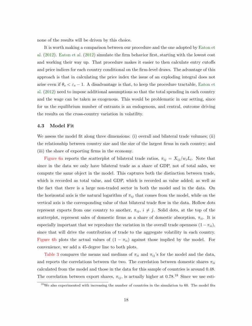
Figure 6a reports the scatterplot of bilateral trade ratios, πij = Xij/wiLi. Note that

since in the data we only have bilateral trade as a share of GDP, not of total sales, we

compute the same object in the model. This captures both the distinction between trade,

which is recorded as total value, and GDP, which is recorded as value added; as well as

the fact that there is a large non-traded sector in both the model and in the data. On

the horizontal axis is the natural logarithm of πij that comes from the model, while on the

vertical axis is the corresponding value of that bilateral trade flow in the data. Hollow dots

represent exports from one country to another, πij , i 6= j. Solid dots, at the top of the

scatterplot, represent sales of domestic firms as a share of domestic absorption, πii. It is

especially important that we reproduce the variation in the overall trade openness (1−πii),since that will drive the contribution of trade to the aggregate volatility in each country.

Figure 6b plots the actual values of (1 − πii) against those implied by the model. For

convenience, we add a 45-degree line to both plots.

Table 3 compares the means and medians of πii and πij ’s for the model and the data,

and reports the correlations between the two. The correlation between domestic shares πii

calculated from the model and those in the data for this sample of countries is around 0.48.

The correlation between export shares, πij , is actually higher at 0.78.18 Since we use esti-

18We also experimented with increasing the number of countries in the simulation to 60. The model fits

18

mated gravity coefficients together with the actual data on bilateral country characteristics

to compute trade costs, it is not surprising that bilateral trade flows implied by our model

are closely correlated to those in the data given the success of the empirical gravity relation-

ship. Nonetheless, since the gravity estimates we use come from outside of our calibration

procedure, it is important to check that our model delivers outcomes similar to observed

trade volumes.

We next assess whether the model reproduces the relationships between country size

and the relevant features of the firm size distributions demonstrated in Figure 3. In the

data, log country size is negatively and significantly related to the log Herfindahl index of

firm sales; and positively and significantly related to the size of the 10 largest firms and the

size of the largest firm in the economy. We can compare the data to the same relationships

inside our model. It turns out that in the model the elasticity of the Herfindahl index with

respect to country size is −0.135, which is right in between the Herfindahl-country size

elasticity of −0.114 (sample of countries with more than 1000 firms) and −0.284 (sample of

countries with more than 100 firms) in Figure 3a. Turning to the size of the largest firms,

our model produces an elasticity of the 10 largest firms to country size of 0.903, and of

the single largest firm to country size of 0.908. These are close to the range of elasticities

produced by the data: 0.888 to 1.006 for the 10 largest firms (Figure 3b), and 0.838 to 0.906

(Figure 3c) for the single largest firm.

Finally, we use the model solution to calculate the percentage of firms that export

in the total economy, as well as in the tradeable sector. In particular, the total number

of exporters in country i equals ITi ×(bT maxj 6=i

{aTji

})θT. The total number of firms

operating in the tradeable sector equals ITi ×(bT maxj

{aTji

})θT, and in the non-tradeable

sector INi ×(bNa

Nii

)θN . We would like to compare the export participation shares in the

model to what is found in the data. Unfortunately, there is no systematic empirical evidence

on these shares across countries (and time). However, we have examined available data and

existing literature and found these shares for 8 countries: U.S., Germany, France, Argentina,

Colombia, Ireland, Chile, and New Zealand. Table 4 compares the export participation

shares produced by the model to those found in the data in this subset of countries. The

first two columns report the values in the model, with the shares of exporters relative to all

the firms in the economy in column 1 and in the tradeable sector only in column 2. Data

the data well, but there are more zeros in bilateral trade data in the 60-country sample compared to the50-country one. (With 50 countries, among the 2500 possible unidirectional bilateral trade flows, only 18are zeros.) Since our model does not generate zero bilateral trade outcomes, we stick with the largest 49countries in our analysis.

19

sources differ across countries, in particular the shares of exporting firms are sometimes

reported only relative to all firms in the economy (which we record in column 3), and

sometimes relative to all the firms in the tradeable sector (which we record in column 4).

Thus, data in column 3 should be compared to model outcomes in column 1, while data in

column 4 should be compared to model outcomes in column 2.

In both the data and the model, larger countries tend to have fewer exporters relative to

the overall number of firms (compare U.S. to Colombia); countries closer to large markets

tend to have higher shares of exporters compared to faraway countries (compare Ireland to

New Zealand). In most cases the model implied value is close to the data. We should note

that by making ad hoc adjustments to trade costs in individual countries, we can match

each and every one of these numbers exactly. We do not do so because this information is

not available systematically for every country in our sample, and because the available firm-

level data themselves are noisy. Instead, we take trade costs as implied by a basic gravity

model, and the variation in fixed costs as implied by the Doing Business Indicators, an

approach that is rather straightforward and does not involve any manual second-guessing.

4.4 Main Results: Country Size and Trade Openness

As would be expected, the level of aggregate volatility in the model is lower than what is

observed in the data, since in the model all volatility comes from idiosyncratic shocks to

firms. Column 1 of Table 5 reports the ratio of the aggregate volatility implied by the model

to the actual GDP volatility found in the data. It ranges between 0.14 and 0.72, with a

value of 0.377 for the United States, almost identical to what Gabaix (2011) finds using

a very different methodology. Note that the variation in aggregate volatility in the model

across countries is generated by differences in country size as well as variation in bilateral

trade costs.

How well can the model reproduce the empirical relationship between aggregate volatility

and country size? Figure 7 plots volatility as a function of country size in the data and the

model. Note that since the level of aggregate volatility in the model does not match up

with the level in the data, this graph is only informative about the comparison of slopes,

not intercepts. In the data the elasticity of GDP volatility with respect to country size is

−0.139 (σGDP) in this sample of countries. Table A1 reports the results of estimating the

volatility-size relationship in the data for various country samples and with and without

controls. The baseline coefficient used in Figure 7 comes from the 50-country sample and

controlling for income per capita. Our calibrated model produces an elasticity of −0.135

20

(σT), which is extremely close to the one in the data though slightly below it in absolute

terms.

We now assess the contribution of international trade to aggregate volatility in our

sample of countries. Our model yields not only the aggregate volatility in the simulated

trade equilibrium, but also the aggregate volatility in autarky. As a preview of the results

on the impact of trade openness, Figure 7 reports the volatility-size relationship in autarky.

Without trade this relationship is somewhat flatter: the elasticity of volatility with respect

to country size in autarky is −0.115 (σA), lower than the −0.139 in the data. Thus, it

appears that openness helps the model match the slope of the size-volatility relationship:

without trade, smaller countries would be relatively less volatile than they actually are.

Column 2 of Table 5 reports the ratio of the volatility under the current trade regime

to the volatility in autarky in each country in the sample. In the table, countries are

ranked by size in descending order. We can see that international trade contributes very

little to overall GDP volatility in the U.S.. The country is so large and trade volumes are

so low (relative to total output) that its volatility under trade is only 1.035 times higher

than it would be in complete absence of trade. Similar results obtain for other very large

economies, such as Japan and China. By contrast, smaller, centrally located countries

experience substantially higher volatility compared to autarky. For instance, in a country

like Romania, the volatility under trade is some 22% higher than it would be in autarky,

and in Turkey, Denmark, and Norway it is 14-16% higher. In between are small, but remote

countries. South Africa, Argentina, and New Zealand experience aggregate volatility that

is about 10% higher than it would have been in autarky.

Finally, we investigate how well the model predicts the actual GDP volatility found in

the data. Table 6 presents regressions of actual volatility of per capita GDP growth over the

period 1970-2006 against the one predicted by the model (σT ), with all variables in natural

logs. Column 1 includes no controls. The relationship is positive and highly significant.

The fit of this simple bivariate relationship is remarkably high (R2 = 0.353), given that in

the model variation in σT is driven only by country size, trade barriers, and fixed costs. The

model uses no information on any type of aggregate shocks (TFP, monetary, or fiscal policy),

or any other country characteristics that have been shown to correlate with macroeconomic

volatility, such as per capita income, institutions, or industrial specialization. The second

column includes GDP per capita. The fit of the model improves slightly, and though the

coefficient on the model volatility is somewhat smaller, it remains significant at the 1%

level. The next two columns include measures of export structure volatility and sectoral

21

specialization, since di Giovanni and Levchenko (2009, 2012b) show that opening to trade

can impact aggregate volatility through changes in these variables. Column 3 adds the risk

content of exports, which captures the overall riskiness of a country’s export structure.19

The model volatility remains significant, and the R2 of the regression is now 0.477. Finally,

the fourth column adds a measure of production specialization for the manufacturing sector

(Herfindahl of sectoral production shares).20 The number of observations drops to 35 due

to limited data availability, but the model volatility still remains significant.

5 Robustness Checks and Model Perturbations

5.1 Free Entry and Intermediate Inputs

The assumption that the number of potential projects is determined by a free entry condition

may not be realistic. We thus simulate the quantitative model under the assumption that

the numbers of potential entrepreneurs Isi are fixed in every country and sector.21 Table 7

reports the results of this robustness check. For ease of comparison, the top row presents

the two main results from the baseline analysis. The first is that the model generates higher

volatility in smaller countries, with the elasticity of volatility with respect to country size of

−0.135. (As reported above, in the data this elasticity is very close, −0.139.) The second

key result of the paper is the contribution of trade openness to aggregate volatility. Column

2 reports the mean ratio of aggregate volatility under the current level of trade openness

relative to complete autarky.

Row 2 of Table 7 reports these two main results of the paper under the alternative

assumption that Isi is fixed. Not surprisingly, the elasticity of volatility with respect to

country size is virtually identical. Less obviously, the fixed-Isi model delivers very similar

changes in volatility due to trade openness: the mean impact is 9.0%, compared to 9.7%

with free entry.

A somewhat related question involves the role of intermediate input linkages. With

intermediate inputs, trade opening reduces the costs of the input bundle faced by firms,

making it easier to enter markets, all alse equal. To assess the importance of this effect,

we implement the baseline model with free entry but without intermediate input linkages:

19This measure is taken from di Giovanni and Levchenko (2012b). A country’s export structure can bevolatile due to a lack of diversification and/or exporting in sectors that are more volatile.

20This measure is calculated using the UNIDO database of sectoral production, and is taken from di Gio-vanni and Levchenko (2009).

21We set the values of Isi to be the same as in the free entry baseline, and adjust fii to match the 7 millionoperating firms in the U.S. in the trade equilibrium; the results are virtually the same if we instead adoptthe common ad hoc assumption that Isi are some constant fraction of Li, as in Chaney (2008), for instance.

22

βT = βN = 1. The two main results are presented in the third row of Table 7. The elasticity

of volatility with respect to country size is only slightly larger than in the baseline, at−0.145.

The impact of trade on volatility is much larger, at 23.8%.

5.2 Volatility Varying with Firm Size

An assumption that simplifies the analysis above is that the volatility of the proportional

change in sales, σ, does not change in firm size x. If the volatility of sales decreases

sufficiently fast in firm size, larger firms will be so much less volatile that they will not impact

aggregate volatility. In fact, an economy in which larger firms are just agglomerations of

smaller units each subject to i.i.d. shocks is not granular: shocks to firms cannot generate

aggregate fluctuations.

In practice, however, the negative relationship between firm size and its sales volatility

is not very strong. Several papers estimate the relationship between size and volatility of

the type σ = Ax−ξ using Compustat data (see, e.g., Stanley et al., 1996; Sutton, 2002).

The benchmark case in which larger firms are simply collections of independent smaller

firms would imply a value of ξ = 1/2, and the absence of granular fluctuations. Instead,

the typical estimate of this parameter is about 1/6, implying that larger firms are not

substantially less volatile than smaller ones.22 Gabaix (2011) argues that these estimates

may not be reliable, since they are obtained using only data on the largest listed firms. In

addition, it is not clear whether estimates based on the U.S. accurately reflect the experience

of other countries. Hence, our baseline analysis sets ξ = 0, and a value of σ based on the

largest 100 listed firms in the U.S.. In other words, we assume that all firms in the economy

experience volatility as low as the largest firms in the economy.

To check robustness of our results, we allow the firm-specific volatility to decrease in

firm size at the rate estimated in the literature. In that case, aggregate volatility is given

by

Stdz

(∆X

Ez (X)

)=

√√√√ I∑k=1

(Ax(k)−ξh(k))2,

22A related point concerns multi-product firms: if large firms sell multiple imperfectly correlated products,then the volatility of the total sales for multi-product firms will be lower than the volatility of single-productfirms. Evidence suggests, however, that even in multi-product firms the bulk of sales and exports is accountedfor by a single product line. Sutton (2002) provides evidence that in large corporations, the constituentbusiness units themselves follow a power law, with just a few very large business units and many muchsmaller ones. Along similar lines, Adalet (2009) shows that in the census of New Zealand firms, only about6.5% to 9.5% of sales variation is explained by the extensive margin (more products per firm), with the restexplained by the intensive margin (greater sales per product).

23

where, once again, x(k) is sales of firm k, while h(k) is the share of firm k’s sales in total

output in the economy.

The rest of the simulation remains unchanged. Since we are not matching the level

of aggregate volatility, just the role of country size and trade, we do not need to posit a

value of the constant A. However, it would be easy to calibrate to match the volatility

of the top 100 firms in the U.S. as reported by Gabaix (2011), for example. Note that

compared to the baseline simulation, modelling a decreasing relationship between firm size

and volatility is a double-edged sword: while larger firms may be less volatile as a result,

smaller firms are actually more volatile. This implies that the impact of either country size

or international trade will not necessarily be more muted when we make this modification

to the basic model.

Row 4 of Table 7 reports the two main results of the paper under the alternative as-

sumption that firm volatility decreases with firm size. In turns out that in this case, smaller

countries are even more volatile relative to large ones (the size-volatility elasticity doubles to

−0.286), and the contribution of trade is also larger, with trade leading to an average 29%

increase in volatility, compared to 9.7% in the baseline. Somewhat surprisingly, therefore,

allowing volatility to decrease in firm size implies a larger contribution of trade to aggregate

volatility, not a smaller one. In fact, this is the case in every country in the sample except

the U.S..23

5.3 Alternative Parameter Values

We assess the sensitivity of the results in two additional ways. The first is an alternative

assumption on the curvature of the firm size distribution. Eaton et al. (2011) estimate a

range of values for θ/(ε− 1) of between 1.5 and 2.5. Though Gabaix (2011) shows that the

shocks to large firms can still generate aggregate volatility when the power law exponent is

less than 2, it is important to check whether the main results of our paper survive under

alternative values of θ/(ε− 1). Row 5 of Table 7 presents the two main results of the paper

23Another possible determinant of firm volatility that would be relevant to our analysis is exporting.The baseline model assumes that the volatility of a firm’s sales growth does not change when it becomes anexporter. If exporters became systematically more or less volatile than non-exporters, the quantitative resultscould be affected. To check for this possibility, we used the Compustat Quarterly database of listed U.S.firms together with information on whether a firm is an exporter from the Compustat Segments database.Table A2 estimates the relationship between firm-level volatility – based on either the growth rate of sales ora measure of the “granular residual” following Gabaix (2011) – and its export status and size. Controllingfor size, export status is always insignificant, and even the magnitude of the coefficient is exceedingly small,implying that volatility of exporters is between 96 and 99% of the volatility of non-exporters. Furthermore,the estimated elasticity of volatility with respect to firm size is similar to what is reported in the literatureand used in the sensitivity check.

24

under the assumption that the slope of the power law in firm size is 1.5 instead of 1.06.

Though in each case the numbers are slightly smaller in absolute value, the main qualitative

and quantitative results remain unchanged: smaller countries still have lower volatility, with

elasticity of −0.123, and trade contributes slightly more to aggregate volatility, with the

average increase of 11.6%.

Second, we re-calibrate the model under two alternative values of ε, 4 and 8. In these

exercises, we continue to assume that the economy is characterized by Zipf’s Law, so that

θ/(ε − 1) is still equal to our baseline value of 1.06. Thus, as we change ε, we change θ

along with it. The results are presented in the last two rows of Table 7. The size-volatility

relationship is robust to these alternative assumptions. The elasticity of volatility with

respect to country size is similar to the baseline, though slightly lower when ε = 4. The

contribution of trade is quite similar as well, with 9.9% and 11.1% for ε = 4 and ε = 8,

respectively.

Although for all of the robustness checks Table 7 reports only the average impact of

trade, it turns out that all of these alternative implementations preserve the basic patterns

found in the baseline: trade raises volatility relative to autarky in all countries; larger

countries, and countries farther away from major trading partners tend to experience smaller

changes in volatility due to trade.

5.4 Further Reductions in Trade Costs

The analysis above compares aggregate volatility under today’s trade costs and in autarky,

and finds that the impact of trade on volatility has been robustly positive. We now evaluate

how volatility would change if trade costs decreased further from their current levels. Ta-

ble 8 presents the distribution of changes in aggregate volatility relative to its current level

for various magnitudes of trade cost reductions, from 10% to 75%. Strikingly, a further

reduction in trade costs leads to practically no change in volatility on average. For the

median country, a 50% reduction in trade costs increases volatility by only 1.1% relative to

the baseline. Furthermore, while the median volatility does rise slightly as trade costs fall,

the impact always ranges from positive to negative.

What can explain this non-monotonicity? Starting from autarky, as trade costs fall only

the largest firms export, and the distribution of firm size becomes more right-skewed. This

is the main mechanism responsible for the positive effect of trade openness on volatility.

However, as trade costs fall further, the exporting cutoff falls, and more and more firms

begin exporting. Eventually, this process will make the firm size distribution less fat-tailed:

25

when trade costs are so low that everyone exports, there is no selection into exporting, and

the power law in firm size exponent is the same as it was in autarky. Consistent with this

intuition, we find that the change in aggregate volatility when trade costs fall is closely

correlated with the concomitant change in the share of exporters. Smaller countries tend

to experience the largest increases in the share of exporters, and the greatest decreases in

volatility in this counterfactual. The opposite is true for the biggest countries.

Two additional points are worth making about the impact of further reductions in

trade costs. First, the non-monotonicity is not due to the assumption of free entry: the

results are virtually the same if we assume fixed Isi instead. Second, in the model without

intermediates the non-monotonicity disappears: reductions in trade costs always increase

volatility in that model. The source of the difference is that without intermediates, a given

fall in trade costs leads to a far smaller change in the exporting cutoffs than in the model

with intermediates. Many fewer firms enter the export markets, and thus the selection

into exporting effect is not reversed as it is in the baseline. What is the intuition for this

difference? In both models, a global fall in τij has the direct effect of lowering the firms’

marginal cost of serving the export markets, and thus makes the firm more likely to start

selling abroad. In a model with intermediates, there is an additional effect that the fall in

τij lowers the cost of the input bundle csj , since that input bundle includes foreign varieties

and those are now cheaper. This indirect effect further lowers the exporting cutoffs, over

and above the direct effect of τij . In the model without intermediates the indirect effect is

absent, since the input bundle is just the wage. It turns out that quantitatively this makes

a large difference for the results of a reduction in trade costs.

We conclude from these exercises that while the impact of openness on volatility at the

current levels of trade costs is robustly positive in all the models we consider, the outcomes of

further reductions in trade costs are sensitive to modelling assumptions about intermediate

input linkages.

6 Conclusion

Recent literature in both macroeconomics and international trade has focused attention on

the role of large firms. Gabaix (2011) demonstrates that if the distribution of firm size

follows a power law with an exponent close to negative 1 – which appears to be the case

in the data – the economy is granular: shocks to the largest firms can lead to aggregate

fluctuations.

This paper argues that the preponderance of large firms and their role in aggregate

26

volatility can help explain two empirical regularities: (i) smaller countries are more volatile,

and (ii) more open countries are more volatile. We calibrate and simulate a multi-country

model of firm-level production and trade that can generate granular fluctuations. The

model matches quite well a number of features of the data, such as observed bilateral and

overall trade volumes, export participation ratios, and the relative size of the largest firms

in different countries. We show that the model reproduces the elasticity of GDP volatility

with respect to country size found in the data. The contribution of international trade

to aggregate volatility varies a great deal depending on country characteristics. While it is

minimal in large, relatively closed economies like the U.S. or Japan, trade increases volatility

by up to 15-20% in small open economies such as Denmark or Romania.

Recent research incorporates heterogeneous firms into fully dynamic general equilib-

rium macroeconomics models, focusing on the impact of persistent aggregate shocks and

firm entry and exit (Ghironi and Melitz, 2005; Alessandria and Choi, 2007; Ruhl, 2008).

The importance of firm-specific idiosyncratic shocks for macroeconomic volatility via the

granular channel emphasized in this paper should be viewed as complementary to this work.

Future research incorporating these different mechanisms, as well as bringing disaggregated

data to the models, will help provide an even more complete picture of the macroeconomic

impact of trade integration.

Appendix A Data Description and Sources

Data on total GDP, per capita income, and trade openness come from the World Bank’s

World Development Indicators database (The World Bank, 2007b). Aggregate volatility

is the standard deviation of the yearly growth rates of per capita GDP in constant local

currency units over the period 1970-2006. Country size is the average share of the country’s

nominal U.S. dollar GDP in the world U.S. dollar GDP. Per capita income is the average

real PPP-adjusted per capita GDP. All the averages are taken over the same period over

which the volatility is computed, 1970-2006.

The figures on Fonterra are obtained from http://www.maf.govt.nz/mafnet/rural-nz/

profitability-and-economics/contribution-of-land-based-industries-nz-economic-growth/contribution07.

htm and http://tvnz.co.nz/view/page/423466/146647. The data on the 10 largest Korean

business groups come from the Korean Development Institute courtesy of Wonhyuk Lim,

and are for the year 2006.

The data on the Herfindahl indices of firm sales and the size of the 10 largest and the

single largest firm come from ORBIS, a large multi-country database published by Bureau

27

van Dijk that contains information on more than 50 million companies worldwide. The

data come from a variety of sources, including, but not limited to, registered filings and

annual reports. Importantly, the database includes both publicly traded and privately held

firms. The main variable used in the analysis is total sales. For each country, we use the

year with the most observations available, which is always between 2006 and 2008. ORBIS

is the largest available non-proprietary firm-level database. Nonetheless, coverage is quite

uneven across countries and years, implying that measures of concentration may not be

reliable or comparable across countries. We alleviate this concern by restricting the sample

of countries to those with a certain minimum numbers of firms, and by using indices that are

less prone to coverage-related biases. Di Giovanni and Levchenko (2012a) present a more

complete description of the ORBIS database and further evidence based on these data that

firm size distributions in a large number of countries are extremely fat-tailed.

To obtain values of τij , we use the gravity estimates from the empirical model of Helpman

et al. (2008). Combining geographical characteristics such as bilateral distance, common

border, common language, whether the two countries are in a currency union and others,

with the coefficient estimates reported by Helpman et al. (2008) yields, up to a multiplicative

constant, the values of τij for each country pair. We vary the multiplicative constant so as

to match the mean and median imports/GDP ratios observed in the data in our sample

of countries. Data on bilateral distance, common border, whether the country is an island

or landlocked, common language, and colonial ties are from Centre d’Etudes Prospectives

et Informations Internationales (CEPII). Data on legal origins come from La Porta et al.

(1998). Finally, information on currency unions and free-trade areas come from Rose (2004),

supplemented by internet searches whenever needed. The advantage of the Helpman et al.

(2008) estimates is that they are obtained in an empirical model that accounts explicitly

for both fixed and variable costs of exporting, and thus correspond most closely to the

theoretical structure in our paper. Note that in this formulation, τij = τji for all i and j.24

The values of fsii and fsij are calibrated following di Giovanni and Levchenko (2012a).

The Doing Business Indicators database (The World Bank, 2007a) collects information on

the administrative costs of setting up a firm – the time it takes, the number of procedures,

and the monetary cost – in a large sample of countries in the world. The particular variable

we use is the amount of time required to set up a business. We favor this indicator compared

to others that measure entry costs either in dollars or in units of per capita income, because

24An earlier version of the paper also computed τij using the estimates of Eaton and Kortum (2002) as arobustness check. The results were very similar.

28

in our model fsii is a quantity of inputs rather than a value. We must normalize f sii for

one country. Thus, we proceed by setting fsUS,US to a level just high enough to ensure an

interior solution for production cutoffs.25 Then, for every other country fsii is set relative

to the U.S.. To be precise, if according to the Doing Business Indicators database, it takes

10 times longer to register a business in country i than in the U.S., then fsii = 10× f sUS,US .

Since we do not have data on fixed costs of operating a business that vary by sector, we set

fsii to be equal in the N and T sectors.

To measure the fixed costs of international trade, we use the Trading Across Borders

module of the Doing Business Indicators. This module provides the costs of exporting a

20-foot dry-cargo container out of each country, as well as the costs of importing the same

kind of container into each country. Parallel to our approach to setting the domestic cost

fsii, the indicators we choose are the amount of time required to carry out these transactions.

This ensures that fTii and fTij are measured in the same units. We take the bilateral fixed

cost fTij to be the sum of the cost of exporting from country j and the cost of importing

into country i. The foreign trade costs fTij are on average about 40% of the domestic entry

costs fTii .26

The bilateral and overall trade volumes as a share of GDP used for comparison to the

model come from the Direction of Trade Statistics (International Monetary Fund, 2007).

Appendix B The Complete 2-Sector Model

In country i, consumers maximize

max{yNi (k),yTi (k)}

JNi∑k=1

yNi (k)εN−1

εN

αεNεN−1

JTi∑k=1

yTi (k)εT−1

εT

(1−α)εTεT−1

s.t.

JNi∑k=1

pNi (k) yNi (k) +

JTi∑k=1

pTi (k) yTi (k) = Yi,

25That is, we set fsUS,US to a level just high enough that asji < 1/bs for all i, j = 1, ..., C in all the baselineand counterfactual exercises, with 1/bs being the upper limit of the distribution of a.

26An earlier version of the paper was more agnostic about the nature of domestic fixed costs fTii , andassumed instead that they are equal (and low) in every country. The results were very similar. In addition,we carried out the analysis setting the bilateral fixed cost to be the sum of domestic costs of starting abusiness in the source and destination countries: fTij = fTii + fTjj . This approach may be preferred if fixedcosts of exporting involved more than just shipping, and required, for instance, the exporting firm to createa subsidiary for the distribution in the destination country. The results were virtually identical.

29

where ysi (k) is final consumption of good k belonging to sector s = N,T in country i, psi (k)

is the price of this good, Yi is total final consumption expenditure in the economy, and Jsi

is the number of varieties available in sector s in country i coming from all countries. Since

consumer preferences are Cobb-Douglas in CES aggregates of N and T , final consumption

expenditure on sector N is equal to αYi, and on the T sector, (1− α)Yi.

The CES composites of both N and T are used both as consumption and as intermediate

inputs in production. Let Xsi denote the total spending – final and intermediate – on sector

s = N,T in country i. Given this total expenditure, it is well known that expenditure on

an individual variety k in country i is equal to

xsi (k) =Xsi

(P si )1−εspsi (k)1−εs ,

where P si is the ideal price index of sector s in this economy, (2), augmented with the

appropriate sector superscripts.

Production in both sectors uses both labor and CES composites of N and T as inter-

mediate inputs. An input bundle in country j and sector s has a cost

csj = wβsj

[(PNj)ηs (

P Tj)1−ηs]1−βs

.

That is, production in sector s = N,T requires labor, inputs of N , and inputs of T . The

share of labor in value added, βs, and the share of non-tradeable inputs in total input usage,

ηs, both vary by sector.

Entrepreneurs can pay the exploration cost fe to enter either sector. Each entrepreneur

that entered sector s in country j decides whether or not to pay the fixed cost of production

fsjj , and which, if any, export markets to serve. In the N sector, we assume that trade costs

are infinite, and thus a firm in country j may only serve its own market.

The expressions defining the input requirement cutoffs asij , (3) and (4), and the free

entry conditions (5), have the same form (up to the appropriate sector superscripts) and

will hold in each sector. Following similar steps, we derive the expressions for the price

levels in the two sectors:

PNi =1

bN

[θN

θN − (εN − 1)

]− 1θN εN

εN − 1

(XNi

εN

)− θN−(εN−1)

θN (εN−1)

INi ( 1

cNi

)θN ( 1

cNi fNii

) θN−(εN−1)

εN−1

− 1θN

(B.1)

30

and

P Ti =1

bT

[θT

θT − (εT − 1)

]− 1θT εTεT − 1

(XTi

εT

)− θT−(εT−1)

θT (εT−1)

C∑j=1

ITj

(1

τijcTj

)θT (1

cTj fTij

) θT−(εT−1)

εT−1

− 1θT

.

(B.2)

Having expressed P si , and asij in terms of Xsi and csi for all i, j = 1, . . . , C, it remains to close

the model by solving for the Xsi ’s and wi’s. To do this, we impose balanced trade for each

country and the market clearing conditions in each sector and country. Free entry implies

that the total profits are zero, and thus final expenditure in country i simply equals labor

income: Yi = wiLi. Total expenditure XNi and XT

i equals final spending plus expenditure

on sector s as intermediate inputs in both sectors:

XNi = αwiLi + (1− βN ) ηNX

Ni + (1− βT ) ηTX

Ti

XTi = (1− α)wiLi + (1− βN ) (1− ηN )XN

i + (1− βT ) (1− ηT )XTi .

Note that even though the T sector has both imports and exports, the assumption that only

T -sector goods can be traded amounts to imposing balanced trade within the T sector, and

thus the second condition must be satisfied in equilibrium as written. These two conditions

imply that total spending in each sector is a constant multiple of labor income wiLi.

Total sales from country i to country j can be written as

XTji =

XTj(

P Tj

)1−εT(

εTεT − 1

τjicTi

)1−εTITi

bθTT θTθT − (εT − 1)

(aTji)θT−(εT−1)

.

Using expressions for aTji in (4), and P Tj in (B.2), total exports from i to j become

XTji =

ITi(τjic

Ti

)−θT (fTjicTi )− θT−(εT−1)

εT−1

∑Cl=1 I

Tl

(τjlc

Tl

)−θT (fTjlcTl )− θT−(εT−1)

εT−1

XTj .

Using the trade balance conditions, XTi =

∑Cj=1X

Tji for each i = 1, . . . , C, as well as the

property that total spending XTi is a constant multiple of wiLi leads to the following system

of equations in wi:

wiLi =

C∑j=1

ITi τ−θTji

(fTji)− θT−(εT−1)

εT−1

(wβTi

[(PNi)ηT (

PTi)1−ηT ]1−βT)−θT− θT−(εT−1)

εT−1

∑Cl=1 I

Tl τ−θTjl

(fTjl

)− θT−(εT−1)

εT−1

(wβTl

[(PNl)ηT (

PTl)1−ηT ]1−βT)−θT− θT−(εT−1)

εT−1

wjLj ,

(B.3)

31

i = 1, . . . , C. There are C − 1 independent equations in this system, with wage in one of thecountries as the numeraire.

A monopolistically competitive equilibrium is a set of prices{wi, P

Ni , P

Ti

}Ci=1

, and factorallocations such that (i) consumers maximize utility; (ii) firms maximize profits, and (iii)all goods and factor markets clear. The equilibrium is obtained as a solution to (C−1)+2×C+2×C equations in wi, P

Ni , P Ti , INi and ITi that satisfies equations (5) for both s = N,T ,

(B.1), (B.2), and (B.3) for each i = 1, . . . , C. We solve these equations numerically in orderto carry out the main quantitative exercise in this paper.

B.1 Calibrating To Zipf’s Law in Firm Size in a Two-Sector Model withTrade

While Section 3.2 argues that in a one-sector Melitz-Pareto economy, steady-state firm sizefollows a power law with exponent θ/(ε − 1), our quantitative model features two sectors,idiosyncratic shocks to firm sales, as well as selection into exporting. This section showsthat the aggregate model economy with these additional features will still exhibit Zipf’sLaw in firm size.

Deriving an aggregate power law in an economy with two sectors involves computingthe (counter-)cdf of the following mixture of distributions. Let Q be a random variablethat follows a power law with exponent ζ1 with probability p, and with exponent ζ2 withprobability 1 − p. It is straightforward to show that the counter-cdf of Q is equal to:Pr(Q > q) = pD1q

−ζ1 + (1− p)D2q−ζ2 . Importantly, when ζ1 = ζ2 = ζ, Q is itself a power

law with exponent ζ. This means that a two-sector economy in which both sectors followa power law with the same exponent will, in aggregate, also exhibit a power law with thatexponent. Our quantitative exercise adopt the assumption that both the N and T sectorsfollow Zipf’s Law. Though we are not aware of any comprehensive set of estimates of powerlaw exponents in both traded and non-traded sectors, di Giovanni et al. (2011) estimatepower law exponents for a wide range of both traded and non-traded industries using acensus of French firms, and find that power law exponents do not differ systematicallybetween traded and non-traded sectors. It still could be the case that while the reducedform exponents – which correspond to θT /(εT − 1) and θN/(εN − 1) – are the same, theactual values of θs and εs differ. Since we do not have reliable information about how thesetwo individual parameters differ across sectors, we adopt the most agnostic and neutralassumption that both θs and εs are the same in the two sectors.

Another concern is that even if steady-state firm size in the aggregate economy followsZipf’s Law, when firms are hit by idiosyncratic shocks z, the resulting distribution would besomething else. It turns out, however, that power laws are preserved under multiplicationby a random variable with finite variance. That is, if firm sales are driven by a randomproductivity that generates Zipf’s Law (1/a in our notation), and a finite variance shock(z), the resulting distribution of sales is still Zipf (Gabaix, 2009, pp. 258-259).

Another point regarding the calibration of power law parameters is that strictly speak-ing, when not all firms export, selection into exporting implies that the power law exponentestimated on total sales – domestic plus exporting – is lower than θ/(ε − 1). Di Giovanniet al. (2011) explore this bias in detail using the census of French firms, and suggest sev-eral corrections to the estimating procedure that can be used to estimate θ/(ε − 1) in an

32

internally consistent way. Their analysis shows that the bias introduced by selection intoexporting is not large. Corrected estimates obtained by di Giovanni et al. (2011) show thatθ/(ε− 1) is about 1.05, roughly the same as the value used in the quantitative exercise.

Thus, even though the model is enriched with these additional features, the resultingdistribution of firm size that the model produces still follows Zipf’s Law.

Appendix C Aggregate Volatility Derivation

Firm k in country i with unit input requirement a(k) and realization of transitory shockz(k) has sales of

xs(a(k), z(k)) =

C∑j=1

1 [a(k) ≤ aij ]Xsj(

P sj

)1−εs ( εsεs − 1

τjicsia(k)z(k)

)1−εs

=

C∑j=1

1 [a(k) ≤ aij ]Xsj(

P sj

)1−εs ( εsεs − 1

τjicsia(k)

)1−εs z, (C.1)

where 1 [·] is the indicator function that captures whether firm k serves market j, and z ≡z1−εs . We already assumed that Ez (z) = 1, and now we further suppose that Varz (z) = σ2.Expected sales for the firm with productivity a(k) are

Ez [xs(a(k), z(k))] =C∑j=1

1 [a(k) ≤ aij ]Xsj(

P sj

)1−εs ( εsεs − 1

τjicsia(k)

)1−εs. (C.2)

Given the expression for the actual sales of the firm with a transitory shock z(k) in (C.1)and the expected sales of the firm with productivity a(k) in (C.2), the actual sales as anapproximation around Ez [xs(a(k), z(k))] are

xs(a(k), z(k)) ≈ Ez [xs(a(k), z(k))] +dx

dz

∣∣∣∣z=1

∆z.

Therefore, the proportional change in xs(a(k), z(k)), or the growth rate, is given by

∆xs(a(k), z(k))

Ez (xs(a(k), z(k)))= z − 1,

and the variance of this growth rate is

Varz

(∆xs(a(k), z(k))

Ez (xs(a(k), z(k)))

)= σ2,

which we assume for simplicity is the same in the two sectors s = N,T . Dropping the sectorsuperscripts, the total sales in the economy are given by (8), thus the change in the totalsales relative to the non-stochastic steady state (the growth rate) is

∆X

EzX=

∑Ik=1 ∆x(a(k), z(k))

EzX=

I∑k=1

∆x(a(k), z(k))

Ez [x(a(k), z(k))]

Ez [x(a(k), z(k))]

EzX.

33

This means that the aggregate volatility is

Varz

(∆X

EzX

)= Varz

(I∑

k=1

∆x(a(k), z(k))

Ez [x(a(k), z(k))]

Ez [x(a(k), z(k))]

EzX

)

=I∑

k=1

Varz

(∆x(a(k), z(k))

Ez [x(a(k), z(k))]

)(Ez [x(a(k), z(k))]

EzX

)2

= σ2I∑

k=1

(Ez [x(a(k), z(k))]

EzX

)2

= σ2I∑

k=1

h(k)2,

where h(k) is the share of the firm k’s expected sales in total expected sales in the economy.As expected, the volatility of total output in the economy is equal to the volatility of anindividual firm’s output times the Herfindahl index of production shares.

References

Adalet, Muge, “Multi-Product Exporters and Product Turnover Behaviour of New ZealandFirms,” April 2009. New Zealand Treasury Working Paper 09/01.

Alessandria, George and Horag Choi, “Do Sunk Costs of Exporting Matter for Net ExportDynamics?,” Quarterly Journal of Economics, 2007, 122 (1), 289–336.

Alvarez, Fernando and Robert E. Lucas Jr., “General Equilibrium Analysis of the Eaton-Kortum Model of International Trade,” Journal of Monetary Economics, September 2007,54 (6), 1726–1768.

Anderson, James and Eric van Wincoop, “Trade Costs,” Journal of Economic Literature,2004, 42 (3), 691–751.

Arndt, Christian, Claudia Buch, and Anselm Mattes, “Barriers to Internationalization:Firm-Level Evidence from Germany,” September 2009. IAW Discussion Paper 52.

Axtell, Robert L., “Zipf Distribution of U.S. Firm Sizes,” Science, September 2001, 293(5536), 1818–1820.

Backus, David K., Patrick J. Kehoe, and Finn E. Kydland, “International Business Cycles:Theory and Evidence,” in Thomas Cooley, ed., Frontiers of Business Cycle Research,Princeton: Princeton University Press, 1995, pp. 331–356.

Barlevy, Gadi, “The Costs of Business Cycles Under Endogenous Growth,” American Eco-nomic Review, September 2004, 94 (4), 964–990.

Bernard, Andrew B., J. Bradford Jensen, and Peter Schott, “Falling Trade Costs, Hetero-geneous Firms, and Industry Dynamics,” April 2003. NBER Working Paper No. 9639.

Bernard, Andrew B., J. Bradford Jensen, Stephen Redding, and Peter Schott, “Firms inInternational Trade,” Journal of Economic Perspectives, 2007, 21, 105–130.

34

Blattman, Christopher, Jason Hwang, and Jeffrey G. Williamson, “Winners and Losersin the Commodity Lottery: The Impact of Terms of Trade Growth and Volatility inthe Periphery 1870–1939,” Journal of Development Economics, January 2007, 82 (1),156–179.

Bustos, Paula, “Trade Liberalization, Exports and Technology Upgrading: Evidence onthe impact of MERCOSUR on Argentinean Firms,” American Economic Review, March2011, 101 (1), 304–340.

Canals, Claudia, Xavier Gabaix, Josep M. Vilarrubia, and David E. Weinstein, “TradePatterns, Trade Balances, and Idiosyncratic Shocks,” 2007. la Caixa Working Paper02/2007.

Canning, D., L.A.N. Amaral, Y. Lee, M. Meyer, and H.E. Stanley, “Scaling the Volatilityof GDP Growth Rates,” Economics Letters, 1998, 60, 335–341.

Cebeci, Tolga, Ana M. Fernandes, Caroline Freund, and Martha Denisse Pierola, “ExporterDynamics Database,” May 2012. mimeo, The World Bank.

Chaney, Thomas, “Distorted Gravity: The Intensive and Extensive Margins of InternationalTrade,” American Economic Review, September 2008, 98 (4), 1707–1721.

Crucini, Mario J., “Country Size and Economic Fluctuations,” Review of InternationalEconomics, May 1997, 5 (2), 204–220.

Delli Gatti, Domenico, Corrado Di Guilmi, Edoardo Gaffeo, Gianfranco Giulioni, MauroGallegati, and Antonio Palestrini, “A New Approach to Business Fluctuations: Hetero-geneous Interacting Agents, Scaling Laws and Financial Fragility,” Journal of EconomicBehavior and Organization, April 2005, 56 (4), 489–512.

di Giovanni, Julian and Andrei A. Levchenko, “Trade Openness and Volatility,” Review ofEconomics and Statistics, August 2009, 91 (3), 558–585.

and , “Firm Entry, Trade, and Welfare in Zipf’s World,” June 2012. Forthcoming,Journal of International Economics.

and , “The Risk Content of Exports: a Portfolio View of International Trade,” NBERInternational Seminar on Macroeconomics, May 2012, 8 (1), 97–151.

, , and Romain Ranciere, “Power Laws in Firm Size and Openness to Trade: Measure-ment and Implications,” Journal of International Economics, September 2011, 85 (1),42–52.

Dixit, Avinash K. and Joseph E. Stiglitz, “Monopolistic Competition and Optimum ProductDiversity,” American Economic Review, June 1977, 67 (3), 297–308.

and , “Monopolistic Competition and Optimum Product Diversity: Reply,” AmericanEconomic Review, March 1993, 83 (1), 302–304.

Easterly, William, Roumeen Islam, and Joseph E. Stiglitz, “Shaken and Stirred: ExplainingGrowth Volatility,” in B. Pleskovic and N. Stern, eds., Annual World Bank Conferenceon Development Economics, 2001.

Eaton, Jonathan and Samuel S. Kortum, “Technology, Geography, and Trade,” Economet-rica, September 2002, 70 (5), 1741–1779.

, , and Francis Kramarz, “An Anatomy of International Trade: Evidence from FrenchFirms,” Econometrica, September 2011, 79 (5), 1453–1498.

35

, , and Sebastian Sotelo, “International Trade: Linking Micro and Macro,” February2012. NBER Working Paper No. 17864.

Fabling, Richard and Lynda Sanderson, “Firm Level Patterns in Merchandise Trade,” May2008. New Zealand Ministry of Economic Development Occasional Paper 08/03.

Fitzgerald, Doireann and Stefanie Haller, “Pricing-to-Market: Evidence From Plant-LevelPrices,” September 2010. Mimeo, Stanford University and ESRI.

Fujita, Masahisa, Paul Krugman, and Anthony J. Venables, The Spatial Economy: Cities,Regions, and International Trade, Cambridge, Mass.: The MIT Press, 2001.

Furceri, Davide and Georgios Karras, “Country Size and Business Cycle Volatility: ScaleReally Matters,” Journal of the Japanese and International Economies, 2007, 21 (4),424–434.

Gabaix, Xavier, “Power Laws in Economics and Finance,” Annual Reviews of Economics,2009, 1, 255–93.

, “The Granular Origins of Aggregate Fluctuations,” Econometrica, May 2011, 79 (3),733–772.

Gavin, Michael and Ricardo Hausmann, “Growth with Equity: The Volatility Connection,”in Nancy Birdsall, Carol Graham, and Richard H. Sabot, eds., Beyond Tradeoffs: Mar-ket Reforms and Equitable Growth in Latin America, Washington, DC: Inter-AmericanDevelopment Bank and the Brookings Institution, 1998, pp. 91–109.

Ghironi, Fabio and Marc J. Melitz, “International Trade and Macroeconomic Dynamics withHeterogeneous Firms,” Quarterly Journal of Economics, August 2005, 120 (3), 865–915.

Head, Allen C., “Country Size, Aggregate Fluctuations, and International Risk Sharing,”Canadian Journal of Economics, November 1995, 28 (4b), 1096–1119.

Helpman, Elhanan, Marc J. Melitz, and Yona Rubinstein, “Estimating Trade Flows: Trad-ing Partners and Trading Volumes,” Quarterly Journal of Economics, May 2008, 123 (2),441–487.

Holmes, Thomas J. and John J. Stevens, “An Alternative Theory of the Plant Size Distri-bution with an Application to Trade,” April 2010. Mimeo, University of Minnesota andFederal Reserve Board of Governors.

International Monetary Fund, “Directions of Trade Statistics,” 2007.

Katzenstein, Peter J., Small States in World Markets: Industrial Policy in Europe, Ithacaand London: Cornell University Press, 1985.

Koren, Miklos and Silvana Tenreyro, “Volatility and Development,” Quarterly Journal ofEconomics, February 2007, 122 (1), 243–287.

Kose, M. Ayhan, Eswar S. Prasad, and Marco E. Terrones, “Financial Integration andMacroeconomic Volatility,” IMF Staff Papers, 2003, 50 (Special Issue), 119–141.

Kraay, Aart and Jaume Ventura, “Comparative Advantage and the Cross-Section of Busi-ness Cycles,” Journal of European Economic Association, December 2007, 5 (6), 1300–1333.

Krugman, Paul, “Scale Economies, Product Differentiation, and the Pattern of Trade,”American Economic Review, 1980, 70 (5), 950–959.

36

La Porta, Rafael, Florencio Lopez de Silanes, Andrei Shleifer, and Robert W. Vishny, “Lawand Finance,” Journal of Political Economy, December 1998, 106 (6), 1113–1155.

Laursen, Thomas and Sandeep Mahajan, “Volatility, Income Distribution, and Poverty,” inJoshua Aizenman and Brian Pinto, eds., Managing Economic Volatility and Crises: APractitioner’s Guide, Cambridge University Press New York 2005, pp. 101–136.

Melitz, Marc J., “The Impact of Trade on Intra-Industry Reallocations and AggregateIndustry Productivity,” Econometrica, November 2003, 71 (6), 1695–1725.

Newbery, David M. G. and Joseph E. Stiglitz, “Pareto Inferior Trade,” Review of EconomicStudies, January 1984, 51 (1), 1–12.

OECD, “The Rise of China and India: What’s in it for Africa?,” Technical Report, Orga-nization of Economic Cooperation and Development, Development Centre Studies 2006.

Pallage, Stephane and Michel A. Robe, “On The Welfare Cost of Economic Fluctuations inDeveloping Countries,” International Economic Review, May 2003, 44 (2), 677–698.

Pavcnik, Nina, “Trade Liberalization, Exit, and Productivity Improvements: Evidence fromChilean Plants,” Review of Economic Studies, January 2002, 69 (1), 245–276.

Ramey, Garey and Valerie A. Ramey, “Cross-Country Evidence on the Link BetweenVolatility and Growth,” American Economic Review, December 1995, 85 (5), 1138–1151.

Rose, Andrew K., “Do We Really Know That the WTO Increases Trade?,” AmericanEconomic Review, March 2004, 94 (1), 98–114.

Ruhl, Kim J., “The International Elasticity Puzzle,” 2008. mimeo, NYU Stern School ofBusiness.

Stanley, Michael H.R., Luis A.N. Amaral, Sergey V. Buldyrev, Shlomo Havlin, HeikoLeschhorn, Philipp Maass, Michael A. Salinger, and H. Eugene Stanley, “Scaling Be-haviour in the Growth of Companies,” Nature, February 1996, 379, 804–806.

Sutton, John, “The Variance of Firm Growth Rates: the ‘Scaling’ Puzzle,” Physica A, 2002,312, 577–590.

The World Bank, “Doing Business Indicators,” 2007.

, “World Development Indicators,” 2007.

Yang, Xiaokai and Ben J. Heijdra, “Monopolistic Competition and Optimum Product Di-versity: Comment,” American Economic Review, March 1993, 83 (1), 295–301.

Yi, Kei-Mu and Jing Zhang, “Structural Change in an Open Economy,” April 2010. Mimeo,Federal Reserve Bank of Philadelphia and University of Michigan.

37

Table 1. Parameter Values for the Calibrated Model

Parameter Baseline Sourceε a 6 Anderson and van Wincoop (2004)

θ b 5.3 Axtell (2001): θε−1 = 1.06

α 0.65 Yi and Zhang (2010)

{βN , βT } {0.65, 0.35}1997 U.S. Benchmark Input-Output Table{ηN , ηT } {0.77, 0.35}

τijc,d 2.30 Helpman et al. (2008)

fiic 14.24 The World Bank (2007a); normalizing fUS,US

fijc 7.20 so that nearly all firms in the U.S. produce

fe 34.0To match 7,000,000 firms in the U.S.(U.S. Economic Census)

σ e 0.1Standard deviation of sales growth of the top100 firms in COMPUSTAT

Notes:a Robustness checks include ε = 4 and ε = 8.b Robustness checks include θ

ε−1= 1.5 and ε = 6, so that θ = 6.5.

c Average in our sample of 50 countries.d τij = τji. Trade costs are adjusted by a constant ratio to match the median-level of openness across the50-country sample.e Robustness checks include σ varying with firm sales: σ = Ax−ξ, where ξ = 1/6.

38

Table 2. Top 49 Countries and the Rest of the World in Terms of 2006 GDP

GDP/ GDP/Country World GDP Country World GDPUnited States 0.300 Indonesia 0.006Japan 0.124 South Africa 0.006Germany 0.076 Norway 0.006France 0.054 Poland 0.005United Kingdom 0.044 Finland 0.005Italy 0.041 Greece 0.004China 0.028 Venezuela, RB 0.004Canada 0.026 Thailand 0.004Brazil 0.021 Portugal 0.003Spain 0.020 Colombia 0.003India 0.017 Nigeria 0.003Australia 0.016 Algeria 0.003Russian Federation 0.015 Israel 0.003Mexico 0.015 Philippines 0.003Netherlands 0.015 Malaysia 0.002Korea, Rep. 0.011 Ireland 0.002Sweden 0.010 Egypt, Arab Rep. 0.002Switzerland 0.010 Pakistan 0.002Belgium 0.009 Chile 0.002Argentina 0.008 New Zealand 0.002Saudi Arabia 0.007 Czech Republic 0.002Austria 0.007 United Arab Emirates 0.002Iran, Islamic Rep. 0.007 Hungary 0.002Turkey 0.007 Romania 0.002Denmark 0.006 Rest of the World 0.027

Notes: Ranking of top 49 countries and the rest of the world in terms of 2006 U.S.$ GDP. We include HongKong, POC, and Singapore in Rest of the World. Source: The World Bank (2007b).

39

Table 3. Bilateral Trade Shares: Data and Model Predictions

Model DataDomestic sales as a share of GDP (πii)

mean 0.7900 0.7520median 0.7717 0.7921corr(model,data) 0.4783

Imports as a share of GDP (πij)mean 0.0043 0.0047median 0.0021 0.0047corr(model,data) 0.7799

Notes: This table reports the means and medians of domestic output (top panel), and bilateral trade (bottompanel), both as a share of domestic GDP, in the model and in the data. Source: International MonetaryFund (2007).

Table 4. Export Participation: Data and Model Predictions for Whole Economy andTradeable Sector

(1) (2) (3) (4)Model Data

Country Total Tradeable Total TradeableUnited States 0.010 0.018 0.040 0.150Germany 0.111 0.238 0.100 ...France 0.029 0.065 0.040 0.090Argentina 0.112 0.352 ... 0.422Colombia 0.148 0.548 ... 0.363Ireland 0.332 1.000 ... 0.740Chile 0.095 0.335 0.105 ...New Zealand 0.062 0.189 0.051 0.135

Notes: This table compares, for selected countries, the share of exporters among all firms in the model(column 1) and the share of exporters among the tradeable sector firms in the model (column 2) withavailable estimates of corresponding shares in existing literature. Since for some countries, data are reportedrelative to all the firms in the economy, while for other countries it is reported relative to all the firms inthe traded sector, column 3 (data) should be compared to column 1 (model), and column 4 (data) shouldbe compared to Column 2 (model). For the United States, data are imputed based on publicly availableU.S. Economic Census data on the numbers of firms by sector, together with the summary statistics for thenumbers of exporters reported in Bernard et al. (2007). Data for France is based on authors’ calculationsusing the French Census data in di Giovanni et al. (2011). Data for Germany are from Arndt et al. (2009)(Table A2). Data for Argentina come from Bustos (2011), Table D.1. For New Zealand, data come fromFabling and Sanderson (2008), Table 4. Data on Ireland come from Fitzgerald and Haller (2010), Table 1.Data for Chile come from private communication with Miguel Fuentes at the Central Bank of Chile. Datafor Colombia come from private communication with Jorge Tovar at the Universidad de los Andes.

40

Table

5.

Inte

rnat

ion

alT

rad

ean

dA

ggre

gate

Vol

atil

ity

(1)

(2)

(1)

(2)

Tra

de/

Tra

de/

Tra

de/

Tra

de/

Cou

ntr

yA

ctu

alA

uta

rky

Cou

ntr

yA

ctu

alA

uta

rky

Un

ited

Sta

tes

0.37

71.

035

Ind

ones

ia0.

376

1.06

0Jap

an0.

405

1.01

4S

outh

Afr

ica

0.53

51.

109

Ger

man

y0.

582

1.08

0N

orw

ay0.

716

1.13

7F

ran

ce0.

559

1.09

8P

olan

d0.

377

1.11

4U

nit

edK

ingd

om0.

476

1.07

6F

inla

nd

0.43

71.

109

Ital

y0.

463

1.09

8G

reec

e0.

414

1.11

6C

hin

a0.

280

1.02

4V

enez

uel

a,R

B0.

285

1.07

0C

anad

a0.

446

1.07

7T

hai

lan

d0.

337

1.09

9B

razi

l0.

311

1.04

5P

ortu

gal

0.37

91.

068

Sp

ain

0.55

01.

061

Col

omb

ia0.

646

1.11

8In

dia

0.37

11.

064

Nig

eria

0.27

41.

172

Au

stra

lia

0.51

31.

051

Alg

eria

0.27

11.

156

Ru

ssia

nF

eder

atio

n0.

144

1.09

9Is

rael

0.51

31.

131

Mex

ico

0.32

91.

052

Ph

ilip

pin

es0.

439

1.10

7N

eth

erla

nd

s0.

693

1.10

4M

alay

sia

0.37

11.

095

Kor

ea,

Rep

.0.

296

1.05

9Ir

elan

d0.

457

1.08

7S

wed

en0.

634

1.09

9E

gyp

t,A

rab

Rep

.0.

513

1.19

2S

wit

zerl

and

0.54

81.

107

Pak

ista

n0.

630

1.16

5B

elgi

um

0.71

31.

072

Ch

ile

0.26

21.

119

Arg

enti

na

0.21

91.

091

New

Zea

lan

d0.

531

1.11

4S

aud

iA

rab

ia0.

168

1.06

9C

zech

Rep

ub

lic

0.33

01.

095

Au

stri

a0.

716

1.06

6U

nit

edA

rab

Em

irat

es0.

178

1.08

9Ir

an,

Isla

mic

Rep

.0.

189

1.09

7H

un

gary

0.39

91.

114

Tu

rkey

0.25

41.

157

Rom

ania

0.24

21.

218

Den

mar

k0.

612

1.15

6

Note

s:‘T

rade/

Act

ual’

rep

ort

sth

era

tio

of

aggre

gate

vola

tility

implied

by

the

model

under

trade

toth

eact

ual

vola

tility

of

per

capit

aG

DP

gro

wth

.In

calc

ula

ting

vola

tility

inth

em

odel

,th

isco

lum

nass

um

esth

at

the

standard

dev

iati

on

of

firm

-lev

elsa

les

gro

wth

rate

iseq

ual

toσ

=0.1

.‘T

rade/

Auta

rky’

rep

ort

sth

era

tio

of

vola

tility

inth

em

odel

under

trade

toth

evola

tility

under

auta

rky

for

each

countr

y.“A

ggre

gate

vola

tility

”re

ferr

ing

toei

ther

the

model

or

the

data

stands

for

the

standard

dev

iati

on

of

the

aggre

gate

gro

wth

rate

.

41

Table 6. Aggregate Volatility: Data and Model Predictions

(1) (2) (3) (4)Dep. Var: Log(GDP Volatility)

Log(σT ) 1.578** 1.365** 1.099** 0.765**(0.244) (0.321) (0.287) (0.274)

Log(GDP per capita) -0.093 -0.098 -0.146*(0.073) (0.065) (0.060)

Log(Risk Content of Exports) 0.100+ -0.064(0.053) (0.052)

Log(Herfindahl of Production) -0.134(0.217)

Constant 3.490** 3.417** 2.994** 0.282(1.092) (1.145) (1.079) (1.045)

Observations 49 49 47 35R2 0.353 0.378 0.477 0.450

Notes: The dependent variable is the standard deviation of per capita GDP growth over the period 1970-2006. σT is the aggregate volatility implied by the simulated model. GDP per capita is the PPP-adjustedper capita GDP. Risk Content of Exports is the measure of the volatility of a country’s export pattern takenfrom di Giovanni and Levchenko (2012b). Herfindahl of Production is the Herfindahl index of industry-levelproduction shares, taken from di Giovanni and Levchenko (2009). Robust standard errors in parentheses.+ significant at 10%; * significant at 5%; ** significant at 1%.

Table 7. Sensitivity Checks: The Impact of Country Size and Trade on Volatility

(1) (2)βSize Trade/Autarky

Baseline -0.135 1.097

Fixed Isi -0.133 1.090βT = βN = 1 -0.145 1.238σ = Ax−ξ -0.286 1.291ζ = 1.5 -0.123 1.116ε = 4 -0.119 1.099ε = 8 -0.138 1.111

Notes: This table reports (1) the coefficient of regressing the log of aggregate volatility on the log of countrysize (βSize) in the trade equilibrium, and (2) the contribution of international trade to aggregate volatility(the mean ratio of volatility under trade to the volatility in autarky) under alternative assumptions. Row 1reports the results for the baseline trade equilibrium simulation. Row 2 reports the results of a simulationwithout free entry. Row 3 reports the results of a simulation without intermediates. Row 4 reports theresults of a simulation in which the firm-specific volatility decreases in firm size. Row 5 reports the resultsof applying a power law coefficient of 1.5 rather than the baseline of 1.06. Rows 6 and 7 report the resultswhen using an elasticity of substitution of 4 or 8, respectively.

42

Table 8. The Impact of Further Reductions in Trade Costs on Aggregate Volatility

(1) (2) (3) (4)Percentage Reduction in Trade Costs10% 25% 50% 75%

Percentile5 0.998 0.994 0.984 1.003

10 0.998 0.998 0.991 1.00625 1.001 1.003 1.001 1.01750 1.004 1.011 1.011 1.03475 1.011 1.022 1.036 1.07595 1.019 1.036 1.055 1.129

min 0.995 0.988 0.973 0.990max 1.030 1.050 1.084 1.167

Notes: This table reports percentiles and minimum and maximum of the ratio of aggregate volatility undera four reductions in iceberg trade costs τij to the aggregate volatility as implied by the model under currenttrade costs.

43

Figure 1. Country Size and Aggregate Volatility

10 5 10 4 10 3 10 2 10 1 10010 2

10 1

Country Size Relative to the World (GDP Share)

GD

P Vo

latil

ity

Notes: This figure reports the partial correlation plot of aggregate volatility, measured as the standarddeviation of the annual growth rate of per capita GDP over 1970-2006, on the y-axis against country sizeon the x-axis, after netting out the impact of per capita income. Both axes are in log scale. Source: TheWorld Bank (2007b).

44

Figure 2. Korean Business Groups’ Sales As a Share of GDP and Total Exports

0%

5%

10%

15%

20%

25%

Samsung Hyundai Motor Co.

SK LG Korea Electric Power

Corporation

POSCO Lotte KT Korea Housing

Corporation

Korea Highway

Corporation

Sales/GDP Exports/Total Exports

Notes: This figure reports the 2006 sales of the top 10 Korean business groups, as a share of Korean GDP(blue/dark bars) and total Korean exports (red/light bars). Source: Korean Development Institute.

45

Figure 3. Country Size, Firm Sales Concentration, and Size of Large Firms

10−6 10−5 10−4 10−3 10−2 10−1 10010−2

10−1

100

Country Size Relative to the World (GDP Share)

Her

finda

hl In

dex

of F

irm S

ales

All ` = −0.305s.e. = 0.017 N = 139 R2 = 0.609

obs(S)* 1000 ` = −0.114s.e. = 0.037 N = 52 R2 = 0.161

obs(S)* 100

` = −0.284s.e. = 0.038 N = 81 R2 = 0.377

(a) Country Size and Firm Herfindahl Indices

10−6 10−5 10−4 10−3 10−2 10−1 100104

105

106

107

108

109

1010

Country Size Relative to the World (GDP Share)

Sale

s of

10

Larg

est F

irms

obs(S)* 1000

obs(S)* 100 ` = 0.933s.e. = 0.047 N = 81 R2 = 0.770

` = 0.888s.e. = 0.049 N = 52 R2 = 0.800

All ` = 1.006s.e. = 0.059 N = 139 R2 = 0.753

(b) Country Size and the Size of the 10 Largest Firms

Notes: These figures present the scatterplots of log country size and (a) the log Herfindahl index of firmsales; (b) the log size of the 10 largest firms, and (c) the log size of the largest firm, in all cases after nettingout per capita GDP. The countries with more than 1000 firms with sales data are labeled with ♦’s; thecountries with between 100 and 1000 firms with sales data are labeled with �’s, and the countries with lessthan 100 firms with sales data with ◦’s. The regression lines through the samples of (i) all countries; (ii)countries with ≥100 firms; and (iii) countries with ≥1000 firms are plotted through the data. Both axes arein log scale. Sources: ORBIS and The World Bank (2007b).

46

Figure 3. Country Size, Firm Sales Concentration, and Size of Large Firms (Cont’d)

10−6 10−5 10−4 10−3 10−2 10−1 100103

104

105

106

107

108

109

Country Size Relative to the World (GDP Share)

Sale

s of

Lar

gest

Firm

obs(S)* 100 ` = 0.838s.e. = 0.062 N = 81 R2 = 0.642

obs(S)* 1000

` = 0.865s.e. = 0.057 N = 52 R2 = 0.726

All ` = 0.906s.e. = 0.065 N = 139 R2 = 0.665

(c) Country Size and the Size of the Largest Firm

Notes: These figures present the scatterplots of log country size and (a) the log Herfindahl index of firmsales; (b) the log size of the 10 largest firms, and (c) the log size of the largest firm, in all cases after nettingout per capita GDP. The countries with more than 1000 firms with sales data are labeled with ♦’s; thecountries with between 100 and 1000 firms with sales data are labeled with �’s, and the countries with lessthan 100 firms with sales data with ◦’s. The regression lines through the samples of (i) all countries; (ii)countries with ≥100 firms; and (iii) countries with ≥1000 firms are plotted through the data. Both axes arein log scale. Sources: ORBIS and The World Bank (2007b).

47

Figure 4. The Timing of the Economy

-

Each entrant k = 1, . . . , Ifinds out its type a, anddecides whether or not toproduce and export

Those that decideto enter/export paythe fixed costs ofproducing/exporting

Existing producerslearn the transitoryshock z

Produce withunit input req. az;consume;markets clear

Figure 5. The Analytical Power Law in the Melitz-Pareto Model

Autarky!

Log(q)

Log(P{Sales>q})

Trade: 2-Country

Trade: C-Country

Notes: This figure depicts the distribution of firm size, measured by sales, and how it changes as it movesfrom Autarky to a 2-Country Trade equilibrium, and finally to a C-Country Trade equilibrium. In the two-country case, there is a single productivity cutoff, above which firms export abroad. Compared to autarky,there is a higher probability of finding larger firms above this cutoff. In the C-country case, with multipleexport markets there will be cutoffs for each market, with progressively more productive firms exporting tomore and more markets and growing larger and larger relative to domestic GDP.

48

Figure 6. Bilateral Trade Shares and Trade Openness: Data and Model Predictions

10 6 10 5 10 4 10 3 10 2 10 1 10010 6

10 5

10 4

10 3

10 2

10 1

100

Model Bilateral Trade Share ( ij)

Dat

a Bi

late

ral T

rade

Sha

re (

ij)

(a) Bilateral Trade Shares

0 0.1 0.2 0.3 0.4 0.5 0.6 0.7 0.80

0.1

0.2

0.3

0.4

0.5

0.6

0.7

0.8

USA

GBR

AUT

BEL

DNK

FRADEU

ITA

NLD

NOR

SWE

CHECAN

JPN

FINGRC

IRLPRT

ESP

TUR

AUS

NZLZAF

ARGBRA

CHL

COL

MEX

VEN

IRN

ISR

SAU

ARE

EGY

IND

IDN

KOR

MYS

PAK

PHLTHA

DZANGA

RUS

CHN

CZE

HUN

POL

ROM

Model Openness

Dat

a O

penn

ess

(b) Trade Openness

Notes: Figure (a) reports the scatterplot of domestic output (πii) and bilateral trade (πij), both as ashare of country i GDP. Solid dots represent observations of πii, while hollow dots represent bilateral tradeobservations (πij). Both axes are in log scale. Figure (b) reports the scatterplot of total imports as a shareof GDP. In both figures, the values implied by the model are on the horizontal axis; actual values are onthe vertical axis, and the line through the data is the 45-degree line. Source: International Monetary Fund(2007).

49

Figure 7. Volatility and Country Size: Data and Model Predictions

10 3 10 2 10 1 100

10 1.9

10 1.8

10 1.7

10 1.6

10 1.5

10 1.4

10 1.3

10 1.2

10 1.1

Country Size Relative to the World (GDP Share)

Dat

a an

d M

odel

Vol

atilit

ies

()

Autarky ( A): = 0.115Trade ( T): = 0.135

Data ( GDP): = 0.139

Notes: This figure plots the relationship between country size and aggregate volatility implied by the data(conditioning on per capita GDP), the model under trade, and the model in autarky. The dots representactual observations of volatility. Note that the data points and regression line are shifted by a constant forease of visual comparability with the model regressions lines. Source: The World Bank (2007b).

50

Table A1. Aggregate Volatility and Country Size Regressions

(1) (2) (3) (4) (5) (6)

Dep. Var: Log(GDP Volatility)

Log(Size) -0.177** -0.139** -0.090+ -0.209** -0.180** -0.142**(0.038) (0.044) (0.045) (0.035) (0.027) (0.023)

Log(GDP per capita) -0.157* -0.261** -0.049 -0.019 0.018(0.069) (0.070) (0.057) (0.045) (0.037)

Constant -4.352** -2.696** -1.533+ -4.010** -4.154** -4.291**(0.190) (0.763) (0.773) (0.601) (0.473) (0.410)

Observations 49 49 30 75 100 143R2 0.192 0.273 0.337 0.328 0.296 0.225

Notes: The dependent variable is the log of the standard deviation of per capita GDP growth over the period1970-2006. Size is a country’s GDP as a share of world GDP; GDP per capita is PPP-adjusted per capitaincome. All right-hand side variables are averages over 1970-2006. Robust standard errors in parentheses;+ significant at 10%; * significant at 5%; ** significant at 1%.

51

Table A2. U.S. Evidence on Relationship between Firm-Level Volatility and ExporterStatus and Size

(A) Sample period: 1980-2007Growth Granular

(1) (2) (1) (2)All Restricted All Restricted

Exporter -0.022 -0.014 -0.024 -0.017(0.021) (0.022) (0.021) (0.023)

Log(Sales) -0.129** -0.135** -0.128** -0.133**(0.005) (0.005) (0.005) (0.004)

Observations 15,901 14,597 15,859 14,558Number of SIC 440 415 427 403R2 0.181 0.183 0.198 0.201

(B) Sample period: 1980-1989Growth Granular

(1) (2) (1) (2)All Restricted All Restricted

Exporter -0.020 -0.013 -0.010 -0.013(0.021) (0.023) (0.020) (0.023)

Log(Sales) -0.128** -0.133** -0.126** -0.133**(0.005) (0.006) (0.004) (0.006)

Observations 8,529 7,693 8,509 7,693Number of SIC 435 410 422 410R2 0.171 0.170 0.181 0.170

(C) Sample period: 1990-2007Growth Granular

(1) (2) (1) (2)All Restricted All Restricted

Exporter -0.025 -0.021 -0.041 -0.036(0.029) (0.031) (0.029) (0.031)

Log(Sales) -0.136** -0.140** -0.134** -0.140**(0.008) (0.008) (0.008) (0.007)

Number of SIC 409 386 398 375Observations 6,881 6,467 6,857 6,443R2 0.149 0.151 0.165 0.174

Notes: This table presents the results from regressing a measure of firm-level sales volatility on measures ofits export status (‘Exporter’) and size (‘Sales’). Columns (1) and (2) (‘Growth’) take the natural logarithmof the standard deviation of firm real sales as the dependent variable. Columns (3) and (4) (‘Granular’) usea granular volatility measure, calculated as the standard deviation of the estimated residuals, εist, from thefollowing firm-level panel regression: ∆ log (Salesist) = αi+αst+εist, where i is a firm, s is a sector, and t isa quarter, so that αi is a firm-level effect, and αst is a sector×time effect. Standard deviations are calculatedover the given sample period, while export status and measures of firm size are averaged over the period.Regressions include sector-level fixed effects at the 4-digit SIC. ‘All’ includes all firms, while ‘Restricted’excludes firms in the commodity, energy, and public sectors. Data are taken from the Compustat Quarterlydatabase of listed U.S. firms together with information on whether a firm is an exporter from the CompustatSegments database. Robust standard errors in parentheses; + significant at 10%; * significant at 5%; **significant at 1%. 52