trade, exchange rate, and agricultural pricing policies in...
TRANSCRIPT

8505VOL. 2
WORLD BANKCOMPARATIVE STUDIES I
Trade, Exchange Rate,and Agricultural Pricing Policiesin ChileVolume II Appendixes: Data and Methodology
Alberto Valdes, qEugenia Muchnik, andHernan Hurtado
Ad-
;X_ tA


Trade, Exchange Rate,and Agricultural Pricing Policies
in ChileVolume II Appendixes: Data and Methodology
Alberto Valdes,Eugenia Muchnik, and
Hernan Hurtado
WORLD BANKCOMPARATIVE STUDIES
The World BankWashington, D.C.

Copyright i) 1990The International Bank for Reconstructionand Development/THE WORLD BANK
1818 H Street, N.W.Washington, D.C. 20433
All rights reservedManufactured in the United States of AmericaFirst printing February 1990
World Bank Comparative Studies are undertaken to increase the Bank's capacity to offer soundand relevant policy recommendations to its member countries. Each series of studies, of which ThePolitical Economy of Agricultural Pricing Policy is one, comprises several empirical, multicountryreviews of key economic policies and their effects on the development of the countries in which theywere implemented. A synthesis report on each series will compare the findings of the studies ofindividual countries to identify common patterns in the relation between policy and outcome-thusto increase understanding of development and economic policy
The series The Political Economy of Agricultural Pricing Policy, under the direction of Anne0. Krueger, Maurice Schiff, and Alberto Valdes, was undertaken to examine the reasons underlyingpricing policy, to quantify the systematic and extensive intervention of developing countries in thepricing of agricultural commodities during 1960-85, and to understand the effects of suchintervention over time. Each of the eighteen country studies uses a common methodology tomeasure the effect of sectoral and economywide price intervention on agricultural incentives andfood prices, as well as their effects on output, consumption, trade, intersectoral transfers,government budgets, and income distribution. The political and economic forces behind priceintervention are analyzed, as are the efforts at reform of pricing policy and their consequences.
The findings, interpretations, and conclusions in this series are entirely those of the authors andshould not be attributed in any manner to the World Bank, to its affiliated organizations, or tomnembers of its Board of Executive Directors or the countries they represent.
The rnaterial in this publication is copyrighted. Requests for permission to reproduce portions of itshould be sent to Director, Publications Department, at the address shown in the copyright noticeabove. The World Bank encourages dissemination of its work and will normally give permnissionpromptly and, when the reproduction is for noncommercial purposes, without asking a fee.Permiission to photocopy portions for classroom use is not required, though notification of such usehaving been made will be appreciated.
The complete backlist of World Bank publications is shown in the annual Index of Publications,which contains an alphabetical title list and indexes of subjects, authors, and countries and regions;it is of value principally to libraries and institutional purchasers. The latest edition is available freeof charge from Publications Sales Unit, Department F, The World Bank, 1818 H Street, N.W.,Washington, D.C. 20433, U.S.A., or from Publications, The World Bank, 66, avenue d'1ena, 75116Paris, France.
Alberto Valdes is an economist with the Intemational Food Policy Research Institute,Washington, D.C.; Eugenia Muchnik and Hernan Hurtado are economnists in the Department ofAgricultural Economnics of the Catholic University, Santiago, Chile; all are consultants to theWorld Bank.
Library of Congress Cataloging-in-Publication Data
Valdes, Alberto, 1935-Trade, exchange rate, and agricultural pricing policies In Chile /
Alberto Valdes, Eugenia Muchnik, Hernan Hurtado.p. cm. -- (The political economy of agricultural pricing
policy)Includes bibliographical references (v. 1, p. )Contents: v. 1. The country study -- v. 2. Appendixes: data and
methodology.ISBN 0-8213-1452-1 (v. 1). -- ISBN 0-8213-1453-X (v. 2)1. Agriculture and state--Chile. 2. Protectionism--Chile.
3. Foreign exchange administration--Chile. 4. Agricultural pricesupports--Chile. I. Muchnik, Eugenla, 1947- . II. Zeballos H.,Hernan (Zeballos Hurtado) III. Title. IV. Series: World Bankcomparative studies. Polltical economy of agricultural pricingpolicy.HD1878.V35 1990338.1'8--dc2O 90-12075
CIP
Abstract
Chile is a middle income country, with a predominantly urban population.Agriculture has played a changing role in the Chilean economy since approximatelyWorld War II. While the sector was perceived as having an enormous growthpotential, it was not a major factor in economic growth until the 1970s. Its sharein GNP was around 10 percent and it had a substantial agricultural trade deficit,while on the other hand provided employment to over 25 percent of the labor force inthe 1960s, declining to 17 percent in the 1970s.
The 24-year period covered by this study was marked by radical shifts ineconomic policies. Following fairly conservative policies in 1960-64, a drasticagrarian reform was implemented during 1965-70. This was followed by a socialistsystem during 1970-73 which was replaced by a military government. This lastgovernment carried out an ambitious experiment in trade liberalization and otherreforms reducing the role of the government in the economy.
The agricultural growth potential has been confirmed. Chile's agriculturaltrade deficit of U.S. $420 millions in 1975 evolved into a trade surplus of U.S.$1,090 millions in 1987, causing agricultural export revenues to rise from 1.9percent to 12.9 percent of total export revenues, simultaneously with a significantincrease in production of major import-competing crops, such as wheat, rice, andmaize.
The study found wide variations in direct nominal and effective rates ofprotection among the five products examined. There was consistent positive nominalprotection for milk production throughout the period, compared with persistenttaxation of beef prior to 1975. Nominal protection of wheat production waspositive, while apples and grapes experienced positive protection before 1975(benefitting from export subsidies) and had no protection thereafter. Effectiveprotection was also computed. Overall, policy reforms implemented between 1974 and1978 resulted in a significant decline in direct intervention, except for wheatproduction. While varying with world prices, rates of price intervention were lowerbetween 1975 and 1984 than they were between 1960 and 1974.
A notable finding of this study is that indirect intervention from exchangerate misalignment and industrial protection has a much greater impact on thestructure of incentives for Chilean agriculture than agricultural policies did. Inyears when direct intervention produced positive protection, indirect interventionled to lower, or often negative total protection.
The analysis on the experience of policies reforms in Chile affectingagricultural prices suggests a trade-off between i) agricultural terms of trade; ii)real wages in the urban sector; iii) returns to capital in the nonfarm sector; iv)foreign borrowing; and v) the supply of domestic subsidized credit. Reforms lead toshort-run losses of income to certain groups, and the study identifies importantconsideration with relation to the feasibility of agricultural trade liberalization.The study presents estimates of the magnitude of these losses, and examines themagnitude of additional resources needed to compensate those groups for their lossesduring the transition period, to make the reform more likely to succeed.


TABLE OF CONTENTS
List of Tables and Figures
Appendix I: ESTIMATION OF DIRECT PRICE INTERVENTION 1
ADJUSTMENT FOR BORDER PRICES 1- Wheat 1- Cattle 2- Apples and Grapes 7- Wholesale Prices of Powdered Milk 7
METHODOLOGY ON MEASURING DIRECT PRICE INTERVENTION 8- Wheat Adjustments 8- Milk Adjustments 13- Cattle Adjustments 22- Apples and Grapes 26
Appendix II: THE EQUIVALENT TARIFF ESTIMATION 42
THE MODEL 42EQUIVALENT TARIFF ESTIMATION 45
Appendix III: ESTIMATION PROCEDURE FOR PNA/PNA 51
APPROACH 51DATA SOURCES 53
Appendix IV: ESTIMATION OF THE EFFECTIVE RATE OF PROTECTION 55
THE METHOD 55ESTIMATION OF EFFECTIVE RATE OF PROTECTION IN AGRICULTURE (ERPA) 57DATA USED -59
- Prices 59- Import Tariffs 59- Real Exchange Rate Misalignment 61- Input-Output Coefficients 61
ESTIMATION OF THE EFFECTIVE RATE OF PROTECTION OF NONAGRICULTURE(ERPNA) 61
-Estimation of DAA for the Rest of the Period 1960-84 65- Tariffs Used for Exporting Sectors 66- Tariffs Used for Import Competing Sectors 66- Price Indexes Used 69- The Value of ac- 70- Real Exchange Rate Adjustments 71

vi
Page
METHODOLOGICAL LIMITATIONS 71- Ranking of Tariffs 71- The Treatment of Nontradables 72
Appendix V: THE SUPPLY RESPONSE MODEL: THEORETICAL FRAMEWORK 82
PRODUCTIVE RESOURCES 82SHORT RUN CONSTRAINTS IMPOSED BY PRODUCTIVE RESOURCES 84
- Factor z1: Tradable Inputs 84- Factor z2 : Labor 85- Factor Z3 : Specific Capital 87- Factor z 4 : Land 88
LONG-RUN CONStRAINTS IMPOSED BY PRODUCTIVE RESOURCE CAPITAL 89- Labor 93
EMPIRICAL CONSTRAINTS ON THE MODEL 94
Appendix VI: SOURCES OF DATA AND VALIDATION OF THE SUPPLY RESPONSE MODEL 95
SOURCES OF DATA 95VALIDATION OF THE MODEL 95
Appendix VII: OUTPUT EFFECTS OF INTERVENTION 104
Appendix VIII: DETERMINATION OF AGRICULTURAL VALUE ADDED IN THEUNDISTORTED SCENARIOS 111
NATIONAL ACCOUNTS METHODOLOGY 111UNDISTORTED VAA AT CONSTANT PRICES 115UNDISTORTED VAA AT CURRENT PRICES 116
Appendix IX: FOREIGN EXCHANGE EFFECT OF INTERVENTION 120
Appendix X: DATA USED IN THE POLITICAL ECONOMIC MODEL 129
Appendix XI: ALTERNATIVE POLICY SIMULATIONS 135
Appendix XII: MAIN INDICATORS FOR THE ECONOMY AND AGRICULTURAL SECTOR 138

vii
LIST OF TABLES AND FIGURES
Page
Tab7es
Table I-1 Border Prices (PA) 29Table I-2 Relationship Between C.I.F. and F.O.B. Prices in Cattle
and Milk 30Table I-3 Data Used for Estimating Border Price of Cattle and Fat
Content Analysis of Milk 31Table I-4 Nominal Domestic Prices of Selected Agricultural Products (PA) 32Table I-5 Relationship Between Wholesale and Consumer Prices of Powdered
Milk 36Table I-6 Basic Information Utilized to Simulate Wholesale Prices of
Powdered Milk 37Table I-7 Basic Information Utilized to Calculate Direct Interventions
in Wheat, Cattle and Milk 38Table I-8 Models Used to Estimate Nominal Rate of Protection on Fluid
Milk 39Table I-9 Geographic Adjustment of Milk Producers Under Free Trade
Conditions 40Table I-10 Exchange Rate and Export Subsidies on Apples and Grapes
(1962-1974) 41
Table II-1 Estimation of the Trade Equation 49Table II-2 Import's Equivalent Tariff and the Liberalization Index 50
Table III-1 Nominal Rat: of Protection (NRP) in the Nonagricultural Sector(PNA-PNA)/PNA 54
Table IV-1 Domestic Nominal Prices of Tradable Inputs Used in theEstimation of Effective Rates of Protection in AgriculturalSector 74-
Table IV-2 Import Tariff of Tradable Inputs Used to Estimate the EffectiveProtection Rates of Agricultural Sector 75
Table IV-3 Input-Output Coefficients Used in the Estimation of EffectiveProtection Rates 76
Table IV-4 Total Transaction Matrix of the Chilean Economy (1977) of theAgricultural Sector 77
Table IV-5 Nominal Protection Rates for Selected Import Competing Sectors 78Table IV-6 Nominal Import Tariff for Import Competing Industries 79Table IV-7 Price Indexes Used to Estimate Effective Rates of Protection
for the Nonagricultural Sector 80Table IV-8 Sectoral Participation in GDP and Manufacturing Industries 81

viii
Table VI-1 Data Used in the Supply Response Model (Agricultural Outputand Exports) 99
Table VI-2 Data Used in the Supply Response Model (Area Devoted to EachProduct) 100
Table VI-3 Data Used in the Supply Response Model (Agricultural Capitalsand Macroeconomic Variable) 101
Table VI-4 Data Used in the Supply Response Model (Price Indexes) 102Table VI-5 Validation of the Model Within the Sample Period 103
Table VII-1 Cumulative Change in Agricultural Output After Removing DirectPrice Interventions (1960-1984) 105
Table VII-2 Cumulative Change in Acreage after Removing Direct PriceIntervention (1960-1984) 106
Table VII-3 Cumulative Change in Agricultural Capitals, Wages, Labor Force,and Value Added after Removing Direct Price Interventions(1960-1984) 107
Table VII-4 Cumulative Change in Agricultural Output after Removing Directand Indirect Price Interventions (1960-1984) 108
Table VII-5 Cumulative Change in Acreage after Removing Direct and IndirectPrice Interventions (1960-1984) 109
Table VII-6 Cumulative Change in Agricultural Capitals, Wages, Labor Force,and Value Added After Removing Direct and Indirect PriceInterventions (1960-1982) 110
Table VIII-1 Agricultural Value Added at Constant Prices: AlternativeRegressions (1961-1984) 119
Table IX-1 Actual and Undistorted Consumers Price Index (1960-1984) 121Table IX-2 Actual and Undistorted Output Level for Wheat, Beef, and Milk
(1960-1982) 122Table IX-3 Actual and Undistorted consumption of Wheat, Beef, and Milk
(1960-1984) 123Table IX-4 Foreign Exchange Effect Due to Removal of Price Interventions
on Output and Consumption of Wheat, Beef, and Milk (1960-1984) 124Table IX-5 Actual and Undistorted Imports of Wheat, Beef, and Milk
(1960-1984) 125Table IX-6 Effect of Price Intervention on Fruit Exports (1960-1984) 126Table IX-7 Effect of Price Interventions on Nitrogen Consumption
(1960-1984) 127Table IX-8 Effect of Price Interventions on Agricultural Equipment
Imports and Foreign Exchange (1960-1984) 128
Table X-1 Data used in the Estimation of the Political Economy Model 130
Table XI-1 Results of Alternative Policy Simulations (1961-1971) 136Table XI-2 Results of Alternative Policy Simulation (1976-1983) 137

ix
Table XII-1 Real GDP and Its Composition (1960-1984) 139Table XII-2a Indices of Agricultural Output for Traded and Non-Traded
Products (1960-1984) 140Table XII-2b Indices of Agricultural Output for Traded and Non-Traded
Products (1960-1984) 141Table XII-3 Indices of Agricultural Food Production and Consumption 142Table XII-4 The Evolution of Government Revenues, Expenditures, Budget
Deficit and Rate of Inflation (1960-1983) 143Table XII-5a Nominal Wholesale Prices (1960-1984) 144Table XII-5b Nominal Wholesale Prices (1960-1984) 145Table XII-6a Nominal Consumer Prices (1960-1984) 146Table XII-6b Nominal Consumer Prices (1960-1984) 147Table XII-7a Agricultural Production (1960-1984) 148Table XII-7b Agricultural Production (1960-1984) 149
Figures
Figure I-1 The Beef Market in Chile: A Typical Scenario 25

I Iq

Appendix I
ESTIMATION OF DIRECT PRICE INTERVENTION
This appendix presents the methodology for estimating direct
price intervention for the five commodities -- wheat, beef, milk,
apples, and grapes. The appendix treats separately adjustment for
border prices, indirect measures of wholesale prices for milk, and
methodology for measuring direct price intervention.
ADJUSTMENT FOR BORDER PRICES
Border prices are crucial for the estimation of direct and
indirect price intervention. The methodology for prices presented in
Appendix Table I-1 is discussed below.
Wheat. Figures correspond to import prices, expressed in nominal
dollars per ton of wheat, CIF Valparaiso. Only imported wheat for
human consumption was included. Three subperiods are distinguished.
For 1960-78, price information came from the Anuarios de Comercio
Exterior. This information corresponds to the Declaraciones de
Importaci6n, registered by the Servicio Nacional de Aduanas and
processed by INE (up to 1967) and by the Camara de Comercio (from 1968
to 1978). Second, for 1979, price information came from Informes de
Importacion processed by Banco Central and reported in Indicadores de
Comercio Exterior. Third, for 1980-84, price information came from
Declaraciones de Importaci6n processed by Banco Central and reported

-2-
in Indicadores de Comercio Exterior.
An alternative source for CIF prices of wheat is FAO's Trade
Yearbook. The FAO prices differ considerably from the ones used in
this study because FAO includes wheat for consumption with grain
imported to be used as seed. But when FAO figures are processed
separately, the average import unit value of wheat for consumption is
very similar to the prices reported by the Chilean sources used in
this study.
Cattle. As a result of a program to control foot-and-mouth
disease, several restrictions on cattle imports have been imposed
during recent years. Up to 1975, imports of live cattle were
authorized in all regions of the country. Starting January 1976,
however, imports of live cattle were forbidden in the Region IV and in
the southern regions. In Regions I to III, live cattle imports
continued up to January 1980. Starting January 1977, only imports of
boneless slaughtered cattle were authorized in Region VI and in the
southern regions. Regions I to III were still authorized to import
slaughtered cattle with bones up to January 1981. In January 1981,
Chile was declared free of hoof-and-mouth disease. Since then, only
imports of boneless slaughtered cattle have been authorized in the
whole country.1
Hence, at least two alternative scenarios are required to
simulate free trade cattle's prices: one assuming that imports of live
1 This information was provided by the Servicio Agricola vGanadero (SAG), which is the institution of the Ministry ofAgriculture in charge of sanitary regulations.

- 3 -
cattle are permitted, the other that only imports of boneless cattle
are authorized.
For live cattle, prices correspond to nominal dollars per ton of
Argentinian live cattle imported through the Paso de los Andes in the
central Chile. This point of importation was chosen because most (if
not all) of the live cattle imported for consumption in Santiago were
imported through this point.
As noted, live cattle imports were authorized only up to 1975.
Because trade flows were small during 1975, CIF prices are available
only for the period 1960-74. We took them from the Anuarios de
Comercio Exterior.2 These are implicit prices for cattle imported for
consumption only (excluding cattle for breeding). Therefore, CIF
prices reported in Appendix Table I-1 for the period 1975-84 are not
the result of actual transactions. Instead, a simple econometric
model was estimated to simulate the CIF prices of imported cattle that
would have prevailed in the absence of the trade restriction on live
cattle. This simulation model related CIF prices of live cattle with
FOB prices of Argentinean slaughtered cattle plus transport cost, for
the period 1960-74.3
2 When trade flows are too small, CIF prices become erratic.Because of this, live cattle imports on 1975 were not reported asactual transactions, even though imports were allowed.
3 FOB prices of live cattle in Argentina could not be found forthe period 1975-1984. For this reason it was not feasible to simulatethe CIF prices of live cattle with a regression model relating theseCIF prices with the FOB prices of live cattle.
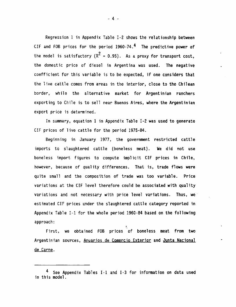
Regression 1 in Appendix Table I-2 shows the relationship between
CIF and FOB prices for the period 1960-74.4 The predictive power of
the model is satisfactory (R2 = 0.95). As a proxy for transport cost,
the domestic price of diesel in Argentina was used. The negative
coefficient for this variable is to be expected, if one considers that
the live cattle comes from areas in the interior, close to the Chilean
border, while the alternative market for Argentinian ranchers
exporting to Chile is to sell near Buenos Aires, where the Argentinian
export price is determined.
In summary, equation 1 in Appendix Table I-2 was used to generate
CIF prices of live cattle for the period 1975-84.
Beginning in January 1977, the government restricted cattle
imports to slaughtered cattle (boneless meat). We did not use
boneless import figures to compute implicit CIF prices in Chile,
however, because of quality differences. That is, trade flows were
quite small and the composition of trade was too variable. Price
variations at the CIF level therefore could be associated with quality
variations and not necessary with price level variations. Thus, we
estimated CIF prices under the slaughtered cattle category reported in
Appendix Table I-1 for the whole period 1960-84 based on the following
approach:
First, we obtained FOB prices of boneless meat from two
Argentinian sources, Anuarios de Comercio Exterior and Junta Nacional
de Carne.
4 See Appendix Tables I-1 and I-3 for information on data usedin this model.

- 5 -
Second, using a cost structure for 1985, we converted those FOB
prices to CIF prices in Chile.5 Cost items considered included
transportation, insurance, financial cost associated with the
operation, commission of the custom agent in Chile, and sanitary
inspection. The cost structure for 1985 was reconstructed for the
period 1960-84 using oil price variations for the transportation items
and a rate of interest of LIBOR plus 6 percent yearly for financial
costs. We also assumed that the ad valorem costs remained constant
at the 1985 level during the period under analysis. These criteria
were checked with current and previous meat importers. This, in
general, validated our procedure for estimating the cost structure.
Because transportation of this kind of processed beef is usually
agreed up to the final destination, CIF prices of boneless meat
reported in Appendix Table I-1 are those of the product placed in
Santiago, the major Chilean consumption center.
For milk, figures correspond to nominal dollars per ton of
powdered milk imported each year.6 The sources of information are the
same as those for wheat above. An alternative source of information
is FAO's Trade Yearbook. Its data are consistent with the figures
used in this study.
Available information does not allow us to estimate CIF prices of
imported milk according to the fat content in the powdered milk. The
Central Bank of Chile started classifying the product according to
this criterion only in 1979. But the Servicio Nacional de Salud
5 See Panorama Econ6mico de la Agricultura (DEA-UC) 41 and 42for details of this cost structure.
6 These figures do not include concessionary imports.

- 6 -
(SNS), the largest milk importer, has changed its import requirements
with regard to fat content. Up to 1976, SNS imported mostly low-fat
milk (12-18 percent). Around that year, and as a result of studies
showing caloric deficit in the target population, public sector
imports might have changed in favor of high-fat-content milk (26
percent). However, it was not possible to reconstruct a time series
for the 1960-84 period indicating the evolution of milk imports
according to the fat content.
Because changes in fat content of imported milk might induce
erratic changes in CIF average prices of powdered milk, some models
were designed to check whether the changes in these prices were
related to changes in FOB prices of the main exporters (Holland and
New Zealand). The assumption is that FOB average prices in the
exporter countries were not significantly affected by changes in
quality.
Results of these exercises are reported in Regressions 2, 3, and
4 of Appendix Table I-2. The high R2 in Regression 2 (0.83) shows a
strong correlation between CIF and FOB prices of powdered milk. A
problem with this model is that the high R2 could be just an
indication that both the CIF price of milk in Chile and the FOB price
of milk in New Zealand and Holland have a common trend pattern. In
addition, the low value of the Durbin-Watson test might indicate that
a relevant variable (such as fat content) was excluded from the
model. To cope with this problem, we performed a second test,
regressing a model in which the trend pattern was eliminated from the
variables by a polynomial adjustment. These results are reported in
equations 3 and 4. The R2 dropped to 0.24 to 0.28, and the FOB price
- 7 -
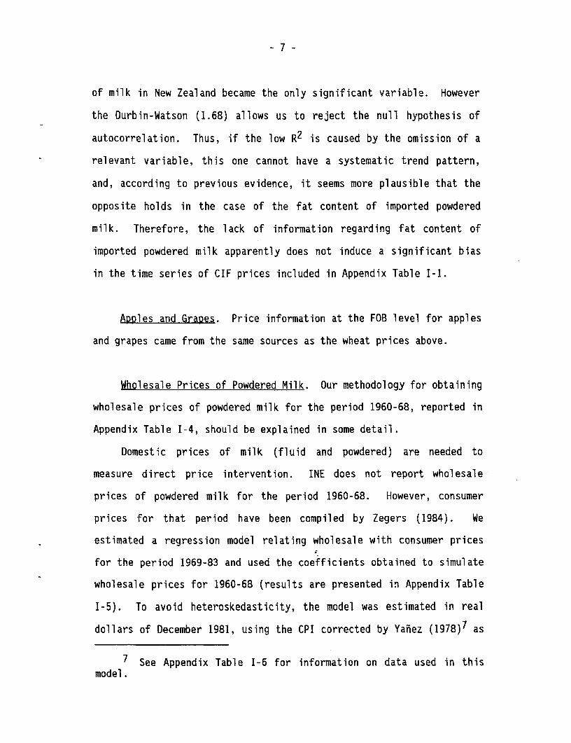
of milk in New Zealand became the only significant variable. However
the Durbin-Watson (1.68) allows us to reject the null hypothesis of
autocorrelation. Thus, if the low R2 is caused by the omission of a
relevant variable, this one cannot have a systematic trend pattern,
and, according to previous evidence, it seems more plausible that the
opposite holds in the case of the fat content of imported powdered
milk. Therefore, the lack of information regarding fat content of
imported powdered milk apparently does not induce a significant bias
in the time series of CIF prices included in Appendix Table I-1.
Apples and Grapes. Price information at the FOB level for apples
and grapes came from the same sources as the wheat prices above.
Wholesale Prices of Powdered Milk. Our methodology for obtaining
wholesale prices of powdered milk for the period 1960-68, reported in
Appendix Table I-4, should be explained in some detail.
Domestic prices of milk (fluid and powdered) are needed to
measure direct price intervention. INE does not report wholesale
prices of powdered milk for the period 1960-68. However, consumer
prices for that period have been compiled by Zegers (1984). We
estimated a regression model relating wholesale with consumer prices
for the period 1969-83 and used the coefficients obtained to simulate
wholesale prices for 1960-68 (results are presented in Appendix Table
I-5). To avoid heteroskedasticity, the model was estimated in real
dollars of December 1981, using the CPI corrected by Yanez (1978)7 as
7 See Appendix Table I-6 for information on data used in thismodel.

- 8 -
deflactor. The high R2 indicates the strong relation between the two
variables.
Prices for the period 1960-68 were obtained with the following
equation:
WPpm = 18.26 + 0.769 CPpm (A.1)
Nominal wholesale prices reported in Appendix Table I-6 for 1960-
68 were obtained by multiplying WPpm nominal by the Yaniez (1978)
adjusted Consumer Price Index, and where CPpm represents the consumer
price of powdered milk.
METHODOLOGY ON MEASURING DIRECT PRICE INTERVENTION
The figures reported in Table 3-2 in the text correspond to the
ratios between the adjusted border prices that would have prevailed
under free trade and the prices that effectively prevailed under the
"distorted" situation, at the official exchange rate. In general,
border prices reported in Appendix Table I-1 must be adjusted before
we compare them with the prevailing ("distorted") prices reported in
Appendix Table I-4, to measure properly the direct price
intervention. These adjustments are discussed now.
Wheat Adiustments. Three types of adjustments were made for
wheat. The first was for domestic transportation and custom
expenses. Because wholesale prices are measured in Santiago, and
import prices reflect CIF prices at the port of San Antonio (main port
of entrance for wheat), the CIF prices must be adjusted to make them

- 9 -
comparable to the wholesale prices at Santiago's level. These cost
adjustments include customs duties, unloading, transport cost from San
Antonio to Santiago, product losses in the process, and fees of the
custom agent. The breakdown of this cost structure was available for
1976, in Hurtado and Irarrazaval (1976).
To reconstruct the cost structure for the whole period 1960-84,
we used the following criteria. First, cost items that are
calculated as a proportion of the CIF values were considered constant
for the period. Second, cost items expressed in U.S. dollars were
supposed to remain fixed in real dollars for the whole period. Third,
unloading expenses (mainly labor) were assumed to vary with the wage
index calculated by INE for the period under study. Last, domestic
transportation expenses were assumed to vary according to the price of
domestic oil (at the wholesale level) also reported by INE. Following
this procedure, we estimated a cost structure for custom expenses and
domestic transportation for 1960-84.
The second adjustment for wheat was for quality. It is well
known that imported wheat is not perfectly comparable in quality with
domestic wheat. But what adjustment must be made to price of
imported wheat to make it comparable with domestic grain? Using
unpublished information generated by Fiscalia Nacional Econ6mica
(1981) and COPAGRO (1985), we developed a methodology to estimate the
magnitude of the required adjustment based on the following
assumption: (1) the current composition of wheat imports corresponds
70 percent to hard wheat and 30 percent to soft. (2) These
percentages have remained constant during the period 1960-84. (3) The
quality of domestically produced bread has remained constant during

- 10 -
the period 1960-84, in the sense that it is made of flour containing
fixed proportions of hard and soft wheat (52 and 48 percent,
respectively). (4) The average price difference at the FOB level
between hard and soft wheat was 10.3 percent (based on historical
evidence for the period 1976-84), and this difference remained
constant during the 1960-84 period. We thus posited the following
price relations between domestic wheat (Pa) and imported wheat (Pa'):
Pa' (0.7) (1.103) Pa'(S) + (0.3) Pa'(S)(A.2)
Pa (B) (1.103) Pa'(S) + (1-B) Pa'(S)
where:
Pa'(S) = International price of soft wheat, per unit. By
Assumption 4, Pa'(S) = Pa'(H)/1.103, where Pa'(H) is
the international price of hard wheat, per unit.
B = Hard wheat produced domestically as a percent of total
production. This coefficient was estimated using
Assumption 3, i.e.: 1 (0.7) + (1-y) (B) = 0.52, where -
represents annual imports as a fraction of consumption.
Using the above relationship the ratio Pa'/Pa was estimated for
the periods 1960-64 and 1971-84. The period 1965-70 was not estimated
directly and it was assumed to represefnt a transition phase for the
ratio Pa'/Pa. Quality adjustments for each period were made using the
following relationship:
Pa = 0.98 Pa', for 1960-64 (A.3)
= 0.97 Pa', for 1965-70 (A.4)
= 0.96 Pa', for 1971-84 (A.5)

- 11 -
Changes in quality (deterioration over time) of domestically
produced wheat are caused by locational factors of wheat production.
Specifically, the northern region of the country, producing mostly
hard wheat, has decreased its participation in total domestic
production during the period analyzed.
Compared with previous estimates of quality differences from
other sources, the estimated price differential for wheat that can be
explained by quality difference (hard vs. soft) in Chile is very small
-- from 2 to 4 percent in this study, compared with figures between 10
and 15 percent usually used in the country to reflect price
differences. Our interpretation of this discrepancy is that other
estimates have mixed quality differences with adjustments for
seasonality.
Regarding adjustments for seasonality, from the resource
allocation point of view, relevant producer prices are those
prevailing during the harvest period, because most farmers sell their
crop immediately after the harvest. Because of this, two domestic
wholesale prices are reported in Appendix Table I-4. These correspond
to the harvest period (January-July) and to the annual average price.
To measure direct price intervention, we must adjust border
prices not only for quality but for domestic transportation,
unloading and custom costs, and the costs of storage intrinsic to a
market in which demand is more or less constant over time but harvests
are concentrated during a couple of months. This storage process will
induce lower prices during the harvest season, even though free trade
prevails.

- 12 -
Storage cost has two components -- a direct cost derived from
the storage itself, which includes product losses, and a financial
cost, derived from the opportunity cost of the capital involved in the
process. If both components are taken into account, in equilibrium
the price seasonality must be such as to leave middlemen (farmers)
indifferent between buying (selling) during the harvest period or
later.
Calling Pa' the average border price of wheat in a certain year,
r the relevant discount rate including both financial and real cost of
storage, and T the month in which domestic consumption exceeds
domestic supply, then the average adjusted border price, APa', during
the sales period (January-July) can be calculated as:
APa' = [ Pa'/(1+r)T + ..... + Pa'/(l+r)T6 ] / 7 (A.6)
(l+r)7 - 1- Pa' ( ] / 7; T > 7 (A.7)
(1+r)T *r
In this framework, the discount rate, r, includes the relevant
rate of interest plus a 1-percent (real) cost per month, the latter
intended to account for the nonfinancial cost of storage.
With regard to the discount rate, we used two alternative rates.
One represents the prevailing nominal domestic interest rate, the
other represents an international rate of interest of LIBOR plus 6
percent annually, which reflects country risk and intermediation
spread. Our assumption is that given a distorted domestic rate of
interest, in the absence of intervention on capital flows it would be
reasonable to assume that domestic interest rates would vary according

- 13 -
to international rates adjusted by other specific country costs.
When domestic nominal interest rates were used as discount rates
for calculating APa', Pa' was converted from domestic currency to
U.S. dollars using the nominal exchange rate of month T. This
behavior implies that economic agents are able to predict Pa', the
average CIF price during the importing season, but not the exact
prevailing CIF price at month T. It also implies that economic agents
are able to predict perfectly the exchange rate at month T. This last
assumption, apparently asymmetric with the previous one, might sound
too restrictive for a particular year but not for the whole period.
This is defendable if we consider that the effect of "expected
devaluation" will be larger, the larger the overvaluation of the local
currency. But these periods correspond to years during which
economic agents (especially those related to international trade, such
as wheat millers) incorporate their expectations of exchange rate
variations with more emphasis in their economic transactions.
Pa' was obtained from the CIF prices of wheat reported in
Appendix Table I-1, previously adjusted by domestic transportation,
custom expenses and quality factors, described earlier. The ratios
between adjusted border prices (domestic transport cost, custom
expenses, quality, and seasonality) and relevant domestic prices
reported in Appendix Table I-4 are found in Table 3-2 in the text.
Basic information on domestic and international interest rates,
exchange rates, and T are reported in Appendix Table I-7.
Milk Adjustments. Ideally, border prices of powdered milk should
be adjusted by domestic transportation and custom expenses, quality

- 14 -
factors, and seasonality.
Because we lacked information on quality adjustments, we could
not reconstruct time series of imported milk classified by fat
content. In fact, there is no reliable information on this
variable. We have noted, however, that indirect evidence relates CIF
prices in Chile with FOB prices of powdered milk in the suppliers'
countries, showing that the quality factor (fat content) does not
induce too much variation in CIF prices. Still, this evidence is
obviously incomplete.
Regarding domestic transportation and customs expenses, most
powdered milk enters Chile through Valparaiso. Because wholesale
prices are reported in Santiago (the same as with wheat), we must
convert CIF prices into wholesale-equivalent prices in Santiago.
A cost structure for each year of the 1960-84 period is not
available. But fragmentary information indicates that customs-related
expenses are generally estimated as 3 percent of the CIF price. This
percentage has been stable over time. Domestic transport cost
estimates from Valparaiso to Santiago were available for 1984.
Therefore, the cost structure for the period 1960-84 was
reconstructed assuming that custom expenses remained constant over
time (3 percent over CIF) and that domestic transport cost (U.S.$
30/ton in 1984) varied for the period 1960-83 with the domestic oil
price.
Domestic prices reported in Appendix Table I-4 correspond to
annual averages for powdered milk. Seasonality adjustment were not
made in this case because processing plants do not store powdered
milk for long periods. Apparently, this is the result of a

- 15 -
countercyclical purchasing scheme of SNS, the principal buyer of
powdered milk in Chile.
Direct price intervention in milk can be estimated through two
alternative mechanisms. The first is to obtain the intervention by
comparing wholesale prices of powdered milk with the adjusted border
prices for this product and assuming that this percentage is fully and
quickly transmitted to producer prices of fluid milk. This
alternative is reported in Table 3-2 in the powdered milk column.
The second alternative for measuring direct price intervention in
milk is to estimated the price of fluid milk that would prevail under
free trade of powdered milk and then to compare it with prices of
fluid milk actually paid to domestic producers. It is clear that
domestic producers of milk react essentially to prices of fluid milk,
a nontradable product. Assuming that a percentage change in the
price of powdered milk is fully transmitted to the price of fluid
milk, as a result of the existence of a technological conversion
factor, clearly has a technical basis. But it oversimplifies the
economic relationships. Given the importance of milk production for
Chilean agriculture (see Hurtado, 1977), we devised a more
comprehensive approach.
Essentially, we sought a model that effectively relates wholesale
prices of powdered milk (WPpm) with the price of fluid milk paid to
producers (PPf). Once this relation was econometrically established,
simulations could be done to obtain prices of fluid milk under the
assumption of free trade in powdered milk. By definition,
PPf = a PPf(X) + (1- a) PPf(S) (A.8)

- 16 -
where
= Reception of milk by southern parts of Region IX, as a
proportion of total country reception
PPf = Weighted average of real producer prices of fluid milk
PPf(X) = Real price of fluid milk paid to producers in Region X
PPf(S) = Real price of fluid milk paid to producers in Santiago.
It is postulated that at the processing plant level, the
following relationships must hold:
WPpm(S) = al + bl PPf(S) or equivalently (A.9)
PPf(S) ab + bi WPpm(S) and (A.10)
WPpm(X) = a2 + b2 PPf(X) (A.11)
where:
WPpm(X) = Domestic wholesale price of powdered milk in Region X
WPpm(S) = Domestic wholesale price of powdered milk in Santiago
Given that the southern region; of the country (Region X)
"exports" powdered milk to Santiago (the consumption center), the
following arbitrage should hold:
WPpm(S) = cl WPpm(X) + c2 TC (A.12)

- 17 -
where:
TC = Domestic wholesale oil price, used as a proxy for
transportation cost between Santiago and Region X.
Replacing Equation (A.11) into Equation (A.12) and reordering
terms, PPf(X) can be rewritten as:
PPf(X) = 2 - C2 TC + I WPpm(S) (A.13)b2 clb2 cIb2
Replacing Equations (A.13) and (A.10) into (A.8), PPf can be
expressed as a function of WPp(S), that is:
ppf l + a l a 2 )a(A.14)
+ - 1 a WPpm(S)clb2 bl
+ 1b WPpm(S) -c2 a TCbl ~~clb2
Finally, Equation (A.12), expressing the average producer price
of fluid milk as a function of the wholesale prices of powdered milk
in Santiago, was estimated econometrically as:
PPf = dO + dl a + d2 a WPpm(S) + d3 a TC + d4 WPpm(S) (A.15)
where the expected signs of the regression coefficients - d - are:
dO = Al bi <°, d3 = c-b2 < O , d4 I > Lbl ~~~clb2 -bl>

- 18 -
while dl and d2 have undefined sign, a priori.
The model reported in Equation vii was estimated for the 1960-84
period. The results are reported in Regressions 2 and 3 of Appendix
Table I-8. Both regressions exhibit high values for R2 and the
expected signs for the coefficients, except for the transportation
variable, a - TC, which is not statistically significant.
Furthermore, dl (the coefficient associated with variable a) is
positive, indicating that when this variable increases, PPf also
increases.8
Because of autocorrelation problems in Regression 2, the
regression coefficients associated with Regression 3 were used in the
subsequent analysis.
Initially, we thought that the model reported in Regression 3,
Appendix Table I-8, could be used to simulate the level of producer
prices of fluid milk, assuming free trade of powdered milk. However,
when we followed this procedure, producer prices of fluid milk in
some years became negative. This outcome, in our opinion, was the
result of the high level of protection enjoyed by the production of
powdered milk during the period analyzed (see column 5 Table 3-5).
Under free trade, domestic prices of powdered milk would decrease
substantially, inducing a significant decrease in producer prices of
fluid milk. Such a large extrapolation with this model does not seem
reasonable from an economic point of view, considering that some
regional readjustments could occur, and this model does not allow for
this possibility.
8 The dynamics of this process will be discussed later, when ais endogenized in the model.

- 19 -
Considering the magnitude of the change in producer prices
induced by free trade in powdered milk, it seems too restrictive to
assume that a (the percentage of milk production at the south of
Region IX) remains constant during the period of analysis. The
presumption is that the values of a that prevailed under closed
economy conditions would change under free trade. From an economic
and agronomic point of view this is consistent given that the southern
regions of the country have comparative advantage for producing milk,
and, therefore, one would expect a to increase in response to lower
producer prices of fluid milk.
The above considerations imply that the assumption of a constant
a should be relaxed. The analysis thus should attempt to explain its
variability as a function of variables that in turn would be affected
by a trade liberalization.
We assumed that a should depend on the relative profitability (R)
of other agricultural activities that compete with milk production in
the use of land. If these competing activities became more
profitable, we would expect milk producers located in the more
inefficient regions (central valley) emigrate to the South, to benefit
from the cost advantages of producing milk there or to stop producing
milk and reallocate their resources to more profitable uses. These
options are wider in the central valley of Chile.
However, a should depend not only on current values of R but
also, and perhaps more importantly, on producers' expectations for
future values of R.
Assuming that at depends on the expected value of R at time t,*Rt, and the existence of an adaptive expectations adjustment mechanism.

- 20 -
of the following type:
Rt- Rt 1 = (Rt -Rt-1) (A.16)
where:
0 < - < 1,
a reduced form equation is obtained:
at = eO + el Rt + e2 at-, (A.17)
where the short-run adjustment of at with respect to changes in Rt is
given by the coefficient el, and the long run adjustment is given by
el/(1-e2).
Equation (A.17) was estimated for the period 1960-84 using as a
proxy of Rt the ratio between the wholesale price of powdered milk in
Santiago and the FOB price of grapes, converted to local currency at
the official exchange rate. The export price of grapes was included
as a proxy intended to capture the effect of nontraditional options
for land use in the Chile's central valley. The estimated equation is
reported in Regression 1, Appendix Table I-8. The adjusted R2 is
reasonably high (0.79), and the signs of the coefficients are as
expected.
Short- and long-run elasticities of a with respect to R could be
used to simulate the value of a under free trade conditions a . There
were at least two options to proceed. First, we could use both
elasticities and a dynamic approach. The problem with this method is
the high sensibility of results with respect to the initial value of
a. Second, we could use the long-run elasticities to adjust the

- 21 -
values of a with respect to changes in R. This method induces drastic
changes in as from year to year that do not seem reasonable
considering producers' historical response to changes in relative
prices. Therefore, we used short-run elasticities to simulate a*. In
our opinion, these parameters reflect more adequately farmers behavior
with regard to price changes.
Actual values of a and the simulated ones are reported in
Appendix Table I-9. These simulated values were used together with
the coefficients of Regression 2 of Appendix Table I-8 to estimate
producer prices of fluid milk under free trade and, therefore, direct
price intervention. It must be emphasized that the geographic
adjustment allowed by variations in a decreases the decline in
producer prices of fluid milk resulting from reductions in prices of
powdered milk as a result of trade liberalization. Increases in a
imply, all other things being equal, increases in the price of fluid
milk paid to producers (see Regressions 2 and 3, Appendix Table I-8).
However, even with this geographic adjustment, producer prices of
fluid milk continued to be negative for the period 1960-63.
Finally, some limitations of the above procedure should be
emphasized. If a depends on other variables, Equation vii should be
estimated using a two-stage least square and not directly, as done in
Regressions 2 and 3 of Appendix Table I-8.
This option was not taken because of the following reasons.
First, even if a is endogenous, for a given year it can be considered
predetermined, because geographical adjustment is not instantaneous.
Second, from an empirical point of view, the two-stage estimation
generated a problem of multicolinearity, which is responsible for

- 22 -
coefficients that are not statistically significant. Because these
coefficients were needed to measure direct price intervention, the
approach was not feasible. For illustration purposes only, Regression
4 of Appendix Table I-8 reports the results of the two-stage least
square estimation.
Cattle Adjustments. As indicated at the outset of this Chapter,
direct price intervention in cattle was estimated under two different
scenarios: one of no restrictions on international trade for live
cattle and another of trade only in boneless meat. Given that
sanitary restrictions to prevent hoof-and-mouth disease were included
in the cost structure of the first scenario, both scenarios are
consistent with disease prevention.
The basic information to simulate the price of imported live
cattle under free trade conditions are the CIF prices reported in
Appendix Table I-1. These prices must be adjusted to make them
comparable to the wholesale domestic prices and to estimate direct
price intervention.
The relevant cost structure was available for 1985 and was
discussed with meat importers to reconstruct it for the 1960-84
period. Fortunately, cost items were generally charged as a
percentage of a basic price. The adjustments to convert CIF prices of
live cattle into ex-customs prices in Los Andes (the point of entrance
for the majority of imports during the period under study) were as
follows. (1) There were bank fees for the operation (2.5 percent over
the CIF price). (2) Financial cost was included (90 days at a rate of
LIBOR plus 6 percent annually, estimated over the CIF price increased

- 23 -
by bank fees). (3) Customs agent costs (1 percent over the CIF price
adjusted by bank and financial costs. (4) Sanitary inspection (U.S.$
2.67 per ton, considered constant in real dollars for the period) was
also considered.
The CIF price adjusted by Items 1 to 4, converted to local
currency at the official exchange rate, corresponds to the price of
imported live cattle in Los Andes. This price must be adjusted by a
fifth factor (5), domestic sanitary regulations (cuarentena),
consisting of 30 days of isolated feed-lot quarantine. This item was
estimated according to the feed requirement (essentially alfalfa hay)
and varied for the 1960-84 period according to the domestic wholesale
price of alfalfa's hay. (6) There was an adjustment for domestic
transportation from Los Andes to Santiago ($3 per kg. in 1985,
estimated for the 1960-84 period according to the evolution of
domestic wholesale price of oil). Finally (7), there was a profit
margin for the importer (25 percent of the CIF price increased in
Items 1 to 6).
The profit margin of Item 7 above was included to reflect the
institutional operation of this market. Most of meat imports were
done by private agents who normally sell the product to wholesalers.
Therefore, the importer's margin is an item that must be considered in
the border price adjustments for measuring direct price intervention.
Appendix Table I-7 reports basic information were used to perform
these adjustments.
Imports of slaughtered cattle have a cost structure that includes
all expenses up to the moment the product is placed in Santiago.
However, the relevant arbitrage mechanisms needed to estimate direct

- 24 -
price intervention are related to the producer price of live cattle.
Therefore, prices of imported slaughtered cattle must be converted
into their equivalent in terms of live cattle. This transformation is
not simple, because it includes technical and economic
considerations. We had to convert prices of boneless imported meat
into equivalent carcass price (i.e., slaughtered cattle with bones).
This was carried out by the following relationship.9
Pm = Pc- Pmb (A.18)-7
where:
Pm = Price of imported boneless meat, in Santiago
Pc = Domestic price of carcass
Pmb = Domestic price of meat with bones
-Y = Conversion factor indicating the proportion of boneless
meat within the carcass weight.
In this context, the above relationship determines the maximum
domestic carcass price that is consistent with Pm and Pmb, where Pm
is exogenous for the country, predetermined by the international
market.
Once Pc has been estimated, for each year, the problem is to
simulate the domestic price of live cattle that would have existed if
P2 prevailed. For that purpose the following relationship was used:
Plc = Pc + VP - SC (A.19)
where:
VP = Domestic value of byproducts generated by the slaughtering
9 See Panorama Econ6mico de la Agricultura (DEA-UC) N 41 and42, for more details.

- 25 -
process (mainly skins and grease)
SC = Domestic cost of the slaughtering process to the producer
Plc = Domestic price of live cattle.
It must be emphasized the nature of Plc so obtained, because it
predetermines the economic interpretation that should be given to the
direct price intervention reported in the relevant tables and also to
the subsequent indicators that use direct intervention as an input
(indirect price intervention, effective protection rate, etc.). To
clarify this important aspect, we present the following illustration.
Figure I-1 The Beef Market in Chile: A Typical Scenario
p
Plc
plcnt X*X
Plc* X
D
Q
Historically, meat imports in Chile have represented a small
fraction of domestic consumption, except for a few years. Imports of
live cattle were permitted up to 1975. Under a free trade situation,
this scenario would have been consistent with a domestic price of

- 26 -
Plc*. However, because sanitary regulations (cuarentena) were
typically evaded and because the government usually intervened as an
importer of meat and often without operating with a competitive
margin, domestic prices were usually below Plc*, for example, Plct.
Under these conditions, the ratio Plc*/Plct is an appropriate
measurement of direct price intervention, as reported in Table 3-1.
From 1976 on, sanitary regulations were drastically modified, and
live cattle imports were forbidden. Under these conditions, the CIF
price of slaughtered cattle imposed a maximum domestic price of Plc
for live cattle. However, it would seem that for many years after
1975, domestic prices of meat were not affected significantly by Plc
(except for a few months during which domestic supply falls because of
seasonal factors). The implication of this is that the domestic meat
market has behaved as a nontradable market, with an equilibrium price
of Plcnt. Hence, measuring direct price intervention as Plc/Plcnt may
be misleading for some years.10 Therefore, the value for direct
intervention was made equal to 1.0 for years in which beef was not
protected (i.e., after 1975). Again, the implications of the above
discussion are important to interpret the measures of direct price
for live and for slaughtered cattle price intervention reported in
Table 3-2.
Apples and Grapes. Prices of apples and grapes at the FOB level
must be adjusted to estimate direct price intervention in a
10 The analysis assumes that the relevant FOB price faced byChilean meat producers is below Plct, which is based on empiricalevidence.

- 27 -
meaningful way. These adjustments are of three types: quality
adjustments, export subsidies, and exchange rate adjustments.
Domestic prices of apples and grapes cannot be used to estimate
direct price intervention, because normally the nonexported fraction
of these fruits is of inferior quality to the exported one. We solved
this problem by estimating directly the domestic price of the
exported fraction (FOB prices at the packing-house level). The
adjustments required to convert FOB prices at the country level to FOB
prices at the packing level included domestic transportation, exporter
commissions, packing materials and handling, and other services.
The export subsidies were legislated as a percentage of the FOB
price. Therefore, this subsidy must be incorporated at the FOB
packing level, for purposes of estimating direct price intervention.
Finally, during 1963-65 and 1972-73, the exchange rate for
agricultural exports was higher than for nonagricultural exports.
Expressing the agricultural exchange rate as a percentage of the
general exchange rate, the subsidy for agricultural exports was
significant (18 percent, 10 percent, and 6 percent) for 1963, 1964,
and 1965, respectively. It was 12 percent and 15 percent for 1972 and
1973, respectively (see Hachette and De la Cuadra, 1984, Appendix p.
18). Therefore, these exchange rate subsidies were included when we
converted FOB prices in local currency and when we estimated farmgate
prices (FOB packing) of the tradable fraction of apples and grapes.
Direct price intervention in apples and grapes was estimated
adjusting the border prices reported in Appendix Table I-1 according
the quality, export subsidy, and exchange rate adjustments noted
above.

- 28 -
A complete explanation of each of the adjustments is given in
the footnotes of Appendix Table I-1. Information on export subsidies
and exchange rate subsidies for fruit exports (this applies only to
1962-74) are reported in Appendix Table I-10.

- 29 -
Table I-1 Border Prices (PA)
Slaugh-tered Live Powdered
Year Wheat Cattle Cattle Milk Apples Grapes
(US$/ton)
1960 62.9 662.2 291.7 372.8 93 1561961 71.4 610.8 274.4 296.3 119 2001962 78.4 538.5 241.7 361.0 117 1981963 71.8 531.7 221.6 301.6 115 1761964 81.6 619.6 396.9 255.3 130 1601965 66.9 1037.1 419.9 387.3 120 1701966 49.2 1121.9 428.3 430.2 128 1781967 73.6 1078.1 385.1 400.2 129 1961968 70.3 839.8 395.4 332.2 129 2121969 77.4 840.3 392.7 290.4 154 2271970 72.4 965.0 421.4 463.8 184 2541971 70.3 1429.7 560.4 605.8 172 2591972 72.5 1570.4 703.9 796.8 210 2801973 154.2 2221.2 736.8 658.4 262 3131974 204.9 2320.9 815.7 679.4 189 3371975 192.5 1709.4 567.5 800.0 339 5361976 239.5 1483.5 361.0 667.0 247 4961977 115.7 1542.8 560.8 757.6 257 5241978 140.8 1570.4 429.3 877.5 364 6411979 188.0 2868.7 717.1 995.0 346 8821980 202.0 3283.2 792.2 1316.0 458 8771981 205.0 3502.3 846.3 1487.0 435 9531982 177.0 2700.8 886.0 1417.0 450 9861983 171.0 2654.2 770.1 1340.0 351 8391984 161.0 1701.3 368.8 1062.0 367 923
Source: Authors calculation - See Appendix I for details.

TABLE 1-2 Relationship Between C.I.F. and F.O.B. Prices in Cattle and Milk
Regression Period Dependent Independent Variables R F DW
Covered Variable Constant LN(ARlc) LN(SAoil) LN(HOpm) LN(NZpm) LN(OF) LN(ARtc)
1 1960-74 LN(CHlc) -1.92 1.09 -0.34 0.95 117.9 2.07
excl.1962 (11.5) (-3.08)
annual
2 1960-81 LN(CHpm) 0.40 0.48 0.46 0.68x10 0.83 34.5 0.79
annual (2.11) (2.25) (0.00)
3ji 1960-83 LN(CHpm) 0.00 -4.48 0.16 0.350 0.24 3.4 1.68
annual (-0.45) (0.80) (2.02)
41/ 1960-83 LN(CHpm) 0.00 0.380 0.28 10.0 1.68
annual (3.16)
1/ The trend pattern has been eliminated in all variables of the regression.
LN = natural log operator CHlc = c.i.f. price of live cattle, Chile US$/tonARsc = c.i.f. price of slaughtered cattle ("cuartos") Argentina, US$/tonSAoil = f.o.b. price of oil, South Arabia," US$/barrel
HOpm = f.o.b. price of powdered milk, Holland, US$/ton
NZpn = f.o.b. price of powdered milk, New ZealandOF = ocean freight for grains shipments from Argentina to Holland (Rotterdam), US$/ton
CHpm = c.i.f. price of powdered milk, Chile, US$/ton
ARtc = price of Argentinean Diesel, US$/Lt.
Data Source Tables 1-1 and 1-3.

- 31 -
Table I-3 Data Used for Estimating Border Price of Cattle andFat Content Analysis of Milk
Slaughtered OilCattle FOB Price ofFOB Powdered Milk FOB Saudi Diesel
Argentina Holland New Zealand Arabia Argentina
(US$/ton) (US$/ton) (US$/ton) (US$/ (US$/lt)barrel)
1960 442.8 524.3 250.3 1.87 0.061961 403.0 574.5 225.4 1.80 0.061962 na 533.3 201.8 1.80 0.051963 378.5 525.8 199.2 1.80 0.051964 513.7 548.6 205.6 1.80 0.051965 617.3 454.4 298.3 1.80 0.061966 561.8 443.5 301.9 1.80 0.061967 470.9 493.3 299.8 1.80 0.051968 520.6 400.3 241.1 1.80 0.051969 513.1 469.5 191.7 1.80 0.051970 582.2 478.4 188.9 1.80 0.041971 804.4 636.6 237.5 2.19 0.061972 959.9 726.9 470.5 2.38 0.061973 1375.7 784.2 549.1 3.28 0.121974 1387.8 943.8 669.9 11.58 0.151975 882.6 1283.6 877.4 10.72 0.081976 621.7 1139.9 611.4 11.51 0.101977 934.3 1203.0 436.5 12.40 0.101978 864.5 1381.8 537.6 12.70 0.181979 1474.9 1125.8 664.8 16.97 0.221980 1775.5 1522.8 785.3 28.67 0.301981 1931.6 1690.3 1106.7 32.50 0.321982 1632.1 1638.3 1239.5 33.47 0.161983 1512.6 1500.7 1087.1 29.31 0.191984 776.7 na na 28.47 0.20
SOURCES:Column 1: Anuarios de Comercio Exterior, Argentina for
1960-67 and Junta Nacional de Carnes, from1968 on.
Columns 2 and 3: FAO. Trade Yearbook.Column 4: IMF. IFS.Column 5: Sturzenegger (1985)

Table 1-4 Nominal Domestic Prices of Selected Agricultural Products (PA)
Wheat Beef Milk Apples Grapes
Annual Harvest Domestic Exportable Domestic ExportableAverage (Jan-Jul) Aug Live Slaughtered Fluid Powdered Quality Quality Quality Quality
($/100 kg.) (S/live ($/kg.) ($/1000 lts.) ($/kg.) ($/100 kg.) ($/100 kg.)ton)
1960 0.007703 0.007534 0.3568 0.00060 0.05976 0.001261 na 0.00399 na 0.00733
1961 0.007778 0.007631 0.3690 0.00063 0.06485 0.001280 0.01097 0.00615 0.00864 0.01098
1962 0.009010 0.008229 0.4132 0.00069 0.0792 0.001521 0.01666 0.00645 0.01069 0.0116
1963 0.01223 0.012094 0.6387 0.00106 0.10594 0.002140 0.02153 0.0147 0.0134 0.02271964 0.01803 0.017799 1.111 0.00175 0.1344 0.002723 0.03632 0.0196 0.0270 0.0206
1965 0.026 0.0257 1.449 0.00227 0.2095 0.003986 0.0393 0.0211 0.0310 0.02721966 0.034 0.033 1.800 0.00268 0.332 0.005005 0.0881 0.0253 0.0520 0.0225
1967 0.039 0.038 2.137 0.0033 0.408 0.005968 0.0929 0.0442 0.0587 0.06601968 0.049 0.048 2.747 0.0046 0.496 0.007841 0.1252 0.060 0.0717 0.1021
1969 0.067 0.065 3.979 0.0074 0.666 0.01078 0.f873 0.102 0.1087 0.1464
1970 0.088 0.085 5.705 0.0104 0.873 0.0138 0.295 0.161 0.1475 0.2095
1971 0.106 0.105 8.476 0.0125 1.126 0.0146 0.327 0.154 0.1518 0.201
1972 0.132 0.13 12.195 0.0229 1.451 0.0306 0.909 0.395 0.3760 0.416
1973 0.483 0.25 88.58 0.1230 13.48 0.15 4.27 2.538 na 3.104
1974 12.41 8.51 798.2 1.0692 97.82 1.75 19.38 9.188 na 21.09
1975 78.11 57.54 1437 2.750 423.1 7.89 82.1 113.5 36.9 190.061976 224.0 212.48 7357 12.84 1344 24.43 227.9 174.3 118.5 403.2
1977 375.9 365.83 17620 32.67 2611 42.52 571.0 284.5 360.2 682.1
1978 496.2 466.0 26880 46.17 4076 65.34 549.8 700.6 528.4 1301.9
1979 659.8 572.1 40610 68.83 5975 95.67 663.0 653.6 677.5 2134.9
1980 821.4 783.0 51800 92.17 7467 133.77 925.8 929.5 1034.5 1950.2
1981 911.5 916.6 49880 95.67 7005 137.70 921.4 739.1 1022.9 2025.8
1982 961.4 829.6 46520 92.83 8431 135.61 832.1 1116.5 693.0 2965.51983 1660.2 1458.9 57200 110.0 11647 209.96 1038.6 1177.3 714.7 3839.2
1984 2100.4 1940.0 83400 165.0 16298 293.06 1025.9 1610.3 986.8 5549.3

- 33
Notes:
The prices of fluid milk are a weighted average of the pricepaid by the Cooperativa Lechera de Santiago and plants in theRegion X of the country. The weights are the actual a'sreported in Table I-9.
2/ The domestic prices of apples and grapes are those at thewholesale level in the Mercado Central of Santiago. Annualaverages were calculated using monthly averages, weighted by thevolume marketed in each month. For 1966 the source did notprovide information on monthly volumes marketed, thereforemonthly prices were weighted using a seasonality indexconstructed by CORFO (1970) Precios de la Fruta en el MercadoInterno, for the period 1966-69. A similar approach was usedfor the period 1970-72, where weights were taken from aseasonality index elaborated by CORFO for the indicated period.
l/ Export prices of apples and grapes correspond to the domesticprice of the exported fruit, which differs from the domesticprices of the nonexported apples and grapes. The fraction soldinternally is, in general, of a different quality than theexported one. Therefore, for purposes of estimating theimplicit tariff needed to calculate direct price intervention inthese two products, domestic prices of the nonexported fractionreported in the Table cannot be used.
The domestic prices of the exported fruit were calculated asfollows:
(i) FOB prices in Chile were converted to FOB at the packinglevel by prices using a cost structure taken from PanoramaEconomico de la Fruticultura (1984). This structure,calculated for 1984, includes domestic transportation,exporter commissions, packing materials, handling and otherservices. This structure, for each fruit, wasreconstructed for the period 1960-83 using domestic pricesof oil, salaries and the wholesale price index to estimateprevious prices of domestic transportation, services andpacking materials, respectively. The exporter commissionwas assumed to be 10 percent of the FOB value, for thewhole period, based on experts' opinions.
(ii) During some years (see Table I-10 of the Appendix) therewas an export subsidy that, according to the law, was fixedas a percentage of the FOB value. This subsidy, whichvaried constantly during the analyzed period, wascalculated for each specie and variety as as weightedaverage of the volume exported in each period, specie andvariety. For 1973 the weights were not available toestimate the incidence of each variety within the totalexported in apples; interpolation for the period 1966-83was used instead. The information for 1966 was taken from

- 34
CORFO (1983) Plan Nacional de Desarrollo Fruticola, Vol.II, page 229 and for 1983 from Panorama Economico de laAgricultura N042.
In general, the subsidy, S(X), was calculated as
S(X) =- B P(DX)P(D)
where: B = percent of government devolution, on a FOBbasis in each specie and variety
P(X) = FOB price of each specie and varietyP(D) = domestic price of the exported fruit, at the
packing level
Therefore, domestic prices of the exported fraction ofapples and grapes were calculated adding the export subsidyS(X) to the farm gate (FOB packing) prices calculatedaccording to (i).
(iii) During some years (1963-65 and 1972-73), the exchange ratefor agricultural exports was higher than for nonagriculturalexports (see Hachette and de la Cuadra (1984)). Therefore,these exchange rate adjustments were considered to convertFOB prices in local currency and to estimate farm gateprices (FOB packing) of the tradable fraction of apples andgrapes. See Table I-10 for information on exchange rateadjustments.
The prices reported in the Table above, including adjustment for(i), (ii) and (iii) were used to estimate direct prices interventionin apples and grapes.
SOURCES:
Wheat, SlaughteredCattle, Powdered Milk: INE, wholesale prices. For 1960-68,
wholesale prices of powdered milk wereestimated specifically for this studysince they were not available. SeeAppendix for more information.
Live Cattle: 1960-74 Zegers (1984) Subsistema de Producci6nLechera;
1975-84 ODEPA Boletin Pecuario, various issues.
Fluid Milk: 1960-83 Zegers (1984) Subsistema de Producci6nLechera;
1984 Depto. Economia Agraria, U.C. Central deInformaciones, based on information givenby SOPROLE.

- 35
Domestic Apples andGrapes: 1961-65 CORFO (1968) Plan Nacional de Desarrollo
Fruticola, page 45;
1966 Ministerio de Agricultura (1967) Preciosde Productos Agropecuarios;
1967-72 CORFO (1976) and (1974) Precios de laFruta en el Mercado Interno;
1972-73 Not available;
1975-84 Depto. Economia Agraria, U.C., Central deInformaciones.
Exported Apples andGrapes: See notes above.

- 36 -
TABLE I-5 Relationship Between Wholesale and Consumer Prices of Powdered Milk
Period Dependent Independent Variabj eCovered Variable Constant Dummy CPpm2 Re F DW
1969-83 WPpm 18.26 -24.19 0.769 0.957 147.9 2.00annual (5.10) (14.28)
WPpm = domestic wholesale price of powdered milk, real $/kg., Dic. 1981.Dummy = dummy variable that takes the value 0 between 1969 and 1976 and 1, otherwise.
Included to incorporate the establishment of the value added tax, in 1977.CPpm2 = domestic consumer price of powdered milk, real $/kg., Dic. 1981.
Data Source: Table I-6
- 37 -
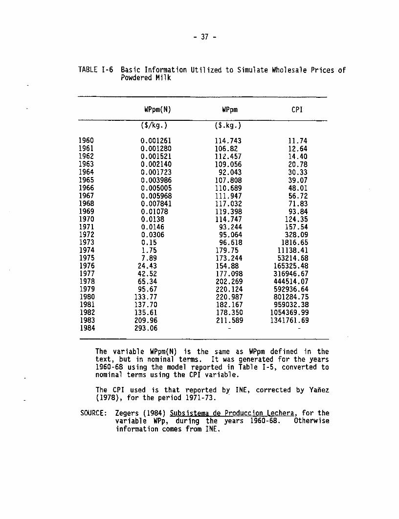
TABLE I-6 Basic Information Utilized to Simulate Wholesale Prices ofPowdered Milk
WPpm(N) WPpm CPI
($/kg.) ($.kg.)
1960 0.001261 114.743 11.741961 0.001280 106.82 12.641962 0.001521 112.457 14.401963 0.002140 109.056 20.781964 0.001723 92.043 30.331965 0.003986 107.808 39.071966 0.005005 110.689 48.011967 0.005968 111.947 56.721968 0.007841 117.032 71.831969 0.01078 119.398 93.841970 0.0138 114.747 124.351971 0.0146 93.244 157.541972 0.0306 95.064 328.091973 0.15 96.618 1816.651974 1.75 179.75 11138.411975 7.89 173.244 53214.681976 24.43 154.88 165325.481977 42.52 177.098 316946.671978 65.34 202.269 444514.071979 95.67 220.124 592936.641980 133.77 220.987 801284.751981 137.70 182.167 959032.381982 135.61 178.350 1054369.991983 209.96 211.589 1341761.691984 293.06 - -
The variable WPpm(N) is the same as WPpm defined in thetext, but in nominal terms. It was generated for the years1960-68 using the model reported in Table I-5, converted tonominal terms using the CPI variable.
The CPI used is that reported by INE, corrected by Yafiez(1978), for the period 1971-73.
SOURCE: Zegers (1984) Subsistema de Produccion Lechera, for thevariable WPp, during the years 1960-68. Otherwiseinformation comes from INE.

Table 1-7 Basic Information Utilized to Calculate Direct Interventions in Wheat, Cattle and Milk
FOB price of
Nominal Exchange rate Eo Wage Domestic Domestic Value Argentina's Interest Rates
Annual Jan-Jul Index Price Price of of Animal Slaughtered (monthly)
Year Average Average Month T T (Annual Average) of Oil Rib Meat Byproducts Cattle Domestic Libo
($/US$) ($/US$) ($/US$) ($/m3) ($.kg.) ($/kg.) (US$/ton)
1960 0.001051 0.001051 0.001051 11 0.00115 0.04367 0.000684 0.0455 442.8 1.29 0.80
1961 0.001051 0.001051 0.001051 11 0.00133 0.04367 0.000748 0.0483 403.0 1.57 0.79
1962 0.001142 0.001051 0.001051 9 0.00151 0.04525 0.000804 0.0528 na 1.12 0.80
1963 0.001875 0.001811 0.001906 9 0.00218 0.06452 0.001165 0.0824 378.5 1.12 0.80
1964 0.002372 0.002310 0.002446 10 0.00300 0.08407 0.001940 0.149 513.7 1.16 0.83
1965 0.003128 0.002973 0.003276 9 0.00443 0.10115 0.00254 0.199 617.3 1.21 0.87
1966 0.003955 0.003762 0.004096 8 0.00613 0.1199 0.00300 0.232 561.8 1.23 0.98
1967 0.005031 0.004730 0.005288 9 0.00833 0.1479 0.00330 0.249 470.9 1.23 0.93
1968 0.006787 0.006420 0.007154 9 0.01062 0.1964 0.00372 0.237 520.6 1.29 0.99
1969 0.008974 0.008457 0.009621 9 0.01503 0.2474 0.00400 0.301 513.1 1.47 1.23
1970 0.011552 0.01108 0.01221 10 0.02195 0.3494 0.00436 0.468 582.2 1.53 1.13
1971 0.012409 0.01221 0.01221 8 0.03315 0.3791 0.00488 0.684 804.4 1.17 1.01
1972 0.019485 0.0158 0.0158 7 0.05530 0.4709 0.00719 2.14 959.9 1.35 0.94
1973 0.110798 0.0368 0.025 4 0.161 4.886 0.04319 21.95 1375.7 2.82 1.19
1974 0.832 0.563 0.611 5 1.204 67.97 0.2973 102.5 1387.8 7.62 1.32
1975 4.91 3.491 5.339 7 5.606 494.8 0.955 322.2 882.6 14.56 1.07
1976 13.05 11.50 i2.56 5 23.55 1516 16.77 1427.7 621.7 13.36 0.96
1977 21.54 19.24 21.96 8 50.96 2372 42.5 2925.7 934.3 8.16 0.98
1978 31.67 30.45 31.30 5 81.38 3571 63.0 4572.4 864.5 5.28 1.18
1979 37.25 36.00 36.76 6 120.25 8152 86.87 6635.5 1474.9 4.10 1.40
1980 39.00 39.00 39.00 6 176.64 11766 117.41 6246.0 1775.5 3.25 1.55
1981 39.00 39.00 39.00 4 230.20 12260 125.7 3962.2 1931.6 3.54 1.72
1982 50.91 40.67 39.00 4 252.49 14260 128.5 3793.4 1632.1 4.16 1.49
1983 78.79 75.57 73.69 4 287.09 21631 147.7 8638.3 1512.6 3.03 1.24
1984 98.48 89.42 91.10 6 344.43 27469 198.7 16402 776.7 2.70 1.33
SOURCES:Columns 1, 2, 3, 10 and 11:Banco Central de Chile
Column 4: Copagro (1984)
Columns 5 and 6:INE
Column 7:INE. Since for 1975 there was no information on rib meat price, the annual variation of the roast beef was used as proxy.
Column 8:Corresponds to a weighted average of wholesale prices of cow skin and animal fat.
Column 9:Anuarios de Comercio Exterior, for the period 1960-67 and Junta Nacional de Carnes for 1968-84.

TABLE 1-8 Models Used to Estimate Nominal Rate of Protection on Fluid Milk
Regression Period Derendent Independent Variables RHO R F DW
Covered Variable Constant R at-1 aWPpm TC a WPpm
1 1960-84 a 0.544 -0.019 0.361 - - - - - 0.78 44.8 1.33
annual (6.45) (-2.38) (4.66)
2 1960-84 PPf -36954 - - -0.457 2.58 54717 0.370 - 0.81 27.6 2.62
annual (-2.44) (-2.28) (0.61) (2.61) (2.57)
3 1961-84 PPf (-42731) - _ -0.529 1.35 61681 0.43 0.397 0.83 29.6 2.22
annual (-2.88) (2.63) (0.36) (2.98) (2.99) (-2.12)
4 1961-84 PPf -15333 - - -0.11 -2.44 25798 0.12 - 0.79 23.6 2.30
annual (-0.92) (-0.51) (-0.45) (1.1) (0.75)
a = plant reception of mi'l'k south of region IX, as a proportion of total country reception.
PPf = weighted average of real producer prices of fluid milk, $/lt. December 1981, calculated as
PPf = aPPf(X) + (1-a) PPi`(S)
WPpm = domestic wholesale price of powd Ired milk, real $/kg., December 1981
TC domestic wholesale oil price, $Im , December 1981,
R = WPp/Pg
Pg = f.o.b. price of grapes, Chile, US$/ton, using the offical exchange rate to convert prices into domestic currency.
SOURCE: Tables 1-4 and 1-7.
NOTE: Regression 4 corresponds to a 2-stage estimation, where a is replaced by the estimator obtained with regression 1.

- 40 -
TABLE 1-9 Geographic Adjustment of Milk Producers Under Free TradeConditions
aYear Proportion Proportion
1960 0.47 0.571961 0.52 0.601962 0.50 0.591963 0.53 0.621964 0.59 0.691965 0.63 0.721966 0.65 0.731967 0.68 0.751968 0.70 0.761969 0.71 0.781970 0.68 0.721971 0.71 0.741972 0.73 0.771973 0.75 0.781974 0.75 0.821975 0.73 0.761976 0.75 0.791977 0.78 0.811978 0.77 0.801979 0.72 0.741980 0.76 0.801981 0.79 0.821982 0.78 0.801983 0.78 0.801984 0.75 0.78
a = plant reception of milk in regions IX and X as a proportion of totalcountry reception. a refers to actual and a* refers to theestimation of a under free trade conditions.
SOURCE: ODEPA, Boletin Agroestadistico de Leche (various issues), for aand Table I-8 regression 4, for a* values.

- 41 -
TABLE I-10 Exchange Rate and Export Subsidies on Apples and Grapes(1962-1974)
Year NERa/NER Sa Sg
19621963 181964 101965 6 1.16 0.681966 1.16 0.681967 20.00 20.001968 20.00 20.001969 20.00 20.001970 18.70 18.701971 24.70 18.001972 12 26.00 18.001973 5 16.00 24.001974 7.00 18.00
NERa/NER: Corresponds to the ratio between exchange rate applied toagricultural export (A) and official exchange rate. Yearswithout information mean no differences between both rates.
Sa: Corresponds to the subsidy on apple exports, expressed asa percentage of the relevant FOB value.
Sg: Corresponds to the subsidy on grape exports, expressed asa percentage of the relevant FOB value.
SOURCE: Appendix I.

- 42 -
Appendix II
THE EQUIVALENT TARIFF ESTIMATION
This appendix presents the methodology we used to estimate the
equivalent tariff (t) for the Chilean economy during the period 1960-
84. However, given the trade policy prevailing after 1975, the tariff
equivalent calculation described here applies only to 1975. Our
approach follows Sjaastad (1981), so the theoretical foundations of
the model need not be reproduced here.
THE MODEL
Classifying the economy into importables (m), exportables (x),
and nontradables (h), and, thus, with two independent relative prices
(P1 = Pm/Ph and P2 = Px/Ph). following Sjaastad (1981), the equivalent
tariff can be estimated based on a trade equation and on an incidence
parameter (w), relating changes in P2 when P1 changes.11 We had two
options. One was to use Sjaastad's value for w, the other to use the
coefficient for the trade policy variable from the real exchange rate
11 The incidence parameter, w, takes a value between 0 and 1depending on the substitution possibilities (in demand and supply)between nontradable and tradable goods. The value of w will be lower,the lower the substitution possibilities between nontradables andimportables. It will be larger, the lower the substitutionpossibilities between domestic and exportable goods.

- 43 -
equation estimated in chapter 3. Both are conceptually the same.12
Assuming equilibrium in the market for nontradables (h), P2 can
be expressed as a function of price variables (P1) and scale variables
(essentially income and balance of trade). This makes it possible to
write the reduced form of the trade equation as:
ln M= K0 + K1 ln P1 + K2 ln GDP + K3 BT + K4 ln TT (A.20)
where M represents quantity index of imports; P1 represents Pm/Ph, the
12 Sjaastad defined the incidence parameter (w) as theelasticity of Ph/Px with respect to Pm/Px, from the equation
ln (Ph/Px) = w In (Pm/Px).
In our measure, we use X (with negative sign) from:
ln (P*Eo/Ph) = -w ln (Pm/Px) = ln (1+t). )
Given that
ln (Pm/Ph) = In (P*Eo/Ph) + In (1+t), (ii)
we can rewrite (i) as
ln (Pm/Ph) = -I n (1+t) + In (1+t) = (1-w) ln (1+t). (iii)
The equivalence of the two w's can be shown. In (iii) we can expressthe term In (1+t) = ln (Pm/Px) and then expression (iii) becomes
In (Pm/Ph) = (1-w) ln (Pm/Px).
In contrast, Sjaastad uses In (Ph/Px) = w ln (Pm/Px). With somealgebraic manipulation, this expression becomes
ln (Pm/Ph) = (1-w) ln (Pm/Px).
Thus, the coefficients for X in both derivations are conceptuallyequal, but the two approaches yield numerically different coefficientsfor

- 44 -
ratio between domestic prices of importables and nontradable goods;
GDP represents Gross Domestic Product; BT represents trade balance as
a proportion of GDP; TT represents foreign terms of trade; and In is
the log operator.
Ideally P1 should be the ratio between domestic prices. However,
because no information was available for the period analyzed, we used
a price index for imported goods at the CIF level, converted into
domestic currency at the official exchange rate. This option, which
Sjaastad (1981, p. 277) also used, implies that:
In P1 = In (Pm/Ph) = In (PmEo/Ph) + ln (l+t) (A.21)
where P' Eo, and t represent unit value index of imports, the
official exchange rate, and the equivalent tariff, respectively.I3
The results for Equation (A.20) for 1944-70 are reported in
Appendix Table II-I. The R2 is high, and the regression coefficients
13 Therefore, in Equation (1) estimated empirically, the variableln(1+t) was excluded, inducing a misspecification problem. However,if the excluded variable (t) is not correlated with the included ones,the estimators of K1, K2, K3, and K4 will still be unbiased. Thisproblem could also be viewed as a model of the following type:
In M -K1 Iin (1+t) = K + K1In [PmEo/Ph1 + K2 ln GOP +K3 BT+K 4 in TT
Hence, the misspecification problem is reduced to an error ofmeasurement in the dependent variable, which does not induce bias inthe estimated parameters. It could be argued that t and TT could becorrelated. But, the empirical evidence is not conclusive. Contraryto what we expect, during 1968-72 one observes the periodcharacterized by a deterioration in TT (defined as Pm/Px) andincreases in t. But since then, changes in t are quite independentfrom changes in TT.

- 45 -
have the expected sign and are statistically significant.
EQUIVALENT TARIFF ESTIMATION
The procedure suggested by Sjaastad (1981) was followed for
1960-73. For each year, estimated Equation (A.20) was used to
subtract from the annual effective change in quantum imports (M), the
effects derived from changes in GDP, BT, and TT. The residual change
in M was then attributed to changes in Pm/Ph*
Assuming unbiased parameters in Equation (A.20), it is possible
to measure the change in relative prices that must have occurred to
induce the changes in the volume of trade that could not be explained
by the other variables of the trade equation. The underlying
assumption behind Sjaastad's approach is that trade response is the
same if changes in P1 are the result of external shocks (international
prices) or commercial policy (tariffs). Adjusting changes in P1 by
changes in Ph and TT, an estimation of t can be obtained, as follows:
A& ln (Pl)= A ln (1+t) + A ln (P*/P*) (A.22)
1 -
where Pm and P* are unit value indexes.for import and export prices,
and w is the elasticity of Pm/Ph with respect to Px/Phh
As indicated in Equation (A.22), the value of w is a fundamental
input in the estimation of the equivalent tariff (t). For the
purposes of this study, a value of w = -0.28 was used, based on the

- 46 -
real exchange rate equation (RER) estimated in chapter 3 (Table 3-3).
In synthesis, the value of t was estimated based on Trade
Equation (A.20), Relationship (A.22) and a value of -0.28 for .
The problem with Sjaastad's approach is that it assumes that the
estimation error (e) can be fully explained by changes in t, the level
of protection. However, one would expect the existence of a true
random error (u) in Trade Equation (A.20), for each year, thus:
Ae = K1 A ln (1+t) + au (A.23)
where Ae is the change (from t to t+1) in the computed error, A ln
(1+t) is the "true" percentile change in t, and au represents the
change in the true random error, all during the same period.
If Equation (A.23) holds, then an equivalent tariff estimated
year by year could contain high variability, because it would change
with At and au simultaneously. To cope with that problem, we
estimated the equivalent tariff (t) for subperiods of two or more
years. We hoped that the efficiency of this estimated t would increase
if a subperiod could be chosen when the t variation was low, because,
in a larger period, the error introduced by the true error (u) would
tend to decrease.
To select homogeneous subperiods from the point of view of t
variability, we used a liberalization index constructed by Hachette
and De la Cuadra (1985) and a historical description in De Vylder
(1974). This index varies year by year, according to the tariff and

- 47 -
nontariff protection measures implemented. This index variability was
used to define the subperiods to estimate t.
Having defined the subperiods, we calculated t as an average of
the t value calculated for each individual year within the subperiod.
Because Equation (A.22) only allows us to estimate changes in t, we
must use an initial value of t to obtain a time series with absolute
values of t. For that purpose, and following Sjaastad's work, we
chose 1945 as a base period with a t value of 45 percent, to generate
t for the subperiod 1960-61. For subsequent periods, the t value of
the previous subperiod was used as a base. Finally, for the initial
year of each subperiod, the annual t included in the calculation of
the average for the subperiod was an average between the corresponding
annual value of t and its value in the previous subperiod. This
criterion was followed in order to take into account expectations. If
economic agents have rational expectations, when they foresee an
increment in trade restriction policies coming in period t+1, they
will react in period t by a larger quantum of imports and vice versa.
Thus the use of the above criterion helps to not over- or,
underestimate the equivalent tariffs in the transition policy
periods.
The above methodology was used for the period 1960-73. For the
subperiod 1974-75, Sjaastad's estimation of t for 1975 was used (t =
95%).14 From 1976 to 1984, there was no need to estimate equivalent
14 Perhaps this was overestimated for 1975, following rationalexpectations.

- 48 -
tariff, because nontariff restrictions were almost completely
eliminated, and tariff dispersion around a mean value was very low.
Therefore, the average value of tariffs prevailing in each year was
used, according to the information reported in Causas and De la Cuadra
(1981).
The estimated values for t and the liberalization index used to
define homogeneous subperiods are reported in Appendix Table II-2.
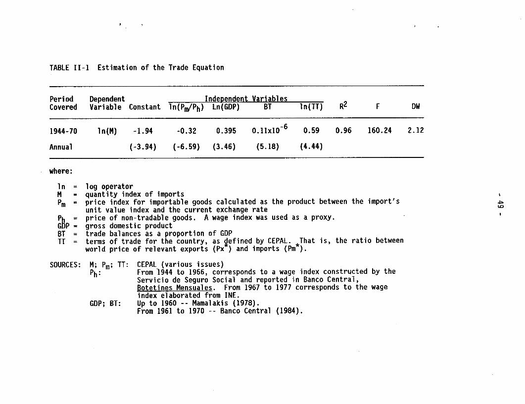
TABLE II-1 Estimation of the Trade Equation
Period Dependent Independent VariablesCovered Variable Constant ln(Pm/Ph) Ln(GDP) BT ln(TT) R2 F DW
1944-70 ln(M) -1.94 -0.32 0.395 0.llxlO 6 0.59 0.96 160.24 2.12
Annual (-3.94) (-6.59) (3.46) (5.18) (4.44)
where:
ln = log operatorM = quantity index of importsPm = price index for importable goods calculated as the product between the import's
unit value index and the current exchange ratePh = price of non-tradable goods. A wage index was used as a proxy.GAP = gross domestic productBT = trade balances as a proportion of GDPTT = terms of trade for the country, as defined by CEPAL. That is, the ratio between
world price of relevant exports (Px ) and imports (Pm*).
SOURCES: M; Pm; TT: CEPAL (various issues)Ph: From 1944 to 1966, corresponds to a wage index constructed by the
Servicio de Seguro Social and reported in Banco Central,Botetines Mensuales. From 1967 to 1977 corresponds to the wageindex elaborated from INE.
GDP; BT: Up to 1960 -- Mamalakis (1978).From 1961 to 1970 -- Banco Central (1984).

- 50 -
TABLE II-2 Import's Equivalent Tariff and the Liberalization Index
Equivalent LiberalizationTariff Index(t) (ordinal)
(percent)
1960 43.1 81961 43.1 101962 94.1 31963 94.1 31964 94.1 31965 94.1 31966 76.2 41967 76.2 31968 76.2 41969 38.6 51970 38.6 51971 56.7 31972 111.0 21973 182.2 21974 95.0 121975 95.0 121976 33.0 121977 20.0 151978 14.0 171979 10.0 201980 10.0 201981 10.0 -1982 10.0 -1983 17.5 -1984 25.0 -
SOURCE:
Equivalent Tariff: for 1960-73, were estimated according to themethodology reported in Appendix II; for1974 and 1975, it was taken from Sjaastad(1981); for 1976 and 1978, it corresponds tothe average values reported in Cauas and dela Cuadra (1981); from 1979 to 1984, theequivalent tariff was associated with theaverage value of the prevailing tariffs,since practically no variation existedbetween them on different products.
Liberalization Index: This is an index elaborated by Hachetteand de la Cuadra (1985). It isordinal, and its value increases as theliberalization process increases.

- 51 -
Appendix III
ESTIMATION PROCEDURE FOR PM/P*M
APPROACH
The objective of this appendix is to explain the procedure we
used to estimate the ratio of price of nonagricultural goods (actual
and undistorted) included in the calculations of indirect price
intervention.
To simulate free trade price levels for exportables and
importables (P* and P*), we had to make some adjustments on the
observed (distorted) prices Px and Pm.
Under free trade, the distorted Pm would change from
Pm*(1+t')Eo to P'*E*, where tm is the sector i's tariff prevailing in
a certain period (see Appendix IV for details in the calculation of
ti). Distorted prices in exportables would change from P,*Eo to
Pi*E*, while prices in the nontradable sectors would remain unchanged.
Therefore, the ratio between distorted and undistorted
nonagricultural prices (using Ph as numeraire) can be estimated as:

- 52 -
3 i 5 4i '
PNA n =1 a 1m i=1(A.24)
~NA 3 P E* .i 4 PNA X~~7 (Px, -) ax Xr ( _ a - Phai=1 Eo 1=1 1+tm Eo i=1
where:
PNA = Distorted prices of the nonagricultural goods.
pNA = Free trade prices of the nonagricultural goods
(assuming t = 0, and Eo = E*)
= Value added of imported nonagricultural sector i as a
proportion of value added generated by the aggregate of
the nonagricultural sector
c4 = Value added of exported nonagricultural sector i as a
proportion of value added generated by the aggregate of
the nonagricultural sector
ah = Value added of nontraded nonagricultural sector i as a
proportion of value added generated by the aggregate of
the nonagricultural sector
Pmi = Prices of imported nonagricultural sector i
Px = Prices of exported nonagricultural sector i
Pi = Prices of nontraded nonagricultural sector i
tm = Tariff on importable sector i (see Appendix IV)
E*/Eo = Real exchange rate misalignment due to both commercial
and macroeconomic policies

- 53 -
DATA SOURCES
The nonagricultural sectoral prices (Pi Pi, and Pg) are reported
in Appendix Table IV-7, the ails are reported in Appendix Table IV-8,
the import competing sector tariffs (ti) are reported in Appendix
Table IV-6, and the real exchange rate misalignment is reported in
Table 3-4. How Pm1 Px, Ph, ai's and ti's were obtained is discussedm'x tin
in Appendix IV. Appendix Table III-1 presents the resulting (PNA-
PNA)/PNA for the period 1960-82.

- 54 -
Table III-1 Nominal Rate of Protection ,NRP) in the Non-Agricultural Sector (PNA-PNA)/PNA
Year NRPNA
1960 -0.141961 -0.161962 -0.101963 -0.051964 -0.041965 0.001966 0.011967 0.001968 0.051969 0.041970 0.071971 0.001972 0.061973 0.191974 0.401975 0.321976 0.331977 0.211978 0.101979 0.091980 0.021981 -0.031982 -0.01
SOURCE: Appendix III

- 55 -
Appendix IV
ESTIMATION OF THE EFFECTIVE RATE OF PROTECTION
THE METHOD
For each activity the following expression is estimated for each
year:
i VA/VNA - VA/VNA
DNA * (A.25)VA /VNA
where:
VA = Value added of agricultural activity i, at prevailing
prices.
VA = Value added of agricultural activity i, at undistorted
(free trade) prices.
VNA = Value added of nonagricultural activities, at
prevailing prices.*VNA = Value added of nonagricultural activities, at
undistorted (free trade) prices.
DNA = Rate of relative protection enjoyed by the production
of agricultural good i with respect to nonagricultural
goods.
Expression 1 can also be written as:
DN ( VNA VI (A.26)VNA VA

- 56 -
where:
i = 1 + ERPA (A.27)
ERPA = rate of effective protection enjoyed by the(agricultural) activity i
and
VNA EaJVNAJ VNAJ= . . = EaJ . (A-28)
VNA EaJVNAJ j VNAJJ
where:
VNAJ = Value added of nonagricultural activity j, at
undistorted (free trade) prices.
VNA' = Value added of nonagricultural activity j, at
prevailing prices.
ai = Proportion of the nonagricultural value added of
activity j in the total value added of nonagricultural
sector.
By definition:
VNA3 1VNAJ 1 ~~~~~~~~~(A. 29)
VNAJ 1 + ERPNAJ
Therefore, aJ and ERPNAJ of each nonagricultural activity j needs
to be estimated, together with ERPA for each agricultural process i,
in order to calculate DNA, as required.

- 57 -
ESTIMATION OF EFFECTIVE RATE OF PROTECTION iN AGRICULTURE (ERPA)
The estimation of ERPA for each selected agricultural product
during the period analyzed is reported below. The tables that follow
present the basic data.
The effective protection rate enjoyed by activity i (ERPA) is
defined as:15
i i* i*ERPA = (VA - VA /VA ) (A.30)
where
iVA = Value added per unit of product i, at prevailing
prices.
VA = Value added per unit of product i, at undistorted
(free-trade) prices.
VA and VA can also be written as
VA = Pi ZPj aii (A.31)
VA Pi* -P aii (A.32)
where
Pi Actual prices of final good&i
Pi = Undistorted price of final good i
15 See Valdes (1973) and Hurtado et al. (1978) for a discussionof theoretical and empirical problems related to the estimation ofERPA in the Chilean agriculture.
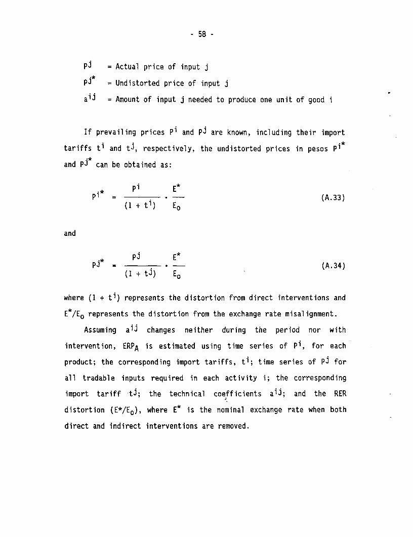
- 58 -
Pi = Actual price of input j
Pi = Undistorted price of input i
ai = Amount of input j needed to produce one unit of good i
If prevailing prices Pi and Pi are known, including their import
tariffs tl and tJ, respectively, the undistorted prices in pesos Pi
and Pi can be obtained as:
.* ~Pi E*pi* = . (A.33)
(I + ti) Eo
and
+ ~Pi E*PJ* = * (A.34)
(1 + tJ) E
where (1 + ti) represents the distortion from direct interventions and
E*/Eo represents the distortion from the exchange rate misalignment.
Assuming aii changes neither during the period nor with
intervention, ERPA is estimated using time series of Pi, for each
product; the corresponding import tariffs, ti; time series of Pi for
all tradable inputs required in each activity i; the corresponding
import tariff tJ; the technical coefficients ai3; and the RER
distortion (E*/Eo), where E* is the nominal exchange rate when both
direct and indirect interventions are removed.

- 59 -
DATA USED
Prices. Appendix Table IV-1 reports the information on Pi
(i.e., on tradable input prices, prevailing during 1960-84).
Output prices, Pi, for the five selected products are the same
used in the estimation of direct prices intervention, reported in
Appendix Table I-4. In the case of wheat, annual average prices are
used. For apples and grapes, the producer price at the FOB packing-
house level was used, according to considerations explained in
Appendix I.
Import Tariffs. Import tariffs for selected products, ti, were
obtained implicitly, as:
ti = (pi/pi*) - 1 (A.35)
where the Pi were adjusted following Appendix I, in order to make
them comparable with Pi. Both Pi* and Pi were used in the
calculations of direct price intervention.
In the case of wheat, two measures of direct price intervention
were reported in Table 3.1, depending on the interest rate used to
adjust border prices for seasonality. For the purpose of estimating
ERPA, the implicit tariff ti was estimated using the prevailing
interest rate, r(d).

- 60 -
In the case of beef production, the import tariff, assuming free
trade in live cattle, was used.
In the case of milk, the import tariff, assuming that the
implicit tariff prevailing in powdered milk is transmitted to producer
prices of fluid milk, was used, using the marketing model for milk
reported in Appendix I.
Finally, in the case of apples and grapes (exported products),
the "tariff" corresponds to the export and exchange rate subsidies
enjoyed by exporters during some years of the 1960-84 period. This
implicit tariff was measured at the FOB packing-house level, as
indicated in Appendix I.
Import tariffs on tradable inputs, ti, used in the estimation of
ERPA, are reported in Appendix Table IV-2. For some products and
years, these tariffs were obtained implicitly, comparing Pi with
adjusted Pi to take into consideration the importer's profit margin.
In some others, import tariffs were obtained from the relevant
legislation reporting tariffs and nontariff barriers to trade. The
general criterion for using one of the above criteria was the
following: In years when the tariff was "prohibitive" or when some
government institution was in charge of the domestic distribution or
trade, the implicit tariff was used for each product. Otherwise the
tariff reported in the relevant legislation was used. When more of
one tariff prevailed in some year, for a particular product, a
weighted average was estimated. Furthermore, other trade barriers as
specific import taxes and taxes expressed in "gold pesos," were

- 61 -
converted to its ad valorem equivalent.
Real Exchange Rate Misalignment. This was obtained in chapter
3, Table 3-3.
Input-Output Coefficients. Input-output coefficients for the
selected activities were taken from Hurtado et al. (1978). In some
cases (wheat and milk) two alternative technologies were used to
reflect more accurately the real production options open for that
activity. Appendix Table IV-3 reports the input-output matrix
employed.
ESTIMATION OF THE EFFECTIVE RATE OF PROTECTION OF NONAGRICULTURE
(ERPNA)
The definition of ERP iA, for each nonagricultural process i
follows from Expression (A.28) above. ERPNA was estimated using the
total transaction matrix for the Chilean economy in a base year, 1977
reported in Appendix Table IV-4.16
Essentially, the procedure uses the total transaction matrix in
the base year to identify trade flows, between thirteen consolidated
"industries," namely, agriculture; fishing; mining; food processing,
beverages and tobacco; textiles, clothing, and shoes; paper and
derivatives; chemical industries; nonmetal-lic and basic metals;
16 See Jeanneret (1971), Valdes (1973), De la Cuadra (1974) andHurtado et.al. (1978) for empirical efforts in estimating effectiverates for agricultural and nonagricultural processes.

- 62 -
machinery, equipment, and transport equipment; utilities;
construction; trade; and other services.17
Using, for each sector, all the information on intermediate sales
provided by the total transaction matrix, the effective protection
rate (ERPi) for each sector i (agricultural or not) can be defined as:
ERP1 = Vi* (A.36)vi*
where:
Vi = Pi Zaii Pi and (A.37)j
Vi* = pi* Zaii pi* (A.38)
The above expression can also be written as
ti + aii pj* Pti+ZaiJ - Z aliPi* . pi*
ERPNA = pi* (A.39)
1 - E aij
where:
Pi and Pi = Actual product price'of sectors i and j
Pi and Pi* = Undistorted prices of sectors i and j, after
17 The original matrix had twenty sectors. For the purposes ofthis study it was consolidated into thirteen sectors, by aggregatingthe public administration and service sectors. Agriculture has to beincluded because of its transactions with other sectors.

- 63 -
removing both commercial policy and exchange rate
interventions
aii = Input output coefficient indicating the amount of
input (produced by sector) j required to produce
one unit of output in sector i
ti = Import tariff applicable to the product generated
by sector i
As is known, each row j of this matrix indicates the value of the
sales that sector j makes to each other sector i of the economy.
Therefore,
Sji = Pi aij Qi (A.40)
where:
Sii = value of sales that sector j makes to sector i
Qi = quantity produced by sector i
The total transaction matrix also provides information on PiQi,
the gross value of production in each sector i of the economy.
For each pair of sectors (i,j) the following ratio was available
pi aii Qi Pi aii (A.41)
PiQi pi
As reported in Appendix II, the tariff structure for the Chilean
economy in 1977 was quite simple, because it was characterized by a
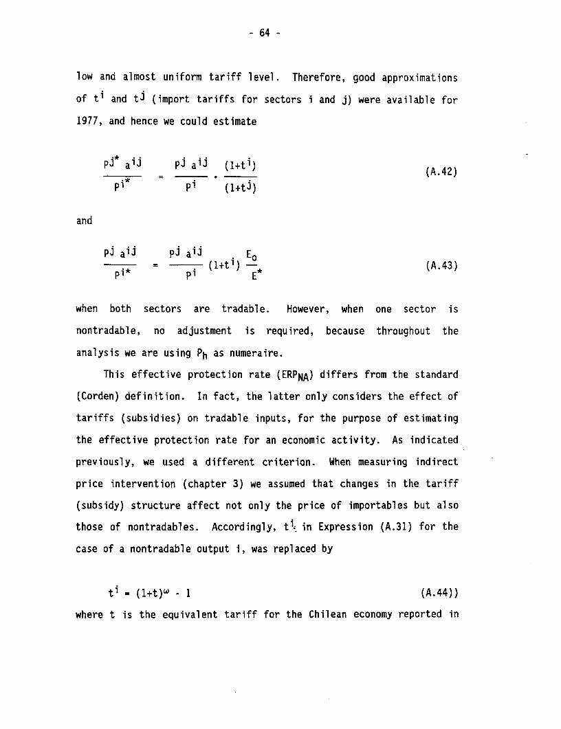
- 64 -
low and almost uniform tariff level. Therefore, good approximations
of ti and ti (import tariffs for sectors i and j) were available for
1977, and hence we could estimate
PJ aiJ Pi ai3 (l+ti) (A.42)
pi* pi (1+tj)
and
Pi ai3 Pi a1J Eop1* = P (1+tl) -E (A.43)
when both sectors are tradable. However, when one sector is
nontradable, no adjustment is required, because throughout the
analysis we are using Ph as numeraire.
This effective protection rate (ERPNA) differs from the standard
(Corden) definition. In fact, the latter only considers the effect of
tariffs (subsidies) on tradable inputs, for the purpose of estimating
the effective protection rate for an economic activity. As indicated
previously, we used a different criterion. When measuring indirect
price intervention (chapter 3) we assumed that changes in the tariff
(subsidy) structure affect not only the price of importables but also
those of nontradables. Accordingly, ti; in Expression (A.31) for the
case of a nontradable output i, was replaced by
ti = (1+t)w - 1 (A.44))
where t is the equivalent tariff for the Chilean economy reported in

- 65 -
Appendix Table II-2, and w is the Sjaastad transmission coefficient
relating changes in nontradable prices resulting from changes in the
price of importables.
Similarly, for the case of a nontradable input j used in the
production of a tradable good i, the ratio Pi*/pi in Equation (A.31)
was replaced by:
Pi* Pi (l+ti) Eo-*a J=-aJ
pi pi (1+t)w EA
Estimation of DiA for the Rest of the Period 1960-84. Assuming
fixed aii for the period under study, ERP, and therefore Expression 1
for each selected product, can be estimated for the rest of the years
of the period 1960-84.
Knowing Equation (A.32), for 1977, the assumption of fixed aij
allows the estimation for the rest of the period, because this ratio
will change with the evolution of Pi/Pi, the relative prices of sector
j and i, respectively. Therefore, knowing the evolution of the
appropriate price indexes, Equation (A.32) can be estimated for each
year.
To estimate ERP, appropriate estimations of ti and ti are also
needed, for the 1960-84 period. Clearly this is the more complicated
step, because the tariff structure for the Chilean economy during
1960-75 is characterized by high tariff dispersion and the generalized
use of quantitative and nontariff restrictions on trade. Therefore,
some simplifying assumptions were made to solve this information
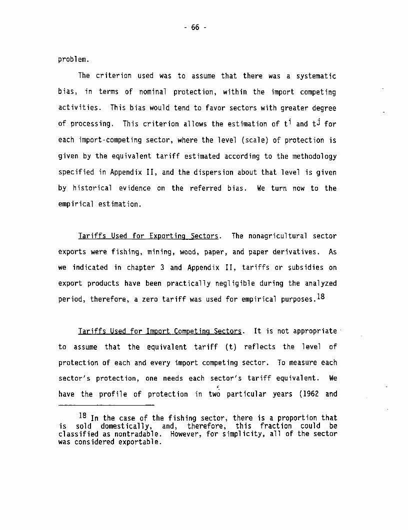
- 66 -
probl em.
The criterion used was to assume that there was a systematic
bias, in terms of nominal protection, within the import competing
activities. This bias would tend to favor sectors with greater degree
of processing. This criterion allows the estimation of ti and ti for
each import-competing sector, where the level (scale) of protection is
given by the equivalent tariff estimated according to the methodology
specified in Appendix II, and the dispersion about that level is given
by historical evidence on the referred bias. We turn now to the
empirical estimation.
Tariffs Used for Exporting Sectors. The nonagricultural sector
exports were fishing, mining, wood, paper, and paper derivatives. As
we indicated in chapter 3 and Appendix II, tariffs or subsidies on
export products have been practically negligible during the analyzed
period, therefore, a zero tariff was used for empirical purposes.18
Tariffs Used for Import Competing Sectors. It is not appropriate
to assume that the equivalent tariff (t) reflects the level of
protection of each and every import competing sector. To measure each
sector's protection, one needs each sector's tariff equivalent. We
have the profile of protection in two particular years (1962 and
18 In the case of the fishing sector, there is a proportion thatis sold domestically, and, therefore, this fraction could beclassified as nontradable. However, for simplicity, all of the sectorwas considered exportable.

- 67 -
1967). The evolution of protection over time for each sector is
assumed to change in the same proportion as changes in the equivalent
tariff.
However, there is a possibility of systematic bias. To check for
such a bias, we analyzed the available information on tariff structure
for 1962 and 1967.19 As reported in Appendix Table IV-5, there is a
consistent ranking of each sector, according to its nominal
protection. Textiles and machinery and equipment showed higher
protection rates, whereas metals and chemical industries were lower.
This is consistent with policies implemented during the analyzed
period, which had the objective of providing more nominal protection
to sectors with higher degrees of processing (e.g., tariff
escalation).
To generate a tariff dispersion around the equivalent tariff
available for each year (in nonagricultural import competing sectors)
the following procedure was used. First, for 1960-61, it was assumed
that tariff for each import competing sectors kept the same proportion
with the tariff equivalent that prevailed in 1962, reported in
Appendix Table IV-5. Second, for 1968-73, we assumed that tariffs for
each import competing sector kept the same proportion with the tariff
equivalent that prevailed in 1967. Third, for 1963-66, a linear
interpolation between proportions prevailing in 1962 and 1967 was used
19 For those two years, existing studies had estimated advaloremtaxes for different sectors, using indirect mechanisms (implicittariffs). See Jeanneret (1971) and De la Cuadra (1974) for basic dataused in this study.

- 68 -
(see Appendix Table IV-5). Finally, from 1974 on, the tariff
dispersion was obtained based on a revision of the relevant
legislation that followed the process of liberalization, as reported
in Causas and De la Cuadra (1981).
A different criterion was used in the case of the agricultural
sector. Clearly, for present purposes, what should be measured
ideally is not the average nominal tariff relevant for total
agricultural output but specifically the tariffs of products that
agriculture sells to other sectors, in the context of the matrix of
trade flows reported in Appendix Table IV-4. We chose the latter,
because the effective protection rates of the selected agricultural
products has already been estimated (see Tables 3-2 and 3-6).
Inspection of Appendix Table IV-4, reveals that food processing
is the principal buyer of agricultural output. Therefore, for the
whole matrix, in estimating agriculture as an intermediate input, we
used the composition of agriculture sales to this sector to estimate a
weighted average for the agricultural tariff, which we then used to
estimate the effective protection of the nonagricultural sectors. The
weights were estimated based on same evidence reported in Departamento
de Economia Agraria (1983) for 1977, and were assumed constant
throughout the period. This assumption might be especially strong in
those years where relative prices differ significantly from the 1977
situation. We should note that this approach describes the estimation
of protection for the nonagricultural sector. In the estimation of
ERPA, the approach corresponds to that described earlier in this

- 69 -
appendix.
A final comment must be made with regard to the procedure used to
assign a particular import tariff to each one of the thirteen economic
sectors. The criterion was imposed by the availability of relative
price indexes needed to estimate Equation 8, in each year. For
example, in case of food processing, beverages and tobacco the price
index available was only appropriate for food products (wholesale
price index of food, reported by INE), and therefore the tariff used
was the one relevant for food only and not the one resulting from the
average between food, beverages, and tobacco. Similarly, in the case
of textiles, clothing, and shoes, because price indexes were available
only for textiles (wholesale price index for textiles, reported by
INE), the tariff of this particular subsector was used for the
complete sector.
The nominal import tariffs for import competing industries used
in this study are reported in Appendix Table IV-6.
Price Indexes Used. Price indexes used to reconstruct Equation 5
for each year are reported in Appendix Table IV-7. The following
criterion was used:
First for the exporting sectors, relevant price indexes for
exports were used. Because export tariffs or subsidies on exports
were not significant during the analyzed period, it seems reasonable
to assume that domestic prices of exportables move together with price
indexes of exports, in a particular product, using the official

- 70 -
exchange rate to convert export prices into domestic ones.
Second, for the agricultural sector, the relevant (agricultural)
component of the wholesale price index was used.
Third, for import-competing sectors, the relevant subindexes of
the industrial wholesale price indexes were used. Because these
subindexes were not available for the period 1960-67, they were
constructed based on available information on particular products,
using the same weights of the relevant index for 1968-82.
Fourth, for nontradable sectors, some implicit deflators for
nontradables used in national account were used. In the case of the
construction sector, a particular price index generated by Camara
Chilena de la Construccion was used.
The Value of ai. Finally, a& included in Equation 3 was needed
to estimate VNA/VNA and DNA specified in Equation (A.26).
In general, the value of ai for a particular sector was taken
from the National Account Statistics reporting the incidence of each
sector in the total nonagricultural value added.
For the particular case of manufacturing sector, the above
information is too aggregated for present purposes. Therefore, for
1960-70 the weights were taken from Corbo and Meller (1981) and from
Meller et al. (1984) for the period 1974-81. For 1971-73 the same
weights of 1970 were used, whereas for 1982, ai of 1981 was used.
Finally, in the few exceptional years where ERPs calculated as in
Equation (A.31) could not be obtained (cases of negative value added

- 71 -
in the distorted and undistorted situations), the ERP immediately
before or after was used in the weighted average.
The sectorial proportions within GDP and within the manufacturing
sector are reported in Appendix Table IV-8, expressed as a percentage
of nominal value added for each year.
Real Exchange Rate Adjustments. These were discussed in chapter
3 and reported in Table 3-3.
METHODOLOGICAL LIMITATIONS
The methodology employed to estimate ERPs and therefore DNA has
at least two limitations that deserve consideration.
Ranking of Tariffs. The procedure used to generate dispersion
around the level of the equivalent tariff can be defendable in a
qualitative basis, because it captures the fact that historically not
all import competing sectors have enjoyed the same level of
protection. However, from a quantitative point of view, the
limitations of the methodology employed are clear. It is far from
obvious that the particular tariff structure generated around the
equivalent tariff is consistent with the latter. In fact, the
definition of the equivalent tariff establishes that it is the tariff
that if applied uniformly to all importable sectors would reproduce
the same volume of imports that effectively prevailed in each year

- 72 -
(although not its composition). Therefore, for a particular ordinal
ranking of tariffs, only some of the infinite combinations of tariffs
will satisfy this condition, and no test has been performed to check
if the particular one used in this study is feasible, from that point
of view.20
The above criticism is more valid for the period 1960-73 than for
1974-82. In the latter period, our ranking followed the actual
evolution of sectorial tariffs. Yet, no alternative procedure was
found for this critical subperiod.
The Treatment of Nontradables. It was assumed that changes in t
would affect the relative price between tradable and nontradable goods
by (1+t)w. However, for some sectors, this assumption seems
unrealistic. In particular, prices in the public utility sector are
fixed by the authorities and probably do not react to commercial
policies, as is implicitly assumed with the use of w. In this sense,
the methodology employed may lead to incorrect conclusions, because it
assumes that under free trade, the price of nontradables (e.g.,
utilities) would have fallen in relation to the price of exportables.
The limited empirical evidence available in Chile does not support
this conclusion. Typically, policies in the direction of free trade
have been implemented together with self-financing measures in public
enterprises. The final result is that relative prices of these types
20 Direct and cross-price elasticities of supply and demand ineach sector of the economy would be required to perform this test,which is not empirically feasible.

- 73 -
of nontradables have increased in relation to those of exportables.
Perhaps it would have been more appropriate to consider those prices
as exogenous and to include them in the value added for purposes of
estimating effective protection in the nonagricultural sectors.
For the rest of nontradable sector (services, trade, and
construction), the methodology employed seems reasonable. Therefore,
global results should not be significantly distorted by the inaccurate
treatment of public utilities.

Table IV-1 Domestic Nominal Prices of Tradable Inputs Used in the Estimation of Effective Rates of Protection in Agricultural Sector
Milking Cattle
Year Nitrogen Phosphorus Insecticide Herbicide Fungicide Tractor Machinery Oil Breeder
(S/ton of N) (S/ton of P205) (S/application on wheat) (S/unit) (S/unit) ($/1000 Its) ($/head)
1960 0.438 0.108 0.00182 0.00168 0.00301 6.809 7.654 0.04367 3.904
1961 0.301 0.115 0.00173 0.00159 0,00286 5.555 6.239 0.04367 3.498
1962 0.337 0.141 0.00208 0.00192 0.00345 5.790 6.509 0.04525 3.432
1963 0.589 0.250 0.00322 0.00296 0.00533 9.009 10.128 0.06452 5.251
1964 0.832 0.372 0.00505 0.00461 0.00828 15.26 17.158 0.08407 11.53
1965 1.06 0.370 0.00626 0.00576 0.0104 30.06 33.68 0.10115 17.84
1966 1.43 0.815 0.00868 0.00799 0.0144 24.22 27.27 0.1199 23.00
1967 1.6 0.931 0.0125 0.0115 0.0206 30.68 55.13 0.1479 26.32
1968 2.2 1.02 0.0278 0.0256 0.0461 45.05 84.72 0.1964 38.08
1969 2.9 1.62 0.0375 0.0345 0.0620 98.11 185.90 0.2474 42.74
1970 3.7 2.14 0.0444 0.0428 0.0770 131.03 206.23 0.3494 59.04
1971 3.9 2.32 0.0704 0.053 0.0996 86.63 97.44 0.3791 86.11
1972 10.3 6.92 0.0933 0.12 0.050 224.7 252.50 0.4709 166.3
1973 157.9 78.65 0.847 1.03 0.355 2026.4 2278 4.886 990.1
1974 1158 945.8 5.585 5.97 1.5 10588 10512 67.97 9877.2
1975 4934 5164 36.28 29.3 10.9 64661 61862 494.8 41504
1976 7641 5889 79.78 105 45.9 141731- 149127 1516 79626
1977 11120 6449 154.1 147 265 222119 228883 2372 177705
1978 18690 11100 206.1 231 260 325997 366464 3571 245391
1979 26520 19130 289.5 314 451 507948 571001 8152 480250
1980 35103 27274 369 414 488 676856 760877 11766 644801
1981 39389 38207 463 532 623 611202 687072 12260 705051
1982 40219 44929 546 616 754 1260224 1298031 14260 803663
1983 58930 69853 921 827 1098 2092866 2155652 21631 1216631
1984 88309 85972 1146 938 1424 2771273 2854411 27469 906809
1/ All prices exclude the value added tax.
2/ Prices of Nitrogen and phosphorus correspond to a weighted average from different sources of fertilizers used in the country (urea and sodium
nitrate, basically.)3/ Information of pesticides (herbicides, fungicides and insecticides) is rut available in Chile, on a consistent basis, before 1976. Therefore an
indirect approach was utilized to reconstruct the time series. In general, a basic price of the application in 1977 was available from Hurtado
et. al. (1973). This price, adjusted by tariff and marketing margins was moved for the rest of the years according to the variation on the unit
values of imported pesticides, obtained from Aduana de Chile. This inplies the assunption that each conponent of the pesticide groups moves
together with the average, which Is reasonable based on enpirical evidence. The marketing margin utilized was 40 percent, constant during all
periods. The import tariffs used are reported in Table IV-2
4/ Oil price corresponds to the wholesale level, reported by INE.
5/ The time series for tractor prices was obtained from FAO. Trade Yearbook (many Issues), that reports the CIF average price for each year. This
price was incremented in the iport tariff (see Table A6-2) and a marketing margin of 38 percent obtained from Machinery importers. In the
estimation of effective protection rates, the price of the tractor-day was required. This was calculated using information given in Bemedetti y
Gallegus (1983) for length of equipment's life and residual values. A rate of interest of L18CR plus 6 percent annually was used to estimate the
opportunity cost of capital.6/ The treatnent for milking machinery ves similar to that of the tractors, adjusting the CIF prices by inport tariff of this type of equipment (see
Table IV-2) and marketing margins. A value of 33 percent was used.
7/ Price of cattle breeders was established in relationship with the price of meat, following itirtado et al. (1978) indications for 1977. This
relationship allowed the completion of the series for the rest of the period. These c.i.f. prices were adjusted by marketing margins (25
percent) and the import tariffs (see Table IV-2) prevailed in each year.
8/ Prices of wheat seed and cattle feed sepplementation are rut included in the above Table even though they are basically traded inputs. Both
prices were derived from wheat prices using the price relationship prevailing in 1977 reported in iurtado et al. (1978). The time series was
reconstructed for the rest of the period using a marketing margin of 10 percent for cattle feed supplementation and 15 percent for wheat seed.
Also isport tariffs of wheat were used to adjust these items.
SOURCE: Information Center. Department of Agricultural Economics Catholic University of Chile.

- 75 -
TAIIE I-2 nxrt Tariff of Tradble Irpits Uth to Estinte the Effawtive Prtstim Rates of Aricultbul Swtor
IHlkirg CattleYear Nitroge Pixai*uus Pesticiis Oil Trn±rs luiry Brs
(-n )
1960 -17 -42 0.6 74 0 0 51961 -5 -39 0.8 67 0 0 51962 10 -31 0.6 40 0 0 111963 14 -31 0.6 44 10 10 4195A 15 -35 0.6 53 27 27 21965 11 -36 0.6 34 10 10 121966 32 1 0.6 27 53 53 121967 27 27 10.9 27 47 35 15196 55 5 20 25 56 61 201969 72 5 20 19 56 63 01970 8 5 20 30 55 17 201971 10 so 16.3 9 -22 -22 561972 2B 55 16.3 -18 40 40 601973 327 -38 24.8 12 6 6 6D1974 0 0 42 -31 39 33 201975 5 5 44 -9 41 38 201976 5 5 37 -4 25 25 171977 9 9 20 -13 20 17 101978 11 10 16 -13 10 10 101979 10 10 15 32 10 10 101980 10 10 15 14 10 10 10198 10 10 15 10 10 10 101972 10 10 10 2 10 10 101953 17.5 17.5 17.5 12 17.5 17.5 17.51984 25 25 25 17 25 25 25
1 All tariffs are aq3ssad as a peait wlue an the c.i.f. pice.(For mm ys amior pr1asts, iort tariffs em estita implicitly. i.e.. ixWring c. i.f. pioe aLited by mratir t inagins wth
detic pries. In the rest of the a, imrt tariffs mm d*tairad by reising the rleit lgislatin. lh gal criOterio ttfollowing: (i) if tariff m prcibitive or if a g mesnagt ag ws in duro the _3 keting of the piut. pirort tariffs weesttad iplicitly as indicatei abiw, (ii) im the tariff s ti. fri. the elant lgislatic anaml aa tariffs mm odbainedby weighting the tariffs by the .ubr of uId in the ewr tht tle tariff pneailsd. llhe rupiit of previoas kpiuts (psitospevi&.) ard tam eqpresss in 'gold pesos m calculated aid o nweted in a&-mlar taiff euiwlents.lh Ih folloeing criteria em umed fcr ec of th irpits:Ni tn: 19D-73. bpl icit tariff s estited using a lceting argin of 15 pa cat. Fri thEe an tariffs m d*tained frm th
relewat legislation.Is~~: For all yaers tariffs we dtained fru th3 releAt legislatiwn. ept fcr 1972-73. We a 10.C0O pc.wt previous dqoit
fcr 240 days v irp1 l. For this er, the tariff ws est i ispl icitly using a 15 pecot rketing margin.Pesticides: For 1960-70 tariffs were otaine frtc relevit legislatici. For 1971-73 the tariff mm esti ispl icitly Lsinig a 40 pmzct
i*eting rgin. Fcm 1974 to 1984, tariffs wre again bairnd from th lgislatian.Oil: lOpl icit tariffs wee tained for the udwle period, simu a gnt eteipriss (EW) had the Ily of distributicn. A
6.5 peir.t mketing mwrgin usmed.Tractcrs aid Nilki
chik : For 1960-70 tariffs ere btaism ft relevant lgislation. For 1971-73 th tariff s est it ictly. using a 2B peastmedreting wrgin, sine a 10.000 penet previaos dieoit the leal tariff pr*hibftive. Frau 1974 cn tariffs me aginobtainBd frcm th legislation.
Catleers: For th idmle period tariffs we itained fr. t relevant lgislation.
mt Sed aid CattleFecd Stalenntatig: For ftNme be bpits (not aring in the table) udt tariffs we ulx as a pnxy.
91 : Est'it fcr this stLy using varias saos.

- 76 -
TABLE IV-3 Input-Output Coefficients Used in the Estimation of Effective Protection Rates of the Agricultural Sector
OutputInput Wheat Wheat Cattle Milk Milk Apples Grapes
1 2 - 1 2 - -
(tons) (tons) (tons) (1000 lt.) (1000 lt.) (tons) (tons)
Tractor Use (machine days) 0.635 0.52 0.98619 1.0526 0.8566 0.5104 0.2751
Oil (1000 lt.) 0.0294 0.024 0.039448 0.0421 0.03426 0.0204 0.0110
Nitrogen (tons N) 0.0512 0.03072 0.02032 0.0081 0.3421 0.03167 0.07739
Phosphorus (tons P205) 0.047 0.06016 0.06092 0.06291 0.0664 - -
Seed (kgs.) 100 80 - - -
Herbicide (application) 0.5 0.4 - -
Insecticide (application) 0.5 0.4 - - - 0.6997 0.2786
Fungicides (application) - - - - - 0.48882 0.1774
Milking Machinery (units) - - - 0.00127 0.00113 - -
Cattle (tons, live) - - 0.5953 0.20027 0.1827 - -
Breeder (units) - - - 0.00317 0.00231 - -
Cattle Feed Supplementation - - - 208.43 186.35 - -(kgs.)
I/ To reflect alternative technologies used in the country two options were included in wheat and milk production. A brief
description of the included processes is:
Wheat 1: white wheat, labor-intensive technology, region VIIIWheat 2: white wheat, machinery-intensive technology, region XCattle: corresponds to a fastening process; initial and final weight are 250 and 420 kg., respectively; based essentially
on grazing and winter supplementation with clover hayMilk 1: mixed system of production, generating milk and meat, used typically in region XMilk 2: mixed system of production, generating milk and meat, used typically in the central valley of region VIIIApples: production oriented to export; standard technology
Grapes: production oriented to export; standard technology
V The tractor's coefficients used includes harvesting machines.
ai The coefficient for insecticide and fungicide, in the case of apples and grapes, is expressed in kgs., and not in nuTber ofapplications.
gJ The coefficients for cattle in the milk 1 and milk 2 process have negative signs, indicating that meat production
increases the value added in the process of milk production.
SOURCE: Hurtado, H. et al. (1978) Analisis de la Estructura Arancelaria en la Acricultura Chilena. Serie de InvestigacionesNo. 28, Departamento de Economia Agraria, Universidad Cat6lica de Chile. Minor modifications were made in the case of
apples and grapes, where an error was discovered in the original study.

Table IV-4 Total Transaction Matrix of the Chilean Economy (1977)
Sector (1) (2) (3) (4) (5) (6) (7) (8) (9) (10) (11) (12) (13)
(S millions)
(1) Agriculture 5411 14 77 21552 1194 1523 165 12 35 5 76 6 1443
(2) Fishing '.0 212 0 1539 0 0 11 0 0 0 0 0 150
(3) Mining 392 0 3274 319 31 32 11447 3245 138 463 432 3 140
(4) Food Processing,
Beverages, and
Tobacco 1631 103 44 13465 524 13 263 28 31 8 18 581 5693
(5) Textiles,
Clothing,
and Shoes 141 78 140 237 6957 199 482 26 205 39 112 307 775
(6) Paper, Paper Pro-
ducts, Wood, and
Printed Matter 202 11 164 1419 347 4627 567 228 405 48 1890 1718 2822 1'14
(7) Chemical
Industries 2771 352 4976 2494 1879 1722 7157 751 1330 1488 1636 1503 11813
(8) Non-Metallic
and Basic Metals 61 17 1560 308 34 114 386 1753 3379 75 4595 38 514
(9) Machinery,
Equipment, and
Transport Equip. 1134 255 3841 1513 462 605 806 512 4103 322 1807 1383 10257
(10) Utilities 196 1 1907 453 300 367 223 354 286 1977 111 569 1664
(11) Construction 0 0 386 2 0 167 23 115 0 6 23 356 4063
(12) Trade 8726 921 213 9584 6065 1466 9718 1016 3216 2 0 0 39
(13) Other Services 1143 97 2810 3114 981 2005 1980 1104 1433 307 1331 8805 23553
Value Added 26837 1453 23161 22282 7468 8937 10273 4194 9419 6477 11706 44844 96728
Gross Production
Value 48645 3514 42553 78308 26242 21777 43501 13338 23980 11217 23737 60113 159656
SOURCE: ODEPLAN (1977) Matriz de Insumo Producto de la Economia Chilena.

- 78 -
TABLE IV-5 Nominal Protection Rates for Selected Import CompetingSectors
Sector 1962 1967
(percent)
Food Processing 82 32
Textiles 182 99
Chemical Industries 67 32.5
Non-Metallic andBasic Metals 66 25
Machinery andEquipment 1/ 91 123
Economy Z/ 94.1 76.2
1/ It corresponds to a simple average of the protection ratesof non-electrical machinery, electrical machinery, andtransport equipment.
2/ It corresponds to the Uniform Equivalent Tariff calculatedin previous chapters (see Appendix II for more details).
SOURCE: Jeanneret, T. (1971) and de la Cuadra, S. (1974).Figures for 1962 come from a Jeanneret study carriedout at the end of 1961. For this reason these tariffsare a better reflection of the protection structure of1962.

- 79 -
Table IV-6 Nominal Import Tariff for Import Competing Industries
Non -Metallic
Food and MachineryAgri- Pro- Chemical Basic and
Year culture cessing Textiles Industries Metals Equipment
(percent)
1960 71 38 83 31 30 421961 72 38 83 31 30 421962 77 82 182 67 66 911963 77 73 169 61 59 1041964 68 65 158 57 52 1161965 25 57 146 51 45 1271966 16 40 109 37 31 1131967 1 33 99 33 25 1231968 -2 33 99 33 25 1231969 -3 17 50 17 13 621970 19 17 50 17 13 621971 4 24 74 24 19 911972 -11 48 144 48 37 1791973 -23 78 237 78 60 2931974 -8 83 141 18 60 1501975 10 56 84 18 42 991976 8 30 47 16 32 601977 18 18 31 3 20 361978 16 12 18 0 13 191979 24 10 11 21 10 111980 13 10 10 12 10 101981 3 10 10 10 10 101982 4 10 10 6 10 101983 7 18 18 15 18 181984 35 25 25 21 25
SOURCE: See Appendix IV

TABLE IV-7 Price Irdices Lbod to Eatinuts Effeti.e Rates of Protetim for the Nb-AGicultumrl Sector
Yer Agriclture Fluillrg Miniri Food Tmcti lee P4er ard Unical Ibn-etllc ard Mchimery Eqilpnart d Utilities Corstructin Canrrce OtherPr.esirg DaHvitlve Irdrsfrlu Bsic Vtals Tra40rtatlon Eqjlprnnt Serv ice
ll) (2) (3) (4) (5) (5) (7) (7) (8) (9) (10) (11) (12)
ISD 18.23 13,5 10.33 14.92 18.88 14.21 22.43 18.86 15.35 14.84 12.58 14.93 11.89
198 18.31 14.95 9.87 15.35 18.89 15.54 22.41 15.82 15.39 18.25 13.32 15.31 13.35
m2 18.44 11.05 10.95 17.72 17.24 17.28 23.49 18.80 15.22 20.92 15.07 17.08 15.41
193 28.54 18.3 18.05 25.3 22.13 25,18 32.02 23.29 23.58 23,58 21.6 25.13 22.04
i194 40.22 23.95 25.17 37.35 33.70 32.92 43.12 23.99 32.71 32.52 32.85 38.27 32.71
1n 55.24 36.85 37.53 50.48 36.97 41.65 82.54 35.28 44.12 58.1 45.28 S0.00 45.62
m9 9.44 57.31 5. 10 85.58 e2.43 89,02 e2.99 51.13 58.41 74.83 59.84 60.s5 59.72
1887 8D.43 189.8 72.57 78.2 78.97 75.16 78.33 70.99 74.95 85.81 75.00 72.97 75.23
195 100 100 100 1O 100 100 100 ID 10 ID0 too 100 100
198 141.0 111.8 153.3 1.34 13.2 139.0 131.1 140.1 145.8 111.3 15.2 136.7 134.5
1970 191.7 148. 210.7 179.3 183.2 195.1 160.5 212.9 MS6.7 149.1 190.1 198.1 192.5
1971 240.6 177.8 15.1 a09.2 195.4 222.4 160.1 238.2 221.1 L58.9 255.7 213.4 258
19n 52.1 237.8 282.3 385.5 274.9 33.6 248.1 299.9 278.4 182.8 522.1 405.2 455.1
1973 2753 2128 2121 1951.2 m3s 18S 021 1727 78 192.1 2879 229 1955
1974 20372 23958 2240 21850 17300 38774 3010 233a4 13812 8170 18919 1550 14643
1975 M3M3 1s3891 83715 54740 5500 155 19 880 3750 5717 81091 5414 72314
1978 470207 345474 258873 177040 198970 47455 23GIIZ 232G00 121480 188sm4 27518 27397 245305
1977 842982 5883 3B372 3150 35290 771819 5848 35873D 225540 39880 5714 505380 544388 O
1978 1135370 77no8 516047 45280 5i830 11800 83344 455850 3S270 573620 885855 758s19 600054 0
1979 172m 1181834 105510 S5470 751810 198341 107400 8s47M 425910 792115 12538 1091705 1314535
seD 233044D 1471980 1232482 945480 1019O 2744717 2059400 910586 581050 100502 1777893 1322949 181251
18 23s3s2 1374456 1OD4178 979250 11s1 278 231500 92 860 839830 1070956 2177919 1528935 221381
1982 2411177 1323814 1151138 1142100 1227980 257505 288380 1025600 705030 L507405 2299718 1742158 2512345
1983 3647860 1957M 1859 1482180 1608200 32U41D 4073900 15940 995070 1917773 222820 2118888 2881105
1984 4412413 2457045 197894 1841854 19505 40 511358 2053581 1240283 10988 n.e. n.a. n.a.
Sctor 1: INE, Whialle price lbx of Agricultml Prr1aXts.Ssctors 2, 3, and 5: Sm (1965); c'ebqaih to prime 1rms of poWted gbds.Sector 4: INE, "lale pric uitd. Fa 198 to 1952 cwoqrn2x to th w lealb pric irdm o fbd proutst. Fnn 1950 to 1958 this irdc me rat available, so a prW au
catnxtW usig ths folloV1rg criteria:(I) to lmacnb thm larst maiar of gd avwilable for the purlod 196D-I , lmlubd in the 1958-1982 ird.(11) to weugit thse prim usirg the -o r latiw wuIgte thit ts hod in the 198-1502 iwbx.The pecnta wwr d vat 54.8 pwnt of thI 1988-192 wer4p.
Sswtor : INE, wholesele pric lnrdx. Fran 19E8 to 1992 c rnx a to thn wtleal prico Index of tetile prodJcts. Fran 1 to 1988 it as also rouamry to cnstruct a praW inrdx.
This v1S cbx follArl then critwia und In rector 4. ThN paromtsp owrd we 28.6 pmrcent.wector 7: IE, whDtcble price Irdc. Fmn 1958 to 192 cr.oDnrs to the wholesle prime irdK of chol bls awd drived pricts 1ran petrolam Fran 198 to 1988 a pray Index wss
ocmatnucta follwirg thI natnad already bcribd. Trh wrep me 55.8 pucs,t.Sectar 8: INE, wholmle price lndx. Fran 19 to 192 ooarenpai to the vihmle price 1ndex of netallic prajtse. Frmm 19E0 to 1958 thn pron lrdr cmstructed had a coAwre of 33.9
Sector 9: INE, Wolle price indx. Fra 19f to 1982 corrn q=db to the Whileals price lnx of electrical plprmt rd tools. Frgm 1990 to 1988 th proxy Irbx wotntctd wrwed the
52.7 prmmnt.Swtar 10: INE, Wolmals price lidsx. oDnespDrds to the prlo of the killtt/hIur.Sctor 11: Cara Chillma c la arstrimcicn. Carreqads to a buildirg coet unit.

Table IV-8 SectDral Participation in GCP arid Manufacturing Irdustries
Participation in GIP Participation in Marufacturing Indistry
Non-Metal l ic
Maeu- Paper aid Machinery
facturing Co- Other Food Pro- ard Deri- Chsnical Basic aid
Year Fishing Mining Indistry struction Utilities Comarce Services cessing Textiles vatives Indistries Metals Equipnent
1960 0.4 8.0 21.8 4.6 1.5 22.8 28.7 18.2 26.6 9.1 8.8- 13.6 18.8
1961 0.3 7.2 22.2 4.9 1.6 22.3 28.8 18.2 26.6 9.1 8.8 13.6 18.8
1962 0.3 6.8 23.6 5.5 1.7 21.4 28.6 18.2 26.6 9.1 8.8 13.6 18.8
1963 0.2 8.2 23.7 6.0 1.7 21.6 28.2 16.7 24.6 9.3 9.4 14.3 21.3
1964 0.3 8.2 24.3 5.9 1.9 20.7 28.3 16.7 24.6 9.3 9.4 14.3 21.3
1965 0.3 7.7 23.8 6.0 2.3 19.2 29.6 16.7 24.6 9.3 9.4 14.3 21.3
1966 0.4 8.7 22.8 5.5 2.2 19.2 29.2 18.1 22.4 10.5 10.9 10.7 24.3
1967 0.3 8.9 23.6 5.1 2.1 18.5 29.8 18.1 22.4 10.5 10.9 10.7 24.3
1968 0.3 8.7 25.4 5.1 1.9 18.7 29.5 18.1 22.4 10.5 10.9 10.7 24.3
1969 0.3 10.8 25.1 4.9 2.0 18.7 28.9 17.3 20.8 10.8 11.7 10.8 25.7
1970 0.3 8.8 25.5 5.1 2.0 18.6 29.9 17.3 20.8 10.8 11.7 10.8 25.7
1971 0.5 5.8 24.4 6.1 2.2 18.0 32.8 17.3 20.8 10.8 11.7 10.8 25.7
1972 0.4 6.8 23.4 " 6.2 1.5 18.2 32.3 17.3 20.8 10.8 11.7 10.8 25.7
1973 0.3 9.2 27.1 4.3 0.5 20.8 28.8 17.3 20.8 10.8 11.7 10.8 25.7
1974 0.4 12.0 29.5 6.1 1.1 14.1 27.9 18.9 9.2 5.9 13.5 37.5 14.7
1975 0.3 10.4 20.3 5.4 2.1 17.3 34.2 22.0 8.0 7.0 22.1 26.0 14.5
1976 0.4 10.2 23.3 4.3 2.3 15.1 32.5 23.4 9.1 9.4 20.5 19.7 17.5
1977 0.5 8.1 21.7 4.1 2.3 15.6 33.5 27.0 9.8 8.7 17.7 19.7 16.8
1978 0.6 7.4 22.4 4.2 2.0 16.5 34.8 29.5 9.7 11.1 15.6 18.3 15.3
1979 0.6 9.8 21.2 4.3 2.0 16.7 33.2 27.4 9.5 12.1 16.6 21.6 12.2
1980 0.5 8.6 21.4 5.2 2.1 16.3 33.6 27.9 8.8 12.4 13.8 26.0 10.3
19B1 0.5 5.6 22.3 6.4 2.3 15.0 35.9 26.9 8.2 12.4 18.5 22.0 11.3
19B2 0.7 7.7 18.9 5.6 3.2 15.6 38.8 26.9 8.2 12.4 18.5 22.0 11.3
19B3 0.7 10.1 20.6 4.7 3.3 15.0 34.9 26.9 8.2 12.4 18.5 22.0 11.3
19B4 m n na na na nr 26.9 8.2 12.4 18.5 22.0 11.3
SaRCE: Colunns 1 to 7 - National Acixunts, as reported by Odplan and Central Bark.Colurns 8 to 13 - Corbo ard Maller (1981) fran 1960 to 1970 and Maller et al. (1984) from 1976 to 1981. Figures from 1982 to 1984
correspord to tiase of 1981.

- 82 -
Appendix V
THE SUPPLY RESPONSE MODEL: THEORETICAL FRAMEWORK
PRODUCTIVE RESOURCES
It is useful to distinguish four types of productive resources
that intervene in the production generated by subsector i, where
qi = q (z1I, z 2', Z3 , Z4 ) (A.46)
where:
qi = Quantity produced by each agricultural subsector i
included in the study
zjl = Quantity of resource of type j used in the production
of subsector i, where j = 1 ...., 4
Z1l = Corresponds to those factors whose short and long-run
supply could be considered infinitely elastic at the
subsector and sector level. Intermediate tradable
inputs such as fertilizers and pesticides can be
included in this group.
Z2 = Corresponds to those factors whose short-run supply is
infinitely elastic at the subsector level but face a
positive slope or even totally inelastic supply at the
sectorial level. Labor can be in this group, because
individual subsectors within agriculture could expand

- 83 -
without affecting prevailing wages, but the sector as a
whole most likely could not do it, unless disguised
unemployment in agriculture is significant (in which
case, labor would be included in the group z1).
Z3 = Corresponds to the fixed capital, excluding land,
specific to the production of each subsector i.
Because most of the private capital in agriculture is
specific to each subsector (for example, cattle stock
is specific to the milk and beef subsectors;
plantations are specific to the fruit subsector, etc.)
and because capital accumulation in agriculture as a
whole takes time, it seems reasonable to postulate that
short-run supply of type z3 factors is inelastic both
at the subsector and sectoral levels.
Z4 = Corresponds to land resources actually employed in each
subsector. The treatment of this resource is somewhat
complicated. On the one hand, some subsectors use land
jointly with specific capital (e.g., fruit, beef, and
milk production require a fixed or variable proportion
of land depending on the technology). This means that
in the short run, the specific capital of those sectors
(z3i, for some i) predetermines the use of some of the
available land, leaving a "residual" for the other
subsectors, basically annual crops in the Chilean
context. On the other hand, this residual land should

- 84 -
not necessarily be fully employed in the remaining
subsectors because of quality considerations of land,
which is not a homogenous factor. It may not be
profitable to use marginal land even though the price
of using it (rent) may be zero. In this sense, the
year-to-year variations in the residual land actually
used (mainly devoted to annual crops as noted before)
is the result of both "scale" and "substitution"
effects. The first is the result of the incorporation
of marginal lands in response to better expected
profits whereas the second corresponds to the
reallocation of total land between all subsectors that
use this resource. This point will be discussed in
more detail later.
SHORT RUN CONSTRAINTS IMPOSED BY PRODUCTIVE RESOURCES
Factor z1: Tradable Inputs. If all resources were of type z1,
then the problem of supply response could be treated independently for
each subsector and the aggregated supply response of the sector would
be the sum of the individual response of each subsector.
Assuming for simplicity the existence of only one factor of
production, each subsector i would maximize its profit:
Xi= pi qW - w (A.47)

- 85 -
where:
p1, is the price of output i
= q' (zI) is the production function of the subsector i
z4, is the amount of input z1 used in subsector i
wl, is the price of factor z1
The first-order conditions of the maximization process can be
solved to derive the factor demand function:i* i*z = z (pi, wi) (A.48)
and after substitution, the optimum output of each subsector:i* i* i*q = q (z1 ) (A.49)
= q [z1 (p , w1)]
The aggregated sectoral output would then be the sum of all the
subsectors.
Q - zp1 qi q f (p, wi) (A.50)
where p (Pl ...Pi.. Pn) is the vector of prices corresponding to
each one of the subsectors considered.
Factor Z2 : Labor. The existence of this type of factor imposes
the restriction that the sum of subsectors derived demands be equal to
its supply (z2s) at the sectorial level. In this case, each subsector
i maximizes:

- 86 -
wi = pi qi (z1l, z2i) Zl' * W1 - Z2 * W2 (A.51)
where the optimum output for each subsector is determined as
qi* = qi (pi, w1, w2) (A.52)
At the aggregated level it must hold that:
Z2s = Zz2i = ZZ21 (pi, w1, w2) (A.53)
Equation (A.53) allows to endogenize w2 as:
w<2 = w2 (P, w1, z2s) (A.54)
If z2s represents the number of hours effectively worked, z2s
could be expressed as:
z2s = z2s (w2, Z2)
where w2 = salary per hour worked and Z2 total labor force in
agriculture. In this particular case, Equation 9 becomes
w2 = W2 (P, w1, Z2) (A.55)
If there are n subsectors, the system must determine n levels of
production (q1*) and the price of factor z2 (i.e, w2). For that
purpose there are n + 1 equations: n like Equation (A.52) and an
equation like Equation (A.54) or (A.55).

- 87 -
The above system imposes an interdependence between the different
subsectors given by:
dQ . dqj 6qi . SqJ 6w2 (A.56)_~ ~~ = J z = pi + z J
dpi i dpi 6pi j Sw2 5P1
where the cross-effects should be negative, indicating that in the
short run, increases in the production of one sector induced by
increases in its price should depress the level of output in other
subsectors. It should be clear, however, that the interdependence
given by Equation (A.56) is the result of an inelastic supply for
factor Z2, at the sectorial level. If Z2 represents labor, and there
is a situation of underemployment in agriculture, the above
interdependence will not operate.21
Factor Z3 : Specific Capital. The existence of specific capital
Z31 that is fixed in the short run, for each subsector i, determines
that Equation (A.52) should be written as:
qi = q1 (pi, w1, w2, z3i) (A.57)
Similarly, Equation (A.55) becomes:
w2 = W2 (P, w1, Z2, Z3) (A.58)
where z3 = (Z31 . Z3i. Z3n) represents the vector of
specific capitals required by each subsector i included in the model.
21 Empirical results suggest that Equation 10 is not too relevantin the Chilean context. This phenomenon is discussed in chapter 4.

- 88 -
In the long run, however, z31 is not fixed and should converge to
a desired level z3i , which, like any derived demand, will depend on
all factors affecting the profitability of subsector i.22
Factor Z1 Land. As indicated before, some subsectors
considered in this study (beef, milk, fruit production and wine)
require specific capital (livestock and plantations) which in turn
require a certain amount of land. This imposes a limit on the amount
of land potentially available for annual crops, the other subsector
considered in this study. Yet, as previously discussed, land
effectively utilized by annual crops will be determined not only by
the land used by the other subsectors but also by annual crops'
profitability:
z4i = z4j (z3', pj, wl, w2) (A.59)
where subsector j corresponds to annual crops and the expected signs
of the coefficients are negative except for pJ.
Therefore, supply for subsector j would be postulated as:
qi = qi (pi, wl, w2, z4j , z3j) (A.60)
Equations (A.59) and (A.60) imply that if there is capital
accumulation in subsectors i # j, land devoted to subsector j should
22 However, in the case of capital (z3), and because investmentdecisions have long run consequences, the derived demand shouldinclude some relevant macroeconomic (or political) variables that theproducer could use to form expectation.

- 89 -
decrease in the long run. Yet, drastic year-to-year variations in the
area devoted to annual crops could be more associated with changes in
their expected profitability (changes in pi and/or w1 and/or w2). It
should be mentioned, however, that even if z4j have a declining long-
run trend (caused by an upward long run trend in z3i for i # j) qi*
should not necessarily decrease, because the decline in z4j could be
more than compensated for by an increase in z3i (specific capital
required by annual crops or for a larger use of other factors such as
z1 (tradable inputs) or z2 (labor).
LONG-RUN CONSTRAINTS IMPOSED BY PRODUCTIVE RESOURCE CAPITAL
Even though at any moment in time the specific capital to each
subsector (z3 i) is fixed, there exists a desired level for this stock
(z 3i ) which is the result of a derived demand such as the following:
z3 i = z3' (pi, w1, w2, x) (A.61)
where x is a vector including all other relevant variables affecting
z3' (see footnote 22).
Clearly, the adjustment toward z3i is not instantaneous. For
analytical purposes it is useful to think in this process as one
involving two stages. First, concerning capital investment adjustment
within agriculture, for a given total stock of capital investment in
agriculture (IA), changes in any of the variables determining z3i
will induce changes in the composition of KA, because capital will

- 90 -
flow toward those subsectors within agriculture that becomes
relatively more profitable. Second, regarding capital adjustment
between agriculture and nonagricultural sectors, IA may also change if
the relative profitability between agricultural and nonagricultural
sectors is altered. In this sense, the first adjustment may be
thought of as movements along the production possibilities curve of
agriculture, whereas the second adjustment would represent a shift of
this curve.
The Second process represents the long-run adjustment of capital
in agriculture. It will be affected by the relative profitability of
capital in agricultural versus nonagricultural sectors. In this
study, the empirical counterpart of this concept is clearly associated
with the measurement of indirect price intervention (PA/PNA discussed
extensively in chapter 3).
On the other hand, the first process represents the short-run
adjustment of the sector (fixed IA) when faced with changes in the
structure of incentives within the sector. Empirically, this concept
is closely associated with the measurement of direct price
intervention discussed in chapter 3.
The emphasis in this study has been to develop a model to
simulate, first, the short-run adjustment process in the composition
of agricultural output in a context of trade liberalization, and,
second, the long-run adjustment, on the assumption that an exogenous
IA must be relaxed, which requires understanding of the process of
capital allocation between agriculture and the rest of the economy.

- 91 -
We have benefited from unpublished results of a study by Coeymans and
Mundlak (1986), which allowed the simulation of IA over the period
considered, and we have used their equation to allocate total country
investment between agricultural and nonagricultural sectors.
Specifically, the process of capital accumulation and its
allocation in agriculture may be sequentially represented as:
AZ 3 IA= Z (p, w, x, - ) (A.62)
IA-i KA-1
There is an Equation like Equation (A.62) for each specific
capital used in each subsector. The use of z' instead of z indicates
that the specific capital in each subsector has been valued instead of
being expressed in physical terms.23 The last variable (IA/KA-1) is
included to reflect the fact that investment in each subsector does
not react in the same proportion when total agricultural investment
increases. Clearly the subsystem postulated by Equation (A.62) must
satisfy:
AZ 31 IA (A.63)
IA-i IA-i
On the other hand, we have:
KA = KA-1 + IA (A.64)
23 Prices of a given year instead of current prices were used inorder to avoid spurious correlation between dependent and independentvariables in Equation 16. This is especially important in the case ofcattle, where the price of the product is the same as the price of thespecific capital stock.

- 92 -
where IA represents net investment in agriculture. Using Coeymans and
Mundlak (1986), the ratio between agricultural investment (IA) and
total investment in the economy (IT) can be postulated as:
IA = I (rA, rNA) (A.65)
IT
where rA and rNA refer to agricultural and nonagricultural
profitability of capital, respectively.
Equation (A.65) summarizes in a very simplified way the system of
intersectorial investment allocation used by Coeymans and Mundlak
(1986). They distinguish several sectors within the nonagricultural
sector (services, mining, industry, etc.), and, structurally, their
system is comparable to the system represented by Equation (A.62)
which is postulated in this study.
Finally, z3i can be written as an identity:
Z3 z= -1 + (AZT3 * IA)/Pz3' (A.66)
where Pz3i is the price used to value z3'.
Equation (A.66) summarizes the whole process that has been
discussed before. Direct price intervention will affect mainly
(Az'3i/IA), whereas indirect price intervention will affect IA. Yet
both effects determine z3i, the level of specific capital required by
subsector i, and, in turn, z3i affects the supply level of subsector i
through supply equations such as Equation (A.57). For the purpose of
the present study, the long run has been defined as one where IA is

- 93 -
not fixed but allowed to vary in response to price incentives.
Labor. As indicated in previous sections, labor is probably the
only factor that could be classified in the z2 category.
In the short run, Equation (A.58) determines endogenously w2, the
price of labor used in the agricultural sector. However, in the long
run, the supply of labor in the agricultural sector will also vary
according to the level of wages prevailing outside agriculture.
Similar to the problem of allocating total investment among
economic sectors, labor migration between sectors should depend on
relative salaries paid by each sector. Existing research on migration
functions confirms this hypothesis (see Coeymans, 1982a), and
therefore an estimated migration function will be used to simulate
long-run adjustments in the labor market as a result of a trade
liberalization.
A final comment should be made to emphasize the difference
between the treatment given to capital and labor. It has been argued
that each agricultural subsector requires specific capital, whereas
labor is considered homogenous. Changes in agricultural investment IA
induce changes in output, directly (Identity A.66 in combination with
A.57), whereas changes in agricultural labor force (Z2) affects output
indirectly through its impact on wages (an equation such as A.55
together with A.57).

- 94 -
EMPIRICAL CONSTRAINTS ON THE MODEL
Subsectors' peculiarities and data availability impose some
modifications on the model discussed previously, even though the logic
of it remains unchanged.
The following simplifying assumptions were made in the empirical
model.
First, because there are many factors like z1 (fertilizers of all
types, pesticides of all types, improved seeds, etc.), to include all
of them is costly in terms of degrees of freedom, therefore only the
price of one factor (nitrogen) was included as a proxy for all
tradable inputs.
Second, preliminary estimations induced some modifications with
regard to the behavior of the labor market (z2 factors). The model
finally estimated contains one equation intended to determine
endogenously the agricultural wage (w2). However, we assumed that w2
does not affect the individual subsectorial supplies. This apparent
contradiction is discussed in the text (chapter 4).
Finally, because no reliable information was available on total
fruit production, only export supply functions were included in the
empirical model.

- 95 -
Appendix VI
SOURCES OF DATA AND VALIDATION OF THE
SUPPLY RESPONSE MODEL
SOURCES OF DATA
Appendix Tables VI-1 to VI-4 report the data used in the supply
response model that have not been reported in previous tables. The
tables also contain detailed footnotes regarding the sources and
methodologies applied to obtain these data.
VALIDATION OF THE MODEL
A nonstochastic simulation within the sample period was
performed to test the predictive ability of the model.
Exogenous variables in this simulation includes the seventeen
variables listed as such and the lagged endogenous variables for 1961,
the first year of the simulation. From this year on, the lagged
endogenous variables (considered exogenous for the econometric
estimation) are replaced in the simulation process by the values
predicted by the model.
Table VI-5 summarizes the results of this simulation exercise for
the sixteen most important endogenous (dependent) variables, using
alternative tests.

- 96 -
Column 1 reports the ratio between the sum of the absolute errors
of prediction, expressed as a percentage of the average value of the
endogenous variable.
Column 2 reports the simple correlation coefficient between the
simulated variable and the actual one.
Thiel's Inequality Coefficient is reported in column 3, whereas
its decomposition is presented in columns 4 to 6.
According to the criteria of column 1, errors seem reasonably
small, in particular for the area in fruit orchards, area in
vineyards, stock of livestock, stock of tractors, and investment in
agricultural machinery. The relatively larger errors exhibited for
exports of grapes and exports of apples as well as wheat products
(12.4, 12.7, and 12.6 percent, respectively) are the results of the
definitions of these variables. For example:
QXGR = GRXY AGR (A.67)
= GRXY (AGR-1 + SHGR SFRU-1)
= GRXY (AGR-1 + SHGR (SFRU-2 + SFRU-1 * KA-2) 24
therefore, the endogenous variable QXGR (export of grapes) depends on
four other endogenous variables. They are, the ratio of quantity
exported of grapes to area devoted to grape orchards (GRXY), the share
of new area on grape orchards to lagged total fruits area (SHGR), the
24 The above follows from the model. Specifically, the laststep derives from I-4, in Chapter 4.

- 97 -
share of capital invested in fruit orchards to lagged total
agricultural capital, and the total fruit acreage (SFRU). Given this
degree of endogenization, the percent of absolute errors seems
reasonable, considering that the simple correlation coefficient for
export of grapes, export of apples, and wheat production are 0.99,
0.99, and 0.71 respectively.
According to the correlation coefficient criteria, results are
generally good except for wine production. Fortunately, the emphasis
is not in this subsector, and its inclusion in the model responded
only to an attempt to incorporate its interrelationship with exports
of grapes.
Analyzing the behavior of the more important variables it can be
observed that the correlation coefficient of wheat production (r =
.71) is lower than the rest. However, according to column 6
(decomposition of Thiel Coefficient), 99 percent of this error is not
caused by systematic components. The excluded variable is most likely
to be weather. Something similar happens with cattle slaughtered
where the nonsystematic component of the error is close to 97 percent
(column 6).
The opposite situation holds for exports of grapes and apples.
Even though the correlation coefficient is quite high in this case,
Thiel's decomposition indicates that between 25 and 30 percent of the
error is caused by differences in variances between the simulated and
actual variables. A possible explanation for this difference is that
the model predicts exports using current total acreage planted,

- 98 -
disregarding the fact that there is a three- to five-year lag between
planting and production. Therefore, a bias is introduced by this
inadequate specification. However, incorporating this peculiarity
had a high opportunity cost in terms of degrees of freedom to estimate
the model, hence the specification utilized.
Milk supply is simulated quite reasonably by the model, combining
a correlation coefficient of 0.89, with a high fraction of the error
caused by nonsystematic factors (97 percent).

- 99 -
Table VI-1 Data Used in the Supply Response Model(Agricultural Output and Exports)
Production Exports ProductionYear Wheat Beef Milk Apples Grapes Wine
(1000 (1000 (milliontons) (head) lts) (tons) (tons) lts)
1960 1044 587617 360647 11798 5972 3691961 1031 632771 381836 6287 6623 4851962 970 680898 375195 7497 7537 5531963 1136 662143 432101 12463 7495 4611964 1159 531835 441631 12533 9612 4841965 1116 540400 415821 20275 8924 3651966 1346 595865 415102 21839 9735 4741967 1204 612243 439216 18232 8779 4891968 1216 666233 476384 20852 13383 5181969 1214 642051 519409 15402 14869 4021970 1307 670637 525949 18898 15861 4011971 1368 564013 571203 27960 17442 5251972 1195 406772 506365 23906 15425 6111973 747 324810 441702 24545 13573 5691974 939 671028 522821 29203 17149 5001975 1003 892926 579960 45329 25363 4651976 867 809732 593960 73574 30770 5141977 1219 674359 607752 76516 37309 5791978 893 636719 557025 116121 51055 5611979 995 659287 519147 124307 50649 5511980 966 610447 592240 163013 49848 5931981 686 690000 663137 187171 79802 6101982 651 780893 567061 181626 109231 5201983 586 879400 501517 179296 149930 4501984 988 866286 591517 208370 178419 495
SOURCE:
Wheat: Quantity produced of wheat. Data for 1962-82 come fromBanco Central (1983), and for 1983-84 from INE, EncuestaNacional Apropecuaria
Beef: Total cattle slaughtered. Data for 1960-63 come from INE,Anuarios de Comercio; for 1964-74 come from ODEPA [1976]and for the period 1975-84 information comes from INE,Encuesta Nacional de Mataderos.
Milk: Data come from ODEPA, Boletin Agroestadistico de Leche, tothe whole period.
Grapes: Quantity exported of table grapes. Data for 1960-77 camefrom Saez (1985). For 1978-84 data come from BancoCentral, Indicadores de Comercio Exterior.
Apples: Quantity exported of apples. Data source similar tograpes.
Wine: Quantity produced of wine. Data for 1960-80 came fromOnken (1983) and for 1981-84 from Hernandez (1985).

- 100 -
Table VI-2 Data Used in the Supply Response Model(Area devoted to each product)
Acreage of:Other Vine-
Year Wheat Crops Fruits Apples Grapes Yards
(1000 (1000 (1000has) has) (has) (has) (has) has)
1960 769 541 45607 7384 4234 1101961 769 528 45353 7551 4422 1111962 751 533 47147 7829 4668 1101963 748 537 50149 8141 5093 1091964 727 528 54071 8496 5451 1071965 780 525 53863 8700 5400 1051966 719 517 54420 9100 5350 1061967 698 575 55045 9250 5250 1081968 743 466 55490 9400 5150 1091969 740 511 56365 9500 5000 1101970 727 535 57100 9800 4870 1091971 712 583 58770 10500 4500 1081972 534 494 59790 10850 4150 1101973 591 584 63950 11290 4150 1131974 686 562 63885 11350 4250 1111975 698 605 65675 11700 5550 1101976 628 659 67640 12200 6950 1101977 580 616 69885 12970 8405 1091978 561 690 73202 13585 10290 1081979 546 691 77186 14735 12550 1101980 432 647 82310 15768 14480 1101981 374 571 86113 16652 15958 1061982 359 512 89708 17662 17363 981983 471 579 93034 17897 18824 901984 509 582 96003 17997 21375 90
SOURCE:
Wheat: Total area devoted to wheat. Data for 1960-82 comefrom Banco Central (1983) and from 1983 and 1984 fromINE, Encuesta Nacional Agropecuaria.
Other crops: Total area devoted to other annual crops. Data sourcesare similar to that of wheat acreage.
Fruits: Area planted with comercial fruit orchards. Data for1960-72 come from Zegers (1981) and for 1973-84 fromDepartamento de Economia Agraria (1985).
Apples: Area planted with apples. Data source similar to thatof fruits acreage.
Grapes: Area planted with grapes. Data source similar to thatof fruits acreage.
Vineyards: Area planted with vineyards. Data for 1960-80 comefrom Oncken (1983) and for 1981-84 from Hernandez(1985).

Table VI-3 Data Usad in the Suply Response Model (Agricultural capitals and moroeconanic variable)
Year Beef Livestock Tractorc Other Machinery Rai Exchange Rate GOP Wheat Interest Rate Agricultural Labor Force
(Heeds) (Units) (1 ODO US$ DSc. '78) ($/US$) (milliona of 1977 $) (Percent) (thousand)
1960 2796600 12806 74253 35.8 167100 n.a. 707.0
1961 241800 13525 76764 33.3 196O0 0.99 687.5
196 2875900 13655 90114 32.8 20533 0.78 684.8
1963 261900 14213 602 39.7 216328 0.95 666.6
1954 2644600 14137 93939 37.3 223186 5.04 666.6
1965 2870171 14258 104241 36.9 224990 1.22 690.5
19ee 2869360 14876 111425 42.2 250079 0.98 670.2
1967 2883520 15956 117324 44.9 258196 0.95 655.0
1966 2909710 15722 121137 50.0 267442 0.94 640.6
1969 2916470 15946 123231 54.4 277393 0.93 542.4
1970 3157018 1653J 127354 50.0 263097 1.21 625.2
1971 3193811 16692 122659 49.9 306449 2.09 566.0
1972 3311930 19629 114633 50.6 '304707 0.44 530.5
1973 3399550 20638 122106 60.5 287750 0.24 500.0
1974 3574302 19574 123998 101. . 290554 0.73 510.0
1975 3610415 20617 125968 12.7 253043 4.55 534.6
1974 3409464 21055 121649 122.6 261945 0.53 466.9
1977 3333191 20749 115405 100.0 677nO 1.42 517.4
1976 3391747 20775 114500 102.6 311417 3.04 514.7 I-0'
1979 3463653 20133 119979 97.4 337207 1.15 504.1
1980 3574993 19432 127489 63.3 363446 1.28 506.9 a
1981 3773549 19000 130263 73.6 383551 1.22 506.7
1982 3914783 17201 120756 85.9 329523 0.90 447.1
1983 3996543 15781 110550 106.8 327180 1.20 442.1
1984 3971093 14593 104945 116.8 347926 0.6s n.a.
-e L 1wAtcd: Awnt of li ve cattle. Date ra from Zep (1951) for the perlad 1910-3 ad fran nM mik (195) for 1984. In th 4prticul r cue of bullc ard om, date
wir tabkn fram Zegwe (1931) for the period 19W0; frn MEPA (1931) for the peiod 1970-78 and fram chnik (1965) for th pwriod 1979-64.
Tnotsm Manw of tractors. This tim siris e extWIatad for the pus s of this etudy, sirm ifot1i0 ma not vilabhle. Th arbr of tractors In 1974 wa
obtained fror the Opeartsnato do E= a Igmria (1976). For latir ynrs, th ourl me cmtnctal as: ELR4Ct - (I - d) Xt-I + TRADt
ard for the yare befor 1974, c: EXMRUt - (EXIRCt - TRlA0t) / (I - d). An:
EXR At * istem of trmato. In yr t.1RA14t * lpprte of tr ctr In ycwr t.d * mwual dpmrciation rate for tretw. (101 wne uud).
Date for the vrialb TMO1 car fran FRO Trade Yerbd: for the period 19-63 nd 1974-64 ad fran Depertminto db Erwia Agmrba (1976) for 194-73.
01w %Wnwr. Exil*no of un-trwtor 4rhultural n rchiruy. As in the cam of EM . ma uctrpolat d for the purpoe of this siy. aims canistent lnfonetbon va
nrt available. Frmn Zpri (1981) the Initial etak of this mhlirwy for the yar 13D ma obtained. Fir later yurn the srise pgrted with a criterion siMilar to
EXrMC, uLing d - 10C u the wual dprecitlotn rate. Date for the valus of ioqrtb algrbultural nschirey (scludirg trctors) wa rbnteird frn Zpr (19M1) fr the
prbid 19E0-79 erd fran FAD. Trade Ytnolk for the yarn 10684.
hal O Safirad as P Eo/Ph ndw: PO, - USA nitloele priem lids (hno Ortral, Boletha u4dlu)E,- r*nnml chcnre ate (hamo bntnl, 3odtbe Panel)Ph- pric irds of htning (IE)
MP: 8rar Domuatic Prodict. Data ans fran Brrco Central (1963).Wht Ir tAf: Pal inerest rate sppled to irit pricer. Date car fran hnmo dcl Estsb (varioju lam).
fArklt1l Lc Fmw Agrlicultural aulmnt. Oats cae fran Bmo Cartml (1983) for the period 193D-74 ad Rlvws (1934) fcr the period 1975-84.

- 102 -
Table VI-4 Data Used in the Supply Response Model (Price Indices)
Prices of: Wages in: Consumers'Nonwheat Agricultural Nonagricultural Black Market Price Index
Year Annual Crops Wine Sector Sector Exchange Rate (used as deflator)
1960 1.165 0.00016 0.000201 0.00115 0.00106 0.001161961 1.173 0.00015 0.000239 0.00133 0.00106 0.00125
1962 1.202 0.00013 0.000278 0.00151 0.00182 0.00142
1963 1.867 0.00014 0.000329 0.00218 0.00310 0.002051964 2.735 0.00025 0.000502 0.00300 0.00431 0.003001965 3.844 0.00045 0.000834 0.00443 0.00523 0.003861966 5.254 0.00046 0.00134 0.00613 0.00601 0.004741967 5.588 0.00051 0.00143 0.00833 0.00791 0.005601968 6.13 0.00059 0.00206 0.0106 0.00973 0.007101969 10.45 0.00090 0.00253 0.0150 0.0133 0.009271970 15.55 0.00111 0.00383 0.0220 0.0235 0.01231971 18.72 0.00221 0.00739 0.0332 0.0563 0.01561972 43.61 0.00363 0.0157 0.0553 0.2039 0.0324
1973 260.2 0.0252 0.0429 0.1611 1.060 0.1795
1974 1186 0.1484 0.300 1.204 1.183 1.1011975 10396 0.378 1.281 5.606 5.385 5.274
1976 32788 3.611 5.164 23.55 14.51 17,55
1977 43653 6.615 11.56 50.96 24.11 37.521978 69588 7.209 18.95 81.38 32.44 56.301979 95548 10.98 27.59 120.3 38.80 75.09
1980 129644 12.45 39.44 176.6 41.00 101.5
1981 134176 17.44 48.81 230.2 41.00 121.51982 113708 9.44 60.72 252.5 53.82 133.51983 185625 8.77 n.a. 287.1 96.82 169.91984 245628 14.08 n.a. 344.4 113.33 203.7
SOURCES:
Nonwheat annual cros: Nominal price index of the basic 13 nonwieat annual crops registered by INE. For theyears 1969-84, the series corresponds to the crops component of the agricultural wholesale price index recordedby INE. For the period 1960-68 that subindex did not exist and therefore was reconstructed for the purposes ofthis study using a product coverage as similar as possible to the one used by INE in the period 1969-84. Therate of products overlapping was 87.17X, and soe adjustments were performed to take into consideration qualitychanges in the included products.
Wine: Nominal domestic price of "Burdeos" type wine. Data comes from Hernkadez (1985) for the whole period.
Aaricultural waqes: Defined as total wage bill paid to agricultural workers (Banco Central (1983)) divided byagricultural labor force (see Table VI-3).
Nonaaricultural wages: Nominal wage index used as a proxy of wages in the nonagricultural sector. Data comesfrom Banco Central (1983) for the period 1960-82 and from Banco Central. Boletines Mensuales for 1983-84.
Black Market Exchanoe Rate: Data comes from Hachette and de la Cuadra (1984) for the period 1960-80 and fromRevista Estaleqia for later years.
Consumer Price Index: Corresponds to the adjusted consumer price index. Data cones from Cortazar-Marshall (1980).

TABLE VI-5 Validation of the Model Within the Sample Period
Endogenous Absolute Correlation Theil Ineq. Fraction of Error Due to
Variables Error Coefficient Coefficient Bias Diff. Diff.
(X) Variations Covariations
Cattle Slaughtered 9.0 0.83 0.012 0.00 0.03 0.97
Fluid Milk Received in Plants 6.1 0.89 0.005 0.00 0.03 0.97
Exports of Grapes 12.4 0.99 0.016 0.01 0.28 0.71
Exports of Apples 12.7 0.99 0.019 0.06 0.26 0.68
Wine Production 8.4 0.50 0.013 0.11 0.10 0.73
Wheat Production 12.6 0.71 0.023 0.01 0.00 0.99
Area in Wheat 7.2 0.92 0.007 0.02 0.06 0.92
Area in other crops 5.0 0.81 0.004 0.00 0.15 0.85
Area in Fruit Orchards 2.0 1.00 0.010 0.01 0.12 0.87
Area in other Fruits 2.4 0.98 0.001 0.01 0.10 0.89 o
Area in Apples 2.6 1.00 0.001 0.10 0.39 0.59
Area in Table Grapes ,, 3.1 1.00 0.001 0.12 0.01 0.87
Area in Vineyards 2.0 0.92 0.001 0.23 0.01 0.76
Stock of Livestock 1.8 0.99 0.000 0.04 0.26 0.70
Stock of Tractors 2.3 0.99 0.001 0.06 0.12 0.82
Stock of Other Agr. Machinery 1.9 0.98 0.001 0.01 0.04 0.95
Agricultural Wages 8.7 0.95 0.009 0.00 0.03 0.97
See Chapter 4 for the definition of variables and Appendix VI for data sources.
See Pindyck (1981) for a description of the Theil's test.

- 104 -
Appendix VII
OUTPUT EFFECTS OF INTERVENTION

- 105 -
Table VII-1 Cumulative Change in Agricultural Output AfterRemoving Direct Price Interventions (1960-1984)
Apple GrapeYear Wheat Beef Milk Exports Exports Wine
(percent)
1960 0.0 0.0 0.0 0.0 0.0 0.01961 -1.9 -2.9 -23.7 -5.9 -11.4 -3.41962 -4.6 -1.0 -23.7 -4.1 7.6 -3.21963 0.3 -1.6 -24.9 1.0 13.9 -2.71964 7.8 -7.6 -23.9 4.1 15.5 -1.51965 9.7 -10.2 -21.8 6.4 16.3 -0.81966 2.4 -11.6 -16.3 8.8 17.2 -2.51967 -7.7 -10.2 -12.2 15.3 24.7 -5.71968 5.9 -12.0 -9.6 16.8 22.1 -5.91969 9.0 -11.3 -9.4 21.5 22.1 -4.71970 13.1 -10.1 -8.3 26.7 18.4 -2.61971 6.7 -17.5 -13.3 24.0 13.5 -5.21972 -0.2 -22.9 -6.0 23.6 13.9 -7.01973 1.5 -21.2 -2.0 20.2 10.6 -7.51974 68.3 -12.7 -1.3 43.7 16.0 10.01975 33.7 -7.8 -8.4 18.4 -11.8 10.41976 42.4 -13.7 -15.9 8.8 -13.9 26.71977 46.9 -17.2 -15.5 3.7 -15.1 27.21978 12.6 -9.8 -7.2 2.2 -9.1 18.11979 29.2 -14.1 -9.8 1.3 -6.2 18.21980 38.7 -13.5 -19.9 1.1 -4.6 19.91981 33.5 -14.2 -12.5 1.5 -2.8 20.51982 30.2 -13.3 -7.7 1.4 -1.6 19.51983 28.8 -12.8 -8.4 1.3 -0.4 21.01984 28.8 -8.9 -10.0 1.6 1.4 21.8
SOURCE: Model simulation.

- 106 -
Table VII-2 Cumulative Change in Acreage after RemovingDirect Price Intervention (1960-1984)
Area in:Other Other Vine-
Year Wheat Crops Fruits Fruits Apples Grapes yards
(percent)
1960 0.0 0.0 0.0 0.0 0.0 0.0 0.01961 -4.4 -3.3 5.3 6.2 1.4 5.1 -0.61962 0.4 -0.7 9.2 10.7 2.6 8.9 -0.91963 8.2 3.2 12.7 14.7 3.8 12.3 -1.01964 10.3 2.8 14.3 16.8 3.6 12.7 -0.71965 2.7 -3.1 15.5 18.3 3.7 13.2 -0.61966 -8.8 -10.2 18.1 21.4 4.3 15.3 -1.11967 6.6 1.0 22.8 26.9 5.9 20.1 -2.41968 8.9 2.1 23.1 27.7 5.2 18.9 -2.51969 12.9 4.3 22.5 27.4 4.3 16.5 -2.31970 8.3 0.8 20.8 25.7 3.2 12.8 -1.81971 0.7 -4.3 22.1 27.8 3.0 12.4 -1.91972 1.8 -2.5 24.7 31.3 2.6 13.0 -2.61973 47.8 25.9 22.7 29.6 0.4 8.1 -2.91974 31.5 14.8 14.9 20.9 -2.6 -4.9 -0.81975 37.8 13.2 4.0 8.2 -5.2 -11.8 3.41976 47.4 11.3 -4.0 -1.6 -6.8 -15.1 7.61977 9.5 -11.9 -7.3 -5.6 -7.4 -15.6 9.81978 29.5 2.2 0.6 4.5 -5.7 -9.6 6.81979 40.0 8.0 2.9 7.5 -4.9 -7.0 6.41980 33.8 3.3 3.8 8.6 -4.3 -5.4 7.21981 29.8 1.7 5.6 10.8 -3.4 -3.6 7.01982 28.1 1.5 6.5 12.0 -2.7 -2.2 6.81983 27.1 1.5 7.4 13.1 -2.1 -0.8 6.71984 16.5 -3.7 8.8 15.2 -1.5 0.5 6.2
SOURCE: Model simulation.

- 107 -
Table VII-3 Cumulative Change in Agricultural Capitals, Wages,Force, and Value Added after Removing DirectPrice Interventions (1960-1984)
AgriculturalBeef Nontractor Labor Value
Year Livestock Machinery Tractors Wages Force Added
(percent)
1960 0.0 0.0 0.0 0.0 0.0 0.01961 -0.4 0.0 -2.5 0.0 0.0 -4.31962 -1.0 0.1 -4.0 -1.4 -1.7 -4.41963 -2.2 0.1 -4.3 -0.2 1.3 -3.31964 -3.9 0.1 -3.0 2.6 3.4 -2.31965 -5.0 0.1 -2.2 3.7 0.8 0.91966 -4.9 0.1 -4.3 2.1 -3.2 -4.21967 -3.4 0.2 -9.3 -1.5 -5.8 -6.61968 -3.6 0.3 -9.1 1.6 3.9 1.11969 -3.9 0.4 -8.5 3.6 2.5 -2.41970 -4.6 0.5 -6.4 5.0 1.7 0.81971 -5.0 0.6 -6.4 4.5 -0.8 -5.91972 -3.9 0.7 -8.2 2.9 -2.3 0.01973 -2.8 0.6 -8.6 5.0 2.5 -13.11974 -4.3 0.5 -2.5 14.8 14.1 16.61975 -8.8 0.5 9.7 13.1 -1.4 12.51976 -14.6 0.5 21.5 12.1 -0.9 11.31977 -17.9 0.5 28.3 9.8 -2.3 14.61978 -14.5 0.4 19.8 -0.1 -13.2 5.41979 -14.2 0.3 18.7 0.4 0.9 11.81980 -15.5 0.2 21.4 2.6 3.1 8.21981 -15.1 0.1 21.3 1.8 -1.1 6.11982 -14.5 0.1 21.4 na na 18.61983 -14.0 0.0 22.4 na na na1984 -13.6 0.1 20.4 na na na
SOURCE: Model simulation.

- 108 -
Table VII-4 Cumulative Change in Agricultural Output afterRemoving Direct and Indirect Price Interventions(1960-1984)
Apple GrapeYear Wheat Beef Milk Exports Exports Wine
(percent)
1960 0.0 0.0 0.0 0.0 0.0 0.01961 0.0 0.0 0.0 0.0 0.0 0.01962 -0.0 -0.6 -24.3 27.7 83.2 5.11963 0.1 -0.9 -24.8 63.2 55.3 6.61964 7.2 -6.8 -23.3 84.8 53.1 8.81965 8.9 -9.3 -20.6 84.8 47.8 10.21966 1.5 -10.4 -14.6 96.7 35.2 8.71967 -8.6 -8.8 -10.1 107.0 45.3 6.61968 4.3 -10.5 -7.3 96.5 33.2 6.81969 7.1 -9.6 -6.7 86.0 25.8 8.51970 11.1 -8.0 -4.7 76.0 17.9 12.01971 4.1 -13.9 -9.7 79.2 23.4 10.31972 -2.5 -19.4 -2.2 84.7 11.8 7.31973 -0.7 -16.8 3.6 65.1 9.3 9.51974 63.3 -9.3 3.8 31.9 -1.7 29.81975 28.3 -5.0 -2.9 -23.7 -35.8 31.31976 36.2 -11.4 -10.7 -43.5 -45.2 48.21977 42.9 -15.2 -10.4 -47.4 -33.8 45.31978 10.9 -7.6 -2.0 -38.9 -17.8 35.51979 26.2 -11.7 -4.7 -33.0 -14.0 35.91980 35.0 -11.1 -15.1 -25.5 -4.4 38.71981 30.2 -11.8 -7.7 -15.9 4.8 41.61982 27.1 -10.8 -2.2 -9.7 2.4 39.7
SOURCE: Model simulation.

- 109 -
Table VII-5 Cumulative Change in Acreage after Removing Directand Indirect Price Interventions (1960-1984)
Area in:Other Other Vine-
Year Wheat Crops Fruits Fruits Apples Grapes yards
(percent)
1960 0.0 0.0 0.0 0.0 0.0 0.0 0.01961 0.0 0.0 0.0 0.0 0.0 0.0 0.01962 -0.6 -0.9 1.6 -1.8 -2.7 2.9 1.01963 6.7 2.9 5.8 3.7 -3.7 7.2 1.21964 8.5 2.5 8.2 7.3 -5.7 8.6 1.81965 0.6 -3.4 10.0 10.1 -6.9 9.8 2.31966 -11.1 -10.6 13.2 14.2 -7.1 12.7 2.11967 3.5 0.5 18.6 20.7 -6.7 18.4 1.11968 5.4 1.6 19.2 22.0 -8.1 17.7 1.31969 9.0 3.7 18.9 22.2 -9.0 15.8 1.61970 3.7 0.2 17.9 21.5 -9.7 13.1 2.91971 -3.5 -4.9 19.3 23.9 -10.9 13.2 2.71972 -2.8 -3.2 22.1 27.9 -12.4 14.7 2.11973 39.7 24.8 21.5 28.0 -14.6 11.6 2.61974 23.8 13.8 13.9 19.1 -15.1 -1.5 5.01975 29.3 12.1 3.2 5.6 -13.2 -9.9 10.31976 40.1 10.4 -5.6 -5.9 -11.1 -14.8 14.51977 4.7 -12.5 -9.2 -11.0 -9.6 -16.1 16.71978 23.3 1.4 -0.4 0.2 -6.5 -9.8 13.51979 33.1 7.2 2.6 3.9 -4.6 -7.0 12.91980 26.9 2.5 3.9 5.7 -4.0 -5.2 13.71981 22.7 0.8 6.2 9.0 -3.8 -3.1 13.41982 20.7 0.6 7.6 11.1 -3.5 -1.4 13.3
SOURCE: Model simulation.

- 110 -
Table VII-6 Cumulative Change in Agricultural Capitals, Wages, Labor Force, andValue Added After Removing Direct and Indirect Price Interventions
(1960-1982)
AgriculturalBeef Nontractor Labor Value
Year Livestock Machinery Tractors Capital Wages Force Added
(percent)
1960 0.0 0.0 0.0 0.0 0.0 0.0 0.01961 0.0 0.0 0.0 0.0 0.0 0.0 -1.51962 -0.5 -2.1 2.1 0.7 0.1 0.4 -3.41963 -1.5 -0.4 2.3 1.3 0.0 -0.4 -3.41964 -3.0 0.6 3.9 1.8 2.4 2.6 -1.41965 -4.0 1.7 5.3 2.4 3.4 0.6 -0.91966 -3.6 2.8 3.7 2.9 1.8 -3.2 -2.31967 -1.8 3.9 -1.0 3.6 -1.7 -5.7 -4.91968 -1.9 4.6 -0.6 3.9 1.4 3.8 -5.11969 -2.1 5.3 0.4 4.3 3.4 2.5 1.11970 -2.4 7.1 3.3 5.4 4.9 2.0 2.31971 -2.8 7.4 2.8 5.3 4.4 -0.9 -6.31972 -1.5 7.9 0.4 5.5 2.9 -2.2 -5.01973 0.2 9.8 0.6 6.7 5.7 3.3 0.11974 -1.2 10.6 7.6 7.1 15.7 14.3 13.21975 -5.6 12.5 20.2 8.1 13.8 -1.6 9.11976 -12.2 12.0 31.6 7.6 12.1 -1.8 8.81977 -15.9 12.1 38.5 7.5 9.7 -2.4 17.31978 -12.2 11.6 30.1 7.4 0.4 -12.4 7.41979 -11.8 10.9 29.0 7.3 1.1 1.2 7.71980 -13.1 10.2 31.8 7.2 3.3 3.2 12.11981 -12.5 9.7 32.2 7.1 2.9 -0.6 13.21982 -11.8 10.8 33.3 7.3 na na 7.0
S
SOURCE: Model simulation.
- 111 -
Appendix VIII
DETERMINATION OF AGRICULTURAL VALUE ADDED
IN THE UNDISTORTED SCENARIOS
The methodology followed in this appendix is basically determined
by the procedures used by ODEPLAN25 for calculating Chilean national
accounts. Several problems arise because of lack of data, lack of
explicit procedures used by ODEPLAN, and the need to extrapolate from
the subset of agricultural commodities examined so far to the
agricultural sector as a whole. Additional difficulties arise when
converting the value of agricultural production and intermediate
purchases from real to nominal terms.
NATIONAL ACCOUNTS METHODOLOGY
The procedure normally used by ODEPLAN in the estimation of
agricultural value added (VAA) at current and constant prices is the
following:
First, for VAA at current prices, we begin by estimating the
gross value of agricultural production (GVPA) at current prices
(ODEPLAN, 1981). To this end, a quantum index of production is
25 ODEPLAN is a government agency in charge of the nationalaccount statistics.

- 112 -
obtained for each of the three main subsectors: agriculture,
livestock, and forestry. Similarly, wholesale price indexes are used
to value production by subsectors.
The quantum index for each subsector is a weighted average of the
production of the subsector weighted by their relative importance in
the GVPA of the base year 1977. The livestock subsector includes
live cattle, poultry, milk, and wool, whereas that for forestry
includes wood production.
With respect to intermediate purchases (IPA) which have to be
subtracted from GVPA to derive VAA, two different methods are
used. For some of these intermediate inputs, such as fertilizers and
pesticides, at least for some years when data is available, quantities
sold times the respective prices are included in the estimates (Case
A). For other years or other inputs, fixed input coefficients are
assumed (Case B). In the latter case, the quantum of intermediate
purchases is assumed to vary in the same way as the quantum index of
agricultural production.26
Thus, VAA at current prices is estimated for each year t as:
VAA,t = GVPA,t - IPA,t (A.68)
Second, for VAA at constant prices, the gross value of
agricultural production at constant prices in year t is based on GVPA
of the base year (1977) multiplied by the quantum index:
26 Although it is known that ODEPLAN combines bothmethodologies, this is not explained, and the relative use of thesetwo methods has changed over time, particularly between different adninistrations.

-- 113 -
GVPA,t = GVPA,77 x Qt (A.69)
in such a way that Qt = 1 in the base year (1977).
With respect to intermediate purchases at constant prices, these
are the current purchases deflated by a consumer price index of
agricultural inputs when the amounts of inputs purchased are known
(Case A). If not (Case B), an extrapolation is made as with GVPA (see
Equation A.69), which implicitly assumes constant productivity of
purchased inputs.27
The implicit deflator for VAA is obtained by dividing VAA at
current prices by VAA at constant prices:
VAA (current prices)Implicit Deflator (ID) VAA (constant prices) (A70)
An econometric relationship between VAA and the gross value of
production of the commodities selected for this study is desirable, in
order to simulate VAA under free trade.
Actual data for the period 1961-1983 was used to fit four
alternative equations (See Table VIII-1) that express VAA as a
function of the gross value of production and intermediate purchases
of our selected commodities. The latter are wheat, beef, milk, fruit,
wine, and fertilizers, for which the free trade values (production and
prices) have already been determined. All values are expressed in
27 In Case A, VAA at constant prices will have undergone a doubledeflation: GVPA is deflated by a price index of agriculturalcommodities, white IPA is deflated by a price index of agriculturalinputs.

- 114 -
constant terms.28
The basic differences between the different equations used to
estimate total VAA are that the first two equations assume constant
productivity of purchased inputs, whereas the last two include as an
independent variable intermediate purchases of nitrogen and
phosphorus. Also 1 in Table VIII-1, Equations I and 3 use as an
independent variable the gross value of livestock, whereas Equations 2
and 4 separate the gross value of beef from that of milk in place of a
single variable for livestock.
The results obtained using OLSQ are presented in Table VIII-1. A
high adjusted R2 is obtained in all of the four equations (adjusted R2
= 0.95), which is interpreted to mean that the information actually
used by ODEPLAN is the same as the one used here. Second, the
coefficients for intermediate purchases (Equations 3 and 4) are not
statistically significant. This probably reflects the fact that the
method of constant productivity has been more commonly used in
determining agricultural national accounts throughout the whole
period. Third, the statistically significant coefficients obtained
for several of the dummy variables included in the regressions
indicate differences among successive administrations in the criteria
used to estimate VAA.
In the light of the results presented in Table VIII-1, Equation 1
28 Although we are also trying to predict VAA at current prices,these equations were estimated using real values, because of thespurious association between nominal values which is introduced byinflation.

- - 115 -
was chosen to simulate VAA in the absence of direct and indirect
interventions.
UNDISTORTED VAA AT CONSTANT PRICES
The next step is to simulate real VAA under alternative
scenarios. This is done with the aid of Regression 1, by replacing
the actual real gross values of production (of wheat, livestock,
fruit, and wine) by those obtained with the supply model presented in
Appendix VII.29 The weights used to compute this GVPA,t index in the
undistorted scenarios are the 1977 prices.
Tables VI-3, VII-6, and Figure 4-21 present the annual real
values of VAA simulated under the two free trade scenarios as well as
the actual real VAA. It may be observed that until 1973, there are no
significant differences between the simulated real VAA and the actual
values. Although under the counterfactual policies, wheat acreage and
fruit production would have been higher than the historical levels
during 1960-73, the effect on the aggregate real VA would have been
very small. We attribute this to the offsetting effect of the
livestock sector (beef and milk), which would have experienced a
reduction in production under the counterfactual policies.
From 1974 onward, VAA under free trade would have been larger
than the actual VAA. This is mainly because of a change in output
29 Production estimates for fruits used in the computation of VAAare based on the predicted acreage planted.

- 116 -
composition within agriculture. Wheat production would have been
substantially larger given the dramatic increase in the world prices
of cereals in 1973-75.30 Wine production would also have been larger,
but from 1974 onward fruit production would not have been very
different from what it actually was. Beef and milk production would
have been somewhat less than the actual amounts (see Appendix VII).
The main distortion that took place after 1973 was the direct
price intervention in wheat (which had a lasting positive effect on
beef production and a negative long-run effect on the land-competing
wheat production). Thus, additional increases in VAA caused by the
elimination of indirect intervention are not very significant.
UNDISTORTED VAA AT CURRENT PRICES
Converting the above real values of VAA to nominal values
requires using the implicit deflator for the agricultural sector. But
there are no a priori reasons to believe that this deflator is the
same for all scenarios. Rather, one should expect the implicit
deflator to differ because the weights are different between scenarios
due to changes in the output-mix, and because the price changes with
respect to the base year may also differ between scenarios.
To obtain the "correct" implicit deflator for each scenario, we
will work with the subset of agricultural commodities selected in this
30 The rise in the world price of wheat was not transmitted intothe domestic market until 1976 (see Table 3-1).

- 117 -
study.
The procedure used was the following. First, VAA was computed at
current prices for the restricted group of commodities as follows:
5X (Vi x Qi)t = RVAA,t (nominal) (A.71)i=1
where Vi is the unit value added of product i and Qi is the production
of i at year t, and RVA is the nominal value added of the restricted
set of products in year t.
Second, real VAA is computed for the restricted group of
commodities. The 1977 unit value added of each commodity is multiplied
by the corresponding production index, so that:
5i (VU)1977 x (Q1)t = RVAA,t (real) (A.72)*1=1
Third, the implicit deflator for the restricted group of
commodities (RID) is simply
RVAA (nominal)(A.73)
RID RVAA (real)
Fourth, steps 1 and 2 are repeated, replacing Vi by Vi* and Qi by
Qi* (according to Appendices IV and VII). That is, using the
undistorted values obtains both real and nominal RVAA*.
Fifth, the undistorted implicit deflator for the restricted set
of commodities can be derived as:

- 118 -
RVAA* (nominal)RID* = -(A. 74)
RVAA* (real)
Last, the ratio between RID* and RID is then used as a correction
factor to be applied to the implicit deflator of National Accounts to
simulate free trade nominal VAA:
VAA* (nominal) = VAA* (real) * ID * RID* (A.75)VAA* (nominal) ~~~RID
where ID is the implicit deflator of National Accounts and RID* is aRID
correction factor.
It is important to note that the Vi* were derived using Ph as a
numeraire. The relevance of such procedure will become obvious when
estimating the impact of price distortion on the functional
distribution of income, because the nominal wage bill received by the
agricultural labor force under the free trade scenarios will also be
obtained using Ph as numeraire.

TABLE VIII-l Agricultural Value Added at Constant Prices: Alternative Regressions (1961-1984)
Dependent Gross Production Value of: Interm. Dumy Variables for
Variables Const. Wheat Beef Milk Livestockl/ Fruits Wine Purchases Different Adckinistrations Adj. R2 F
Alessandri Frei Allende
VAA 3.96 0.003 - - 0.0014 0.0040 0.0026 - -4.12 -0.31 -3.31 0.95 2.54 64.8
(Eq. 1) (4.02) (2.92) (5.35) (5.09) (-6.05) (-0.22) (-4.54)
VAA 3.85 0.0012 0.0013 0.0019 - 0.0040 0.0026 - -3.95 -0.11 -3.29 0.95 2.50 58.3
(Eq. 2) (3.47) (2.22) (1.18) (5.17) (4.62) (-4.46) (-0.13) (-4.35)
VAA 2.14 0.0013 - - 0.0014 -0.0014 -0.041 -0.0011 -3.74 -0.18 -3.64 0.95 2.58 55.8
(Eq. 3) (4.07) (2.96) (5.32) (5.10) (0.86) (-4.61) (-0.25) (-4.39)
VAA 2.04 0.013 0.0013 0.0019 - 0.0040 0.0027 -0.071 -3.58 -0.07 -3.62 0.95 2.52 46.4
(Eq. 4) (3.51) (2.26) (1.18) (5.13) (4.64) (-0.009) (-3.58) (-0.09) (-4.20)
1/ Gross Production Value of Livestock = Gross Production Value of Milk + Gross Production Value of Beef.
NOTE: Gross production as well as intenmediate purchases were obtained using 1977 prices (base year).

- 120 -
Appendix IX
FOREIGN EXCHANGE EFFECT OF INTERVENTION

- 121 -
TABLE IX-1 Actual and Undistorted Consumers Price Index (1960-1984)
CPI
RemovingAll
Year Actual Distortions CPI*CPI
1960 0.1214233 0.1462555 1.201961 0.1304851 0.1674885 1.281962 0.1483038 0.1570180 1.061963 0.2116932 0.2049350 0.971964 0.3072324 0.2982394 0.971965 0.3946577 0.3649741 0.921966 0.4834336 0.4506695 0.931967 0.5716150 0.5572786 0.971968 0.7219059 0.6511788 0.901969 0.9388017 0.8690046 0.931970 1.240193 1.102145 0.891971 1.591878 1.582260 0.991972 3.398984 2.976557 0.881973 18.9408 13.11999 0.691974 112.7973 59.76742 0.531975 535.7904 289.2295 0.541976 1789.650 1044.384 0.581977 3868.129 2555.462 0.661978 5775.403 4608.510 0.801979 7665.148 6337.706 0.831980 10373.92 9699.258 0.931981 12189.10 12826.70 1.051982 13024.29 12931.63 0.991983 16443.21 15210.21 0.931984 19784.23 17754.21 0.90
The undistorted CPI was computed using Ph as numeraire (i.e., keeping theprice of services and miscellaneous unchanged), and converting the priceof food and clothes to the free trade level (i.e., dividing them by thetariff of food processing and textiles respectively and multiplying for theRER distortion reported in Table 3-4 column (4)). The actual CPI herecorresponds to the official CPI reported by INE, so it differs from theadjusted CPI reported in Appendix Table VI-4.

- 122 -
Table IX-2 Actual and Undistorted Output Level for Wheat, Beef, and Milk (1960-1982)
Wheat Beef Milk
Removing Removing RemovingYear Actual Direct Total Actual Direct Total Actual Direct Total
(1000 tons) (1000 head) (millions of lts)
1960 1044 1044 1044 588 588 588 361 361 3611961 1031 1011 1031 633 615 633 382 291 3821962 970 925 970 681 674 677 375 286 2841963 1136 1139 1136 662 652 656 432 324 3251964 1159 1249 1242 532 492 496 442 336 3391965 1116 1224 1216 540 485 490 416 325 3301966 1346 1379 1366 596 527 534 415 348 3551967 1204 1111 1100 612 550 558 439 385 3951968 1216 1288 1268 666 586 596 476 430 4421969 1214 1323 1300 642 570 581 519 470 4841970 1307 1479 1451 671 603 617 526 482 5011971 1368 1460 1425 564 465 486 571 495 5161972 1195 1193 1165 407 314 328 506 476 4951973 747 758 742 325 256 270 442 433 4581974 939 1581 1533 671 586 609 523 516 5431975 1003 1342 1287 893 824 848 580 531 5631976 867 1234 1180 810 699 717 594 499 5301977 1219 1791 1742 674 559 572 608 514 5451978 893 1005 990 637 574 588 557 517 5461979 995 1286 1256 659 567 582 519 468 4951980 966 1340 1305 610 528 543 592 474 5031981 686 916 893 690 592 609 663 580 6121982 651 847 827 781 677 697 567 524 555
SOURCE:
Actual values: See Appendix Table VI-1.
Undistorted values: Model simulation.

- 123 -Table IX-3 Actual and Undistorted consumption of Wheat, Beef, and Milk (1960-1984)
Wheat Beef Milk
Removing Removing RemovingYear Actual Direct Total Actual Direct Total Actual Direct Total
(millions of tons) (1000 tons) (millions of lts)
1960 1.10 1.13 1.01 345 291 205 400 488 3121961 1.15 1.17 1.05 395 354 224 458 559 3511962 1.22 1.23 1.05 411 409 131 508 620 3211963 1.53 1.51 1.36 379 383 169 554 677 3891964 1.39 1.38 1.25 332 289 166 554 677 4051965 1.41 1.44 1.29 298 245 174 588 674 4561966 1.91 2.00 1.80 323 251 228 636 699 5351967 1.39 1.39 1.31 348 271 252 552 593 4701968 1.42 1.41 1.35 380 277 291 560 601 4891969 1.45 1.43 1.42 355 280 314 588 626 5521970 1.44 1.45 1.42 361 307 326 586 650 5561971 1.72 1.77 1.65 310 273 244 623 651 5511972 1.52 1.55 1.42 267 168 179 794 805 6521973 1.20 1.00 1.08 179 126 93 582 580 4311974 1.64 1.51 1.57 346 298 277 671 701 5981975 1.36 1.28 1.35 403 403 387 715 781 7001976 1.78 1.72 1.79 369 369 376 714 767 7211977 1.69 1.80 1.70 315 315 318 752 760 7571978 1.82 1.84 1.81 314 351 309 693 719 6871979 1.73 1.70 1.73 306 306 303 698 788 6951980 1.88 1.90 1.87 284 297 271 756 802 7381981 1.74 1.76 1.71 324 324 299 805 811 7721982 1.66 1.68 1.64 361 361 339 681 692 6581983 1.76 1.79 na 399 399 na 653 675 na1984 1.95 2.02 na 398 459 na 758 830 na
SOURCE:
(a) Actual values:
(1) wheat: corresponds to the wheat production (reported in Appendix TablVI-1) plus the net wheat and wheat flour imports (obtained froFAO, Trade Yearbook).
(2) beef: corresponds to the wheat production (reported in AppendiTable VI-1, assuming that 1 head = 450 kgs) plus the beeimports (reported by Servicio Nacional de Aduanas (variouissues)) minus beef exports (reported by FAO, IradYearbooks).
(3) milk: corresponds to milk production (reported in Appendix Table VI1) plus milk imports (reported by FAO, Trade Yearbookassuming that 1 kg of powdered milk = 10 lts of fluid milk).
(b) Undistorted values: obtained using the elasticities reported in Table 4-8.

Table IX-4 Foreign Exchange Effect Due to Removal of Price Interventions on Outputand Consumption of Wheat, Beef, and Milk (1960-1984)
Wheat Milk Beef
SupplvY Demand Supply Demand Supplv Demand
Year Direct Total Direct Total Direct Total Direct Total Direct Total Direct Total
(US$ millions)
1960 0.0 0.0 -1.7 5.8 0.0 0.0 -3.3 3.3 0.0 0.0 15.8 40.91961 -1.4 0.0 -1.3 7.3 -2.7 0.0 -3.0 3.2 -2.2 0.0 11.1 46.81962 -3.5 -0.0 -0.5 13.5 -3.2 -3.3 -4.1 6.7 -0.8 -0.4 0.6 67.81963 0.2 0.0 1.4 12.5 -3.2 -3.2 -3.7 5.0 -1.1 -0.6 -1.0 46.31964 7.4 6.8 0.9 11.7 -2.7 -2.6 -3.1 3.8 -7.2 -6.4 17.0 65.91965 7.2 6.7 -2.0 8.1 -3.5 -3.3 -3.3 5.1 -10.5 -9.5 22.2 52.21966 1.6 1.0 -4.5 5.7 -2.9 -2.6 -2.7 4.3 -13.3 -12.0 30.6 40.71967 -6.8 -7.7 0.0 5.8 -2.2 -1.8 -1.6 3.3 -10.8 -9.4 29.7 37.01968 5.1 3.7 0.5 4.8 -1.5 -1.2 -1.4 2.4 -14.3 -12.5 40.6 35.21969 8.4 6.7 1.8 2.7 -1.4 -1.0 -1.1 1.1 -12.8 -10.9 29.2 16.1 .
1970 12.4 10.5 -0.3 2.1 -2.0 -1.2 -3.0 1.4 -12.9 -10.2 22.5 14.7 A1971 6.5 4.0 -3.1 5.3 -4.6 -3.4 -1.7 4.3 -24.9 -19.7 20.8 36.91972 -0.2 -2.2 -1.9 7.5 -2.4 -0.9 -0.8 11.3 -29.5 -25.0 69.6 62.21973 1.7 -0.8 32.0 18.4 -0.6 1.0 0.1 10.0 -22.8 -18.1 39.1 63.41974 131.5 121.8 26.7 13.8 -0.5 1.4 -2.0 4.9 -31.3 -22.9 39.0 56.51975 65.2 54.7 15.3 2.2 -3.9 -1.3 -5.3 1.2 -17.7 -11.4 0.0 9.11976 88.0 75.2 14.7 -1.5 -6.3 -4.2 -3.5 -0.4 -18.0 -15.0 0.0 -2.31977 66.1 60.5 -12.7 -0.4 -7.1 -4.8 -0.6 -0.3 -29.2 -25.9 0.0 -1.91978 15.8 13.7 -2.7 0.8 -3.5 -1.0 -2.2 0.5 -12.0 -9.4 -15.9 2.21979 54.6 49.0 5.8 0.6 -5.0 -2.4 -9.0 0.3 -29.9 -24.9 0.0 2.01980 75.6 68.4 -2.8 3.5 -15.5 -11.8 -6.1 2.4 -29.3 -24.2 -10.5 10.11981 47.0 42.5 -5.0 5.7 -12.4 -7.6 -0.8 5.0 -37.4 -31.0 0.0 21.11982 34.7 31.2 -4.1 3.7 -6.2 -1.7 -1.6 3.2 -41.4 -33.6 0.0 19.41983 28.9 na -3.9 na -5.6 na -2.9 na -39.0 na 0.0 na1984 45.9 na -10.6 na -6.3 na -7.7 na -12.8 na -22.4 na
SOURCE: Appendix Tables 1-1, IX-2 and IX-3.

-- 125 -
Table IX-5 Actual and Undistorted Imports of Wheat, Beef, and Milk (1960-1984)
Wheat Beef Milk
Removing Removing RemovingYear Actual Direct Total Actual Direct Total Actual Direct Total
(thousand tons)
1960 57.5 84.3 -35.0 80.5 26.1 -59.9 3.9 12.8 -4.91961 118.3 155.8 15.8 110.0 77.6 -60.7 7.6 26.7 -3.11962 250.8 301.8 79.3 105.0 105.5 -173.7 13.3 33.4 3.71963 397.3 374.6 221.9 80.6 90.0 -125.7 12.2 35.2 6.41964 230.4 128.5 3.6 92.9 68.1 -56.9 11.2 34.0 6.61965 290.7 211.5 69.8 54.7 26.7 -47.0 17.3 34.9 12.61966 565.2 624.9 429.1 54.8 14.4 -12.2 22.1 35.2 18.11967 183.3 275.7 208.3 72.7 23.8 1.0 11.3 20.8 7.51968 203.7 123.8 83.0 80.2 13.7 22.6 8.3 17.1 4.71969 237.9 105.5 117.1 65.7 23.8 52.3 6.9 15.5 6.71970 137.7 -30.4 -35.6 59.0 36.3 48.4 6.0 16.8 5.41971 354.6 307.2 222.3 56.2 63.4 25.6 5.2 15.6 3.61972 327.4 355.5 253.8 84.0 27.1 31.3 28.8 32.9 15.71973 457.4 239.0 342.8 32.6 10.6 -28.9 14.0 14.7 -2.71974 696.2 -75.7 34.4 44.1 34.7 2.9 14.8 18.5 5.61975 361.2 -57.0 65.9 1.5 32.7 5.4 13.6 25.0 13.71976 915.3 486.5 607.8 4.9 54.7 52.9 12.0 26.8 19.01977 474.3 13.0 -44.6 11.2 63.3 60.9 14.4 24.6 21.21978 925.5 832.6 822.3 27.3 92.3 44.0 13.6 20.2 14.11979 739.0 417.9 475.1 8.9 50.7 40.8 17.9 32.0 20.01980 918.4 558.2 562.5 9.5 59.8 27.3 16.4 32.8 23.51981 1049.3 843.9 814.2 13.4 57.5 25.0 14.2 23.1 16.01982 1005.6 832.6 808.7 9.4 56.2 25.5 11.4 16.8 -10.41983 1177.0 1030.9 na 3.4 54.0 na 15.1 21.5 na1984 963.8 744.6 na 8.6 104.0 na 16.7 29.8 na
SOURCE: Appendix Tables IX-2, IX-3 and IX-4.

- 126 -
Table IX-6 Effect of Price Intervention on Fruit Exports(1960-1984)
Foreign ExchangeFruit Exports Effect
Removing RemovingYear Actual Direct Total Direct Total
(millions of US$)
1960 3.4 3.4 3.4 0.0 0.01961 4.5 4.8 4.5 0.2 0.01962 4.6 5.1 4.7 0.4 0.11963 5.2 5.8 5.5 0.7 0.31964 2.8 3.2 3.0 0.4 0.21965 6.8 7.8 7.4 1.0 0.71966 6.7 7.9 7.5 1.2 0.91967 5.8 7.1 6.8 1.3 1.11968 7.9 9.8 9.5 1.8 1.51969 6.7 8.2 8.0 1.5 1.31970 10.2 12.3 12.0 2.1 1.81971 12.2 14.9 14.6 2.7 2.41972 11.4 14.2 13.9 2.8 2.51973 13.0 15.9 15.7 2.9 2.81974 15.8 18.2 18.0 2.4 2.21975 35.2 36.6 36.3 1.4 1.11976 47.8 45.9 45.1 -1.9 -2.71977 59.9 55.5 54.4 -4.4 -5.51978 95.4 96.0 95.0 0.6 -0.41979 116.8 120.2 119.8 3.4 3.01980 160.2 166.3 166.5 6.1 6.31981 192.8 203.5 204.8 10.7 12.01982 226.2 240.9 243.4 14.7 17.21983 216.3 232.3 na 16.0 na1984 501.7 545.8 na 44.1 na
SOURCE:
Actual fruit exports: corresponds to the exports oflemons, grapes, nuts, apples,pears, pl;ums and peaches; datacomes from Saez (1984) for theperiod 1960-76 and Banco Central,Indicadores de Comercio Exteriorfor 1977-84
Undistorted fruit exports: Model simulation (see textfor details).

- 127 -
Table IX-7 Effect of Price Interventions on NitrogenConsumption (1960-1984)
Foreign ExchangeNitrogen Consumption Effect
Year Actual Direct Total Direct Total
(1000 tons) (millions of US$)
1960 13.1 12.1 9.8 0.2 0.71961 15.6 15.3 11.4 0.0 0.51962 22.3 23.1 12.9 -0.1 1.01963 27.1 28.4 17.8 -0.1 1.01964 32.2 33.8 22.2 -0.2 1.21965 32.4 33.7 24.1 -0.2 1.01966 37.2 40.7 30.4 -0.4 0.71967 38.2 41.4 31.7 -0.4 0.81968 33.9 38.6 29.0 -0.4 0.41969 45.1 52.5 41.9 -0.6 0.21970 44.4 45.7 41.8 -0.1 0.21971 49.7 51.4 43.1 -0.1 0.41972 54.7 59.4 43.5 -0.4 0.91973 60.7 78.9 42.6 -1.3 1.31974 53.0 53.0 46.4 0.0 1.01975 37.5 38.2 36.5 -0.3 0.41976 49.9 50.9 50.5 -0.3 -0.21977 37.9 39.1 38.1 -0.2 -0.01978 50.0 52.0 49.5 -0.3 0.11979 56.4 58.4 56.0 -0.3 0.11980 52.4 54.2 50.9 -0.4 0.31981 49.3 51.0 46.9 -0.4 0.51982 48.1 49.8 46.3 -0.3 0.31983 64.9 68.6 na -0.6 na1984 86.3 93.0 na -1.2 na
SOURCE:
Actual nitrogen consumption: Data comes from Onker (1984).
Undistorted nitrogen consumption: Obtained using the demandelasticity reported inTable 4-8.
Foreign Exchange Effect: Obtained using columns (1), (2) and(3), the cif price reported inTable I-1 and the undistorted CPIreported in Table IX-1.

- 128 -
Table IX-8 Effect of Price Interventions on Agricultural Equipment Imports andForeign Exchange (1960-1984)
Foreign Exchange Foreign ExchangeTractor Imports Effect Machinery Imports Effect
Removing Removino
Year Actual Direct Total Direct Total Actual Direct Total Direct Total
(units) (millions of US$) (millions of US$ Dec. '78) (millions of US$)
1960 1295 1295 1295 0.0 0.0 8.7 8.7 8.7 0.0 0.0
1961 1999 1659 2000 1.3 -0.0 10.0 10.0 10.0 0.0 0.0
1962 1483 1246 1775 0.9 -1.1 11.0 11.1 9.3 -0.1 3.9
1963 1923 1800 1993 0.4 -0.2 14.0 14.0 15.1 -0.1 -2.71964 1346 1466 1602 -0.4 -0.9 16.5 16.5 17.4 -0.1 -2.0
1965 1534 1605 1784 -0.2 -0.8 19.7 19.7 21.0 0.0 -2.9
1966 2044 1691 1914 1.0 0.4 17.6 17.7 19.2 -0.2 -3.4
1967 2570 1659 1923 2.7 1.9 17.0 17.1 18.8 -0.2 -3.81968 1360 1258 1409 0.3 -0.2 15.5 15.7 17.0 -0.3 -3.01969 1798 1744 1940 0.3 -0.7 14.2 14.4 15.7 -0.3 -3.01970 2182 2341 2670 -0.8 -2.6 16.4 16.6 19.6 -0.3 -6.2
1971 1810 1687 1792 0.8 0.1 8.0 8.3 9.0 -0.5 -1.8
1972 4606 3956 4264 3.9 2.0 4.2 4.3 5.2 -0.2 -1.8
1973 2972 2643 3024 2.1 -0.3 18.9 19.0 22.8 -0.1 -6.2
1974 1000 2111 2370 -7.4 -9.1 14.1 14.1 16.5 0.1 -3.2
1975 3000 5445 5833 -16.5 -19.2 13.4 14.5 18.3 -1.3 -6.11976 2500 5233 5404 -17.2 -18.3 9.4 8.5 9.0 1.0 0.5
1977 1800 3585 3793 -11.1 -12.4 5.7 5.8 6.5 -0.0 -0.8
1978 2100 929 1166 7.9 6.3 10.6 10.5 11.4 0.1 -0.81979 1436 1499 1646 -0.6 -1.9 16.9 16.8 18.0 0.1 -1.0
1980 1312 2080 2249 -8.8 -10.7 19.5 19.4 20.8 0.0 -1.0
1981 1511 1830 2055 -3.3 -5.6 15.5 15.4 16.4 0.1 -0.7
1982 101 125 332 -0.4 -3.8 3.5 3.5 5.1 0.0 -1.2
1983 300 523 na -3.6 na 1.9 1.9 na 0.0 na1984 390 192 na 3.2 na 5.5 5.5 na -0.0 na
SOURCE:
Actual values: See Appendix Table VI-3.
Undistorted values: model simulation.

- 129 -
Appendix X
DATA USED IN THE POLITICAL ECONOMIC MODEL

TABLE X-1 Data used in the Estimation of the Political Economy Model
(EIP)Year Quart. PA/PNA PA/PNA WNA/P WNA/PNA TT RER YNA LNA KNA A A (E/P) BLNA
1960 1 1.03 1.01 0.99 1.00 0.63 0.48 42757 1644.1 548694 0.017 0.789 na na 0.0391960 2 1.01 0.96 1.05 1.00 0.65 0.48 43135 1580.5 553461 0.017 1.009 1.046 1.006 0.0371960 3 1.04 1.00 0.95 0.93 0.64 0.47 42084 1590.5 558269 0.017 0.586 1.018 0.965 0.0351960 4 1.04 0.99 1.10 1.07 0.69 0.46 41079 1628.6 563119 0.016 0.411 1.004 0.996 0.0431961 1 0.98 1.02 1.07 1.07 0.73 0.46 44830 1703.8 568011 0.021 0.946 1.005 0.974 0.0411961 2 1.00 1.02 1.11 1.10 0.69 0.44 43124 1651.6 572946 0.021 0.580 1.018 0.985 0.0421961 3 0.98 1.03 1.14 1.14 0.68 0.43 41875 1593.3 577923 0.020 0.910 1.020 0.972 0.0431961 4 0.96 1.03 1.17 1.17 0.68 0.43 48207 1653.1 5B2944 0.020 0.388 1.021 0.984 0.0401962 1 1.01 1.08 1.13 1.17 0.70 0.42 47652 1744.2 588009 0.017 0.655 1.000 0.966 0.0431962 2 1.00 . 1.08 1.15 1.19 0.70 0.41 45880 1671.3 592677 0.017 0.509 1.017 0.985 0.0431962 3 1.00 1.09 1.20 1.25 0.67 0.40 46308 1670.7 597274 0.017 0.636 1.035 0.961 0.0451962 4 1.02 1.12 1.11 1.16 0.67 0.50 48600 1704.3 602241 0.016 0.931 1.126 1.203 0.0411963 1 1.00 1.14 1.00 1.07 0.69 0.54 49933 1796.7 607249 0.018 0.749 1.107 1.065 0.0381963 2 1.05 1.17 1.09 1.17 0.70 0.51 48316 1738.3 613985 0.017 0.602 1.082 0.915 0.0421963 3 1.07 1.20 1.12 1.22 0.67 0.51 49886 1727.9 621204 0.017 0.580 1.065 0.973 0.0421963 4 1.10 1.27 1.12 1.26 0.66 0.54 52410 1722.1 627227 0.017 0.512 1.050 1.018 0.0411964 1 1.15 1.27 0.98 1.11 0.64 0.53 49302 1845.1 633308 0.019 0.460 1.149 0.957 0.0411964 2 1.17 1.28 0.97 1.10 0.54 0.50 50836 1794.0 641822 0.019 0.464 1.094 0.945 0.0391964 3 1.15 1.28 1.05 1.19 0.43 0.47 51544 1781.6 651021 0.019 0.376 1.068 0.936 0.0411964 4 1.10 1.28 1.10 1.24 0.32 0.46 53757 1789.6 658543 0.018 0.572 1.055 0.994 0.0411965 1 1.22 1.26 1.07 1.20 0.39 0.51 50636 1890.8 666153 0.022 0.308 1.068 1.095 0.0451965 2 1.28 1.35 1.13 1.31 0.34 0.50 50077 1851.8 671286 0.022 0.292 1.075 0.927 0.0481965 3 1.21 1.28 1.23 1.39 0.37 0.51 52876 1835.1 675832 0.022 0.361 1.060 1.041 0.0481965 4 1.19 1.29 1.27 1.45 0.30 0.53 53204 1859.4 682346 0.021 0.793 1.022 1.020 0.0511966 1 1.26 1.31 1.22 1.40 0.26 0.54 53454 1944.9 688919 0.024 0.324 1.073 0.988 0.0511966 2 1.22 1.27 1.28 1.43 0.27 0.54 54606 1902.1 693209 0.024 0.343 1.074 1.008 0.0501966 3 1.2,7 1.31 1.36 1.56 0.35 0.57 57423 1922.6 696950 0.024 0.252 1.036 1.016 0.0521966 4 1.25 1.27 1.44 1.65 0.36 0.58 62204 1957.4 702481 0.023 0.677 1.007 1.042 0.0521967 1 1.23 1.24 1.44 1.62 0.39 0.58 58290 2020.1 708055 0.027 0.499 1.066 1.004 0.0561967 2 1.24 1.24 1.53 1.72 0.46 0.57 59462 2013.0 713724 0.027 0.265 1.064 1.002 0.0581967 3 1.19 1.23 1.52 1.70 0.44 0.59 59305 2032.7 719450 0.027 0.463 1.057 1.024 0.0581967 4 1.17 1.21 1.60 1.79 0.35 0.62 58324 2052.0 725184 0.027 0.381 1.021 1.055 0.063

Year Quart. PAI'NA 'A/PNA WNA/P WNA/PNA TT RER YNA LNA KNA A A* (E/P)1 OLNA
1968 1 1.20 1.24 1.49 1.69 0.29 0.65 61776 2084.6 730964 0.026 0.561 1.083 0.998 0.057
1968 2 1.18 1.21 1.47 1.64 0.42 0.65 59938 2053.4 736531 0.025 0.432 1.077 1.015 0.056
1968 3 1.22 1.24 1.54 1.74 0.43 0.66 61213 2043.2 742077 0.025 0.330 1.058 0.992 0.058
1968 4 1.15 1.21 1.63 1.83 0.41 0.68 60600 2117.0 747871 0.025 0.447 1.036 1.042 0.064
1969 1 1.24 1.25 1.64 1.87 0.38 0.69 60373 2055.7 753689 0.027 0.499 1.087 0.963 0.064
1969 2 1.30 1.27 1.66 1.91 0.35 0.70 64745 2042.1 761037 0.027 0.574 1.083 0.993 0.060
1969 3 1.35 1.25 1.65 1.89 0.31 0.73 65649 2096.2 768814 0.027 0.548 1.057 1.030 0.060
1969 4 1.33 1.21 1.71 1.94 0.30 0.75 65201 2140.4 775554 0.027 0.492 1.022 1.029 0.064
1970 1 1.35 1.28 1.76 2.07 0.30 0.75 64328 2163.6 782353 0.031 0.587 1.096 0.938 0.069
1970 2 1.41 1.31 1.83 2.15 0.32 0.89 65822 2145.2 789560 0.031 0.376 1.079 1.181 0.070
1970 3 1.40 1.34 1.81 2.15 0.38 0.77 69064 2136.7 796818 0.031 0.591 1.059 0.853 0.066
1970 4 1.36 1.31 1.93 2.27 0.45 0.75 62217 2132.6 804081 0.030 0.355 1.044 0.976 0.078
1971 1 1.44 1.34 2.01 2.40 0.49 0.71 67872 2160.4 811309 0.048 0.837 1.035 0.951 0.076
1971 2 1.49 1.41 2.22 2.71 0.47 0.68 70672 2281.6 819352 0.048 0.481 1.063 0.919 0.087
1971 3 1.33 1.36 2.24 2.67 0.48 0.63 74034 2311.4 827658 0.047 0.550 1.085 0.946 0.083
1971 4 1.30 1.34 2.26 2.65 0.51 0.61 74515 2344.9 835478 0.047 0.539 1.089 0.991 0.083
1972 1 1.39 1.49 2.10 2.62 0.50 0.68 73939 2407.2 843373 0.052 1.194 1.108 1.033 0.085
1972 2 1.33 1.59 1.98 2.56 0.52 0.62 68831 2504.1 849555 0.052 0.651 1.136 0.852 0.093
1972 3 1.51 2.24 1.55 2.40 0.53 0.74 71954 2470.6 855345 0.051 1.214 1.174 0.956 0.083
1972 4 2.39 2.74 1.65 2.97 0.54 0.64 70578 2397.4 862524 0.051 1.171 1.337 0.754 0.101
1973 1 2.33 2.67 1.72 3.10 0.47 0.51 66832 2378.8 869763 0.029 1.271 1.294 0.774 0.110
1973 2 1.88 2.58 1.28 2.35 0.40 0.54 66176 2410.2 870459 0.029 1.124 1.479 1.037 0.086
1973 3 1.79 2.56 1.10 2.19 0.32 0.70 65654 2375.8 869511 0.029 1.075 1.521 1.160 0.079
1973 4 2.00 2.26 0.61 0.99 0.33 1.43 70615 2417.2 873503 0.029 0.715 2.790 1.794 0.034
1974 1 1.93 1.85 1.14 1.53 0.43 1.20 66635 2332.0 877513 0.020 0.185 1.773 0.947 0.053
1974 2 1.65 1.74 1.03 1.31 0.39 1.26 69636 2268.1 879827 0.020 0.328 1.537 1.014 0.043
1974 3 1.80 1.77 1.21 1.47 0.64 1.38 62599 2267.4 881723 0.020 -0.292 1.535 0.978 0.053
1974 4 1.80 1.90 1.18 1.51 0.79 1.54 68337 2258.3 884910 0.020 0.354 1.370 1.065 0.050
1975 1 1.94 1.77 1.11 1.37 0.91 1.62 62635 2199.2 888109 0.020 0.096 1.527 1.135 0.048
1975 2 2.10 1.78 1.01 1.28 0.94 1.80 59611 2158.3 895076 0.020 0.404 1.628 1.048 0.046
1975 3 2.40 1.74 1.15 1.39 0.92 1.75 52397 2100.3 903016 0.019 -0.144 1.486 1.008 0.056
1975 4 2.72 1.80 1.17 1.42 1.00 1.83 54381 2077.1 908181 0.019 0.200 1.284 1.009 0.054

(E/P)Year Quart. PA/PNA NA/PNA WNA/P WNA/PNA IT RER YNA LNA KNA A A (E/PL) 1 8LNA
1976 1 2.59 1.83 1.10 1.37 0.98 1.87 56831 1782.0 913375 0.021 -0.180 1.335 0.970 0.0431976 2 2.75 1.85 1.11 1.41 0.82 1.77 57151 2099.8 912344 0.021 -0.117 1.361 0.905 0.0521976 3 2.88 1.93 1.17 1.52 0.78 1.43 60884 2046.2 909747 0.021 -0.368 1.297 0.812 0.0511976 4 2.42 1.87 1.31 1.70 0.94 1.41 63349 2096.3 911828 0.021 -0.297 1.200 0.997 0.0561977 1 2.51 2.03 1.33 1.82 0.91 1.40 60946 2097.7 913914 0.031 -0.158 1.166 0.933 0.0631977 2 2.73 2.20 1.35 1.95 0.99 1.28 65951 2134.6 912960 0.031 0.089 1.142 0.876 0.0631977 3 2.45 2.09 1.44 2.03 1.07 1.26 69747 2169.7 911243 0.031 0.326 1.153 1.009 0.0631977 4 2.11 2.05 1.36 1.89 1.04 1.34 65654 2091.2 911807 0.031 -0.034 1.141 1.043 0.0601978 1 2.08 2.02 1.44 1.99 1.11 1.38 63786 2177.0 912372 0.041 -0.365 1.105 1.020 0.0681978 2 2.21 2.08 1.48 2.08 1.08 1.40 74480 2265.1 915484 0.041 0.230 1.073 0.985 0.0631978 3 2.15 2.07 1.50 2.09 0.97 1.34 73899 2308.2 919237 0.041 0.238 1.104 0.953 0.0651978 4 2.14 1.96 1.51 2.05 0.92 1.29 74122 2270.2 921087 0.041 0.174 1.088 0.970 0.0631979 1 2.17 1.99 1.56 2.14 0.82 1.31 74514 2324.0 922940 0.054 0.035 1.061 0.960 0.0671979 2 2.33 1.96 1.64 2.22 0.97 1.31 79316 2424.1 927923 0.054 0.280 1.097 0.973 0.0681979 3 2.35 1.88 1.62 2.11 1.00 1.29 80856 2432.6 933702 0.053 0.053 1.148 0.969 0.0631979 4 2.23 1.86 1.59 2.01 1.06 1.23 76812 2362.4 937156 0.053 -0.033 1.112 0.923 0.0621980 1 2.19 1.91 1.70 2.23 0.96 1.17 83410 2385.2 940623 0.073 0.025 1.047 0.928 0.0641980 2 2.20 1.85 1.76 2.23 1.10 1.11 81917 2396.4 947464 0.072 -0.028 1.106 0.934 0.0651980 3 2.26 1.86 1.71 2.18 1.06 1.08 84346 2541.3 955178 0.071 0.151 1.058 0.940 0.0661980 4 2.14 1.85 1.86 2.35 1.11 1.02 86527 2536.8 960411 0.071 -0.043 1.076 0.935 0.0691981 1 2.13 1.92 1.84 2.40 1.22 1.02 91149 2533.7 965672 0.092 0.066 1.018 0.949 0.0671981 2 2.01 1.85 1.87 2.41 1.29 0.99 89916 2627.4 976017 0.091 0.448 1.038 0.976 0.0711981 3 1.80 1.71 1.87 2.34 1.23 0.95 91940 2691.3 987697 0.090 0.298 1.056 0.978 0.0691981 4 1.64 1.64 2.06 2.55 1.26 0.92 82721 2624.0 995676 0.089 0.173 1.023 0.990 0.0811982 1 1.64 1.72 2.00 2.62 1.38 0.93 83292 2323.1 1003719 0.085 0.205 0.971 0.968 0.0731982 2 1.55 1.63 2.08 2.56 1.50 0.96 77549 2220.0 1016005 0.084 0.179 1.044 1.055 0.0731982 3 1.57 1.55 1.89 2.24 1.39 1.23 73441 2337.8 1029447 0.082 0.386 1.104 1.272 0.0711982 4 1.78 1.52 1.77 2.07 1.40 1.41 68262 2384.6 1039890 0.082 0.242 1.124 1.148 0.0721983 1 1.67 1.49 1.76 2.07 1.33 1.67 76274 2350.9 1050439 0.080 0.192 1.043 1.205 0.0641983 2 1.82 1.54 1.71 2.04 1.23 1.66 76039 2369.8 1046659 0.080 0.039 1.046 0.969 0.0631983 3 2.11 1.57 1.69 2.03 1.25 1.71 74951 2554.6 1039257 0.081 -0.046 1.053 0.997 0.0691983 4 2.00 1.56 1.71 2.02 1.45 2.08 73345 2455.2 1042621 0.080 -0.333 1.066 1.204 0.068

NOTES:
(1) PA/PNA: It corresponds to the agricultural non-agricultural relative price. The price index used to measure the price of
agricultural goods (Pa) corresponds to the agricultural wholesale price index reported by INE.
The price index for non-agricultural goods was measured as: Px 1 Pm&2 Pha3
where; Px = price index of mining products measured at the wholesale level (INE).
Pm = price index of industrial products measured at the wholesale level (INE).
Ph - price index of housing and housing-related services measured at the consumer level (INE, Yanez
(1978), Cort zar-Marshall (1980)).
al = Share of exportable products (mining and fishing) in the non-agricultural gross domestic product. It
was obtained from Haindl (1986)
a2 - Share of importable products (industrial GDP) in the non-agricultural sector. It was obtained from
Haindl (1986).
a3 = 1 - al - a2.
(2) Pi/PNA: It corresponds to a relative price between agricultural and non-agricultural goods. The difference from (1) is that
in this index Pac corresponds to the agricultural price index measured at the consumer level (INE, Yanez (1978),
Cort zar-Marshall (1980)).
(3) WNA/P: It corresponds to the real urban wages.
WNA corresponds to the wages and salaries nominal index (INE). This index is available for every month of
each year from 1964 onwards.
For the period 1960-64 this index is available for only some months of each year. Hence, figures were
completed by using the ratio: Total wage bill subject to duty in the "Servicio de Seguro Social" to total
non-agricultural employment. (Figures in the numerator were obtained from 8anco Central, "Boletines
Mensuales" [many issues] and figures in the denominator correspond to employment data used in this study[see Note (8) below]).
P corresponds to the adjusted CPI (INE, Yanez (1978). Cort zar-Marshall (1980)).
(4) WNA/PNA: It corresponds to the real urban wages in terms of non-agricultural goods. Wna is the same as that defined in Note
(3) and Pna is the same as that defined in Note (1).
(5) TT It corresponds to the tenms of trade Pm*/Px*, for the period 1960-81. Figures were obtained from Moran (1982). For
the rest of the period figures were obtained from the Instituto de Econom a, Universidad Cat lica de Chile.

(6) RER : It corresponds to the real exchange rate as it was defined in Chapter 3, Section 8.
RER =Ph
where: E = ncminal exchange rate (5/US$)P* U.S. wholesale price indexPh = defined in Note (1) above
(7) YNA It corresponds to the non-agricultural GDP. Data was obtained from Haindl (1986).
(8) LNA It corresponds to the non-agricultural employment. Figures obtained from Budnevich et al. (1985).
(9) KNA: It corresponds to capital Invested in buildings, machinery and fixed equipment, measured in millions of 1976 USS.Figures were obtained by interpolating annual data from Haindl-Fuente (1986).
(10) A : It corresponds to an Index obtained by dividing total outstanding non-agricultural loans of the Banco del Estado byKna defined in note (9).
Loans figures were obtained from Banco del Estado, Memoria Anual 1985. In this source, figures were deflated by theofficial CPI. Hence, they were converted into noninal values and then deflated again by the adjusted CPI.
(11) A*: It corresponds to the ratio: foreign savings to GOP. Foreign saving is defined as Absorption Minus GOP. Figureswere obtained from Haindl (1986).
(12) o: It corresponds to PNA/PNA-1 where Pna was defined In Note (1).
(13) RATIO: It is defined as (E/P)/(E/P)_L
where: E * nominal exchange rateP - defined in Note (3)
(14) OL : It corresponds to the functional participation of labor in the non-agricultural product. It is defined as:
WNA/PNA YNAeLNA --
LNA
where: WNA/PNA - defined in Note (4)YNA = defined in Note (7)LNA = defined in Note (8).

- 135 -
Appendix XI
ALTERNATIVE POLICY SIMULATIONS
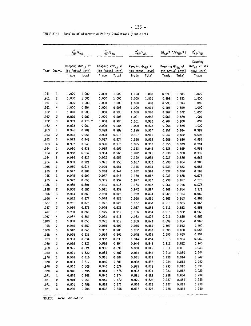
- 136 -
TABLE XI-1 Results of Alternative Policy Simulations (1961-1971)
KNAIKNA LNA/LNA KNA/KNA (WNA/P)*/(WNA/P) KNA/KNA
Keeping
Keeping W/PNA at Keeping W/PNA at Keeping eLNA at Keeping aLNA at W/PNA at its
Year Quart. its Actual Level its Actual Level its Actual Level its Actual Level 1964 Level
Trade Total Trade Total Trade Total Trade Total Trade
1961 1 1.000 1.000 1.000 1.000 1.000 1.000 0.996 0.893 1.000
1961 2 1.000 1.000 1.000 1.000 1.000 1.000 0.996 0.893 1.000
1961 3 1.000 1.000 1.000 1.000 1.000 1.000 0.996 0.893 1.000
1961 4 1.000 0.994 1.000 0.998 1.000 0.995 0.996 0.890 1.000
1962 1 1.000 0.988 1.000 0.996 1.000 0.990 0.967 0.872 1.000
1962 2 0.999 0.982 1.000 0.993 1.001 0.985 0.967 0.870 1.001
1962 3 0.999 0.976 - 1.000 0.990 1.001 0.980 0.967 0.868 1.001
1962 4 0.998 0.969 0.999 0.986 1.000 0.973 0.966 0.866 1.000
1963 1 0.996 0.962 0.999 0.982 0.998 0.967 0.957 0.884 0.999
1963 2 0.995 0.955 0.998 0.978 0.997 0.961 0.957 0.882 0.998
1963 3 0.993 0.948 0.997 0.974 0.996 0.955 0.956 0.880 0.996
1963 4 0.992 0.943 0.996 0.970 0.995 0.950 0.955 0.879 0.994
1964 1 0.990 0.938 0.995 0.966 0.993 0.945 0.938 0.869 0.993
1964 2 0.988 0.932 0.994 0.963 0.992 0.941 0.938 0.868 0.991
1964 3 0.986 0.927 0.993 0.959 0.990 0.936 0.937 0.866 0.989
1964 4 0.983 0.921 0.991 0.955 0.987 0.930 0.936 0.864 0.986
1965 1 0.980 0.914 0.990 0.951 0.985 0.924 0.938 0.882 0.983
1965 2 0.977 0.908 0.988 0.947 0.982 0.918 0.937 0.880 0.981
1965 3 0.975 0.902 0.987 0.943 0.980 0.912 0.937 0.878 0.978
1965 4 0.972 0.896 0.985 0.939 0.977 0.907 0.936 0.877 0.976
1966 1 0.969 0.891 0.983 0.936 0.974 0.902 0.964 0.916 0.973
1966 2 0.966 0.885 0.981 0.932 0.972 0.897 0.963 0.914 0.971
1966 3 0.963 0.880 0.980 0.928 0.969 0.893 0.963 0.913 0.969
1966 4 0.962 0.877 0.978 0.925 0.968 0.890 0.963 0.913 0.968
1967 1 0.961 0.875 0.977 0.923 0.967 0.888 0.913 0.863 0.968
1967 2 0.960 0.872 0.976 0.921 0.967 0.886 0.913 0.863 0.968
1967 3 0.958 0.869 0.975 0.919 0.966 0.884 0.913 0.862 0.968
1967 4 0.954 0.862 0.973 0.916 0.962 0.879 0.911 0.859 0.965
1968 1 0.950 0.856 0.971 0.912 0.959 0.873 0.899 0.864 0.962
1968 2 0.946 0.850 0.969 0.909 0.955 0.868 0.897 0.862 0.960
1968 3 0.942 0.845 0.967 0.905 0.952 0.863 0.896 0.860 0.958
1968 4 0.938 0.839 0.964 0.901 0.948 0.859 0.895 0.859 0.954
1969 1 0.933 0.834 0.962 0.898 0.944 0.854 0.913 0.884 0.951
1969 2 0.929 0.829 0.959 0.894 0.940 0.849 0.912 0.882 0.948
1969 3 0.925 0.824 0.956 0.891 0.936 0.845 0.911 0.881 0.946
1969 4 0.921 0.820 0.954 0.887 0.934 0.842 0.910 0.880 0.944
1970 1 0.918 0.816 0.951 0.884 0.931 0.839 0.935 0.914 0.942
1970 2 0.914 0.812 0.949 0.881 0.928 0.836 0.934 0.913 0.940
1970 3 0.910 0.808 0.946 0.879 0.925 0.832 0.933 0.912 0.939
1970 4 0.908 0.805 0.944 0.876 0.923 0.831 0.933 0.912 0.939
1971 1 0.906 0.803 0.942 0.874 0.921 0.829 0.938 0.884 0.939
1971 2 0.904 0.801 0.941 0.872 0.920 0.828 0.937 0.884 0.939
1971 3 0.901 0.798 0.939 0.871 0.918 0.826 0.937 0.883 0.939
1971 4 0.899 0.794 0.938 0.868 0.917 0.823 0.936 0.882 0.940
SOURCE: Model simulation

- 137 -
TABLE XI-2 Results of Alternative Policy Simulation (1976-1983)
KNA/KNA KNA/KNAKeeping W/Pna at Keeping W/Pna at
Year Quart. its Actual Level Year Quart. its Actual Level
1976 1 0.993 1980 1 1.0061976 2 0.986 1980 2 1.0081976 3 0.978 1980 3 1.0101976 4 0.971 1980 4 1.0111977 1 0.978 1981 1 1.0121977 2 0.985 1981 2 1.0131977 3 0.992 1981 3 1.0131977 4 0.998 1981 4 1.0141978 1 1.000 1982 1 1.0141978 2 1.003 1982 2 1.0151978 3 1.006 1982 3 1.0161978 4 1.008 1982 4 1.0171979 1 1.007 1983 1 1.0171979 2 1.007 1983 2 1.0171979 3 1.006 1983 3 1.0181979 4 1.005 1983 4 1.018
SOURCE: Model simulation

- 138 -
Appendix XII
MAIN INDICATORS FOR THE ECONOMY AND AGRICULTURAL SECTOR

TABLE Xll-l Real GDP and its Composition (1960-1984)
lear Real GOP Real GOP Share In Real GOP of ()("111 S 1971) Per Capita
(S 197J/person) Investment 1/ savtngs! lowports Exports
1960 187,100 25,372 14.6 10.7 2014 12.2
1965 196,048 IS.6 10.1 181.
1961 M0OM338 14.0 10.6 19.2 12.0
1963 zle,328 IS.? I.2 138.5 11.8
1964 223.186 18.5 15.1 20.1 12.7
1965 22'.990 11.9 16.4 19.S 12.5
1966 250.079 23.1 21.1 23.9 11.7
1967 256.598 20.3 18.2 21.0 11.?
1968 2?S,442 21.1 18.6 22.1 11.S
1969 271.393 22.0 21.1 24.3 1S.51970 283,097 31.863 23.4 21.6 24.0 11.S1971 3C9B.A 20.8 17.8 23.9 10.6
1972 30,70? 15.2 . 10.4 25.0 9.1
1973 287,7S0 14.3 9.S 25.0 9.9
5974 290,55' 25.8 25.3 25.6 14.3
197S 25.1CI. 14.0 I.S 18.0 16.9
1976 . 26I.94! 13.6 1S.4 18.2 20.2
1917 287.77G 14.4 10.7 22.4 20.6
5978 3lI11,' 16.5 11.6 24.4 21.2
1979 337,207 19.6 U-.7 27.6 22.3
1980 363,'46 23.9 IS.S 30.4 23.7
1981 M~.SSI 23.9 8.5 33.0 21.2?
1982 329,$23 29,192 9.6 2s.8 -27.5
1983 327,1E* 9.3 _ . 21.1l 25.2 '
1984 347.926* 1S.3- 24.3' 25.3
(* Estr-.ot avaf 'able.
1I Gross capital rori,ulon Total Gross Sav Cngs.NstGonal Grcss Savings a Yol GQss Savings - turrent Account Surplus.
SOURCtS: Central Bank of Chile 'IndIcddores EcorCIcosjy Socil.S, 1960-1982?Central Bank of Chile Bo tin HenTuiWy18f. TuiT9O iNational Bureau of Statistics.

TABLE Xll-2a Indices of Agricultural Output for Traded and Mon-Traded Products (1960-1984)
(1971 - 1976 * 100)* ~~~~~~Irport-Comcting (96 10
Year (1). (2) (3) (4t (61 ( )8 (1978 * Wheat maiz Ric* Sunflower Rapesed Sugar be"t Cattle mat Milk Total Imported
1960 31.S 51.3 1S4.2 273.3 50.7 33.2 70.1 79.1 80.01961 110.1 51.6 150.7 172.2 53.5 IS. 7S.3 80.6 70.31962 103.6 S.S 113.0 173.8 42.6 26.3 80.4 76.9 76.81963 121.3 S4.3 114.1 113.1 13.7 42.2 81.4 82.8 86.11964 123.8 16.8 11S.8 244.9 03.9 40.1 67.6 96.4 67.01965 119.2 82.7 1IS.7 24S.2 10.S 4I.S 69.8 64.3 81.01966 143.8 90.7 110.4 304.1 115.1 46.8 37.2 84.5 98.01961 121.6 11S.2 121.1 180.6 90.6 63.9 80.1 06.3 96.21968 12913 102.0 134.6 233.S 11.6 69.1 89.2 8a.0 98.31969 129.1 45.9 5?.8 153.1 94.9 6S.0 84.9 92.4 91.91970 139.6 76.0 101.7 151.1 104.4 100.9 89.1 93.1 103.41911 146.1 82.2 9F.6 110.4 122.6 84.8 77.S 91.8 102.S1972 121.1 90.0 124.2 108.0 116.3 13.3 60.0 91.5 91.81973 19.8 93.S 19.2 73.0 59.8 S2.2 45.4 6.9 68.1 I-
1974 100.3 136.S 49.5 56.6 S1.9 62.S 89.3 94.2 e6. -
191S 107.1 .10'.6 110.0 96.9 91.6 78.6 109.8 99.4 99.91916 92.6 t6.9 140.6 146.5 156.4 138.8 100.9 In6.3 100.0191 1'0.2 113.0 112.8 83.1 123.4 134.7 88.3 IC4.3 110.11978 35.3 81.7 150.9 363.1 71.6 5S.3 84.0 101.1 86.01979 106.3 ISS.6 2F0.8 180.1 96.4 41.4 85.3 99.2 97.51980 103.2 128.9 137.4 208.0 109.6 27.S 82.1 112.4 92.61981 73.3 164.8 143.6 40.4 40.1 89.1 9'.1 12'.8 93.41982 69.5 154.0 188.9 29.3 19.1 58.1 99.1 110.0 87.11983 62.5 162.7 166.5 25.0 4.2 100.2 106.0 93.6 86.81984 105.5 229.5 237.6 40.2 S.9 133.8 100.3 93.6 109.3

TABLE X11-Zb Indices ot Agricultural Output for Traded and Non-Traded Products (1960-1984)
Exported Non Traded
Year (10) (it) (12) (13) (14) (IS) (16) (17) (18) (19) (20) (21)
Apples Grappes Reach and Nectarines plums pears Dry beans Lentils- Onions Garlics Sheep meat lotalExportep(1976-100) Potatoes
(1974- 1976w100)
1960 8S.3 97.7 41.2 96.2 S9.0 104 160.4 - 144.3 118.8 - 103.5
1961 87.4 81.7 433 98.S 62.8 1OS.S 141.4 - 137.1 125.9 _ 110.S
1962 89.S 85.S 45.5 99.2 61.9 104.3 113.S - 146.2 120.0 - 100.3
1963 92.2 28.5 47.1 94.7 65.5 29.9 I13.S - lS5.0 121.8 - 111.1
1964 94.3 92.8 49.5 92.4 69.6 83.9 133.8 192.6 133.4 100.4 103.0 106.0
1965 81.3 VS.9 44.1 98.5 71.4 82.6 83.8 259.3 108.S 121.2 107.2 92.2
1966 - 9?.S 41.4 288.9 93.6 . 118.2 - . 10S2
19f - - - - - 12t.0 35.1 192.6 95.8 133.1 - a .
1968 . - - - - 91.3 36.0 150.0 104.7 158.0 - 94.9
1969 * - - - - 65.1 70.3 148.1 91.6 155.0 - 79.0
1910 126.6 - 99.9 214.3 314 92.0 100.9 136.9 18.7 133.1 - 89.6
191 - - - - - 101.3 108.1 133.3 96.6 147.9 109.6
1912 - - _ _ 1l6.3 96.4 92.6 91.1 9S.6 - 96.1
1913 9S.9 90.7 98.3 91.5 91.3 91.2 88.3 88.9 85.5 73.1 89.1 81.7
1974 96.1 96.8 10'.1 95.4 95.9 10S.0 115.3 100.0 O.S 96.2 99.2 132.6
1915 99.9 98.3 1C6.6 99.8 99.6 103.8 IC9.0 100.0 78.6 107.5 120.6 96.7
1976 103.9 104.8 89.3 304.7 104.6 .98.6 321.6 100.0 140.9 96.2 100.0 70.6
1917 119.9 144.6 91.3 111.9 IO.S 357.7 214.4 257.0 201.3 96.8 3t3.7 121.1
1978 139.9 125.5 86.1 119.9 112.4 157.3 1M1.2 238.9 201.3 96.8 14.3 128.S
1979 167.9 131.1 85.2 121.1 112.7 163.2 28s.6 233.2 201.3 105.1 1s6.7 101.0
3980 39S.9 141.4 83.7 128.5 11S.2 118.3 241.4 210.7 201.3 92.1 141.8 118.4
1981 238.5 202.S 80.9 130.3 122.3 194.1 IS9.5 240.1 100.6 92.7 . 170.3 132.0
1982 275.8 2?0.1 88.7 140.0 125.3 229.0 1'2.3 - - 64.8 - 110.3
1983 157.2 140.3 115.6 107.8 - 79.0 89.6
1984 .- 170.0 354.1 128.8 125.0 - 10.1 - 135.8
(-) not available.SOURCES: Column 1-1 15-16. 19. 21: National Iureau of Statistics (IW). Chile.
8 10-14 (1970-1924): Ag-icult.eral Bureau of Planning (COEPA), Chile.
8, 10-14 (1960-1965): 'Plan de Zesarrollo Frutfcols" (1;43) Production Development Corporation (CCRFO), Chile.
1/ Laspeyres phislcal production Indess. Basis: wkcleiale average prices for lmported and Eiported goods In 1976.

TABLE 111-3 Indices of Agricultural Food Production and Consumption
Year !jrIcultural Food Productfon Agricultural food ConsumptionYear
Total Per Capita Calories Index Proteins Index
(8Base 1974-7-l00) 10(Calories per (Base 72-74-100) (Crarres per day) (Base 72-74-100)1967 192J ~ r-,696-6 ;,zY 101.1 73.0 99.71968 96.5 109.81969 91.8 1OZ.4 1969-71 2.695 100.0 70.1 9S.81970 98.4 101.71971 96.5 103.51971 90.8 95.4 1972-14 2.694 100.0 73.2 JJ0.01973 85.0 87.81974 97.S 99.31915 103.2 .102.4 1975-71 2.644 98.1 70.3 96.01976 99.4 98.31977 107.0 10.S 19717-79 2.662 98.61978 98.4 93.01979 106.1 99.31980 106.1 98.3 1980-62 2.706 100.4 69.0 94.31981 113.1 103.5 . -.
' This figur' corresponds to 1982.Source: FAO Productilon Vear'och. Vols. ?2-36

TABLE 111-4 The Evolution of Governaent Revenues, Expenditures, Budget Deficit and Rate of Inflation (1960-1983)
Governrent Gcverncent Budget Share of Budget Deficit In Rate of Inflation AI)iYesr Revteues Expendftures Defkict totl T VailKI.ChT1 Cortailr-..HriiiiT
(A) (8) (C-9-A) Tudtat (BaP (se Cecewber 1978'100)(Thous. e each year) (--)--l oo (D) ge)
1960 707 907 199 2Z.0 4.? - -1.6 11.6
1961 B08 1I015 107 20.4 4.3 7.7 7.7
1962 959 1,277 318 24.9 S.6 13.9 13.9
1963 1,439 1,858 419 22.6 4.9 44.3 44.3
1964 2,123 2,647 S23 19.8 4.0 46.0 46.0
1965 3,a92 4.289 9 1 18.6 4.3 28.3 28.8
1966 5,247 6,046 199 13.2 3.0 22.9 22.9
.1967 6,.1)3 7,329 596 8.1 1.8 18.1 10.1
1968 9,163 9,996 833 8.3 1.8 26.6 26.6
1969 14,9es 15,506 SZI 3.4 0.8 30.7 30.7
1970 21,547 24,367 2.819 11.6 2.9 32.S 32.5
1971 25,510 31,571 1?,060 32.1 9.5 26.7 26.7
1902 '2,036 71,2SS 29,219 41.0 12.5 10.3 10.3
19'3 229,952 514,562 274,610 54.4 23.9 "13.7 '53.7 1
12t4 1.95'.Y46 2,61t?,370 857,423 30.5 9.3 513.1 491.2
19)5 8,975,471 lO,I71,4'l 1,201,9?9 11.8 3.4 377.8 380.1
1?.6 30.2QI.800 13316P."?7 2 266,251 8.9 2.3 210.7 2'1.7
1977 65,663.522 70e461.f?3 ,4798,361 6.8 1.7 91.7 114.3
I918 111.831,850 1 1!,°04.?68 A,067,106 3.5 0.8 40.2 49.9
1919 '89,295,360 176,550,200 -12,7A5,165 -7.2 -1.7 33.4 36.5
1980 218,16.600 24A,Z?S,100 -32.371,501 -13.1 -3.0 35.1 35.1
1981 310,322,700 31,P191.060 .22,137,643 -7.0 -1.7 19.1 19.1
198Z 318,36S,100 332,'03,500 13,938,401 4.2 1.0 9.9 9.9
1983 - - - - 27.3 Z7.3
30c4 , _ -
Average annual rate
Sources: Col. A,B,C: Banco Central (1983)Col. 0: National Bureau of Statistics and Yanez (1979)Col. E: CortArar and Marshall (1980)
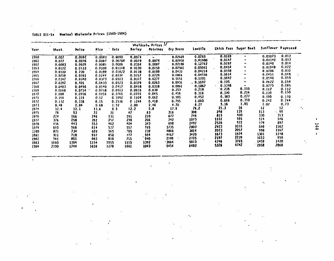
TABLE 1I1-5a Noouinal Wholesale Prices (1960-1984)
WUolisal. PrRtegTear llheat. %4b1s Pice Oats Barley Potatoes Dry SBans Lentils Chick Fess Sugar Beet Sunf1ower Rap?seed
1960 0.007 0.0082 0.0081 0.0090 0.0074 - 0.02669 0.0269 0.0169 - 0.01073 0.0121961 0.017 0.00?6 0.0047 0.007184 0.009 0.0074 0.02956 O.M1980 0.0141 - 0.01142 0.0131962 0.0083 0.00 9 0O8O o.cc86 o.0- 4 0.0087 0.02186 0.02762 0.0197 - o.ojo 0.0141963 0.0122 O.1Q33 0.0100 0.01148 0.0120 0.050 0.02501 O.OS061 0.0454 0.01948 0.0221964 0.0180 0.230 0.0189 0.01822 0.01;8 0.0188 0.0433 0.04214 0.0598 - 0.0286 0.032:965 0.0259 0.0261 0.0244 0.0234 0.0257 0.0220 0.0866 0.04596 0.0614 - O.C451 0.0481966 0.0347 0.0340 0.03t3 0.0S13 0.0317 0.0277 0.I051 0.1201 0.0941 - 0.0540 0.0591967 0.0392 0.401 0.0433 0.0523 0.0319 0.0263 0.0931 . 0.1697 .0.105 - 0.0622 0.CS4:968 0.0483 0.0496 0.05*0 0.0431 0.0418 0.0318 0.0861 0.1867 0.1396 - 0.0775 O.C853369 O.0668 0.0754 0.0738 0.0513 0.0655 0.030 O.2S3 0.218 0.238 0.155 0.112 0.112j970 0.088 0.C956 0.0956 0.I005 0.03SS 0.04S 0.459 0.316 0.3)0 0.214 0.139 0.1501911 0.106 0.119 0.32 0.3092 0.1104 0.062 0.50S 0.452 0.383 0.277 0.190 0.1701912 0.13Z 0.338 0.15 0.2536 0 i244 0.418 0.795 1.060 0.666 0.359 0.242 0.2441913 0.48 2.84 0.68 3.92 2.00 2.46 4.70 6.27 5.16 1.81 1.07 0.731974 12.4 12.1 13.6 8.5 12.2 5.8 17.9 ?6.2 21.3 16 12 121975 78 53 72 31 47 63 336 308 248 135 I13 .991976 224 166 246 131 191 210 877 749 635 400 330 3131977 316 258 392 257 2I8 206 742 1073 1122 595 524 5461918 t96 443 553 462 404 342 698 2497 2526 !22 !79 897 I1319 650 566 614 527 557 765 1135 2803 2923 ICSS 660 1162:?0 821 7134 689 SG5 05 739 4806 3814 2023 2057 998 11671981 911 718 987 85a /t1 594 44t67 3420 16713 1974 1301 12181982 961 801 883 830 7 .5 940 2189 2105 . 2197 2239 1C53 9501983 3660 1384 1154 lOSS II1S 1392 *3604 S033 4746 3765 1459 )4201984 ?DO0 1744 1659 1270 1661 1043 5454 6483 5326 4742 2858 2868

TABLE III-Sib No1eal Wholesale Prices (1960-1984)
Year Live Cattle Plg Heat Chicken Nen eggs Cow m1lk fresh Wool Siples Grapes
In carcass$/sa ,/ia ~~t1v9 ILI°o u 1. _ t , 1/1oo kg$ ; /100 tqs -
1960 0.- 350.052 ~ Obi 6ZMpFr B.d8 r05§ -- 0.00731
1961 0.A 0369 . O.0O'.659 0. 04 0.0000648 0.dO081 0.0161S - OOIC98
1962 0. INV4lI 0.000744 - 0.204 0.000079 0.00107 0.00E4S 0.01160
1963 0.000638 0.001040 - 0.006 0.000106 0.00208 0.0108 0.016501964 0 0O01 0.001544 - 0.008 0.000134 0.00310 0.0165 - 0.01680
1965 0.00144 0.00206 - 0.012 0.000209 0.00351 O.GIU .0.02400
1966 0.0018 0.00269 - 0.012 0. 00£W2 0.0039 0.0253 0.031S
19E] 0.0213 0.00406 - 0.018 0.00C:08 0.0043 0."S'2 C.066
ISEU 0i.e274 O.O494 - 0.24 O.eOe496 0.0G466 0.06t) 0.1021
19f.9 0.00197 0.00(J8 - 0.A3S O.OO66 0.0067 0.102 0.1464
19)0 0.0S07 0.00911 - 0.5S 0.00047 0.0092 0.161 0.2095
1971 0.0)e47 0.0128S 0.Q6 0.0M326 0.011 0.154 0.2010
1972 .0'129 0.01973 O.IS 0.0014S 0.022 0.329 0.353
1973 0.C886 0.1077 0.15 0.89 0.0135 0.14 2.365 2.94
1974 0.798 0.S958 0.99 3.35 0.0978 0.90 9.186 21.09 . _
1975 1.3 2.33 3.72 15.81 0.423 2.81 82.1 36.9 4
1976 7t 5 11.14 14.15 60.9e 1.34 !!.75 221.9 118.S (7
1977 17. 0 32.22 29.08 loe.iS 2. I .i.37 571.0 360.2
1978 2?6' t41.25 39.19 130.e 4.'38 49.87 549.8 52e.4
1979 40.60 5%.)? 54.er 204.44 S.97 6e.27 663.0 677.5
1980 51.80 76.28 56.29 ?nf.31 7.47 79.)8 925.8 1034.5
19el 49.88 82.03 57.0S 212.53 7.01 69.88 921.4 1,022.9
2962 6. 5S 77.91 54.21 25S.00 8.43 S7.39 832.1 693.0
19e3 S7.19 10.52 82.12 3P6.13 11.65 99.9S 1,038.6 714.7
1984 83.39 137.52 112.37 *eo.00 16.03 159.00 2,02S.9 98(.8
I/ All fig9et are expressed In new pesos'
()Informatior. nct*wV411tle.SOURCES: 1960-1968: indicadores Agroeconimtcos H1, Agricultural Planring Office. Ministry of Agriculture. Chile.
1969-1.92: 4atlonal Bureau of Statistics, Chile.19713-19el: IN( (National Dure.u of Statlitics). Chile.

TABLE X11-6a Nominal Constmer Prices (1960-1904)
Tear Dread 3/ Edible 011 Rice Sugar Cry Beans Potatoes Fasteruvled Pcidi.(S/g. ) ($/Lt.) (S/Kg.) (S/Kg.) (S/Kg,) ($/Kg.) (M/Lt) (S/Lk*
1960196119621963 0.00029 0.0010' 0.00049 0.0005l O.00Q39 0.e0017 0.00014 0.012411964 0.0cc41 0.00138 0.00053 O.OOC8S 0.OOCSS *0.00026 -0.00019 0.002971965 0.0053 0.00194 0.00074 O.OOC8S 0.00096 0.00030 0.00028 0.004481966 0.00065 O.0025 O.OoC86 0.00094 0.00108 0.00037 0.00035 0.05%61967 0.00074 O.0z29 0.0010S 0.00118 0.00116 0.00035 0.Q0042 0.06E751968 0.vi Ce 0.00404 0.OPi 31 0.00176 0.00131 0.00044 0.30052 0.008951969 0.0Q109 0.00558 0.00183 O.00232 0.00205 0.00048 0.000651910 0.00300 1Z 0.00135 o.e.os5 0.00320 0.00315 0.00071 Q.00083 0.01508 Y1911 0.00270 0.00825 0.ooues 0.00391 tL110498 O.O0O0 0.00130 0.015631912 O.00455 0.011252 0.00461 0.00803 o.Ce853 0.00E14 0.00233 0.010951973 0.01681 0.07966 0.05£930 0.03727 0.05354 0.C&20 0.01065 0.W4122074 0.2256 0.999 0.$604 0.525 0.2!482 0.C98 0.1130 2.0201915 1.24 4.24 2.410 2.61 3.80 0.770 V.6600 9.11421916 3.11 15.50 6.10 5.01 10.10 2._4 2.35 21.681917 6.57 27.67 9.18 1751 13.36 '.39 5.42 £6.691?.8 20.85 40.21 17.70 12.94 10.48 5.10 8.90 75.781'79 :6.15 51.?e )?.44 16.9 36.00 9.95 12.19 139.8015?0 20.98 56.82 22.41 31.43 63.30 10.09 16.35 18.23919P1 24.20 55.36 28.14 31.02 65.34 10.13 19.65 158.281?Q$ 29.61 65.51 29.46 24.53 35.03 13.88 21.09 158.54I'83 '0.11 91.64 39.10 34.73 52.51 19.54 27.97 238.9819°4 46.32 141.41 S0.50 40.24 78.79 15.78 35.09 316.31

TABLE XII-6b Nominal Consumr Prices (1960-1984)
Sutter Ch,!Se Cattle Chlic&a lien rggs Wine Beer Apple% Grapes
(t/rg.) (I/Kg.) (S/Kg.) (1(100) (SIlt.) (liLt.) (1/Kt.) (i/kg.)
1960I 6119621961 0.00297 0.00751 0.0M62 0.0013S 0.00041 O.OOOSI -
1964 0.004?2 0.00318 O.0033 0.00059 0.00062 0.00076 -
1765 O.OC656 0.0'516 0.014 0.00093 0.00076 0.00111 -
191;6 O.C0O24 0.008S 0.020 0.00105 0.00094 0OOIS9 -
1967 0.00343 0.01013 0.023 0.00121 0.00120 0.0018 -
1968 0.01145 0.01418 0.030 0.00170 0.06163 0.00221
1969 0.01508 O.MI16. 0.0427 - - 0.00391 9
190 0.01941 0.02649 0.011es O .C'o 0.00os9 - 0.004 sl -
1971 0.02012 0.0349? 0.0l3S1 0.0750 0.00619 - O.0S23 -
19Q2 0.C269 0.C9?2I O.fic2S 2.19 0.01329 - 0.01772 -
1971 0.326M0 0.51?SI O.IM948 0.136 0.1114 - 0.08011 -
1974 3.242 2.331 0.')fl0 0.386 M.SISS - 0.35
1975 11.87 10.76 4-sS 2.10 2.070 .. 14 0.67
1975 32.01 30.21 16.04 10.16 3.47 3.21 2.79
1977 53.36 57.S3 33.10 129.41 1.08 8.77 6.05
1978 84.22 9(-54 46.J7 174.33 , 11.23 11.90 6.51
1979 10.79 142.30 60.SS 269.00 17.24 15.18 10.32
1980 134.07 186.67 63.10 30'.08 22.26 20.10 18.70
1981 167.51 187.81. 65.13 31^.50 29.39 26.09 15.82
19e2 209.C1 19e.?O 62.31 356.5 31.38 27.31 10.33
19P3 289.77 256.27 91.06 531.33 37.66 32.73 16.9C
1984 361.80 325.20 126.70 S56.25 46.08 25.88 22.26
I/ All nu-ters are ex;ressed 1n new pesos".7/ Since .13-"-y 1°?0 a e price series Is used.1/ 0trIn5 the per!ods 15.-191C and 19?4-194 the price correupcnds to an average of several types of broad. In
1271-73 orl 1 ore type of bread 1 produce4.4/ The price represcnts, during 1960-1970. an over3ge of two types of mil1k.
SOURCE: Natlonal Bureau of Statistics (IE). Chile.

TABLE 111-7a Agricultural Production (1260-198i4)
. ar& WIttat Nil*e Rice Oats Brley Potatoas Ory Beans Lentils Chick Feat Sugar Beat Sunflower
(thousand tons)
1960 13,43.6 161.0 10.1 90.1 as'.? 790.0 13.8 17.8 3.3 544.1 S0.)1961 1,030.5 162.8 .N4.7 101.S 71.9 6'2.9 15.2 13.7 3.1 251.4 .31.11 9?69. 180.8 78.5 81.8 73.3 M65.3 74.3 12.6 3.1 430.6 32.0
1961 1)135.6 176.0 71.3 93.7 96.7 847.6 64.1 12.6 3.2 692.3 32.01964 1,158.8 241.5 80.5 85.8 80.4 8308.4 64.1 13.3 3.1 658.1 4*.11965 1.115.8 259.9 .:80.4 82.2 74.0 -03.2 58.9 9.3 S.1 680.6 45.21966 1,346.4 285.3 76.7 107.4 88.0 803.0 68.8 4.6 4.9 167.6 56.01967 1,203.4 362 2 84.2 115.2 117.5 716.6 89.8 3.9 8.0 14047.9 33.3968 1 215.8 320.8 93.5 1 8.4 156.9 124.1 65.1 4.0 7.7 1j152.6 43.0 4
1969 1,214.2 153.8 36.7 95.2 60:1 602.S 46.8 7.8 3.5 1 DS5.9 28.21970 1,306.9 239.0 76.2 110.5 91.4 683.1 6S.6 11.2 5.4 19655.1 28.2197 1 1,36.9 2S8.3 61.1 112.0 113.6 83-.1 12.2 12.0 7.2 12390.7 20.33972 11195.1 283.0 86.3 111.] 139.0 733.0 82.9 10.7 9.3 1,201.6 19.91971 ?16.6 294.0 54.9 109.1 I07.4 623.6 M.0 9.8 4.1 856.0 13.51914 Si9.0 3669. 34.1 149.9 141.6 1,012.0 14.8 12.8 S.0 1 025.3 10.49795 I Oc3.0 328.9 76.4 11.1 1490.6 131.9 74.0 12.1 4.9 1:616.1 17.8
3976 ^e66.4 247.9 91.6 95.9 e9.0 538.9 10.3 13.5 2.1 236.2 21.01917 1,2:9.3 355.1 120.0 123.1 143.1 9e.4 112.4 21.8 S.0 2 208.4 15.3971 t;92.6 256.9 104.8 92.7 1?5.5 ;80.1 112.1 19.0 S.5 840.3 30.1
:919 995.1 c89.3 181.2 150.2 112.1 710.S Il6.3 33.1 9.4 6 9.S 33.3l9eo 966.0 405.2 95.4 112.6 105.0 90.1 84.3 26.8 11.6 450.2 38.319bl 685.9 SlE2 99.7 130.6 91.i 1.001.3 338.3 17.1 6.4 1,460.4 7.41962 650.4 454.1 131.2 117.6 111.8 041.6 12.5 35.8 4.1 961.0 4.41983 585.0 511.5 315.6 146.3 13.2 683.6 84.4 13.8 3.9 19642.5 4.61984 988.0 721.4 165.0 163.0 MS3 15036.2 94.1 16.0 6.9 2,193.9 1.4

TAltE 111 - Jb g picultural Production ({1960-1)
Tear Rapeseed graps Apples etae - Pears Plus CattleMt Milk PigMeat SheepMtNearine in Carcass (NIllItons Lts 4 In In Carcass
.-47- .V . *ons Carcass
(thn4and tons)
1960 34.0 46.7 106.9 S6.4 20.0 12.7 136.7 760.4 360.6 .1.5 Z0.0
1961 3S.6 49.1 109.S S9.3 21.3 13.0 141.5 775.1 321.8 28.9 21.2
1962 25.6 -S.4 112.1 62.3 21.0 13.1 157.8 739.2 375.2 24.9 20.2
1963 49.4 S3.2 115.5 64.5 2?.2 12.S 159.8 194.2 *32.1 25.4 20.S
2?64 56.2 S5.6 118.2 67.7 23.6 12.2 132.7 R'0.S . 441.6 27.1 16.9
1*6S 72.0 S7.8. 101.1 61.2 13.1 13,1 137.0 810.2 415.8 3Z.5 20.4
1966 77.1 - - - . . - ISI.4 -12.0 415.1 34.4 19.9
1967 .- 60.7 - - - - 1S7.3 129.1 439.2 36.6 22.4
1968 47.9 - - - - 172.2 V:S.7 476.4 41.6 26.6
1969 63.6 - - - , - 166.7 PTA.6 519.4 *2.2 26.1
1910 69.9 - 160.8 136.7 38.t 28.3 176.1 895.1 525.9 44.4 22.4
1971 82.2 - - 152.1 940.0 S71.2 45.2 24.9
1972 77.9 - - - - 117.8 seO.0 506.4 S5.4 16.1
1973 40.0 S4.5 120.0 134.6 31.0 12.1 eq.2 ?55.0 441.7 49.2 13.3
1974 34.6 S0.2 120.8 1'2.S 32.S 12.6 115.2 905.8 522.8 49.9 16.2
197S 68.4 S9.1 - 125.0 145. 33.8 13.2 215.4 9S6.0 579.9 29.9w1 18.3
1976 104.8 63.0 130.0 122.3 3S.S 13.9 19e.2 1,021.0 593.9 24.9 15.2
1977 82.7 68.9 150.0 125.0 37.5 14.8 173.3 1 103.0 607.7 28.9 16.3
1978 52.0 75.4 175.0 117.8 38.2 15.8 164.8 977.9 557.0 33.9 IS.1
1979 64.6 78.9 210.0 116.6 3e.3 16.0 167.4 953.S S19.1 42.5 17.7.
1980 72.4 M50 24S.C '114.5 39.1 11.0 162.3 I1,00.0 592.2 49.7 IS.5
1981 26.7 121.? 298.4 110.7 11.5 17.2 18'.6 I3,?'.0 SS3.1 55.8 15.6
1982 13.2 .162.4 345.0 121.3. 42.6 18.4 194.6 1.S86.0 S67.1 45.0 10.9
3')53 2.9 196.0 365.0 136.0 47.6 .8 208.1 gn. 502.1 59.3 13.3
4.1 225.0. 410.0* 1'0.0- 52.3. 22.5. 196.8 00.0 *91.5 59.1 11.9
*roPvstonal figures.(- No Informatfon available.
SOURCE: National !ureau of Statistics, Chile. Agricultural Sureau of Planning, Chile.
Plan Racional de Oesarrollo rrutfcola (1968)

Distributors of World Bank PublicationsARGENTINA FINLAND MALAYSIA Forsaobotr arilemCanon Hirsch SRL Akateerinen Kirjakaupp Univerriy of Malaya Cooparahvo International Sbaiopton Sfviet,Gateria Guem. P.O. Bo 128 Bfoekhep, Limited P.O. B.o 41D95Florida 165,4th Pl eOfoc 453/465 SF0101 P.O. Bo 1127, Jlal Pnbta Sra, Craighall1333 Bueno Aires Hdelk 10 Kuala Lumpw Joumnesbun 2D24
AUSTRAUA,PAPUANEW GUINEA, FRANCE MEdiCO SPAINF[ILSOLOMONISLANDS, Wsdd Bank Publicatin lNFCOTEC Mundi-Prenra Libro, SAVANUATU, AND WESTERN SAMOA 66, avenue d'lra Apartado Postal 22-260 Ctedlo 37DA. Bo.iko&oJourna 75116 Paris 14060Obt1pmn MedooDE. 2(DI Madrid
11-13St.ator BteetMitcham 3132 GERMANY, FEDERAL REPUSUC OF MOROCCO Litberfa ntInadonal AEDOSVidona UNO-Va1lg Soceted EtudseManketing Marocaine Conaeilde Cent 391
Popprsdcl.fe, A2eeSS 12 rueMozartBd d'Anf* CN9BacelnnaAUSTRLk D-m Bon I CasablancaGerold and Co SRI LANKA AND THE MALDIVESGraben 31 GREECE NETHERLANDS Lake HoumeBookhopA-1011Wien KEME InOr-Pulibv P.O. Boo 244
24, Ippodamou Sbet Plada Platiras PIO. Box 14 10D, Sir Chittampalam A. GardinerBAH'RAIN Athess,11635 7240 BALoLhn MaseathaBahrann Research and Coniuany Cdombo 2
Aasodats Ltd. GLATEMALA NEW ZEALANDP.O Box 22103 Ubeerias Ptedra Santa Hill LUibrary and IonoraahonSmvice SWEDENManama Town 317 Centro Culturil Piedra Santa Privategag Frsixgkeitle
11 calle 6-50 ztona I New Market FPitao FPkbokaoroetsBANGLADESH Guatemala Clty Auddand Regernoggatw 12 Sox 16356Micro lndutirs Devdeopment S-103 27StodhoIm
Asslitanc Socety CMiDAS) HONG XONG, MACAO NlGERIAHoumeS, Road 16 Aa 20 Ltd. Univesity Prom limited Fwbaoip os efaDhanmondi R/Area Manglak Post OffIe Three Ce. BlduifdtogJetjdn WsrnenWilltaaAS9Dhaka 1209 BueSteBetNo. 37 PrivatemallBag50 S BDo 304
Ma.gkoI, Kosioon Ibrdan S104- 2 StockholmaBmIf oan i:rs: Hong Kog1536 NurAhmed Sarak NORWAY SWITZERLANDChittagn,g 4X00 HUNGARY Narvesenln aitdon Cenrer FwoAgletitlan
Kularsa geetrandNarvsenotvei2 UibeisiePayot76, KDA. Aene PO. Bo 139 P.O. Bo 6125 Etttad 6,rue,GeenKulna 139 Budapet Q N-0602 Olo 6 Case pol 3i1
CHi1211 Genea BELGIUM INDIA OMANPublicatrono dea Nations Unies Allied PubEthees Privae Ltd. MEMRB IIofrmation SMorts Forubsoritre oeiemA. du Ro 202 751 Mount Road P.O. Boo 1611, SffoAirport UbtairiePyot1060rua- Madras -600092 Muscat SertioedosAborneamenot
Case pot 3312BRAZIL BSchJfIka PAKISTAN CHICD2 LausannePublicacoes Teoicas Internadconal 15 JN. HosediA Marg Mirsa Saok Agency
Ltda Ballrd EBlte 65, Shahhe-Quaid-Aurm TANZANIARua Peixoto Gomide 2D9 Bombay - 40 038 P.O. Bo No. 729 Oxfod Unitrdsity Press31409Sw0 Pauo., SP Lahore3 PfO. Box 529
13/14Asaf Al Road Dure SalaamCANADA NewDdhi -110(D2 PERUD,eDiffusr Ediosia DesasoIo SA THAiLAND
C.P, 65,1M1mrue Arnp,e 17ChittaranjanAvenue Apaado 3824 Central Deptrment StoreBouch-ville, Quebec Calcutta 70D072 Lintk 356 Siln RoadJ4B 5s6 Bangkok
Isyadeva Hostel Buiding PHiLIPPINESCHINA 5th Main Road Gandhintagar Nasosal Book Stcr TRtNIDAD & TOBAGO, ANTIGUAChina Pinan,dal JY Eoanomro Publiohing Bangaloe 560109 701 Etoal Avenue BARBUDA, BARBADOS,
Homse P.O. Bo. 1934 DO MINICA, GiERNAD A. G-UYANA,S, Da Po Si DcngJie 3-5-112 Kacddguda Cross Road Metro Manila JAMAICA, MONTSERRAT, ST.Beijing Hyderabad - SW 027 rITTS & NEVIS, ST. LUCiA
POLAND ST. VINCENT 6,GSRNAOINESCOLOMBIA Prarthana Fat. 2nd Ploor ORPAN Sylmatits Studies UnitEnlaceL da. NeArThakwesBau&Navrangpura Pawc Kulhtuy iN.ui 9 Watst StreetApartadoAnreo34270 Ahnmedabad -i3O009 0-D901 Wrova CurepeP,ogota OE. Trinidad, West Indies
Pataa Housae PORTUGALCOSTA RICA 16-A Aahok Marg ULvoart Patugai TURKEYUbrciaToejos Lwscknof 226C01 Ru Do Caimno7-76 Had eKiapv AS.Callell-13 12 Lisbon IStikbal Cadder No. 469Av. Pernande. Gueti INDONESIA BeyogluSan Jose Pt Indir ULmited SAUDI ARABIA, QATAR Istanbul
JL Sm Ratulahog 37 lairtrBookSteenCOTE OPDVOIRE P.O. Box 11 P.O. Box 3196 UGANDACentre d'Editns et de Diffsion. Jakarta Pumat Riyadh 11471 Uganda Bookahop
Afr1oaines (CEDA) P.O. Boo 714504 S.P 541 IRLAND MEMRB Information Seevic KampalaAbidjan 04 Plateau TDC Publisess BraCAri
12 Noth Fredertck Street AlAl.a Street UNITED ARAB EMIRATESCYPRUS Dublin I Al Dahoa Center MEMRB Gulf Co.MEMRBi formadon Sicv e First Floor P.O. Boo 6097P.O. BEo 3155 ITALY P.O. Box 7188 S2arjahNicosit LF cos Comutoainarata Sran SPA Rtiyadh
Via Besedeto FornI, 120/10 UNITED KINGDOMDENMARK Casetd Pbotale 552 Haji Abdullash Alra Building Migoinfo Ltd.Sa-fundsLtttratur 51125 Florense King Khlaed Street P.O. Bo. 3RaoenooemrnAi1 1 P.O. Box 3969 Alto., Hampthire GU34 2PGDK-197D l'red.ai1kbosg C JAPAN Dorman England
Easten Rook SrviceDOMINICAN REPUBUC 3743 Hango 3-Chone., unkyo-ka 113 33, Mohanoned Hasaan Aood Street URUGUAYEdttor Tale, C. por A. Tokyo PO. Boo 5978 Instituto Naronsal dd LibroRestaurasdon e babel la Catolica 3K Jeddah San Jose 1116Apotado Post 2190 KENYA MonettidleSanto Dormngo Africa Book Service (EA.) Ltd. SINGAPORE, TAIWAN, MYANMAR,
P.O. Box 45245 BRUNEI VENEZUELAEL SALVADOR Nairobi Inmion Publcatior Ubreria del EsteFusades Privatb Ltd Aptdo. 603t7Avenida Manuel EnriqueArauj. 13530 XOREA. REPUBUC OF 02-06 1st FL Pei-Fu Induooial Caracas 1060-AEdifido SISA, le. Pla Pa Katit Book Coipwatiicn BidgSan Salvador P.O. Boo 101. Kwsng,hmun 24NewfudustrtalRoad YUGOSLAVIA
Senoa Stngapoe 1953 Jugoalovenmka KnjigaEGYPT, ARAB REPUBLIC OF YU-I110CD Belgrade To5 RepublikeAl Ahram KUWAIT SOUTH AFRICA, BOTSWANAAl Caiaa Stret MEMRB Informatton Seevi-os Fwwisr titiiaCairo P.O. Boo 5465 ODford Univer tly Press Southern
TheMiddle East Ooerer P.O. Box 1141S Chiawarot Street Cape Tonwn 8iJCairo


The World Bank
Headquarters European Office Tokyo Office1818 H Street, N.W. 66 avenue d'lena Kokusai BuildingWashington, D.C. 20433, U.S.A. 75116 Paris, France 1-1 Marunouchi 3-chome
Telephone: (202) 477-1234 Telephone: (1) 40.69.30.00 Chiyoda-ku, Tokyo 100, JapanFacsimile: (202) 477-6391 Facsimile: (1) 47.20.19.66 Telephone: (3) 214-5001Telex: WUI 64145 WORLDBANK Telex: 842-620628 Facsimile: (3) 214-3657
RCA 248423 WORLDBK Telex: 781-26838Cable Address: INTBAFRAD
WASHINGTONDC
0-8213-1453-X