anca cristea david nber - world...
TRANSCRIPT
Estimating the Gains from Liberalizing Services Trade: The Case of Passenger Aviation
Anca CristeaUniversity of Oregon
David Hummels Purdue University, NBER
Brian RobersonPurdue University
May 2012

Liberalization and services trade• We know relatively little about how services trade is
affected by efforts at liberalization. Why?
• Measurement:– Service trade data are highly aggregated; values, not P and Q
• Policy change is difficult to quantity– Literature relies on cross country comparisons, and existing
rules are complex.– Service trade lib. occurs along with other domestic reforms, and
technological change (e.g. finance, telecomm). – E.g. Contrast cutting tariff on Mexican steel ball bearings from
15 to 5% with guaranteeing “market access in business services”
2

We focus on passenger aviation. Why?
• International passenger aviation is important– Big (US + EU = $190bn/year)– A key input into
• merchandise trade (Poole 2009, Cristea 2011)• knowledge flows (Hovhannisyan and Keller 2011), • Other services (GATS mode 2, mode 4)
• Not obvious that liberalization will generate benefits– Liberalization may result in consolidation/collusion– Distribution of gains may be uneven
• The data are a thing of beauty.
3
Data on aviation and policy change
• We have a nice policy experiment: – From 1992‐2007, the US signs 87 bilateral “Open Skies Agreements” that liberalize trade in passenger aviation.
• We have detailed firm‐level transactions data on US passenger aviation, 1993‐2008.– Prices, quantities, routes offered, carriers competing for precisely defined services
• e.g. coach ticket from IND ‐> ORD ‐> CPH
4
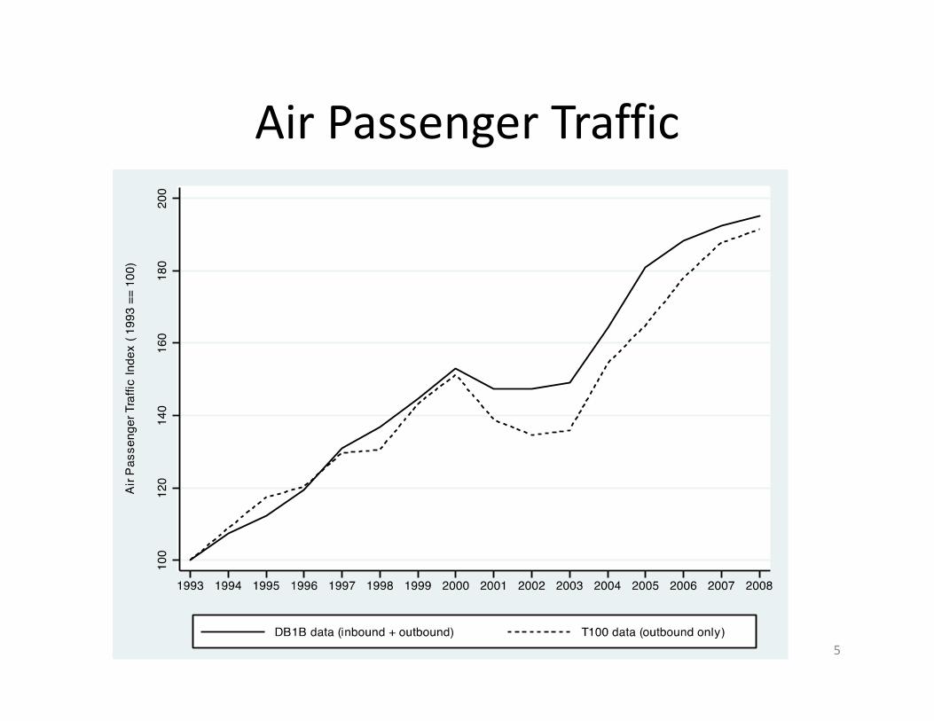
Air Passenger Traffic
5

Trends in Airfares
6
Dotted line: US BTS price index (Fisher)‐ exact match of ticket
Solid line: all DB1B data; estimate perioddummies including “true” origin‐dest FE

Past Regulatory Regime
• Chicago Convention (1944): failed attempt to set multilateral agreements on air services
• Countries negotiated air service agreements (ASA) on a bilateral basis. These are typically characterized by– Market access restrictions
• pre‐defined points of origin and destination– Limits on entry and capacity
• fixed number of designated airlines and limited flights – Price control:
• advance double‐approval for all airfares
7

Eg: US‐China Aviation Treaty 1980• Only 2 carriers per country can offer service
• Flights allowed only between– LA, SF, NY, Honolulu– Beijing, Shanghai– Tokyo is only 3rd country city from which airlines can operate in
serving market
• Carriers can offer two flights per week for a given route
• Price changes must be submitted to DC, Beijing for approval two months in advance.
8

Bilateral Open Skies Agreements
• Remove most existing restrictions– No limit on carriers, routes, capacity– Price setting at carriers discretion
• Grant new benefits– Extensive “beyond” market rights– Allow inter‐airline cooperation agreements
• Alliances, code‐shares
9

10
CopenhagenChicago
RomeIndianapolis
Gateway to gateway
beyond

Timing of open skies agreements
11
Agreements are signed sequentially; order weakly correlated with GDP
Europe spread throughout sample.
NZ 1997, Australia 2008
See Table A1
DemarkSweden
PortugalFrance UK, SpainItaly
Germany

Model (quick sketch)• Multiple carriers serving each country pair
– Each carrier has preferred “low cost” city, can offer service out of other cities, but at higher cost
• E.g. Delta prefers Atlanta…but could fly Newark.• Carriers differ in which cities are low cost
• Two‐stage game– One: firms commit to aggregate capacity (# planes)– Two: firms allocate capacity to city pairs and play Cournot.
• Extension of Anderson‐Fischer (1989) multi‐market oligopoly to case of multiple heterogeneous firms and markets.
• Examine outcomes (p, q, markups, # routes & carriers) in two cases– Post‐OSA. Entry into all cities is permitted.– Pre‐OSA. Entry allowed in subset of permitted cities.
12
Carrier entry under route restrictions
• cp, carriers prefer to allocate capacity to low cost locations
• With pre‐OSA route restrictions, two things can happen. – Carriers with high cost on permitted routes devote low capacity
or stay out of city market entirely, reducing competition; or– These carriers enter permitted routes, and increase
competition, but industry average cost of service goes up
• Eliminating route restrictions allows carriers to sort on cost– Capacity constraint encourages reallocation of planes away from
high cost routes permitted pre‐OSA• Some routes see entry of carriers, others see exit
– Industry average cost drops.
13
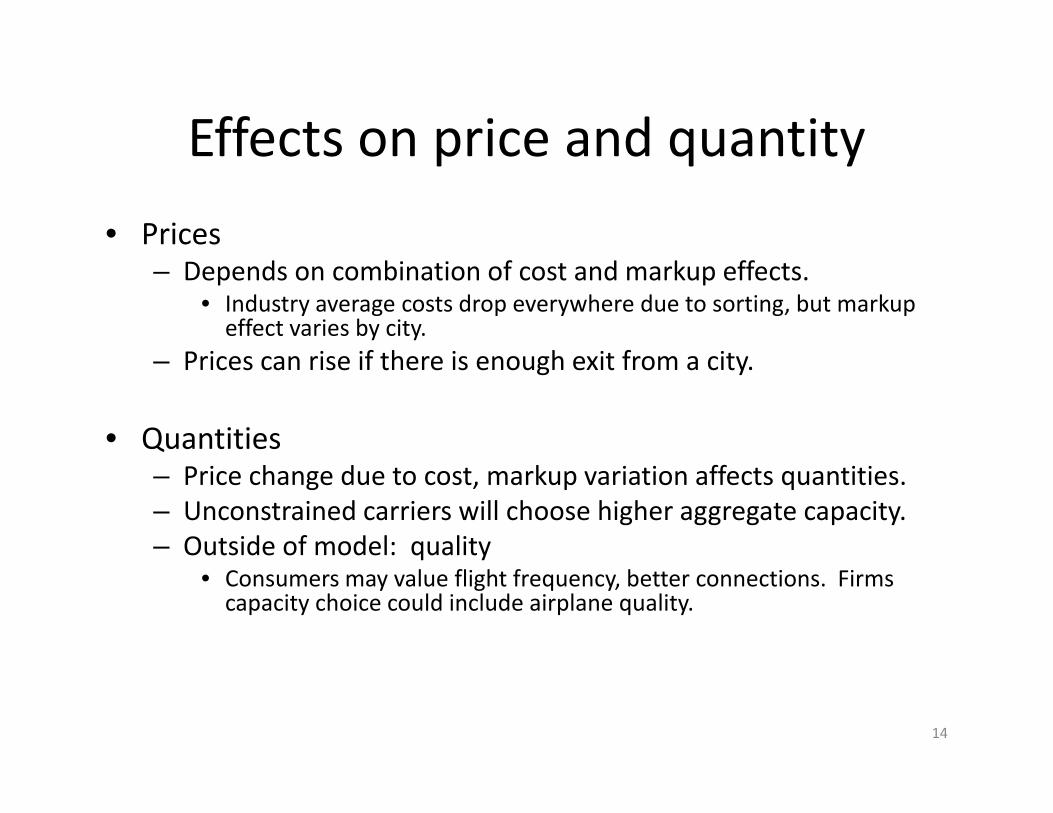
Effects on price and quantity• Prices
– Depends on combination of cost and markup effects.• Industry average costs drop everywhere due to sorting, but markup effect varies by city.
– Prices can rise if there is enough exit from a city.
• Quantities– Price change due to cost, markup variation affects quantities.– Unconstrained carriers will choose higher aggregate capacity.– Outside of model: quality
• Consumers may value flight frequency, better connections. Firms capacity choice could include airplane quality.
14

Other Restrictions (future work) • Advanced notification of price changes
– difficult for carriers to manage yields (capacity utilization) if demand is uncertain.
– planes fly with empty seats despite MC ‐> 0, and the passengers who would fly if price dropped.
• Restrictions on alliances and code‐shares– A core rationale for “national” service providers is to prevent
monopolization by foreigners– Relaxing restrictions may allow carriers to realize comparative
advantage on routes, and increase capacity utilization– or, allow them to pursue anti‐competitive market share
agreements.
15

Does OSA liberalization lead to welfare gains?
• Its not obvious. • Provisions in OSA could
– raise or lower prices by affecting average cost of entrants and/or markups
– raise or lower quantities sold by• Affecting prices• Changing the set of routes on offer• Affecting service quality (quantity net of prices)
– affect the distribution of gains• Redistribute them between carriers and consumers• Redistribute them away from consumers on permitted routes and toward consumers on not permitted routes
16
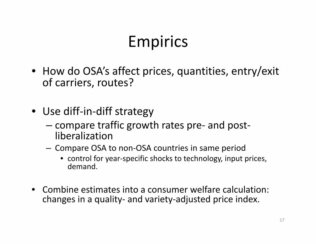
Empirics
• How do OSA’s affect prices, quantities, entry/exit of carriers, routes?
• Use diff‐in‐diff strategy– compare traffic growth rates pre‐ and post‐liberalization
– Compare OSA to non‐OSA countries in same period• control for year‐specific shocks to technology, input prices, demand.
• Combine estimates into a consumer welfare calculation: changes in a quality‐ and variety‐adjusted price index.
17

Timing of open skies agreements
18
Agreements are signed sequentially; order weakly correlated with GDP
Europe spread throughout sample.
NZ 1997, Australia 2008
See Table A1
DemarkSweden
PortugalFrance UK, SpainItaly
Germany
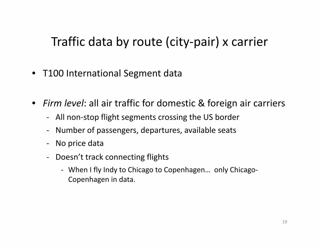
Traffic data by route (city‐pair) x carrier
• T100 International Segment data
• Firm level: all air traffic for domestic & foreign air carriers‐ All non‐stop flight segments crossing the US border‐ Number of passengers, departures, available seats‐ No price data‐ Doesn’t track connecting flights
‐ When I fly Indy to Chicago to Copenhagen… only Chicago‐Copenhagen in data.
19

Price and Quantity Data
• Origin‐Destination Passenger Survey
• Transaction data: 10% sample of int’l airline tickets – air fare paid– service characteristics (dist, # segments, transit airports, class)
– all segments of the itinerary and carrier(s)• Many tickets involve joint production of several carriers
– Does not cover “non‐immunized carriers”
20
Air Passenger Traffic
21
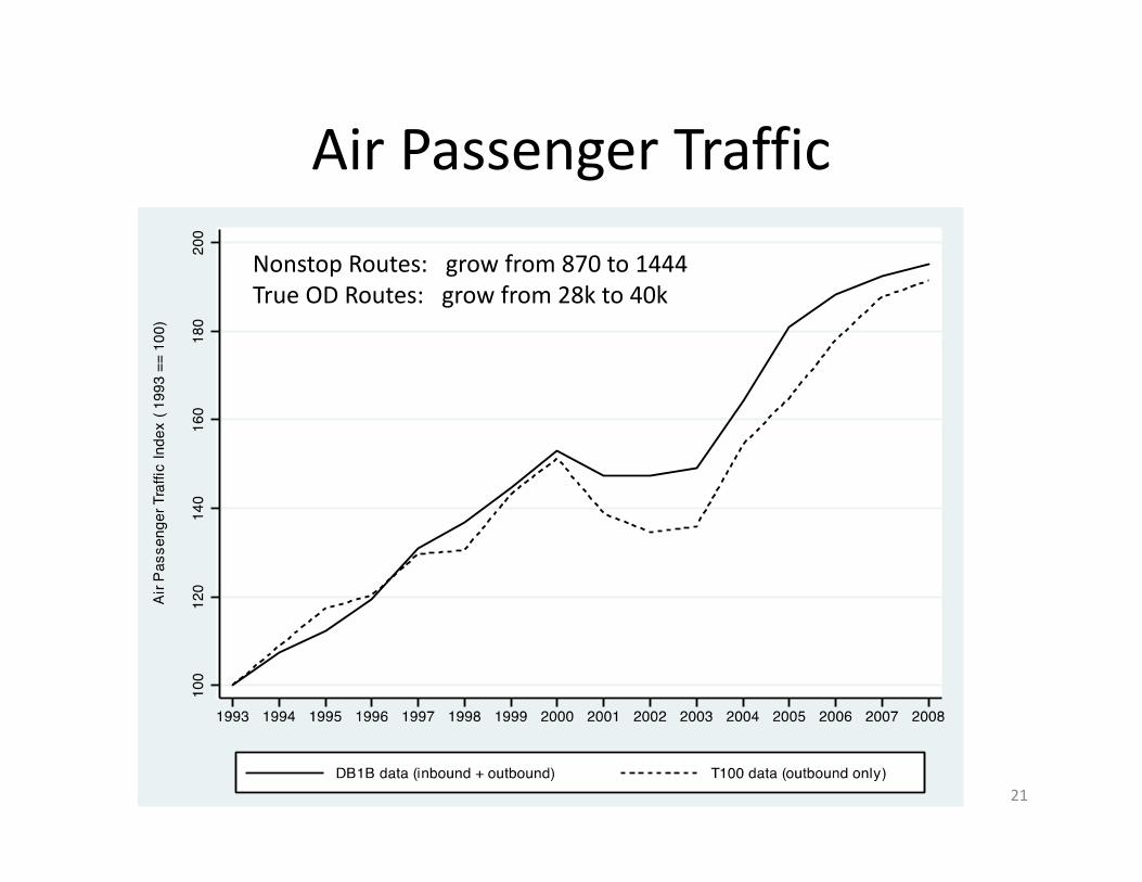
Nonstop Routes: grow from 870 to 1444True OD Routes: grow from 28k to 40k

Estimate the impact of OSA on traffic
Difference‐in‐difference estimation method for the number of U.S. passengers abroad:
Z is growth (relative to 1993) in a measure of passenger traffic
22
9393 93, 1 , 2 3 , ,,
ln ln / lnj t j t j t jq t j tj tZ OSA Y L L X
Index j = country, q = qtr t = year

Estimate the impact of OSA on traffic
Difference‐in‐difference estimation method for the number of U.S. passengers abroad:
23
9393 93, 1 , 2 3 , ,,
ln ln / lnj t j t j t jq t j tj tZ OSA Y L L X
Country x quarter FE: allow differences in traffic for country j – season q
Income, population growth: absorb change in traffic demand for country j
Year effects: absorb common cost shocks, trend growth in air travel;

Estimate the impact of OSA on traffic
Difference‐in‐difference estimation method for the number of U.S. passengers abroad:
To pick up effect of OSA• Dummy: OSA = 1 for any year that agreement is in effect• Interact OSA dummy with vector D(‐3) to D(+5) for the age of the OSA agreement
allows us to identify pre‐existing trends, lagged effects of signing
24
9393 93, 1 , 2 3 , ,,
ln ln / lnj t j t j t jq t j tj tZ OSA Y L L X

25
Total traffic

Open Skies and Traffic Growth
26
Traffic Share covered by Open Skies (%) Cumulative Growth (%)
1993 2000 2008 Total Passengers
Non-Stop Routes
True O&D Routes
Nafta 0 0.0 53.2 102.5 122.6 27.6
Latin America & Caribbean 0 28.5 41.0 93.9 85.5 40.8
OECD Europe 7.7 43.3 100.0 76.0 12.4 36.5
Europe & Central Asia 0 37.0 60.4 245.2 53.8 205.4
Southeast Asia & Pacific 0 22.2 32.6 38.8 8.2 49.4
Middle East & N. Africa 0 8.9 7.1 102.2 16.7 -1.4
TOTAL 79.4 66.0 109.1

Decompose changes in trafficWrite:
Intensive margin = air traffic on existing city‐pair routes (continuing service)
Extensive margin = flight service on routes never offered before1. simple counts of routes2. Passenger weighted counts of routes (in manner of Feenstra 1994)
based on t‐3 weights.3. Could also count carriers as distinct “varieties”
(United and Delta flights from Indy‐> CPH are different services)
Replace Z in estimating equation with components above
Recall: pre‐existing bilateral ASAs specifically restrict entry to particular routes, carriers
27
1 1 1effect effect
on the EM on the IM
* EM IMjt jt jt
OSA OSA
Q EM IM

28
Total traffic
Growth in New Routes
Traffic on Existing Routes
Extensive margin is much larger when using simple counts, much smaller if we use route x carriers
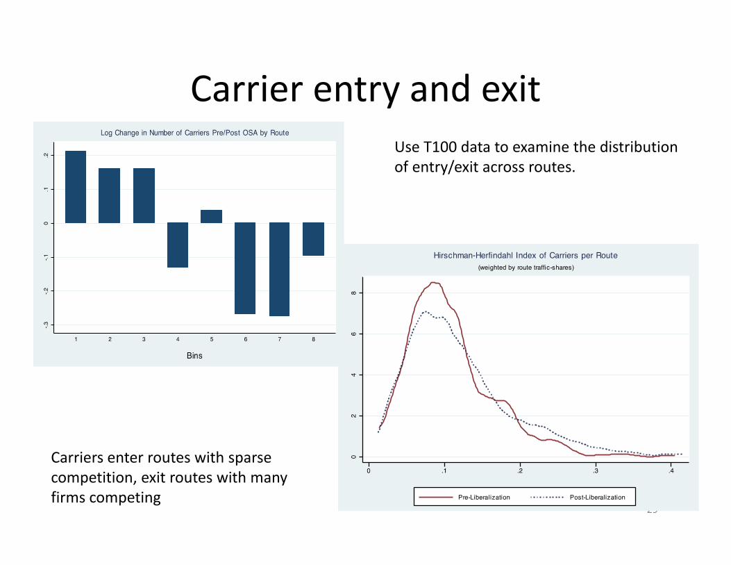
Carrier entry and exit
29
Carriers enter routes with sparse competition, exit routes with many firms competing
Use T100 data to examine the distributionof entry/exit across routes.

Understanding the channels
• OSA could raise or lower prices– Reduced unit costs from rationalized operations, economies of route density; and lower markups generated by net entry
– Consolidation creates collusion, higher markups
• Conditional on prices, OSA could raise or lower quantities by changing service quality– Flight frequency, connectivity, use of preferred carriers– Reduced incentive for firms to compete by overinvesting in quality
30

Estimating price equation• Use O‐D ticket data to estimate changes in prices for a
given “true” origin‐destination route r.
• Starting from about 40 million tickets: Aggregate all tickets within a given route r at time t– We might have 10 different ways to get from Indy to CPH, on many different carriers
– We create a (passenger weighted) average price for route r, from country j, time t.
• Use diff‐in‐diff: how do average prices on OSA routes change relative to non‐OSA routes?
31

32
MelbourneSF
Sydney
IndianapolisLAX
All possible routings to get from IND to MEL are aggregated for a given year, but we keep track of average characteristics (distance, number of segments)

Controls in price equation• Cost shocks
– Control for route FE, ticket characteristics (distance, number of segments) – rjt varying
– Economies of route density (population & number of possible destinations reached by each airport)
– Include time FE (costs common to all routes in a time period)– Route‐time varying cost shocks (fuel*dist, insurance*geographic
region)
• Include OSA, and OSA connect dummy – OSA: direct effect on traffic originating/terminating in OSA ctry– OSA connect: indirect effects for traffic connecting through an
OSA country but originating or terminating elsewhere• E.g. fly through Denmark to get to Italy.
33
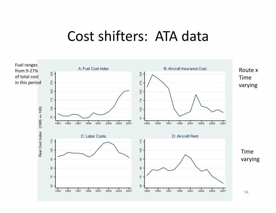
Cost shifters: ATA data
34
Time varying
Route xTime varying
Fuel rangesfrom 9‐27%of total costin this period

Price Regressions: (DB1B)
35
Dependent variable: Economy Class Airfare (log)
(1) (2)
OSA 0.004 -0.015***[0.005] [0.005]
OSA Connect * Distance Share -0.105***[0.009]
OSA * Share US Origin (outbound)
No. Connections (log) 0.238*** 0.243***[0.008] [0.008]
Observations 599,533 599,533R-squared 0.203 0.204
Control Variables:
Cost shifters:Ticket DistanceFuel*Distance
Aircraft Insurance*World Region
Trip characteristics:One‐way
Avg. Number of ConnectionsOutbound
Traffic Density:US state Population
Foreign Country PopulationTotal Departures at Origin
Total Departures at DestinationTotal Direct Routes (country)
Other:Partial Liberalization

Entry and exit
36
Carriers enter routes with sparse competition, exit routes with many firms competing
Use T100 data to examine the distributionof entry/exit across routes.

Price effects by entry/exit(outbound)
37
Dependent variable Economy Class Airfare (log)All Routes Net Exit Net Entry
OLS OLS OLS
OSA -0.001 0.043*** -0.023***[0.007] [0.008] [0.007]
Economy Class Fare
Observations 545,345 433,592 480,365R-squared 0.056 0.057 0.053
Sample: only tickets that match gateway‐gateway routes; outbound flows only

Estimating Quantity equation• Use O‐D ticket data to estimate changes in demand on a given “true” origin‐destination pair “r”.– More general than T‐100, has all segments and all destinations (not just gateways); can control for prices
– Include all tickets with same origin‐destination
• Prices instrumented with fuel*distance, insurance costs*region interactions
• Demand shifters: – Population, income; bilateral trade; number of segments– OSA variable measures increase in traffic conditional on prices, other demand shifters.
38

39
Dependent variable: Number of Air Passengers OLS 2SLS
(1) (2) (3) (4)
Economy Class Airfare (log) -0.068*** -0.067*** -1.412*** -1.412***
[0.007] [0.007] [0.112] [0.112]OSA 0.048*** 0.088*** 0.062*** 0.002
[0.011] [0.012] [0.011] [0.015]OSA Connect 0.099*** 0.077*** 0.083***
[0.008] [0.009] [0.009]
OSA*US origin share (outbound) 0.107***
[0.015]No. Segments (log) -1.255*** -1.269*** -1.269*** -0.930***
[0.033] [0.033] [0.033] [.049]Observations 599,619 599,619 599,606 599,520R-squared 0.228 0.228 --First Stage Statistics:F-Test of iv 112.2 108.2Hansen's j stat 146.3 126.6
Quantity Regressions (DB1B)
Instruments for Airfare:Ticket DistanceFuel*Distance
Insurance*World Region
Control Variables:
Trip characteristics:Direct (non‐stop)
Avg. Number of ConnectionsOutbound
Market size:US State Population
US State IncomeForeign Country Population
Foreign Country IncomeTotal Exports
Total Direct Routes (country)
Other:Partial Liberalization
Caribbean Trend

40
Dependent variable: Number of Air Passengers OLS 2SLS
(1) (2) (3) (4)
Economy Class Airfare (log) -0.068*** -0.067*** -1.412*** -1.412***
[0.007] [0.007] [0.112] [0.112]OSA 0.048*** 0.088*** 0.062*** 0.002
[0.011] [0.012] [0.011] [0.015]OSA Connect 0.099*** 0.077*** 0.083***
[0.008] [0.009] [0.009]
OSA*US origin share (outbound) 0.107***
[0.015]No. Segments (log) -1.255*** -1.269*** -1.269*** -0.930***
[0.033] [0.033] [0.033] [.049]Observations 599,619 599,619 599,606 599,520R-squared 0.228 0.228 --First Stage Statistics:F-Test of iv 112.2 108.2Hansen's j stat 146.3 126.6
Quantity Regressions (DB1B)
Instruments for Airfare:Ticket DistanceFuel*Distance
Insurance*World Region
Control Variables:
Trip characteristics:Direct (non‐stop)
Avg. Number of ConnectionsOutbound
Market size:US State Population
US State IncomeForeign Country Population
Foreign Country IncomeTotal Exports
Total Direct Routes (country)
Other:Partial Liberalization
Caribbean Trend

D(qty) as a quality effect
• OSA’s improve flight frequency, connectivity, use of preferred carriers; may also induce competition through better amenities on planes.
• To extract this…
41
ln ln where rjt rjt rjt rjt rjt rjt jt rjtq E p X OSA
OSA quality effect (price equivalent) = / .107 /1.4 7.6%
This attributes none of other sources of quality change (e.g. reducing number of flight segments) to the OSA

Welfare calculation
To measure OSA relative to non‐OSA, we capture1. Relative price movements from OSA price regression2. Construct quality adjusted prices by netting off the effects of
OSA on “quality” (measured as OSA effect on quantity net of prices from quantity regressions.)
2. Use quality adjusted prices to form relative price series; then apply Feenstra 1994 to get variety adjusted price index
42
1/( 1)
1
tt t
t
P
Pt
pit
pit1
iwit
r
ir iri Ir
ir iri I
p xp x
Variety adjusted price index Price index for
common setVariety adjustment

Applying this to the policy experiment
43
Sigma estimated using either variation across routes
OSA direct OSA connect
Sigma == 1.25 outbound inbound outbound inbound
D Airfare (price effect) 0.000 -0.026 -0.060 -0.053
D Quality (quantity effect net of prices) -0.098 -0.038 -0.102 -0.102
D Quality Adjusted Price Index 0.902 0.936 0.839 0.846
D Lambda-ratio Variety Index 0.755 0.755 0.755 0.755
D Variety Adjusted Price Index 0.681 0.706 0.633 0.638
Drop in Price Index due to OSA (%) 31.91% 29.41% 36.70% 36.18%
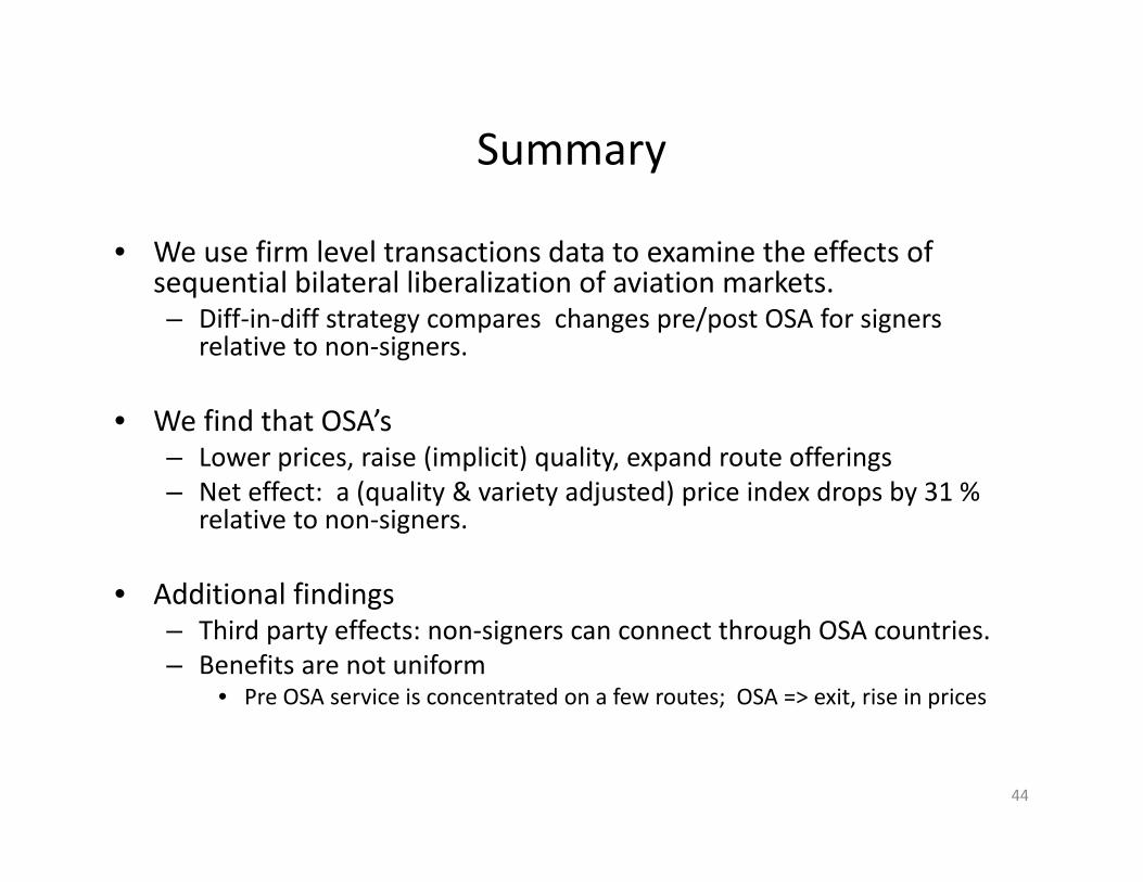
Summary
• We use firm level transactions data to examine the effects of sequential bilateral liberalization of aviation markets.– Diff‐in‐diff strategy compares changes pre/post OSA for signers
relative to non‐signers.
• We find that OSA’s– Lower prices, raise (implicit) quality, expand route offerings– Net effect: a (quality & variety adjusted) price index drops by 31 %
relative to non‐signers.
• Additional findings– Third party effects: non‐signers can connect through OSA countries.– Benefits are not uniform
• Pre OSA service is concentrated on a few routes; OSA => exit, rise in prices
44

Supporting slides
45

Understanding the quantity channels
• Conditional on prices, OSA raise quantities.– Relax capacity constraints– Raise service quality
• To examine first channel, measure the extent of capacity constraints– Load factor = passengers / seats– How high was load factor pre‐OSA? – Did load factor change as a result of OSA?
46

Is D(qty) due to relaxed capacity constraint?
• Pre‐OSA Load factor never exceeds 85%. Median 63.6%• Load factors rise post‐OSA.
– Elasticity of load factor wrt OSA = 0.026.
47
Organize routes into 8 bins by pre‐OSA load factors.
Number is max load factor in that bin
Height of bar is log change in passengers post‐OSA

Aside: load factors and prices
• Suppose – carriers enter a route until P = AC– conditional on making a flight, marginal cost of a passenger is very small.
• Then: – AC = cost of a flight/number of passengers– This is the inverse of the load factor
48
ln ln load factor .026ln ln
POSA OSA