1

This draft: December, 2010

TRADE COSTS AND ECONOMIC DEVELOPMENT

Michele Fratianni Indiana University Kelley School of Business 10th and Fee Lane, Bloomington, Indiana 47405 (USA), and Università Politecnica delle Marche, Ancona (Italy) email: fratiann@indiana.edu

Francesco Marchionne* Università Politecnica delle Marche Facoltà di Economia ‘Giogio Fuà’ Piazzale Martelli, 8 60121, Ancona (Italy) email: f.marchionne@univpm.it.

* Corresponding author. We are indebted for comments and suggestions to Pietro Alessandrini, Davide Castellani, Jack Lucchetti, Chang Hoon Oh, Alberto Zazzaro, various participants at the annual meetings of the Italian Economic Association and seminars at the Universities of Ancona, Naples-Parthenope, Molise and Urbino.

2

TRADE COSTS AND ECONOMIC DEVELOPMENT

Abstract

We test the hypothesis of the circular causality between trade costs and degree of economic development using data on Italian provinces. Using different methods to control for multilateral resistance, we apply a gravity equation to estimate sectoral exports to 188 countries over the period 1995-2004. Provincial trade costs are constructed as the sum of five province-specific elasticities, including distance, adjacency, and common money. We find that Italian provinces are heterogeneous with respect to trade costs. These costs are influenced by lagged provincial per capita income and industrial structure. In turn, trade costs influence future provincial per capita income. This two-way relationship between trade costs and income is broadly consistent with the cumulative causation process emphasized by the New Economic Geography. Key Words: trade costs, heterogeneity, economic development, gravity equation. JEL Classification: F10, F14, O52, R12.

I. INTRODUCTION In this paper we test the hypothesis of the circular causality between trade costs (TCs) and degree of

economic development using data on Italian provinces. This bi-directional causality is a typical

implication of New Economic Geography (NEG) models but, to our knowledge, it has not been

tested before. To motivate our hypothesis, we draw on the link between TCs and cross-border trade

flows and the link between TCs and spatial economic disparities.

There is ample evidence that TCs play an important role in international trade. A decline in

international transportation costs, a component of TCs, is a likely cause underlying the sharp rise of

world trade relative to world output that has occurred over the last fifty years (Hummels, 2007).

Transportation costs rise with distance and, consequently, close countries tend to trade more than

distant countries. Trade-enhancing characteristics that counteract transportation costs are: common

language (Helliwell, 1999; Hutchinson, 2002), common colonial roots (Rauch, 1999), shared

religion (Kang and Fratianni, 2006), immigrant links to the home country (Gould, 1994; Head and

3

Ries, 1998) or more generally ethnic networks (Rauch and Trindade, 2001), and similarity in

economic development (Fratianni and Kang, 2006). Beyond culture, cross-border trade is

influenced by institutions such as regional trade agreements (Carrère, 2006; Baier and Bergstrand,

2009) and common money (Rose, 2000; Rose and van Wincoop, 2001; Frankel and Rose, 2002).

Last but not least, national borders are a big impediment to trade (McCallum, 1995; Helliwell,

1998; Anderson and van Wincoop, 2003; Chen, 2004). Behrens et al. (2007) break down the

complex range of TCs in a transportation component and a non-transportation component (e.g.,

border-related impediments and differences in languages and in monies). These authors find that the

former impacts on the location of firms whereas the latter exerts a global impact. In their extensive

survey, Anderson and van Wincoop (2004, 691-2; AvW henceforth) estimate that TCs represent the

equivalent of a 170 percent ad-valorem tax barrier to trade, of which 21 percent attributable to

transportation costs, 44 percent to border-related impediments, and 55 percent to distribution costs.

In sum, TCs are large and complex. An often cited paper by Obstfeld and Rogoff (2000) argues that

TCs are the common cause to six major puzzles in international macroeconomics.

TCs are also critical in NEG, which is concerned with the spatial distribution of production

facilities and agglomeration factors. Krugman (1991), the leader of NEG, develops a core-periphery

model that hinges critically on the interaction of transportation costs with scale economies in

production.1 The model features a sector, agriculture, with constant returns to scale and an

immobile factor of production, land, and another sector, manufacturing, with increasing returns to

scale and a mobile factor, labor. Pecuniary spillovers trigger a “circular causation” process whereby

manufacturing tends to concentrate in locations with large markets that, in turn, lead to more

concentration because those locations enjoy lower effective prices and attract mobile labor. The

outcome is the endogenous formation of a richer industrial core and a poorer agricultural periphery,

or more generally regional economic disparities. The income differences result from differences in

prices, with workers in the core enjoying higher real wages than in the periphery. Agglomeration

accentuates as transportation costs decline, giving more incentive to footloose manufacturing to

1 On this point, see the survey article by Head and Mayer (2004).

4

relocate. Agglomeration can also arise through cost and demand linkages stemming from firms

using intermediate goods (Venables, 1996) or through innovation (Martin and Ottaviano, 2001).

The spatial distribution of industrial activities and income is affected critically by TCs.

When TCs are high, interregional trade is low and industrial activities are widely diffused. As TCs

decline, agglomeration, with its attendant benefits of increasing returns and external economies,

develops in core areas (what is core is largely a path-dependent process). Agglomeration is fed by

the industrial sector drawing the mobile factor, say labor. If labor is mobile only between sectors in

the same region, the agglomeration process reaches a turning point when real wage differentials are

sufficiently high to induce firms to relocate from the high-wage agglomerated region to the low-

wage non-agglomerated region. In this case, periods of industrial concentration are followed by

periods of a more even spatial distribution of industrial activities (Puga 1999; Bosker et al. 2007).

The spatial distribution of per capita income will also mimic such a pattern. If labor is instead

mobile among regions, the agglomeration process in the core region will continue until real returns

on labor are equalized across regions. In this case, the spatial distribution of industrial activities

remains asymmetric and regional economic development is heterogeneous. In sum, causality runs

from TCs to agglomeration and income. But there is also the opposite causality from agglomeration

to TCs. The core attracts firms and labor from the periphery because it enjoys higher productivity,

including sectors such as information services and distribution that are so important for

international and interregional trade. Scale economies from agglomeration reduce TCs. The core

also benefits from better infrastructure and public administration resulting from agglomeration,

which tend to reduce TCs. In the end, causality is potentially bi-directional.

To test our hypothesis, we follow a two-step approach. First, we estimate provincial TCs

using a gravity equation (GE) applied to bilateral trade flows from the viewpoint of a country, Italy,

that shares common culture and national institutions, but suffers from regional disparities. Second,

we test the mentioned two-way causality between provincial TCs and provincial per capita income,

our measure of economic development. While Italy is not the only industrial country with regional

disparities, its heterogeneity is long dated: the Mezzogiorno problem, or the relative low degree of

5

economic development of the Italian South, goes back to the creation of the nation in 1861 and has

defied decades of large government transfers from the North to the South over the last fifty years.

Much has been written on the subject both inside and outside Italy; space permits only a few

references. Lutz (1962) is among the first to analyze in depth the Italian dual economy, which exists

not only geographically but also across industries. Her policy prescription is wage flexibility in the

South and interregional mobility of labor and capital. Chenery (1962, 515) examines the policy of

the Italian government “to carry out the theoretically attractive procedure of developing external

economies by a massive dose of public works while leaving the direct investment in commodity

production to private individuals.” This policy has continued to these days despite the persistence of

the North-South economic divide. Labor mobility across regions remains relatively low (Mocetti

and Porello, 2010), a fact that is difficult to reconcile with the gap in per capita income. The twin

occurrence of large geographic economic differences and labor immobility remains an “empirical

puzzle” (Faini et al. 1997).

The literature on regional disparities has gone beyond the North-South characterization. For

example, Bagnasco (1977) identifies three distinct economic areas: an old capital-intensive North-

West, which he calls First Italy; an agricultural and backward South, which he calls Second Italy;

and a newer North-East and parts of the Center, which he calls Third Italy. Third Italy is replete

with dynamic small and medium size firms that outsource production and are located in industrial

districts (Brusco, 1990). These districts specialize in different products and are distinctive in their

development paths, local institutions, and manners of generating externalities (Becattini, 1990,

2007).2

The paper is organized as follows. In Section II, we discuss the general form of GE in the

presence of multilateral TCs. In Section III, we formulate the empirical equations of our two-step

approach. Section IV discusses the data. Section V presents and analyzes the findings. Section VI

deals with robustness tests. Conclusions are drawn in the last section.

2 Markusen (1996) discusses different types of industrial districts (agglomeration).

6

II. THE GRAVITY EQUATION AND MULTILATERAL TRADE COS TS

In a well-known paper, McCallum (1995) applied a GE to 1988 exports and imports among ten

Canadian provinces and thirty U.S. states and found that inter-provincial trade was approximately

twenty times larger than trade between provinces and states; in essence, the US-Canadian border is

very thick. AvW (2003) criticized McCallum’s findings mostly for ignoring multilateral TCs and

argued that general-equilibrium considerations dictate that trade flows from region i to region j

depend, among other factors, not only on bilateral TCs, but also on multilateral ones.3 When

multilateral costs rise relative to bilateral costs, trade flows rise between i and j. These authors

derive the following operational GE (see their equation 13):

σ−

⋅⋅

=1

ji

ij

w

jiij PP

t

Y

YYX , (1)

where X = exports from i to j, Y = nominal income, t = bilateral TC factor, P = multilateral TC

factor (i.e., consumer price index), σ = elasticity of substitution among goods, and i, j, and w

indicate, respectively, exporter country, importer country and the world. Assuming that tij is a

function of bilateral distance and one plus the tariff-equivalent bilateral border barrier, AvW

estimate with nonlinear least squares a simultaneous system of equations on cross-section data.

Their main result is that borders reduce trade in the range of 20 to 50 percent, that is much less than

the border found by McCallum.

The AvW estimation procedure is rather cumbersome and other authors have sought simpler

alternatives. Baier and Bergstrand (2009) obtain virtually identical results with bonus vetus (good

old) ordinary least square (OLS, henceforth) using a first-order log-linear Taylor series expansion to

approximate multilateral resistance with appropriate exogenous variables captured by country fixed

effects (FE henceforth). Following Rose and van Wincoop (2001), Feenstra (2003), and Cheng and

Wall (2003), Baldwin and Taglioni (2006) instead propose time-invariant country-specific dummies

3 The immediate predecessor of AvW is Anderson (1979). Other theoretical foundations of GE are provided by Bergstrand (1985, 1989), Deardorff (1998), Helpman (1987), and Haveman and Hummels (2004).

7

for cross-section data and time-varying country dummies and country-pair FE for panel data. In

panel data, the time-varying country dummies remove the time-series correlation and the country-

pair FE the cross-sectional correlation. However, country-pair dummies (simply, pair dummies) are

time-invariant and consequently can only in part account for the multilateral resistance factor; serial

correlation remains. There are two downsides to this procedure. The first is that it involves a great

number of dummies and the estimation depends on sample size. The second is that pair dummies

capture all FEs, including distance elasticity, and consequently make it impossible to distinguish

among parameters of various time-invariant variables. The alternative to the second downside is

provided by Carrère (2006) who models pair dummies as random variables (RE henceforth). By

employing pair REs, we can still apply the Baldwin and Taglioni’s approach to handle the

multilateral resistance factor, but in addition we can estimate the impact of distance on trade

(Fratianni et al. 2010).

III. EMPIRICAL SPECIFICATION OF THE TWO-STEP APPROA CH

We discuss in this section the empirical procedure and econometric methodology underlying the

two-step approach. In the first part, we focus on the construction of provincial TCs. These are the

sum of five components: distance, adjacency, common and different regional trade agreements, and

common money. In the second part, we lay out the model of circular causation between provincial

TCs and provincial per capita income.

Step 1: Gravity equation and provincial trade costs

The specification of TCs is the subject of theoretical and empirical debate; see, for example,

Fingleton and McCann (2007). Bosker and Garretsen (2007) discuss and estimate various

specification of TCs and conclude in favor of the “implied TC” specification (see their equation 16).

Since our data do not permit such an estimation, we follow the trade literature in defining TCs in a

8

multiplicative form.4 Specifically, the TC of the kth product exported by the Italian ith province to

the jth importer country is given by (see Carrère, 2006):

][ 43210 ijjtjtjt ADJACENCYMONEYInterRTARTAijijt edt

ρρρρρ +++⋅= , (2)

where dij is bilateral distance, RTA (InterRTA) is a dummy that assumes 1 (0) when i and j belong to

the same (different) regional trade agreement, MONEY and ADJACENCY are dummies that assume

1 when i and j share the same money or a common land border.5 Institutional and cultural factors

such as common language, colonial relationships and immigrant links are irrelevant in the Italian

context and have been omitted.6 As to the signs of the coefficients, ρ0 is positive and ρ3 and ρ4 are

negative. The signs of ρ1 and ρ2, instead, depend on whether the RTA is trade creating or trade

diverting. If the RTA is trade creating, both ρ1 and ρ2 are negative; if the RTA is trade diverting ρ1 is

negative but ρ2 is positive (Carrère, 2006). A RTA could evolve over time from a trade-creating to a

trade-diverting institution (Fratianni and Oh, 2009).

Substituting (2) in (1), we obtain a testable GE at the provincial level that is similar to AvW’s

(2003) equation 19:

ijtf

ijtfijjtitijt fZdYYAX ερσρσ +−+−+++= ∑=

4

10 )()1(ln)1(lnlnln , (3)

where ( )σσ −−= 11ln jtitw

t PPYA is the multilateral resistance factor, Yi and Yj are respectively nominal

income of i and j, and Z(f) is the set of four variables that affects TC in addition to distance:

Z1=RTA, Z2=InterRTA, Z3=MONEY, and Z4=ADJACENCY. Distance elasticity 00 )1( ρσβ −= is

negative since the elasticity of substitution σ is larger than unity; the four semi-elasticities

ff ρσβ )1( −= are positive, except for β2 < 0 when the RTA is trade diverting; εijt is an

idiosyncratic error. 4 The implied TC specification requires data on total consumption of goods only produced by the province. Since we lack inter-provincial trade flows, we cannot implement this procedure. 5 All Italian provinces share the same regional trade agreements and currency. While RTA, InterRTA, and MONEY have a global impact, their provincial export elasticities can differ due to different frequencies of these three factors in each province. Sixteen Italian provinces are adjacent to either France, Switzerland, Austria, and Slovenia. 6 Italian, as the majority’s language, is only spoken in Italy. Colonial relationships with former colonies Libya, Somalia and Eritrea were too short lived to be of any relevance. Emigrants’ relationships are primarily with the home country. Furthermore, these relationships have diminished over time and are captured in our model by importer country FE.

9

Sectoral distance elasticities are estimated under the restriction that these elasticities are

common to all provinces (a restriction imposed by data availability). Provincial distance elasticities

are then computed as the weighted average of sectoral export distance elasticities, where the

weights are given by the average shares of provincial sectoral exports. This approach ignores the

potentially positive effects on distance resulting from the interaction between industrial sectors and

location generated, among other things, by agglomeration externalities (Fratianni and Marchionne,

2008). Thus, our test is conservative because it works against our hypothesis. Distance in (3) is

replaced by the interaction of distance with sectoral dummies. Since coefficient β0 varies among

sectors, our testable GE assumes the following form:

ijktf

ijtf

K

kijkjtitijkt ufZdkYYAX +++++= ∑∑

==

4

11,0 )(ln)(lnlnln βδβ , (4)

where K is the number of sectors, and δ(k) is a sector dummy.

Provincial TC, denoted by βi, is the sum of five elasticities: provincial distance,

ADJACENCY, RTA, InterRTA, and MONEY.7 Provincial distance elasticity is the weighted average

of sectoral distance elasticities, β0,k. The ADJACENCY elasticity is the estimated semi-elasticity β4

multiplied by the frequency of provincial trade with common-border countries (by definition, the

ADJACENCY frequency of non bordering provinces is zero). The same procedure holds for RTA,

InterRTA, and MONEY.8

Equation (4) is estimated with three alternative methods to control for multilateral

resistance: (a) exporter province, importer country, and year FEs, (b) province-country pair REs and

year FEs (c) is the sum of methods (a) and (b). Method (a), a three-way FE ( tjiA µπλ ++= ), is

7 In the language of Behrens et al. (2007), RTA, InterRTA and MONEY would qualify as non-transport costs with a “global impact” on trade. 8 Denoting with K, J and T, respectively, the number of sectors, importing countries and years, iβ is:

∑∑ ∑== =

+

⋅⋅=4

11 1,0. )(

1

fif

T

t

K

kkktii fZx

Tβββ , where

∑∑

∑

= =

== K

k

J

jijkt

J

jijkt

kti

X

X

x

1 1

1. .

where ifZ )( indicate the frequency of RTA, InterRTA, MONEY, ADJACENCY in total trade of province i. Given that

k,0β < 0, and fβ and i,4β have small numerical values, it follows that iβ < 0.

10

better than a pure OLS because the latter fails to control for all specific effects (Egger 2000).

Method (b) applies specific effects to province-country pairs, but not to individual exporter

provinces and importer countries ( tijA µω += ). We model pair specific effects as REs instead of

FEs to avoid collinearity with distance (Carrère 2006). This method captures the bulk but not all

specific effects. Method (c) combines (a) and (b) and encompasses all time-invariant multilateral

resistance factors ( tijjiA µωπλ +++= ). We cannot apply country-time dummies and pair

dummies proposed by Baldwin and Taglioni ( ijjtitA ωπλ ++= ) because of the excessive number

of dummy variables.9 Our method (c) is the closest feasible specification of Baldwin and Taglioni’s

GE. Both (b) and (c) are based on the assumption that province-country pairs behave randomly and

thus permit us to estimate distance coefficients for each of the 21 sectors.

Step 2: TC-income circular causation

The second step in our research strategy involves testing the bi-directional causality between TCs

and provincial per capita income, our proxy of economic development. We have already mentioned

that NEG underscores both the impact of TCs on income as well as the impact of income on TCs.

This circular causation is tested with the following two equations:

( )1,1,, , −−= tititi Cygβ (5a)

( )1,1,, , −−= tititi Chy β , (5b)

where iβ is mean-adjusted provincial TC expressed in numerical value, iy is mean-adjusted

provincial per capita income, and Ci is a set of control variables that are typically associated with

economic development and TCs, such as provincial industrial structure (IND), infrastructure (INF),

institutional efficiency (INS), social capital (SC), and human capital (HC).10 Provincial TCs and

provincial per capita income are measured relative to their mean values to minimize potential

common bias.11

9 We have 1,030 exporter country-time dummies, 1,880 importer country-time dummies and 16,629 pair REs. 10 For the relevance of institutional efficiency, see La Porta et al. (2000), for social capital see Putnam (1993) and Putnam and Helliwell (1995), and for human capital see Lucas (1988). 11 Denoting with I the number of Italian provinces (I=103) and recalling that βi < 0, iβ is:

11

In the actual tests, g(.) and h(.) are linearized. Lagged regressors are employed to minimize

endogeneity problems due to simultaneity (iβ , however, being a panel estimate is centered in the

middle of the time period). It should also be noted that iβ are retrieved from heteroskedastic (4)

and used in (5a)-(5b). We correct for heteroskedasticity in (5) with robust standard errors.

IV. DATA

Different datasets are used to estimate provincial TCs (Step 1) and circular causation (Step 2).

Step 1 dataset

The dataset in Step 1 consists of 972,754 observations covering 103 Italian provinces, 188

countries, and 21 sectors over the period 1995-2004. The data come from different sources. Annual

exports by province, country, and sector come from the Italian National Institute of Statistics

(ISTAT); they include all bilateral flows in excess of one euro recorded by custom offices.12 The

data are subject to a potential magnification effect due to vertical specialization (Hummels et al.,

2001): re-exporting may occur when part of the intermediate production process is localized abroad.

In these instances, export data overestimate the true but unknown value of exports (AvW, 2004).

We eliminate sector “Ships and aircrafts, etc.” because it lacks a specific destination and exports to

politically undefined areas (e.g., Antarctica) or remote parts of a country (e.g., Denmark’s

Greenland). ISTAT is also the source of provincial population and income, the latter measured as

the sum of value added in agriculture, industry and services except public sector and financial

services.

Country income and population come from the World Development Indicators (WDI) of the

World Bank. We lose some records in merging the two datasets because of the mismatching

between ISTAT export destination and WDI country definition (e.g., Timor-Leste). We lose records

∑=

⋅−=I

iiii I 1

1 βββ .

This procedure eliminates common factors and detrends idiosyncratic factors. In other words, the mean-adjusted provincial TC is the difference between provincial TC, with a positive sign, and its mean value over all provinces, again with a positive sign. 12 In contrast to US states, trade flows among Italian provinces are not recorded; see footnote 4.

12

because income is not reported for some countries (e.g., Brunei). These inevitable trimmings,

however, are of little consequence for the final research outcome. Variable dij is measured as the

kilometric geodesic distance between province i‘s capital and country j’s capital. Data on provincial

latitude and longitude are provided by the official web sites of each province; data on capitals’

latitude and longitude are from the World Factbook of the Central Intelligence Agency.

As to institutional factors, we define 11 separate RTAs, with year of entry and exit of each

member.13 Italy is a member of the European Union and when a province trades with a country that

is a member of another RTA, the InterRTA dummy is equal to one. Information on common money,

the euro, comes from the European Commission.

Table 1a presents descriptive statistics of our dataset. Average provincial income is $11.3

billion (Panel A) vs. an average country income of $168.3 billion (Panel B).14 15.5 percent of Italian

provinces have a common land border with foreign countries. 7.1 percent of provincial trade flows

go to members of the European Union, 3.2 percent to countries that share the same currency (the

euro), and 28 percent to countries affiliated with other RTAs.15 Panel C gives descriptive statistics

of provincial exports by sectors. Average incomes of Italian provinces and country partners rise

from Panel A and B to Panel C because of the higher frequency of high-income provinces that

export more than low-income provinces. The same occurs for the ratio of the number of trade

relations among RTA members to maximum bilateral relations and for the share of common-money

countries. On the contrary, the incidence of ADJACENCY declines relative to other institutional

factors because few Italian provinces and country partners are adjacent.

Average provincial exports are $2.6 billion with a standard deviation 7 times larger than the

mean. There is no rounding bias because ISTAT reports all export values. Figure 1 shows that

provincial exports have a profile consistent with a log-normal distribution. In the GE, the normality

of the dependent variable is critical because estimation is done basically with OLS.

13 These are the European Union (EU), US-IS, NAFTA, CARICOM, PATCRA, ANZCERTA, CACM, MECOSUR, ASEAN, SPARTECA, and ANDEAN; see Oh (2006) and Fratianni and Marchionne (2011). 14 The range from $1.3 to $154.8 billion for provinces and from $ 0.041 to $11,711.8 billion for country income (with respective standard deviations of $15.8 and $812.5 billion) indicates high income variability. 15 Percentages are relative to the number of trade flows and not to export value.

13

Finally, we report the zero-values of the bilateral trade flow matrix. Complete specialization

models, such as AvW’s, imply that this matrix must be full. The question is at what level of

aggregation one should expect a relatively full matrix. Haveman and Hummels (2004, 211) report a

73 percent matrix fullness at the four-digit SITC level. Although our level of disaggregation is

shallower than the four-digit SITC category, we expect more zeros because of geographical

disaggregation.16 With 972,754 actual observations against a potential number of 4,066,440

observations, our trade matrix has a 24 percent average fullness. Table 2 shows the distribution of

fullness by sector. Relative large numbers in the table reflect comparative advantage and diffuse

localization of production. Typical Italian products such as “Machinery and Equipment” and

“Textiles and Textile Products” are 6 to 11 times fuller than sectors with low comparative

advantage, such as “Coke, Refined Petroleum Products and Nuclear Fuel.” In general, given the

geographical and sectoral disaggregation of our dataset, Table 2 suggests a moderate zero flow

problem. We will return to this issue in the robustness section of the paper.

Step 2 dataset

The dataset of Step 2 consists of 103 observations. Per capita GDP and human capital data come

from the I.Stat data warehouse of ISTAT; industrial structure and infrastructure, from the

GeoWebStarter data warehouse of the Tagliacarne Institute; and institutional efficiency and social

capital from Guiso, Sapienza, and Zingales (2004, GSZ henceforth). The GSZ dataset has only 92

Italian provinces because their survey (from 1989 to 1995) excludes data on eight new provinces

created in 1995 and on smaller and unrepresentative provinces.17

Our measure of provincial industrial structure is the ratio of industrial value added to total

value added (IND). Recent literature suggests that larger and more productive firms play a crucial

role in export trade flows (Helpman et al., 2004). We check for this effect with the ratio of value

added by large firms to value added by small firms in the manufacturing sector (IND(LG/SM)). We

also employ two alternative measures of infrastructure, institutional inefficiency, social capital, and

16 The Italian classification is called ATECO and is very similar to the international ISIC classification. 17 The number of Italian provinces have further increased since 1995: today (2010) they are 110.

14

human capital. INFECO and INFTOT are composite indexes of economic and total infrastructure,

respectively; see Tagliacarne Institute for details. INS is the average number of years necessary to

complete a first-level trial in the province and thus measures institutional inefficiency. An

alternative to INS, but with an opposite intended effect, is the average use of bank checks in the

province (INS(CHECKS)). The number of donated blood bags per million inhabitants (SC) and the

frequency of individuals who receive loans from friends and family (SC(DEBT)) are alternative

proxies of social capital. Finally, the two proxies for human capital are the total yearly number of

university graduates produced by the province (HC) and a higher-level subset of these graduates

(HC(HIGH)).18

Italian provinces are heterogeneous in several respects. Spatial distribution of per capita

income in 2004 ranged from less than €12,500 of Crotone and Enna (in the South) to more than

€29,000 of Bolzano and Milano (in the North). A similar distribution held in 1995; see Panel D of

Table 1b. Figure 3 shows maps of mean-adjusted provincial per capita GDP in 1995 and 2004. The

2004 map is darker than the 1995 map because of nominal economic growth; economic disparities,

however, remain virtually unchanged. Strong provincial differences emerge for INF, INS, SC, and

HC. The lower median values than mean values suggest that INF, INS, SC, but especially for HC,

have left-skewed distributions. All variables, except HC, have a standard deviation that is at least 66

percent higher than the mean, again suggesting strong heterogeneity across provinces; see maps in

Figure 2 for a visual inspection of these patterns.

[Insert Table 1a, Table 1b, Figure 1, Table 2, and Figure 2 here]

V. FINDINGS

Step 1 findings

Table 3 presents the results of the GE equation (4). We use a cluster correction for the province-

country pair and robust standard errors; the former reduces potential pair serial correlation and the

latter corrects for the effects of heteroskedasticity. The bottom panel of the table shows summary

18 HC consists of the less demanding “diplomi universitari” and more demanding “lauree”, whereas HC(HIGH) includes only the latter.

15

statistics for each of the three methods. Under method (a) and (c), the likelihood ratio test reveals

that exporter province, importer country, and year FEs provide significant explanatory power. The

restriction that these FEs are zero is rejected, a finding that is in line with Egger’s (2000) and is

consistent with the three-way FE model. Methods (b) and (c) impose REs on province-country

pairs. The number of observations under method (c) falls to 625,734 because we could estimate the

model only by eliminating all export values below $30,000.

[Insert Table 3 here]

It is standard to evaluate the relative significance of the FE and RE specifications using the

Hausman’s (1978) statistic )()()( 1REFEREFEREFE VarNH ββββββ −−′−= − , where N = number of

observations, FEβ and REβ are, respectively, the coefficients’ vector of the FE and RE model,

Var(.) is the variance-covariance operator, and H has a chi-squared distribution. We recall that pair

FEs are collinear with the distance-sector interacting variables (and border) and that we can

estimate distance-sector coefficients only using pair REs (Carrère, 2006).19 It follows that the sizes

of FEβ and REβ differ, making )( REFEVar ββ − singular and H inoperative. As a fallback position,

we have relied on the Breusch and Pagan Lagrange-Multiplier (1979, BPLM for short) statistic,

which while not directly testing FEs vs REs nonetheless rejects the null hypothesis of zero-variance

implied by the FE model.

Income elasticity is statistically different from one for Italian provinces and partner

countries except for provinces under method (b). The RTA semi-elasticity suggests that EU-15 has

been a hindrance to trade for its members. This result is in line with Frankel’s (1997) model that

shows that an expanding RTA reduces welfare and other evidence that finds that the EU has

expanded beyond its “optimal size” (Fratianni and Oh, 2009). In our paper, the impact of RTA on

exports changes according to the method: negative under methods (a) and (c) and statistically

insignificant under method (b). It is likely that country FEs soak up a great deal of the RTA effects.

In fact, when we drop country FEs under method (b), the statistical significance of RTA disappears.

InterRTA semi-elasticity, as well, changes according to the method: negative under method (a), 19 In some cases, FE are collinear also with RTA or MONEY because of the low variability of these dummy variables.

16

positive under method (b), and statically insignificant under method (c). Again, we suspect that

country FEs are driving these results. The MONEY semi-elasticity is positive, economically

relevant, and stable across methods. A pairwise correlation of 0.85 between MONEY and RTA from

1999 to 2004 provides further justification for the negative sign of RTA, the effect of which may be

captured, at least in part, by MONEY. The ADJACENCY semi-elasticity rises from method (a) to

method (b) and then falls under method (c). All 21 sectoral distance elasticities are negative and

statistically significant at the 1 percent level. They range from a minimum of -2.02 for “Coal,

Lignite, Peat, etc.” under method (a), to a maximum of -0.47 for “Machinery, etc.” under method

(b). The explained variance of the regressions is between 0.35 (method b) and 0.44 (method a).

The relative instability of RTA and Inter-RTA suggests to exclude these two components

from the computation of provincial TCs. For the rest of the paper, our benchmark of trade costs

consists of three components: distance, adjacency and money elasticities. In light of the fact that

Southern provinces have a higher frequency of trade with EU countries than Northern and Central

provinces, our narrower definition of TCs works against our hypothesis because it reduces TC

heterogeneity. The sensitivity of our main findings to different definitions of provincial TCs will be

tested in the robustness section below.

Three examples may illustrate the construction of provincial TCs as well as their

heterogeneity; we use the results from method (c). Bologna is located in the North-Center of Italy

and has no adjacency effect: its TC is equal to provincial distance elasticity, -0.79929, plus the

MONEY elasticity, 0.00537; that is, -0.79392. Siracusa is located in the South of Italy and also has

no adjacency effect: its TC is equal to a provincial distance elasticity of -0.92923 plus a MONEY

elasticity of 0.00905; that is, -0.92018. Aosta is located in the North-West of Italy and is adjacent

to France and Switzerland: its TC is equal to a provincial distance elasticity of -0.82952, its own

ADJACENCY elasticity, 0.05489, and a MONEY elasticity of 0.01149; that is, -0.76313.

Estimated provincial TCs are highest under method (a), lowest under (b) and intermediate

under (c). TC variances are more than three times higher under method (a) and (b) than under

method (c). The middle map of Figure 3 displays mean-adjusted provincial TCs under method (c);

17

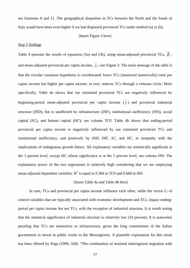
see footnotes 8 and 11. The geographical disparities in TCs between the North and the South of

Italy would have been even higher if we had displayed provincial TCs under method (a) or (b).

[Insert Figure 3 here]

Step 2 findings

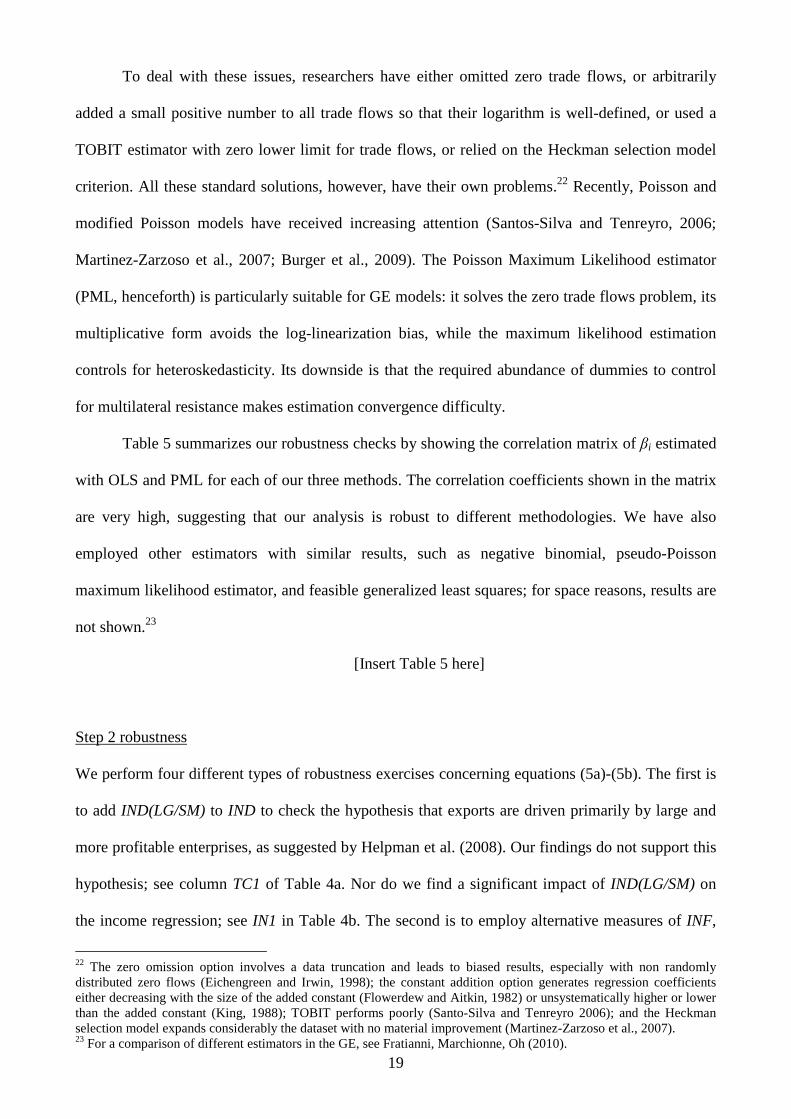
Table 4 presents the results of equations (5a) and (5b), using mean-adjusted provincial TCs, iβ ,

and mean-adjusted provincial per capita income, iy ; see Figure 3. The main message of the table is

that the circular causation hypothesis is corroborated: lower TCs (measured numerically) raise per

capita income but higher per capita income, in turn, reduces TCs through a virtuous circle. More

specifically, Table 4a shows that our estimated provincial TCs are negatively influenced by

beginning-period mean-adjusted provincial per capita income (y ) and provincial industrial

structure (IND), but is unaffected by infrastructure (INF), institutional inefficiency (INS), social

capital (SC), and human capital (HC); see column TC0. Table 4b shows that ending-period

provincial per capita income is negatively influenced by our estimated provincial TCs and

institutional inefficiency, and positively by IND, INF, SC, and HC, in sympathy with the

implications of endogenous growth theory. All explanatory variables are statistically significant at

the 1 percent level, except HC whose significance is at the 5 percent level; see column IN0. The

explanatory power of the two regressions is relatively high considering that we are employing

mean-adjusted dependent variables: R2 is equal to 0.384 in TC0 and 0.668 in IN0.

[Insert Table 4a and Table 4b here]

In sum, TCs and provincial per capita income influence each other, while the vector Ci of

control variables that are typically associated with economic development and TCs, impact ending-

period per capita income but not TCs, with the exception of industrial structure. It is worth noting

that the statistical significance of industrial structure is relatively low (10 percent). It is somewhat

puzzling that TCs are insensitive to infrastructure, given the long commitment of the Italian

government to invest in public works in the Mezzogiorno. A plausible explanation for this result

has been offered by Puga (1999, 328): “The combination of minimal interregional migration with

18

wage setting at the national sectoral level may help understand why infrastructure improvements

have failed to help the Italian Mezzogiorno catch with the North of the country...” With

interregional labor immobility and real wage differences, industrial spreading would occur with

firms relocating from high-wage-agglomerated (and congested) areas to low-wage-unagglomerated

areas. A common national wage rate, as it is true in Italy, could undo this mechanism.

VI. ROBUSTNESS

Step 1 robustness

Consider high-TC provinces that trade only with close countries. For those provinces bilateral trade

with long-distance countries would be counted as zero trade flows. Hence, there is a potential that

zero trade flows may bias upward the algebraic estimate of the distance elasticity. Under these

circumstances, a log-linear GE specification and OLS estimation may be inappropriate for three

reasons (Burger et al., 2009). The first has to do with the way zero trade flows are treated.20

Bilateral trade, at some level of disaggregation, is frequently zero or missing (Frankel, 1997;

Haveman and Hummels, 2004).21 Since these zeros do not occur randomly (Rauch, 1999), their

omission could bias the estimates of trade determinants (Linders and De Groot, 2006). The second

is the bias created by the logarithmic transformation: the concavity of the log function, under OLS,

imparts a downward bias because of the Jensen’s inequality (Haworth and Vincent, 1979). The third

is the failure of the homoskedasticity assumption. With non-negative exports, the variance of

exports conditional on exogenous variables declines as the conditional mean of exports approaches

the lower zero limit (Santo-Silva and Tenreyro, 2006). Trade data are potentially heteroskedastic,

whereas the log-normal model assumes homoskedasticity. In these cases, OLS estimations are

inconsistent and inefficient.

20 The assumption of log-normality in the random component implies the double-logarithmic specification that predicts positive trade flows. In contrast, the multiplicative GE can predict zero values. 21 Zeros can occur either because some country pairs do not trade, or rounding errors, or observations are mistakenly recorded as zero. Santos-Silva and Tenreyro (2006) reckon that measurement errors may pose a more serious problem than the log-linear transformation bias.

19

To deal with these issues, researchers have either omitted zero trade flows, or arbitrarily

added a small positive number to all trade flows so that their logarithm is well-defined, or used a

TOBIT estimator with zero lower limit for trade flows, or relied on the Heckman selection model

criterion. All these standard solutions, however, have their own problems.22 Recently, Poisson and

modified Poisson models have received increasing attention (Santos-Silva and Tenreyro, 2006;

Martinez-Zarzoso et al., 2007; Burger et al., 2009). The Poisson Maximum Likelihood estimator

(PML, henceforth) is particularly suitable for GE models: it solves the zero trade flows problem, its

multiplicative form avoids the log-linearization bias, while the maximum likelihood estimation

controls for heteroskedasticity. Its downside is that the required abundance of dummies to control

for multilateral resistance makes estimation convergence difficulty.

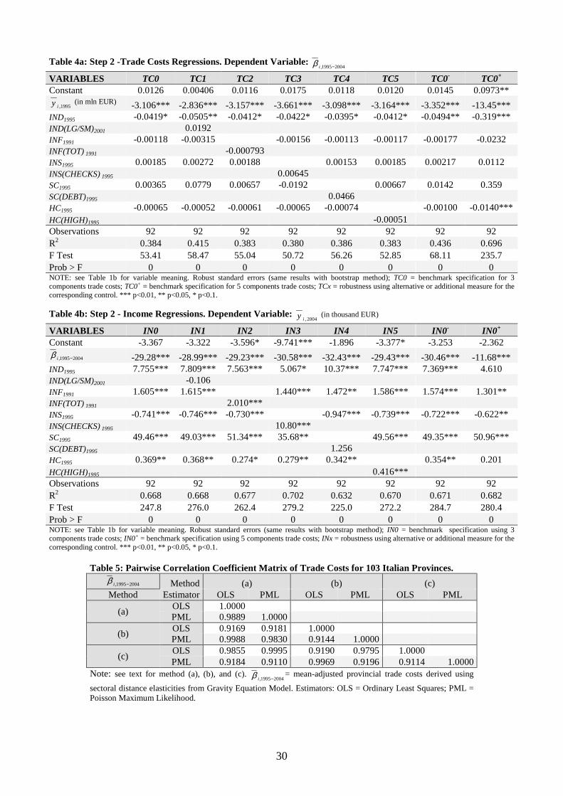
Table 5 summarizes our robustness checks by showing the correlation matrix of βi estimated

with OLS and PML for each of our three methods. The correlation coefficients shown in the matrix

are very high, suggesting that our analysis is robust to different methodologies. We have also

employed other estimators with similar results, such as negative binomial, pseudo-Poisson

maximum likelihood estimator, and feasible generalized least squares; for space reasons, results are

not shown.23

[Insert Table 5 here]

Step 2 robustness

We perform four different types of robustness exercises concerning equations (5a)-(5b). The first is

to add IND(LG/SM) to IND to check the hypothesis that exports are driven primarily by large and

more profitable enterprises, as suggested by Helpman et al. (2008). Our findings do not support this

hypothesis; see column TC1 of Table 4a. Nor do we find a significant impact of IND(LG/SM) on

the income regression; see IN1 in Table 4b. The second is to employ alternative measures of INF,

22 The zero omission option involves a data truncation and leads to biased results, especially with non randomly distributed zero flows (Eichengreen and Irwin, 1998); the constant addition option generates regression coefficients either decreasing with the size of the added constant (Flowerdew and Aitkin, 1982) or unsystematically higher or lower than the added constant (King, 1988); TOBIT performs poorly (Santo-Silva and Tenreyro 2006); and the Heckman selection model expands considerably the dataset with no material improvement (Martinez-Zarzoso et al., 2007). 23 For a comparison of different estimators in the GE, see Fratianni, Marchionne, Oh (2010).

20

INS, SC, and HC. The only significant changes in the income regression are: SC(DEBT) is not

statistically significant, whereas SC is; and HC becomes statistically less significant in the presence

of the INF and INS alternatives. No significant changes, on the other hand, take place in the trade

cost regressions. Overall, the coefficients are fairly stable and the main thrust of the message

remains. The third is to employ two alternative definitions of provincial TCs to our three-

component benchmark: a narrower one that excludes MONEY (because of its strong correlation

with RTA), and an expansive one that adds RTA and InterRTA (full specification of TCs). With the

narrower definition results are virtually the same for both regressions; see TC0- and IN0- of Table

4a-4b. With the expansive definition, IND and HC rise in statistical significance in the TC

regression (see TC0+ in Table 4a), whereas become insignificant in the income regression (see IN0+

in Table 4b). The implication is that under the expansive definition of TC, IND and HC affect

income indirectly through TCs. Our conclusion is that the instability of the RTA and InterRTA

coefficients in Table 3 argues for the benchmark TC specification. The final exercise relates to the

use of estimated parameters as regressors, that is the retrieval of the betas from step 1 to step 2. We

follow Saxonhouse (1976) and use a bootstrap procedure –with 100, 1,000 and 10,000 replications–

to estimate the standard errors of the parameter estimates. The results do not change with respect to

robust standard errors.

In sum, our robustness exercise confirms the main findings of the previous section.

VII. CONCLUSIONS

The key result of the paper is that regional economic development and trade costs in Italy

are related to each other through a circular causation pattern: lower TCs raise per capita income, but

higher per capita income, in turn, reduces TCs through a virtuous circle. Our approach consists of

two steps. In the first step, we estimate, with a gravity model, sectoral distance elasticities from 103

Italian provinces exporting 21 export categories to 188 countries under the restriction that these

elasticities are common to all provinces; these sectoral elasticities are then weighed by the

provincial export mix. Provincial TCs are the sum of several separate elasticities, of which only

21

one is a distance elasticity. By design, this approach ignores the potentially positive effects on TCs

emanating from the interaction of industrial sectors and location generated, among other things, by

agglomeration externalities. By so doing, our test works against our hypothesis. The spatial

distribution of provincial TCs appears to be consistent with the main implications of agglomeration

theory: with few exceptions, provinces in the “First Italy” (North-West) and “Third Italy” (North-

East and parts of the Center) face lower TCs than provinces in the developing South. To our

knowledge, this is the first paper that applies the gravity equation to trading pairs whose bilateral

distances differ by extremely small measure.

In the second step, we test the bi-directional causality between TCs and provincial per

capita income, our proxy of economic development, drawing from the insights of the New

Economic Geography. In addition to the interaction between trade costs and provincial per capita

income, we find that control variables that are typically associated with economic development

impact provincial per capita income but not TCs. We explain this finding, in part, with the

institutional practice in Italy to bargain for a nation-wide sectoral wage rate, a practice that tends to

counteract the positive effects of government investment programs in the poorer regions of the

country and reduces firms’ incentives to relocate from richer agglomerated to poorer non-

agglomerated areas.

One obvious policy implication of our paper is that government should promote reductions

of TCs through efficiency-increasing reforms that would benefit disproportionately the backward

regions of the country. The other policy implication, greatly opposed by trade unions, is to

encourage wage bargaining that would set wages at the regional rather than at the national level.

References

Anderson, J.E., 1979. A theoretical foundation for the gravity equation. American Economic Review, 69:106-16.

Anderson, J.E., van Wincoop, E., 2003. Gravity with gravitas: a solution to the border puzzle. American Economic Review, 93(1):170-192.

Anderson, J.E., van Wincoop, E.,2004. Trade costs. Journal of Economic Literature, 42(3):691-751.

22

Bagnasco, A., 1977. Tre Italie: la problematica territoriale dello sviluppo italiano. Bologna: Il Mulino.

Baier, S.L., Bergstrand, J.H., 2009. Bonus vetus OLS: A simple method for approximating international trade-cost effects using the gravity equation. Journal of International Economics, 77(1):77-85.

Baldwin, R., Taglioni, D., 2006. Gravity for Dummies and Dummies for Gravity Equations. NBER Working Paper 12516, http://www.nber.org/papers/w12516.

Becattini, G., 1990. The Marshallian industrial district as a socio-economic notion. In F. Pyke, G. Becattini and W. Sengenberger (eds.) Industrial districts and inter-firm co-operation in Italy, Geneva, International Institute for Labour Studies, 52-74.

Becattini, G., 2007. Il calabrone Italia. Bologna: Il Mulino.

Behrens, K., Lamorgese, A.R., Ottaviano, G.I.P., Tabuchi, T. 2007. Changes in transport and non-transport costs: Local vs global impacts in a spatial network. Regional Science and Urban Economics, 37:625–648.

Bergstrand, J.H., 1985. The gravity equation in international trade: some microeconomic foundations and empirical evidence. The Review of Economics and Statistics, 67(3):474-481.

Bergstrand, J.H., 1989. The generalized gravity equation, monopolistic competition, and the factor-proportions theory in international trade. The Review of Economics and Statistics, 71(1):143-153.

Bosker, M., Garretsen, H., 2007. Trade Costs, Market Access and Economic Geography: Why the Empirical Specification of Trade Costs Matters, CESIFO WP N. 2071, August.

Bosker, M., Brakman S., Garretsen, H., Schram, M. 2007. Adding geography to the new economic geography, CESIFO WP N. 2038, June.

Breusch, T., Pagan, A. (1979) A simple test of heteroskedasticity and random coefficient variation. Econometrica, 47:1287-1294.

Burger M.J., van Oort F.G., Linders G.J.M., 2009. On the Specification of the Gravity Model of Trade: Zeros, Excell Zeros and Zero-Inflated Estimation. Spatial Economic Analysis (forthcoming)

Brusco, S., 1990. The idea of the industrial district: Its genesis. In F. Pyke, G. Becattini and W. Sengenberger (eds.) Industrial districts and inter-firm co-operation in Italy, Geneva, International Institute for Labour Studies, 10-19.

Carrère, C., 2006. Revisiting the effects of regional trade agreements on trade flows with proper specification of the gravity model. European Economic Review, 50:223-247.

Central Intelligence Agency. World Factbook, https://www.cia.gov/library/publications/the-world-factbook/.

Chen, N., 2004. Intra-national versus international trade in the European Union: why do national borders matter? Journal of International Economics, 63:93–118.

Chenery, H.B. 1962. Development policies for Southern Italy, The Quarterly Journal of Economics, 76(4): 515:547.

Cheng, I.H., Wall, H.J., 2003. Controlling for heterogeneity in gravity models of trade and integration. Federal Reserve Bank of St. Louis Working Paper 1999-010D.

Deardorff, A.V., 1998. Determinants of bilateral trade: Does gravity work in a neoclassical world? In J. A. Frankel (ed.). The Regionalization of the World Economy. Chicago: University of Chicago Press.

Egger, P., 2000. A note on the proper econometric specification of the gravity equation. Economics Letters 66:25-31.

Eichengreen, B., Irwin, D.A., 1998. The role of history in bilateral trade flows, in (ed.). The Regionalization of the World Economy (Ed.) J.A. Frankel, University of Chicago Press, Chicago, 33-57.

European Commission. http://ec.europa.eu/economy_finance/euro/index_en.htm.

Faini, R., Galli, G., Gennari, P., Rossi, F. 1997. An empirical puzzle: Falling migration and growing unemployment differentials among Italian regions, European Economic Review, 41: 571-579.

Feenstra, R., 2003. Advanced international trade. Princeton, N.J.: Princeton University Press.

23

Fingleton, B. and P. McCann, 2007, Sinking the Iceberg? On the Treatment of Transport Costs in New Economic Geography, in B. Fingleton (ed.), New Directions in Economic Geography, Edward Elgar, pp. 168-204.

Flowerdew, R., Aitkin, M., 1982. A method of fitting the gravity model based on the Poisson distribution. Journal of Regional Science, 22:191-202.

Frankel, J.A., 1997. Regional trading blocs in the world trading system. Washington, DC: Institute for International Economics.

Frankel, J., Rose, A.K., 2002. An estimate of the effect of common currencies on trade and income. Quarterly Journal of Economics, 117:437-466.

Fratianni, M., Kang, H., 2006. Heterogeneous distance-elasticities in trade gravity models. Economics Letters, 90(1):68-71.

Fratianni, M., Marchionne, F., 2008. Heterogeneity In Trade Costs. Economics Bulletin, 6(48):1-14.

Fratianni, M., Marchionne, F., Oh, C.H. 2010. Commentary on the Gravity Equation in International Business, The Multinational Business Review, forthcoming.

Fratianni, M., Marchionne, F., 2011 (forthcoming). The limits to integration. In M.N. Jovanovic (ed.). International Handbook of Economic Integration. Elgar.

Fratianni, M., Oh, C.H. (2009). Expanding RTAs, trade flows, and the multinational enterprise. Journal of International Business Studies 40:1206-1227 doi:10.1057/jibs.2009.8

Gould, D., 1994. “Immigrant links to the home country: Empirical implications for U.S. bilateral trade flows. Review of Economics and Statistics, 69:301-316.

Guiso, L., Sapienza, P., Zingales, L., 2004. The Role of Social Capital in Financial Development. American Economic Review, 94(3):526-556.

Hausman, J.A., 1978. Specification tests in econometrics. Econometrica, 46(6):1251-1271.

Haveman, J., Hummels, D., 2004. Alternative hypotheses and the volume of trade: the gravity equation and the extent of specialization. Canadian Journal of Economics, 37(1):199-218.

Haworth, J.M., Vincent, P.J., 1979. The stochastic disturbance specification and its implications for log-linear regression. Environment and Planning A, 11:781-90.

Head, K., Mayer, T., 2004. The Empirics of Agglomeration and Trade. In Handbook of Regional and Urban Economics, Elsevier, 4(59):2609-69.

Head, K., Ries, J., 1998. Immigration and trade creation: Econometric evidence from Canada. Canadian Journal of Economics, 31:46-62.

Helliwell, J.F., 1998. How much do national borders matter? Washington, D.C.: The Brookings Institution.

Helliwell, J.F., 1999. Language and trade. In A. Breton(ed.) Exploring the economics of language, Ottawa, Department of Heritage, 26.

Helpman, E., Melitz, M., Rubinstein, Y., 2008. Estimating Trade Flows: Trading Partners and Trading Volumes. The Quarterly Journal of Economics, 123(2):441-487.

Hummels, D., 2007. Transportation costs and international trade in the second era of globalization. Journal of Economic Perspectives, 21(3):131-154.

Hummels, D., Ishii, J., Yi, K.M., 2001. The nature and growth of vertical specialization in world trade. Journal of International Economics, 54:75-96.

Hutchinson, W., 2002. Does ease of communication increase trade? Commonality of language and bilateral trade. Scottish Journal of Political Economy, 49:544-556.

ISTAT. I.Stat data warehouse, http://www.istat.it/dati/i_stat.html.

Istituto Tagliacarne. GeoWebStarter data warehouse, http://www.tagliacarne.it/gws/home.htm.

Kang, H., Fratianni, M., 2006. International trade, OECD membership, and religion. Open Economies Review, 17 (4-5):493-508.

24

King, G., 1988. Statistical models for political science event counts: bias in conventional procedures and evidence for the exponential Poisson regression model. American Journal of Political Science, 32:838-63.

Krugman, P., 1991. Increasing returns and economic geography. Journal of Political Economy, 99(3):483-499.

La Porta, R., Lopez-de-Silanes, F., Shleifer, A., Vishn, R., 2000. Investor protection and corporate governance. Journal of Financial Economics, 58:3-27.

Linders, G.J., De Groot, H.L.F., 2006. Estimation of the gravity equation in the presence of zero flows. Tinbergen Institute Discussion Paper, No.06-072/3, available at SSRN: http://ssrn.com/abstract=924160

Lucas, R.E., 1988. On the Mechanism of Economic Development. Journal of Monetary Economics, 22:3-42.

Lutz, V., 1962. Italy. A study in economic development. Oxford: Oxford University Press.

Markusen, A., 1996. Sticky places in slippery spaces: A typology of industrial districts. Economic Geography, 72(3):293-313.

Martin, P., Ottaviano, G.I.P., 2001. Growth and agglomeration. International Economic Review, 42(4):947-968.

Martinez-Zarzoso, I., Nowak-Lehmann, F.D., Vollmer, S., 2007. The Log of Gravity Revisited, available at SSRN: http://ssrn.com/abstract=999908.

McCallum, J., (1995) National borders matter: Canada–US regional trade patterns. American Economic Review, 85(3):615–623.

Mocetti, S. Porello, C. 2010. La mobilità del lavoro in Italia: nuove evidenze sulle dinamiche migratorie, Questioni di Economia e Finanza, Occasional Papers n. 61, Banca d’Italia, Roma.

Obstfeld, M., Rogoff, K., 2000. The six major puzzles in international macroeconomics: Is there a common cause? In B. Bernanke and K. Rogoff (eds.). NBER Macroeconomics Annual 2000, 339-390. Cambridge, MA: MIT Press.

Oh, C.H., 2006. Technical appendix on the regional economic integration database. In M. Fratianni (ed.) Regional Economic Integration. Amsterdam, Elsevier JAI.

Putnam, R., 1993. Making Democracy Work: Civic Tradition in Modern Italy. Princeton University Press. Princeton.

Putnam, R., Helliwell, J.F., 1995. Social Capital and Economic Growth in Italy. Eastern Economic Journal, 21:295-307.

Puga, D. 1999. The rise and fall of regional inequalities, European Economic Review, 43: 303-334.

Rauch, J.E., 1999. Networks versus markets in international trade. Journal of International Economics, 48:7–35.

Rauch, J.E., Trindade, V., 2001. Ethnic Chinese networks in international trade. Review of Economics and Statistics, 84:116-130.

Rose, A.K., 2000. One money, one market: the effect of currency unions on trade. Economic Policy, 30:7-46.

Rose, A.K., van Wincoop, E., 2001. National money as a barrier to trade: The real case for monetary union. American Economic Review, 91(2):386-390.

Santos-Silva, J.M.C., Tenreyro, S., 2006. The Log of Gravity. Review of Economics and Statistics, 88(4):641-658.

Saxonhouse, G.R., 1976. Estimated Parameters as Dependent Variables. American Economic Review, 66(1):178-183.

Venables, A.J., 1996. Equilibrium locations of vertically linked industries. International Economic Review, 37:341-59.

World Bank. World Development Indicators, World DataBank, http://databank.worldbank.org/ddp/home.do.

25

Table 1a: Descriptive Statistics of STEP 1 (millions of US dollars for Exports, Yi and Yj)

Panel A (N=103) Mean Median Stand.Dev. Min Max

Yi 11,315.7 6,967.2 15,809.2 1,284.0 154,822.0

ADJACENCY 0.155 0 0.362 0 1

Panel B (N=188) Mean Median Stand.Dev. Min Max

Yj 168,332.7 8,089.5 812,480.3 40.8 11,711,833.7

RTA 0.071 0 0.257 0 1

Inter-RTA 0.280 0 0.449 0 1

MONEY 0.032 0 0.176 0 1

ADJACENCY 0.022 0 0.147 0 1

Panel C (N=972,754) Mean Median Stand.Dev. Min Max

Exports 2.6 0.1 18.1 0.9 1,531.7

Yi 16,434.0 9,198.2 22,235.2 1,284.0 154,821.9

Yj 417,360.6 60,817.2 1,320,683.7 40.8 11,711,833.7

Distance 4,451 2,641 3,962 69 18,932

RTA 0.183 0 0.387 0 1

Inter-RTA 0.203 0 0.402 0 1

MONEY 0.089 0 0.285 0 1

ADJACENCY 0.003 0 0.057 0 1 NOTE: Panel A: statistics on provinces from ISTAT (i=103, j=1, k=1, t=10); Panel B: statistics on countries from World Development Indicator (i=1, j=188, k=1, t=10); Panel C: statistics on province-country-sector from ISTAT (i=103, j=188, k=21, t=10).

Table 1b: Descriptive Statistics of STEP 2 (Euro for iy )

Panel D (N=103) Mean Median Stand.Dev. Min Max

1995,iy 13,982 14,588 3,639 6,983 22,367

2004,iy 20,003 20,871 4,561 12,288 30,629

IND1995 0.334 0.320 0.181 0.080 0.879

IND(LG/SM)2001 0.401 0.329 0.293 0.010 1.640 INF1991 1.071 0.917 0.674 0.310 5.468 INF(TOT) 1991 1.014 0.885 0.598 0.293 5.083 INS1995 3.764 3.487 1.409 1.441 8.324 INS(CHECKS) 1995 0.478 0.480 0.160 0.091 0.880 SC1995 0.028 0.023 0.022 0.000 0.105 SC(DEBT)1995 0.029 0.024 0.031 0.000 0.157 HC1995 1.356 0.204 2.031 0.000 8.944 HC(HIGH)1995 1.244 0.180 1.882 0.000 8.354 NOTE: Income: y = provincial per-capita added value in euro (ISTAT). Industrial Structure: IND = industrial added value on total added value (ISTAT); IND(LG/SM) = added value of large on small-medium size firms (ISTAT). Infrastructure: INF = economic infrastructure composite index (TAGLIACARNE); INF(TOT) = total infrastructure composite index (TAGLIACARNE). Institutional Efficiency:

INS = years taken to complete a first-degree trial by provincial courts (Guiso, Sapienza, and Zingales, 2004);

INS(CHECKS) = frequency of residents who have used checks in the year (Guiso, Sapienza, and Zingales, 2004).

Social Capital: SC = number of blood bags per million inhabitants (Guiso, Sapienza, and Zingales, 2004);

SC(DEBT) = frequency of residents who have received loans from fiends and family (Guiso, Sapienza, and Zingales, 2004).

Human Capital: HC = first and second level degree for million inhabitants (TAGLIACARNE); HC(HIGH) = second level degree for million inhabitants (TAGLIACARNE).

26

Figure 1: Export distribution

0.0

25.0

5.0

75.1

.125

.15

Den

sity

0 5 10 15 20Ln(Xijkt)

Density Function of Ln(Xijkt)

Note: 972,754 observations. I=103, J=188, K=21, T=10.

Table 2: Value of cells in the trade matrix

Sector tji

tji

TotalCell

FullCell

,,

,,

Agriculture, Hunting, Forestry 0.31505371

Fish, Fishing Products 0.07920884

Coal, Lignite, Peat, Crude Petroleum, Natural Gas, Uranium, Thorium 0.03672795

Metal Ores, Other Mining, Quarrying Products 0.15978620

Food Products, Beverages, Tobacco 0.39478414

Textiles, Textile Products 0.41405701

Leather, Leather Products 0.30810783

Wood, Products of Wood, Cork (Except Furniture), Articles of Straw, Plaiting Materials 0.27897129

Pulp, Paper, Paper Products, Recorded Media, Printing Services 0.29880706

Coke, Refined Petroleum Products, Nuclear Fuel 0.09446395

Chemicals, Chemical Products, Man-Made Fibres 0.39609068

Rubber, Plastic Products 0.37533051

Other Non Metallic Mineral Products 0.37696757

Basic Metals, Fabricated Metal Products 0.42533051

Machinery and Equipment N.E.C. 0.51390725

Electrical and Optical Equipment 0.42727742

Transport Equipment 0.35043379

Other Manufactured Goods N.E.C. 0.39884321

Electrical Energy, Gas, Steam, Water 0.00343937

Real Estate, Renting, Business Services 0.08559182

Other Community, Social and Personal Services 0.06893720

27

Figure 2: Maps of 103 Italian Provinces: IND, INF, INS, SC, HC, and UN (Colors by quintiles).

NOTE: Sources are ISTAT, TAGLIACARNE, and Guiso, Sapienza, and Zingales (2004).

28

Table 3: Step 1 – OLS – Provincial distance interacting with sectors. 1995-2004 (N=972,754)

COEFFICIENT Method

(a) (b) (c) □

Year\Province\Country Dummies Yes\Yes\Yes Yes\No\No Yes\Yes\Yes Constant -7.632*** -17.53*** 1.256 ln(Y i) 0.503*** 0.903*** 0.247*** ln(Y j) 0.656*** 0.536*** 0.513*** ADJACENCY 0.669*** 1.505*** 0.745*** RTA -1.507*** -0.0557 -1.518*** inter-RTA -0.461*** 0.123*** -0.0826 MONEY 0.0971*** 0.0820*** 0.0790***

d*Agriculture, Hunting, Forestry -1.417*** -0.802*** -0.968***

d*Fish, Fishing Products -1.809*** -1.203*** -1.153***

d*Coal, Lignite, Peat, Crude Petroleum, Natural Gas, Uranium, Thorium -2.019*** -1.430*** -1.104***

d*Metal Ores, Other Mining, Quarrying Products -1.589*** -0.979*** -1.090***

d*Food Products, Beverages, Tobacco -1.243*** -0.621*** -0.858***

d*Textiles, Textile Products -1.232*** -0.604*** -0.816***

d*Leather, Leather Products -1.326*** -0.700*** -0.880***

d*Wood, Products of Wood, Cork (Except Furniture), Articles of Straw, Plaiting Materials -1.520*** -0.901*** -1.052***

d*Pulp. Paper, Paper Products, Recorded Media, Printing Services -1.406*** -0.780*** -0.954***

d*Coke, Refined Petroleum Products, Nuclear Fuel -1.596*** -0.998*** -0.951***

d*Chemicals, Chemical Products, Man-Made Fibres -1.203*** -0.579*** -0.823***

d*Rubber, Plastic Products -1.294*** -0.667*** -0.896***

d*Other Non Metallic Mineral Products -1.296*** -0.671*** -0.899***

d*Basic Metals, Fabricated Metal Products -1.221*** -0.593*** -0.829***

d*Machinery and Equipment N.E.C. -1.094*** -0.467*** -0.725***

d*Electrical and Optical Equipment -1.238*** -0.608*** -0.832***

d*Transport Equipment -1.284*** -0.658*** -0.858***

d*Other Manufactured Goods N.E.C. -1.270*** -0.641*** -0.866***

d*Electrical Energy, Gas, Steam, Water -1.829*** -1.258*** -1.115***

d*Real Estate, Renting, Business Services -1.859*** -1.254*** -1.286***

d*Other Community, Social and Personal Services -1.780*** -1.174*** -1.222***

Observations 972,754 972,754 625,734

Number of pairs 16,629 14,322

R2 0.438 0.352 0.431 F-test 336.5 49,406 162,374 Prob>F 0 0 0

LR-All2χ (Likelihood Ratio test statistic on province, country and time FE) 134,088.40 1,255.70 6,540.43

DoF LR-All (Degree of Freedom of Likelihood Ratio on province, country and time FE) 297 9 297

Prob LR-All >2χ (P-value of Likelihood Ratio test on province, country and time FE) 0 0 0

BPLM Test (Breusch-Pagan Lagrange Multiplier test statistics for RE) 1,793,847.00 187,342.50 DoF BPLM (Degree of Freedom of Breusch-Pagan Lagrange Multiplier test for RE) 1 1

Prob BPLM >2χ (P-value of Breusch-Pagan Lagrange Multiplier test for RE) 0 0

NOTE: See text for (a), (b), (c) methods. RE = random effects; FE = fixed effects. □ Exports over $30,000 for computational reasons. Cluster correction on pairs and robust standard errors: *** p<0.01, ** p<0.05, * p<0.1.

29

Figure 3: Maps of 103 Italian Provinces: per-capita GDP of 1995, trade costs over 1995-2004, and per-capita GDP of 2004.

Note: See text for methods (c). Green colors in the left and right maps represent mean-adjusted provincial per-capita GDP respectively for 1995 and 2004; ranges in the legend are common between these maps. Red colors in the middle map represents mean-adjusted provincial trade costs derived from 21 sectoral distance elasticities of Gravity Equation Model (Beta). In all maps, first and last ranges in the legend are larger than other ranges because they include extreme value.

30

Table 4a: Step 2 -Trade Costs Regressions. Dependent Variable: 20041995, −iβ

VARIABLES TC0 TC1 TC2 TC3 TC4 TC5 TC0- TC0+ Constant 0.0126 0.00406 0.0116 0.0175 0.0118 0.0120 0.0145 0.0973**

1995,iy (in mln EUR) -3.106*** -2.836*** -3.157*** -3.661*** -3.098*** -3.164*** -3.352*** -13.45*** IND1995 -0.0419* -0.0505** -0.0412* -0.0422* -0.0395* -0.0412* -0.0494** -0.319*** IND(LG/SM)2001 0.0192 INF1991 -0.00118 -0.00315 -0.00156 -0.00113 -0.00117 -0.00177 -0.0232 INF(TOT) 1991 -0.000793 INS1995 0.00185 0.00272 0.00188 0.00153 0.00185 0.00217 0.0112 INS(CHECKS) 1995 0.00645 SC1995 0.00365 0.0779 0.00657 -0.0192 0.00667 0.0142 0.359 SC(DEBT)1995 0.0466 HC1995 -0.00065 -0.00052 -0.00061 -0.00065 -0.00074 -0.00100 -0.0140*** HC(HIGH)1995 -0.00051 Observations 92 92 92 92 92 92 92 92 R2 0.384 0.415 0.383 0.380 0.386 0.383 0.436 0.696 F Test 53.41 58.47 55.04 50.72 56.26 52.85 68.11 235.7 Prob > F 0 0 0 0 0 0 0 0 NOTE: see Table 1b for variable meaning. Robust standard errors (same results with bootstrap method); TC0 = benchmark specification for 3 components trade costs; TC0+ = benchmark specification for 5 components trade costs; TCx = robustness using alternative or additional measure for the corresponding control. *** p<0.01, ** p<0.05, * p<0.1.

Table 4b: Step 2 - Income Regressions. Dependent Variable: 2004,iy (in thousand EUR)

VARIABLES IN0 IN1 IN2 IN3 IN4 IN5 IN0- IN0+ Constant -3.367 -3.322 -3.596* -9.741*** -1.896 -3.377* -3.253 -2.362

20041995, −iβ -29.28*** -28.99*** -29.23*** -30.58*** -32.43*** -29.43*** -30.46*** -11.68*** IND1995 7.755*** 7.809*** 7.563*** 5.067* 10.37*** 7.747*** 7.369*** 4.610 IND(LG/SM)2001 -0.106 INF1991 1.605*** 1.615*** 1.440*** 1.472** 1.586*** 1.574*** 1.301** INF(TOT) 1991 2.010*** INS1995 -0.741*** -0.746*** -0.730*** -0.947*** -0.739*** -0.722*** -0.622** INS(CHECKS) 1995 10.80*** SC1995 49.46*** 49.03*** 51.34*** 35.68** 49.56*** 49.35*** 50.96*** SC(DEBT)1995 1.256 HC1995 0.369** 0.368** 0.274* 0.279** 0.342** 0.354** 0.201 HC(HIGH)1995 0.416*** Observations 92 92 92 92 92 92 92 92 R2 0.668 0.668 0.677 0.702 0.632 0.670 0.671 0.682 F Test 247.8 276.0 262.4 279.2 225.0 272.2 284.7 280.4 Prob > F 0 0 0 0 0 0 0 0 NOTE: see Table 1b for variable meaning. Robust standard errors (same results with bootstrap method); IN0 = benchmark specification using 3 components trade costs; IN0+ = benchmark specification using 5 components trade costs; INx = robustness using alternative or additional measure for the corresponding control. *** p<0.01, ** p<0.05, * p<0.1.

Table 5: Pairwise Correlation Coefficient Matrix of Trade Costs for 103 Italian Provinces.

20041995, −iβ Method (a) (b) (c) Method Estimator OLS PML OLS PML OLS PML

(a) OLS 1.0000 PML 0.9889 1.0000

(b) OLS 0.9169 0.9181 1.0000 PML 0.9988 0.9830 0.9144 1.0000

(c) OLS 0.9855 0.9995 0.9190 0.9795 1.0000 PML 0.9184 0.9110 0.9969 0.9196 0.9114 1.0000

Note: see text for method (a), (b), and (c). 20041995, −iβ = mean-adjusted provincial trade costs derived using

sectoral distance elasticities from Gravity Equation Model. Estimators: OLS = Ordinary Least Squares; PML = Poisson Maximum Likelihood.