Export Intensity and Input Trade Costs: Evidence from ChineseFirms�

Miaojie Yuy Wei Tianz

China Center for Economic Research Guanghua School of ManagementPeking University Peking University

Preliminary and Comments Welcome

July 15, 2012

Abstract

How do reductions in input trade costs a¤ect �rm�s sales decision between domestic and foreign

markets? Aside from tari¤s cut in ordinary imports over time, a large extent of �rms to engage in

duty-free processing trade also leads to a decline in input trade cost. Accordingly, the imported input

tari¤s reduction/exemption introduces �rms to access more imported intermediate inputs and then

export a larger proportion of �nal products since, compared to goods for domestic sales, exporting

goods use better-quality imported intermediate inputs. By using Chinese �rm-level production data

and transaction-level trade data during 2000-2006 to construct �rm-speci�c input trade costs, we

�nd rich evidence that a reduction in input trade cost leads to an increase in export intensity (i.e.,

exports over total sales). Such results are robust to di¤erent empirical speci�cation and econometric

methods.

JEL: F1, F2

Keywords: Export Intensity, Input Trade Cost, Imported Intermediate Inputs, Processing

Trade

�We thank Robert Feenstra, Chang-Tai Hsieh, Brad Jensen, Samuel Kortum, Justin Lin, James Tybout, Yang Yaoand seminar and conference participants from the 14th NBER-CCER conference, the 2nd China Trade Research Group(CTRG) conference, the 3rd IEFS (China) conference, Zhejiang University, Nankai University, and Shanghai School ofForeign Trade for their helpful comments and constructive suggestions. However, all errors are ours.

yChina Center for Economic Research (CCER), National School of Development, Peking University, Beijing 100871,China. Phone: 86-10-6275-3109, Fax: 86-10-6275-1474, E-mail: mjyu@ccer.pku.edu.cn.

zDepartment of Applied Economics, Guanghua School of Management, Peking University. Email:wei.tian08@gmail.com.

1 Introduction

Trade liberalization is one of the most important topics in international trade. It is of particular

interests for both academia and policy makers to understand �rm�s decision in choosing markets when

a country experiences gradual trade liberalization. Traditionally, import tari¤s reduction on �nal

goods is regarded as generating tougher import competition, which in turn force domestic �rms to

adjust their export intensity�the proportion of exports over total sales. Today, research interests on

trade liberalization have been switched from output tari¤ reductions to input tari¤ reductions (see, for

example, Amit and Konings 2007; Topalova and Khandelwal, 2011). However, there are still relatively

little research on �rm�s response to adjust its export intensity upon facing tari¤s reductions in import

tari¤s. The present paper tries to �ll in this gap.

This paper investigates the e¤ects of changing input trade costs on �rm�s export intensity using a

very rich matched Chinese �rm-level production data and transaction-level trade data. A novel element

of the paper is that input trade costs are measured at and tailored to the �rm-level, which allow us to

exactly measure the input trade costs faced by a �rm. Firms face declining input trade costs over the

sample period 2000-2006 from two sources. First, gradual tari¤s reduction in ordinary imports occurs

over time after China acceded to the WTO in 2001. More interestingly, a large extent of Chinese �rms

self-select to engage in processing trade in which they could enjoy the free import duties. Thus, the

declining input trade costs introduce �rms to access more imported intermediate inputs, which in turn

transfer to higher export intensity for two reasons.

Firstly, by de�nition, more processing imports imply more processing exports. When �rms self-

select to engage in a larger extent to processing trade, a larger proportion of their �nal products

would sell abroad. Secondly and more interestingly, evidence from the Chinese transaction-level trade

data reported in the paper suggests that imported intermediate goods used for producing exporting

�nal goods have better quality than those used for producing non-exporting �nal goods (i.e., goods

sold in the domestic market). With a declining input trade cost, �rms would use more better-quality

intermediate inputs. As a consequence, �rms could generate more pro�ts from foreign market than from

1

domestic market hence secure a larger export intensity. To elaborate this point, a simple Melitz-type

model is deliever in the paper to shed light on the mechanism.

To accurately estimate the impact of input trade cost on export intensity, we also control for the

other two types of trade liberalization: import tari¤s on �nal goods and external tari¤s set by Chinese

trading partners. As mentioned above, output tari¤s reduction in �nal goods also generates tougher

import competition, which could in turn change �rm�s export intensity. Meanwhile, during the sample

period over 2000-2006, many Chinese �rms export a variety of products to many countries. Chinese

exporters also enjoyed large tari¤ reductions in their export destinations. With reductions in foreign

trade costs, �rms are able to access to larger foreign markets which could possibly result in a larger

export intensity. We hence construct the �rm-level external tari¤s to measure the weighted tari¤s

across trading countries and across products over years. However, although the most ideal way is

to obtain a corresponding �rm-level import output tari¤s, data on each product�s domestic sales are

unavailable, we hence only control for industry-level output import tari¤s in the estimates.

As perhaps the most important feature of international trade in China, processing trade refers to

the process by which a domestic �rm initially obtains raw materials or intermediate inputs abroad,

and after local processing, exports their value-added �nal goods. Processing trade in China enjoys the

privilege of tari¤ exemptions. To fully capture the impact of processing trade on �rm�s export intensity,

we adopt three di¤erent measures to examine the role of processing trade. We start using a processing

dummy to distinguish processing �rms from non-processing (i.e., ordinary) �rms. However, �rm�s

decision to engage in processing is endogenous. Less productive �rms or foreign-invested �rms in China

are more likely to engage in processing trade (Yu, 2011). We hence estimate the probability of �rms

engaging in processing trade, and adopt the Heckman (1979) two-step approach to explore the e¤ect

of �rm�s predicted processing probability on export intensity. Finally, �rm�s input trade cost would be

much di¤erent among �rms with di¤erent extent to processing. We hence use a continuous variable�the

extent to processing which is measured by processing imports over total imports�to highlight the role

of processing trade on �rm�s export intensity.

We then decompose and identify the sources of variation in �rm-level input trade costs. Firms

may engage in processing trade or may not. Input tari¤ reduction would have a signi�cant e¤ect on

2

non-processing �rm�s behavior like export intensity, but should not be so for pure-processing �rms that

100% engage in processing trade since processing trade is already de-facto duty-free. Yet, perhaps the

most interesting case is of hybrid �rms which engage in both processing and ordinary trade. Thus, the

variation of hybrid �rm�s input trade costs could come from two di¤erent components: input tari¤s

reduction in ordinary imports and/or the proportion allocation between processing and ordinary import

components. Such information is carried to construct the �rm-speci�c input tari¤. Beyond this, we

also identify sources of variation in input trade costs by di¤erent types of �rms: pure ordinary, pure

processing, and hybrid �rms. Of course, some �rms could switch from processing to ordinary trade,

or vice versa. We hence also look at the e¤ect of input trade costs on �rm�s export intensity for such

switching �rms speci�cally.

But, in which ways does the reduction in input trade cost a¤ect �rm�s export intensity? Are

they through the extensive margin, or intensive margin, or both? To check this out, we separate

exporters to three types: new exporters, exiters, and continuing exporters. In particular, we �nd that

the declining input trade cost not only increases the probability of �rm�s being new exporters (i.e.,

extensive margin) but also leads to a higher export intensity (i.e., intensive margin). However, the

impact of either extensive margin or intensive margin is insigni�cant for exiting �rms. By contrast, the

impact of intensive margin is signi�cant for continuing exporters. A similar �nding are present when

we turn the interest to the extensive margin��rm�s export scopes.

The endogeneity of �rm-speci�c input trade costs is also carefully discussed and addressed. Three

di¤erent sources of endogeneity exist for the constructed �rm input tari¤s. As �rm�s export intensity

is de�ned as export over sales, the �rst endogeneity issue is the possible reverse causality of sales on

tari¤s. Firms with small amount of sales may blame their bad market situation to tougher import

competition due to trade liberation. Accordingly, they would lobby the government for protection. We

therefore adopt an instrumental variable (IV) approach to control for such a possible reverse causality.

The second endogeneity comes from the possible reserve causality of �rm�s exports on its imports.

Firm�s exports are highly correlated with its imports. The last endogeneity issue raises from the

measure of the input tari¤s itself. Suppose that a �rm faces a prohibitive tari¤ line for a product that

it wishes to import, such a tari¤ is not included in �rm�s input tari¤s due to its zero import. However,

3

the �rm indeed faces a high tari¤ (but not zero tari¤). To control for these two endogeneity issues,

we use �rm�s imports in the �rst year of the sample to construct a �xed weight for �rm-speci�c input

tari¤s following Topalova and Khandelwal (2011). After controlling for a variety of endogeneity issues,

we still �nd robust evidence that input tari¤ reduction leads to an increase in export intensity.

Finally, we also perform two important robustness checks. The �rst exercise is to consider the

relative importance of domestic intermediate inputs against imported intermediate inputs and carry

such di¤erence to construct an alternative measure of input tari¤s, which also suggests very similar

results as our previous estimates: The declining trade cost reduction leads to an increase in export

intensity.

Our last robustness check is to adopt the quantile estimates to examine the heterogenous impact

of input trade cost on �rm�s export intensity by di¤erent quantiles. We �rst look at their response at

the four quartiles and then examine them carefully in which quantiles are allowed to be measured at

a continuum version. Both types of quantile analysis yield similar results as the standard �xed-e¤ects

OLS estimates. They also help us understand the economic magnitude of the estimates: A one-point

decrease in �rm-speci�c input trade costs would lead to around a 5.2% increase in its export intensity.

This paper joins a growing literature on both counts. The �rst is on the topic of export intensity.

Previous studies have recognized that �rms only sell a small fraction of their output abroad. This

is documented by, among others, Bernard and Jensen (1995), Tybout (2001), Bernard et al. (2010),

Arkolakis and Muendler (2010), and Eaton et al. (2011). Most of such studies focus on interpreting why

export intensity is small. Speci�cally, Bernard et al. (2003) emphasized a key reason for large countries

like the United States is the existence of a relatively large domestic market. Brooks (2005) argued the

key reason for small countries like Columbia is due to the low quality of their export products. Asides

from these, Bonaccorsi (1992) found evidence that �rm�s export intensity is positively associated with

its size using Italian manufacturing industry-level data. Greenaway et al. (2004) investigated whether

spillovers a¤ect a �rm�s export propensity using British �rm-level data.

However, there are still very limited research for China though it has become the second largest

economy and largest exporter in the world. As documented in the later section, although China

shares a common phenomenon with other countries in the sense that Chinese �rms only export a small

4

proportion of their products, there still exist a sizable proportion of �rms that exports all of their

products. Such a pattern is known as the U-shape as also observed in Lu (2011).1 Therefore, it is

worthwhile to ask how the declining input trade costs a¤ect such Chinese �rms�export pattern, which

hence adds value to the related literature.

Another set of related literature is on input trade liberalization. Among many other papers, Amiti

and Konings (2007) found that �rm�s gain from the reduction of input tari¤s is at least twice as much as

those from cutting output tari¤s by using Indonesian �rm-level data. Topalova and Khandelwal (2011)

con�rm that such a gain di¤erence could be exaggerated to approximately ten times in magnitude in

several industries in India. Turning to the application to China, Yu (2011) found that the declining

output tari¤s still have a larger impact on �rm productivity than the reduction in input tari¤s due, in

large part, to the fact that processing trade in China is duty-free. However, to our limited knowledge,

rare studies, if any, consider the impact of input trade cost on �rm�s export intensity despite both

being tropical topics in the �eld.

The remainder of the paper is organized as follows. Section 2 introduces a theoretical model to

guide our empirical analysis. Section 3 describes data used in the present paper. Section 4 introduces

our measures for key variables and empirical speci�cations. Section 5 presents the estimation results

and sensitivity analysis. Finally, Section 6 concludes.

2 Theoretical Framework

The aim of this section is to deliver a theoretical framework to provide some guidelines for the subse-

quently empirical analysis, though we have no ambition to develop a general theoretical model. For

this purpose, we extend the Melitz-type(2003) model by allowing two types of inputs (i.e., labor and

intermediate inputs) and introducing imported intermediate inputs to the model a là Halpern et al.

(2011).

To investigate the impact of input trade cost on �rm�s export intensity, consider an exporter with

productivity ' that serves in both domestic market and foreign market which has production functions

1Lu et al. (2010) also use Chinese �rm-level data to �nd that, among foreign a¢ liates, exporters are less productive

than non-exporters. Dai et al. (2012) points out the key reason for such a phonomenon is due to the prevalence of

processing trade in China.

5

as follows:

qr = 'L�M (1��)

r ;8r = d; x (1)

where qr;8r = d; x denotes domestic sales (qd) and foreign sales (qx), respectively. L is labor and M is

intermediate inputs. ' is �rm productivity. The intermediate input is assembled from a combination

of domestic and imported intermediate inputs. As suggested by Feng et al. (2012), �rms that use more

imported intermediate inputs are associated with more exports. One possible reason for this �nding

is that exporting goods use more imported intermediate inputs than those goods sold in the domestic

market. Accordingly, the intermediate input production function is assumed to take the following form:

Mr =

�(ArMF )

��1� +M

��1�

H

� ���1

;8r = d; x (2)

whereMr;8r = d; x is the intermediate inputs for �nal goods sold domestically (Md) and abroad (Mx).

MF is imported intermediate inputs and MH is domestic intermediate inputs. � > 1 is the elasticity

of substitution between imported intermediate inputs and domestic intermediate inputs. The larger

the elasticity �, the less the di¤erence between imported and domestic intermediate inputs. Ad and

Ax represents the e¢ ciency of combining imported inputs to produce �nal products that sell at home

and abroad, respectively.

Compared to goods sold in domestic markets, the imported intermediate goods used for export

�nal goods are presumed to have better quality (Ax > Ad). This is possibly because exporting �rms or

plants have better foreign network. They are able to access imported intermediate inputs with better

quality. As shown in the following empirical parts, such a conjecture is highly supported by Chinese

�rm data.

By normalizing price of the domestic intermediate inputs as one, the aggregated price of intermedi-

ate input for domestic sales (Sd) and foreign sales (Sx) can be obtained by solving the cost-minimization

problem in (2):

Sr =�Sh + (Sf=Ar)

1��� 11��

=�1 +B��1r

� 11��

;8r = d; x

where Sh (Sf ) is the price of domestic (imported) intermediate inputs. The second equality is obtained

by normalizing the price of domestic intermediate inputs as a unity and using the notation that

Br = Ar=Sf ;8r = d; x. Note that Sr < 1 since Br > 0 and � > 1. Clearly, the better quality

6

of the imported inputs, the higher price of the aggregated price index for intermediate inputs. As

suggested by Halpern et al.(2011), the intuition is that combining imported intermediate inputs with

domestic intermediate inputs is more productive than "the sum of the parts" in line with the idea of

Hirschman (1958). Accordingly, the combined intermediate inputs have higher prices than the domestic

intermediate inputs.

Meanwhile, �rm�s input trade cost (�) provides a wedge between domestic import price Sf and world

price p�. That is, Sf = p�(1+�). For simplicity, we assume that the input trade costs have no any terms-

of-trade e¤ect like the case in a small open economy. Accordingly, we have dBr=d� < 0;8r = d; x. The

intuition is straightforward: a decrease in input trade costs transfers to a decrease in price of imported

intermediate inputs which in turn leads to an increase in imported intermediate inputs.

Accordingly, the cost functions associated with production functions for domestic sales (Cd) and

foreign sales (Cx) are:

Cr = (f + qr=')w��1 +B��1r

� 1��1��

;8r = d; x (3)

where f is the �xed costs of production and w is wages as in Melitz (2003).

In a monopolistic-competition environment, the equilibrium pricing rule implies that �rm�s marginal

revenue equals marginal cost. Given that the representative consumer has a utility of constant elasticity

� as in Melitz (2003), the domestic price (pd) faced by the �rm with productivity ' is:

pd(') =w��1 +B��1d

� 1��1��

�';

where � = (��1)=�. Meanwhile, the price faced by the �rm with productivity ' in the foreign market

is:

px(') =�w�

�1 +B��1x

� 1��1��

�';

where � is the tari¤s set by foreign trading countries. With such pricing rules, the �rm�s domestic

revenue is:

rd(') = Eh(w���'P )��1(1 +B��1d )

(1��)(��1)��1 ; (4)

where Eh is home�s aggregate expenditure where P is the aggregate price index.2 Similarly, the �rm�s

2As in Melitz (2003), the aggregate price index is P =�R10p(')1��M�(')d'

� 1��1where M is the mass of �rms with

distribution �(') in an industry.

7

export sales is:

rx(') = n�1��Ef (w

���'P )��1(1 +B��1x )(1��)(��1)

��1 : (5)

where n denotes the number of trading countries whereas � is additional marginal cost of serving foreign

market like import tari¤s. For simplicity, foreign countries are assumed to be symmetric. Accordingly,

foreign import tari¤s � and foreign country�s aggregate expenditure Ef are identical for all countries.

Firm�s pro�t at the domestic market (�d) and foreign market (�x) can be written as:

�d(') =Eh�(w���'P )��1(1 +B��1d )

(1��)(��1)��1 � f; (6)

and

�x(') =n�1��

�Ef (w

���'P )��1(1 +B��1x )(1��)(��1)

��1 � fx; (7)

where fx is the exporting �xed costs. Firm�s pro�t is the combination of domestic pro�t and foreign

pro�t: �(') = �d(') + �x('). Clearly, we have:

Proposition 1 A decrease in �rm�s input trade cost leads to an increase in �rm�s total pro�t (d�d� <

0).

Proof. See Appendix A1.

Thus far, �rm�s export intensity (�) can be easily obtained from (4) and (5). To be more straight-

forward, we consider the inverse function of �rm�s export intensity as follows:

1

�� rx(') + rd(')

rx(')

= 1 +Eh

n�1��Ef

1 +B��1d

1 +B��1x

! (1��)(��1)��1

:

Hence, we can obtain the following testable prediction:

Proposition 2 A decrease in �rm�s input trade cost leads to an increase in exporting �rm�s export

intensity ( d�d� < 0) if imported intermediate inputs used for export have high quality than those used for

domestic sales (Ax > Ad).

Proof. See Appendix A2.

8

The economic intuition is straightforward. If imported intermediate inputs used for export are of

better quality, the exported �nal goods can generate more pro�t since their price is relatively higher

than �nal goods for domestic sales. Trade liberalization secures �rms to access more intermediate

inputs. Thus, the more the better imported intermediate inputs are used for exports, the higher the

�rm pro�t, and hence the larger the �rm export intensity. Put another way, with tari¤ reductions,

export sales increase faster than domestic sales since exporting goods have higher prices since they use

higher-quality inputs.

We now turn to the empirical section to see whether such a theoretical prediction is supported by

Chinese �rm-level data.

3 Data

To investigate the impact of trade liberalization on �rm�s export intensity, this paper uses the following

three disaggregated large panel data sets: tari¤s data, �rm-level production data, and product-level

trade data.

Tari¤ data can be accessed directly from the WTO.3 China�s tari¤ data are available at HS six-digit

level over years 2000�2006, which are less disaggregated than HS 8-digit transaction-level trade data.4

We hence �rst aggreate transaction-level trade data to HS 6-digit level in concord with tari¤s data.

We use average Ad Valorem duty to measure trade liberalization given that our main interest is to

estimate the e¤ect of trade liberalization on export intensity.

3.1 Firm-Level Production Data

The sample used in this paper comes from a rich �rm-level panel dataset which covers around 230,000

manufacturing �rms per year over 2000-2006. The data are collected and maintained by China�s

National Bureau of Statistics in an annual survey of manufacturing enterprises. It contains entire in-

formation of three accounting sheets (i.e., Balance Sheet, Loss & Bene�t Sheet, and Cash Flow Sheet).

On average, the annual entire value of industrial production covered in such a data set accounts for

3 source of the data: http://tari¤data.wto.org/ReportersAndProducts.aspx.4China did not report its tari¤s data to the WTO during 1998-2000. However, data from 1997 are available. As

reported in Customs Import & Export Tari¤ of the P.R. C. (various years), China did not experience dramatic tari¤

reductions in 1998-2000, hence the 1997 tari¤s are used as serve proxy for those of 2000.

9

around 95% of China�s total industrial production by year. Indeed, aggregated data on the indus-

trial sector in the annual China�s Statistical Yearbook by the Natural Bureau of Statistics (NBS) are

compiled from this dataset. The dataset includes more than 100 �nancial variables listed in the main

accounting sheets of all these �rms. Brie�y, it covers two types of manufacturing �rms: (1) all SOEs;

(2) non-SOEs whose annual sales are more than �ve million RMB. As shown in Column (3) of Table

A1, the number of �rms that ever occurred in the dataset is 615,951 in total.

However, the raw production data set is still quite noisy since it still includes many unquali�ed

�rms with poor accounting systems.5 Following Cai-Liu (2009), Feenstra-Li-Yu (2011), we delete

observations according to the basic rules of Generally Accepted Accounting Principles if any of the

following are true: (1) liquid assets are higher than total assets; (2) total �xed assets are larger than

total assets; (3) the net value of �xed assets is larger than total assets; (4) number of employees is less

than eight peole as suggested by Brandt et al.(2011); (4) the �rm�s identi�cation number is missing;

or (5) �rm�s established time is invalid (e.g., the opening month is later than December or earlier than

January). Accordingly, the total number of �rms covered in the data set is reduced to 438,165, around

1/3 of �rms are dropped from the sample after such a �lter process. As shown in Column (4) of Table

A1, the attrition ratio is even higher in the initial years of the dataset: around 1/2 of �rms are dropped

in 2000.

3.2 Product-Level Trade Data

The disaggregated transaction-level monthly trade data during 2000-2006 are obtained from China�s

General Administration of Customs. As shown in Column (1) of Table A1, the annual number of

observations increase from around 10 million in 2000 to around 16 million in 2006, ending with a huge

number of observations, 118,333,831, in total for seven years. Column (2) of Table A1 exhibits that

there are 286,819 �rms that ever engage in international trade during this period.

For each transaction, the data set compiles three types of information: (1) basic trade information

which includes value (measured at US current dollar), trade status (export or import), quantity, trade

unit, and value per unit. (2) Trade mode and pattern such as destination country for exports, original

5For example, some family-based �rms, which usually have no formal accounting system in place, reports their pro-

duction information based on a unit of one RMB, whereas the o¢ cial requirement is a unit of 1000 RMB.

10

country for imports, routing countries (i.e., whether the product is shipped through an intermediate

country/regime), customs regime (e.g., processing trade or ordinary trade), transport mode (i.e., by

sea, by truck, by air, or by post), and customs port (i.e., where the product departs or arrives). (3)

Firm-level transaction information. In particular, it includes seven variables such as �rm�s name,

identi�cation number set by the customs, city where the �rm is located, telephone, zip code, name

of the manager/CEO, and even ownership type of �rm (e.g., foreign a¢ liate, private, or state-own-

enterprises).

We then match transaction-level trade data, �rm-level production data, and tari¤s data together.

Since trade data and production data has no common identication numbers, the matching is of par-

ticular challenge. The detailed method and technique is decribed carefully in the Appendix. Brie�y,

the matched data accounts for around 40% of exporters in terms of number of �rms and around 70%

of export value.

4 Measures and Empirics

4.1 Firm-Speci�c Input Tari¤s

A �rm could import many products in di¤erent amounts. Since its imported intermediate input could

vary arcoss industries, an aggregated industry-level tari¤ is insu¢ cient to capture �rm heterogeneity

within a sector. Therefore, it is essential to construct a �rm-speci�c variable of input trade costs.

A special feature of China�s import tari¤s is that processing imports in China are duty-free. More

interestingly, di¤erent types of processing imports have di¤erent tari¤ treatments (Yu, 2011). In

the reality, China has around 20 types of processing trade. But two of them are most important:

Processing with assembly and processing with inputs (Feenstra and Hanson, 2005). They have two

main key di¤erences in such two types:

Firstly, processing with assembly refer to the process that �rms passively receive materials from

their foreign clients. In contrast, processing with inputs refer to the process that �rms can make their

own decision to import foreign intermediates or raw materials. Secondly, processing with assembly is

100% duty-free. By contrast, processing with inputs have to pay the input duty upon importation,

and get a full-fund duty rebate when the processed �nal goods are exported. As a result, such �rms

11

still bear the opportunity cost of paying the import duty.

Therefore, we construct a �rm-speci�c input tari¤ index (FITit) as follows:

FITit =Xk2O

mkitP

k2M mkit

�kt + 0:05Xk2I

mkitP

k2M mkit

�kt ; (8)

where mkit is �rm i�s import value on product k in year t and, as before, �kt is the ad valorem tari¤

of product k in year t. O is the set of �rm�s ordinary imports, I is the set of all processing imports

other than processing with assembly, and M is the set of �rm�s total imports. That is, O [ I[ A = M

where A is the set of processing with assembly and by de�nition, is 100% duty free. Thus, this set is

not included in Eq. (8). Note that the �rst term in Eq. (8) measures the input tari¤s from ordinary

imports, whereas the second term measures those from processing with inputs in which �rms have to

pay the import duties on imported materials from abroad but can get the full-amount duty rebate once

the �nal value-added products export. Thus, �rms engaged in processing with inputs have stronger

demands on cash �ow and have to bear extra risk-free interest�Otherwise �rms could alternatively use

the funds paid to cover their duty to invest at a risk-free rate. We hence follow Hsieh-Klenow (2009)

to set the real interest rate to 0.05.6

4.2 Firm-Speci�c External Tari¤s

To measure the tari¤ reductions in a �rm�s export destinations, we construct an index of �rm-speci�c

external tari¤s (FETit ) as follows:

FETit =Xk

"(XkitP

kXkit

)Xc

(XciktP

cXcikt

)� ckt

#; (9)

where � ckt is product k�s ad valorem tari¤ imposed by export destination country c at year t. A �rm

may export multiple types of products to multiple countries. The ratio in the second parentheses in

Eq. (9), Xcikt=

PcX

cikt, measures the export ratio of product k produced by �rm i but consumed in

country c, yielding a weighted external tari¤ across Chinese �rms�export destinations. Similarly, the

�rst parenthesis in Eq. (9), Xkit=PkX

kit, measures the proportion of product k�s exports over �rm i�s

total exports.6Usually the processing activities could be done within a year (see Yu and Tian, 2012). Accordingly, �rms only bear

a one-year real risk-free interest rate. However, changing the number of China�s real interest rate such as 1% or 3% does

not a¤ect our estimates at all.

12

As a control variable, the output import tari¤s are measured at industrial level. Lower output

import tari¤s induce tougher import competition. To measure the impact of import competition, it is

ideal to have information on domestic sales at product-level so that the output tari¤s can be tailored

to the �rm level. A possible proxy is to presume that the proportion of domestic sales to total sales is

the same as that of exports to total sales for each product (Yu, 2011). However, such an assumption

may be inappropriate given that our key interest of this project is to investigate the share of �rm�s

export over sales. We hence measure the output tari¤s at the industry level.

4.3 Estimation Framework

To investigate the e¤ect of input tari¤ reductions on �rm export intensity, we then consider an empirical

framework as follows:

Exp_intijt = �0 + �1FITit + �2FETit + �3FETit � PEit + �4OTjt (10)

+�5OTjt � PEit + �4PEit + �Xit + �i + �t + �it; (11)

where Exp_intijt measures �rm�s export intensity for �rm i in industry j in year t, as discussed before.

FITit and FETit denote �rm-speci�c weighted input tari¤ and external tari¤ in year t respectively.

PEit is a processing indicator which equals one if �rm i engages in processing activity in year t,

and zero otherwise. OTjt denotes industry-level tari¤s for industry j in year t. Xit denotes other �rm

characteristics such as type of ownership (i.e., state-owned-enterprises or multinational �rms), �rm size

(i.e., log employment), and �rm productivity. Finally, the error term is divided into three components:

(1) �rm-speci�c �xed e¤ects �i to control for time-invariant factors such as a �rm�s location; (2) year-

speci�c �xed e¤ects �t to control for �rm-invariant factors such as China�s accession to the WTO in

2001 and Chinese RMB appreciation after 2005; (3) an idiosyncratic e¤ect �it with normal distribution

�it s N(0; �2i ) to control for other unspeci�ed factors.

5 Empirical Results

5.1 Benchmark Results

As described above, the attrition rate of the merged data set is high, though it is a suitable represen-

tative of the full-sample �rm data. Therefore, it is reasonable to ask whether such a high attrition

13

rate a¤ects estimation results. Hence our estimations begin from a comparison between the full-sample

data set and merged data set. Column (1) of Table 2 reports the estimates using full-sample �rm-level

data. Without merging with the transaction-level trade data, the �rm-level data have no information

on products, so it is impossible to measure input tari¤s at the �rm level. We hence abstract away

the �rm input tari¤s but only keep output industry tari¤s. Hence, the estimate in Column (1) with

a full-sample of 725,993 observations concentrates on the impact on �rm export intensity of output

tari¤s, which is measured at the HS 2-digit industry-level. Clearly, industrial output tari¤s are pos-

itively associated with �rm�s export intensity. Column (2) includes more control variables like SOEs

and foreign indicators and yields the similar results in both magnitudes and signs. Column (3) drops

the two extreme values of export intensity (i.e., zero and one) and, again, obtain similar results.

The rest of Table 2 runs regressions by using the merged data set. For a close comparison, Columns

(4)-(6) of Table 2 perform the exact identical estimates as their counterparts in Columns (1)-(3). Once

again, the coe¢ cients of industry tari¤s are all positive signi�cant, indicating the use of matched data

is a suitable representative of the full-sample data set.

Of all the speci�cations in Table 2, �rm�s ownership matters for �rm export intensity as well.

The statistically signi�cant and positive coe¢ cients of the foreign indicator suggest that multinational

a¢ liates have higher export intensity. Similarly, after controlling for �rm-speci�c and year-speci�c �xed

e¤ects, the negative and signi�cant signs of SOEs indicator suggest that SOEs sell a larger proportion

of their products at home.

[Insert Table 2 Here]

Before adopting the matched samples to perform the estimations, it is worthwhile to check whether

the distribution of �rm�s export intensity in the full sample is similar to that in the matched sample.

If not, then our estimation results would be a suspect. As seen from Figure 1, �rm�s export intensity

in the matched-sample shows a U-shape in the LHS of Figure 1B, which is very similar to that in the

full-sample in the LHS of Figure 1A. Of course, around 72% of �rms do not export in the full-sample

production �rm-level dataset whereas only 17% of �rms do not export in the matched data set given

that the matched data, by construction, only cover trading �rms (i.e., either export or import, or

both). Therefore, the density for the extreme values of �rm�s export intensity (i.e., zero and one)

14

would be di¤erent. However, their non-parametric kernel density after dropping the two-side extreme

values are very similar, as shown in the RHS of Figure 1A and 1B. Therefore, the matched data set

is a good representative of the full-sample data set. Finally, as suggested by Ahn et al. (2011), the

carry-along trading importers and exporters (i.e., intermediaries) would have di¤erent production and

sales behavior. For instance, indirect trading exporters would sell their 100% of their products abroad.

We therefore drop both indirect trading exporters and importers from our sample in all estimates.

[Insert Figure 1 Here]

To investigate the impact of �rm-speci�c input tari¤s reduction on export intensity, we start from

plotting �rm�s export intensity against �rm-speci�c input tari¤s, which are aggregated in industry

level over years. Figure 2 clearly suggests a negative correlation between the average �rm-speci�c

export intensity and input tari¤s. Of course, such a negative correlation could be just driven by other

unspeci�ed factors. In addition to the output import tari¤s reductions, the tari¤s reduction in China�s

trading partners may also a¤ect Chinese �rm�s export intensity. Thus, controlling for tari¤ reduction

in China�s export destinations is also worthwhile in obtaining the precise estimate of the e¤ect of

import tari¤ reductions on a �rm�s export intensity. We then control for industrial output tari¤s and

�rm-speci�c external tari¤s as well as �rm�s type of ownership (i.e., SOEs and foreign �rms) and trade

regime (i.e., processing and ordinary �rms) in all estimates in Table 3.

To understand the overall impact of input tari¤ reduction on export intensity, estimate in Column

(1) starts from abstracting away the interaction role of various tari¤s reduction and �rm�s processing

status. After controlling for �rm-speci�c �xed e¤ects and year-speci�c �xed e¤ects, estimates in Col-

umn (1) show that �rm�s input tari¤s reduction leads to larger proportion of exports to sales, though

the impact of industrial output tari¤s and �rm-speci�c external tari¤s on export intensity is insigni�-

cant. Adding the interaction terms between processing dummy and input tari¤s (external tari¤s, and

output tari¤s) does not change the estimation results in terms of signs or magnitudes.

One may concern that the large proportion of pure domestic �rms which have zero export may

a¤ects our estimation results given that around 17% of Chinese �rms have zero exports in our matched

data. A similar argument applies to a fairly large proportion of pure exporting �rms�12% exporters

export all of their products. Meanwhile, some Chinese �rms notably do not have their own production

15

activity, but only export goods collected from other domestic �rms or import goods from abroad and

then sell to other domestic companies (Ahn et al., 2011). Such �rms would result in a unit of export

intensity. We hence drop �rms which export intensity is zero in Column (4) and one in Column (5).

Column (6) goes further to drop observations if export intensity is either zero or one. Neither of such

speci�cations change our estimation results for the key variable: the coe¢ cient of �rm input tari¤ is

always negative and highly signi�cant at conventional statistical level.

[Insert Table 3 Here]

5.2 Discussion on the Impact Channels

It is interesting to ask why input tari¤s reduction can lead to higher export intensity. One possible

reason is that input tari¤s reduction generates more �rm pro�tability (i.e., �rm�s pro�t over sales) which

in turn introduces higher export intensity (export over sales). Given that higher �rm pro�tability is

positively associated with higher export intensity, the key interest is how reduction in input trade costs

generates more �rm pro�tability. This could come from two channels. The �rst one is from the change

of �rm markup. Input tari¤s reduction could have a cost-saving e¤ect for �rms and hence raise the

price-to-cost markup. Another possibility is that lower tari¤s make �rms access to more input varieties

which in turn foster more pro�t.

To check whether such conjectures are supported by data, Column (1) of Table 4 �rst includes �rm�s

markup, which is measured by �rm�s revenue over the di¤erence between revenue minus pro�t following

Keller and Yeaple (2009). It turns out the coe¢ cient of �rm�s markup is negative but insigni�cant.

However, when we include the interaction terms between �rm markup and the three tari¤ variables,

the variable of markup itself turns to be positively signi�cant. In addition, �rm-speci�c input tari¤ is

negative signi�cant whereas its interaction with �rm markup is positive signi�cant, indicating that �rm

markup is an important channel of input tari¤s on �rm�s export intensity. Meanwhile, the signi�cant

term of �rm input tari¤s suggests the existence of other channels.

In our sample, many Chinese �rms export multiple products, with the maximum even reaching

745 (see Table 1). We hence include a variable of �rm�s import scope in Column (3) which yields a

signi�cant and positive sign. Similarly, we add its interaction term with the three tari¤ variables. As

16

seen from Column (4), the coe¢ cient of input tari¤ is negative and signi�cant whereas its interaction

term with import scope is also negative and signi�cant, suggesting that access to more import varieties

is an important channel for �rms to realize higher export intensity from input tari¤s reduction. The

negative sign of the interaction term between �rm input tari¤s and �rm import scope also suggests that

�rms with more import varieties can increase more export intensity from their input tari¤s reduction.

[Insert Table 4 Here]

In fact, such a theoretical conjecture is well supported by Chinese trade data. By using unit-

value of imports as a proxy of quality as suggested by Hallak (2006), Column (1) of Table 1 shows

that the intermediate inputs used for processing imports have better quality than those for ordinary

imports. By de�nition, processing intermediate imports are used for export only. In contrast, ordinary

intermediate imports could be used to produce goods for either exports or domestic sales. Thus, the

fact that the unit-price of intermediate processing imports is higher than that of intermeidate ordinary

imports suggests that imported intermediate goods for exports have better quality than imported

intermediate goods for domestic sales. Such an observation is even true when the intermediate inputs

are broken-down to sub-catogories including parts & components and semi-�nished goods according

to the classi�cation of broader economic categories (BEC) as shown in Columns (2)-(3) of Table 1.

[Insert Table 8 Here]

5.3 Sources of the Input Trade Costs Reduction

Figure 2B demonstrates that the average �rm input tari¤s across industries exhibited a declining trend

over the period 2000-2006 which witness China�s trade liberalization in the period. It is worthwhile to

ask where are the sources of the �rm-speci�c input tari¤s. The �rst answer that come to our minds is

due to the tari¤s reduction of products that �rms import. In the measure of �rm-speci�c input tari¤s

(8), if �kt decreases, �rm input tari¤s FITit would decrease even other components are unchanged.7

Meanwhile, there still exist another source for input tari¤s reduction. When faced by some negative

7Of course, when tari¤ �kt decreases, the import weight mkit for the product k for �rm i could change as well. However,

change the weight to a �xed weight using the initial year in the period (mki;2000) or a �oating one-period lag weight (m

kit�1)

does not change our estimation results.

17

demand shocks, �rms may adjust their production structure between processing imports and ordinary

imports. Since processing activities has a lower threshold to entry, �rms may engage in more processing

activities when they are in a short position in the market (Yu, 2011). If �rms have more weights in

processing activities, they would be able to bear a lower �rm-speci�c input tari¤s. However, in the

reality such two sources are combined automatically. Therefore, it is worthwhile to decompose the two

sources and identify their e¤ects.

Table 5 therefore picks up such a task. In the estimate of Column (1), only pure ordinary �rms are

included in which �rm-speci�c input tari¤ only has its �rst component FITit =X

k2��mkitP

k2�mkit

�kt .

Similarly, Column (2) only covers pure processing �rms in which �rm-speci�c input tari¤ only has

its second component FITit = 0:05�X

k2��mkitP

k2�mkit�kt

�. Column (3) covers hybrid �rms that have

some ordinary imports and some processing imports. However, since the �rm-speci�c tari¤s (8) still

re�ects the changes in both processing share and tari¤s change, we �x the tari¤s by using the tari¤s

line for products in the initial years so that one can clearly observe the impact of changing process-

ing share on the export intensity. That is, the �rm-speci�c tari¤ in Column (3) is measured asXk2��

mkitP

k2�mkit�k2000 + 0:05

Xk2~�

mkitP

k2�mkit�k2000. It turns out that the coe¢ cients of �rm-speci�c in-

put tari¤s are negative and signi�cant in Columns (1)-(3), indicating that changes in both tari¤s and

processing share matters for �rms to realizing the increase in their export share.

We now go further to explore the transition probability for the trade regime switch. As shown in

Appendix Table A4, it is more likely for �rms to switch from pure processing �rms to hybrid �rms,

but less likely for �rms to switch from hybrid �rms to non-hybrid �rms or from ordinary �rms to

non-ordinary �rms. The reason is straightforward. Given that the threshold of processing trade is

low in China, pure ordinary �rms would entry to processing trade only when the market is tough. In

contrast, pure processing �rms would start to engage in ordinary trade if the market is soft. Columns

(4)-(6) hence preform the estimates for �rms that switch from ordinary to hybrid, from pure processing

to hybrid, and from hybrid to non-hybrid �rms, respectively. It turns out that only the e¤ect of input

tari¤ on export intensity for �rms that switch from ordinary to hybrid are negative and signi�cant.

[Insert Table 5 Here]

18

5.4 Estimates for Entry and Exit

As suggested by Blum et al. (2012), Chilean �rms would reduce their domestic sales when they enter

foreign markets. Meanwhile, for continuing exporters, Chilean �rms� foreign and domestic sales are

negatively correlated over time. Having explored the sources of the variation of input trade costs, we

now ask whether the impact of �rm�s input trade costs on export intensity is di¤erent across starter,

continuing �rms, and exiters. Column (1) of Table 6 includes only starters that include both exporters

and non-exporters whereas Column (2) includes new exporters only. Similarly, Columns (3) and (4)

includes all exiters and exiting exporters, respectively. Columns (5)-(6) covers continuing �rms and

continuing exporters, respectively. It turns out that the coe¢ cients of �rm-speci�c input tari¤s are

negative and signi�cant. Interestingly, the magnitudes for starters and exiters in Columns (1)-(4)

are more pronounced than those continuing �rms in Columns (5)-(6), suggesting that the e¤ect of

reduction in �rm input trade costs on export intensity are more important for starters and exiters.

[Insert Table 6 Here]

5.5 First-Di¤erence Estimates

Firm�s export intensity could be a¤ected by other factors that are unspeci�ed in the estimations above.

Although we have employed �rm-speci�c �xed-e¤ects and year-speci�c �xed-e¤ects to control for factors

that are only variant across �rms and over years, respectively. It is still possible to exist some other

omitted factors that change both across �rms and over years. For instance, China�s government is

allowed some exportable products to enjoy the previledge of "export value-added tax rebate". Such

value-added tax rebate ratio di¤ers across industries and over year8, though the detailed data are

not reported either in �rm-level data or transaction-level data. We hence perform the following �rst-

di¤erence estimate to control for such possible omitted variables as suggested by Tre�er (2004):

�Exp_intijt = �0 + �1�FITit + �2�FETit + �3�FETit � PEit + �4�OTjt (12)

+�5�OTjt � PEit + �4PEit + �Xit +$i + �t + �it; (13)

8Most commodities are mandatory to pay 13% or 17% value-added tax for their value-added in China. However, if

such commodities are exportable goods, �rms can get the value-added tax rebate when such products are exported. The

value-added tax rate is set as 5%, 9%, 11%, 13%, or 17% which is contigent on products.

19

where �yit is the �rst-di¤erence of the variable yit 2nExp_intijt; F ITit; FETit; OTjt

odenoting yit�

yit�1:We also include the �rm (year)-speci�c �xed e¤ects to control for the time-invariant (variant)

growth factors.

As shown in Column (1) of Table 7, the variable of �rst-di¤erence in �rm-input tari¤s is still

negative and signi�cant. To check whether such results are sensitive to the extreme values of the

variable of export intensity, we drop samples with zero export intensity in Column (2) and samples

with a unit of export intensity in Column (3). Finally, we even drop samples which export intensity is

zero or one. All of such speci�cations have a similar result: the reduction in �rm-speci�c input tari¤s

leads to an increasing export intensity.

[Insert Table 7 Here]

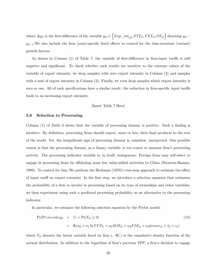
5.6 Selection to Processing

Column (1) of Table 3 shows that the variable of processing dummy is positive. Such a �nding is

intuitive. By de�nition, processing �rms should export, more or less, their �nal products to the rest

of the world. Yet, the insigni�cant sign of processing dummy is, somehow, unexpected. One possible

reason is that the processing dummy, as a binary variable, is too coarse to measure �rm�s processing

activity. The processing indicator variable is, in itself, endogenous. Foreign �rms may self-select to

engage in processing �rms by o¤shoring some low value-added activities to China (Feenstra-Hansen,

1999). To control for this, We perform the Heckman (1979)�s two-step approach to estimate the e¤ect

of input tari¤ on export extensity. In the �rst step, we introduce a selection equation that estimates

the probability of a �rm to involve in processing based on its type of ownerships and other variables,

we then experiment using such a predicted processing probability as an alternative to the processing

indicator.

In particular, we estimate the following selection equation by the Probit model:

Pr(Pr oces sin git = 1) = Pr(Vit � 0) (14)

= �(�0 + �1 lnTFPit + �2SOEit + �3FIEit + �2tenureit + �j + &t)

where Vit denotes the latent variable faced by �rm i. �(:) is the cumulative density function of the

normal distribution. In addition to the logarithm of �rm�s previous TFP, a �rm�s decision to engage

20

in processing trade is also a¤ected by other factors such as �rm�s productivity (measured by the Olley-

Pakes total factor productivity). The Heckman two-step approach requires a restriction variable that

is statistically signi�cant in the �rst-step but not in the second-step. The variable of �rm�s tenure

(tenureit) that measure �rm�s age is proposed to serve as such a variable. Finally, we also include the

HS 2-digit level industrial dummies �j and year dummies &t to control for other unspeci�ed factors.

Table 8 reports the estimation results for the selection equation (14) using the Probit model. We

see that foreign �rms are more likely to engage in processing trade. Similarly, �rms that established

earlier (i.e., larger tenure) are more likely to engage in processing trade. SOEs and low productive

�rms are less likely to become processing �rms, though their coe¢ cients are insigni�cant.

[Insert Table 8 Here]

Columns (1)-(2) of Table 9 then report the second-step estimation results by replacing the process-

ing indicator with predicted processing probability for Eq. (14). The predicted processing probability

produces a mean higher that of the processing indicator, as shown in the summary statistics of Table

1. We starts from Column (1) to include all observations but drop extreme values of export intensity in

Column (2). In both estimates, �rm�s tenure are found to be insigni�cant in the second-step estimates,

suggesting that �rm�s tenure is an appropriate restrictive variable. By contrast, the inverse Mills ratios,

which is de�ned as the probability density function over cumulative density function for the residual

that obtained in the linear estimation in the �rst-step, are included in the current second-step estimates

and found to be signi�cant. Once again, the coe¢ cients of �rm-speci�c input tari¤s are negative and

signi�cant. Meanwhile, the coe¢ cients of processing indicators now turn to be positive and signi�cant.

[Insert Table 9 Here]

In the reality, some �rms only engage a small proportion of its output in processing trade whereas

some other �rms engage in a large proportion. Ignoring such a di¤erence may not be able to capture the

production di¤erence across �rms. To overcome such an identi�cation challenge, we then take a step

forward to consider a continuous measure of the extent to which a �rm is engaged in processing trade

to replace the predicted processing probability. In particular, the extent of processing engagement

is measured through a �rm�s total processing imports over total imports in each year. We estimate

21

the e¤ect of �rm-speci�c input tari¤ on export intensity in Columns (3)-(4) of Table 9, by using the

variable of extent to processing to replace the processing probability. Once again, the coe¢ cients of

�rm-speci�c input tari¤s are negative and signi�cant, indicating that input tari¤ reduction leads to

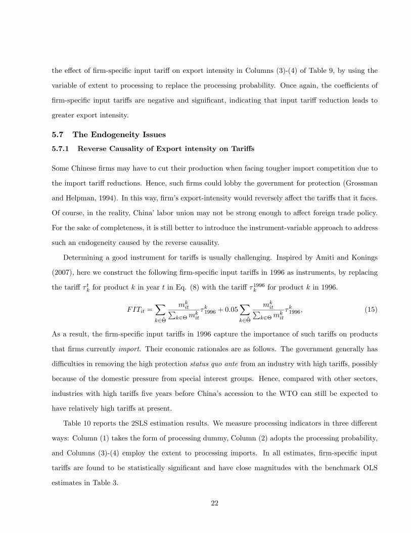
greater export intensity.

5.7 The Endogeneity Issues

5.7.1 Reverse Causality of Export intensity on Tari¤s

Some Chinese �rms may have to cut their production when facing tougher import competition due to

the import tari¤ reductions. Hence, such �rms could lobby the government for protection (Grossman

and Helpman, 1994). In this way, �rm�s export-intensity would reversely a¤ect the tari¤s that it faces.

Of course, in the reality, China�labor union may not be strong enough to a¤ect foreign trade policy.

For the sake of completeness, it is still better to introduce the instrument-variable approach to address

such an endogeneity caused by the reverse causality.

Determining a good instrument for tari¤s is usually challenging. Inspired by Amiti and Konings

(2007), here we construct the following �rm-speci�c input tari¤s in 1996 as instruments, by replacing

the tari¤ � tk for product k in year t in Eq. (8) with the tari¤ �1996k for product k in 1996.

FITit =Xk2��

mkitP

k2�mkit

�k1996 + 0:05Xk2~�

mkitP

k2�mkit

�k1996; (15)

As a result, the �rm-speci�c input tari¤s in 1996 capture the importance of such tari¤s on products

that �rms currently import. Their economic rationales are as follows. The government generally has

di¢ culties in removing the high protection status quo ante from an industry with high tari¤s, possibly

because of the domestic pressure from special interest groups. Hence, compared with other sectors,

industries with high tari¤s �ve years before China�s accession to the WTO can still be expected to

have relatively high tari¤s at present.

Table 10 reports the 2SLS estimation results. We measure processing indicators in three di¤erent

ways: Column (1) takes the form of processing dummy, Column (2) adopts the processing probability,

and Columns (3)-(4) employ the extent to processing imports. In all estimates, �rm-speci�c input

tari¤s are found to be statistically signi�cant and have close magnitudes with the benchmark OLS

estimates in Table 3.

22

A �nal remark is that the coe¢ cient of TFP is negative and signi�cant, indicating that high

productive Chinese �rms have lower export intensity. This �nding indeed is suggested by Lu (2011)

who documents that Chinese exporters have lower productivities than non-exporters. One possible

reason could be due to the processing trade (Dai, et al., 2012) who con�rm the �nding suggested by

Yu (2011) that less productive �rms are more likely to engage in processing trade. In any case, the

exploration of Chinese �rms�TFP is out of the scope of the current project, though it is an interesting

future work.

Several tests were performed to verify the quality of the instruments. First, we check whether such

an exclusive instruments are "relevant". That is, whether they are correlated with the endogenous

regressors (i.e., the current �rm�s input tari¤s). In our econometric model, the error term is assumed

to be heteroskedastic: �it s N(0; �2i ). Therefore, the usual Anderson (1984) canonical correlation

likelihood ratio test is invalid because it only works under the homoskedastic assumption of the error

term. Instead, we use the Kleibergen�Paap (2006) Wald statistic to check whether the excluded

instruments correlate with the endogenous regressors. As shown in Table 10, the null hypothesis that

the model is under-identi�ed is rejected at the 1% signi�cance level.

Second, we test whether or not the instruments are weakly correlated with the �rm�s current input

tari¤s. If so, then the estimates will perform poorly in the IV estimate. The Anderson-Rubin Wald

�2 tests provide strong evidence to reject the null hypothesis that the �rst stage is weakly identi�ed

at a highly signi�cant level.

Finally, the �rst-stage estimates reported in the lower module of Table 10 o¤er more supportive

evidence to justify such instruments. In particular, all the t-values of the instruments are signi�cant.

The excluded F�statistics in the �rst stage are also highly signi�cant. Thus, these statistical tests

provide su¢ cient evidence that the instrument performs well and, therefore, the speci�cation is well

justi�ed.

[Insert Table 10 Here]

23

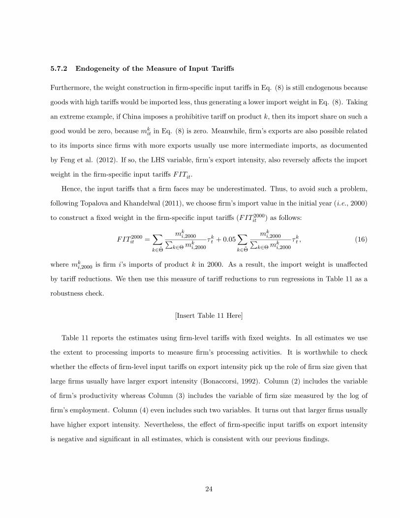
5.7.2 Endogeneity of the Measure of Input Tari¤s

Furthermore, the weight construction in �rm-speci�c input tari¤s in Eq. (8) is still endogenous because

goods with high tari¤s would be imported less, thus generating a lower import weight in Eq. (8). Taking

an extreme example, if China imposes a prohibitive tari¤ on product k, then its import share on such a

good would be zero, because mkit in Eq. (8) is zero. Meanwhile, �rm�s exports are also possible related

to its imports since �rms with more exports usually use more intermediate imports, as documented

by Feng et al. (2012). If so, the LHS variable, �rm�s export intensity, also reversely a¤ects the import

weight in the �rm-speci�c input tari¤s FITit.

Hence, the input tari¤s that a �rm faces may be underestimated. Thus, to avoid such a problem,

following Topalova and Khandelwal (2011), we choose �rm�s import value in the initial year (i.e., 2000)

to construct a �xed weight in the �rm-speci�c input tari¤s (FIT 2000it ) as follows:

FIT 2000it =Xk2��

mki;2000P

k2�mki;2000

�kt + 0:05Xk2~�

mki;2000P

k2�mki;2000

�kt ; (16)

where mki;2000 is �rm i�s imports of product k in 2000. As a result, the import weight is una¤ected

by tari¤ reductions. We then use this measure of tari¤ reductions to run regressions in Table 11 as a

robustness check.

[Insert Table 11 Here]

Table 11 reports the estimates using �rm-level tari¤s with �xed weights. In all estimates we use

the extent to processing imports to measure �rm�s processing activities. It is worthwhile to check

whether the e¤ects of �rm-level input tari¤s on export intensity pick up the role of �rm size given that

large �rms usually have larger export intensity (Bonaccorsi, 1992). Column (2) includes the variable

of �rm�s productivity whereas Column (3) includes the variable of �rm size measured by the log of

�rm�s employment. Column (4) even includes such two variables. It turns out that larger �rms usually

have higher export intensity. Nevertheless, the e¤ect of �rm-speci�c input tari¤s on export intensity

is negative and signi�cant in all estimates, which is consistent with our previous �ndings.

24

5.8 Additional Estimates with Alternative Measure of Input Tari¤s

Thus far, we have seen rich evidences that the input tari¤ reduction leads to an increase in �rm�s

export intensity. Our �nal work is to provide additional estimates with alternative measure of input

tari¤s as a robustness check.

The key variable, �rm-speci�c input tari¤ FITit have captured the importance of each product for

a �rm. However, in the reality, some �rms use more intermediate inputs whereas some other �rms may

use more domestic inputs. It is worthwhile to incorporate such information into the index. We hence

consider the following index

FITAltit =

Pk2�m

kit

Inputit

0@Xk2��

mkitP

k2�mkit

�kt + 0:05Xk2~�

mkitP

k2�mkit

�kt

1A ; (17)

where Inputit is �rm�s use of total intermediate inputs which include both imported inputs and domestic

inputs. Table 12 adopts such an alternative measure of input tari¤s to replace the FITit but still yields

very similar results for all estimates: the reduction in �rm�s input trade cost leads to an increase in

export intensity. The intuition is straightforward, the e¤ect of the �rst �rm (Pk2�m

kit)=Inputit shown

in (17) are indeed captured by the estimate coe¢ cients in all the previous tables.

[Insert Table 12 Here]

5.9 Further Quantile Estimates

A possible concern is whether or not the OLS estimates is appropriate for estimation given that

the sample of �rm�s export intensity exhibits a U-shape, which is far from the normal distribution

that requires for OLS estimates. However, this is not a problem since that the U-shape of �rm�s

export intensity across �rms is due, in large part, to the variation of �rm�s characteristics. Given that

we have already controlled for �rm-speci�c �xed-e¤ects and year-speci�c �xed e¤ects, such omitted

characteristics have been well controlled.

However, the U-shape of �rm�s export intensity also hints us that the response of input trade cost

to export intensity may not be identical across all �rms. The �xed-e¤ect OLS estimates so far only

focus on the mean level of the response of �rm input tari¤. The rich heterogeneity across all �rms are

hence abstracted away. To gain a better understanding the economic magnitude of the e¤ect of input

25

trade cost on �rm export intensity, the quantile estimates would be a plus to help us identify such

heterogenous magnitudes across �rms.

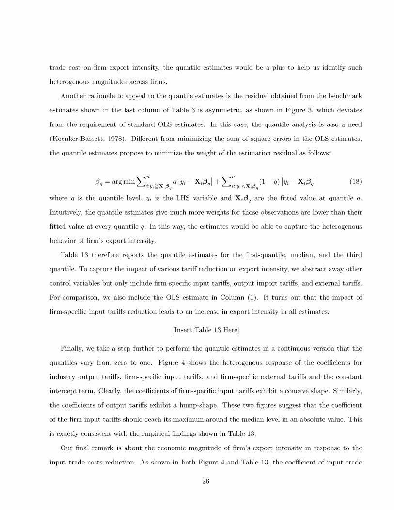
Another rationale to appeal to the quantile estimates is the residual obtained from the benchmark

estimates shown in the last column of Table 3 is asymmetric, as shown in Figure 3, which deviates

from the requirement of standard OLS estimates. In this case, the quantile analysis is also a need

(Koenker-Bassett, 1978). Di¤erent from minimizing the sum of square errors in the OLS estimates,

the quantile estimates propose to minimize the weight of the estimation residual as follows:

�q = argminXn

i:yi=Xi�qq��yi �Xi�q��+Xn

i::yi<Xi�q(1� q)

��yi �Xi�q�� (18)

where q is the quantile level, yi is the LHS variable and Xi�q are the �tted value at quantile q.

Intuitively, the quantile estimates give much more weights for those observations are lower than their

�tted value at every quantile q. In this way, the estimates would be able to capture the heterogenous

behavior of �rm�s export intensity.

Table 13 therefore reports the quantile estimates for the �rst-quantile, median, and the third

quantile. To capture the impact of various tari¤ reduction on export intensity, we abstract away other

control variables but only include �rm-speci�c input tari¤s, output import tari¤s, and external tari¤s.

For comparison, we also include the OLS estimate in Column (1). It turns out that the impact of

�rm-speci�c input tari¤s reduction leads to an increase in export intensity in all estimates.

[Insert Table 13 Here]

Finally, we take a step further to perform the quantile estimates in a continuous version that the

quantiles vary from zero to one. Figure 4 shows the heterogenous response of the coe¢ cients for

industry output tari¤s, �rm-speci�c input tari¤s, and �rm-speci�c external tari¤s and the constant

intercept term. Clearly, the coe¢ cients of �rm-speci�c input tari¤s exhibit a concave shape. Similarly,

the coe¢ cients of output tari¤s exhibit a hump-shape. These two �gures suggest that the coe¢ cient

of the �rm input tari¤s should reach its maximum around the median level in an absolute value. This

is exactly consistent with the empirical �ndings shown in Table 13.

Our �nal remark is about the economic magnitude of �rm�s export intensity in response to the

input trade costs reduction. As shown in both Figure 4 and Table 13, the coe¢ cient of input trade

26

cost reaches, in the absolute value, its maximum of 0.052 at the mean level but records a relatively

low number of 0.016 at the �rst-quarter level and of 0.035 at the third-quarter level. This suggests

that a one-percent declining in input trade costs leads to 5.2% increase in export intensity for �rms

around median level of export intensity, and 1.6 (3.5) % increase in export intensity for �rms around

�rst (third)-quarter level of export intensity. Given that the mean of input trade costs is 2.73% and

of export intensity is 48.8% as shown in Table 1, and 53% (58%) for �rms with �rst (third)-quarter

export intensity.

[Insert Figure 4 Here]

6 Concluding Remarks

The paper explores how reductions in tari¤s on imported inputs a¤ect �rms� export intensity by

exploiting the special tari¤ treatment a¤orded to the imported inputs by processing �rms as opposed

to non-processing �rms in China. As a popular trade pattern in a large number of developing countries,

including China, processing trade plays an important role in a variation of export intensity for �rms.

Since processing trade in China enjoys zero tari¤s on imported inputs, We �nd that a reduction in

input tari¤s leads to an increase in export intensity.

The present paper is one of the �rst to explore the role of processing trade on Chinese �rm�s export

share. The rich data set enables the determination of whether a �rm engages in processing trade and

the examination of the e¤ect of the �rms�extent of processing trade engagement on export intensity.

With such information, �rm-speci�c input tari¤s were also constructed, as one of the �rst attempts

in the literature, which, in turn, enriches the understanding of the economic e¤ect of the special tari¤

reform in processing trade.

27

References[1] Ahn, JaeBin, Amit Khandelwal, and Shang-jin Wei (2011), "The Role of Intermediaries in Facil-

itating Trade," Journal of International Economics, 84(1), pp. 73-85.

[2] Amiti, Mary and Jozef Konings (2007), �Trade Liberalization, Intermediate Inputs, and Produc-tivity: Evidence from Indonesia,�American Economic Review 93, pp. 1611-1638.

[3] Amiti, Mary and David Weinstein (2011), �Exports and Financial Shocks,�Quarterly Journal ofEconomics, forthcoming.

[4] Arkolakis, Costas and Marc-Andreas Muendler(2010), "The Extensive Margin of Exporting Prod-ucts: A Firm-level Analysis," NBER Working Paper No. 16641.

[5] Bas, Maria and Vanessa Strauss-Kahn (2011), "Does Importing more Inputs Raise Exports? FirmLevel Evidence from France," CEPII Working Paper, NO. 2011-15.

[6] Berman Nicolas, Antoine Berthou, and Jérôme Héricourt, "Export Dynamics and Sales at Home,"CEPII Working Paper, No. 2011-33.

[7] Bernard, Andrew and Brad Jensen (1995), "Exporters, jobs and wages in U.S. manufacturing,1976�1987," Brookings Papers on Economic Activity: Microeconomics, pp. 67�112.

[8] Bernard, Andrew, Brad Jensen and Peter Scott (2009), "Importers, Exporters, and Multinationals:A Portrait of Firms in the U.S. that Trade Goods," in: Duune, T. Jensen J.B., Robert, M.J. (Eds.),Producer Dynamics: New Evidences from Micro Data, University of Chicago Press.

[9] Bernard, Andrew, Brad Jensen and Peter Scott (2010), "Multiple-Product Firms and ProductSwitching", American Economic Review 100(1), pp. 70-97.

[10] Blum Bernardo S., Sebastian Claro, and Ignatius J. Horstmann, "Occasional vs Perennial Ex-porters" The Impact of Capacity on Export Mode," mimeo, University of Toronto.

[11] Bonaccorsi, Andrea (1992), "On the Relationship between Firm Size and Export Intensity," Jour-nal of International Business Studies, 23(4), pp. 605-635.

[12] Brandt, Loren, Johannes Van Biesebroeck, and Yifan Zhang (2012), "Creative Accounting orCreative Destruction? Firm-Level Productivity Growth in Chinese Manufacturing," Journal ofDevelopment Economics, 97(2), pp.339-351.

[13] Brooks, Eileen (2006), "Why don�t �rms export more? Product quality and Colombian plants,"Journal of Development Economics 80(1), pp. 160-178.

[14] Cai, Hongbin and Qiao Liu (2009), �Does Competition Encourage Unethical Behavior? The Caseof Corporate Pro�t Hiding in China�, Economic Journal 119, pp.764-795.

[15] Dai, Mi, Madhura Maitra, and Miaojie Yu (2012), "Unexceptional Exporter Performance inChina? The Role of Processing Trade", CCER Working Paper, Peking University.

[16] De Loecker, Jan and Frederic Warzynski (2012), "Markups and Firm-Level Export Status," Amer-ican Economic Review, forthcoming.

[17] Eaton Jonathan, Samuel Kortum, and Francis Kramarz (2011), "An Anatoour of InternationalTrade: Evidence from French Firms," Econometrica 79(5), pp. 1453-1498.

28

[18] Feenstra, Robert and Gordon Hanson (2005), �Ownership and Control in Outsourcing to China:Estimating the Property-Rights Theory of the Firm,�Quarterly Journal of Economics, 120(2),pp. 729-762.

[19] Feenstra, Robert, Zhiyuan Li, and Miaojie Yu (2011), "Export and Credit Constraints underIncomplete Information: Theory and Empirical Investigation from China", NBERWorking Paper,No. 16940.

[20] Feng, Ling, Zhiyuan Li, and Doborah Swensen (2012), "The Connection between Imported In-termediate Inputs and Exports: Evidence from Chinese Firms", mimeo, University of California,Davis.

[21] Greenaway David, Nuso Sousa and Katherine Wakelin (2004), "Do domestic �rms learn to exportfrom multinationals?" European Journal of Political Economy 20, pp. 1027-1043.

[22] Goldberg, Pinelopi, Amit Khandelwal, Nina Pavcnik, and Petia Topalova (2010), "Imported In-termediate Inputs and Domestic Product Growth: Evidence from India," Quarterly Journal ofEconomics, 125 (4), pp. 1727-1767.

[23] Grossman, Gene and Elhanan Helpman (1994), "Protection for Sales," American Economic Review84(4), pp. 833-50.

[24] Helpman Elhanan, Marc J. Melitz, and Stepen R. Yeaple (2004), "Export Versus FDI with Het-erogenous Firms," American Economic Review, 94(1), pp. 300-316.

[25] Helpern, Laszlo, Miklos Koren, and Adam Szeidl (2010), "Imported Inputs and Productivity,"University of California, Berkeley, Mimeo.

[26] Heckman, James (1979), "Sample Selection Bias as a Speci�cation Error," Econometrica, 47(1),pp. 153-161.

[27] Hirschman, A. O.(1958), The Strategy of Economic Development, Yale University Press.

[28] Hsieh, Chang-Tai and Peter J. Klenow (2009), "Misallocation and Manufacturing TFP in Chinaand India," Quarterly Journal of Economics, 124(4), pp. 1403-48.

[29] Keller Wolfgang and Stephen R. Yeaple (2009), "Multinational Enterprises, International Trade,and Productivity Growth: Firm-Level Evidence from the United States," Review of Economicsand Statistics 91(4), pp. 821-831.

[30] Kleibergen, Frank and Richard Paap (2006), "Generalized Reduced Rank Tests Using the SingularValue Decomposition," Journal of Econometrics 133(1), pp. 97-126.

[31] Koener, R. and G. Bassett (1978), "Regression Quantiles," Econometrica 46, pp. 107-112.

[32] Lu, Jiangyong, Yi Lu, and Zhigang Tao (2010), "Exporting Behavior of Foreign A­ icates: Theoryand Evidence", Journal of International Economics 81(2), pp. 197-205.

[33] Lu, Dan (2011), "Exceptional Exporter Performance? Evidence from Chinese ManufacturingFirms," mimeo, University of Chicago.

[34] Melitz, Marc (2003), "The Impact of Trade on Intra-industry Reallocations and Aggregate Indus-try Productivity," Econometrica 71(6), pp. 1695-1725.

[35] Olley, Steven and Ariel Pakes (1996), "The Dynamics of Productivity in the TelecommunicationsEquipment Industry," Econometrica 64(6), pp. 1263-1297.

[36] Soderbery, Anson (2012), "The Competitive E¤ects of Heterogenous Firms Facing Capacity Con-straints under International Trade," mimeo, Purdue University.

29

[37] Tre�er, Daniel (2004), �The Long and Short of the Canada-U.S. Free Trade Agreement,�AmericanEconomics Review 94(3): 870-895.

[38] Topalova, Petia and Amit Khandelwal (2011), "Trade Liberalization and Firm Productivity: TheCase of India," Review of Economics and Statistics, 93(3), pp. 995-1009.

[39] Vannoorenberghe, G. (2012), "Firm-Level Volatility and Exports," Journal of International Eco-nomics 86(1), pp. 57-67.

[40] Yu, Miaojie (2011), "Processing Trade, Tari¤ Reductions, and Firm Productivity: Evidence fromChinese Product", mimeo, Peking University.

[41] Yu, Miaojie and Wei Tian (2012), �China�s Firm-Level Processing Trade: Trends, Characteristics,and Productivity,�in Huw McMay and Ligang Song (eds.) Rebalancing and Sustaining Growth inChina, Australian National University E-press.

30

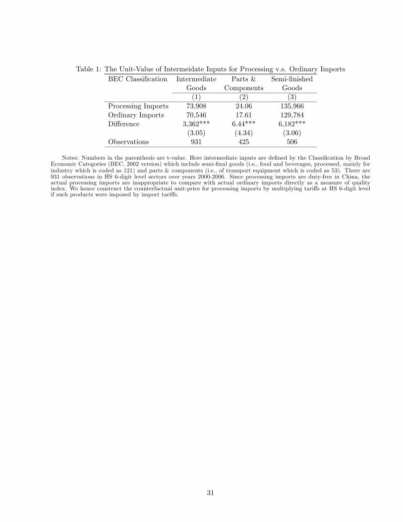
Table 1: The Unit-Value of Intermeidate Inputs for Processing v.s. Ordinary ImportsBEC Classi�cation Intermediate Parts & Semi-�nished

Goods Components Goods(1) (2) (3)

Processing Imports 73,908 24.06 135,966Ordinary Imports 70,546 17.61 129,784Di¤erence 3,362*** 6.44*** 6,182***

(3.05) (4.34) (3.06)Observations 931 425 506

Notes: Numbers in the parenthesis are t-value. Here intermediate inputs are de�ned by the Classi�cation by BroadEconomic Categories (BEC, 2002 version) which include semi-�nal goods (i.e., food and beverages, processed, mainly forindustry which is coded as 121) and parts & components (i.e., of transport equipment which is coded as 53). There are931 observations in HS 6-digit level sectors over years 2000-2006. Since processing imports are duty-free in China, theactual processing imports are inappropriate to compare with actual ordinary imports directly as a measure of qualityindex. We hence construct the counterfactual unit-price for processing imports by multiplying tari¤s at HS 6-digit levelif such products were imposed by import tari¤s.

31

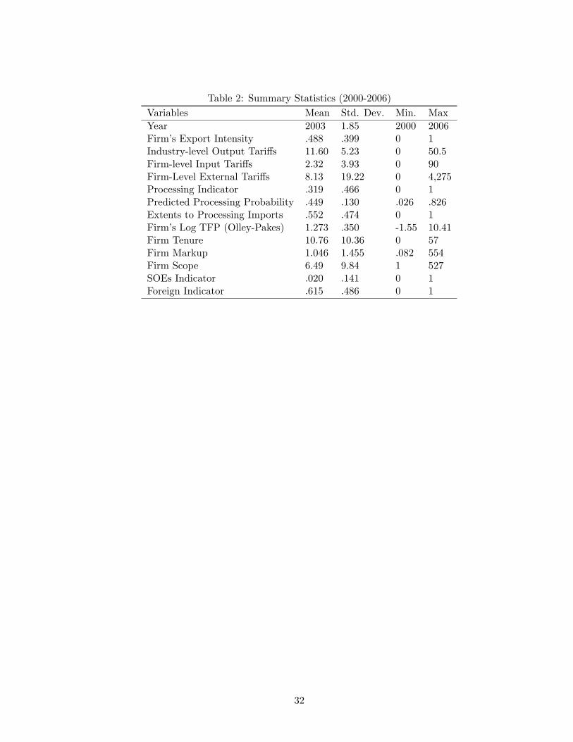
Table 2: Summary Statistics (2000-2006)Variables Mean Std. Dev. Min. MaxYear 2003 1.85 2000 2006Firm�s Export Intensity .488 .399 0 1Industry-level Output Tari¤s 11.60 5.23 0 50.5Firm-level Input Tari¤s 2.32 3.93 0 90Firm-Level External Tari¤s 8.13 19.22 0 4,275Processing Indicator .319 .466 0 1Predicted Processing Probability .449 .130 .026 .826Extents to Processing Imports .552 .474 0 1Firm�s Log TFP (Olley-Pakes) 1.273 .350 -1.55 10.41Firm Tenure 10.76 10.36 0 57Firm Markup 1.046 1.455 .082 554Firm Scope 6.49 9.84 1 527SOEs Indicator .020 .141 0 1Foreign Indicator .615 .486 0 1

32

Table 2: Baseline OLS EstimatesExport Intensity (Exp_int) Full-sample Matched-sample

(1) (2) (3) (4) (5) (6)Industrial Tari¤s .544*** .403* .540*** .012*** .011*** .010**

(98.71) (81.13) (42.91) (59.40) (49.24) (49.24)State-Owned Enterprises -.062*** -.222*** -.163*** -.175***

(-68.42) (-57.63) (-27.39) (-25.57)Foreign Invested Enterprises .308*** .128*** .185*** .140**

(266.5) (75.60) (83.22) (59.92)Obs. Dropped if Exp_int = 0 or 1 No No Yes No No YesObservations 725,993 725,993 172,137 124,618 124,618 87,349R-squared .02 .16 .06 .03 .08 .08

Notes: Robust t-values corrected for clustering at the �rm level in parentheses. *, **, and *** indicates signi�canceat the 10, 5, and 1 percent level, respectively.

33

Table 3: Estimates of Tari¤s Reduction on Firm�s Export IntensityExport Intensity (Exp_int) (1) (2) (3) (4) (5)Industrial Tari¤s 0.0004 -0.0001 -0.0001 -0.0002 0.0001

(1.20) (-0.17) (-0.20) (-0.49) (0.01)Industrial Tari¤s 0.001*** 0.001*** 0.001*** 0.001***�Processing Dummy (2.92) (3.16) (3.11) (3.07)

Firm Input Tari¤s -0.002*** -0.002*** -0.002*** -0.002*** -0.003***(-4.75) (-4.67) (-7.56) (-4.83) (-7.89)

Firm External Tari¤s -0.000 0.000 -0.000 -0.000 -0.000(-1.07) (0.11) (-0.16) (-0.26) (-0.41)

Firm External Tari¤s -0.000* -0.000 -0.000 -0.000�Processing Dummy (-1.92) (-0.44) (-1.16) (-0.88)

Processing Dummy 0.001 -0.013** -0.011** -0.016*** -0.013**(0.25) (-2.27) (-2.19) (-2.71) (-2.33)

State-owned Enterprises 0.019 0.019 0.011 0.017 0.011(0.97) (0.98) (0.69) (0.90) (0.62)

Foreign Invested Enterprises 0.033*** 0.033*** -0.001 0.021* -0.010(2.74) (2.74) (-0.11) (1.65) (-0.84)

Obs. Dropped if Exp_int = 0 No No Yes No YesObs. Dropped if Exp_int = 1 No No No Yes YesYear-speci�c Fixed E¤ects Yes Yes Yes Yes YesFirm-speci�c Fixed E¤ects Yes Yes Yes Yes YesObservations 79,212 79,212 67,086 68,420 56,294R-squared 0.01 0.01 0.01 0.01 0.01

Notes: Robust t-values corrected for clustering at the �rm level in parentheses. *, **, and *** indicates signi�canceat the 10, 5, and 1 percent level, respectively.

34

Table 4: Estimates for Sources of Input Tari¤s VariationExport Intensity Pure Pure Hybrid Switching Firms from

Ordinary Processing Firms pure ord. pure proc. hybrid toFirms Firms to hybrid to hybrid non-hybrid(1) (2) (3) (4) (5) (6)

Industrial Tari¤s -0.000 0.004 0.000 0.001 0.005 -0.000(-0.76) (1.59) (0.68) (0.66) (0.85) (-0.19)

Firm Input Tari¤s -0.002*** -0.044* -0.004** -0.002 -0.001(-5.21) (-1.68) (-2.04) (-0.10) (-0.39)

Firm Input Tari¤s -0.001***(Fixed Tari¤s) (-2.96)

Firm External Tari¤s -0.000 -0.000 0.000 -0.000 -0.001 0.000(-0.50) (-0.79) (0.03) (-0.50) (-0.68) (0.19)

State-owned Enterprises 0.008 0.021 0.014 0.023 � 0.005(0.43) (0.12) (0.47) (0.27) (0.06)

Foreign Invested Enterprises -0.011 0.071 0.029 0.060 0.416** 0.006(-0.66) (1.28) (1.63) (1.37) (2.32) (0.07)

Year-speci�c Fixed E¤ects Yes Yes Yes Yes Yes YesFirm-speci�c Fixed E¤ects Yes Yes Yes Yes Yes YesObservations 31,740 8,063 46,831 12,524 3,644 9,395R-squared 0.01 0.01 0.01 0.01 0.03 0.02

Notes: Robust t-values corrected for clustering at the �rm level in parentheses. *, **, and *** indicates signi�canceat the 10, 5, and 1 percent level, respectively.

35

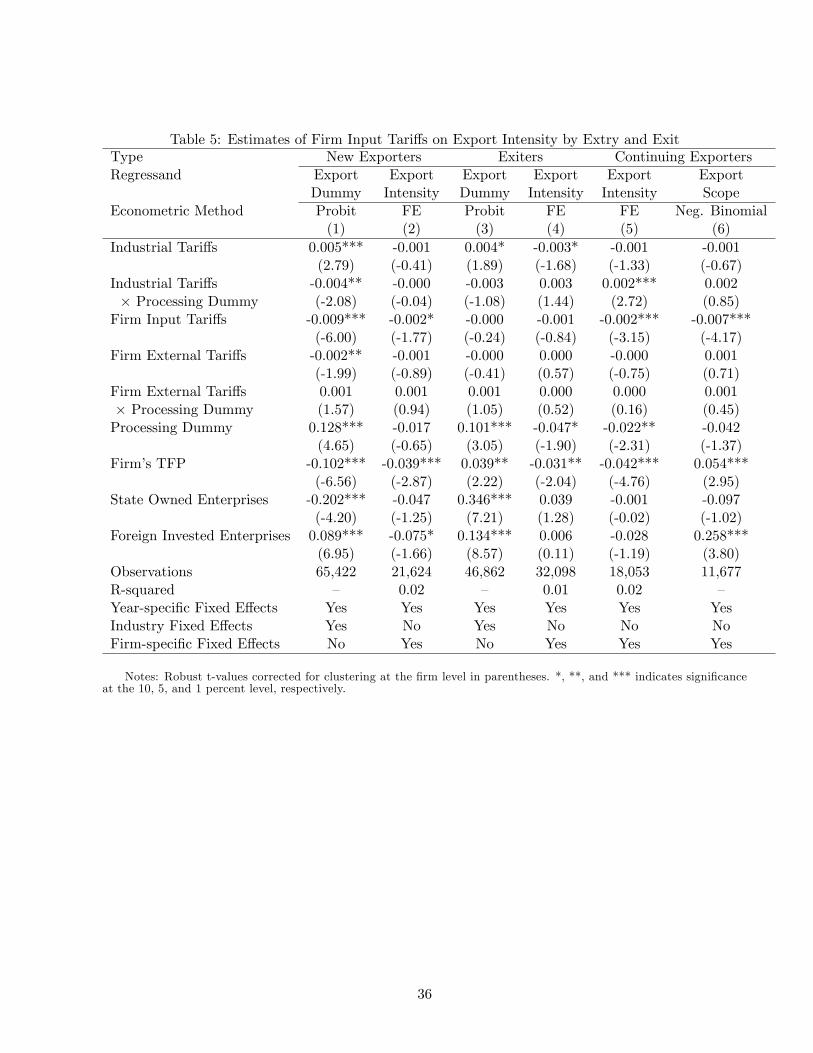
Table 5: Estimates of Firm Input Tari¤s on Export Intensity by Extry and ExitType New Exporters Exiters Continuing ExportersRegressand Export Export Export Export Export Export

Dummy Intensity Dummy Intensity Intensity ScopeEconometric Method Probit FE Probit FE FE Neg. Binomial

(1) (2) (3) (4) (5) (6)Industrial Tari¤s 0.005*** -0.001 0.004* -0.003* -0.001 -0.001

(2.79) (-0.41) (1.89) (-1.68) (-1.33) (-0.67)Industrial Tari¤s -0.004** -0.000 -0.003 0.003 0.002*** 0.002� Processing Dummy (-2.08) (-0.04) (-1.08) (1.44) (2.72) (0.85)Firm Input Tari¤s -0.009*** -0.002* -0.000 -0.001 -0.002*** -0.007***

(-6.00) (-1.77) (-0.24) (-0.84) (-3.15) (-4.17)Firm External Tari¤s -0.002** -0.001 -0.000 0.000 -0.000 0.001

(-1.99) (-0.89) (-0.41) (0.57) (-0.75) (0.71)Firm External Tari¤s 0.001 0.001 0.001 0.000 0.000 0.001� Processing Dummy (1.57) (0.94) (1.05) (0.52) (0.16) (0.45)Processing Dummy 0.128*** -0.017 0.101*** -0.047* -0.022** -0.042

(4.65) (-0.65) (3.05) (-1.90) (-2.31) (-1.37)Firm�s TFP -0.102*** -0.039*** 0.039** -0.031** -0.042*** 0.054***

(-6.56) (-2.87) (2.22) (-2.04) (-4.76) (2.95)State Owned Enterprises -0.202*** -0.047 0.346*** 0.039 -0.001 -0.097

(-4.20) (-1.25) (7.21) (1.28) (-0.02) (-1.02)Foreign Invested Enterprises 0.089*** -0.075* 0.134*** 0.006 -0.028 0.258***

(6.95) (-1.66) (8.57) (0.11) (-1.19) (3.80)Observations 65,422 21,624 46,862 32,098 18,053 11,677R-squared � 0.02 � 0.01 0.02 �Year-speci�c Fixed E¤ects Yes Yes Yes Yes Yes YesIndustry Fixed E¤ects Yes No Yes No No NoFirm-speci�c Fixed E¤ects No Yes No Yes Yes Yes

Notes: Robust t-values corrected for clustering at the �rm level in parentheses. *, **, and *** indicates signi�canceat the 10, 5, and 1 percent level, respectively.

36

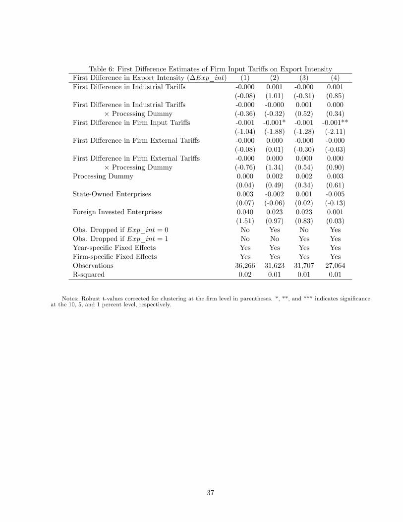
Table 6: First Di¤erence Estimates of Firm Input Tari¤s on Export IntensityFirst Di¤erence in Export Intensity (�Exp_int) (1) (2) (3) (4)First Di¤erence in Industrial Tari¤s -0.000 0.001 -0.000 0.001

(-0.08) (1.01) (-0.31) (0.85)First Di¤erence in Industrial Tari¤s -0.000 -0.000 0.001 0.000

� Processing Dummy (-0.36) (-0.32) (0.52) (0.34)First Di¤erence in Firm Input Tari¤s -0.001 -0.001* -0.001 -0.001**

(-1.04) (-1.88) (-1.28) (-2.11)First Di¤erence in Firm External Tari¤s -0.000 0.000 -0.000 -0.000

(-0.08) (0.01) (-0.30) (-0.03)First Di¤erence in Firm External Tari¤s -0.000 0.000 0.000 0.000

� Processing Dummy (-0.76) (1.34) (0.54) (0.90)Processing Dummy 0.000 0.002 0.002 0.003

(0.04) (0.49) (0.34) (0.61)State-Owned Enterprises 0.003 -0.002 0.001 -0.005

(0.07) (-0.06) (0.02) (-0.13)Foreign Invested Enterprises 0.040 0.023 0.023 0.001

(1.51) (0.97) (0.83) (0.03)Obs. Dropped if Exp_int = 0 No Yes No YesObs. Dropped if Exp_int = 1 No No Yes YesYear-speci�c Fixed E¤ects Yes Yes Yes YesFirm-speci�c Fixed E¤ects Yes Yes Yes YesObservations 36,266 31,623 31,707 27,064R-squared 0.02 0.01 0.01 0.01

Notes: Robust t-values corrected for clustering at the �rm level in parentheses. *, **, and *** indicates signi�canceat the 10, 5, and 1 percent level, respectively.

37

Table 7: Channels of Tari¤s Reduction on Firm�s Export Intensity: Import ScopeRegressand Export Intensity Log Pro�t

(1) (2) (3) (4) (5)Industrial Output Tari¤s -0.000 0.000 -0.000 -0.000 0.011***

(-0.48) (0.09) (-0.86) (-0.90) (3.36)Industrial Output Tari¤s 0.001* 0.001** 0.001* 0.001* 0.000� Processing Dummy (1.93) (2.14) (1.85) (1.71) (0.10)Industrial Output Tari¤s -0.000*** 0.000*** 0.000� Firm Import Scope (-15.76) (3.01) (0.42)Firm Input Tari¤s -0.002*** -0.001*** -0.002*** -0.001*** -0.005*

(-3.91) (-3.20) (-5.72) (-3.60) (-1.65)Firm Input Tari¤s -0.000 -0.000*** 0.000***� Firm Import Scope (-1.19) (-5.36) (2.81)Firm External Tari¤s -0.000 -0.000 -0.000* -0.000 -0.000

(-0.77) (-0.47) (-1.66) (-0.84) (-0.31)Firm External Tari¤s 0.000 0.000 -0.000 -0.000 0.000� Processing Dummy (0.36) (0.34) (-0.55) (-0.10) (0.05)Firm External Tari¤s -0.000 -0.000* -0.000*� Firm Import Scope (-0.15) (-1.78) (-1.69)Firm Import Scope 0.000** 0.001*** 0.000*** 0.000*** 0.003***

(2.17) (9.94) (3.68) (3.33) (4.10)Processing Dummy -0.013* -0.014** -0.011* -0.011* -0.007

(-1.90) (-1.99) (-1.76) (-1.79) (-0.16)State-owned Enterprises 0.018 0.016 0.017 0.017 -0.144

(0.81) (0.73) (0.92) (0.88) (-1.08)Foreign Invested Enterprises 0.018 0.017 -0.015 -0.016 0.142

(1.32) (1.24) (-1.19) (-1.20) (1.56)Firm TFP (Olley-Pakes) -0.024*** -0.023*** -0.046*** -0.046*** 0.599***

(-5.69) (-5.43) (-10.45) (-10.48) (17.94)Observations 65,418 65,418 46,388 46,388 37,407R-squared 0.01 0.02 0.01 0.01 0.06Year-speci�c Fixed E¤ects Yes Yes Yes Yes YesFirm-speci�c Fixed E¤ects Yes Yes Yes Yes Yes

Notes: Robust t-values corrected for clustering at the �rm level in parentheses. *, **, and *** indicates signi�canceat the 10, 5, and 1 percent level, respectively.

38

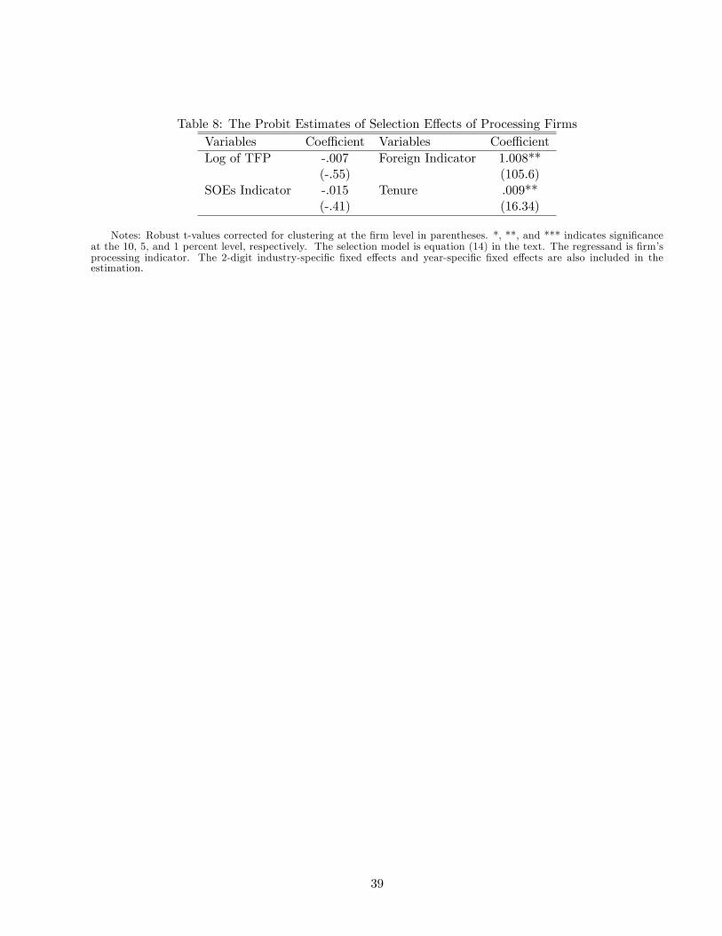
Table 8: The Probit Estimates of Selection E¤ects of Processing FirmsVariables Coe¢ cient Variables Coe¢ cientLog of TFP -.007 Foreign Indicator 1.008**

(-.55) (105.6)SOEs Indicator -.015 Tenure .009**

(-.41) (16.34)

Notes: Robust t-values corrected for clustering at the �rm level in parentheses. *, **, and *** indicates signi�canceat the 10, 5, and 1 percent level, respectively. The selection model is equation (14) in the text. The regressand is �rm�sprocessing indicator. The 2-digit industry-speci�c �xed e¤ects and year-speci�c �xed e¤ects are also included in theestimation.

39

Table 9: Endogenous Choice of Processing FirmsExport Intensity (Exp_int) Processing Probability Extents to Processing

(1) (2) (3) (4)Industrial Tari¤s -0.001 0.000 -0.001 -0.001

(-1.25) (0.00) (-0.80) (-1.00)Industrial Tari¤s 0.004* 0.001 0.001 0.002**� Processing Indicator (1.65) (0.62) (1.04) (2.36)Firm Input Tari¤s -0.002*** -0.002*** -0.003*** -0.003***

(-3.73) (-5.65) (-2.92) (-4.45)Firm External Tari¤s -0.000 -0.000 0.000 -0.000

(-0.87) (-0.75) (0.32) (-0.02)Firm External Tari¤s 0.000 0.000 -0.000 -0.000� Processing Indicator (0.70) (0.64) (-1.56) (-1.27)Processing Indicator 0.214** 0.194** -0.002 -0.007

(2.05) (2.05) (-0.21) (-0.65)State-owned Enterprises 0.018 0.014 0.045 0.037

(0.75) (0.69) (1.19) (1.12)Foreign Invested Enterprises 0.037* -0.016 0.041* 0.003

(1.72) (-0.79) (1.95) (0.16)Firm TFP -0.025*** -0.045*** -0.023*** -0.041***

(-6.10) (-10.55) (-3.93) (-6.56)Firm Tenure 0.001 0.000

(1.13) (0.22)Inverse Mills Ratio 0.124** 0.087**

(2.57) (2.03)Obs. dropped if Exp_int = 0 or 1 No Yes No YesYear-speci�c Fixed E¤ects Yes Yes Yes YesFirm-speci�c Fixed E¤ects Yes Yes Yes YesObservations 65,018 46,042 37,606 26,127R-squared 0.01 0.01 0.01 0.01

Notes: Numbers in paranthesis are t-values. ***(**,*) denotes the signi�cance at 1% (5%, 10%) level.

40

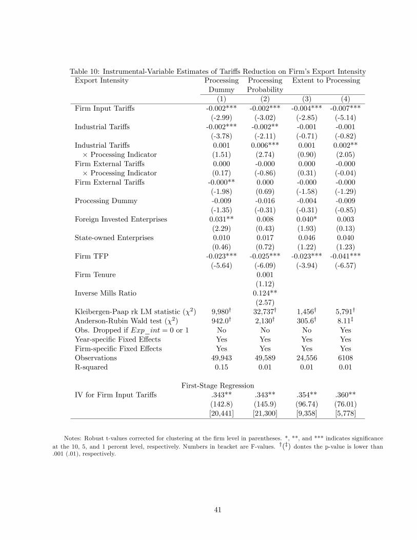
Table 10: Instrumental-Variable Estimates of Tari¤s Reduction on Firm�s Export IntensityExport Intensity Processing Processing Extent to Processing

Dummy Probability(1) (2) (3) (4)

Firm Input Tari¤s -0.002*** -0.002*** -0.004*** -0.007***(-2.99) (-3.02) (-2.85) (-5.14)

Industrial Tari¤s -0.002*** -0.002** -0.001 -0.001(-3.78) (-2.11) (-0.71) (-0.82)

Industrial Tari¤s 0.001 0.006*** 0.001 0.002**� Processing Indicator (1.51) (2.74) (0.90) (2.05)

Firm External Tari¤s 0.000 -0.000 0.000 -0.000� Processing Indicator (0.17) (-0.86) (0.31) (-0.04)

Firm External Tari¤s -0.000** 0.000 -0.000 -0.000(-1.98) (0.69) (-1.58) (-1.29)

Processing Dummy -0.009 -0.016 -0.004 -0.009(-1.35) (-0.31) (-0.31) (-0.85)

Foreign Invested Enterprises 0.031** 0.008 0.040* 0.003(2.29) (0.43) (1.93) (0.13)

State-owned Enterprises 0.010 0.017 0.046 0.040(0.46) (0.72) (1.22) (1.23)

Firm TFP -0.023*** -0.025*** -0.023*** -0.041***(-5.64) (-6.09) (-3.94) (-6.57)

Firm Tenure 0.001(1.12)

Inverse Mills Ratio 0.124**(2.57)

Kleibergen-Paap rk LM statistic (�2) 9,980y 32,737y 1,456y 5,791y

Anderson-Rubin Wald test (�2) 942.0y 2,130y 305.6y 8.11z

Obs. Dropped if Exp_int = 0 or 1 No No No YesYear-speci�c Fixed E¤ects Yes Yes Yes YesFirm-speci�c Fixed E¤ects Yes Yes Yes YesObservations 49,943 49,589 24,556 6108R-squared 0.15 0.01 0.01 0.01

First-Stage RegressionIV for Firm Input Tari¤s .343** .343** .354** .360**

(142.8) (145.9) (96.74) (76.01)[20,441] [21,300] [9,358] [5,778]

Notes: Robust t-values corrected for clustering at the �rm level in parentheses. *, **, and *** indicates signi�canceat the 10, 5, and 1 percent level, respectively. Numbers in bracket are F-values. y(z) dontes the p-value is lower than.001 (.01), respectively.

41

Table 11: Estimates using Firm-Level Tari¤s with Fixed WeightsExport Intensity (1) (2) (3) (4)Industrial Tari¤s 0.000 0.001 0.000 0.002

(0.06) (0.44) (0.06) (0.45)Industrial Tari¤s 0.001 -0.001 0.001 -0.001� Extent to Processing Imports (0.33) (-0.35) (0.32) (-0.37)Firm Input Tari¤s (�xed weights) 0.000 -0.0001* -0.0001 -0.0001*

(-1.56) (-1.78) (-1.59) (-1.83)Firm External Tari¤s -0.000 0.000 -0.000 0.000

(-0.11) (0.06) (-0.07) (0.07)Firm External Tari¤s -0.000 -0.000 -0.000 -0.000� Extent to Processing Imports (-0.09) (-0.20) (-0.13) (-0.21)Extent to Processing Imports 0.084** 0.078* 0.085** 0.080*

(2.38) (1.75) (2.42) (1.78)State-owned Enterprises 0.177** 0.137 0.177** 0.139

(2.00) (1.07) (2.00) (1.08)Foreign Invested Enterprises 0.052* 0.040 0.052* 0.041

(1.81) (1.22) (1.80) (1.23)Firm TFP -0.022** -0.022**

(-2.48) (-2.49)Log Employment 0.015** 0.014*

(2.40) (1.70)Year-speci�c Fixed E¤ects Yes Yes Yes YesFirm-speci�c Fixed E¤ects Yes Yes Yes YesObservations 28,312 22,655 28,312 22,655R-squared 0.01 0.01 0.01 0.01

Notes: Robust t-values corrected for clustering at the �rm level in parentheses. *, **, and *** indicates signi�canceat the 10, 5, and 1 percent level, respectively.

42

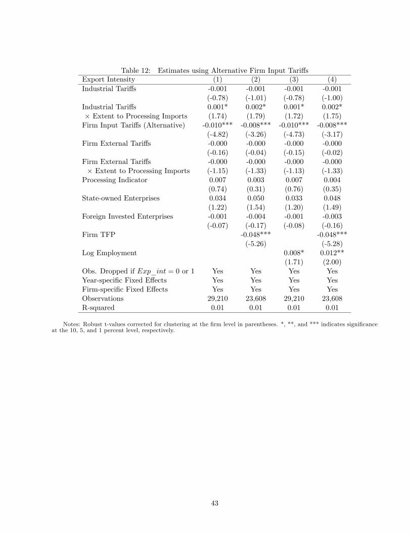
Table 12: Estimates using Alternative Firm Input Tari¤sExport Intensity (1) (2) (3) (4)Industrial Tari¤s -0.001 -0.001 -0.001 -0.001

(-0.78) (-1.01) (-0.78) (-1.00)Industrial Tari¤s 0.001* 0.002* 0.001* 0.002*� Extent to Processing Imports (1.74) (1.79) (1.72) (1.75)Firm Input Tari¤s (Alternative) -0.010*** -0.008*** -0.010*** -0.008***

(-4.82) (-3.26) (-4.73) (-3.17)Firm External Tari¤s -0.000 -0.000 -0.000 -0.000

(-0.16) (-0.04) (-0.15) (-0.02)Firm External Tari¤s -0.000 -0.000 -0.000 -0.000� Extent to Processing Imports (-1.15) (-1.33) (-1.13) (-1.33)Processing Indicator 0.007 0.003 0.007 0.004

(0.74) (0.31) (0.76) (0.35)State-owned Enterprises 0.034 0.050 0.033 0.048

(1.22) (1.54) (1.20) (1.49)Foreign Invested Enterprises -0.001 -0.004 -0.001 -0.003

(-0.07) (-0.17) (-0.08) (-0.16)Firm TFP -0.048*** -0.048***

(-5.26) (-5.28)Log Employment 0.008* 0.012**

(1.71) (2.00)Obs. Dropped if Exp_int = 0 or 1 Yes Yes Yes YesYear-speci�c Fixed E¤ects Yes Yes Yes YesFirm-speci�c Fixed E¤ects Yes Yes Yes YesObservations 29,210 23,608 29,210 23,608R-squared 0.01 0.01 0.01 0.01

Notes: Robust t-values corrected for clustering at the �rm level in parentheses. *, **, and *** indicates signi�canceat the 10, 5, and 1 percent level, respectively.

43

Table 13: Quantile EstimatesExport Intensity OLS Quantile 25% Quantile 50% Quantile 75%Industrial Tari¤s 0.010** 0.010** 0.020** 0.005**

(40.08) (38.26) (45.25) (41.51)Firm Input Tari¤s -0.027** -0.016** -0.052** -0.035**

(-55.35) (-56.49) (-89.1) (-189.2)Firm External Tari¤s -0.0001 -.0000 -0.001** -0.001**

(-1.46) (-0.99) (-10.21) (-8.45)Constant 0.469** 0.0641** 0.479** 0.920**

(120.63) (17.39) (76.47) (568.6)

Notes: Robust t-values corrected for clustering at the �rm level in parentheses. *, **, and *** indicates signi�canceat the 10, 5, and 1 percent level, respectively.

44

1012

1416

Sim

ple 

Ave

rage

 Tar

iffs

.14

.15

.16

.17

.18

Firm

­Lev

el E

xpor

t Int

ensi

ty (F

ull­S

ampl

e)

2000 2002 2004 2006Year

Firm­Level Export Intensity (Full­Sample) Simple Average Tariffs

Figure 1A: Export Intensity against Tari¤s in the Full-Sample Firm Data

2.2

2.4

2.6

2.8

33.

2Fi

rm­S

peci

fic In

put T

ariff

s

.46

.48

.5.5

2.5

4Fi

rm­L

evel

 Exp

ort I

nten

sity

 (Mat

ched

­Sam

ple)

2000 2002 2004 2006Year

Firm­Level Export Intensity (Matched­Sample)Firm­Specific Input Tariffs

Figure 1B: Export Intensity against Tari¤s in the Matched Firm Data

45

Figure 2A: The Distribution of Firm�s Export Intensity in Full-Sample Dataset

05

10D

ensi

ty

0 .2 .4 .6 .8 1exp_int

.51

1.5

2D

ensi

ty

0 .2 .4 .6 .8 1exp_int

kernel = epanechnikov, bandwidth = 0.0310

Kernel density estimate

Figure 2B: The Distribution of Firm�s Export Intensity in Matched-Sample Dataset

46

0.2

.4.6

.81

0 2 4 6 8fit_ind

exp_int_ind Fitted values

Figure 3: Firm Export Intensity against Firm Input Tari¤s

47

0.5

11.

52

2.5

Den

sity

­.5 0 .5residuals

kernel = epanechnikov, bandwidth = 0.0373

Kernel density estimate

Figure 4: Distribution of Residuals

48

0.00

0.20

0.40

0.60

0.80

1.00

Inte

rcep

t

0 .2 .4 .6 .8 1Quantile

0.00

0.01

0.01

0.01

0.02

0.03

ind_

duty

0 .2 .4 .6 .8 1Quantile

­0.0

6­0

.04

­0.0

20.

00fit

0 .2 .4 .6 .8 1Quantile

­0.0

0­0

.00

­0.0

00.

000.

00fe

t0 .2 .4 .6 .8 1

Quantile

Figure 5: The Quantile Estimates of Various Tari¤s Reductions

49

7 Appendix

7.1 Appendix A1: Proof of the Proporsition 1

Since dBrd� = �Ar

S2F

dSFd� < 0;8r = d; x, and �rm�s domestic pro�t is:

�d(') =Eh�(w���'P )��1(1 +B��1d )

(1��)(��1)��1 � f;

we have d�d(')d� = @�d(')

@BddBdd� < 0 since @�d(')

@Bd> 0. Similarly, given �rm�s pro�t at foreign market is:

�x(') =n�1��

�Ef (w

���'P )��1(1 +B��1x )(1��)(��1)

��1 � fx;

we have d�x(')d� = @�x(')@Bx

dBxd� < 0. Therefore a decrease in input trade cost leads to an increase in �rm�s

pro�t.d�(')

d�=d�d(')

d�+d�x(')

d�< 0:

(QED)

7.2 Appendix A2: Proof of the Proporsition 2To show that a decease in �rm input trade costs lead to �rm�s export intensity, we need to showd(1=&)d� > 0. Given

1

�= 1 +

Ehn�1��Ef

1 +B��1d

1 +B��1x

! (1��)(��1)��1

;

we have:

d(1=&)

d�=

Ehn�1��Ef

(1� �)(� � 1)� � 1

1 +B��1d

1 +B��1x

! (1��)(��1)��1 �1

�(� � 1)

��1 +B��1x

�B��2d

dBdd� �

�1 +B��1d

�B��2x

dBxd�

��1 +B��1x

�2 :

Since dBrd� = �Ar

S2F

dSFd� < 0;8r = d; x, we know that d(1=&)d� > 0 is equivalent to:�

1 +B��1x

�B��2d Ad <

�1 +B��1d

�B��2x Ax;

or, 1 +B��1d

1 +B��1x

! 1��1

>AdAx

given Bd=Bx = Ad=Ax from Br = Ar=SF : By simplying, the expression above is equivalent to:

Ax > Ad:

(QED)

50

7.3 Appendix B: Method of Matching Firm and Trade DataAlthough these two data sets have rich information on production and trade, it is challenging to matchthem together. Both data sets contain a variable of �rm�s identi�cation number. But their codingsystems are completely di¤erent and share no any common characteristics. For example, the lengthsof the �rm�s ID variable in transaction-level data set are 10 digits whereas those in �rm-levels onlyhave 9 digits. China�s customs administration just constructs a complete coding system di¤erent fromthe one adopted by the National Bureau of Statistics.

To address this challenge, we use two ways to match transaction-level trade data and �rm-levelproduction data. First, we match two data sets by �rm�s name and year. That is, if a �rm has an exactChinese name in both data sets in a particular year, they should be an identical �rm.9 As a result,the number of matching �rm is 83,679 in total by using the raw production data set, and reduced to69,623 in total by using the more accurate �ltered production data set.

Equally importantly, we then use another matching technique to serve as a supplement. Here werely on two other common variables to identify �rms, namely, zip code and the last seven digits ofa �rm�s phone number. The rationale is that �rms should have di¤erent and unique phone numberswithin a postal district. Although this method seems straightforward, subtle technical and practicaldi¢ culties still remain.10 Therefore, we use the last seven digits of the phone number to serve a proxyfor �rm identi�cation.11

A �rm could miss its name information in either trade or production data set. Similarly, a �rmcould lose information on phone and/or zip code. To secure that our matched data set can covercommon �rms as many as possible, we then include the observations in the matched data set if a �rmoccurred in either the name-adopted matched data set or the phone-and-post-adopted matched dataset. As a result, the number of matched �rms increases to 90,558 when the raw production data setis used, as shown in Column (7) of Table A1. By way of comparison, such a matching performance isin the same magnitude to (or even better than) other similar studies.12 Finally, if we adopt the morerigorous �ltered production data to merge with �rm data, the matched data set ends up with 76,823�rms in total, as shown in the last column of Table A1.

9The year variable is necessary to use for an auxiliary identi�cation variable since some �rms could change their name

in di¤erent years and new comers could possible take their original name.10For example, the phone numbers in the product-level trade data include both area phone codes and a hyphen, whereas

those in the �rm-level production data do not.11This approached is adopted for two reasons: (1) during 2000�2006, some large Chinese cities changed their phone

number digits from seven to eight, which usually added one more digit at the start of the number. Therefore, sticking

to the last seven digits of the number would not confuse the �rm�s identi�cation; and (2) in the original data set, phone

number is de�ned as a string of characters with the phone zip code. However, it is inappropriate to de-string such

characters to numerals since a hyphen bar is used to connect the zip code and phone number. Using the last seven-digit

substring solves this problem neatly.12For example, Ge et.al (2011) used the same data sets and similar matching techniques but ends up with 86,336

matched �rms in total.

51

Table A1: Matched Statistics�Number of FirmsYear Trade Data Production Data Matched Data# of Transactions Firms Raw Filtered w/ Raw w/ Filtered w/ Raw w/ Filtered

Firms Firms Firms Firms Firms Firms(1) (2) (3) (4) (5) (6) (7) (8)

2000 10,586,696 80,232 162,883 83,628 18,580 12,842 21,665 15,7482001 12,667,685 87,404 169,031 100,100 21,583 15,645 25,282 19,0912002 14,032,675 95,579 181,557 110,530 24,696 18,140 29,144 22,2912003 18,069,404 113,147 196,222 129,508 28,898 21,837 34,386 26,9302004 21,402,355 134,895 277,004 199,927 44,338 35,007 50,798 40,7112005 24,889,639 136,604 271,835 198,302 44,387 34,958 50,426 40,3872006 16,685,377 197,806 301,960 224,854 53,748 42,833 59,133 47,591All Year 118,333,831 286819 615,951 438,165 83,679 69,623 90,558 76,946

Notes: Column (1) reports number of observations of HS eight-digit monthly transaction-level trade data from China�sGeneral Administration of Customs by year. Column (2) reports number of �rms covered in the transaction-level tradedata by year. Column (3) reports number of �rms covered in the �rm-level production dataset compiled by China�sNational Bureau of Statistics without any �lter and cleaning. By contrast, Column (4) presents number of �rms coveredin the �rm-level production dataset with careful �lter according to the requirement of GAAP. Accordingly, Column(5) reports number of matched �rms using exactly identical company�s names in both trade dataset and raw productiondataset. By contrast, Column (6) reports number of matched �rms using exactly identical company�s names in both tradedataset and �ltered production dataset. Finally, Column (7) reports number of matched �rms using exactly identicalcompany�s names and exactly identical zip code and phone numbers in both trade dataset and raw production dataset.By contrast, Column (8) reports number of matched �rms using exactly identical company�s names and exactly identicalzip code and phone numbers in both trade dataset and �ltered production dataset.

52

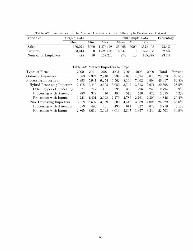
Table A2: Comparison of the Merged Dataset and the Full-sample Production DatasetVariables Merged Data Full-sample Data Percentage

Mean Min. Max. Mean Min. Max.Sales 150,071 5000 1.57e+08 85,065 5000 1.57e+08 25.4%Exports 53,314 0 1.52e+08 16,544 0 1.52e+08 52.8%Number of Employees 478 10 157,213 274 10 165,878 23.7%

Table A3: Merged Importers by TypeTypes of Firms 2000 2001 2002 2003 2004 2005 2006 Total PercentOrdinary Importers 1,659 2,324 2,910 3,931 5,090 4,894 5,070 25,878 35.5%Processing Importers 5,393 5,947 6,254 6,562 8,160 7,602 6,999 46,917 64.5%Hybrid Processing Importers 2,175 2,440 2,695 3,059 3,742 3,613 2,971 20,695 28.5%Other Types of Processing 671 717 181 298 386 296 245 2,794 3.9%Processing with Assembly 283 322 416 482 570 556 426 3,055 4.2%Processing with Inputs 1,221 1,401 2,098 2,279 2,786 2,761 2,300 14,846 20.4%

Pure Processing Importers 3,218 3,507 3,559 3,503 4,418 3,989 4,028 26,222 36.0%Processing with Assembly 353 493 461 490 611 632 679 3,719 5.1%Processing with Inputs 2,865 3,014 3,098 3,013 3,807 3,357 3,349 22,503 30.9%

53

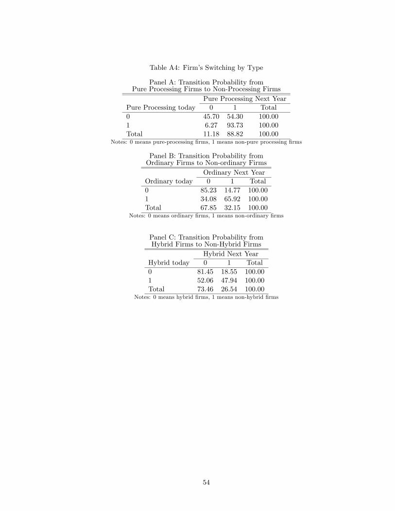
Table A4: Firm�s Switching by Type

Panel A: Transition Probability fromPure Processing Firms to Non-Processing Firms

Pure Processing Next YearPure Processing today 0 1 Total0 45.70 54.30 100.001 6.27 93.73 100.00Total 11.18 88.82 100.00

Notes: 0 means pure-processing �rms, 1 means non-pure processing �rms

Panel B: Transition Probability fromOrdinary Firms to Non-ordinary Firms

Ordinary Next YearOrdinary today 0 1 Total0 85.23 14.77 100.001 34.08 65.92 100.00Total 67.85 32.15 100.00

Notes: 0 means ordinary �rms, 1 means non-ordinary �rms

Panel C: Transition Probability fromHybrid Firms to Non-Hybrid Firms

Hybrid Next YearHybrid today 0 1 Total0 81.45 18.55 100.001 52.06 47.94 100.00Total 73.46 26.54 100.00

Notes: 0 means hybrid �rms, 1 means non-hybrid �rms

54

Appendix Figure 1: Four Types of Chinese Firms

Notes: Dotted lines denote �rms� processing imports/exports whereas real lines represent �rms� non-processingimports/exports.

55

56