Autonomous Robotshttps://doi.org/10.1007/s10514-018-9696-7

Tracking multiple Autonomous Underwater Vehicles

José Melo1,2 · Aníbal C. Matos1,2

Received: 2 May 2016 / Accepted: 12 January 2018© Springer Science+Business Media, LLC, part of Springer Nature 2018

AbstractIn this paper we present a novel method for the acoustic tracking of multiple Autonomous Underwater Vehicles. While theproblem of tracking a single moving vehicle has been addressed in the literature, tracking multiple vehicles is a problemthat has been overlooked, mostly due to the inherent difficulties on data association with traditional acoustic localizationnetworks. The proposed approach is based on a Probability Hypothesis Density Filter, thus overcoming the data associationproblem. Our tracker is able not only to successfully estimate the positions of the vehicles, but also their velocities. Moreover,the tracker estimates are labelled, thus providing a way to establish track continuity of the targets. Using real word data, ourmethod is experimentally validated and the performance of the tracker is evaluated.

Keywords Marine robotics · Position estimation · Underwater robotics · Multiple target tracking

1 Introduction

Autonomous Underwater Vehicles (AUVs) are becoming areliable and cost-effective solution for performing a varietyof underwater tasks in a fully automated way. Among themain tasks to be performed byAUVs are bathymetric surveysand environmental inspections, surveillance and patrolling,or even mine countermeasures operations. The use of suchvehicles means that the assigned tasks can be performed usu-ally in a cost-effective way, but also enables operations inchallenging scenarios that otherwise would not be safe oreven possible for human intervention. While most of thesetasks are traditionally performed using only a single vehi-cle, there are significant research efforts focused towards thedevelopment of algorithms that allow fleets of AUVs, navi-gating in a coordinated fashion, to achieve a common goal.

The use of multiple vehicles allows the parallelization oftasks that otherwise would not be possible, thus reducingoperations time. The potential for efficiency gains is evengreater if the various vehicles are collaborating for the com-pletion of a task. The use of teams of collaborating AUVs has

B José Melojose.melo@fe.up.pt

Aníbal C. Matosanibal@fe.up.pt

1 Faculty of Engineering, University of Porto, Rua Dr. RobertoFrias, s/n, 4200-465 Porto, Portugal

2 INESC TEC, Rua Dr. Roberto Frias, 4200-465 Porto, Portugal

been foreseen for different applications, for example minecounter-measures missions (Prins and Kandemir 2008) orarchaeological missions. Even though there is an extensiveand growing literature on cooperative control theory, thereare only a few approaches demonstrating complete multi-AUV cooperation in field trials in water. An example ofthis would be the efficient mapping of a given area usingmultiple vehicles, addressed in (Paull et al. 2015). Teamsof cooperating AUVs have also been reported to performadaptive environmental sampling tasks, namely by havingmultiple vehicles performing plume tracking quickly andwith high temporal and spatial resolution (Schulz et al. 2003).In a somewhat similar mission, sea trials with a fleet often autonomous underwater gliders deployed as an adaptive,coordinated ocean sampling network have also been reported(Fiorelli et al. 2006; Leonard et al. 2010). Within the frame-work of environmental sampling, a distributed multi-vehiclepatrolling approach was also proposed (Marino et al. 2015).

With such developments, it is reasonable to expect that ina near future new applications will arise requiring the opera-tion of multiple AUVs concurrently, cooperating to achievea desired goal. With the increase of such multi-vehiclemissions of underwater vehicles, the problem of trackingmultiple AUVs in real-time becomes even more relevant. Infact, for most of the classical missions for AUVs, the abilityto track the vehicles during operation time is not only desir-able, but even critical for some more uncertain hazardousscenarios, such as the military or oil industry applications.

123

Autonomous Robots

Tracking AUVs can be done by listening to the acousticsignals exchanged between the vehicle and a set of acousticbeacons deployed in the area of operations. The AUVs needto emit an acoustic signal, that is then detected by each one ofthe beacons at different times, and according to their distanceto the vehicle. By combining the Time-of-Flight (ToF) of thesignals as detected by the beacons, the position of a vehiclecan be computed by using multilateration techniques.

From the majority of the literature considering trackingof AUVs, only a few have been able to fully address theproblem of tracking multiple vehicles. In fact, only seldomscenarios with multiple targets are considered and experi-mentally validated. The main obstacle in such cases is theability to uniquely associate acoustic signals with the sourcethat emitted such signals. Tracking more than one vehicleusually requires that each one of the vehicles emits signalsthat can be easily distinguishable between each other. A natu-ralway to complywith this requirement is to have the vehiclesusing different frequency modulated signals. Alternatively,time-division multiplexing schemes can also been derived.While these approaches are proven, they are far from beingoptimal.

Actually, both options are hardly scalable, particularlywhen addressing situationswith several vehicles. This is evenmore striking if, as frequently happens, the acoustic beaconsare also required to emit their own acoustic signals, in orderto provide navigational aids to the vehicles. When using timemultiplexing schemes, time slots are attributed to each one ofthe devices operating on the network, so they can emit acous-tic signals. For operations withmultiple vehicles, the numberof time slots is increased,which in turn also increases the timeinterval between two consecutive signal emission slots for agiven vehicle. As the number of vehicles increases, this cansignificantly degrade the performance of the trackers. On theother hand, resorting to different frequency signals is alsonot a scalable approach. Increasing the number of distinctfrequency signals is cumbersome and costly as it requires thedevelopment of specific hardware for emission and detectionof the signals. This is even more complicated if we considerthat the acoustic signals used are usually in a very confinedband, approximately between around 10 to 30 kHz, which inturn limits the number of available frequencies.

1.1 Contribution

It can be argued that standard tracking algorithms, such asKalman Filter based trackers, would be an appropriate solu-tion for tracking multiple vehicles, as in the multiple AUVcooperative scenarios that have been mentioned. In fact, formost of the cases the number of vehicles in operation isknown in advance, so it could be just the case of runningmul-tiple trackers in parallel.However, as itwasmade clear above,it is often challenging to have multiple vehicles emitting

easily distinguishable acoustic signals. Therefore, in suchscenarios standard tracking approaches would require, andstruggle, with complex data-association methods.

In this article we are focused on a different approach tothe problem of tracking multiple AUVs. In specific, we aretrying to address the problem of tracking multiple AUVsthat emit similar acoustic signals, which are not possible todistinguish between each other. The main contribution ofthis paper is then the derivation of a suitable algorithm foracoustically tracking multiple AUVs that can cope with suchlimitations. The proposed tracker, which is based on a Prob-ability Hypothesis Density (PHD) filter, doesn’t require anydata association step, which means that it can estimate thepositions and velocities of the different vehicles, even whenthey are emitting similar and otherwise undistinguishableacoustic signals. Besides that, an experimental validation ofthe proposed approach is also provided. Up to the authorsknowledge, it is the first time that such an approach has beenpresented.

The work here presented is in fact an extension of aprevious conference article (Melo and Matos 2014). Thatwork was a preliminary study concerning the feasibility ofusing Random Finite Sets to address the problem track-ing multiple AUVs. In a simulation environment, a PHDfilter was considered for the problem of tracking threeunderwater autonomous vehicles using range-only acousticmeasurements detected by an Long baseline (LBL) acous-tic positioning network. Nevertheless that preliminary studywas limited, in the sense that it did not fully address all thechallenges of a realistic underwater AUV operations. Forexample, in the simulations presented all the vehicles had thesame known and constant velocity, and only followed trajec-tories with a constant heading. These are obvious limitingassumptions. Moreover, multipath acoustic phenomenons,commonly observed in acoustic underwater communica-tions, were not part of the simulation environment. At thesame time, the proposed tracker had a tendency to overesti-mate the number of vehicles, which could potentially lead toincorrect target estimates. In what follows we will addressthese shortcomings of the initial approach.

In the work here presented there are no assumptions con-cerning the velocity or trajectory of the vehicles. One ofthe other major contributions of the work here presented isa suitable labelled formulation of the multitarget trackingproblem, which enables the tracker to provide a full indi-vidual trajectory history of each of the individual targets.Another feature of interest provided is the ability to grace-fully address situations with an unknown and time-varyingnumber of targets. This is in fact a scenario that can be eas-ily envisioned for future multi-vehicle operations, but it isnot usually addressed by the traditional vector-based targettracking approaches. Another contribution here proposed isthe derivation of a suitable deghosting heuristics that is able

123

Autonomous Robots

to deal with the emergence of ghost targets, as it will bemade clear in the sections ahead. Finally, this article will alsoprovided the experimental validation of the proposed algo-rithms, demonstrating the robustness of the tracker when inthe presence of measurement ambiguity that characterizesunderwater acoustic signals.

1.2 Organization of the paper

The paper proceeds as follows. Section 2 provides a review ofwork related to the topic of acoustic underwater target track-ing. In Sect. 3 the single target tracking case is introduced.Details of the Finite Set Statistics framework that will beused, and derivation of the labelled Sequential Monte Carloimplementation of the PHD filter can be found, respectively,in Sects. 4 and 5. Section 6 details the experimental setupused to obtain data and validate this approach, while Sect. 7presents the results obtained. Finally, in Sect. 8 we discussthe attained results and present some final remarks.

2 Related work

In this article we are focused on the problem of tracking mul-tiple AUVs, which is of relevance for the majority of AUVoperations. In this section we provide a brief state-of-the-artreview of the topic of acoustic tracking of AUVs. However,tracking of AUVs can also be considered as part of the big-ger, more general and broader area of tracking underwateracoustic sources. Research in this area has been investigatedin other areas other than the AUV community, for example inthe area ofUnderwaterWireless SensorNetworks (UWSNs).This will also be reviewed in this section. Nevertheless, thevast majority of the research so far has considered only thesingle target scenario.

TrackingofAUVs is perhaps themostwell knownapplica-tionof underwater target tracking for the robotics community.The methods for tracking a single vehicle are well estab-lished and have been fairly addressed in the literature. On itsessence, they all rely on computing the position of the vehiclefrom a set of acoustic ranges or bearings between a vehicleand a set of beacons, deployed at predefined fixed locations,whether at the surface or at the bottom of the sea. Examplesof AUV tracking are found for instance by Watanabe et al.(2009), on which an accurate tracking method to estimatethe position of AUV relative to a mother ship is described,using a Super-Short Baseline Navigation acoustic network.On the other hand, Melo and Matos (2008) demonstrate howtracking an AUV can be performed with an Inverted LongBaseline Navigationmethodwith only two acoustic beacons.In line with the vast majority of the literature, both the ref-erences only address the problem of tracking a single AUV.Some commercially available AUV tracking systems pro-

vide a way for simultaneously track multiple vehicles. Oneexample of this is the ATACS system (Odell et al. 2002),which uses an identifier code transmitted with each signal,thus overcoming the problem of data association. This how-ever, requires the existence of a data link between the nodesin the acoustic network. A different alternative is adopted bythe GAPS systems (Napolitano et al. 2005), whichmakes useof different frequency modulated acoustic signals to be ableto uniquely identify each of the nodes in the network.

Though not exactly the problem of tracking multiplevehicles, some closely related problems are also worthmentioning. For example, the problem of localizing mul-tiple underwater acoustic sources using AUVs have beenaddressed in the literature. Choi and Choi (2015) addressthe problem of using a manoeuvring AUV equipped withseveral hydrophones to detect multiple acoustic sources, butconsiders only the case of a constant and known number ofsources. Braca et al. (2014) propose the use ofmultipleAUVsas sensor nodes of a multistatic surveillance reconfigurableacoustic network with the purpose of detecting underwatertargets in anti-submarine warfare environments. The use ofUWSNs for acoustic tracking of underwater manoeuvringtargets has also been addressed (Zhang et al. 2014; Wanget al. 2012). However, often the authors only consider thesingle target case.

2.1 Tracking of multiple targets

Only a few authors addressed problems of tracking mul-tiple underwater targets, that are closely related to theone here in analysis. The problem of Multitarget Trackingin both multistatic active and passive sonobuouy systemshas been addressed by Georgy et al. (2012), Georgy andNoureldin (2014). The authors detail a solution that is ableto track an unknown time-varying number of multiple tar-gets and keeping continuous tracks, in scenarios that dependon either bearing observations only, or both bearing andDoppler observations. Both papers present extensive simu-lation results, for scenarios with sixteen stationary receiversand two moving targets. On top of that, in the former, exper-imental results were also presented. The performance ofseveral other multitarget trackers has also been assessedin similar environments, namely the Multi Target Tracker(MTT) (Lang et al. 2009) and a Gaussian-Mixture Cardi-nalized Probability Hypothesis Density Filter (GM-CPHD)(Georgescu et al. 2009; Erdinc et al. 2008), among others.In terms of the tools used, the latter work is closely relatedto the approach here proposed. In fact these two referencessharewith the presentwork the use of algorithms based on theRandom Finite Set (RFS) framework developed by Mahler(2008). Nevertheless, the underlying problem under studywas the use of Multi-static sonar data for tracking a singlemoving source.

123

Autonomous Robots

Morelande et al. (2015) presented a method for detec-tion and tracking of multiple underwater targets, in this caseusing a Sequential Monte Carlo (SMC) approximation oftheMultiple Hypothesis Tracker (MHT), but only simulationresultswere presented.Kreucher and Shapo (2011) describeda surveillance application on which a passive acoustic sen-sor array is used to monitor a given surveillance region anddetect and trackmoving targets in the two dimensional space.The paper described a strategy to track multiples target usingonly bearing acoustic data frommultiple passive arrays. First,a fixed discrete grid method is used for detection, while aparticle filter is later used for tracking, This rather uniqueapproach has been demonstrated using both simulated andreal data. Despite its merits, the proposed Bayesian approachtreats the problem, both conceptually and in implementation,as separate tasks of estimating the target present probabilityand the estimating target state probability. Moreover, aspectslike missed detections and disappearing targets are not con-sidered. Considering that, the present work proposes to usea RFS based approach, that is able to address those issues.Moreover, the detection and tracking problems are consid-ered in an integrated way.

3 Tracking a single AUV

The scenario under analysis in this section is the one of track-ing a single vehicle when using an LBL based system. Thisis done for the sake of clarity, as the concepts here presentedalso hold for the case of tracking multiple vehicles. In theremainder of this section we will briefly describe the work-ing principles of LBL networks, and present the motion andsensor models used for the single target tracking problem.However, the interested reader should refer for example to thework by Melo and Matos (2008), and the references therein,for more depth in the topic.

Tracking an AUV requires it to be active, meaning that thevehicle needs to emit acoustic signals in order to be detected.The acoustic signals emittedby theAUVwill thenbedetectedby each of the acoustic beacons that compose the LBL acous-tic network. LBL systems are one of the most robust, reliableand accurate configurations of Acoustic Navigation systems,and used in some of themost challenging scenarios, typicallyin the military and oil industries. Comparing to their counter-parts, one of the main advantages of LBL systems is that theycover a relatively wide area and have very good, depth inde-pendent, position accuracy, which falls in the meter scale.

LBL systems need to have an array of acoustic beaconsdeployed on the seafloor, in specific predefined fixed loca-tion within the operation area. Alternatively, to overcomethe need of deploying the beacons on the seafloor, the use ofGPS-enabled intelligent buoys has been proposed, in a con-figuration called Inverted LBL.With the use of such systems,

Fig. 1 Schematic view of and Inverted LBL setup for tracking multipleAUVs

the transponders of the bottom are replaced by floating buoyswhich carry the acoustic transducers, as exemplified in Fig. 1.Due to the fact that such devices also carry Global Naviga-tion Satellite Systems (GNSS) receivers, calibration of suchbeacons can be significantly simplified. On the remainder ofthis article the focus will be on using GNSS enabled buoys asacoustic beacons. A detailed review of the different AcousticNavigation schemes, their individual strengths and their dis-advantages has been provided for example by Peñas (2009).

For the general case four beacons need to be deployed, inorder to obtain the three dimensional position of the vehi-cle. However, under some specific conditions, for examplewhen operating at shallow water and depths relatively smallwhen comparing to the length of the baseline, this numbercan be smaller, as described by Melo and Matos (2008). Inthe remainder of this section we will only consider a setof two acoustic beacons, in an Inverted LBL configuration.Therefore, only the horizontal position of the AUV will beof interest.

With this setup, it is possible to directly compute rangesto each of the beacons from the ToF of the signals that eachof the beacon detects. Figure 2 illustrates the scenario justdescribed. The distances d1 and d2, which are, respectively,the slant ranges from the AUV to beacon 1 and beacon 2, areeasily obtained from the time-of-flight of the acoustic signals.Then the position of the AUV can then be computed, bysimple triangulation or multilateration of the ranges betweenthe vehicle and all the beacons.

3.1 Target and sensor model

The system that was just described consists of an AUV nav-igating and periodically emitting an acoustic signal. Thesesignals are detected by the two acoustic beacons, and thenconverted to range observations of the vehicle. Such scenarioconfigures a typical target tracking scenario. The behaviourof the whole system can be described by the means of thesingle target dynamical model, fk and the single target mea-surement model h_k, (1) and (2), respectively.

xk = fk(xk−1, vk−1) (1)

zk = hk(xk,nk) (2)

123

Autonomous Robots

Fig. 2 Schematic view of the setup required for tracking AUVs usingan LBL acoustic network

In the equations above, xk refers to the state vector ofa target. It is usually considered that the interesting statevariables to be estimated are the vehicle’s horizontal positionand velocity. The state vector xk can then be defined as:

xk = [xk yk xk yk

]T(3)

Naturally, xk and yk denotes the position of the vehicle whilexk and yk refer to the vehicle’s velocity. It is further assumedthat the dynamic model of the target follows a Gaussian con-stant velocity model, according to (4).

⎡

⎢⎢⎣

xk+1

yk+1

xk+1

yk+1

⎤

⎥⎥⎦ =

⎡

⎢⎢⎣

1 0 Δ 00 1 0 Δ

0 0 1 00 0 0 1

⎤

⎥⎥⎦

⎡

⎢⎢⎣

xk

yk

xk

yk

⎤

⎥⎥⎦ + vk (4)

In the equation above Δ is the sampling interval and vk ∼N (0, Q) is the white Gaussian process noise, with matrixQ the process noise covariance. On a given sampling periodinterval, each of the acoustic beacons produces one rangeobservation of the target, that is related with the state vectorxk according to the measurement equation:

zk,i = hi (xk) + nk,i (5)

hi is the real valued function responsible for computing theexpected range between the vehicle current position, and thelocation of each beacon, (x0,i , y0,i ), and nk,i ∼ N (0, σi )

is the measurement noise associated with acoustic beacon i ,assumed to be Gaussian:

hi (xk) =√

(xk − x0,i )2 + (yk − y0,i )2 (6)

A Bayesian estimation method is employed to estimatethe position of the vehicle from the rangemeasurements. Dueto the non-linearity of the range measurements with respect

to the system state, an Extended Kalman Filter is the mostcommonly used. However, the use of an Unscented KalmanFilter or even a Particle Filter would also be suitable.

Because the range observations are naturally noisy, withreflections and multipath phenomenons being detected bythe acoustic transducers, outlier rejection strategies need tobe employed. For this purpose, measurement gating can bedone by comparing incoming ranges with normalized inno-vation squared (Matos et al. 1999; Fulton et al. 2000). Arange measurement is only considered valid if

νT S−1ν < γ (7)

where ν = [zk − Fxx ] is the innovation vector and S−1

corresponds to the innovation covariance matrix. The param-eter γ is given by an appropriate χ2 distribution, and it canbe easily recovered from a distribution table for the desiredconfidence level. Alternatively, a suitable value can also beempirically determined.

Extending the single target case to accommodate the pres-ence of multiple targets is not straightforward, mostly dueto the difficulty of correctly distinguishing and associatingacoustic signals emitted from each vehicle. In the next sec-tion we introduce the Random Finite Set framework, withwhich will be used to address exactly this problem.

4 RFS and the PHD filter

Multi-object filtering applications, such as the problem oftracking multiple vehicles, have been widely addressed, par-ticularly by the radar tracking community. The objective ofmulti-object filtering is to jointly estimate the number ofobjects and their states from a set of observations. Both theMultiple Hypothesis Tracking (MHT) and the Joint Prob-abilistic Data Association (JPDA) have been presented inthe literature as classical approaches for this problem (Bar-Shalom and Li 1995; Stone et al. 2013). However, thesetraditional algorithms, rooted on theBayes filtering paradigmpresent a number of pitfalls when addressing such scenarios.

Being based on the Kalman Filter, these algorithms relyon a vector representation, which requires stacking states andmeasurements from the different targets. This is not a satis-factory representation when both the number of targets andmeasurements are random and varying. Additionally, a dataassociation step, on which an explicit associations betweenmeasurements and targets is established, is required, whichcan be computationally very demanding, or even intractable.

An alternative formulation for the multiple target estima-tion problem, and one that only recently emerged, can beachieved by using random set theory to formulate the gen-eralmultisensormultitargetBayes filter.On such approaches,both the collection of individual targets states and the collec-

123

Autonomous Robots

Fig. 3 Illustration the basic concept of FISST theory, according towhich the multisensor-multitarget problem is transformed in a single”meta sensor - ”meta target” problem (Granstrom et al. 2014)

tion of measurements are modelled as RFS, to obtain a setvalued version of the general Bayes Filter. Loosely speak-ing, a RFS can be though of as a probabilistic representationof a collection of spatial point patterns that accounts foruncertainty in both the number of objects and their spatiallocations. The usage of random finite sets, opposed to ran-dom vectors, is a more suitable formulation for addressingvarying number of targets, target (dis)appearance and spawn-ing, the presence of clutter and association uncertainty, falsealarms and missed detections or even extended targets.

Developed by Mahler, the Finite Set Statistics framework(FISST) is a unified framework for data fusion based onrandom set theory, a geometrical and mathematically simpli-fied version of point process theory. FISST provides a set ofmathematical tools that allow direct application of Bayesianinferencing to multi-target problems (Vo et al. 2005). Theaim of FISST is to transform multisensor-multitarget prob-lems into single-sensor single-target problems, by bundlingall sensors into a single ”meta-sensor“, all targets into asingle ”meta-target“ and all observations into a single ”meta-observation“ (Mahler 2013). This is illustrated in Fig. 3.In that way, it is possible to construct true multisensor-multitarget likelihood functions and true multitarget Markovtransition densities from the motion models and measure-ment models of individual targets and sensors.

4.1 Random finite set formulation of multitargetfiltering

Analogously to the traditional recursive single target BayesFilter, the multisensor-multititarget Bayes Filter propagatesthe multitarget Bayes posterior density pk(Xk |Z1:k) distribu-tion through time, conditioned on the sets of measurementsup to time k, Z1:k , using the traditional prediction-updaterecursion as follows,

p(Xk |Z1:k−1) =∫

p(Xk |X)p(Xk−1|Z1:k−1)δX (8)

pk(Xk |Z1:k) = p(Zk |Xk)p(Xk |Z1:k−1)∫p(Zk |Xk)p(Xk |Z1:k−1)δX

(9)

where the integrals present are set integrals, as introduced bythe FISST framework.

In the recursion above (8) is the prediction step, while (9)is update step. Both the multitarget state transition function,p(Xk |X) and the multisensor likelihood function p(Zk |Xk)

can be derived from the underlying single target singlesensor and physical models using FISST techniques. Eventhough the general multisensor-multitarget Bayes filters inintractable for the general case, with the use of appropriatecalculus tools introduced by FISST, it is possible to deriveapproximations, such as the Probability Hypothesis DensityFilter.

Both the set of tracked objects Xk and the set of observa-tions received Zk at instant k are modelled as random finitesets. It should be noted that, conversely to standard single-target filtering, the dimensions of the random finite sets Xk

and Zk in the recursion (8–9) can vary with time.

Xk = {xk,1, . . . , xk,MX(k)} (10)

Zk = {zk,1, . . . , zk,NZ(k)} (11)

In (10) MX(k) refers to the number of targets at instant k,while NZ(k) in (11) refers to the the number of observationsat the same instant.

The set of targets being tracked at a given time instant,Xk ,is composed by the collection of targets that survive from theprevious time step, Sk|k−1, together with the collection ofspawned targets, Bk|k−1, and the collection of new targetsappearing only the in current time step, �k .

Xk =⎛

⎝⋃

x∈Xk−1

Sk|k−1(x)

⎞

⎠∪⎛

⎝⋃

x∈Xk−1

Bk|k−1(x)

⎞

⎠∪�k (12)

Similarly, the set of observations received at a giventime instant (13) is a collection of both the measurementsobserved due to the present targets, Θk , which also includesthe probability of a missed detections, together with cluttermeasurements Kk corresponding to false alarms that mayexist in that time instant.

Zk = Kk ∪⎛

⎝⋃

x∈Xk

Θk(x)

⎞

⎠ (13)

In fact, using randomfinite sets formodelling themultitar-get state (12) and themultitargetmeasurements (13) providesan easyway to address target birth and spawning, or even highdensity of clutter measurements.

4.2 PHD filter

The Probability Hypothesis Density (PHD) Filter, initiallyproposed in Mahler (2003), is perhaps the most popular

123

Autonomous Robots

approximation to the optimal Bayesian multitarget filter.Instead of propagating the full posterior (9), the PHD fil-ter propagates only the first-order statistical moment of theobjects RFS of the objects. In a way, the PHD filter canbe considered the multitarget counterpart of the constantgain Kalman Filter, that also only propagates the first ordermoment of a distribution.

Some assumptions must be observed in order to makethe aforementioned propagation tractable, namely the sig-nal to noise ratio (SNR) has to be high and all the targetsshould move independently of each other. The detection andmeasurement of a target is also assumed to be independentof other targets. Moreover, the PHD filter assumes that theRFS are Poisson RFS, one of the simplest class of RFS. Theintensity function, also known in the tracking literature as theProbability Hypothesis Density, completely characterizes aPoissonRFS, thus the name of the filter. The interested readershould refer to Vo et al. (2005); Vo and Vo (2013) and thereferences therein for a theoretical insight on the foundationsof the PHD filter.

A probability hypothesis density function is completelycharacterized by the property in (14), which means that inte-grating a given PHD function Dk over and entire region Sgives the expected number of objects in that region, Nk|k .Additionally, the peaks of Dk identify the likely position ofthose objects:

∫

SDk|k(X|Z(k))dX = Nk|k (14)

It should be noted that, as before, the integral present aboveis a FISST derived set integral.

The PHD filter consists on two equations: the predictorequation and the corrector equation, as follows. While thePHDfilter predictor Eqs. (15–16) allow the current PHD to bepredicted and extrapolated, the corrector equations (17–18)allow the predicted PHD to be updated with the observations(Mahler 2008).

Dk|k−1(xk |Z1:k−1) = γk(xk)

+∫

φk|k−1(xk−1)Dk−1|k−1(xk−1|Z1:k−1)dxk−1 (15)

φk|k−1(xk−1) = pS,k(xk−1) fk|k−1(xk |xk−1) (16)

In the prediction equations above, pS,k refers to the proba-bility a given target has to survive, from one time step to thefollowing, fk|k−1 refers to the single target state transitiondensity, and γk refers to the intensity of spontaneous births.

Dk|k(xk |Zk) = ΞZk (xk)Dk|k−1(x|Zk−1) (17)

ΞZk (xk) = (1 − pD,k) +∑

z∈Zk

ψk,z(x)Kk + 〈Dk|k−1, ψk,z(x)〉

(18)

In the corrector equations above pD,k is the probability ofdetection of a target. Kk refers to the false alarms cluttermodel, and 〈·,·〉 denotes the usual inner product. Addition-ally,

ψk,z(x) = pD,k g(z|x) (19)

with g(z|x) being the single target likelihood function.

4.3 The sequential Monte Carlo PHD (SMC-PHD)filter

A closed formed solution for the PHD filter (15–18) has beenderived by Vo et al. (2005). This filter, the Gaussian MixturePHD filter (GM-PHD) admits only scenarios on which thetargets evolve and generates observations independently, andfollow a linear gausian dynamical model. Additionally, is isalso assumed that the sensors follow linear and Gaussianmeasurement models. Recalling the single target scenariodescribed in Sect. 3, there are non-linearities present in themeasurement model (2), thus this is not a suitable approach.Because of that, an approximation to the PHDfilter recursionis more adequate.

The Sequential Monte Carlo PHD filter is an approx-imation to general PHD recursion that, analogously tostandard Particle Filters, uses randomly distributed particlesto approximate the density functions that represent the PHDpredictor and corrector equations. For that reason, anotherpossible designation for the SMC-PHD is Particle PHD fil-ter. In fact, for the case when there is only one target with nobirth, no death, no clutter and unity probability of detection,the PHD filter reduces to the standard particle filter.

Considering the particle approximation, the PHD pre-dictor equation can be rewritten as in (20), where theapproximation is done with Lk−1 particles, correspondingto the RFS containing the surviving targets, and Jk new par-ticles introduced, representing the RFS of the birth targets.For the general case the birth particles should cover the entirespace of observation however, it is often the case that the priorknowledge regarding the location where possible new targetsmay appear is incorporated.

Dk|k−1(xk) =Lk−1+Jk∑

i=1

wk|k−1δx(i)k−1

(x) (20)

where

xk|k−1 ∼{

qk(.|xk−1,Zk), if 1 ≤ i ≤ Lk−1

pk(.|Zk), if Lk−1 < i ≤ Lk−1 + Jk

(21)

123

Autonomous Robots

and

wk|k−1 =

⎧⎪⎨

⎪⎩

φk|k−1(xk−1)

qk(x(i)k |x(i)

k−1,Zk )wk−1, if 1 ≤ i ≤ Lk−1

γk (x(i)k )

Jk pk (x(i)k |Zk )

, if Lk−1 < i ≤ Lk−1 + Jk

(22)

where qk(.|xk−1,Zk) and pk(.|Zk) are two importance sam-pling proposal densities for the surviving and new bornparticles, respectively.

In the same way, the SMC approximation for the PHDcorrector can be rewritten as in (23):

Dk|k(xk) =Lk−1+Jk∑

i=1

wk|kδx(i)k−1

(x) (23)

where

wk|k =⎡

⎣(1 − pD(x(i)

k ))+

∑

z∈Zk

pD(x(i)k )gk(zk |xk)

Kk +ck(z)

⎤

⎦wk|k−1

(24)

Kk refers to the intensity of the clutter measurement RFS and

ck =Lk−1+Jk∑

i=1

pD(x(i)k )g(zk |xk)wk|k−1. (25)

The particle transition density fk|k−1(xik |xi

k−1) and mea-surement likelihood g(zk |xk) are obtained reusing the pre-viously derived single target dynamical model (4) andmeasurement model (5), respectively. However, it should benoted that the measurement gating strategy adopted for thesingle target case (7) is not needed. Further details on thederivation and convergence properties of the SMC-PHD fil-ter can be found in (Vo et al. 2005; Clark 2006)

Following the prediction and correction stages of theSMC-PHD filter, and analogously to what happens with thestandardparticle filter, there is a need to resample the particlesin order to prevent sample impoverishment. Though differ-ent resampling strategies can be applied, such as stratifiedsampling or residual sampling, there is a common prefer-ence towards the use of systematic resampling, since thisalgorithm is easy to implement, has a linear computationalcomplexity and, from a uniform distribution perspective, istheoretically superior (Hol et al. 2006).

The resampling stage of the SMC-PHD filter differs onlyfrom the traditional resampling strategies adopted in standardparticle filters in that in the PHD filter the weights are not

normalized to sum up to one, but instead,to the total particlemass Nk|k (Clark 2006), where

Nk|k =Lk−1+Jk∑

i=1

w(i)k|k (26)

Because in the prediction stage of the algorithm there arealways a number Jk of birth particles that are introduced, thenumber of particles is always increased on every time stepof the filter. Therefore, in the resampling stage of the PHDfilter the number of particles in downscaled proportionally tothe expected total number of targets, which is given by thenearest integer of the to the total particle mass, int(Nk|k).

Though not a integral part of the original SMC-PHD algo-rithm, target estimation plays an important role as it is thestep where the locations of each of the targets are obtained.One way to perform this is to estimate the number of presenttargets in the current time-step, and then perform k-meansclustering. Another alternative would be to fitting a Gaus-sian Mixture Model to the particles of the current time-step.While in principle any general clustering techniques couldbe employed, there has been a strong preference of the com-munity on using the two methods mentioned.

5 Trackingmultiple AUVs

Previous preliminary work demonstrated the suitability of aPHD filter to the problem of tracking multiple AUVs usingrange-only observations Melo and Matos (2014). There,simulation results validated the proposed approach to trackmultiple vehicles. However, and as discussed in Sect. 1, theaforementioned work was only a preliminary study on thetopic, supported only by elementary simulations. In fact, suchwork dealt only with linear vehicles moving trajectories, notproviding features such as track labelling or velocity esti-mation of the different vehicles. In this article we present anatural extension of that work, complementing it in variousways. This section is devoted to provide the details of suchrefinements to the original PHDfilter, providing new featuresand making it more robust to real world applications.

5.1 Observation set

From the corrector equations of the SMC-PHDfilter (23–25),the measurement model g(zk |xk) stems directly from the sin-gle targetmeasurementmodel (5).However, the elements zk,i

of the measurement set zk , have a slightly more intricate for-mulation. Because there is no association between detectedsignals and targets, all the ranges detected by the beaconsneed to be combined, in order to accommodate an adequateobservation set.

123

Autonomous Robots

At a given time step, each of the beacons will have a ran-dom number of detections, that are the result of the acousticsignals emitted by the vehicles, but also from possible cluttermeasurements that might exist. Thus, for a given beacon j ,its corresponding detections during time period k will be

b jk = {r j

k,1, . . . r jk,u} (27)

where r jk,u is the u-th range detected by beacon j at time k.

The measurement set zk will then consist off all the possiblecombinations of the detections by every beacon. In that way,and considering only two beacons as previously specified,the i-th element of the measurement set zk will then simplybe

zk,i = [r1k,u r2k,v

]T, (28)

and |zk |, the number of elements or cardinality of the set zk

will be u × v. This process is then of combinatorial nature,which can present some problems if the number of beaconsis very high. However, this is not likely to be the case, due tothe particular conditions of our application.

The intensity of clutter measurements Kk is modelled asa Poisson RFS uniformly distributed over the surveillanceregion as

Kk = λk V u(z), (29)

where λk is the average number of clutter returns per unitvolume, V is the volume of the surveillance region, and u(z)is the uniform density over the surveillance region. λk will bevarying over time, and dependent on the number of targetsnavigating. The considered average number of clutter mea-surements present is proportional to (#AU V )b − 1, where bis the number of beacons.

5.2 Track labelling

In multitarget applications it is often necessary not only toestimate the position of multiple objects, but also to estimatetheir paths, or trajectories. In order to do so, it is frequent toattribute a unique label to each target, so that each label isconsistently associated with the same target over time. How-ever, the formulation of the standard PHD filter, providedin the previous sections, gives no information on the track,meaning that there is no association between the estimatedtargets on a given time step, to the ones on the previous step.

In the literature some approaches to track labelling issuein standard PHD filters have already been proposed. Clarkand Bell (2007) proposed two alternative labelling methods,one based on assigning labels to individual particles of theSMC-PHD filter, and the other and estimate-to-track methodthat finds the best association between estimated states and

the predicted estimate derived from projecting the previousestimates with the motion model. Similarly to the latter, Linet al. (2006) presented a track-labelling strategy onwhich theassociation between tracks and labels is based on a optimiza-tion problem which aims to minimize the cost of associatingthe peaks to tracks. A labelling solution by state augmen-tation was proposed by Ma et al. (2006), for the particularcase of multitarget, where at most one target is allowed to beborn at one time. This simple strategy of adding a track labelwas also demonstrated to help on the state estimation pro-cess. Based on this work, a further refinement was made toaddress the general RFS multiobject tracking scenario, withthe concept of Labelled RFS being introduced in (Vo and Vo2013).

A similar approach will be followed here, on which thestate vector, ξk , was augmented by a variable, γk , to indicatethe track identity as follows:

xk =[ξ T

k , γk

]T(30)

Naturally, this transformation of the state vector also requiresa convenient modification of the process model for the sur-viving particles (4), considering that the target label remainsconstant:

xk+1 =[

A 00 1

]xk +

[B0

]wk (31)

With the notation introduced, the use of clustering algo-rithms for state target estimation is no longer needed.Makinguse of the label variable introduced, target estimation canbe computed simply by aggregating all the particle with thesame label, as will be detailed further ahead. This is of par-ticular relevance in SMC implementations of the PHD filter.

5.3 Refinement of PHD filter

Recalling from the previous sections, we are limited to theuse of a SMC implementation of the PHD filter due to thenon-linearities present in the measurement model. As otherstandardMonteCarlomethods, the SMC-PHDfilter also suf-fers from the curse of dimensionality (Vo et al. 2005). In fact,SMC implementations are known to grow exponentially withthe dimension of the state vector, therefore it is interestingto keep the dimensions of the state vector to a minimum.Otherwise, the number of the particles would have to growsignificantly in order to prevent the available data to becomesparse. This is of particular relevancewhen addressingmulti-ple target tracking scenarios, as the number of vehicles beingtracked can grow significantly.

Recalling from the previous subsection, it was chosen toaugment the state vector with a variable to for track labelling.However, this will increase the dimension of the state vector.

123

Autonomous Robots

In order to keep the complexity of the filter low, and copewiththis requirement, we introduce the following refinements tothe PHD filter.

Picking up on the predictor equations of the SMC-PHDfilter (20–22) and recalling that

φk|k−1(xk−1) = pS,k(xk−1) fk|k−1(xk |xk−1),

we redefine the single-target dynamical model, presented inSect. 3, to include the target label, li

k . In addition, we chooseto include in the system state only the targets position on thehorizontal plane, x and y, so that the state vector is kept to aminimum dimension.

Therefore we define xik =

[xi

k, yik,l

ik

]T. Naturally, the

index i refers to the target i , while k refers to the time instant.With this definition, the target motion model becomes

xk+1 = xk +⎡

⎣vxi,k Δ

vyi,k Δ

0

⎤

⎦ + vk (32)

with the quantities vxi,k and vyi,k corresponding to the aver-age velocities of the different targets, and Δ to the length ofthe time step. The different velocities of each target will beestimated once the position of the targets is estimated, as itwill be detailed in the next subsection.

The general SMC-PHDfilter assumes that new targets canbe birthed across the entire observation space. Though a con-venient assumption, this means a huge number of newbornparticles must be drawn from a uniform density across thewhole surveillance area. In this implementation an alterna-tive path was chosen, as it is reasonable to assume that forapplications where multiple AUVs are used, the positionsfromwhere the vehicles are usually launched in the water areknown. For this reason it was assumed that new targets canappear spontaneously according to a Poisson Point Processwith intensity function γ = N (.; xγ , Qγ ) where xγ andQγ represent the centre and variance of the location whereAUVs are launched.

5.4 Velocity estimation

Estimating the velocity of targets will have a paramount rel-evance in the performance of the tracker. The velocity willbe important on the propagation of the particles that corre-spond to each of the targets on the most accurate direction,but also on preventing the appearance of ghost targets. Oncethe position estimates for each of the active targets has beencomputed,we can estimate the velocities.We do this by usingLeast Square Estimator (LSE) with forgetting factor. Theadvantages of using an additional estimator for the velocity,instead of augmenting the state vector detailed above, aremostly in terms of computational complexity. Additional, it

is likely that by using the LSE results in smoother and lessnoisy velocity estimates.

We consider that all the vehicles move in straight lines,and their movement in both x and y directions can be inde-pendently described by the following equations:

x(t) = x0 + vx ty(t) = y0 + vyt

(33)

In (33), x(t) and y(t) are the current targets positions, whilet is naturally the time instant. On the other hand, x0, y0, vx

and vy are the parameters to be estimated.The estimation of the velocity occurs in three different

moments. Whenever a target is first detected there is no priorinformation about its direction or speed, therefore randomvelocities are assumed in both the directions:

vi,x , vi,y ∼ N (vre f , σre f ) (34)

In a second moment, when there is already a window ofa number w of previous position estimates of a given target,the parameters are estimated using the general LSEestimator,where θ is the vector of parameters to be estimated and Xand Y are the vectors of model variables and observations,respectively. This calculation provides the first estimation ofthe velocities of the targets.

θ = (X T X)−1X T Y (35)

On a third moment, we implement a Recursive LSE(RLSE) with forgetting factor. The RLSE with forgettinghas been widely used in estimation and tracking of time-varying parameters in various fields of engineering (Vahidiet al. 2005). Not only the RLSE requires less computationalpower, but the use of a forgetting factor is more appropriatefor estimating time-varying parameters, providing somewhatsmoother estimates with less delay, as more weight is givento more recent observations. The RLSE can be implementedwith the following equations:

θk = θk−1 + Lk(yk − φTk θk−1)

Lk = Pk−1φk(λ + φk Pk−1φk)−1

Pk = (I − LkφTk )Pk−1

1λ

(36)

The RLSE, in (36), presents a similar structure to theKalman Filter; it consists on the equations that recursivelycompute the parameters θk , the gain, Lk and the covariance,Pk .

5.5 Target estimation

Recalling from the previous sections, it was chosen to aug-ment the state vector with a state variable for track labelling

123

Autonomous Robots

purposes. Doing so simplifies a great deal the target estima-tion step, which then can be reduced to aggregating the allthe particles with the same label, and computing its averageposition. That is, for a given target with label l, its state ξk

can be recovered as follows:

ξk = 1

Nk(Rn,l)

∫ξk Nk(dξk;l) (37)

that is, expected state vector of the track l, ξk(l) at timek, conditioned on the hypothesis that the track l is presentin that time instant. Nk(:,l) is the number of times that thetrack l is present at time k.

In the specific case of the SMC-PHDfilter, the fact that theinformation about each of the targets label is now incorpo-rated in the state vector of every particle simplifies a great dealthe task of target estimation. Obtaining the particles trackinga particular target resorts only to gather all the particles thanhave a specific label. From there, the target state of a partic-ular target can be estimated as in an analogous way to thetraditional particle filters:

ξk(l) = 1

Nk(l)

Lk∑

i=1

wik1Xk

(γ i

k = l)

ξ ik (38)

where 1A is the indicator function, or characteristic func-tion, defined on a set X that indicates the membership of anelement in a subset A of X, as follows

1A(x) :={1 if x ∈ A,

0 if x /∈ A.(39)

The number of targets estimated by filter is given by thesum of all the weights, as in the particle filter. Additionally,a target with label l is estimated to be present if the sumof weights of the particles with associated with that label isabove a certain threshold, usually defined as 0.5

Nk(l) =Lk∑

i=1

wik1Xk

(γ i

k = l)

(40)

It is also on the Target Estimation step that newborn parti-cles are promoted to new targets. All the particleswithout anylabel are summed and, if they are above a given threshold,they are promoted to a new target and a new label is assigned.Despite the simplicity of the target estimation process, somecare needs to be taken in order to prevent undesirable situ-ations, for instance the appearance of ghost targets. This isparticularly relevant since the resampling step of the SMC-PHD filter is agnostic to labels. This will be further detailedin the next subsection.

5.6 Deghosting

The position of the targets can be computed by using mul-tilateration techniques, that combine range measurementsobserved by different acoustic beacons. However, combin-ing observations that are originated fromdisparate targets cangenerate a ghost target. In multiple target tracking scenariosinvolvingmultiple sensors, and particularly inmultilaterationapplications, the appearance of ghost targets is recurrent. Thishappens because observations are naturally unlabelled, thusit is not possible to establish fromwhich target they have beenoriginated. It is therefore very important to be able to disam-biguate between real targets and ghost targets. Deghosting isthe name give to the different techniques that are used to dis-tinguish and removing ghost targets from true targets. In theliterature, different approaches have been suggested (Yanget al. 2013; Mazurek 2008).

In our specific application, ghost targets are likely to arisewhenever two or more targets are equally distant from oneof the acoustic beacons. Because it is not possible to dis-tinguish between the acoustic signals emitted by each of thevehicles, from that point onwards it is likely that a ghost targetarises. Based on empirical evidence, a heuristic deghostingapproach has been implemented.

The followed strategy is based on monitoring the particledivergence for each target, �l,k . If a ghost target arises, thenthe particles following a given target will divide and diverge,with a group of particles tracking the real target, and anothergroup of particles tracking the ghost target. Therefore, if thedivergence of the particles is above a certain threshold, thenaction is needed in order to prevent the appearance of a ghosttarget.

The implemented heuristics uses a k-means clusteringalgorithm to identify and partition the particles into two dif-ferent clusters, P1

l,k and P2l,k . The two partitions will then

be compared, with the partition with the highest cumulativeweight assigned to the true target, and the other one cor-responding to the ghost target. Consequently, the particlesassociated with the ghost target will be disregarded, whilethe particles tracking the true targets will be resampled to thenumber of particles per target, Np. The implemented heuris-tics is detailed in Algorithm 1.

5.7 Implementation

As a summary of this section, we provide in Algorithm 2the pseudo-code for the entire tracker for multiple AUVs.The recursive algorithm can be informally described by thedifferent stages: particle prediction,measurement correction,resampling step, target estimation and velocity estimation.On the prediction stage, each of th the Lk−1 particles thatsurvived from the previous time step is propagated accordingthemultitarget state transition density, and additional Jk birth

123

Autonomous Robots

Algorithm 1 Deghosting strategy heuristic

1: {x(i)k , w

(i)k }Np

i=1 ← Deghosting({xik , w

ik}

Npi=1)

2: for l = 1, …, N kt do

χl,k = ⋃

(γk=l)

{ξ ik , w

ik}Lk−1+Jk

i=1

�l,k = cov(χl,k)

3: if tr(�l,k) > ζ then4: {P1

l,k , P2l,k} = k-means(χl,k)

5: if∑

P1l,k

wik >

∑

P2l,k

wik then

6: {x(i)k , w

(i)k }Np

i=1 = Resample(P1l,k)

7: else8: {x(i)

k , w(i)k }Np

i=1 = Resample(P2l,k)

9: end if10: end if11: end for

particles are introduced. Following the prediction stage, inthe corrector stage all the particles are weighted accordingto the multisensor likelihood. After that, the resampling steptakes place, where particles with low weights are replacedby copies of the particles with higher weights. Finally, thetargets positions can be estimated from the set of resampledparticles, and from such position estimates the individualvelocities of each target is computed.

6 Field trials

The work presented is this article is devoted to the develop-ment of a tracker that is able to acoustically track multipleAUVs navigating simultaneously. In this section, we providethe details and document a series of field trials that allowedthe experimental evaluation of the tracker. Those field trialswere performed in February 2015 in the Douro river, a fewkilometres upstream from Porto, in Portugal. In those trialsit was possible to collect data for the experimental validationof the multiple AUV tracker derived in the previous sections,and the results of it will presented in this section.

The ideal setup for the experimental validation of the pro-posed algorithm would consist, naturally on a set of buoysor acoustic beacons, and a set of multiple AUVs naviga-

Fig. 4 The two ASVs, used as AUV surrogates in the field trials

tion in an open-water scenario. However, with such setup itwould be hard to compare the performance of the filter track-ing the multiple vehicles, due to the lack of the necessaryground-truth data. In order to overcome this, in the configu-ration under analysis it was chosen to replace the AUVs withAutonomousSurfaceVehicles (ASVs), instead ofAUVs.TheASVs canmimic the behaviour of AUVs if they are equippedwith an acoustic transducer that always remains underwater,and at a constant depth. By doing we can use them as AUVsurrogates. On the one hand this allows to have access to aseries of acoustic underwater slant ranges obtained betweenmoving vehicles and the respective beacons. On the otherhand, because the ASVs are equipped with GPS receivers,we can have access to GPS derived ground truth data for theposition and velocity of the vehicles.

In these trials we used twoASVs, namely the ASVsGamaand Zarco, depicted in Fig. 4. Gama and Zarco are twosmall sized catamaran based craft, designed to operate inquiet waters, and can reach speeds of up to 2 m/s. Thesevehicles can be remotely operated or autonomously performpre-programmed missions. The vehicles are equipped with aset of navigation instruments, including a high-precisionGPSreceiver, which provide an accurate positioning level, a WiFilink for real-time connection with shore, and the necessaryacoustic transceiver. For more details regarding these vehi-cles, the interested reader should refer to Cruz et al. (2007)

While traditionally aminimumof four beacons are neededto operate in an LBL acoustic network, it is possible to usefewer beacons as long as some assumptions are made. In

Algorithm 2 Multiple AUV Tracker

1: {w(i)0 x(i)

0 } ← Initialization(N ,D0|0, T0)2: for k = 1, … do

{x(i)k|k−1, w

(i)k|k−1} ← Prediction({x(i)

k , w(i)k }) (21-22)

{x(i)k|k , w

(i)k|k} ← Measurements Correction(x(i)

k|k−1, w(i)k|k−1) (24-25)

{x(i)k w

(i)k } ← Resampling(x(i)

k|k , w(i)k|k) Systematic Resampling

{x(i)k , w

(i)k }Lk−1+Jk

i=1 ← Deghosting Heuristics({x(i)k , w

(i)k }Lk

i=1) Algorithm 1

{p(v)k } ← Target Estimation(x(i)

k , w(i)k ) (40 - 38)

{v(v)k } ← Velocity Estimation(p(v)

k ) (33 - 36)3: end for

123

Autonomous Robots

specific, if the vehicles are operating in very shallow waters,when compared to the distance of the baseline, and addition-ally, if it is guaranteed that the vehicles only operate in oneside of the baseline, then it is possible to use only two bea-cons. In that case, it is only possible to retrieve the horizontalposition of the targets.

In the field trials here in analysis set of two acoustic bea-cons floating at the surface, also referred to as buoys, werealso used in an Inverted LBL configuration. Nevertheless,the underlying principles and the obtained results still applywhenever additional acoustic beacons are used.

We assume that the clocks sources of both the vehicle andthe set of buoys are synchronized andwith drifts that are smallenough, so that One-Way-Travel-Time (OWTT) techniquescan be used throughout the entire duration of the missionswithout any major concerns. What this assumption meansis that all the systems, buoys and vehicle, share a commonclock source and are aware of the exact time instant eachof the systems emits a given acoustic signal. For moderateoperation durations, up to a few hours, clock synchrony canbe achieved by a combination of a GNSS receiver and theNetwork Time Protocol (NTP). As it will be further detailedin the following sections, this is in fact the solution used forthe field trials here presented. Together with UTC time, someGNSS receivers are also able to provide a Pulse-Per-Second(PPS) signal, synchronous with UTC time, that can be usedfor clock discipline purposes. By combining that with oneof the available implementations of the NTP protocol, it ispossible tomaintain synchrony evenwhen theGNSS receiverfails, for example vehicles submerge and operate underwater.For long-term operations, a more stable clock source mightbe required.

Weare only considering the acoustic signals emitted by theAUVs, synchronously and at a frequency of 1 Hz. Consider-ing a speed of sound in the water of approximately 1500 m/s,this restricts the operations into an area of around 1500 mof distance to each of the buoys, a fairly mild assumptionfor shallow water missions. With this setup it is possible todirectly compute ranges to each of the beacons from the ToFof the signals that each of the beacon detects.

6.1 GPSmeasurements

All the devices used, beacons and vehicles, are equippedwith GNSS receivers which provide accurate position datathroughout the duration of the trial. This data will serve asground truth of the whole experiment, and will be comparedwith the position of the targets estimated by the tracker.Therefore, is of utmost importance to understand how thevariance of the GPS position measurements can affect theresults obtained.

While it is assumed that the position of the beaconsremains the same, that is not necessary accurate. Even though

Fig. 5 Dispersion of the position measurements for the two beacons,with the left plot corresponding to B1 and the right plot to B2. It canbe seen that the dispersion of the position is bigger for beacon B2, withσx = 0.48m and σy = 0.34m

the beacons are moored, they can nevertheless be affected bywater current present. At the same time, it is known thatpositions obtained by GNSS have some intrinsic error thatshould be considered. Figure 5 plots the dispersion of theposition measurements for the two beacons used, during theentire duration of the trial. While the dispersion of the mea-surements is different for the two beacons, this is probablycaused by the position of each of the beacons. Nevertheless,the obtained standard deviation always remains below 0.5m,as indicated in the plots.

As previously mentioned, clock synchronization is essen-tial for systems employing OWTT techniques. In the fieldtrials, clock synchronization was achieved by using the PPSsignals available from theGNSS receivers used. It was exper-imentally verified that by using this strategy synchronismbetween all the receivers can be achieved up to 25 ns. Consid-ering sound speeds of around 1500m/s, this small differencein the PPS signals induces positions variations below themil-limetre scale, which are considered to be negligible for thepresent application. Additionally, an implementation of NTPwas set up in order to ensure clock synchrony and stabilitythroughout the trials in the event of temporary failure of theGNSS receivers.

6.2 Rangemeasurements

Both the ASVs used in this field trials, but also the beacons,are equipped with acoustic transducers that remain underwa-ter, and can emit and detect acoustic signals in a predefinedfrequency range. The transducers are controlled by a propri-etary electronic acoustic boards, in Fig. 6, and are linked tothe PPS signal of the GNSS receptors, which allows them tobe synchronized between each other.

The acoustic boards, mentioned above, are responsible toemit the acoustic signals and precisely time the detection ofthem. Then, the OWTT of the acoustic signals has to be con-

123

Autonomous Robots

Fig. 6 Acoustic boards responsible for controlling the emission anddetection of the acoustic signals

verted to ranges, provided that the speed of sound in the areaof operations is known. Prior to the experimental validationhere detailed, the necessary procedures to estimate an accu-rate speed of sound in the vicinity of the area of operationswas performed. Because such procedure is not within thescope of this article, it won’t be presented here for the sakeof brevity, and the interested reader should refer to (Almeidaet al. 2016). However, it should be noted that the speed ofsound was assumed to be locally homogeneous. This meansthat the speed of sound was considered to be constant in thewhole area of operations. Furthermore, it was also assumedthan the slant ranges obtained by this method corresponddirectly to a distance on the horizontal plane. This is, in fact,approximately true, as the transducers of all the devices weremounted to be approximately all at the same depth.

In the field trials described in this section, two buoys withacoustic transceivers were used to detect the acoustic signalsemitted by the vehicles. A set of slant range measurementscollected by these buoys, from this point onwards referredto B1 and B2, are depicted in Fig. 7. The ranges correspondto the acoustic signals emitted by two distinct vehicles, cor-responding to the blue and red colours in the figure. Thisclear distinction between the signals was achieved by hav-ing the two vehicles emitting signals in different frequencies,and was used only for a better data analysis and processing.Despite that, it should be noted that for the remaining of theanalysis, the data used in the filter was stripped from anyidentifier that could potentially identify the origin of any ofthe signals.

In Fig. 7 the red and blue points correspond, respectively,to the ranges obtained by B1 and B2 originating from eachof the vehicles. These ranges are the actual data used in thetracker for estimating the position of the two vehicles. It isclear from the figure that there is a continuous trend line foreach of the vehicles, corresponding to their actual trajecto-ries. However, it can also be observed that a high number ofclutter measurements have been observer, particularly by B2.Such outlier points are expected and common when dealingwith underwater acoustic signals, and they arise from mul-

Fig. 7 Range measurements between two moving acoustic sources andtwo stationary beacons, B1 and B2, respectively on the left and rightplots. The different colours correspond to acoustic ranges originatingfrom different targets. It is clear that B1 is detecting a lot more acousticsignals reflections

Table 1 Parameters of the multiple AUV tracker

Parameter Value

Filter settings

Particles per target (N) 1000

Particles per birth (M) 1000

Predictor settings

Prob. of survival (ps ) 0.99

Prob. of birth (pb) 10−3

Process noise variance (σ 2x , σ

2y ) 0.5m

Corrector settings

Prob. of detection (pd ) 0.6

Measurement noise variance (σ 2r ,B ) 0.85m

Clutter intensity (λk ) 10−4√|Zk |)m−2

tipath phenomenons that affect acoustic signals, and theirmultiple reflections on either the bottom and the surface, orthe margins. The fact that B1 detects a lot more reflectionsthan B2, can probably find an explanation on the geometricalconfiguration of the setup.

7 Results

The main goal of the proposed tracker is to be able to esti-mate, in real-time, the position of multiple vehicles basedon the acoustic ranges between each of the vehicles and aset of buoys, or acoustic beacons. The tracking results wereobtained by using the collected set of range measurements,shown above, to the multiple AUV tracker derived in the pre-vious sections. The different parameters of the tracker used to

123

Autonomous Robots

Fig. 8 Overview of the mission:trajectories of the vehicles andposition of the beacons. It is alsoshown the area where newtargets are expected to appear

Fig. 9 Time evolution of theposition of the targets, in blueand red, respectively. Dashedlines correspond the groundtruth

obtain the results that are going to be presented are specifiedin Table 1.

One of the missions performed for the experimental eval-uation of the tracker, and the one that will be here presented,consisted on having two vehicles navigating simultaneouslyin a predefined area, under surveillance of twomoored acous-tic beacons. We had the vehicles starting to emit acousticsignals at different times, in order to illustrate the ability ofthe filter to detect new vehicles entering the surveillance area.At the same time, the vehicles were navigating with arbitraryvarying velocities and in different directions, but also being instationary. An overview of one of the trajectories performedby each of the vehicles can be seen in Fig. 9.

Therewe can see the position of each of the buoys,markedwith B1 and B2, together with the trajectories performed bythe two vehicles, the real ones, provided by GNSS, in dashed

black line, and the estimated ones in blue and red, respec-tively. The area where new targets are expected to be birthedis also marked.

For a better understanding of the accuracy of the posi-tion estimations we present, in Fig. 9 the time evolution ofthe estimated positions of the two targets, and compare itwith the ground truth, given by the GNSS position of thetargets. Besides the estimated position, the plot also includesthe standard deviation of the the estimation. It can be seenthat the estimated trajectories of the vehicle closely resemblethe trajectories given by the ground truth data.

A closer look into Fig. 9 reveals that between secondst = 120 s and t = 130 s, approximately, the position of thetarget in blue colour diverges from the ground truth for sometime, but then quickly recovers. This behaviours is causedby a situation on which the ranges received by one of the

123

Autonomous Robots

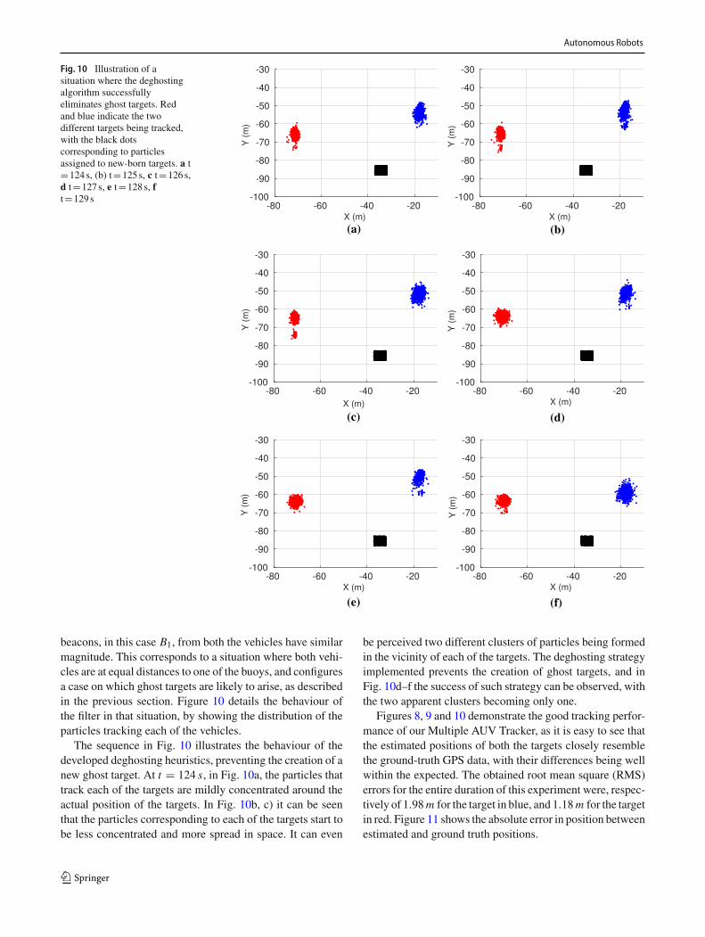
Fig. 10 Illustration of asituation where the deghostingalgorithm successfullyeliminates ghost targets. Redand blue indicate the twodifferent targets being tracked,with the black dotscorresponding to particlesassigned to new-born targets. a t=124s, (b) t=125s, c t=126s,d t=127s, e t=128s, ft=129s

(a) (b)

(c) (d)

(e) (f)

beacons, in this case B1, from both the vehicles have similarmagnitude. This corresponds to a situation where both vehi-cles are at equal distances to one of the buoys, and configuresa case on which ghost targets are likely to arise, as describedin the previous section. Figure 10 details the behaviour ofthe filter in that situation, by showing the distribution of theparticles tracking each of the vehicles.

The sequence in Fig. 10 illustrates the behaviour of thedeveloped deghosting heuristics, preventing the creation of anew ghost target. At t = 124 s, in Fig. 10a, the particles thattrack each of the targets are mildly concentrated around theactual position of the targets. In Fig. 10b, c) it can be seenthat the particles corresponding to each of the targets start tobe less concentrated and more spread in space. It can even

be perceived two different clusters of particles being formedin the vicinity of each of the targets. The deghosting strategyimplemented prevents the creation of ghost targets, and inFig. 10d–f the success of such strategy can be observed, withthe two apparent clusters becoming only one.

Figures 8, 9 and 10 demonstrate the good tracking perfor-mance of our Multiple AUV Tracker, as it is easy to see thatthe estimated positions of both the targets closely resemblethe ground-truth GPS data, with their differences being wellwithin the expected. The obtained root mean square (RMS)errors for the entire duration of this experiment were, respec-tively of 1.98m for the target in blue, and 1.18m for the targetin red. Figure 11 shows the absolute error in position betweenestimated and ground truth positions.

123

Autonomous Robots

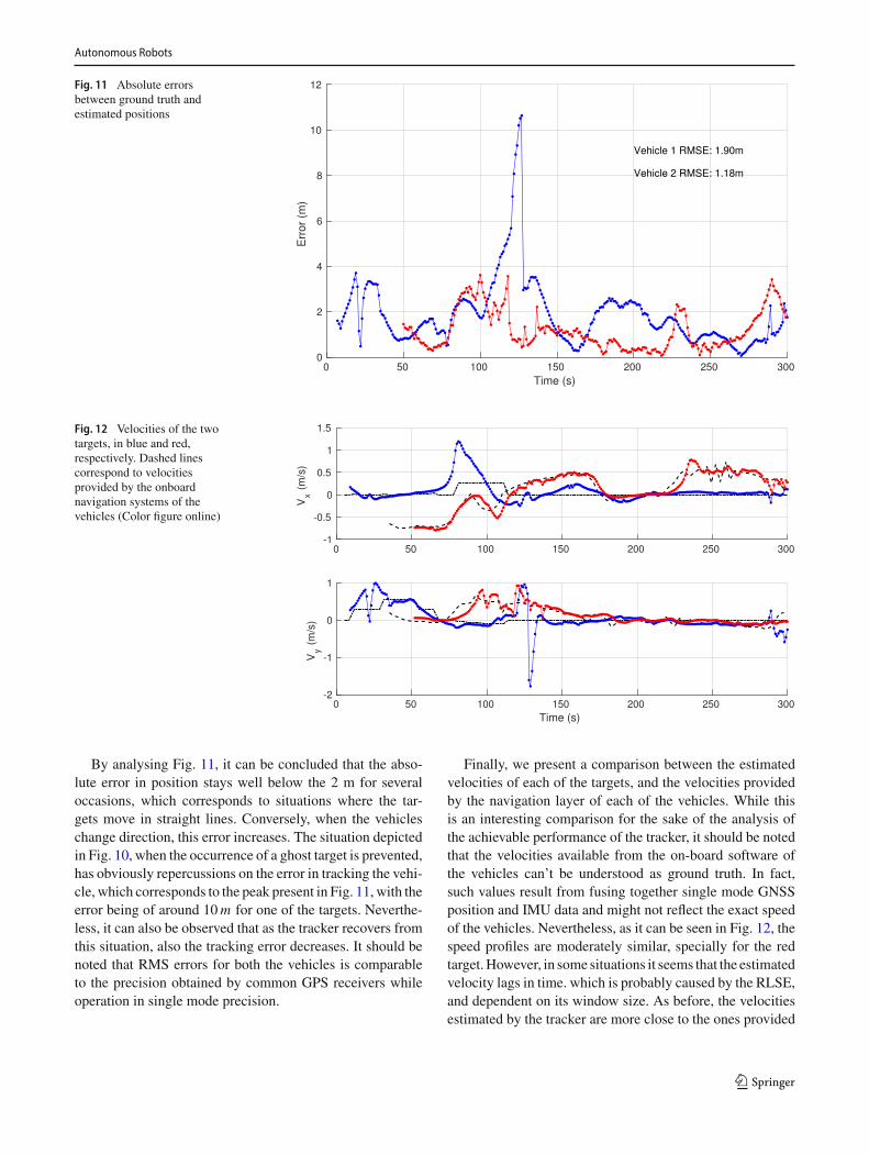
Fig. 11 Absolute errorsbetween ground truth andestimated positions

Fig. 12 Velocities of the twotargets, in blue and red,respectively. Dashed linescorrespond to velocitiesprovided by the onboardnavigation systems of thevehicles (Color figure online)

By analysing Fig. 11, it can be concluded that the abso-lute error in position stays well below the 2 m for severaloccasions, which corresponds to situations where the tar-gets move in straight lines. Conversely, when the vehicleschange direction, this error increases. The situation depictedin Fig. 10, when the occurrence of a ghost target is prevented,has obviously repercussions on the error in tracking the vehi-cle, which corresponds to the peak present in Fig. 11, with theerror being of around 10m for one of the targets. Neverthe-less, it can also be observed that as the tracker recovers fromthis situation, also the tracking error decreases. It should benoted that RMS errors for both the vehicles is comparableto the precision obtained by common GPS receivers whileoperation in single mode precision.

Finally, we present a comparison between the estimatedvelocities of each of the targets, and the velocities providedby the navigation layer of each of the vehicles. While thisis an interesting comparison for the sake of the analysis ofthe achievable performance of the tracker, it should be notedthat the velocities available from the on-board software ofthe vehicles can’t be understood as ground truth. In fact,such values result from fusing together single mode GNSSposition and IMU data and might not reflect the exact speedof the vehicles. Nevertheless, as it can be seen in Fig. 12, thespeed profiles are moderately similar, specially for the redtarget.However, in some situations it seems that the estimatedvelocity lags in time. which is probably caused by the RLSE,and dependent on its window size. As before, the velocitiesestimated by the tracker are more close to the ones provided

123

Autonomous Robots

by the navigation layer when the vehicles are moving in forstraight-line.

8 Conclusion

Operations with multiple vehicles are likely to become veryappealing in a near future, not only in terms of flexibility andefficiency, but also in termsof performing a set task that other-wise would not be possible. While the problem of providingnavigational aids to multiple vehicles has been addressedin the past, tracking multiple AUVs is a problem that hasbeen overlooked. In this article we presented an effectiveAUV Tracker for simultaneously tracking multiple vehicles,and successfully demonstrated its performance for real worldscenarios. Up to the authors knowledge, this is the first timethat a similar approach has been proposed and experimen-tally validated. Moreover, a similar strategy can be appliedto related applications, such as the localization and trackingof multiple underwater acoustic sources.

It was demonstrated that the problem of tracking of multi-ple AUVs can be successfully tackled using PHD filters. TheRFS nature of the PHD filter doesn’t require a specific asso-ciation between measurements and the targets that producedthem, thus making it appropriate for this problem. Also, withthis strategy there is no need to develop intricate solutions todistinguish vehicles, such as complex hardware for modulat-ing the acoustic signals. The tracking results achieved werevery positive, with RMS errors under 2 meters, which is ofsimilar precision towhat can be obtainedwith aGPS receiver.Moreover, the proposed filter is also able to keep informa-tion of the track continuity along the time. Such results wereobtained despite the quite adverse trajectories performed bythe vehicles, very close to each other, and with the vehi-cles moving with arbitrary low speeds. It should also beunderlined that such results have been achieved despite theunfavourable geometry of the acoustic network, with onlytwo beacons and with a baseline not very long.

While the results achieved are very encouraging, it can beargued that we addressed a situation with only two targets.While this is true, there is no indication that the developedtracker would have behaved differently with more targetsappearing and disappearing in the area under surveillance.While the computational complexity of the filter dependsexponentially on the number of clutter measurements, andthis numberwould obviously increasewith the number of tar-gets being tracked, the implementation of an adequate gatingstrategy, as it has been proposed elsewhere, is able to prop-erly deal with this issue. On the other hand, the processingtime of the algorithm, for the full duration of the scenarioin analysis, is well below the actual time, thus no real-timeperformance issues are likely to arise.

As a final remark, it should bementioned that even thoughthe proposed approached was focused on tracking AUVs,it’s applicability can be broader. As it was made clear inSect. 2, the topic of underwater target tracking is broader andencompasses more areas than just the underwater roboticscommunity. Therefore, it would be interesting to study theapplicability of the proposedmethod to other areas, for exam-ple related to underwater wireless sensor networks, or evensource localization problems.

Acknowledgements This work is financed by the ERDF—EuropeanRegional Development Fund through the Operational Programmefor Competitiveness and Internationalisation - COMPETE 2020 Pro-gramme, and by National Funds through the FCT—Fundação para aCiência e a Tecnologia (Portuguese Foundation for Science and Tech-nology) within project « POCI-01-0145-FEDER-006961 ». The firstauthor was supported by the Portuguese Foundation for Science andTechnology through the Ph.D. grant SFRH/BD/70727/2010.

Compliance with ethical standards

Conflicts of interest The authors declare that they have no conflict ofinterest.

References

Almeida, R., Melo, J., & Cruz, N. (2016). Characterization of measure-ment errors in a LBL positioning system. In Proceedings of theMTS/IEEE Oceans’16 Conference, Shanghai, China.

Bar-Shalom, Y., & Li, X. (1995). Multitarget-multisensor tracking:Principles and techniques. London: Yaakov Bar-Shalom.

Braca, P., Goldhahn, R., LePage, K., Marano, S., Matta, V., &Willett, P.(2014). Cognitive multistatic AUV networks. In 2014 17th inter-national conference on information fusion (FUSION) (pp. 1–7).

Choi, J. & Choi, H. -T. (2015). Multi-target localization of underwa-ter acoustic sources based on probabilistic estimation of directionangle. In Proceedings of the MTS/IEEE Oceans’15 conference,Genova, Italy (pp. 1–6).

Clark, D., & Bell, J. (2007). Multi-target state estimation and track con-tinuity for the particle phd filter. IEEE Transactions on Aerospaceand Electronic Systems, 43(4), 1441–1453.

Clark, D. E. (2006). Multiple target tracking with the probabilityhypothesis density filter. Ph.D. thesis, Heriot-Watt University.

Cruz, N., Matos, A., Cunha, S., & Silva, S. (2007). Zarco—Anautonomous craft for underwater surveys. In Proceedings of the7th geomatic week, Barcelona, Spain.

Erdinc, O., Willett, P., & Coraluppi, S. (2008). The gaussian mixturecardinalized phd tracker on mstwg and seabar datasets. In Infor-mation Fusion, 2008 11th International Conference on, pages 1–8.

Fiorelli, E., Leonard, N., Bhatta, P., Paley, D., Bachmayer, R., &Fratantoni, D. (2006). Multi-auv control and adaptive samplingin monterey bay. IEEE Journal of Oceanic Engineering, 31(4),935–948.

Fulton, T. F., Cassidy, C. J., Stokey, R. G., & Leonard, J. J. (2000).Navigation sensor data fusion for the AUV REMUS. In Proceed-ings of the symposium on underwater robotic technology, WorldAutomation Congress, Hawaii.

Georgescu, R., Schoenecker, S., & Willett, P. (2009). Gm-cphd andmlpda applied to the seabar07 and tno-blindmulti-static sonar data.

123

Autonomous Robots

In 2009. FUSION ’09. 12th international conference on informa-tion fusion (pp. 1851–1858).

Georgy, J., & Noureldin, A. (2014). Unconstrained underwater multi-target tracking in passive sonar systems using two-stage pf-basedtechnique. International Journal of Systems Science, 45(3), 439–455.

Georgy, J., Noureldin, A., & Mellema, G. (2012). Clustered mixtureparticle filter for underwater multitarget tracking in multistaticactive sonobuoy systems. IEEE Transactions on Systems, Man,and Cybernetics, Part C: Applications and Reviews, 42(4), 547–560.

Granstrom, K., Lundquist, C., Gustafsson, F., & Orguner, U. (2014).Random set methods: Estimation of multiple extended objects.IEEE Robotics and Automation Magazine, 21(2), 73–82.

Hol, J., Schon, T., & Gustafsson, F. (2006). On resampling algorithmsfor particle filters. In 2006 IEEE nonlinear statistical signal pro-cessing workshop (pp. 79–82).

Kreucher, C., & Shapo, B. (2011). Multitarget detection and trackingusing multisensor passive acoustic data. IEEE Journal of OceanicEngineering, 36(2), 205–218.

Lang, T., Dunne,D.,&Mellema,G. (2009). An assessment of hierarchi-cal data fusion using seabar’07 data. In 2009. FUSION ’09. 12thinternational conference on information fusion (pp. 1560–1567).

Leonard, N. E., Paley, D. A., Davis, R. E., Fratantoni, D. M., Lekien, F.,& Zhang, F. (2010). Coordinated control of an underwater gliderfleet in an adaptive ocean sampling field experiment in montereybay. Journal of Field Robotics, 27(6), 718–740.

Lin, L., Bar-Shalom, Y., & Kirubarajan, T. (2006). Track labeling andphdfilter formultitarget tracking. IEEE Transactions on Aerospaceand Electronic Systems, 42(3), 778–795.

Ma, W.-K., Vo, B.-N., Singh, S., & Baddeley, A. (2006). Tracking anunknown time-varying number of speakers using tdoa measure-ments: A random finite set approach. IEEE Transactions on SignalProcessing, 54(9), 3291–3304.

Mahler, R. (2003). Multitarget bayes filtering via first-order multitargetmoments. IEEE Transactions on Aerospace and Electronic Sys-tems, 39(4), 1152–1178.

Mahler, R. (2008). Random set theory formultisource-multitarget infor-mation fusion. In M. E. Liggins, D. L. Hall, & J. Llinas (Eds.),Handbook of multisensor data fusion: Theory and practice (sec-ond ed., pp. 369–410). Boca Raton: CRC Press.

Mahler, R. (2013). “statistics 102” formultisource-multitarget detectionand tracking. IEEE Journal of Selected Topics in Signal Process-ing, 7(3), 376–389.

Marino, A., Antonelli, G., Aguiar, A., Pascoal, A., & Chi-averini, S. (2015). A decentralized strategy for multirobot sam-pling/patrolling: Theory and experiments. IEEE Transactions onControl Systems Technology, 23(1), 313–322.

Matos, A., Cruz, N., Martins, A., & Pereira, F. (1999). Developmentand implementation of a low-cost lbl navigation system for an auv.In Proceedings of the MTS/IEEE Oceans’99 conference (Vol. 2,pp. 774–779). Seattle, USA.

Mazurek, P. (2008). Deghosting methods for track-before-detect mul-titarget multisensor algorithms. In J. M. R. Arreguin (Ed.),Automation and Robotics. I-Tech Education and Publishing.

Melo, J., & Matos, A. (2008). Guidance and control of an asv in auvtracking operations. In Proceedings of the MTS/IEEE Oceans’08conference (pp. 1–7), Quebec City, Canada.

Melo, J., & Matos, A. (2014). A phd filter for tracking multiple auvs.In Proceedings of the MTS/IEEE Oceans’14 conference (pp. 1–8),St. John’s, Canada.

Morelande, M., Suvorova, S., Fletcher, F., Simakov, S., & Moran, B.(2015). Multi-target tracking for multistatic sonobuoy systems.In 2015 18th International Conference on Information Fusion(Fusion) (pp. 327–332).

Napolitano, F., Cretollier, F., & Pelletier, H. (2005). Gaps, combinedusbl + ins +gps tracking system for fast deployable amp; high accu-racy multiple target positioning. In Proceedings of the MTS/IEEEOceans’08 conference (Vol. 2, pp. 1415–1420), Brest, France.

Odell, D., Hertel, K., & Nielsen, C. (2002). New acoustic systems forauv tracking, communications, and noise measurement at nswccd-ard, lake pend oreille, idaho. In Proceedings of the MTS/IEEEOceans’02 conference (Vol. 1, pp. 266–271), Biloxi, USA.

Paull, L., Huang, G., Seto, M., & Leonard, J. (2015). Communication-constrained multi-auv cooperative slam. In 2015 IEEE inter-national conference on robotics and automation (ICRA) (pp.509–516).

Peñas, A. A. (2009). Positioning and navigation systems for roboticunderwater vehicles. Ph.D. thesis, Instituto Superior Técnico, Uni-versidade Técnica de Lisboa.

Prins, R., & Kandemir, M. (2008). Time-constrained optimizationof multi-auv cooperative mine detection. In Proceedings ofthe MTS/IEEE Oceans’08 conference (pp. 1–13), Quebec City,Canada.

Schulz, B., Hobson, B., Kemp, M., Meyer, J., Moody, R., Pinnix, H.,& St Clair, M. (2003). Field results of multi-uuv missions usingranger micro-uuvs. In Proceedings of the MTS/IEEE Oceans’03conference (Vol. 2, pp. 956–961), San Diego, USA.

Stone, L., Streit, R., Corwin, T., & Bell, K. (2013). Bayesian multipletarget tracking, Second Edition: Radar/Remote Sensing. ArtechHouse.

Vahidi, A., Stefanopoulou, A., & Peng, H. (2005). Recursive leastsquares with forgetting for online estimation of vehicle mass androad grade: Theory and experiments. Vehicle System Dynamics,43(1), 31–55.

Vo, B. N., & Ma, W. K. (2005). A closed-form solution for the proba-bility hypothesis density filter. In 7th international conference oninformation fusion (Vol. 2, p. 8).

Vo, B.-N., Singh, S., & Doucet, A. (2005). Sequential monte carlomethods for multitarget filtering with random finite sets. IEEETransactions on Aerospace and Electronic Systems, 41(4), 1224–1245.

Vo, B.-T., & Vo, B.-N. (2013). Labeled random finite sets and multi-object conjugate priors. IEEE Transactions on Signal Processing,61(13), 3460–3475.

Wang, X., Xu, M., Wang, H., Wu, Y., & Shi, H. (2012). Combina-tion of interacting multiple models with the particle filter forthree-dimensional target tracking in underwater wireless sensornetworks. Mathematical Problems in Engineering, 2012(829451),1–16.

Watanabe, Y., Ochi, H., Shimura, T., & Hattori, T. (2009). A tracking ofauv with integration of ssbl acoustic positioning and transmittedins data. In Proceedings of the MTS/IEEE Oceans’09 conference(pp. 1–6), Bremen, Germany.

Yang, R., Ng, G. W., & Bar-Shalom, Y. (2013). Tracking/fusion anddeghosting with doppler frequency from two passive acoustic sen-sors. In 2013 16th international conference on information fusion(FUSION) (pp. 1784–1790).

Zhang, S., Chen, H., & Liu, M. (2014). Adaptive sensor scheduling fortarget tracking in underwater wireless sensor networks. In 2014international conference on mechatronics and control (ICMC) (pp.55–60).

123

Autonomous Robots

José Melo is a postdoc researcherat the Center for Robotics andAutonomous Systems ofINESCTEC, in Porto. In 2016 hereceived his Ph.D. in Electricaland Computer Engineering fromthe Faculty of Engineering, Uni-versity of Porto. In 2008 hereceived his M.Sc. degree in Elec-trical and Computer Engineering,with a major in Automation, fromthe same University. In betweendegrees, and until 2010, José hasworked as a Software Engineer,at CERN. José is with the Ocean

Systems Group since 2010, when he started his Ph.D., and withINESCTEC since 2011, when he joined the Robotics and IntelligentSystems unit as a researcher. In 2015 he was an invited researcher atthe National Insitute of Informatics, Tokyo, Japan under the supervi-sion of Prof. Kenki Tei, in Honiden Lab. His current research interestsare in the area of Navigation and Sensor Fusion for Autonomous Vehi-cles.

Aníbal C.Matos received the Ph.D.degree in Electrical and ComputerEngineering from the Universityof Porto, Porto, Portugal, in 2001.Currently, he coordinates de Cen-tre for Robotics and AutonomousSystems at INESC TEC and holdsan assistant professor position atthe Faculty of Engineering of theUniversity of Porto. His mainresearch interests are related tonavigation and control ofautonomous underwater and sur-face vehicles. He has been and iscurrently involved in several R&D

projects related to the development and applications of marine vehi-cles, funded by several national and international agencies.

123