Designing Practical Motions for AutonomousUnderwater Vehicles: A Ship Hull Survey Mission

R.N. Smith∗,1

Robotic Embedded Systems Laboratory, Department of Computer Science,University of Southern California, Los Angeles, CA 90089, USA

M. Chyba, S.B. Singh1

Mathematics Department, College of Natural Sciences,University of Hawai‘i, Honolulu, HI 96822, USA

S.K. Choi, G. Marani2

Autonomous Systems Laboratory, College of Engineering,University of Hawai‘i, Honolulu, HI 96822, USA

Abstract

The primary focus of this paper is to provide a solution to thepractical motion planningproblem of a ship hull survey to be performed by an AutonomousUnderwater Vehicle(AUV). In particular, we examine the bulbous bow portion of the hull and present a reason-able survey strategy. Unique to this applied study, is the approach to the problem via differ-ential geometric techniques. The motion planning problem is solved by use of a geometricreduction to the dynamic equations of motion, and the trajectory is generated through theconcatenation of kinematic motions. The control strategy for each arc of the trajectory iscalculated and implemented onto a test-bed vehicle. Experimental results are presented todemonstrate the effectiveness of this motion planning solution.

Key words: Applied Motion Planning, Kinematic Motion, Autonomous UnderwaterVehicle, Experimental Validation, Ship Hull Survey, Bulbous Bow

∗ Corresponding author.Email address:ryannsmi@usc.edu (R.N. Smith).

1 This research is supported in part by the National Science Foundation grant DMS-06085832 This research is supported in part by the Office of Naval Research grants N00014-03-1-0969, N00014-04-1-0751 and N00014-04-1-0751

Preprint submitted to Elsevier 6 April 2009

1 Introduction

Approximately 90% of the goods traded throughout the world are carried by theinternational shipping industry. What many consider to be anormal life, wouldnot be possible without maritime shipping. With incentivesof competitive freightcosts during a time of increasing fuel expenses, seaborne trade continues to ex-pand. Thus, prospects for the maritime industry’s further growth continues to bestrong. Currently, there are more than 50,000 merchant ships trading internation-ally and transporting may different types of cargo. This fleet belongs to more than150 nations, and employs over a million seafarers.

With a high volume of ships arriving from worldwide destinations, it is of utmostimportance to monitor and protect the ports which are so crucial to a country’strading market. To this end, it has become an interest of homeland security andport authorities to examine the hulls of ships before they enter port. This problemhas attracted much research interest in the Autonomous Underwater Vehicle (AUV)and ocean engineering community and is currently still under much investigation.We do not propose to entirely solve the matter here, but offera solution to a motionplanning problem motivated from ship hull inspections.

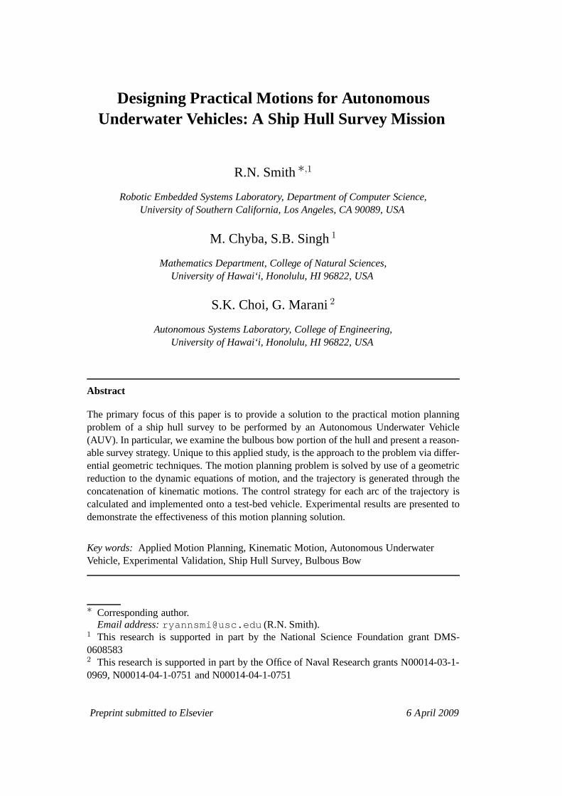
Fig. 1. USS George H.W. Bush (CVN77), GlobalSecurity.org (2008).

Many of the large vessels which would re-quire examination before entering a porthave a bulbous bow. An example of suchcan be seen on the USS George H.W. Bush(CVN 77) shown in Fig. 1. This bulb ispositioned to sit just below the design wa-ter line and has the purpose of reducingthe height of the bow wake of the vesselwhich in turn reduces the hull drag whichimplies better efficiency. Bulbs come inall different shapes and sizes and are op-timized for a given ship design. Such afeature provides an interesting control the-ory problem for which to consider motionplanning and trajectory design.

In this paper, we approach the motion planning problem and control strategy designby use of the architecture of differential geometry. This framework provides thestructure necessary to consider an agile AUV that can move inall six degrees-of-freedom (DOF). Additionally, this framework includes a straightforward methodto accommodate under-actuated scenarios, such as thrusterfailure or consideringa standard torpedo-shaped vehicle. Recent research has shown that such geometricmethods can be used to design implementable control strategies for AUVs, and isan effective method for solving the motion planning problem, c.f., Smith (2008).

2

We begin by developing the equations of motion for the submerged rigid body ina traditional manner, followed by the same equations presented in the languageof differential geometry. We include a short section to motivate the use of thisgeometric architecture and give a literature review of similar research. Section 4describes the design and calculation of the control strategies and includes the ac-tual controls to be implemented onto a test-bed vehicle. Theimplementation ofthe calculated control strategies are carried out on the Omni-Directional IntelligentNavigator (ODIN), which is owned and maintained by the Autonomous SystemsLaboratory, College of Engineering, University of Hawaii.Experimental resultsfrom these tests are presented in Section 5, which also includes analysis of theseimplementations. We conclude this paper with an overall assessment and provideideas for future research.

2 Equations of Motion

In this section, we present a working model for the kinematics and dynamics of asubmerged, three-dimensional rigid body that can move in six degrees-of-freedom.These equations assume that the body is submerged in a viscous fluid and incor-porate the forces and moments arising from added mass, hydrodynamic damping,gravity and buoyancy.

A derivation of the general rigid body equations of motion can be found in a clas-sical mechanics text such as Lamb (1961), Meriam and Kraige (1997) or Ardema(2005). The addition of the hydrodynamic forces and momentsinto these generalequations can be found in Lamb (1945) (see also Fossen, 1994), with an in-depthtreatment of the hydrodynamic topics presented in Newman (1977).

In the sequel, we will use methods from geometric control theory to design thecontrol strategies to be implemented onto the test-bed vehicle. To this end, we con-sider the equations of motion for the submerged rigid body expressed by use of thelanguage of differential geometry. Since a derivation of these geometric equationswould require an extensive background of language and notation which is beyondthe scope of this paper, we refer the reader to Smith (2008) for a detailed derivationof both the classical equations and those derived by use of the geometric controlframework.

2.1 Preliminary Kinematics

For the analysis of AUVs, it is necessary to work with two right-handed, orthog-onal coordinate systems. We first need a reference frame fromwhich to measuredistances and angles. This is done by choosing an earth-fixedreference frame. Forlow-speed marine vehicles such as those studied here, the Earth’s movement has anegligible effect on the dynamics of the vehicle. Thus, the earth-fixed frame maybe considered as an inertial frame. To precisely identify the configuration of a rigidbody, we need to know the position and orientation of a point on the body with

3

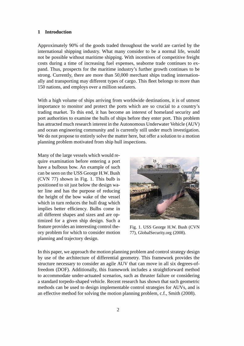
respect to the inertial reference frame. Thus, we will definea reference frame fixedto a chosen point on the body. These two reference frames are described in detailbelow.

Fig. 2. Earth-fixed and body-fixed coordinatereference frames.

The inertial frame is a right-handed,non-rotating, orthogonal referenceframe and is taken to be earthfixed with accelerations neglected.This coordinate systemΣI : (OI ,

s1, s2, s3) is defined with thes1

and s2 axes lying in the horizontalplane perpendicular to the directionof gravity, while thes3 axis is or-thogonal to thes1 − s2 plane andtaken to be positive in the direc-tion of gravity. We may also referto this frame as the spatial referenceframe. This choice of inertial refer-ence frame is consistent with currentoceanography and AUV literature.With this choice of coordinates, weget a reference frame positioned atthe free surface(s3 = 0) ands3 corresponds to depth. Since we are consideringan unbounded fluid domain, we may select an arbitrary position for the inertialframe, preferably in a location such that the depth of the vehicle is non-negative.The inertial frame is shown in Fig. 2.

The body-fixed frame, shown in Fig. 2, is a right-handed, orthogonal referenceframe which is fixed to a point on the body. This coordinate systemΣB : (OB, B1,

B2, B3) is defined withOB located at a chosen point and the body axesB1, B2

andB3 coincide with the principle axes of inertia:

• B1 - longitudinal axis (positive to fore)• B2 - transverse axis (positive to starboard)• B3 - normal axis (positive to the keel)

The above definitions of reference frames suggests that the position and orientationof the vehicle be expressed relative to the spatial frame while the linear and angularvelocities are defined relative to the body-fixed frame. Standard notation for thesequantities are defined in SNAME (1950) and are reproduced in Table 1.

As seen in Fig. 2, we letb = (x, y, z) be the vector from the origin of the in-ertial frame to the origin of the body-fixed frame. The angular orientation of thebody with respect to the earth-fixed frame can either be givenusing Euler angles orquaternions. In this dissertation, we choose to work with the Euler angles, accepting

4

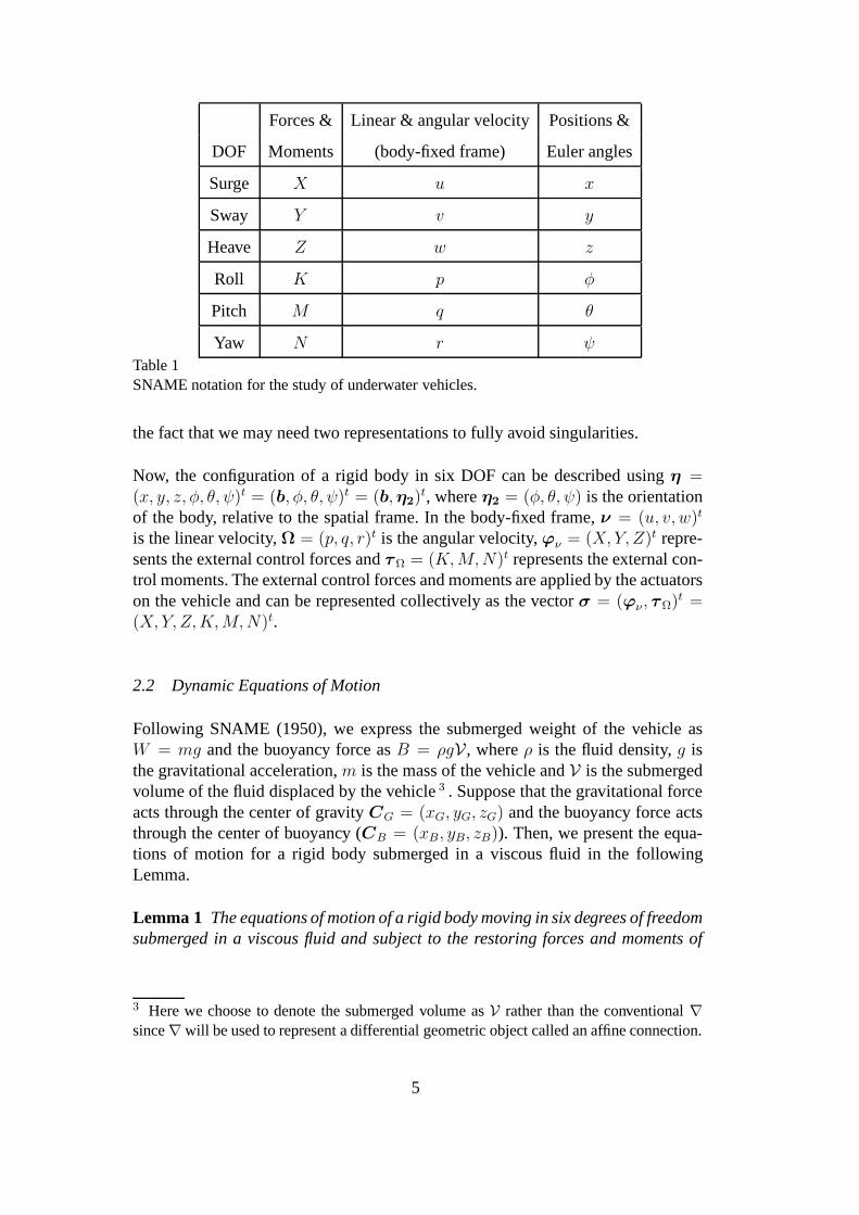
Forces & Linear & angular velocity Positions &

DOF Moments (body-fixed frame) Euler angles

Surge X u x

Sway Y v y

Heave Z w z

Roll K p φ

Pitch M q θ

Yaw N r ψ

Table 1SNAME notation for the study of underwater vehicles.

the fact that we may need two representations to fully avoid singularities.

Now, the configuration of a rigid body in six DOF can be described usingη =(x, y, z, φ, θ, ψ)t = (b, φ, θ, ψ)t = (b,η2)

t, whereη2 = (φ, θ, ψ) is the orientationof the body, relative to the spatial frame. In the body-fixed frame,ν = (u, v, w)t

is the linear velocity,Ω = (p, q, r)t is the angular velocity,ϕν = (X, Y, Z)t repre-sents the external control forces andτΩ = (K,M,N)t represents the external con-trol moments. The external control forces and moments are applied by the actuatorson the vehicle and can be represented collectively as the vector σ = (ϕν , τΩ)t =(X, Y, Z,K,M,N)t.

2.2 Dynamic Equations of Motion

Following SNAME (1950), we express the submerged weight of the vehicle asW = mg and the buoyancy force asB = ρgV, whereρ is the fluid density,g isthe gravitational acceleration,m is the mass of the vehicle andV is the submergedvolume of the fluid displaced by the vehicle3 . Suppose that the gravitational forceacts through the center of gravityCG = (xG, yG, zG) and the buoyancy force actsthrough the center of buoyancy (CB = (xB, yB, zB)). Then, we present the equa-tions of motion for a rigid body submerged in a viscous fluid inthe followingLemma.

Lemma 1 The equations of motion of a rigid body moving in six degrees of freedomsubmerged in a viscous fluid and subject to the restoring forces and moments of

3 Here we choose to denote the submerged volume asV rather than the conventional∇since∇ will be used to represent a differential geometric object called an affine connection.

5

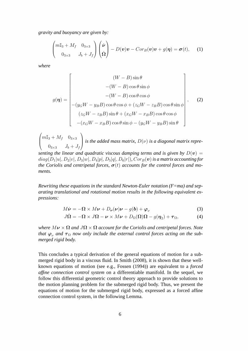
gravity and buoyancy are given by:

mI3 +Mf 03×3

03×3 Jb + Jf

ν

Ω

−D(v)v − CorB(v)v + g(η) = σ(t), (1)

where

g(η) =

(W − B) sin θ

−(W − B) cos θ sinφ

−(W − B) cos θ cosφ

−(yGW − yBB) cos θ cosφ+ (zGW − zBB) cos θ sin φ

(zGW − zBB) sin θ + (xGW − xBB) cos θ cosφ

−(xGW − xBB) cos θ sinφ− (yGW − yBB) sin θ

, (2)

mI3 +Mf 03×3

03×3 Jb + Jf

is the added mass matrix,D(ν) is a diagonal matrix repre-

senting the linear and quadratic viscous damping terms and is given byD(v) =diag(D1|u|, D2|v|, D3|w|, D4|p|, D5|q|, D6|r|),CorB(v) is a matrix accounting forthe Coriolis and centripetal forces,σ(t) accounts for the control forces and mo-ments.

Rewriting these equations in the standard Newton-Euler notation (F=ma) and sep-arating translational and rotational motion results in thefollowing equivalent ex-pressions:

M ν = −Ω ×Mν +Dν(ν)ν − g(b) + ϕν (3)

JΩ = −Ω × JΩ − ν ×Mν +DΩ(Ω)Ω − g(η2) + τΩ, (4)

whereMν ×Ω andJΩ×Ω account for the Coriolis and centripetal forces. Notethat ϕν and τΩ now only include the external control forces acting on the sub-merged rigid body.

This concludes a typical derivation of the general equations of motion for a sub-merged rigid body in a viscous fluid. In Smith (2008), it is shown that these well-known equations of motion (see e.g., Fossen (1994)) are equivalent to aforcedaffine connection control systemon a differentiable manifold. In the sequel, wefollow this differential geometric control theory approach to provide solutions tothe motion planning problem for the submerged rigid body. Thus, we present theequations of motion for the submerged rigid body, expressedas a forced affineconnection control system, in the following Lemma.

6

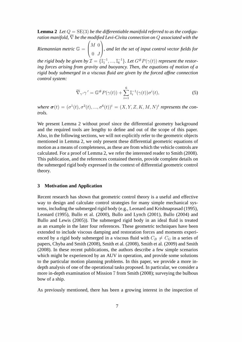
Lemma 2 LetQ = SE(3) be the differentiable manifold referred to as the configu-ration manifold,∇ be the modified Levi-Civita connection onQ associated with the

Riemannian metricG =

M 0

0 J

, and let the set of input control vector fields for

the rigid body be given byI = I−11 , ..., I−1

6 . LetG#P (γ(t)) represent the restor-ing forces arising from gravity and buoyancy. Then, the equations of motion of arigid body submerged in a viscous fluid are given by the forcedaffine connectioncontrol system:

∇γ ′γ ′ = G#P (γ(t)) +

6∑

i=1

I−1i (γ(t))σi(t), (5)

whereσ(t) = (σ1(t), σ2(t), ..., σ6(t))t = (X, Y, Z,K,M,N)t represents the con-trols.

We present Lemma 2 without proof since the differential geometry backgroundand the required tools are lengthy to define and out of the scope of this paper.Also, in the following sections, we will not explicitly refer to the geometric objectsmentioned in Lemma 2, we only present these differential geometric equations ofmotion as a means of completeness, as these are from which thevehicle controls arecalculated. For a proof of Lemma 2, we refer the interested reader to Smith (2008).This publication, and the references contained therein, provide complete details onthe submerged rigid body expressed in the context of differential geometric controltheory.

3 Motivation and Application

Recent research has shown that geometric control theory is auseful and effectiveway to design and calculate control strategies for many simple mechanical sys-tems, including the submerged rigid body (e.g., Leonard andKrishnaprasad (1995),Leonard (1995), Bullo et al. (2000), Bullo and Lynch (2001),Bullo (2004) andBullo and Lewis (2005)). The submerged rigid body in an idealfluid is treatedas an example in the later four references. These geometric techniques have beenextended to include viscous damping and restoration forcesand moments experi-enced by a rigid body submerged in a viscous fluid withCB 6= CG in a series ofpapers, Chyba and Smith (2008), Smith et al. (2008), Smith etal. (2009) and Smith(2008). In these recent publications, the authors describea few simple scenarioswhich might be experienced by an AUV in operation, and provide some solutionsto the particular motion planning problems. In this paper, we provide a more in-depth analysis of one of the operational tasks proposed. In particular, we consider amore in-depth examination of Mission7 from Smith (2008); surveying the bulbousbow of a ship.

As previously mentioned, there has been a growing interest in the inspection of

7

ship hulls as well as port facilities. These tasks are physically intensive and requirethe involvement of highly-skilled human divers. Such laborintensive work comeswith a potential risk to the diver. These risks are exponentially increased in thecase when hazardous foreign elements, such as explosives, are present. In an effortto reduce the risk to human life, the use of Remotely OperatedVehicles (ROVs)are being called upon for this task. However, this procedurealso requires intensehuman involvement for safely piloting the vehicle around the ship. Moreover, bothof these methods do not guarantee100% coverage, as the area around a ship inberth can be highly confined and cluttered. Operation of a tethered vehicle in theseconfines makes it even more difficult to perform the task successfully.

Due to ever pressing military reasons, engineers have been working on automatingthis process. By use of an AUV, we can reduce the risk to human life and addition-ally provide around-the-clock surveillance of ships and port facilities. With this asmotivation, we propose to apply geometric control theory todesign implementabletrajectories which control an AUV on a path to survey a portion of the hull or harborstructure.

Our choice of surveying the bulbous bow provides an interesting practical problemin many ways. First, due to its peculiar shape it is a challenging control problemfrom a geometrical point of view. Secondly, in rough water the body of the bulbis subjected to an alternating inflow velocity field, preventing the development ofstable destructive wave interference. Based on this type, as well as others typesof hydrodynamic forces faced by the bulb, it is imperative totake added care inits inspection and maintenance. Additionally, the problemof ship-dock structuredamage has existed since the primitive docks were constructed. Large ships havingbulbous bows are an added factor for such structure damage. Hence, we consider itimperative to have the ability to effectively survey the bulbous bow.

Since the shape of the bulb affects the performance of the vessel at sea, each bulbis uniquely constructed for an individual ship and many different shapes and sizescan be seen in use today. However, from a designers point of view, the bulb canessentially be approximated by a cylindrical solid capped with a hemisphere. This isthe simplified scenario that we assume for our experiments. Small alterations in theshape of the bulb will not greatly affect the design of our trajectories. Additionally,for very unique bulb shapes, similar methods to those described in the sequel canbe used to design trajectories which better fit those protrusions. Figure 3 displays atypical bulbous bow along with its dimensions.

4 Control Strategy

The control strategy presented here was designed by following the procedure out-lined in Chapter4 of Smith (2008), and then adapting it for implementation ontothe considered test-bed vehicle as described in Chapter5 of the same reference. Tosummarize this procedure, we begin by first applying a geometric reduction pro-

8

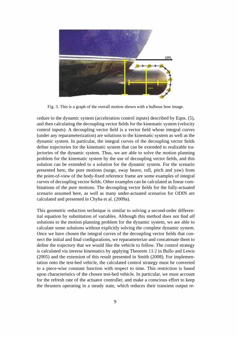
Fig. 3. This is a graph of the overall motion shown with a bulbous bow image.

cedure to the dynamic system (acceleration control inputs)described by Eqns. (5),and then calculating the decoupling vector fields for the kinematic system (velocitycontrol inputs). A decoupling vector field is a vector field whose integral curves(under any reparameterization) are solutions to the kinematic system as well as thedynamic system. In particular, the integral curves of the decoupling vector fieldsdefine trajectories for the kinematic system that can be extended to realizable tra-jectories of the dynamic system. Thus, we are able to solve the motion planningproblem for the kinematic system by the use of decoupling vector fields, and thissolution can be extended to a solution for the dynamic system. For the scenariopresented here, the pure motions (surge, sway heave, roll, pitch and yaw) fromthe point-of-view of the body-fixed reference frame are someexamples of integralcurves of decoupling vector fields. Other examples can be calculated as linear com-binations of the pure motions. The decoupling vector fields for the fully-actuatedscenario assumed here, as well as many under-actuated scenarios for ODIN arecalculated and presented in Chyba et al. (2009a).

This geometric reduction technique is similar to solving a second-order differen-tial equation by substitution of variables. Although this method does not findallsolutions to the motion planning problem for the dynamic system, we are able tocalculate some solutions without explicitly solving the complete dynamic system.Once we have chosen the integral curves of the decoupling vector fields that con-nect the initial and final configurations, we reparameterizeand concatenate them todefine the trajectory that we would like the vehicle to follow. The control strategyis calculated via inverse kinematics by applying Theorem13.2 in Bullo and Lewis(2005) and the extension of this result presented in Smith (2008). For implemen-tation onto the test-bed vehicle, the calculated control strategy must be convertedto a piece-wise constant function with respect to time. Thisrestriction is basedupon characteristics of the chosen test-bed vehicle. In particular, we must accountfor the refresh rate of the actuator controller, and make a conscious effort to keepthe thrusters operating in a steady state, which reduces their transient output re-

9

sponse. Since we are implementing in full open-loop, we try to reduce potentialerrors wherever possible. In the sequel, we present the calculated control strategiesin the piece-wise constant structure, since the focus of this paper is driven by theimplementation results and not the specific control design.

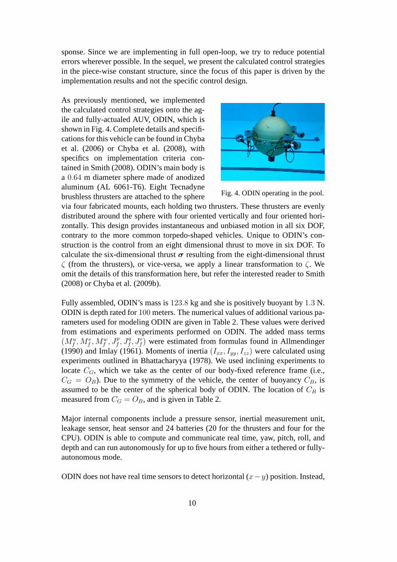
Fig. 4. ODIN operating in the pool.

As previously mentioned, we implementedthe calculated control strategies onto the ag-ile and fully-actualed AUV, ODIN, which isshown in Fig. 4. Complete details and specifi-cations for this vehicle can be found in Chybaet al. (2006) or Chyba et al. (2008), withspecifics on implementation criteria con-tained in Smith (2008). ODIN’s main body isa 0.64 m diameter sphere made of anodizedaluminum (AL 6061-T6). Eight Tecnadynebrushless thrusters are attached to the spherevia four fabricated mounts, each holding two thrusters. These thrusters are evenlydistributed around the sphere with four oriented vertically and four oriented hori-zontally. This design provides instantaneous and unbiasedmotion in all six DOF,contrary to the more common torpedo-shaped vehicles. Unique to ODIN’s con-struction is the control from an eight dimensional thrust tomove in six DOF. Tocalculate the six-dimensional thrustσ resulting from the eight-dimensional thrustζ (from the thrusters), or vice-versa, we apply a linear transformation toζ . Weomit the details of this transformation here, but refer the interested reader to Smith(2008) or Chyba et al. (2009b).

Fully assembled, ODIN’s mass is123.8 kg and she is positively buoyant by1.3 N.ODIN is depth rated for100 meters. The numerical values of additional various pa-rameters used for modeling ODIN are given in Table 2. These values were derivedfrom estimations and experiments performed on ODIN. The added mass terms(Mu

f ,Mvf ,M

wf , J

pf , J

qf , J

rf ) were estimated from formulas found in Allmendinger

(1990) and Imlay (1961). Moments of inertia(Ixx, Iyy, Izz) were calculated usingexperiments outlined in Bhattacharyya (1978). We used inclining experiments tolocateCG, which we take as the center of our body-fixed reference frame(i.e.,CG = OB). Due to the symmetry of the vehicle, the center of buoyancyCB, isassumed to be the center of the spherical body of ODIN. The location ofCB ismeasured fromCG = OB, and is given in Table 2.

Major internal components include a pressure sensor, inertial measurement unit,leakage sensor, heat sensor and 24 batteries (20 for the thrusters and four for theCPU). ODIN is able to compute and communicate real time, yaw,pitch, roll, anddepth and can run autonomously for up to five hours from eithera tethered or fully-autonomous mode.

ODIN does not have real time sensors to detect horizontal (x−y) position. Instead,

10

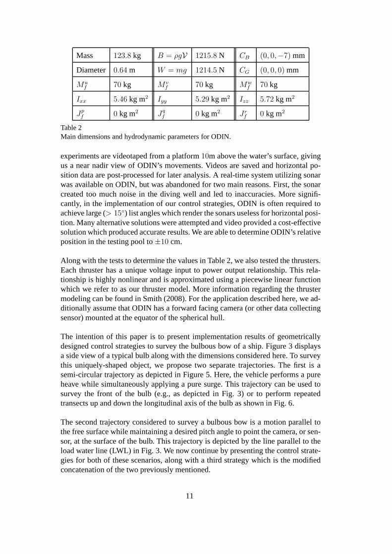
Mass 123.8 kg B = ρgV 1215.8 N CB (0, 0,−7) mm

Diameter 0.64 m W = mg 1214.5 N CG (0, 0, 0) mm

Muf 70 kg Mv

f 70 kg Mwf 70 kg

Ixx 5.46 kg m2 Iyy 5.29 kg m2 Izz 5.72 kg m2

Jpf 0 kg m2 J

qf 0 kg m2 Jr

f 0 kg m2

Table 2Main dimensions and hydrodynamic parameters for ODIN.

experiments are videotaped from a platform10m above the water’s surface, givingus a near nadir view of ODIN’s movements. Videos are saved andhorizontal po-sition data are post-processed for later analysis. A real-time system utilizing sonarwas available on ODIN, but was abandoned for two main reasons. First, the sonarcreated too much noise in the diving well and led to inaccuracies. More signifi-cantly, in the implementation of our control strategies, ODIN is often required toachieve large (> 15) list angles which render the sonars useless for horizontalposi-tion. Many alternative solutions were attempted and video provided a cost-effectivesolution which produced accurate results. We are able to determine ODIN’s relativeposition in the testing pool to±10 cm.

Along with the tests to determine the values in Table 2, we also tested the thrusters.Each thruster has a unique voltage input to power output relationship. This rela-tionship is highly nonlinear and is approximated using a piecewise linear functionwhich we refer to as our thruster model. More information regarding the thrustermodeling can be found in Smith (2008). For the application described here, we ad-ditionally assume that ODIN has a forward facing camera (or other data collectingsensor) mounted at the equator of the spherical hull.

The intention of this paper is to present implementation results of geometricallydesigned control strategies to survey the bulbous bow of a ship. Figure 3 displaysa side view of a typical bulb along with the dimensions considered here. To surveythis uniquely-shaped object, we propose two separate trajectories. The first is asemi-circular trajectory as depicted in Figure 5. Here, thevehicle performs a pureheave while simultaneously applying a pure surge. This trajectory can be used tosurvey the front of the bulb (e.g., as depicted in Fig. 3) or toperform repeatedtransects up and down the longitudinal axis of the bulb as shown in Fig. 6.

The second trajectory considered to survey a bulbous bow is amotion parallel tothe free surface while maintaining a desired pitch angle to point the camera, or sen-sor, at the surface of the bulb. This trajectory is depicted by the line parallel to theload water line (LWL) in Fig. 3. We now continue by presentingthe control strate-gies for both of these scenarios, along with a third strategywhich is the modifiedconcatenation of the two previously mentioned.

11

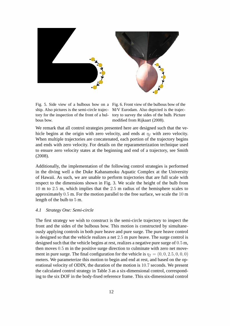
Fig. 5. Side view of a bulbous bow on aship. Also pictures is the semi-circle trajec-tory for the inspection of the front of a bul-bous bow.

Fig. 6. Front view of the bulbous bow of theM/V Eurodam. Also depicted is the trajec-tory to survey the sides of the bulb. Picturemodified from Rijkaart (2008).

We remark that all control strategies presented here are designed such that the ve-hicle begins at the origin with zero velocity, and ends atηf with zero velocity.When multiple trajectories are concatenated, each portionof the trajectory beginsand ends with zero velocity. For details on the reparameterization technique usedto ensure zero velocity states at the beginning and end of a trajectory, see Smith(2008).

Additionally, the implementation of the following controlstrategies is performedin the diving well a the Duke Kahanamoku Aquatic Complex at the Universityof Hawaii. As such, we are unable to perform trajectories that are full scale withrespect to the dimensions shown in Fig. 3. We scale the heightof the bulb from10 m to 2.5 m, which implies that the2.5 m radius of the hemisphere scales toapproximately0.5 m. For the motion parallel to the free surface, we scale the10 mlength of the bulb to5 m.

4.1 Strategy One: Semi-circle

The first strategy we wish to construct is the semi-circle trajectory to inspect thefront and the sides of the bulbous bow. This motion is constructed by simultane-ously applying controls in both pure heave and pure surge. The pure heave controlis designed so that the vehicle realizes a net2.5 m pure heave. The surge control isdesigned such that the vehicle begins at rest, realizes a negative pure surge of0.5 m,then moves0.5 m in the positive surge direction to culminate with zero net move-ment in pure surge. The final configuration for the vehicle isηf = (0, 0, 2.5, 0, 0, 0)meters. We parameterize this motion to begin and end at rest,and based on the op-erational velocity of ODIN, the duration of the motion is10.7 seconds. We presentthe calculated control strategy in Table 3 as a six-dimensional control, correspond-ing to the six DOF in the body-fixed reference frame. This six-dimensional control

12

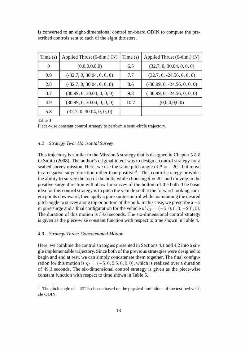
is converted to an eight-dimensional control on-board ODINto compute the pre-scribed controls sent to each of the eight thrusters.

Time (s) Applied Thrust (6-dim.) (N) Time (s) Applied Thrust (6-dim.) (N)

0 (0,0,0,0,0,0) 6.5 (32.7, 0, 30.04, 0, 0, 0)

0.9 (-32.7, 0, 30.04, 0, 0, 0) 7.7 (32.7, 0, -24.56, 0, 0, 0)

2.8 (-32.7, 0, 30.04, 0, 0, 0) 8.6 (-30.99, 0, -24.56, 0, 0, 0)

3.7 (30.99, 0, 30.04, 0, 0, 0) 9.8 (-30.99, 0, -24.56, 0, 0, 0)

4.9 (30.99, 0, 30.04, 0, 0, 0) 10.7 (0,0,0,0,0,0)

5.8 (32.7, 0, 30.04, 0, 0, 0)

Table 3Piece-wise constant control strategy to perform a semi-circle trajectory.

4.2 Strategy Two: Horizontal Survey

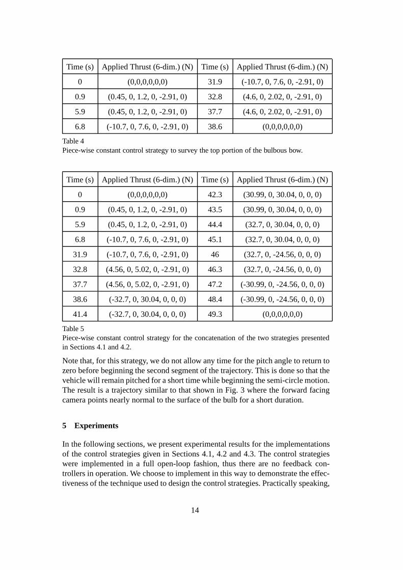
This trajectory is similar to the Mission5 strategy that is designed in Chapter5.5.5in Smith (2008). The author’s original intent was to design acontrol strategy for aseabed survey mission. Here, we use the same pitch angle ofθ = −20, but movein a negative surge direction rather than positive4 . This control strategy providesthe ability to survey the top of the bulb, while choosingθ = 20 and moving in thepositive surge direction will allow for survey of the bottomof the bulb. The basicidea for this control strategy is to pitch the vehicle so thatthe forward-looking cam-era points downward, then apply a pure surge control while maintaining the desiredpitch angle to survey along top or bottom of the bulb. In this case, we prescribe a−5m pure surge and a final configuration for the vehicle ofηf = (−5, 0, 0, 0,−20, 0).The duration of this motion is38.6 seconds. The six-dimensional control strategyis given as the piece-wise constant function with respect totime shown in Table 4.

4.3 Strategy Three: Concatenated Motion

Here, we combine the control strategies presented in Sections 4.1 and 4.2 into a sin-gle implementable trajectory. Since both of the previous strategies were designed tobegin and end at rest, we can simply concatenate them together. The final configu-ration for this motion isηf = (−5, 0, 2.5, 0, 0, 0), which is realized over a durationof 49.3 seconds. The six-dimensional control strategy is given as the piece-wiseconstant function with respect to time shown in Table 5.

4 The pitch angle of−20 is chosen based on the physical limitations of the test-bed vehi-

cle ODIN.

13

Time (s) Applied Thrust (6-dim.) (N) Time (s) Applied Thrust (6-dim.) (N)

0 (0,0,0,0,0,0) 31.9 (-10.7, 0, 7.6, 0, -2.91, 0)

0.9 (0.45, 0, 1.2, 0, -2.91, 0) 32.8 (4.6, 0, 2.02, 0, -2.91, 0)

5.9 (0.45, 0, 1.2, 0, -2.91, 0) 37.7 (4.6, 0, 2.02, 0, -2.91, 0)

6.8 (-10.7, 0, 7.6, 0, -2.91, 0) 38.6 (0,0,0,0,0,0)

Table 4Piece-wise constant control strategy to survey the top portion of the bulbous bow.

Time (s) Applied Thrust (6-dim.) (N) Time (s) Applied Thrust (6-dim.) (N)

0 (0,0,0,0,0,0) 42.3 (30.99, 0, 30.04, 0, 0, 0)

0.9 (0.45, 0, 1.2, 0, -2.91, 0) 43.5 (30.99, 0, 30.04, 0, 0, 0)

5.9 (0.45, 0, 1.2, 0, -2.91, 0) 44.4 (32.7, 0, 30.04, 0, 0, 0)

6.8 (-10.7, 0, 7.6, 0, -2.91, 0) 45.1 (32.7, 0, 30.04, 0, 0, 0)

31.9 (-10.7, 0, 7.6, 0, -2.91, 0) 46 (32.7, 0, -24.56, 0, 0, 0)

32.8 (4.56, 0, 5.02, 0, -2.91, 0) 46.3 (32.7, 0, -24.56, 0, 0, 0)

37.7 (4.56, 0, 5.02, 0, -2.91, 0) 47.2 (-30.99, 0, -24.56, 0, 0, 0)

38.6 (-32.7, 0, 30.04, 0, 0, 0) 48.4 (-30.99, 0, -24.56, 0, 0, 0)

41.4 (-32.7, 0, 30.04, 0, 0, 0) 49.3 (0,0,0,0,0,0)

Table 5Piece-wise constant control strategy for the concatenation of the two strategies presentedin Sections 4.1 and 4.2.

Note that, for this strategy, we do not allow any time for the pitch angle to return tozero before beginning the second segment of the trajectory.This is done so that thevehicle will remain pitched for a short time while beginningthe semi-circle motion.The result is a trajectory similar to that shown in Fig. 3 where the forward facingcamera points nearly normal to the surface of the bulb for a short duration.

5 Experiments

In the following sections, we present experimental resultsfor the implementationsof the control strategies given in Sections 4.1, 4.2 and 4.3.The control strategieswere implemented in a full open-loop fashion, thus there areno feedback con-trollers in operation. We choose to implement in this way to demonstrate the effec-tiveness of the technique used to design the control strategies. Practically speaking,

14

we do not intend to implement open-loop controls in the field.However, utilizingthis geometric method for path planning and control synthesis, then implementingthe calculated control along with a standard adaptive or feedback controller will re-sult in an effective control system for AUVs to survey ship hulls, and in particular,bulbous bows of ships.

As previously mentioned, the following experiments were implemented onto thetest-bed vehicle ODIN in the diving well at the Duke Kahanamoku Aquatic Com-plex at the University of Hawai‘i. Details regarding the implementation processand any specifics related to the facility can be found in Smith(2008). We re-mark that the initial configuration for each experiment is taken to be the origin,ηinit = (0, 0, 0, 0, 0, 0); this location is positioned1.5 m below the free surface. Forour experiments, positive surge is towards the bow of the vehicle, positive sway isto starboard and positive depth is taken downward in the direction of gravity.

5.1 Implementation One: Semi-circle

We present the implementation of the control strategy givenin Section 4.1. Theintent is to have the vehicle realize a2.5 m dive while simultaneously moving inthe surge direction. The combined motions create a semi-circular trajectory whichcan be used to inspect the front or sides of the bulbous bow.

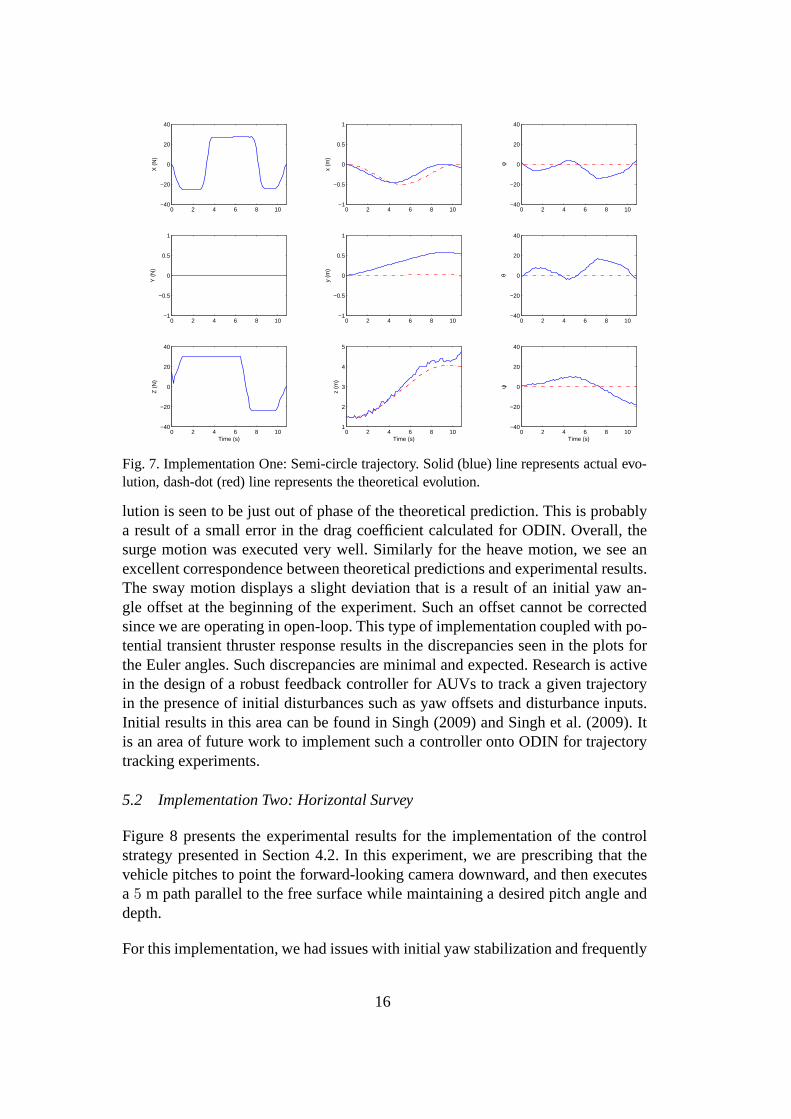
Figure 7 displays the implementation results of the controlstrategy given in Table3 executed by ODIN. The first column of plots in Fig. 7 give the pertinent controlforces (in Newtons) and control moments (in Newton meters) that were appliedby ODIN during the implementation. In the second and third columns, we presentthe evolution of the vehicle during the test. The solid (blue) line denotes the actualevolution of ODIN. The dash-dot (red) line represents the theoretical evolution ofODIN.

We first examine the controls applied during the experiment.Note that forX, themagnitude of the control does not quite match the value givenin Table 3. This isa result of implementing a six-dimensional control strategy onto a vehicle that isdriven by eight thrusters. The linear transformation applied to convert from six di-mensions to eight dimensions, and vise-versa, has a nonzeronull space. This meansthat there are infinitely many transformations which convert the controls. ODIN’son-board computer choses one of these transformations for its computations. Moreinformation regarding this transformation can be found in Smith (2008), with spe-cific details related to ODIN found in Hanai et al. (2003). Thesmall applied thrustsseen forσ2 can also be attributed to this transformation.

Next, consider the evolution of ODIN during the experiment.The main intent ofthis strategy was to realize both heave and surge motions. For the surge motion, theexperimental results match well with the theoretical trajectory. We see deviationbetween the actual and theoretical evolutions begin aroundt = 4 seconds. Thisoccurs because ODIN did not reach the full0.5 m displacement. The actual evo-

15

0 2 4 6 8 10−40

−20

0

20

40

X (

N)

0 2 4 6 8 10−1

−0.5

0

0.5

1

Y (

N)

0 2 4 6 8 10−40

−20

0

20

40

Z (

N)

Time (s)

0 2 4 6 8 10−1

−0.5

0

0.5

1

x (m

)0 2 4 6 8 10

−1

−0.5

0

0.5

1

y (m

)

0 2 4 6 8 101

2

3

4

5

z (m

)

Time (s)

0 2 4 6 8 10−40

−20

0

20

40

φ

0 2 4 6 8 10−40

−20

0

20

40

θ

0 2 4 6 8 10−40

−20

0

20

40

ψ

Time (s)

Fig. 7. Implementation One: Semi-circle trajectory. Solid(blue) line represents actual evo-lution, dash-dot (red) line represents the theoretical evolution.

lution is seen to be just out of phase of the theoretical prediction. This is probablya result of a small error in the drag coefficient calculated for ODIN. Overall, thesurge motion was executed very well. Similarly for the heavemotion, we see anexcellent correspondence between theoretical predictions and experimental results.The sway motion displays a slight deviation that is a result of an initial yaw an-gle offset at the beginning of the experiment. Such an offsetcannot be correctedsince we are operating in open-loop. This type of implementation coupled with po-tential transient thruster response results in the discrepancies seen in the plots forthe Euler angles. Such discrepancies are minimal and expected. Research is activein the design of a robust feedback controller for AUVs to track a given trajectoryin the presence of initial disturbances such as yaw offsets and disturbance inputs.Initial results in this area can be found in Singh (2009) and Singh et al. (2009). Itis an area of future work to implement such a controller onto ODIN for trajectorytracking experiments.

5.2 Implementation Two: Horizontal Survey

Figure 8 presents the experimental results for the implementation of the controlstrategy presented in Section 4.2. In this experiment, we are prescribing that thevehicle pitches to point the forward-looking camera downward, and then executesa 5 m path parallel to the free surface while maintaining a desired pitch angle anddepth.

For this implementation, we had issues with initial yaw stabilization and frequently

16

0 10 20 30 40−20

−15

−10

−5

0

5

10

X (

N)

0 10 20 30 40−1

−0.5

0

0.5

1

Y (

N)

0 10 20 30 40−5

0

5

M (

N m

)

Time (s)

0 10 20 30 40−6

−5

−4

−3

−2

−1

0

1

x (m

)0 10 20 30 40

−4

−2

0

2

4

y (m

)

0 10 20 30 400

0.5

1

1.5

2

2.5

3

z (m

)

Time (s)

0 10 20 30 40−40

−20

0

20

40

φ

0 10 20 30 40−40

−20

0

20

40

θ

0 10 20 30 40−40

−20

0

20

40

ψ

Time (s)

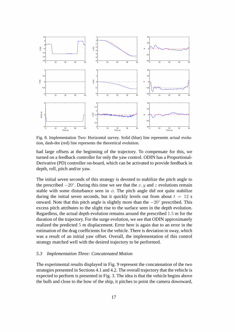
Fig. 8. Implementation Two: Horizontal survey. Solid (blue) line represents actual evolu-tion, dash-dot (red) line represents the theoretical evolution.

had large offsets at the beginning of the trajectory. To compensate for this, weturned on a feedback controller for only the yaw control. ODIN has a Proportional-Derivative (PD) controller on-board, which can be activated to provide feedback indepth, roll, pitch and/or yaw.

The initial seven seconds of this strategy is devoted to stabilize the pitch angle tothe prescribed−20. During this time we see that thex, y andz evolutions remainstable with some disturbance seen inφ. The pitch angle did not quite stabilizeduring the initial seven seconds, but it quickly levels out from aboutt = 12 sonward. Note that this pitch angle is slightly more than the−20 prescribed. Thisexcess pitch attributes to the slight rise to the surface seen in the depth evolution.Regardless, the actual depth evolution remains around the prescribed1.5 m for theduration of the trajectory. For the surge evolution, we see that ODIN approximatelyrealized the predicted5 m displacement. Error here is again due to an error in theestimation of the drag coefficients for the vehicle. There isdeviation in sway, whichwas a result of an initial yaw offset. Overall, the implementation of this controlstrategy matched well with the desired trajectory to be performed.

5.3 Implementation Three: Concatenated Motion

The experimental results displayed in Fig. 9 represent the concatenation of the twostrategies presented in Sections 4.1 and 4.2. The overall trajectory that the vehicle isexpected to perform is presented in Fig. 3. The idea is that the vehicle begins abovethe bulb and close to the bow of the ship, it pitches to point the camera downward,

17

0 10 20 30 40 50−40

−20

0

20

40

X (

N)

0 10 20 30 40 50−40

−20

0

20

40

Z (

N)

0 10 20 30 40 50−5

0

5

M (

N m

)

Time (s)

0 10 20 30 40 50−6

−5

−4

−3

−2

−1

0

1

x (m

)0 10 20 30 40 50

−4

−2

0

2

4

y (m

)

0 10 20 30 40 501

2

3

4

5

6

z (m

)

Time (s)

0 10 20 30 40 50−40

−20

0

20

40

φ

0 10 20 30 40 50−40

−20

0

20

40

θ

0 10 20 30 40 50−50

0

50

ψ

Time (s)

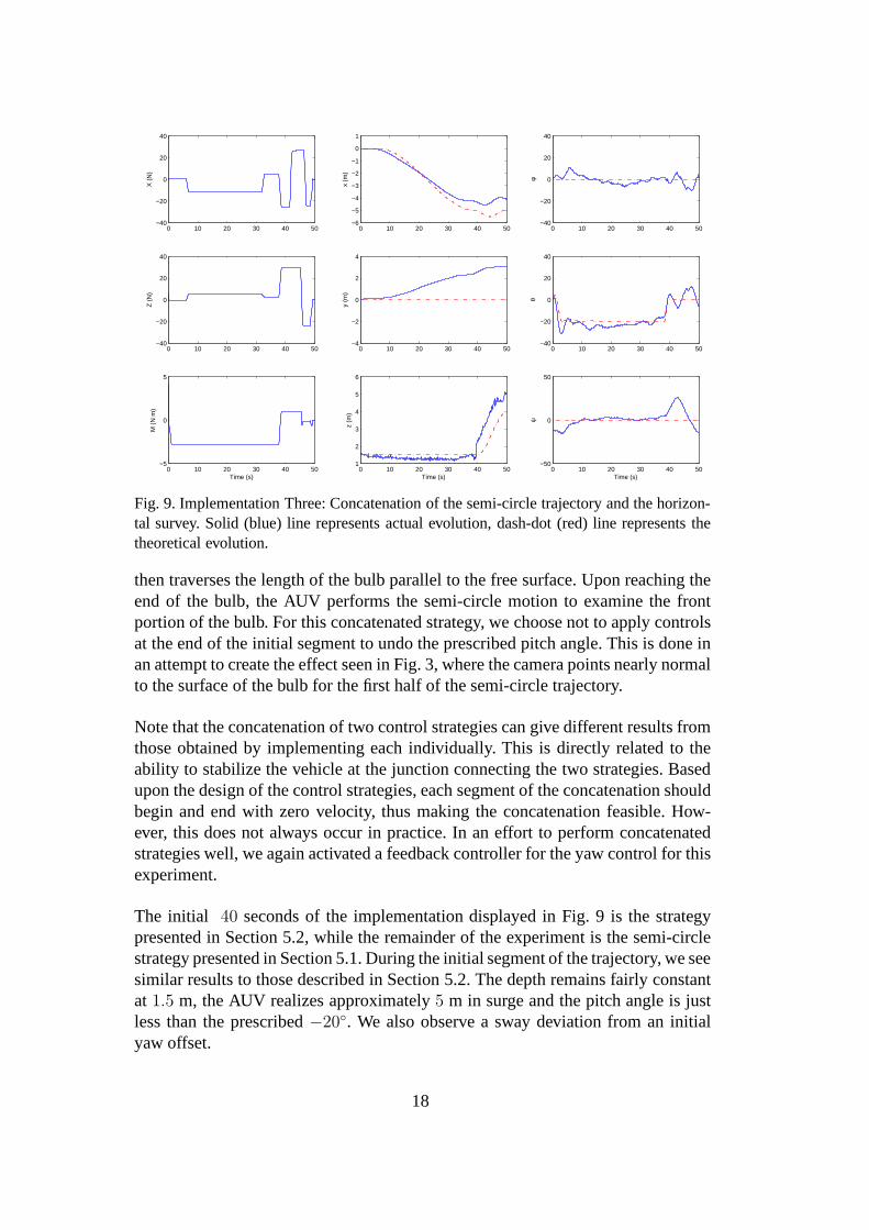
Fig. 9. Implementation Three: Concatenation of the semi-circle trajectory and the horizon-tal survey. Solid (blue) line represents actual evolution,dash-dot (red) line represents thetheoretical evolution.

then traverses the length of the bulb parallel to the free surface. Upon reaching theend of the bulb, the AUV performs the semi-circle motion to examine the frontportion of the bulb. For this concatenated strategy, we choose not to apply controlsat the end of the initial segment to undo the prescribed pitchangle. This is done inan attempt to create the effect seen in Fig. 3, where the camera points nearly normalto the surface of the bulb for the first half of the semi-circletrajectory.

Note that the concatenation of two control strategies can give different results fromthose obtained by implementing each individually. This is directly related to theability to stabilize the vehicle at the junction connectingthe two strategies. Basedupon the design of the control strategies, each segment of the concatenation shouldbegin and end with zero velocity, thus making the concatenation feasible. How-ever, this does not always occur in practice. In an effort to perform concatenatedstrategies well, we again activated a feedback controller for the yaw control for thisexperiment.

The initial 40 seconds of the implementation displayed in Fig. 9 is the strategypresented in Section 5.2, while the remainder of the experiment is the semi-circlestrategy presented in Section 5.1. During the initial segment of the trajectory, we seesimilar results to those described in Section 5.2. The depthremains fairly constantat 1.5 m, the AUV realizes approximately5 m in surge and the pitch angle is justless than the prescribed−20. We also observe a sway deviation from an initialyaw offset.

18

Examining the remaining20 seconds of the implemented strategy, we see behav-ior similar to that presented in Section 5.1, with the exception that the error fromthe first segment of the trajectory is introduced as the initial condition for the sec-ond leg of the concatenated motion. We see the initial negative surge of0.5 mfollowed by a positive surge evolution of approximately0.5 m, as prescribed. Thedepth evolution shows an overshoot in depth by about1 m. The pitch evolutionafter40 seconds oscillates about zero with a magnitude less than tendegrees. Thisis a result of not stabilizing the pitch angle to zero before beginning the semi-circletrajectory. Here, the vehicle is simple relying on the righting arm to return it to anupright position. The oscillations present in roll are an artifact of the small distancebetween the center of gravity and center of buoyancy, i.e., small righting arm. Thisconfiguration provides a very controllable vehicle in the sense that it can realizemany configurations by use of the on-board thrusts, however this results in a de-crease in stability of the AUV. Hence, reduced stability coupled with the open-loopimplementation results in the expectation of small perturbations and oscillations inthe evolution of the vehicle. The yaw evolution begins with an initial offset that isremedied within the first10 seconds. Note that this deviation arises during the timethat the pitch control operating. Att = 40 s, we again notice a spike in the yaw,which corresponds to a time when the vehicle is releasing thepitch angle.

6 Conclusions

In this paper, we have presented the equations of motion governing the submergedrigid body in both a standard form as well as a form utilizing the architecture ofdifferential geometry. By use of these geometric equations, we are able to providesolutions to the motion planning problem for AUVs via a geometric reduction andexamination of the decoupling vector fields for the system. This geometric controltheory technique has been proven to be an effective path planning tool for AUVs,especially those operating in an under-actuated condition, see e.g., Smith (2008)and Smith et al. (2009). Here, we considered a direct application of this path plan-ning technique to examine the bulbous bow of ships.

Due to the unique shape and location, examination and surveyof the bulbous bowprovides an interesting motion planning problem for the submerged rigid body. Wedo not provide an exhaustive survey algorithm, but propose two control strategieswhich can be used to examine the majority of the bulb itself. For implementationpurposes, the experiments presented here have been scaled down and assume ageneral form of the bulb. Trajectories to examine an actual bulbous bow of a shipwould need to be generated for the specific size and shape of the bulb. The intenthere is to present an application of an emerging technique inthe area of motionplanning for the submerged rigid body.

The experimental results presented here extend the work developed in Smith (2008),and further validate the design of implementable control strategies by use of differ-ential geometric techniques. This architecture is not justa change of notation for

19

the same equations of motion, but a presentation with a much richer inherent struc-ture. A structure which can be exploited for autonomous pathplanning in the eventof a disabled vehicle (under-actuated) or used to guide the design of future AUVs.Research is currently ongoing to migrate the techniques presented here from thetest-bed vehicle ODIN onto an AUV active in the open ocean. The ability to re-produce great implementation results such as those presented here gives us a goodstart to investigate the potential of actual sea trials.

The excellent correlation between theoretical predictions and experimental resultsshown in this paper are a result of working in a well-known andcontrolled en-vironment. Many years and experimental trials have given usinformation on thespecifics of the pool environment and we are able to limit uncertainties during theexperiments. This will definitely not be the case in the ocean. To move from thepool to the ocean, significant adjustments will be necessary. First off, an AUV can-not operate strictly in an open-loop mode. Poorly known disturbance forces, suchas ocean currents, are too large and unpredictable to be neglected or accounted fora priori. In an open-loop implementation in the ocean, we would expect to see largeerrors between theoretical predictions and experimental results.

A reasonable approach to begin the migration is to use our trajectories as the de-sired theoretical predictions, and implement a robust, feedback trajectory-trackingcontroller that can compensate for the external disturbances. Initial steps in this di-rection have been taken, and results can be found in Singh et al. (2009) and Sanyaland Chyba (2009). Once the theory contained in these references becomes well-developed and proven technology, we plan to implement a hybrid control schemeonto ODIN in the pool. We will begin with simple disturbances, such as initial devi-ations in the state of the vehicle. From the discussion presented in Sections 5.1-5.3,a known source of error comes from an initial offset in the vehicle’s configuration,typically in yaw. Implementing a hybrid controller as previously described will re-quire many upgrades to ODIN, or the use of an alternate AUV forsea trials.

This brings up the natural question regarding the applicability of the presented tech-niques to multiple types of underwater vehicles. First, thetheoretical aspect, namelythe geometric control, is independent of the choice of the vehicle. The geometrictheory is solely based on the fact the underwater vehicle is an example of a simplemechanical control system; this is true for any underwater vehicle. Generalizing ourwork to alternate vehicle designs requires only slight modifications. If the vehiclehas three planes of symmetry, which is common for AUVs, the basic foundationsand formulations do not change. Obviously, the physical attributes, such as mass,inertia and added mass, need to be altered. This correspondsto the generation ofa new kinetic energy metric for the kinematic reduction. Viscous drag coefficientsneed to be estimated for the specific vehicle, and the locations of the center ofbuoyancy and center of gravity need to be calculated to appropriately account forthe restoration forces and moments. Aside from the obvious physical properties,the only major difference is changing the input control vector fields. These are the

20

basis upon which the decoupling vector fields, and hence the kinematic motions,are determined. This alteration is simply done by expressing the location and out-put of the actuators of the vehicle in the geometric formulation. In Smith (2008),the reader can find the generalization of the techniques presented here to two otherunderwater vehicles.

References

Allmendinger, E. E., 1990. Submersible Vehicle Design. SNAME.Ardema, M. D., 2005. Newton-Euler Dynamics. Springer, New York.Bhattacharyya, R., 1978. Dynamics of Marine Vehicles. JohnWiley & Sons.Bullo, F., 2004. Trajectory design for mechanical systems:From geometry to algo-

rithms. European Journal of Control 10(5), 397–410.Bullo, F., Leonard, N., Lewis, A., 2000. Controllability and motion algorithms for

underactuated lagrangian systems on lie groups. Instituteof Electrical and Elec-tronics Engineers. Transactions on Automatic Control 45(8), 1437–1454.

Bullo, F., Lewis, A. D., 2005. Geometric Control of Mechanical Systems. Springer.Bullo, F., Lynch, K., 2001. Kinematic controllability for decoupled trajectory plan-

ning in underactuated mechanical systems. IEEE Transactions. Robotics and Au-tomation 17 (4), 402–412.

Chyba, M., Choi, S., Haberkorn, T., Smith, R. N., Zhao, S., 2006. Towards practi-cal implementation of time optimal trajectories for underwater vehicles. In: Pro-ceedings of the 25th International Conference on Offshore Mechanics and ArcticEngineering.

Chyba, M., Haberkorn, T., Smith, R., Wilkens, G., 2009a. A geometrical analysisof trajectory design for underwater vehicles. Discrete andContinuous DynamicalSystems-B 11(2).

Chyba, M., Haberkorn, T., Smith, R. N., Choi, S., 2008. Design and implementationof time efficient trajectories for an underwater vehicle. Ocean Engineering 35 (1),63–76.

Chyba, M., Haberkorn, T., Smith, R. N., Singh, S., Choi, S., 2009b. Increasing un-derwater vehicle autonomy by reducing energy consumption.Ocean Engineer-ing: Special Edition on AUVs 36(1), 62–73.

Chyba, M., Smith, R. N., 2008. A first extension of geometric control theory tounderwater vehicles. In: Proceedings of the 2008 IFAC Workshop on Navigation,Guidance and Control of Underwater Vehicles. Killaloe, Ireland, Vol. 2, Part 1.

Fossen, T. I., 1994. Guidance and Control of Ocean Vehicles.John Wiley & Sons.GlobalSecurity.org, 2008. USS George H.W. Bush.http://www.globalsecurity.org/military/systems/ship/bulbous-bow.htm, viewed May 2008.

Hanai, A., Choi, H., Choi, S., Yuh, J., 2003. Minimum energy based fine motioncontrol of underwater robots in the presence of thruster nonlinearity. In: Proceed-ings of IEEE/RSJ International Conference on Intelligent Robots and Systems.Las Vegas, Nevada, USA, pp. 559–564.

21

Imlay, F., 1961. The complete expressions for added mass of arigid body movingin an ideal fluid. Technical Report DTMB 1528, David Taylor Model Basin,Washington D.C.

Lamb, H., 1945. Hydrodynamics,6th Edition. Dover Publications.Lamb, H., 1961. Dynamics. University Press, Cambridge.Leonard, N., Krishnaprasad, P., 1995. Motion control of drift-free, left-invariant

systems on lie groups. IEEE Transactions on Automatic Control 40(9), 1539–1554.

Leonard, N. E., 1995. Periodic forcing, dynamics and control of underactuatedspacecraft and underwater vehicles. In: Proceedings of the34th IEEE Confer-ence on Decision and Control. New Orleans, Louisiana, pp. 3980–3985.

Meriam, J., Kraige, L., 1997. Engineering Mechanics, DYNAMICS, 4th Edition.John Wiley & Sons, Inc., New York.

Newman, J., 1977. Marine Hydrodynamics. MIT Press, Cambridge, MA.Rijkaart, P., 2008. M/V Eurodam.http://gcaptain.com/maritime/blog/tag/eurodam/, viewed March 2009.

Sanyal, A., Chyba, M., 2009. Robust feedback tracking of autonomous underwatervehicles with disturbance rejection. In: Proceedings of the American ControlConference (ACC). St. Louis, MO, to appear.

Singh, S., Sanyal, A., Smith, R., Nordkvist, N., Chyba, M., 2009. Robust trackingcontrol of autonomous underwater vehicles in presence of disturbance inputs. In:Proceedings of the 28th International Conference on Offshore Mechanics andArtic Engineering (OMAE). Honolulu, Hawaii.

Singh, S. B., 2009. Almost global feedback control of autonomous underwater ve-hicles. Master’s thesis, University of Hawai‘i at Manoa.

Smith, R. N., 2008. Geometric control theory and its application to underwatervehicles. Ph.D. thesis, University of Hawai‘i at Manoa.

Smith, R. N., Chyba, M., Singh, S. B., 2008. Submerged rigid body subject todissipative and potential forces. In: Proceedings of the IEEE Region 10 Collo-quium and Third International Conference on Industrial andInformation Sys-tems. Kharagpur, India.

Smith, R. N., Chyba, M., Wilkens, G. R., Catone, C. J., 2009. Ageometrical ap-proach to the motion planning problem for a submerged rigid body. InternationalJournal of Control.Accepted, to appear.

SNAME, 1950. Nomenclature for treating the motion of a submerged body througha fluid. Technical and Research Bulletin No. 1-5, The Societyof Naval Architectsand Marine Engineers.

22