tr 103 293 - v1.1.1 - broadband radio access networks ... · pdf filebroadband radio access...

ETSI TR 103 293 V1.1.1 (2015-07)

Broadband Radio Access Networks (BRAN); Broadband Wireless Access and Backhauling

for Remote Rural Communities

TECHNICAL REPORT

ETSI

ETSI TR 103 293 V1.1.1 (2015-07) 2

Reference DTR/BRAN-0040010

Keywords access, BWA

ETSI

650 Route des Lucioles F-06921 Sophia Antipolis Cedex - FRANCE

Tel.: +33 4 92 94 42 00 Fax: +33 4 93 65 47 16

Siret N° 348 623 562 00017 - NAF 742 C

Association à but non lucratif enregistrée à la Sous-Préfecture de Grasse (06) N° 7803/88

Important notice

The present document can be downloaded from: http://www.etsi.org/standards-search

The present document may be made available in electronic versions and/or in print. The content of any electronic and/or print versions of the present document shall not be modified without the prior written authorization of ETSI. In case of any

existing or perceived difference in contents between such versions and/or in print, the only prevailing document is the print of the Portable Document Format (PDF) version kept on a specific network drive within ETSI Secretariat.

Users of the present document should be aware that the document may be subject to revision or change of status. Information on the current status of this and other ETSI documents is available at

http://portal.etsi.org/tb/status/status.asp

If you find errors in the present document, please send your comment to one of the following services: https://portal.etsi.org/People/CommiteeSupportStaff.aspx

Copyright Notification

No part may be reproduced or utilized in any form or by any means, electronic or mechanical, including photocopying and microfilm except as authorized by written permission of ETSI.

The content of the PDF version shall not be modified without the written authorization of ETSI. The copyright and the foregoing restriction extend to reproduction in all media.

© European Telecommunications Standards Institute 2015.

All rights reserved.

DECTTM, PLUGTESTSTM, UMTSTM and the ETSI logo are Trade Marks of ETSI registered for the benefit of its Members. 3GPPTM and LTE™ are Trade Marks of ETSI registered for the benefit of its Members and

of the 3GPP Organizational Partners. GSM® and the GSM logo are Trade Marks registered and owned by the GSM Association.

http://www.etsi.org/standards-search

http://portal.etsi.org/tb/status/status.asp

https://portal.etsi.org/People/CommiteeSupportStaff.aspx

ETSI

ETSI TR 103 293 V1.1.1 (2015-07) 3

Contents Intellectual Property Rights ................................................................................................................................ 5

Foreword ............................................................................................................................................................. 5

Modal verbs terminology .................................................................................................................................... 5

Introduction ........................................................................................................................................................ 5

1 Scope ........................................................................................................................................................ 6

2 References ................................................................................................................................................ 6

2.1 Normative references ......................................................................................................................................... 6

2.2 Informative references ........................................................................................................................................ 6

3 Definitions and abbreviations ................................................................................................................... 7

3.1 Definitions .......................................................................................................................................................... 7

3.2 Abbreviations ..................................................................................................................................................... 7

4 Technical scenarios and architecture ........................................................................................................ 9

4.1 Technical scenarios ............................................................................................................................................ 9

4.1.1 Introduction................................................................................................................................................... 9

4.1.2 Traffic characteristics ................................................................................................................................. 10

4.1.3 Deployment constraints .............................................................................................................................. 10

4.2 Radio transport technologies ............................................................................................................................ 10

4.2.1 Introduction................................................................................................................................................. 10

4.2.2 WiLD (WiFi-based Long Distance) networks ............................................................................................ 10

4.2.3 WiMAX (Worldwide Interoperability for Microwave Access) .................................................................. 11

4.2.4 VSAT .......................................................................................................................................................... 11

4.3 Architecture example ....................................................................................................................................... 12

4.3.1 Overview .................................................................................................................................................... 12

4.3.2 Network Controller ..................................................................................................................................... 12

4.3.3 Access Network .......................................................................................................................................... 13

4.3.4 Satellite backhaul scenario .......................................................................................................................... 13

5 Optimization and monitoring of HNB network...................................................................................... 13

5.1 Introduction ...................................................................................................................................................... 13

5.1.1 Rural deployment scenarios for HNB ......................................................................................................... 13

5.1.2 Network self-configuration procedures ...................................................................................................... 14

5.1.2.1 Bounding coverage................................................................................................................................ 14

5.1.2.2 Detection of new neighbours................................................................................................................. 14

5.1.2.3 Frequency and primary scrambling code selection ............................................................................... 15

5.1.3 Long-term traffic-aware self-optimization procedures ............................................................................... 15

5.1.4 Criteria for switching on/off HNBs ............................................................................................................ 15

5.1.5 Dynamic cell range expansion .................................................................................................................... 16

6 Interoperability of access and transport network .................................................................................... 16

6.1 General ............................................................................................................................................................. 16

6.2 Traffic offloading ............................................................................................................................................. 17

6.3 Network architectures and benefits of traffic offloading .................................................................................. 17

6.4 Implementations in 3GPP networks ................................................................................................................. 18

6.4.1 Offloading implementations complying with the 3GPP standard ............................................................... 18

6.4.2 Non-standard offloading implementations: data traffic caching over satellite ........................................... 18

6.4.2.1 Introduction ........................................................................................................................................... 18

6.4.2.2 Content caching ..................................................................................................................................... 19

6.4.2.3 Content caching tests in Peru ................................................................................................................ 20

6.4.2.4 One VSAT working in a controlled environment ................................................................................. 20

6.4.2.5 Multiple VSATs .................................................................................................................................... 21

6.5 Access network and backhaul interplay ........................................................................................................... 23

6.5.1 3GPP background ....................................................................................................................................... 23

6.5.2 Structure of the AN-BH interface ............................................................................................................... 24

6.5.3 Information requirement for AN algorithms ............................................................................................... 25

ETSI

ETSI TR 103 293 V1.1.1 (2015-07) 4

7 Backhaul aware scheduling .................................................................................................................... 26

7.1 Backhaul-aware scheduling with a single HNB ............................................................................................... 26

7.1.1 Overview .................................................................................................................................................... 26

7.1.2 Downlink scheduling .................................................................................................................................. 26

7.1.2.1 System description and assumptions ..................................................................................................... 26

7.1.2.2 Simulation results .................................................................................................................................. 27

7.1.3 Uplink scheduling ....................................................................................................................................... 28

7.1.3.1 System description and assumptions ..................................................................................................... 28

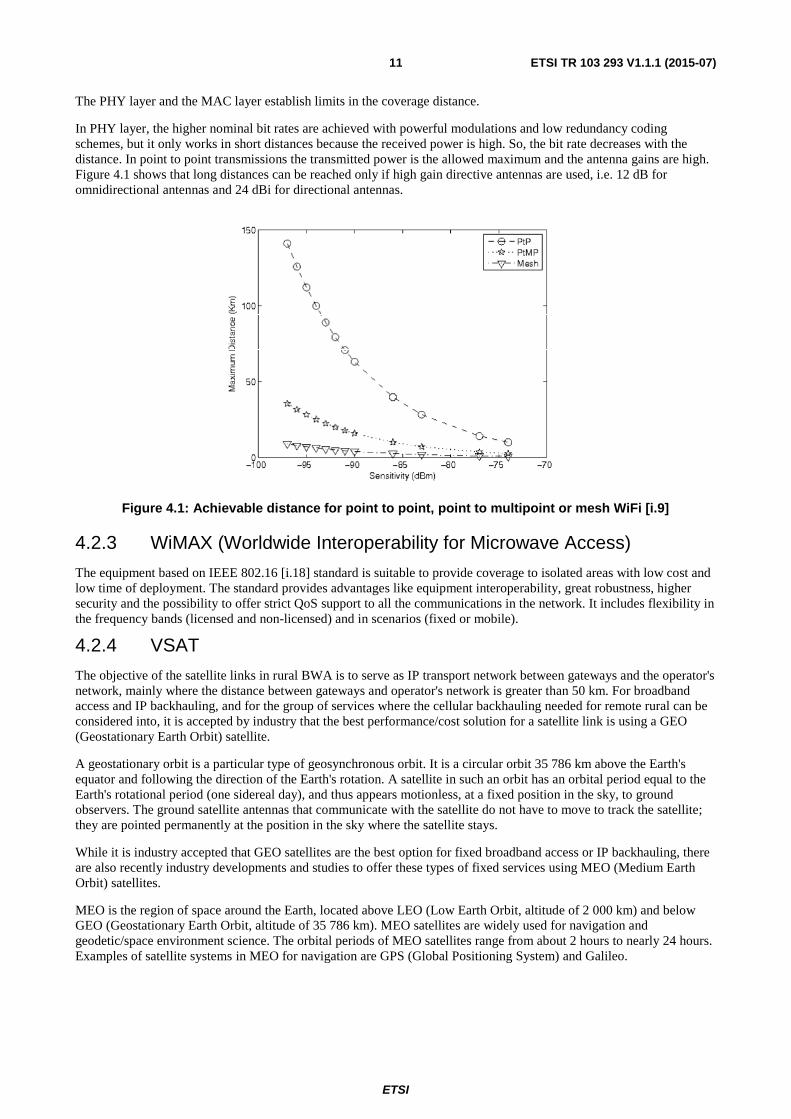
7.1.3.2 Simulation results .................................................................................................................................. 29

7.2 Backhaul aware scheduling with multiple HNBs ............................................................................................. 30

7.2.1 Overview .................................................................................................................................................... 30

7.2.2 Resource allocation (rate, power and number of codes) for multiple HNBs .............................................. 31

7.2.3 Downlink resource allocation for multiple HNBs ...................................................................................... 31

7.2.4 Uplink resource allocation for multiple HNBs ........................................................................................... 33

7.3 Congestion Detection and Measurement .......................................................................................................... 34

7.3.1 Introduction................................................................................................................................................. 34

7.3.2 Analysis of a deployment case .................................................................................................................... 34

7.3.2.1 Delay ..................................................................................................................................................... 34

7.3.2.2 Frame loss ............................................................................................................................................. 35

8 Backhaul network ................................................................................................................................... 36

8.1 Multi-hop solution for backhaul of rural 3G/4G access networks .................................................................... 36

9 Interface between the Access Network and the Backhaul Network ....................................................... 38

9.1 Interface overview: elements and procedures involved .................................................................................... 38

9.1.1 Introduction................................................................................................................................................. 38

9.1.2 Architecture ................................................................................................................................................ 38

9.2 BH state information collection ........................................................................................................................ 39

9.2.1 AN algorithms requirements ....................................................................................................................... 39

9.3 Formal definition of the interface ..................................................................................................................... 40

9.3.1 Background ................................................................................................................................................. 40

9.3.2 Service provided by the protocol ................................................................................................................ 40

9.3.3 Entities involved in the protocol ................................................................................................................. 40

9.3.4 Information exchanged between entities ..................................................................................................... 40

9.3.4.1 ACK Message ....................................................................................................................................... 40

9.3.4.2 Information Request Message ............................................................................................................... 40

9.3.4.3 Bandwidth Availability Request Message ............................................................................................ 40

9.3.4.4 Information Indication Message............................................................................................................ 41

9.3.5 Message format ........................................................................................................................................... 41

Annex A: Simulation methodology ....................................................................................................... 42

A.1 Introduction ............................................................................................................................................ 42

A.2 Reference scenario and simulation parameters ...................................................................................... 42

A.3 Power consumption model and battery dynamics .................................................................................. 43

A.4 Energy harvesting model ........................................................................................................................ 44

A.5 Daily traffic profile ................................................................................................................................. 44

History .............................................................................................................................................................. 47

ETSI

ETSI TR 103 293 V1.1.1 (2015-07) 5

Intellectual Property Rights IPRs essential or potentially essential to the present document may have been declared to ETSI. The information pertaining to these essential IPRs, if any, is publicly available for ETSI members and non-members, and can be found in ETSI SR 000 314: "Intellectual Property Rights (IPRs); Essential, or potentially Essential, IPRs notified to ETSI in respect of ETSI standards", which is available from the ETSI Secretariat. Latest updates are available on the ETSI Web server (http://ipr.etsi.org).

Pursuant to the ETSI IPR Policy, no investigation, including IPR searches, has been carried out by ETSI. No guarantee can be given as to the existence of other IPRs not referenced in ETSI SR 000 314 (or the updates on the ETSI Web server) which are, or may be, or may become, essential to the present document.

Foreword This Technical Report (TR) has been produced by ETSI Technical Committee Broadband Radio Access Networks (BRAN).

Modal verbs terminology In the present document "shall", "shall not", "should", "should not", "may", "need not", "will", "will not", "can" and "cannot" are to be interpreted as described in clause 3.2 of the ETSI Drafting Rules (Verbal forms for the expression of provisions).

"must" and "must not" are NOT allowed in ETSI deliverables except when used in direct citation.

Introduction Broadband access for rural communities is one of the objectives of the European Commission. The EC FP7 project ICT-601102 STP TUCAN3G, "Wireless technologies for isolated rural communities in developing countries based on cellular 3G femtocell deployments" has addressed this problem and has provided a system design for deployments of Telefonica in Peru.

The present document includes the main outcome of the project.

http://webapp.etsi.org/IPR/home.asp

http://portal.etsi.org/Help/editHelp!/Howtostart/ETSIDraftingRules.aspx

ETSI

ETSI TR 103 293 V1.1.1 (2015-07) 6

1 Scope The present document describes the architecture and implementation guidance for rural BWA based on 3G femto base stations, and a variety of terrestrial and satellite backhaul solutions. The implementation guidance includes self-optimization of physical layer parameters and recommendations for femto-to-femto and femto-to-backhaul interaction. Additionally, deployment examples, at least for Peru, are included.

2 References

2.1 Normative references References are either specific (identified by date of publication and/or edition number or version number) or non-specific. For specific references, only the cited version applies. For non-specific references, the latest version of the reference document (including any amendments) applies.

Referenced documents which are not found to be publicly available in the expected location might be found at http://docbox.etsi.org/Reference.

NOTE: While any hyperlinks included in this clause were valid at the time of publication, ETSI cannot guarantee their long term validity.

The following referenced documents are necessary for the application of the present document.

Not applicable.

2.2 Informative references

References are either specific (identified by date of publication and/or edition number or version number) or non-specific. For specific references, only the cited version applies. For non-specific references, the latest version of the reference document (including any amendments) applies.

NOTE: While any hyperlinks included in this clause were valid at the time of publication, ETSI cannot guarantee their long term validity.

The following referenced documents are not necessary for the application of the present document but they assist the user with regard to a particular subject area.

[i.1] Lee K., Lee J., Yi Y., Rhee I. & Chong S.: "Mobile data offloading: how much can WiFi deliver?". In Proceedings of the 6th International COnference (p. 26). ACM, November 2010.

[i.2] Lin Y., B. Gan, C. H. & Liang C. F.: "Reducing call routing cost for femtocells". IEEE Transactions on Wireless Communications, pp. 2302-2309, vol. 9, no. 7, July 2010.

[i.3] Zdarsky F., A. Maeder, A. Al-Sabea, S. & Schmid S.: "Localization of data and control plane traffic in enterprise femtocell networks". In Proceedings of the 73rd IEEE Conference on Vehicular Technology (VTC Spring), pp. 1-5, May 2011.

[i.4] Khan M., F. Khan M. I. & Raahemifar K.: "Local IP Access (LIPA) enabled 3G and 4G femtocell architectures". In Proceedings of the 24th IEEE Canadian Conference on Electrical and Computer Engineering (CCECE), pp. 1049-1053, May 2011.

[i.5] Small Cell Forum Release Two documents.

NOTE: Available online at http://www.scf.io/en/index.php?utm_campaign=Release%2520Two.

[i.6] 3GPP TS 23.829: "3GPP; Technical Specification Group Services and System Aspects; Local IP Access and Selected IP Traffic Offload (LIPA-SIPTO)" - Release 10.

[i.7] TUCAN3G D42: "Optimization and monitoring of HNB network", November 2014.

NOTE: Available at http://www.ict-tucan3g.eu/.

http://docbox.etsi.org/Reference

http://www.scf.io/en/index.php?utm_campaign=Release%2520Two

http://www.ict-tucan3g.eu/

ETSI

ETSI TR 103 293 V1.1.1 (2015-07) 7

[i.8] TUCAN3G D41: "UMTS/HSPA network dimensioning", November 2013.


[i.9] TUCAN3G D51: "Technical requirements and evaluation of WiLD, WIMAX and VSAT for backhauling rural femtocells networks", October 2013.


[i.10] TUCAN3G D52: "Heterogeneous transport network testbed deployed and validated in laboratory", April 2014.


[i.11] Recommendation ITU-T G.114: "One way transmission time", May 2003.

[i.12] 3GPP TR 25.853: "Delay Budget within the access stratum".

[i.13] ETSI TS 125 467: "Universal Mobile Telecommunications System (UMTS); UTRAN architecture for 3G Home Node B (HNB); Stage 2 (3GPP TS 25.467)".

[i.14] ETSI TS 123 207: "Digital cellular telecommunications system (Phase 2+); Universal Mobile Telecommunications System (UMTS); End-to-end Quality of Service (QoS) concept and architecture (3GPP TS 23.207 version 6.6.0 Release 6)".

[i.15] ETSI TS 125 444: "Universal Mobile Telecommunications System (UMTS); Iuh data transport (3GPP TS 25.444 version 11.0.0 Release 11)".

[i.16] ETSI TS 133 320: "Universal Mobile Telecommunications System (UMTS); LTE; Security of Home Node B (HNB) / Home evolved Node B (HeNB) (3GPP TS 33.320 version 12.1.0 Release 12)".

[i.17] IEEE 802.11™: "IEEE Standard for Information technology--Telecommunications and information exchange between systems Local and metropolitan area networks--Specific requirements Part 11: Wireless LAN Medium Access Control (MAC) and Physical Layer (PHY) Specifications".

[i.18] IEEE 802.16™: "IEEE Standard for Air Interface for Broadband Wireless Access Systems".

[i.19] TUCAN3G D43: "Interoperability of access and transport network", April 2013.


3 Definitions and abbreviations

3.1 Definitions For the purposes of the present document, the following terms and definitions apply:

heterogeneous network: network consisting of cells with different sized coverage areas, possibly overlapping and possibly of different wireless technologies

Location Area Code (LAC): code to group cells together for circuit-switched mobility purposes

WiFi™: Technology based on IEEE 802.11 [i.17] standard.

WiMAX™: Technology based on IEEE 802.16 [i.18] standard.

3.2 Abbreviations For the purposes of the present document, the following abbreviations apply:

ABI Access-Backhaul interface AC Access Controller





ETSI

ETSI TR 103 293 V1.1.1 (2015-07) 8

ACK Acknowledgement ADSL Asymetrical Digital Subscriber Line AICH Acquisition Indicator Channel AMC Adaptive Modulation and Coding AN Access Network ATM Asynchroneous Transfer Mode AWGN Additive White Gaussian Noise BH Backhaul BS Base Station BWA Broadband Wireless Access CAPEX Capital Expenditure CDMA Code Division Multiple Access CPE Customer Premises Equipment CRE Cell Range Extension CRL Certificate Revocation List CS Circuit Switched DivServ Differential Services DL Downlink DNS Domain Name System DSCP Differentiated Services Code Point ECM EPS Connection Management eNB Evolved Node B EPC Evolved Packet Core EPS Evolved Packet System Er Erlang E-UTRAN Evolved UMTS Terrestrial Radio Access Network FCAP Frequency and Code Assignment Problem GCP Graph Colouring Problem GEO Geostationary Earth Orbit GGSN Gateway GPRS Service Node GPS Global Position System GW Gateway HetNet Heterogeneous Network HMS HNB Management System HNB Home Node B HNB-GW Home Node B Gateway HNBAP HNB Application Protocol HSDPA High Speed Downlink Packet Access IP Internet Protocol IPsec IP security scheme ISP Internet Service Provider Iuh Iu home KPI Key Performance Indicator LAC Location Area Code LEO Low Earth Orbit LIPA Local IP Access LTE Long Term Evolution MDT Minimization Drive Tests MEO Medium Earth Orbit MPLS Multi Protocol Label Switching NCell Neighbour Cell NCL Neighbour Cell List NOS Network Orchestration System NP Non Polynomial NRT Neighbour Routing Table NTP Network Time Protocol NWL Network Listen OPC Optimal Power and Code allocation OPEX Operational Expenditure PCI Physical Cell Identity (LTE equivalent of the 3G PSC) P-CPICH Primary Common Pilot Channel PDP Packet Data Protocol

ETSI

ETSI TR 103 293 V1.1.1 (2015-07) 9

PF Proportional Fair PLMN Public Land Mobile Network PM Performance Management PS Packet Switched PSC Primary scrambling code QoS Quality of Service RAC Routing Area Code

NOTE: Code to group cells together for packet-switched mobility purposes. Routing Areas are contained within Location Areas.

RACH Random Access Channel RANAP Radio Access Network Application Part RAT Radio Access Technology RF Radio Frequency RRC Radio Resource Control RSSI Received Signal Strength Indication - Power level received at the antenna RSVP Resource Reservation Protocol RTP Real Time Protocol RTT Round Trip delay Time RUA RANAP User Adaption SF Spreading Factor SIB System Information Block SINR Signal to Interference and Noise Ratio SIP Session Initiated Protocol SIPTO Selected IP Traffic Offload SON Self-Organizing Networks SRVCC Single Radio Voice Call Continuity STP Specific Targeted Research Project SW Software TNL Transport Network Layer TTI Time Transmission Interval UARFCN UTRA Absolute Radio Frequency Channel Number UE User Equipment UL Uplink VSAT Very Small Aperture Terminal WCDMA Wideband Code Division Multiple Access WiLD Long distance WiFi

4 Technical scenarios and architecture

4.1 Technical scenarios

4.1.1 Introduction

The scenarios regarded in the present document are rural areas that are far away from well-connected places. Rural femtocells may be deployed in remote villages, and the mission of the transport network is to connect those femtocells to the operator's core network. It is assumed that the transport network uses wireless technologies to cover distances of tens or even hundreds of kilometres. In most of the scenarios, several hops will be required, and a common transport infrastructure will be used to serve several villages. Several femtocells will be deployed in each village.

The use of satellite communications is considered for scenarios that need to cover extremely long distances between the operator's core network and the access network; more details will be given below. For the rest of the cases, and even for the connection of several femtos to a common satellite communications gateway, a combination of WiFi and WiMAX will be explored. This does not mean that other alternatives may not be used.

Both share a common objective of proposing low-cost appropriate technologies that may help operators to provide access to sparsely populated remote villages. In the case of the transport network, the technologies considered are relatively cheap, may be used in non-licensed bands, have a low power consumption profile, may provide broadband data transport services and may support QoS at a certain level. However, other professional solutions commonly used as backhaul for small cells can be considered.

ETSI

ETSI TR 103 293 V1.1.1 (2015-07) 10

4.1.2 Traffic characteristics

The following traffic characteristics are considered as typical:

• The backhaul connecting each femtocell to the operator's core network transports different traffic classes, such as control traffic, telephony and data traffic as a minimum.

• The transport network assumes that different traffic classes require different QoS levels.

• It is assumed that different traffic classes receives different priorities, and a minimum QoS support would consist of a unified end-to-end strategy in the transport network to give consistent relative priorities to the different classes.

• It is also assumed that certain traffic classes have strict requirements in terms of throughput (maximum and minimum), delay (maximum), jitter (maximum) and packet loss (maximum).

4.1.3 Deployment constraints

Scenarios are considered following these rules:

• Access networks that are too far for any point of presence of the operator's core network require a terrestrial wireless transport network to connect the femtocells to a gateway (using any combination of WiLD and WiMAX links) and a satellite link that connects the gateway to the operator's network.

• Access networks that can be deployed using terrestrial hops less than 50 km long and may be connected to the operator's network following this rule will not require a satellite link.

• Links that are closer to towns and may be influenced by urban wireless networks operating in non-licensed bands will use licensed frequencies or a non-licensed band that is known to be relatively free of interferences.

Links will be considered reliable under the following conditions:

• RF planning with appropriated propagation models shows availability 99,9 % of the time.

• Sites are known to be accessible and physically protected.

4.2 Radio transport technologies

4.2.1 Introduction

There are two options in transport technologies:

• Wired networks (pair cable, coaxial cable or optical fiber): with high capacity and null interference with other networks.

• Wireless networks: with interference with other networks, with lower capacity and where the attenuation decreases the coverage, but with lower cost of network deployment.

In rural areas the deployment of wired networks is often neither reasonable nor worthwhile. In contrast, the features of the rural scenarios reduce the drawbacks of the wireless networks (lower capacity demand; and the scarce presence of other networks produce a significant decrease in the interference) and increase the advantages (the infrastructure is concentrated in selected geographical locations; no needs of maintenance or supervision out of this locations; and the network deployment is faster and with lower cost compared with wired networks).

Consequently, the options to offer voice and broadband data connectivity in isolated rural areas are radio transport technologies: WiFi, WiMAX and VSAT.

4.2.2 WiLD (WiFi-based Long Distance) networks

The first WiFi standards were conceived for WLAN (Wireless Local Area Networks). The main obstacle to the application for long distances is their MAC (Medium Access Control) protocol: CSMA/CA (Carrier Sense Multiple Access with Collision Avoidance). This protocol is very sensitive to the propagation delay and its performance level decreases with the distance between stations.

ETSI

ETSI TR 103 293 V1.1.1 (2015-07) 11

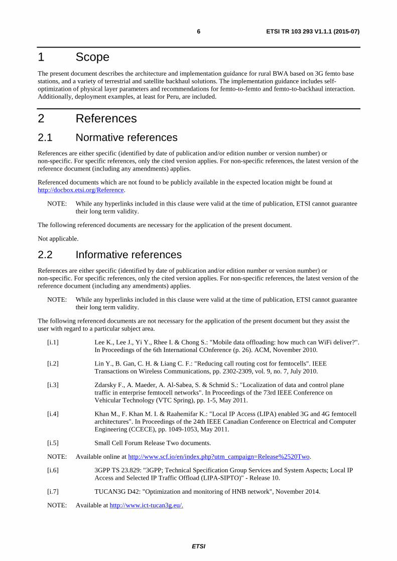
The PHY layer and the MAC layer establish limits in the coverage distance.

In PHY layer, the higher nominal bit rates are achieved with powerful modulations and low redundancy coding schemes, but it only works in short distances because the received power is high. So, the bit rate decreases with the distance. In point to point transmissions the transmitted power is the allowed maximum and the antenna gains are high. Figure 4.1 shows that long distances can be reached only if high gain directive antennas are used, i.e. 12 dB for omnidirectional antennas and 24 dBi for directional antennas.

Figure 4.1: Achievable distance for point to point, point to multipoint or mesh WiFi [i.9]

4.2.3 WiMAX (Worldwide Interoperability for Microwave Access)

The equipment based on IEEE 802.16 [i.18] standard is suitable to provide coverage to isolated areas with low cost and low time of deployment. The standard provides advantages like equipment interoperability, great robustness, higher security and the possibility to offer strict QoS support to all the communications in the network. It includes flexibility in the frequency bands (licensed and non-licensed) and in scenarios (fixed or mobile).

4.2.4 VSAT

The objective of the satellite links in rural BWA is to serve as IP transport network between gateways and the operator's network, mainly where the distance between gateways and operator's network is greater than 50 km. For broadband access and IP backhauling, and for the group of services where the cellular backhauling needed for remote rural can be considered into, it is accepted by industry that the best performance/cost solution for a satellite link is using a GEO (Geostationary Earth Orbit) satellite.

A geostationary orbit is a particular type of geosynchronous orbit. It is a circular orbit 35 786 km above the Earth's equator and following the direction of the Earth's rotation. A satellite in such an orbit has an orbital period equal to the Earth's rotational period (one sidereal day), and thus appears motionless, at a fixed position in the sky, to ground observers. The ground satellite antennas that communicate with the satellite do not have to move to track the satellite; they are pointed permanently at the position in the sky where the satellite stays.

While it is industry accepted that GEO satellites are the best option for fixed broadband access or IP backhauling, there are also recently industry developments and studies to offer these types of fixed services using MEO (Medium Earth Orbit) satellites.

MEO is the region of space around the Earth, located above LEO (Low Earth Orbit, altitude of 2 000 km) and below GEO (Geostationary Earth Orbit, altitude of 35 786 km). MEO satellites are widely used for navigation and geodetic/space environment science. The orbital periods of MEO satellites range from about 2 hours to nearly 24 hours. Examples of satellite systems in MEO for navigation are GPS (Global Positioning System) and Galileo.

As MEO satellites are not fixed in the sky frosingle ones and the system in composed of seIP backhaul, there is the need of using at leastvisible satellite, and a switchover of the commantenna is losing visibility of one satellite and

Using MEO satellites instead of GEO satellitereduced. IP communications trough a GEO sabe reduced four or five times (estimated RTTbackhauling GPRS/EDGE and 3G traffic, wh

Another difference between GEO and MEO ssatellites can provide full coverage to the Eartcovering 120º each one), while with MEO satupgraded to 12 satellites and 16 satellites.

Increase in cost of antenna subsystem to be abpointed to a GEO satellite, makes difficult to low traffic needs. They will be widely used fo

So for rural area deployments the best option satellite terminal will be cheaper.

4.3 Architecture exam

4.3.1 Overview

The architecture example has three main secti

• Access network (composed by femto

• Backhaul (an IP heterogeneous trans

• Network controller that manages the

These elements and the connection scheme ca

Figure 4

4.3.2 Network Controller

The Network Controller provides the followin

• Access Controller (AC) that aggreginterfaces (Iu-CS and Iu-PS) to the c

ETSI

ETSI TR 103 2912

from the point of view of a ground observer on Earth, thes several ones, and named constellation. If used for fixed brast two antennas with tracking devices. Each antenna movmmunications link from one antenna to the other is done pnd the other one is locked to the next satellite in the const

lites improve IP communications performance, as the dela satellite has an RTT of 600 ms to 650 ms, while with MET is 130 ms to 140 ms). This improvement is especially i

whose performance is very sensitive to delay in the transpo

satellite systems, for broadband access and backhauling,arth (but Poles) with only 3 satellites (if strategically deplsatellites are needed more. For example, O3b will start wit

able to track at least two MEO satellites, comparing to onto adopt this type of solutions for backhauling in very rem for backhauling between medium and big cities with high

on is to use a GEO satellite, as there will be more available

mple

ctions:

mtocells)

ansport network)

the cells and acts as gateway with the core network

can be seen in figure 4.2.

4.2: Network architecture example

wing functionality:

regates the traffic carried over IP from the femtocells and e core network.

293 V1.1.1 (2015-07)

ese satellites are not broadband access or oves and tracks one

e periodically as one nstellation.

elay is significantly EO satellites it can

y important when sport network.

ng, is that GEO ployed in the orbit, ith 8 satellites, to be

one single antenna emote areas with very igh demand of traffic.

ble satellites and the

provides standard

• IPsec Gateway that provides the capController.

• NOS (Network Orchestration Systwith all the features needed to succe

4.3.3 Access Network

The access network will be based on femtocetherefore suitable for rural communications dneed to be installed on waterproof cases with controller will be synchronized through sync

4.3.4 Satellite backhaul sc

A system architecture using the satellite back

Figure 4.3: Sch

In this figure the CRL server is a server from validated by the Femtocell and Network Cont(e.g. if a femtocell has been stolen, its certific

Depending on the final emplacement, omni anto the residential area. Rather than sectoring awhen needed, getting the chance to increase c

5 Optimization and

5.1 Introduction

5.1.1 Rural deployment sc

From the point of view of the access network,in figure 5.1:

• Small communities, are characterizecoverage/capacity requirements can tower at high positions (see figure 5.

ETSI

ETSI TR 103 2913

capability of securing the traffic between the femtocells an

ystem) that forms a complete 3G provisioning and managecessfully deploy and operate an IP Access femtocells syst

cells, which are inexpensive, energy efficient and self-orgs deployments. The femtocells will be used in outdoor scenith external antenna. The femtocells of the access network nc Over IP, using a NTP (Network Time Protocol) server f

scenario

ckhaul in Peru is presented in figure 4.3.

cheme of the satellite backhaul scenario

m which Certificate Revocation Lists (CRLs) may be accontroller Security Gateway in order to know whether each ficate can be revoked).

i antennas or directional/sectored antennas will be used to a single site, multiple femtocells will be preferred to incr

e coverage at the same time.

and monitoring of HNB network

scenarios for HNB

rk, the different rural scenarios are grouped into three cate

ized by low traffic generation and concentrated populationan be efficiently solved by installing one or two collocated 5.1, schema A).

293 V1.1.1 (2015-07)

and the Access

agement solution ystem.

rganized, and cenarios, so they will rk and the network er for that purpose.

ccessed. CRLs are ch can still be trusted

to provide coverage ncrease capacity

ork

ategories as presented

ion and ted HNBs in the same

ETSI

ETSI TR 103 293 V1.1.1 (2015-07) 14

• Medium communities (see figure 5.1, schema B). The traffic density is low-medium and the population is disperse, the access network deployment can be performed by the appropriate number of HNB in low position. In these scenarios, a low number of deployed HNB, together with a sufficient number of licensed carrier frequencies, allow operators to conveniently allocate carriers and guarantee inter-cell interference-free operation. As the traffic density grows, frequency planning is needed.

• In large communities (see figure 5.1, schema C), where there is a high traffic density with hot-spots, the combination of HNBs in high position and multiple HNBs in low positions seems the most adequate network access architecture.

Figure 5.1: Outdoor rural scenarios

The previous scenarios address the cases where HNBs are installed outdoors. In general, indoor UEs do not observe a significant degradation of the service because the usual building in the rural scenarios studied is based in wooden walls. However, medium and large communities could have some buildings with brick walls, like school, hospital, or town hall. This new element demands a single HNB to provide the large traffic demand of indoor users, see figure 5.2.

Figure 5.2: Indoor rural scenarios

5.1.2 Network self-configuration procedures

5.1.2.1 Bounding coverage

In clause 5.4.1 of TUCAN3G D42 [i.7] is proposed a technique to adjust the coverage area inside of buildings by exploiting measurement reports from UEs. The coverage area does not vary dynamically.

5.1.2.2 Detection of new neighbours

The topic of detection of new neighbours is considered in clause 5.4.2 of TUCAN3G D42 [i.7], and addresses scenarios in figure 5.1, schema B and figure 5.1, schema C. Whilst identification of the macro-cellular layer is of both physical engineering and practical coverage importance, the most important aspects of these are the iterative decode and detected set reporting because these are best aligned with the goal and allow discovery of new neighbours rather than validate or optimize ones already known to the network. Consequently, they combine to move the process of self-configuration forward.

Small Communities Medium Communities

Large Communities

A) B)

C)

5.1.2.3 Frequency and prima

Techniques addressed here refer to all scenari(FCAP) in small-cell networks are designed aconsists in assigning one (or more) frequencynetworks and as such, it has received considerchallenges in the design will be how to incorphow to render the algorithms dynamic and am

5.1.3 Long-term traffic-awa

The procedures considered in the present clauadapts to the long-term traffic demands, namedemand, the user association as a way of balarange expansion whereby, in contrast to the opilot signal, thus increasing/decreasing the co

It is important to remark that all procedures (snetwork to the long-term traffic demand. Whiexecuted in the time scale of minutes, the use(see figure 5.3). The total energy available dethe available power for the pilot signal and dausers depends on how they are scheduled in etraffic demand. Therefore, the user associatio

Figure 5.3

5.1.4 Criteria for switching

A strategy for dynamically switching on and otechnical scenario for small communities, seetwo BSs are co-located in the same telecomm

ETSI

ETSI TR 103 2915

mary scrambling code selection

arios. Different algorithms for the frequency and PSC assid and evaluated in clause 5.4.3 of TUCAN3G D42 [i.7]. Fcy-code pair to each base station, is a fundamental problemderable attention in traditional (macro legacy cell) networkorporate the operating conditions of the rural networks into amenable to distributed implementation.

ware self-optimization procedures

lause explain how to auto-tune the access network in such mely: procedures for switching on/off HNBs as function oalancing the load over neighbouring active HNBs, and finae on/off criterion, it addresses the modification of the powe coverage area of each HNB.

(see figure 5.3) are coupled among them in order to adaphile cell range expansion (CRE) or on/off procedures are ser association procedures will be executed in the second

depends on the battery level and the harvesting process, w data transmission. Nevertheless, the actual data service exn every frame, a procedure executed in the order of millisetion also will be influenced by actual bit rates provided by

5.3: Connection between procedures

ng on/off HNBs

d off BSs is presented in clause 5.1 of TUCAN3G D42 [i.see figure 5.1, schema A. The scenario under consideration

munication tower and share the same energy units (batter

293 V1.1.1 (2015-07)

ssignment problem . FCAP, which lem in cellular orks. The main into the design and

ch a way that it of the hourly traffic

inally dynamic cell-wer devoted to the

apt the access re expected to be

nd level time scale, , which translates on experienced by the iseconds, short-term by the scheduler.

i.7], tackling the ion is the one where tery and solar panels).

ETSI

ETSI TR 103 293 V1.1.1 (2015-07) 16

5.1.5 Dynamic cell range expansion

Clause 5.4 of TUCAN3G D42 [i.7] investigates a procedure for automating the power allocated for the pilot signal in scenarios with multiple HNBs, adequate for rural deployments in medium and large communities powered by a non-free source of energy.

6 Interoperability of access and transport network

6.1 General The short-term access network optimization deals with topics like channel state-aware packet scheduling, congestion and admission control. Nevertheless, all these topics also depend on the quality of the backhaul, demanding certain kind of coordination between transport network and the access network.

It should be noted that linear-like architecture of the transport network has higher probability to produce congestion in the links close to the backhaul GW especially when the traffic demand increases. In this respect, there are several investigations on different techniques aiming at the reduction of the backhaul load by means of traffic offloading and local cache for satellite links.

Figure 6.1: Network architectures considered in: left) Napo river and right) Balsapuerto

ETSI

ETSI TR 103 293 V1.1.1 (2015-07) 17

6.2 Traffic offloading Femtocells or Home Node B were originally conceived to improve 3G/4G indoor coverage for home subscribers. In that scenario, HNBs relay the traffic towards the core network using a private (typically xDSL) backhaul network.

In rural BWA, femtocells may be used to provide outdoor coverage. On the other hand, while classical macrocells or NBs (Node B) are connected to the core network using an optical fibre, HNBs may be connected to the core using a WiFi multihop network. In this configuration, the traffic load is expected to be greater than in the indoor configuration due to higher number of users, while the capacity is severely constrained than the original scenario due to use of limited WiFi. This problem is even more acute in deployments where the connection with the core network also includes a satellite segment. A solution to reduce the load of the backhaul network and avoid outages associated to overloads is to implement offloading techniques allowing smart routing of local traffic as given in [i.1].

6.3 Network architectures and benefits of traffic offloading The alternatives analysed in the present document are (see figure 6.2):

a) installing a gateway/proxy in the backhaul;

b) local switching of users served by the same HNB; and

c) shortest path.

In figure 6.2 UE1 is connected to UE2 and UE3 is connected to UE4. The purple route corresponds to alternative a) (installing a gateway/proxy in the backhaul); the yellow route corresponds to alternative b) (local switching of users served by the same HNB); and the green route corresponds to alternative c) (shortest path). Note that the yellow line connecting UE3 and UE4 through the core network is the conventional route targeted to shorten for a better usage of the backhaul.

Figure 6.2: Different alternatives for local offloading

Alternative a) consists in installing a gateway in the node that connects the backhaul to the core network, see [i.2] and [i.3]. This avoids sending local traffic to the core network, which is a good solution for deployments where the connection between the backhaul and the core is limited or expensive (for example, when it is implemented using a satellite link).

Alternative b) consists in connecting the users served directly by the same HNB as outlined in [i.4]. This option is appropriate to access to local data and to voice calls between close-by users.

Alternative c) consists in routing all local traffic through the backhaul network using the route with the shortest number of hops. Although it is difficult to implement in practice, this solution will serve as a benchmark to assess the benefits of implementing local switching.

ETSI

ETSI TR 103 293 V1.1.1 (2015-07) 18

The key aspects of the performance evaluation of each alternative are:

1) Network topology

2) Link configuration (terminals and effective throughput)

3) Traffic models

6.4 Implementations in 3GPP networks

6.4.1 Offloading implementations complying with the 3GPP standard

3GPP has standardized Local IP Access (LIPA) and Selected IP Traffic Offload (SIPTO) mechanisms since 3GPP Release 10, gradually adding more functionality. Recently, was carried out work within the Small Cell Forum to look at enterprise data and offload architectures. Some of the results are available in reference [i.5]. These include the introduction of intermediate gateways for data and voice offloading, and mobility with reduced signalling towards the core network.

LIPA was designed as a service to allow a radio bearer access through a specific local IP address that is not publicly accessible – e.g. it is not on the public internet. The original use cases include access to enterprise intranets, home media storage, as well as printers (see 3GPP TS 23.829 [i.6]). SIPTO is a similar offloading optimization allowing a radio bearer towards a public address to be offloaded without traversing the operator core network, unlike LIPA.

In the case of rural deployment scenarios, the backhaul transportation to the Core Network is expected to have a high latency in addition to existing limited bandwidth problem which probably causes multiple congestions due to the deployment conditions. Consequently, it is highly beneficial to use a technology to reduce the load (either signalling or user data) on the backhaul. The expected growth of the population of the communities may entail a significant increase of the local traffic, including voice (VoIP). The reference architectures will take advantage of this. Such techniques may also improve the user experience.

6.4.2 Non-standard offloading implementations: data traffic caching over satellite

6.4.2.1 Introduction

In addition to the ones in 3GPP standards, there are pre-standard or non-standard implementations, including some on the border of content delivery, that provide alternative offload mechanisms. When analysed in detail, it can be seen that some of the mechanisms are simpler to implement and adapt to the specific scenarios considered. Although such techniques may provide considerable benefits to the user experience, some of the proposed implementations will also have disadvantages in terms of reliability, flexibility, modifications to existing protocols, security, and exposure of the internal structure of the core network (e.g. IP addresses usage).

Internet content keeps expanding rapidly with richer contents and web sites which include more and more visual materials – static and motion based. Nowadays, most visited web pages are larger than ever. In addition, Web sites become very dynamic with content preloading every time the user moves their cursor over an object or link. On the other hand, home and business networks have far more networking devices than ever, with laptops, tablets, smartphones and many other devices connecting via 3G networks or WiFi.

This explosion of Internet contents makes the access through VSAT really challenging. Throughout the past decade, VSAT equipment manufacturers were able to improve web performance using various web acceleration technologies:

• Content cache: Onboard cache memory for recently or frequently accessed documents, objects or scripts and pre-fetch documents that are likely to be accessed, DNS caching.

• HTTP Compression: Use of encoding methods.

• Code Optimization: Optimizing java or http code to send the less information possible, this feature includes "White Space Removal" and "compressing images"

Among the three, only the first requires additional network elements and is relevant to the proposed rural BWA architecture.

ETSI

ETSI TR 103 293 V1.1.1 (2015-07) 19

Although traditional hierarchical web cache control technologies provide tremendous improvement in web user experience, satellite-cache distribution technologies could extremely improve the results. This progress can be obtained by utilizing a large on-board multi Gigabyte memory in the central cache. This way, a large amount of web content could be stored and by taking advantage of the inherent one-to-many satellite network topology, to distribute and populate content on the cache memory of all VSATs in a particular network.

Each object in a web page has a date of expiration which is used by cache devices to understand if the object can be saved and how long. The use of cache devices reduces the number of requests by providing memory local cache, previously captured data and by improving the response times (in average) and the use of bandwidth.

6.4.2.2 Content caching

Caching is not new to Internet technology. Caching technology like other acceleration methods is designed to reduce bandwidth and enhance the user experience. The main idea of content caching is to store popular content which is frequently accessed by the users. Whenever a user desires to access the required content, the content is fetched immediately from the local cache storage instead of fetching it from the remote web server.

Today cache servers are deployed throughout the Internet at either the core (carriers), the edge Internet Service Providers (ISPs) or the end user locations. Caching is also available on web browsers. In low roundtrip delay networks, the combined use of caching by the ISP and caching at the browser will provide enough performance improvement to end users. However, when ISPs and end users are separated by an around 600 ms of round trip delay and an expensive transmission path (space segment), the performance improvement is diminished.

Figure 6.3: Web Cache-Architecture

As shown in figure 6.3, cache servers at the hub location are typically installed by satellite ISPs in order to reduce the terrestrial backhaul usage and to bring content closer to the user. Nevertheless, the traffic still needs to travel more than 72 000 km between the hub and the end user. The objective of satellite cache technology is to bring the content within a shorter distance (hence with lower delays) to the end users based on Distributed Cache architecture located at every site in the network. In this architecture each cache stores the content that has been accessed by local users and then common content is also shared with all other cache elements in the network. As a result each cache device contains all of the content that has been accessed by any user in the network. This architecture is mostly suitable for VSAT networks because of the inherent one-to-many broadcast characteristics of satellite. Content needs to be transmitted only once over the satellite to be received and stored by each of the satellite network nodes.

ETSI

ETSI TR 103 293 V1.1.1 (2015-07) 20

6.4.2.3 Content caching tests in Peru

In February 2013, a 5-days test of internet traffic download was carried out. Optimization was done using web caching features on VSAT modems. During the tests, Web Enhance VSAT is used for distributed caching, and Skymon software is used to measure the traffic offloading optimization. The main focus of the analysis was the satellite bandwidth optimization, as well as the improvement of the user experience with faster downloads. The tests were performed in two different scenarios:

• Controlled environment with one VSAT

• Multiple VSATs

6.4.2.4 One VSAT working in a controlled environment

The purpose of this experiment is to test VSAT cache capability directly and under controlled conditions. The simplified architecture of the test environment is given in figure 6.4, where there is one VSAT placed in the lab and two computers connected to the VSAT.

Figure 6.4: Simplified architecture for the experiments with one VSAT

A brief list of webpages is selected for the tests, and then they opened in PC1. Since the VSAT cache was empty at the beginning, all the page details had to be downloaded entirely through the outbound. The next step consisted to access the same list of pages, but this time from the PC2. In this case, many of the objects of those pages were downloaded directly from the VSAT cache.

Figure 6.4 depicts an example of the Outbound traffic associated to the VSAT. This figure includes both downloads, from the PC1 (all pages and items are served entirely in the Outbound), and from the PC2. In the left side of figure 6.5 the outbound traffic is displayed during the time all pages are downloaded from the PC1, while the right side of figure 6.5 shows the outbound traffic during the download from the PC2 (using the VSAT cache). As expected, the outbound traffic for the PC2 is relatively lower and VSAT caching succeeded to reduce in more than 20 % the outbound usage.

ETSI

ETSI TR 103 293 V1.1.1 (2015-07) 21

Figure 6.5: Outbound graph associated to the VSAT

On the other hand, the download time for both situations has been evaluated and is given in table 6.1. The first column shows the selection of the web pages used during the tests, while the second and the third column show download durations for the attempts from PC1 and PC2 respectively. Except for a couple of particular cases, the second attempt has a lower download time.

Table 6.1: Website download time comparison (in seconds)

URL list Attempt 1 Attempt 2

17:30 18:30 http://www.hotmail.com 18,281 11,843 http://www.hi5.com 17,398 15,125 http://www.rpp.com.pe 31,109 26,226 http://www.elcomercioperu.com.pe 25,046 13,781 http://www.youtube.com 6,257 6,765 http://www.wikipedia.org 5,179 2,015 http://www.facebook.com 17,953 9,304 http://www.sunat.gob.pe 15,609 25,757 http://www.peru21.pe 37,968 18,039 http://www.claro.com.pe 40 40 http://www.viabcp.com 0,023 0,007

6.4.2.5 Multiple VSATs

In the configuration shown in figure 6.6, nine operational VSAT are installed in Internet cafes. The objective of this second phase consists of determining the outbound savings for long term traffic by adding the cache capability of representative sites while they work all day long. This will give a good indication of quantitative values associated to total bandwidth saving on the outbound if it is assumed to have similar traffic pattern and similar number of computers in most of the VSAT locations.

http://www.hotmail.com/

http://www.hi5.com/

http://www.rpp.com.pe/

http://www.elcomercioperu.com.pe/

http://www.youtube.com/

http://www.wikipedia.org/

http://www.facebook.com/

http://www.sunat.gob.pe/

http://www.peru21.pe/

http://www.claro.com.pe/

http://www.viabcp.com/

ETSI

ETSI TR 103 293 V1.1.1 (2015-07) 22

Figure 6.6: Architecture for the experiments with multiple VSAT

Specific graphics directly associated to the Web Enhance capabilities are used. These graphs represent the traffic volume that would have been transmitted by the outbound, if there were no cache in the VSAT, versus the traffic volume that is actually transmitted over satellite.

In figure 6.7 is represented the traffic served from cache relative to the total traffic during one day, while in figure 6.8 is represented the traffic served from cache relative to the total traffic during seven days.

Figure 6.7: HTTP traffic in one day

ETSI

ETSI TR 103 293 V1.1.1 (2015-07) 23

Figure 6.8: HTTP traffic in 7 days

From figure 6.7 and figure 6.8 results:

• Cache-based solution saves 15 % to 20 % of required traffic volume.

• In the busy hours, those savings are up to 40 %, which corresponds to 1 Mbit/s to 2 Mbit/s for the nine sites.

6.5 Access network and backhaul interplay

6.5.1 3GPP background

The QoS architecture for 3GPP mobile networks is described in ETSI TS 123 207 [i.14]. Furthermore, in ETSI TS 123 207 [i.14] the architecture is extended to provide end-to-end QoS. Specifically, when resources not owned or controlled by the UMTS network are involved in the UMTS data transport, it is necessary to interwork with the network that controls those resources. ETSI TS 123 207 [i.14] defines several approaches for this interaction:

a) signalling along the flow path (e.g. RSVP) and packet marking or labelling along the flow path (e.g. DiffServ or MPLS). According to ETSI TS 123 207 [i.14], both the GGSN and the UE should support DiffServ edge functionalities, but RSVP support is optional;

b) interactions between both network management elements; and

c) service level agreements.

The annex A of the ETSI TS 123 207 [i.14] describes different scenarios of 3GPP networks that include a non-3GPP backbone network. These scenarios correspond to different UE and GGSN capabilities. In all the cases, the non-3GPP network is in the core network and the AN is supposed to be UMTS-controlled. Then, the QoS in the AN is simply managed by the PDP Context signalling. The solutions for these scenarios comprise the combination of DSCP marking and RSVP with application layer signalling (mainly SIP and SDP).

In addition, the nature of the security model used is important as impacts whether and how an AP can receive or derive information about the state of the backhaul and different approaches may be needed. The two possible scenarios are:

1) Traditional Secure Deployment. The default Iuh reference model is as shown in figure 6.9. The default security model for standard deployments provides end-to-end security with the user and control planes protected by an IPSec tunnel, and the management traffic to the HMS is also using the same or a different secure link. A HNB will not generally accept messages from a non-trusted source. Consequently, in this case the ability to monitor the state of the backhaul will be dependent on what the HNB can derive from the incoming traffic by itself, or indicators supplied by a trusted source, e.g. down the IPSec tunnel, or from an intermediate node via an additional secure link with a chain of trust.

Figure 6.9: D

2) Non-secure deployment. In this scenuser data and possible for control sigdemand on the backhaul, enabling eastate and potentially allowing some rnot considered for the rural scenario

In rural scenario the non-3GPP network is planot directly applicable. Moreover, as it is discsupported by most of the equipment typicallyneeded in order that the AN can collect the BHHence, a different non-standard solution shou

6.5.2 Structure of the AN-

Figure 6.10 shows the architecture of the comHNB-gateway. The ABI is placed between thpresent document is the part of the network beis the part that goes from the gateway to the Harrows represent data or signalling exchange abetween the AN and the BH are provided by t

Figure 6.10: Network

Below is presented an overview of the ABI pr

1) The AN requires BH state informatiodecisions. The required information,defined in TUCAN3G D51 [i.10] an

2) The AN requires that the BH guaran

3) A joint optimization algorithm may power, modulation and coding schemfor the AN being able to modify BH

ETSI

ETSI TR 103 2924

Default Iuh reference model (see [i.13])

enario there is no secure link from the HNB to the HNB-Gsignalling as well. This has advantages like reducing the o easier communication of any external messages looking ae routing optimization. However, by definition, it is not se

rio.

placed between the core network and the HNB, and henceiscussed in TUCAN3G D51 [i.10], the IntServ option withlly used in wireless backhauls. Finally, additional function BH-state to perform backhaul-aware admission control anould be designed for rural BWA access, which is outlined

-BH interface

omplete network that implements the Iuh interface, from th the edge routers and the HNBs, and the wireless BH consbetween the ABI and the gateway. Another part of the BH

e HNB-GW. Figure 6.10 represents the structure of the ABe and slashed thin arrows represent logical interactions. Fy the ABI, which are:

ork architecture: access network and backhaul

I procedures.

ation in order to make appropriate BH-aware scheduling on, its accuracy and the updating frequency have been and are summarized in continuation.

rantees a certain QoS level for each type of traffic flow.

ay need to dynamically configure BH nodes' parameters (liheme or routing). In this case, the ABI should provide a coH behaviour. Alternatives are briefly discussed in TUCA

293 V1.1.1 (2015-07)

GW deployed for e overall data rate g at the backhaul t secure, and then is

ce these solutions are ith RSVP is not

ionalities would be l and scheduling. ed in clause 6.5.2.

the HNBs to the nsidered in the BH (possibly wired) ABI. Solid thick . Four interactions

(like transmission control mechanism AN3G D51 [i.10].

4) Regarding the exchange of traffic daEthernet cable), and the gateway rouHNB and the HNB-GW is implemenis done in the IP level.

The main AN-BH interactions are shown in fi

Figure 6.11: AN to

Finally, any solution should also take into accHNB may be able to limit the amount of trafftrack of the traffic inserted into each downlinkBH is carried out between the HNB and the e

6.5.3 Information requirem

Backhaul aware admission control and packetthat are known by the HNB. First, admission information, like available rate, current delay network topology. Second, the state informatiinformation can be collected for individual lindependent or aggregated.

Mainly four parameters are needed: availablelevel. For the offloading algorithms, also topo

Normal functioning of 3GPP signalling proceadmission control procedure needs to request upper bound on the response time is needed. Arequired from the BH could be high. Then, it shows the requirements for both procedures. Tneeded is really short and the periodicity betwAN request and a subsequent BH response is should be very frequently updated in the HNB

ETSI

ETSI TR 103 2925

data, an edge router is placed back to back to each HNB (router is placed in the other end of the BH. The Iuh interfa

ented as an IP tunnel. Hence, the data exchange between

figure 6.11.

to BH interface (ABI) with main interactions

account the different limitations on the UL and DL implemaffic it inserts in to the uplink, a HNB-GW does not have tlink towards an HNB. Hence, the main interaction betweene edge router.

ement for AN algorithms

ket scheduling algorithms will depend on the available BHn control and scheduling procedures may need different ty

ay and jitter, congestion level, status of the BH nodes' battation may be needed with a different frequency and accur links or for end-to-end path, and part of the information m

le rate of the BH, delay, the queues length of the BH-nodepology knowledge would be useful.

cedures imposes certain constraints to the ABI design. Foest instantaneous BH-state information from the backhaul,d. Also, if a procedure is executed very frequently, the amo it is necessary to characterize the requirements for each ps. The time between a procedure starts and the BH state inetween scheduling procedures is only 2 ms. Hence, a proce is not suitable, since it would imply a higher latency. ThenNB.

293 V1.1.1 (2015-07)

B (with a gigabit rface between the en the AN and the BH

lementation: whilst an e the resource to keep een the AN and the

BH-state parameters t types of atteries, or even the uracy. Third, the

n may be flow

odes and battery

For example, if the ul, a very stringent mount of information procedure. Table 6.2 information is ocedure based on an hen, the information

ETSI

ETSI TR 103 293 V1.1.1 (2015-07) 26

Table 6.2: Access network algorithms requirements

Procedure Maximum latency Periodicity BH aware admission

control algorithm Very low in order to avoid latency in call

setup (in order of a few milliseconds)

Once for each connection: several times per minute

BH aware packet scheduling

Much lower than frame duration: << 2 ms

One for each frame: 2 ms

7 Backhaul aware scheduling

7.1 Backhaul-aware scheduling with a single HNB

7.1.1 Overview

Users demanding a fixed service rate (voice users) are prioritized over users that request a flexible service rate (data users). Therefore, the average throughput achieved by the data users will depend on the available resources as well as on the random channels experienced by the users. When there is no reason for treating flexible service rate users differently, proportional fair (PF) is a meaningful scheduling approach. The reason for that is well-known: PF aims to achieve long-term fairness among users while taking advantage of the fact that a specific user has a momentary good channel. This is achieved by maximizing, at each scheduling period, a weighted sum-rate where each weight, updated after each scheduling period, keeps memory of the throughput already served to the corresponding user to enforce fairness. Backhaul capacity limitation can be introduced in the proportional fair scheduler by imposing an instantaneous aggregate traffic rate constraint according the backhaul capacity. Instantaneous aggregate traffic rate limitation to model the limit backhaul capacity has been considered in ETSI TS 133 320 [i.16].

However, backhaul capacity can be measured in average terms only. Limiting the instantaneous sum-rate at each specific scheduling period according to such average value may hamper the performance of the system in terms of the achievable long-term rates. In these circumstances, it seems less limiting using high data rates in the air interface whenever the channel conditions allow (even to a greater value of that imposed by the average backhaul constraint) provided that the backhaul constraint is met when averaging the traffic served in several scheduling periods. However, how to introduce this long-term backhaul constraint within the proportional fair scheduler formulation is not straightforward.

In the present document is proposed a long term hard fairness scheduler with a long-term backhaul constraint. The goal is, as for the proportional fair approach, to provide an equal long-term rate to a set of data users, guaranteeing the service to the voice users. Different from the PF, are used stochastic optimization tools to maximize the long-term achievable rate according to the wireless channel statistics and the maximum backhaul capacity. The algorithm decides the long-term rates to be allocated to the users. Then, based on the long-term decision rate decision, at each scheduling period a concrete resource allocation is decided based on the user specific channel conditions and the long-term rate goal. One additional advantage of this algorithm is that it allows to obtaining accurate information regarding the impact of each user on the maximum achievable long-term rate of all the users. This information can be useful to stablish admission policies in case the achievable long-term rate is unacceptable low.

Along with the limited backhaul capacity, another distinctive feature of rural BWA scenarios is the fact that BSs are powered with solar panels batteries of reduced size. Because of that, the energy available at the BS is a limited resource as well and the average throughput achieved by the data users will be certainly impacted by this limitation. For such a reason, the performance of the schedulers is optimized subject to the energy limitations that depend on the battery status and on the harvesting capabilities, e.g. solar panels used to recharge the battery.

7.1.2 Downlink scheduling

7.1.2.1 System description and assumptions

In this clause is considered the downlink (DL) of a WCDMA system. Given a power budget for the HNB, the goal is to optimize the number of codes and the power allocated to each user to maximize the data throughputs, while guaranteeing the voice service.

ETSI

ETSI TR 103 293 V1.1.1 (2015-07) 27

To address the problem is considered that a set of voice users, KV, and a set of data users, KD, are already admitted in the system. In case that a certain user has a data connection and a voice connection simultaneously, such a user will be treated as two independent users, one for each connection.

Whatever the scheduling strategy is, the radio resources that can be distributed among users at each scheduling period in the air interface are the number of codes and/or power. It is considered that each voice user is assigned one dedicated physical channel from a pool of NV voice channels (each one consisting in a code of, for instance, a spreading factor (SF) of 128).

If the data channels and the dedicated channels for voice use the same carrier, the power of the carrier and the code tree is shared between both types of channels. Usually the number of available codes with greater SF depends on how many codes with shorter SF are used. To guarantee that codes with greater SF are available, i.e. voice codes, a limitation can be imposed on the number of available codes with shorter SF, i.e. data codes. In HSDPA the maximum number of HS-DPSCH codes, i.e. the physical channels used for data transmission, is less than or equal to 15, even if there are up to 16 possible codes. Additionally, if the power of the carrier is shared among data and voice channels, there is a common constraint in the HNB power.

It is important to mention that in practice, when HSDPA is considered instead of Release 99, variable SF and fast power control are disabled and replaced by adaptive modulation and coding (AMC) and extensive multi-code operation. The idea in HSDPA is to enable a scheduling such that, if desired, most of the cell capacity may be allocated to one user for a very short time, when channel conditions are favourable. The total number of channelization codes with SF 16 is respectively 16 (under the same scrambling code). In the code domain perspective, the SF is fixed; it is always 16, and multi-code transmission as well as code multiplexing of different users can take place. The maximum number of codes that can be allocated is 15, but depending on the terminal capability, individual terminals may receive a maximum of 5 codes, 10 codes or 15 codes. The Transmission Time Interval (TTI) or interleaving period has been defined to be 2 ms which is shorter compared with the 10 ms, 20 ms, 40 ms or 80 ms TTI sizes supported in Release 99.

7.1.2.2 Simulation results

In this clause are presented the numerical results for the backhaul and channel aware stochastic scheduler and the PF scheduler. The scenario under consideration in this clause is composed of one base station, 3 voice users and 6 data users. The maximum radiated power of the BS is 13 dBm and includes the pilot power of 4 dBm (which represents the 13 % of the maximum radiated power, and the power the BS can use for voice and data users. In addition to the radiated power, the BS spends a fixed power of 3 dBm.

The number of available codes for data transmission services is 15. All the users are mobile with a speed of 3 m/s. The instantaneous channel incorporates antenna gains, Rayleigh fading with unitary power, and a real path loss of San Juan village in Peru. The orthogonality factor is 0,35. The code gain of data codes is 16 and the minimum SINR normalized with code gain for voice users is -13,7 dB which corresponds to a rate of 12,2 kbit/s. The noise power is -102 dBm. The battery maximum capacity is 410 µJ, the energy provided from solar panels is assumed 30 µJ (Hi(t) in equation (3), section A.3). The scheduling period for the data users and voice users are 2 ms and 20 ms, respectively.

Two values for the total backhaul capacity have been considered in the simulations: 2 Mbit/s and 500 kbit/s. The amount of backhaul capacity required by the 3 voice users considered in this deployment is 173 kbit/s. The overhead for the data transmissions is 1,2.

Note that the stochastic scheduling strategy cannot be compared directly in a fair way with the PF approach under a sum-rate constraint. The reason is because the backhaul capacity was divided equally among users in average terms, whereas in the PF with sum-rate constraint, the overall backhaul capacity is not forced to be distributed equally.

Figure 7.1 shows the time evolution of the expected data rates of the three approaches. The backhaul capacity is 2 Mbit/s. Initially, it is assumes that the queues at the access network are sufficiently full so that all the bits demanded by the users are served. This makes the initial average rates violate the backhaul capacity constraint for a short period of time (see the initial transient in figure 7.1). When the average rates converge, they fulfil all the constraints of the original problem. As can be seen from figure 7.1, the limitation of the rates comes from the limited resources available at the access network, i.e. the power and the codes, as the backhaul capacity is not reached. It should be also emphasized that, the proposed stochastic approach provides a solution that introduces more fairness when compared with the PF approach as the average rates for the different users are quite similar.

ETSI

ETSI TR 103 293 V1.1.1 (2015-07) 28

Figure 7.1: Average data rates for different schedulers for a total backhaul capacity of 2 Mbit/s

Figure 7.2 depicts the sum of the average data rates as a function of the total overall backhaul capacity for the different approaches when the BS is connected to the grid and when the BS has a finite battery with different harvesting intensities p. The black dashed line shows the total available backhaul for data users. In figure 7.2, is possible to identify when the system is limited by backhaul and when the system is limited by the access network. For example, for the stochastic case connected to the grid, the system is limited by the access network when the capacity of the backhaul is above 1,2 Mbit/s.

Figure 7.2: Sum-rate served in the air interface for data users versus the total backhaul capacity

7.1.3 Uplink scheduling

7.1.3.1 System description and assumptions

Similarly to the work done for the DL, allocation of codes and power to each active user will be considered in this clause for the uplink (UL). The main difference is that now there is a power budget constraint per user, not per HNB.

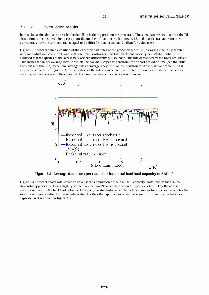
ETSI

ETSI TR 103 293 V1.1.1 (2015-07) 29

7.1.3.2 Simulation results

In this clause the simulation results for the UL scheduling problem are presented. The same parameters taken for the DL simulations are considered here, except for the number of data codes that now is 13, and that the transmission power corresponds now the terminal and is equal to 24 dBm for data users and 21 dBm for voice users.

Figure 7.3 shows the time evolution of the expected data rates of the proposed scheduler, as well as the PF scheduler with individual rate constraints and with total rate constraints. The total backhaul capacity is 2 Mbit/s. Initially is assumed that the queues at the access network are sufficiently full so that all the bits demanded by the users are served. This makes the initial average rates to violate the backhaul capacity constraint for a short period of time (see the initial transient in figure 7.3). When the average rates converge, they fulfil all the constraints of the original problem. As it may be observed from figure 7.3, the limitation of the rates comes from the limited resources available at the access network, i.e. the power and the codes. In this case, the backhaul capacity is not reached.

Figure 7.3: Average data rates per data user for a total backhaul capacity of 2 Mbit/s

Figure 7.4 shows the total rate served to data users as a function of the backhaul capacity. Note that, in the UL, the stochastic approach performs slightly worse than the two PF schedulers when the system is limited by the access network and not by the backhaul network. However, the stochastic scheduler offers a greater fairness, so the rate for the worst case users is better for the scheduler than for the other approaches when the system is limited by the backhaul capacity, as it is shown in figure 7.5.

ETSI

ETSI TR 103 293 V1.1.1 (2015-07) 30

Figure 7.4: Sum-rate served in the air interface for data users versus the total backhaul capacity

Figure 7.5: Rate served in the air interface for the worst case data user versus the total backhaul capacity

7.2 Backhaul aware scheduling with multiple HNBs

7.2.1 Overview

In this clause, the focus is on designing dynamic resource allocation schemes (both for uplink and downlink) that take into account the fact that multiple HNBs are present. This implies that users of different cells will be jointly optimized (in contrast with the previous case, where the optimization was carried out only for users within the same cell). Main points to be considered in the updated design are:

a) The objective now needs to consider all users and HNBs jointly. This can be achieved by using a multi-objective optimization approach or just by redefining the objective as weighted sum of individual objectives.

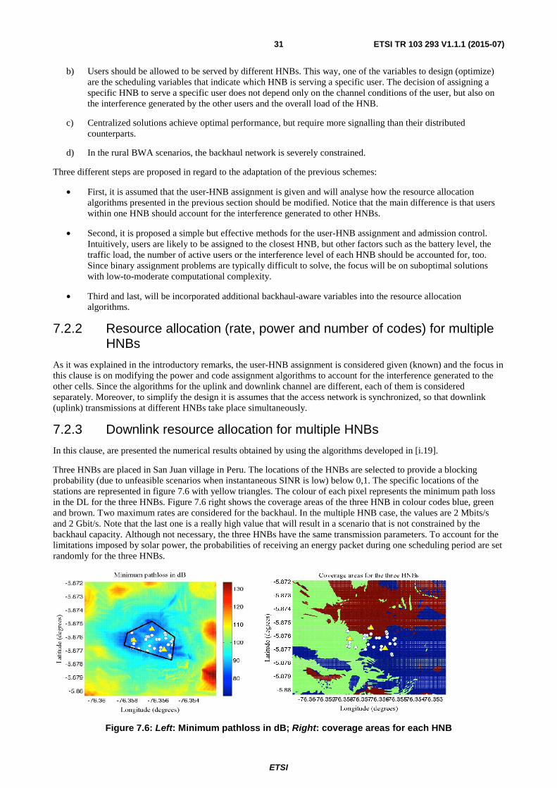
ETSI

ETSI TR 103 293 V1.1.1 (2015-07) 31

b) Users should be allowed to be served by different HNBs. This way, one of the variables to design (optimize) are the scheduling variables that indicate which HNB is serving a specific user. The decision of assigning a specific HNB to serve a specific user does not depend only on the channel conditions of the user, but also on the interference generated by the other users and the overall load of the HNB.

c) Centralized solutions achieve optimal performance, but require more signalling than their distributed counterparts.

d) In the rural BWA scenarios, the backhaul network is severely constrained.

Three different steps are proposed in regard to the adaptation of the previous schemes:

• First, it is assumed that the user-HNB assignment is given and will analyse how the resource allocation algorithms presented in the previous section should be modified. Notice that the main difference is that users within one HNB should account for the interference generated to other HNBs.

• Second, it is proposed a simple but effective methods for the user-HNB assignment and admission control. Intuitively, users are likely to be assigned to the closest HNB, but other factors such as the battery level, the traffic load, the number of active users or the interference level of each HNB should be accounted for, too. Since binary assignment problems are typically difficult to solve, the focus will be on suboptimal solutions with low-to-moderate computational complexity.

• Third and last, will be incorporated additional backhaul-aware variables into the resource allocation algorithms.

7.2.2 Resource allocation (rate, power and number of codes) for multiple HNBs

As it was explained in the introductory remarks, the user-HNB assignment is considered given (known) and the focus in this clause is on modifying the power and code assignment algorithms to account for the interference generated to the other cells. Since the algorithms for the uplink and downlink channel are different, each of them is considered separately. Moreover, to simplify the design it is assumes that the access network is synchronized, so that downlink (uplink) transmissions at different HNBs take place simultaneously.

7.2.3 Downlink resource allocation for multiple HNBs

In this clause, are presented the numerical results obtained by using the algorithms developed in [i.19].

Three HNBs are placed in San Juan village in Peru. The locations of the HNBs are selected to provide a blocking probability (due to unfeasible scenarios when instantaneous SINR is low) below 0,1. The specific locations of the stations are represented in figure 7.6 with yellow triangles. The colour of each pixel represents the minimum path loss in the DL for the three HNBs. Figure 7.6 right shows the coverage areas of the three HNB in colour codes blue, green and brown. Two maximum rates are considered for the backhaul. In the multiple HNB case, the values are 2 Mbits/s and 2 Gbit/s. Note that the last one is a really high value that will result in a scenario that is not constrained by the backhaul capacity. Although not necessary, the three HNBs have the same transmission parameters. To account for the limitations imposed by solar power, the probabilities of receiving an energy packet during one scheduling period are set randomly for the three HNBs.

Figure 7.6: Left: Minimum pathloss in dB; Right: coverage areas for each HNB

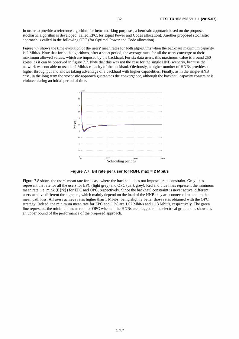
ETSI

ETSI TR 103 293 V1.1.1 (2015-07) 32

In order to provide a reference algorithm for benchmarking purposes, a heuristic approach based on the proposed stochastic algorithm is developed (called EPC, for Equal Power and Codes allocation). Another proposed stochastic approach is called in the following OPC (for Optimal Power and Code allocation).

Figure 7.7 shows the time evolution of the users' mean rates for both algorithms when the backhaul maximum capacity is 2 Mbit/s. Note that for both algorithms, after a short period, the average rates for all the users converge to their maximum allowed values, which are imposed by the backhaul. For six data users, this maximum value is around 250 kbit/s, as it can be observed in figure 7.7. Note that this was not the case for the single HNB scenario, because the network was not able to use the 2 Mbit/s capacity of the backhaul. Obviously, a higher number of HNBs provides a higher throughput and allows taking advantage of a backhaul with higher capabilities. Finally, as in the single-HNB case, in the long term the stochastic approach guarantees the convergence, although the backhaul capacity constraint is violated during an initial period of time.

Figure 7.7: Bit rate per user for RBH, max = 2 Mbit/s

Figure 7.8 shows the users' mean rate for a case where the backhaul does not impose a rate constraint. Grey lines represent the rate for all the users for EPC (light grey) and OPC (dark grey). Red and blue lines represent the minimum mean rate, i.e. mink (E{rk}) for EPC and OPC, respectively. Since the backhaul constraint is never active, different users achieve different throughputs, which mainly depend on the load of the HNB they are connected to, and on the mean path loss. All users achieve rates higher than 1 Mbit/s, being slightly better those rates obtained with the OPC strategy. Indeed, the minimum mean rate for EPC and OPC are 1,07 Mbit/s and 1,13 Mbit/s, respectively. The green line represents the minimum mean rate for OPC when all the HNBs are plugged to the electrical grid, and is shown as an upper bound of the performance of the proposed approach.

0 5000 10000 150000

0.5

1

1.5

2

2.5

3

3.5

4

4.5

5x 10

5

Scheduling periods

bits

/s

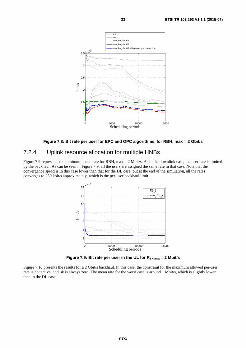
ETSI

ETSI TR 103 293 V1.1.1 (2015-07) 33

Figure 7.8: Bit rate per user for EPC and OPC algorithms, for RBH, max = 2 Gbit/s

7.2.4 Uplink resource allocation for multiple HNBs

Figure 7.9 represents the minimum mean rate for RBH, max = 2 Mbit/s. As in the downlink case, the user rate is limited by the backhaul. As can be seen in Figure 7.9, all the users are assigned the same rate in that case. Note that the convergence speed is in this case lower than that for the DL case, but at the end of the simulation, all the rates converges to 250 kbit/s approximately, which is the per-user backhaul limit.

Figure 7.9: Bit rate per user in the UL for RBH,max = 2 Mbit/s

Figure 7.10 presents the results for a 2 Gbit/s backhaul. In this case, the constraint for the maximum allowed per-user rate is not active, and μk is always zero. The mean rate for the worst case is around 1 Mbit/s, which is slightly lower than in the DL case.

0 5000 10000 15000

1

1.5

2

2.5

3

3.5x 10

6

Scheduling periods

bits

/s

EPOPmin

k E{r

k} for EP

mink E{r

k} for OP

mink E{r

k} for OP with power grid connection

0 5000 10000 15000

2

4

6

8

10

12

14x 10

5

Scheduling periods

bits

/s

E{rk}

mink E{r

k}

ETSI

ETSI TR 103 293 V1.1.1 (2015-07) 34

Figure 7.10: Bit rate per user in the UL for RBH,max = 2 Gbit/s

7.3 Congestion Detection and Measurement

7.3.1 Introduction

It is useful to consider the impact of congestion on the performance of the system. The impact is principally noticeable on real time audio and video services, using Real time Protocol (RTP), because packet-based applications have historically been designed to be more sensitive to delay, and any congestion management procedures need to assess the overall impact on the system performance and user experience.

7.3.2 Analysis of a deployment case

7.3.2.1 Delay

The relevant RTP performance related indicators are mean and maximum hourly statistics, reported separately for CS (Circuit Switched) and PS (Packet Switched) services:

• UL/DL Jitter (maximum and mean)

• UL/DL Packet Loss (maximum and mean)

• Round Trip Transmission Delay (RTT) (maximum and mean)

The HNB and HNB-GW employ jitter buffers to tackle inter-packet delay variance and therefore call quality can be estimated by overall delay time and packet loss generated by the backhaul network.

The Recommendation ITU-T G.114 [i.11] states "one way, end-to-end transmission time" constraints:

• 0 ms to 150 ms: Acceptable for most user applications;

• 150 ms to 400 ms: Acceptable provided that Administrations are aware of the transmission time impact on the transmission quality of user applications;

• Greater than 400 ms: Unacceptable for general network planning purposes.

Although these thresholds are general ones and it is noted in Recommendation ITU-T G.114 [i.11] that some delay-sensitive applications may require delays less than 150 ms and, on other hand, delays greater than 400 ms are acceptable in certain special cases (satellite links for example), these thresholds are good reference points.

It was found that:

• Averaged Maximum UL/DL CS Jitter has 91st percentile below 150 ms and 97th to 99th percentile below 400 ms.

• Averaged Maximum CS RTT Delay is 88 % below 150 ms and 95 % below 400 ms.

0 5000 10000 15000

0.5

1

1.5

2

2.5

3x 10

6

Scheduling periods

bits

/s

E{rk}

mink E{r

k}

Figure

In figure 7.11, the UL/DL maximum jitter anddata) it is shown distributed over millisecond

7.3.2.2 Frame loss

The 3GPP Technical Report TR 25.853 [i.12for real time audio and less than 1 % for real t

In the analysed data set it was found that CS p

In uplink:

• 84,92 % of reports contain packet lo

• 94,7 % below 0,1 %

• 99 % below 1 %

• 99,9 % below 5 %

In downlink:

• 19,1 % of reports contain packet loss

• 80,6 % below 0,1 %

• 96,7 % below 1 %

• 99,4 % below 5 %

ETSI

ETSI TR 103 2935

re 7.11: Jitter and RTT histograms

and the round trip delay time (RTT) per DSCP code (46 isnd ranges.

12] on access stratum delay specifies end-to-end frame losal time video services.

S packet loss figures are as follows:

loss equal 0

loss equal 0

293 V1.1.1 (2015-07)

is voice, 0 is PS

loss as less than 3 %

ETSI

ETSI TR 103 293 V1.1.1 (2015-07) 36

Figure 7.12: Packet loss histogram

It is concluded from this that the existing data, in that particular system deployment, does not show alarming levels of jitter and packet loss. The available Performance Management data is averaged and does not allow estimating the distribution of non-zero packet losses. However, direct applicability to the rural BWA scenarios is not immediate because the backhaul characteristics are expected to be very different. Nevertheless, solutions to work on this further are likely to be specialized to particular deployment scenarios which will affect the business case for implementation.

8 Backhaul network

8.1 Multi-hop solution for backhaul of rural 3G/4G access networks

The goal is to provide an optimal solution for the backhaul of rural 3G/4G femtocells. Several femtocells may be spread out over a remote area where wired connections are not advisable or even feasible for backhauling. Hence, wireless links should be used for backhauling. The three basic approaches that can be considered are presented in figure 8.1:

• A wireless backhaul link may be used for connecting each small cell to an edge node in the operator's network, as represented in part a) in figure 8.1. This is the classic way to solve the backhauling, but may not be reasonable if the distance to the cells is much greater than the distances among them. Therefore, this option may be considered only if:

- This means that the distance is not beyond the possibilities of these technologies (which in turn depends on how much bandwidth is needed), that there is line of sight between ends of all the potential links and that the number of links that quit the urban area towards the same rural area is not greater than the number of non-overlapping frequency channels that can be used (which are three in 2,4 GHz and four in 5,8 GHz for most regulatory environments).

- This solution requires higher towers in several locations.

- The offered load generated in small cells is so small that does not justify the investment in dedicated links at higher costs.

• Part b) in the figure shows the multi-hop alternative. The effort may be made to connect properly one of the cells (the closest to the urban area) to an edge node in the operator's network, and then that node may be used as the relay to bring connectivity to other nodes, which in turn may be used as relays to bring the connectivity to further ones. This approach implies several disadvantages such as the higher complexity for controlling the end-to-end performance experienced by each small cell, but it may be the only reasonable and cost-effective alternative in many scenarios.

• Part c) in the figure represents the same alternative as b) when the distance between the urban area and the closest location is too long to consider the possibility of terrestrial broadband connectivity, even chaining several links. In this case, a two-hop link is always available through satellite at the cost of a high OPEX and a high delay (as high as 260 ms one way).

020406080

100

0_0

0.00_0.05

0.05_0.10

0.10_0.49

0.50_0.99

1.00_1.49

1.50_1.99

2.00_5.00

5.00_10.0

10.0_50

50.0_100

Percentage Bins

Packet Loss CS (DSCP 46)

UL loss 46

DL loss 46

ETSI

ETSI TR 103 293 V1.1.1 (2015-07) 37

Figure 8.1: Three different strategies for backhauling in remote small cells

Hence, the first decision in the backhaul is related to the use of the VSAT gateway. Given that a VSAT system implies a high OPEX and a high latency, this decision may be stratified as follows:

• In networks where the location closest to the urban area may be linked to it through a terrestrial wireless link or a chain of terrestrial wireless links that jointly ensure a delay less than 500 ms, the decision of using a VSAT gateway can be considered purely economic. An accurate comparison of CAPEX + OPEX gives enough information to choose the right approach.

• In networks where the location closest to the urban area cannot be linked to it through terrestrial wireless links, the use of a VSAT gateway will be compulsory.

• In networks where the distances among locations or the topography makes impossible to connect them to each other in a terrestrial multi-hop wireless network, VSAT terminals might be required to link small groups of HNB nodes, or even individual nodes, to the operator's network.

Considering that rural locations may be connected to the urban area through terrestrial wireless links. The next question to answer is whether there are situations in which a multi-hop wireless network is a better solution than straight one-hop links from all the locations to the urban area.

The possible advantages or disadvantages of each alternative are related to: cost (essentially due to the different height of towers required), capacity (the multi-hop network aggregates throughput to/from individual locations in common trunks that should have enough capacity for this) and delay (multi-hop delay use to be significantly higher).

The lower the number of hops is for each backhaul path, the higher the cost will be because longer one-hop paths require higher towers to preserve the line of sight. The cost will be a variable to minimize.

The maximum delay that can be supported in the backhaul is a restriction. Each backhaul path will impose a total delay that is made up of different components: a per-link delay associated to each hop and a routing delay (essentially due to queuing and scheduling) associated to each intermediate router, the edge router connected to the HNB and the edge router in the operator's network. If this restriction can be accomplished with a multi-hop solution, it does not need to be further considered.

The minimum capacity required per backhaulgenerates a variable amount of traffic that canmulti-hop network transport aggregated traffishould support much more traffic than in the c

Hence, the "classic" solution of linking each Hthe two previous restrictions cannot be met by

9 Interface betweeBackhaul Netwo

9.1 Interface overview

9.1.1 Introduction

The state of the backhaul has a great impact in(HNB) are connected to the HNB Gateway (Husually provides a reliable connection with eninteractions between the access network (AN)to be transport-network agnostic. However, inbandwidth over-provisioning cannot be a prionecessary, which is enabled by the AN-BH in

At least two types of interactions are needed i

• The BH should be able to preserve Ucore network.

• The algorithms for packet schedulinconditions.

In order to implement an interface that enableable to transmit simple messages (like serviceinclude requests, responses, confirmations and

9.1.2 Architecture

The overall network architecture is shown in Two key elements in the interface between boback-to-back with the HNB and the HNB-GWand its corresponding edge router, and betwee

Figu

ETSI

ETSI TR 103 2938

aul path imposes another restriction. Each HNB in the accecan be characterized in general and for the busy hour. Manffic between the gateway and several HNBs, which meanse case of one-hop straight PtP links.

h HNB to the urban area with straight links should only be by a multi-hop alternative.

een the Access Network and twork

ew: elements and procedures invo

t in the overall network performance. Traditionally, 3GPP (HNB-GW) in the core network through an ADSL (or sim enough bandwidth for preserving QoS requirements. HenN) and the backhaul network are needed, and typical femt, in BWA rural scenario is considered a heterogeneous wirriori assumed. Hence, a certain degree of interaction betwe interface (ABI).

d in the ABI in order to provide end-to-end QoS:

e UMTS-QoS requirements for data exchanged between th

ling and admission control in the AN should take into acco

bles these interactions, a formal interface based on a simplice primitives) will be described in continuation. This formand control commands, and will detail exchanged informa

in figure 9.1, where the interfaces between the AN and BH both networks are the edge router and the gateway router,GW, respectively. In practice, the ABI is implemented betw

een the HNB-GW and its corresponding gateway router.

igure 9.1: Network architecture

293 V1.1.1 (2015-07)

ccess network any links in the

ans that some links

be considered when

d the

volved

PP Home NodeBs similar) link, which ence, no explicit mtocells are designed

wireless network, and tween AN and BH is

the HNB and the

ccount BH

ple protocol that is ormal interface will mation.

BH are highlighted. ter, which are placed etween each HNB

ETSI

ETSI TR 103 293 V1.1.1 (2015-07) 39

Several technical specifications of the 3GPP are involved in the task of defining the ABI. The end-to-end link between the HNB and the core network that is represented in figure 9.1 corresponds to the Iuh interface defined in ETSI TS 125 467 [i.13]. The Security Gateway is assumed co-located with the HNB-GW, and packets in the ABI are assumed to fulfil 3GPP security requirements, including the encapsulation with IPSec (see ETSI TS 133 320 [i.16]). The structure of the transport layers in the Iuh (based on ATM or IP) is defined in ETSI TS 125 444 [i.15]. Finally, the end-to-end QoS architecture for UMTS networks is described in ETSI TS 123 207 [i.14].

9.2 BH state information collection

9.2.1 AN algorithms requirements

The algorithms for BH aware admission control and packet scheduling require knowing the conditions of the BH. The required information has to be defined, and may include available rate, current delay and jitter, congestion level, status of the BH nodes' batteries and the network topology. This information may be required with a different frequency and accuracy, can be collected for individual links or for end-to-end path, and part of the information may be flow dependant or aggregated.

3GPP signalling procedures impose certain constraints to the ABI design. For example, if the admission control procedure needs to request instantaneous BH-state information from the backhaul, a very stringent upper bound on the response time is needed. Due to HNB processing limitations, computational complexity of the proposed algorithms may also have an impact on the ABI. Then, it is necessary to characterize the requirements for each procedure.

The state information requirements for admission control and scheduling are listed in table 9.1 and table 9.2.

Table 9.1: Information required for the admission control algorithm

Parameter Updating Interval Accuracy Other considerations Available rate

2 ms to 10 ms up to several seconds

Numerical value. At least: 3 levels to 4 levels.

Ideal: per link At least: min. value in the path. Required both UL and DL

Queue Length


Numerical value. At least: 3 levels to 4 levels

Ideal: per node At least: for each QoS class UL and DL

Delay 2 ms to 10 ms up to several seconds


Ideal: per link At least: end-to-end value in the path. For each QoS Class UL and DL

Battery level

2 ms to 10 ms up to several minutes


Ideal: per node At least: min. value in the path.

Table 9.2: Information required for the packet scheduling algorithm

Parameter Updating Interval Accuracy Other considerations Available rate


Numerical value. At least: 3 levels to 4 levels.

Per link At least: min. value in the path. Relative importance: 2 UL and DL

Queue Length



Per node For each QoS class UL y DL

Delay 2 ms to 10 ms up to several seconds


Per link End-to-end value in the path. For each QoS Class UL and DL

Battery level 2 ms to 10 ms up to several minutes


Per node, min. value in the path.

For both algorithms, and especially for the off-loading algorithm, the topology and routes should be also known. The DSCP marks that are being used in the HNB are shown in table 9.3.

ETSI

ETSI TR 103 293 V1.1.1 (2015-07) 40

Table 9.3: DSCP marks used by the HNB

Service DHCP Mark Signalling (HNBAP, RUA) 46 CS bearers 46 PS bearers 0 File transfers (PM, SW download, etc.) 10 NTP 46

9.3 Formal definition of the interface

9.3.1 Background

A simple communication protocol is defined for enabling the information exchange between the AN and the BH. The design of the protocol should consider one important constraint: the HNB has a very limited processing capability. Hence, the protocol should be extremely simple but flexible enough. If a general BH architecture is considered, too many options should be taken into account. However, in rural BWA scenario, the following setup can be assumed:

1) Each HNB is connected with only one HNB-GW, which does not change.

2) The path between the HNB and the HNB-GW is unique.

3) The state information needed by the scheduling and admission control algorithm is simple and known, namely: available rate (minimum rate available in all the hops of the path), maximum queue (maximum queue length in all the nodes of the path), end-to-end delay, and minimum battery (minimum battery in all the nodes of the path).

9.3.2 Service provided by the protocol

The main purpose of this protocol is to provide the HNB with BH-state information. The service is required by the scheduler and the admission control algorithms. Both algorithms are part of the Radio Resource Management in the HNB. The scheduling algorithm runs for each frame, although the BH-state information may not be required each time. The service should provide the scheduler and the admission control algorithms with a small set of parameters in order to facilitate their decisions.

9.3.3 Entities involved in the protocol

Basically the protocol runs between the HNB and the edge router, which should store updated BH-state information.

9.3.4 Information exchanged between entities

9.3.4.1 ACK Message

• Type I: ACK

• Message Length in bytes, including header: MSG_LEN

• Request Identifier: REQ_ID

9.3.4.2 Information Request Message

• Type II: information request

• Message Length in bytes, including header: MSG_LEN


• Information Request Type: INFO_REQ_TYPE

9.3.4.3 Bandwidth Availability Request Message

• Type III: bandwidth availability request.

• Message Length in bytes, including


• Requested Bandwidth in kilobits per

9.3.4.4 Information Indication

• Type IV: information indication

• Message Length in bytes, including


• Information element header: INFO_

• Information element type: INFO_EL

• Information element length in bytes,

• Information element value: INFO_E

- Minimum rate

- Mean queue length

- End-to-end delay

- Minimum battery.

- Topology

9.3.5 Message format

Figure 9.2 shows the messages format for the

Figure 9.2: Messages fo

ETSI

ETSI TR 103 2941

ng header: MSG_LEN

per second: REQ_BW

ion Message

ng header: MSG_LEN

_ELEMENT_HEAD

ELEMENT_TYPE

es, including header: INFO_ELEMENT_LEN

_ELEMENT_VALUE

the four message types.

for the protocol between the HNB and edge route

293 V1.1.1 (2015-07)

uter

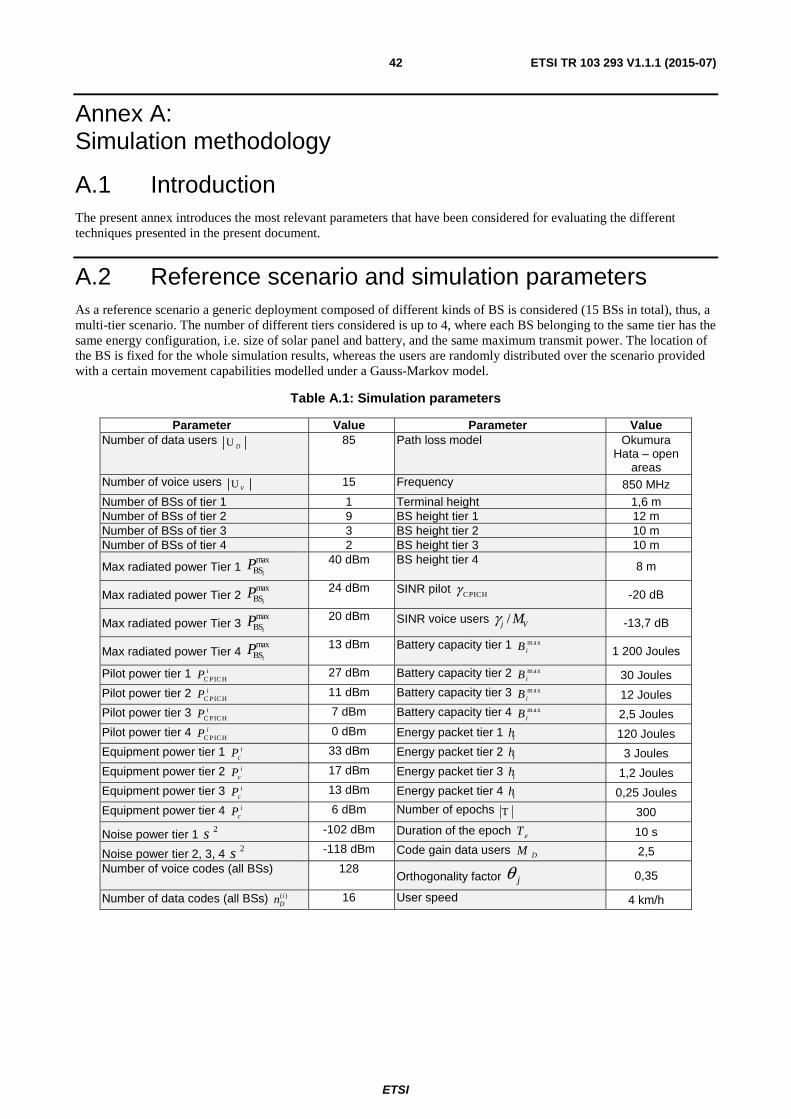
ETSI

ETSI TR 103 293 V1.1.1 (2015-07) 42

Annex A: Simulation methodology

A.1 Introduction The present annex introduces the most relevant parameters that have been considered for evaluating the different techniques presented in the present document.

A.2 Reference scenario and simulation parameters As a reference scenario a generic deployment composed of different kinds of BS is considered (15 BSs in total), thus, a multi-tier scenario. The number of different tiers considered is up to 4, where each BS belonging to the same tier has the same energy configuration, i.e. size of solar panel and battery, and the same maximum transmit power. The location of the BS is fixed for the whole simulation results, whereas the users are randomly distributed over the scenario provided with a certain movement capabilities modelled under a Gauss-Markov model.

Table A.1: Simulation parameters

Parameter Value Parameter Value Number of data users

DU 85 Path loss model Okumura Hata – open

areas Number of voice users

VU 15 Frequency 850 MHz Number of BSs of tier 1 1 Terminal height 1,6 m Number of BSs of tier 2 9 BS height tier 1 12 m Number of BSs of tier 3 3 BS height tier 2 10 m Number of BSs of tier 4 2 BS height tier 3 10 m

Max radiated power Tier 1 max

BSiP

40 dBm BS height tier 4 8 m


BSiP

24 dBm SINR pilot CPICHγ -20 dB


BSiP

20 dBm SINR voice users / Vj Mγ -13,7 dB


BSiP

13 dBm Battery capacity tier 1 m axiB 1 200 Joules

Pilot power tier 1 C PIC HiP 27 dBm Battery capacity tier 2 m ax

iB 30 Joules


iB 12 Joules


iB 2,5 Joules

Pilot power tier 4 C PIC HiP 0 dBm Energy packet tier 1 ih 120 Joules

Equipment power tier 1 icP 33 dBm Energy packet tier 2 ih 3 Joules

Equipment power tier 2 icP 17 dBm Energy packet tier 3 ih 1,2 Joules

Equipment power tier 3 icP 13 dBm Energy packet tier 4 ih 0,25 Joules

Equipment power tier 4 icP 6 dBm Number of epochs T 300

Noise power tier 1 2s -102 dBm Duration of the epoch eT 10 s

Noise power tier 2, 3, 4 2s -118 dBm Code gain data users DM 2,5 Number of voice codes (all BSs) 128

Orthogonality factor jθ 0,35

Number of data codes (all BSs) ( )iDn 16 User speed 4 km/h

ETSI

ETSI TR 103 293 V1.1.1 (2015-07) 43

The deployment layout is shown in figure A.1, where the colour code shows the number of available BSs at each point of the scenario. The number of detectable BSs depends on the power transmitted, and hence on the interference level. On its turn, the transmitted power may depend on the battery level and hence the coverage areas shown in figure A.1 change from epoch to epoch. In particular, figure A.1 shows the coverage regions when the batteries are full and the BSs are transmitting at maximum power. As it can be seen, the number of detectable BSs ranges from 1 BS up to 4 BSs

in given areas. All the points in figure A.1 fulfil the minimum SINR pilot requirements ( )CPICHg .

Figure A.1: Reference scenario and available BSs at a given epoch

A.3 Power consumption model and battery dynamics In this clause, the power consumption and the battery models are considered. The overall power consumption at any BS is modelled as the sum of the radiated power PRF (the power devoted to the pilot channels plus the power consumed by the traffic channels) and a fixed power consumed by the electronics of the BS, P0. The latter may include power consumption of the radio frequency (RF) chains, the baseband power consumption, and the cooling systems. The power consumption model considered in the simulations is the one provided by EC Project Earth depends on the number of radio transmitters NTRX, and the power spent when the radios are in sleep mode Psleep, as follows:

( )0 max

0

, 0

, 0

2 4,8 W 8 2,9 W

TRX p RF RF

in

TRX sleep RF

TRX p sleep

N P P P PP

N P P

N P P

⎧ + Δ < ≤⎪= ⎨=⎪⎩

= = Δ = = A.1

where the provided constants values are defined for HNB.

The overall energy consumption by the i -th BSs during the t -th epoch is:

( ) ( )( )i i ii e CPICH BS cE t T P P t P= + + A.2

where C P IC HiP is the power devoted to the pilot channels by the i -th BS, BS

iP stands for the power to be used for

traffic requests and icP models the fixed consumed power . It is assumed that the amount of power that can be used for

traffic services is limited in each BS. Such maximum traffic power depends on the particular tier and will be denoted as max

BSiP , so

maxBS BS( ) ,

i

iP t P i≤ ∀ .

ETSI

ETSI TR 103 293 V1.1.1 (2015-07) 44

Let Bi(t) be the energy stored at the battery of the i -th BS at the end of the epoch. Then at the beginning of the epoch t+1, the battery level is updated in general as

( ) ( ) ( ) ( )( )1 , , ,i i i iB t f B t E t H t t T+ = ∀ ∈ A.3

where Hi(t) is the energy harvested in Joules during the whole epoch t and the function depends upon the battery dynamics, such as storage efficiency and memory effects. A good approximation in practice is given by:

( ) ( ) ( ) ( ){ }{ }max1 max 0 m ,, in ,i i i i iB t B t E t H t B t T+ = − + ∀ ∈ A.4

where maxiB is the battery capacity, the inner minimization accounts for possible battery overflows, and the outer

maximization assures that the battery levels are non-negative. Note that Bi(t) follows a first-order Markov model that depends only on the immediate past state. Notice also that the whole harvesting collected during epoch t is included in the battery just at the end of the epoch for simplicity.

A.4 Energy harvesting model A discretized model for the energy arrivals is assumed where Hi(t), the energy harvested during the whole epoch t, is modelled as a stationary and ergodic Bernoulli process (which is a particular case of a Markov chain). As a result, only two values of harvested energy are possible during one epoch, i.e. , where hi is the amount of Joules

contained in an energy packet. For simplicity, it is considered that all BSs belonging to the same tier are provided with the same kind of energy harvesting source, hence, hi is the same for all BSs belonging to the same tier. The probability of receiving an energy-harvesting packet during one epoch is denoted by pi. Note that increasing pi would be equivalent

to increasing the harvesting intensity. In the case of solar harvesting, as the harvesting source is the same

for all BSs if they are located relatively close to each other.

A.5 Daily traffic profile In this clause, a brief summary of the daily traffic models used throughout this report is shown. For a more complete description of the models and assumptions, see TUCAN3G D41 [i.8].

A different daily traffic model has been assumed for the voice traffic and for the data traffic. Figure A.2 and figure A.3 depict the corresponding evolution of the normalized daily traffic assumed for the rural areas under consideration. In order to obtain the specific traffic rate in calls per second or packet served rate for the different locations described in TUCAN3G-D41 [i.8] (Santa Clotilde, Negro Urco, San Gabriel, San Juan and Tuta Pisco).

Figure A.2: Normalized daily voice traffic

( ) { }0, ,i ihH t i∈ ∀

ETSI

ETSI TR 103 293 V1.1.1 (2015-07) 45

Figure A.3: Normalized daily data traffic

Data concerning the number of inhabitants, the number of active users, and so on is needed to obtain the final traffic curves. Before explaining the procedure to obtain the aggregated arrival packet rate, let us introduce table A.2 with information of each specific location.

Table A.2: Traffic information of the different locations

Location Number of inhabitants

Number of inhabitants +

people in itinerancy

Average number of

subscribers

Average number of data users

Aggregated voice traffic

Santa Clotilde 2 685 3 222 1 707,66 85,383 17,077 Er Negro Urco 263 316 167,27 8,3635 1,673 Er Tuta Pisco 287 344 182,53 9,1266 1,825 Er San Gabriel 790 948 502,44 25,122 5,024 Er San Juan 98 118 62,33 3,1164 0,623 Er

In order to work out the aggregated arrival packet rate, the following assumptions are adopted:

• Penetration rate: 53 %

• Itinerancy: 20 %

• Active users during busy hour: 30 %

• Data users: 5 %

• Per-user arrival packet rate:

• Voice call generation rate:

Given the previous data, the aggregated arrival packet rate for the voice users is computed as:

A.5

where p is the number of inhabitants in each specific location and v(t) is the curve shown in figure A.2. The aggregated arrival packet rate for the data users is similarly computed as

A.6

where d(t) is the curve shown in figure A.3.

ETSI

ETSI TR 103 293 V1.1.1 (2015-07) 46

For an effective evaluation of the economical returns, the traffic forecast in the forthcoming years has to be considered. Such traffic evolution will be used for dimensioning purposes. The increments in the daily traffic, both for the voice traffic and the data traffic, for the forthcoming four years are + 180 %, + 5 %, + 2 %, and + 2 %, relative to the starting year.

ETSI

ETSI TR 103 293 V1.1.1 (2015-07) 47

History

Document history

V1.1.1 July 2015 Publication

tr 103 293 - v1.1.1 - broadband radio access networks ... · pdf filebroadband radio access...

Documents