Towards the consistent hydrological simulation using SWAT model.

Case Study: Vilcanota Andean basin in Peru

Carlos Antonio Fernández-palomino (cafpxl@gmail.com) 1,2; Fred F. Hattermann1; Waldo S Lavado-Casimiro 1;Fiorella Vega-Jácome 1;César L Aybar-Camacho 1; Oscar G Felipe-Obando 1;

1 2

What is the primary problem during the model calibration procedure?• Uncertainty in the determination of model parameters, owing to

the mismatch between model complexity and available data (Devak and Dhanya, 2017; Razmkhah et al., 2017).

To overcome this issue, recent studies have highlighted that the well-known sensitivity analysis (SA) of model parameters must be carried out prior to calibration (Devak and Dhanya, 2017; Shen et al., 2012; Song et al., 2015).

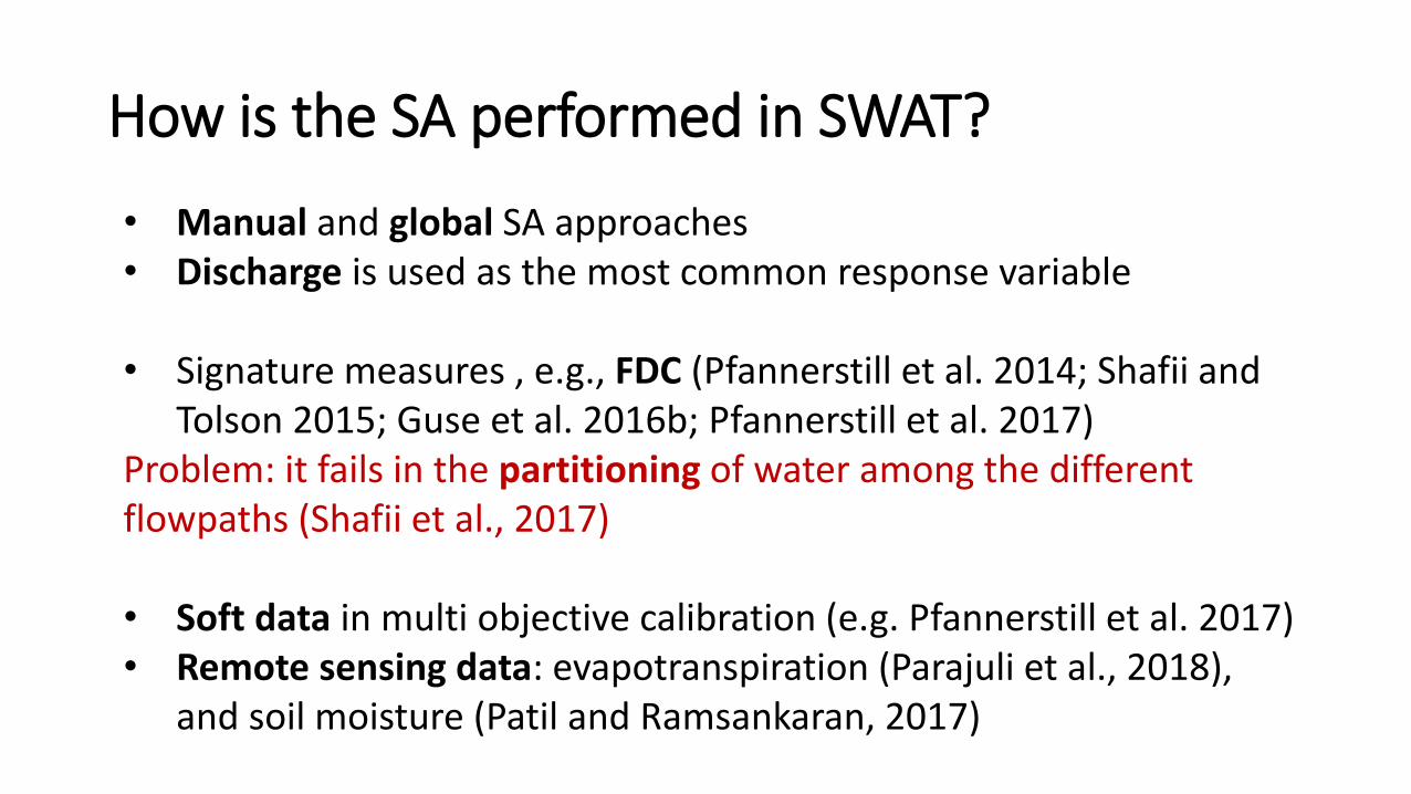
How is the SA performed in SWAT?

• Manual and global SA approaches• Discharge is used as the most common response variable

• Signature measures , e.g., FDC (Pfannerstill et al. 2014; Shafii and Tolson 2015; Guse et al. 2016b; Pfannerstill et al. 2017)

Problem: it fails in the partitioning of water among the different flowpaths (Shafii et al., 2017)

• Soft data in multi objective calibration (e.g. Pfannerstill et al. 2017)• Remote sensing data: evapotranspiration (Parajuli et al., 2018),

and soil moisture (Patil and Ramsankaran, 2017)

Problem in automatic SA and Calibration

• Inter-actions among SWAT parameters (Zhang et al. 2018)• Not considered by sampling design schemes (Devak and Dhanya,

2017; Razmkhah et al., 2017; Song et al., 2015)• Automatic methods can not control the equifinality or non-

uniqueness issue.

Consequently, using automatic methods unrealistic parameter values could result despite good performance statistics.

Objective

This study aims to improve the parameter identification in order to achieve hydrologically consistent parameter set.

RootZoneVadoseZoneShallowAquifer

Confining LayerDeep Aquifer

Fig. hydrological processes that are simulated by SWAT

Surface (Qsurf)runoff

Return flow (Qgws)from shallow aquifer

Recharge todeep aquifer

EvapotranspirationPrecipitation

Subbasin

Water

Sediments

Nutrients

HRU

soilcrop

slope

Soil and Water Assessment Tool (SWAT) - USDA

outputs

InputsWheatherSoilLand useDEM

Infiltration/ plant uptake/ Soil moisture redistribution

Revap. FromShallow Aquifer

Percolation toshallow aquifer

Wateryield(WYLD)

Defined by unique combination of:

Lost from the system(Neitsch et al., 2011)

Return flow (Qgwd)from deep aquifer

SWAT rev. 664 sourceBaseflow• Suggestion: the official SWAT literature needs to be updated regarding the deep

aquifer behavior.• Be careful with SWAT Check program in the baseflow index estimation

Proposed methodology: Multi-objective Process-Based sensitivity analysis.

Streamgauge

• hydrological processes Evapotranspiration, surface runoff and baseflow quantification

Where is analyzed the parameter influence on:• Model performance on discharge simulationNash-Sutcliffe – NSE, Percentage of bias - PBIAS

Confining Layer

Surface (Qsurf)runoff

Return flow (Qgws)from shallow aquifer

Return flow (Qgwd)from deep aquifer

Evapotranspiration

Baseflow (BF)

Wateryield(WYLD)

SWAT_BFI (BF/WYLD) equal to BFI estimated by the baseflow filter program (BFLOW)Desired values:

NSE=1, PBIAS=0%

Figure: Location of the study area and hydrometeorological stations network

Surface: 9613 km2

Altitudes ranging from2124 to 6309

Precipitation: 800 mm/year(>80 % ; October – March)

Daily discharges:30 m3/s (dry season) to 1100 m3/s (rainy season)

Average daily discharge :133 m3/s

Hydrological simulation for Vilcanota river basin

Data

Type of data Resolution Source Link

Hydrometeorological

dataDaily

SENAMHI and

EGEMSAhttp://www.senamhi.gob.pe/

DEM 90 m CGIAR-CSI http://srtm.csi.cgiar.org/

Land cover 300 m ESA CCI-LC http://maps.elie.ucl.ac.be/CCI/viewer/

Soil map 1:5 000 000 FAO-1995, 2003 http://www.waterbase.org/download_data.html

Table : Data type, resolution and data source

Time

Disc

harg

e [Q

, m3/

s]

2004-01-01 2006-01-01 2008-01-01 2010-01-01

NSE: 0.26PBIAS %: -17.1

0

500

1000

1500

2000 0102030

Prec

ipita

tion

[mm

/day

]

Q observed Q simulatedPrecipitationCN2: Curve numberSOL_BD: wet bulk densitySOL_AWC: available water capacityGWQMN: water depth threshold needed in shallow aquifer so that return flow occurs.RCHRG_DP: recharge fraction into the deep aquifer.

Initial simulation of the model

SWAT parameters sensitivity analysis

Relative change (Δ)

0100200300400500

a) Qsurf [mm]

0100200300400500

b) Qlat [mm]

0100200300400500

c) Qgw [mm]

0.00.20.40.60.81.0

-0.4 -0.2 0.0 0.2 0.4

d) SWAT_BFI

0.00.20.40.60.81.0

-0.4 -0.2 0.0 0.2 0.4

e) NSE

-40-200

2040

-0.4 -0.2 0.0 0.2 0.4

f) PBIAS [%]

BFI CN2

BFLOWBFI

0.78

Initial values

Good NSE but unrealistic representation on Surface runoff and BFI

SOL_BD

CN2 calibration is no necessary since ↑SOL_BD improves SWAT_BFI, NSE, PBIAS

SOL_AWC

SOL_AWC ↓ improves PBIAS

CN2: Curve numberSOL_BD: wet bulk densitySOL_AWC: available water capacity

“v”: replaced “r”: relative change

Order Parameter RangeAjusted

value1 SURLAG(v) [0.2, 0.5] 0.20

2 SOL_BD(r) [0.2, 0.5] 0.34

3 SOL_AWC(r) [-0.5, -0.2] -0.33

4 GWQMN(v) [600, 700] 681.30

5 RCHRG_DP(v) [0.3, 0.5] 0.36

GWQMN [mm]

0.20.40.60.81.0

0 1 2 3 4

g) NSE

-18-16-14-12-10

500

600

700

800

900

1000

h) PBIAS [%]

Table: Parameter values of the calibrated SWAT model

Initial value

SURLAG [unitless]

SWAT parameters sensitivity analysis

• ↓SURLAG improves NSE• ↓GWQMN improves PBIAS

observed versus simulated hydrograph

Disc

harg

e [Q

, m3/

s]

2004-01-01 2006-01-01 2008-01-01 2010-01-01 2012-01-01 2014-01-01

Calibration Validation

NSE: 0.73, PBIAS %: 0.8P-factor: 0.57, R-factor: 0.33

NSE: 0.79, PBIAS %: -2.2P-factor: 0.63, R-factor: 0.34

0

500

1000

1500

2000 0102030

Daily simulation

2004-01-01 2006-01-01 2008-01-01 2010-01-01 2012-01-01 2014-01-01

NSE: 0.95, PBIAS %: 0.8P-factor: 0.74, R-factor: 0.3

NSE: 0.95, PBIAS %: -2.4P-factor: 0.8, R-factor: 0.29

0200400600800

1000 0100200

Monthly simulation

Prec

ipita

tion

[mm

]

Q simulated (95PPU)Precipitation Q observed

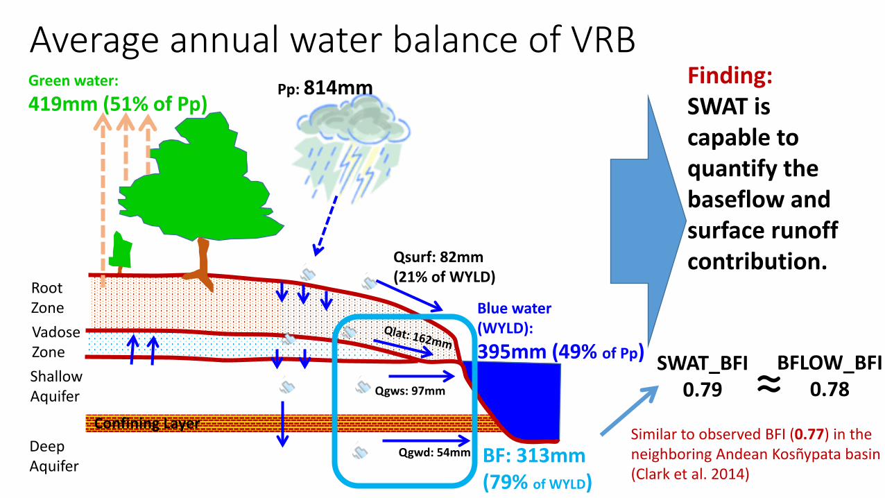
RootZoneVadoseZoneShallowAquifer

Confining LayerDeep Aquifer

Qsurf: 82mm(21% of WYLD)

Qgws: 97mm

Qgwd: 54mm

Green water: 419mm (51% of Pp)

Pp: 814mm

Average annual water balance of VRB

BF: 313mm(79% of WYLD)

Blue water(WYLD): 395mm (49% of Pp)

Finding: SWAT is capable to quantify the baseflow and surface runoff contribution.

SWAT_BFI0.79

BFLOW_BFI0.78≈

Similar to observed BFI (0.77) in the neighboring Andean Kosñypata basin(Clark et al. 2014)

Water potential (Qsurf + Qbf)

Water yield (WYLD)

mm

80%

20%

Conclusion

The results demonstrated that the set of sensitive parameters obtained with our approach provided consistency of SWAT results regarding the water balance components and discharges simulation.

Suggestions

Realistic hydrological simulation based on process-based calibration should be used for an appropriate assessment of:

• Basin hydrological processes,• Sediments quantification,• Land use change,• Climate change, • Usefulness of satellite-based precipitation in hydrological modeling

and other hydrological studies.