Ultramicroscopy 146 (2014) 130–143

Contents lists available at ScienceDirect

Ultramicroscopy

0304-39http://d

n CorrE-m

journal homepage: www.elsevier.com/locate/ultramic

Towards easy and reliable AFM tip shape determination using blindtip reconstruction

Erin E. Flater a,n, George E. Zacharakis-Jutz a, Braulio G. Dumba a,Isaac A. White a, Charles A. Clifford b

a Department of Physics, Luther College, 700 College Drive, Decorah, Iowa 52101, United Statesb Surface and Nano-Analysis, National Physical Laboratory, Hampton Road, Teddington, Middlesex TW11 0LW, United Kingdom

a r t i c l e i n f o

Article history:Received 13 August 2012Received in revised form18 May 2013Accepted 20 June 2013Available online 9 July 2013

Keywords:AFMSPMTip shapeTip characterizationBlind tip reconstruction

91/$ - see front matter & 2014 Elsevier B.V. Ax.doi.org/10.1016/j.ultramic.2013.06.022

esponding author. Tel.: +1 563 387 1632; fax:ail address: flater01@luther.edu (E.E. Flater).

a b s t r a c t

Quantitative determination of the geometry of an atomic force microscope (AFM) probe tip is critical forrobust measurements of the nanoscale properties of surfaces, including accurate measurement of samplefeatures and quantification of tribological characteristics. Blind tip reconstruction, which determines tipshape from an AFM image scan without knowledge of tip or sample shape, was established most notablyby Villarrubia [J. Res. Natl. Inst. Stand. Tech. 102 (1997)] and has been further developed since that time.Nevertheless, the implementation of blind tip reconstruction for the general user to produce reliable andconsistent estimates of tip shape has been hindered due to ambiguity about how to choose the key inputparameters, such as tip matrix size and threshold value, which strongly impact the results of the tipreconstruction. These key parameters are investigated here via Villarrubia's blind tip reconstructionalgorithms in which we have added the capability for users to systematically vary the key tipreconstruction parameters, evaluate the set of possible tip reconstructions, and determine the optimaltip reconstruction for a given sample. We demonstrate the capabilities of these algorithms throughanalysis of a set of simulated AFM images and provide practical guidelines for users of the blind tipreconstruction method. We present a reliable method to choose the threshold parameter correspondingto an optimal reconstructed tip shape for a given image. Specifically, we show that the trend in how thereconstructed tip shape varies with threshold number is so regular that the optimal, or Goldilocks,threshold value corresponds with the peak in the derivative of the RMS difference with respect to thezero threshold curve vs. threshold number.

& 2014 Elsevier B.V. All rights reserved.

1. Introduction

The atomic force microscope (AFM) is a versatile and powerfultool for the analysis of topographical and interfacial properties ofsurfaces with nanoscale resolution. Quantitative AFM is limited bythe geometry of the probe tip used to scan the surface, whichmeans that accurate knowledge of the AFM tip shape is critical foraccurate dimensional [1], nanomechanical [2], frictional force [3],chemical force [4], electrical force [5], and magnetic force mea-surements [6]. Typical scanning probe imaging modes allow a tipof finite geometry to move over a sample surface while maintain-ing a nominally constant tip-surface separation in order to rendera topological image of the surface. In the language of mathematicalmorphology, the topographical image produced is the dilation ofthe surface by the tip (more specifically the tip reflected throughits apex) [7]. Note that dilation is not the same as convolution,

ll rights reserved.

+1 563 387 1080.

since convolution is a linear mathematical process, and theprocess of dilation, by which an image is created by the physicalinteraction of tip and sample, is non-linear [8].

As is shown in Fig. 1, a tip that is sharper than the surfacefeatures will more accurately reproduce those features in an image(Fig. 1a) than a blunter tip (Fig. 1b). Images produced with a tipwhose geometrical features are of the same order as or larger thanthe surface features (Fig. 1b) will produce image features that canbe significantly broadened relative to the true surface geometry.Such measurements therefore cannot be relied upon for accuratelateral dimensional measurements of nanoscale surface features.While conventional AFM imaging exhibits some fundamentallimitations, including the inability of the tip to image undercutfeatures (as exemplified by a tip imaging a nearly spherical featurein Fig. 1), some techniques have been developed to minimize theselimitations [9,10]. Nevertheless, the measured height of imagedfeatures in conventional AFM will usually be accurate even thoughthe image widths may not be, provided that the AFM is indimensional calibration and the sample is sufficiently stiff towithstand imaging forces.

Fig. 1. Representations of AFM image profiles (bold line) produced for a surfacewith sharp and spherical features when imaging with (a) a sharp tip or (b) a blunttwo-peak tip.

E.E. Flater et al. / Ultramicroscopy 146 (2014) 130–143 131

Ever since the AFM was invented, users have sought sharp,robust, reproducible tips [11] of many different materials, includ-ing carbon nanotubes [12] or hard materials such as ultranano-crystaline diamond [13]. While quantification of tip size by themanufacturer is useful, even the most robust tip can experiencewear or mechanical shearing due to continuous or intermittentcontact with a surface during an AFM experiment [14,15], espe-cially if that experiment is performed in contact mode [16,17].The tip can also pick up contamination, such as nanoparticulatesor surface moieties, which can alter the chemistry and shape of thetip. Hence, for the most accurate tip shape determination, char-acterization is required before, during, and after an experiment.

There are two main methods used to characterize an AFMprobe tip shape [1] (a) ex situ direct imaging of the tip (typicallyusing electron microscopy) and (b) in situ indirect analysis thatleverages the fact that an AFM image is the mathematical dilationof the sample by the tip shape. Direct imaging is typicallyaccomplished using either a scanning electron microscope (SEM)or a transmission electron microscope (TEM). An SEM operated inbackscattered mode can produce images of an entire tip (includingapex, shank, and cantilever). Even some of the details of the tipapex on the order of tens of nanometers [18–20] can be deter-mined, and resolutions on the order of nanometer may beachieved with high resolution SEMs [21]. For nanometer andsubnanometer resolution of AFM tip features, a TEM is often used,although a TEM is typically limited to two-dimensional (2-D)shadow imaging unless multiaxis rotation stages within a TEMsample holder are available. Other disadvantages of electronmicroscopy include the potential for contamination by electronbeam-ionized residual gas [22–24], the time-intensive andimpractical necessity of removing the tip from the AFM, thedifficulty in determining the exact region of the tip that wouldcontact the surface, and the inability to image electrically insulat-ing AFM cantilevers and tips since material charging may preventstable high resolution imaging. In addition, immediate access tohigh quality electron microscopy instruments may be limited forsome users. Additional complications can occur when extractingthe exact tip shape from electron microscope images because ofintrinsic distortion and convolution effects in the images [25].

Indirect tip shape determination methods use AFM images todetermine the tip shape from samples whose surface geometriesmay be known or unknown [1]. Examples of tip characterizationsamples of assumed or known shape include, but are not limitedto: gold spheres and polystyrene spheres [26,27], cone-like struc-tures [28], holes and trenches [29], and carbon nanotubes [30].In these cases, deviations in the sample features from their ideal

size and shape, especially for nanoscale structures, will introduceerrors in the tip shape estimation. One must be particularly carefulthat reference samples do not change significantly with use (e.g.wear or contamination) [1], or that a method to re-characterizethe sample geometry exists.

If the surface geometry is unknown, an upper bound to the tipshape can be extracted from the image in a process known as blindtip reconstruction [7,31,32]. Any sample can be used, but a samplewith sharp features (e.g., TipCheck or NioProbe [MicroMasch, SanJose, CA]) provides blind tip reconstruction algorithms with morecomplete tip shape information, leading to more accurate tipreconstructions. Section 2 describes the mechanisms of the blindtip reconstruction method in detail. Blind tip reconstruction isadvantageous because it can be performed in situ. On the otherhand, commercial blind tip reconstruction algorithms can appearintractable to a user who seeks to quickly and easily determinetheir tip shape, specifically since the blind tip reconstructionprocess depends on a number of input parameters whose valuesare not obvious or intuitive and yet have a large impact on theresulting tip reconstruction. There are currently few guidelines onhow these parameter values should be chosen.

Here, we introduce a methodology that enables simple andreliable tip shape determination when using a blind tip recon-struction method for a given surface. Our main objective here is topresent clear protocols for the use of blind tip reconstructionalgorithms as a straightforward and reliable method to determinetip shape, which could form the basis of an international standardunder the auspices of ISO/TC 201/SC 9 in scanning probe micro-scopy. The algorithms used for this work are developed from thosefirst published by Villarrubia [7], and they are implemented inMATLAB (MathWorks, Natick, MA). The MATLAB code used for theresults in this paper will be available as open source code on theonline Nanoprobe Network Software Library. In this paper, thesealgorithms are applied to simulated AFM images (generated fromknown simulated surfaces and tips) from which the tip shape isthen reconstructed through the variation of relevant parameters.We thus demonstrate how a general user can reliably determinethe optimum reconstruction parameter values for their images.

2. Summary of the mathematics of blind reconstruction

There have been many contributions to the theory and practicalimplementation of blind reconstruction [7,8,31–39], and many ofthese and related methods have been reviewed here [1]. In thispaper we focus on the blind tip reconstruction algorithms devel-oped by Villarrubia [7]. Although improvements of these algo-rithms have been made since Villarrubia's initial publication of hiscode [1], the fundamental core of these methods has remained thesame. The mathematics of blind tip reconstruction depends on anumber of input parameters that must be optimized to generate abest estimate for the tip shape. For these reasons, a physicaldescription of the pertinent mathematical algorithms and relatedparameters is presented here for completeness and in order tomake the mathematics involved more intuitive.

Within blind tip reconstruction, the tip shape is determinedfrom an AFM image using an iterative process [7], which isrepresented schematically in Fig. 2 and will be described in theparagraphs that follow. While the original theoretical develop-ment of blind tip reconstruction uses the language and symbolismof mathematical morphology, the implementation of these ideaswithin Villarrubia's work (i.e., as implemented in the code) [7]can also be described in terms of the geometry of the tip andsample and their modification in the tip reconstruction process.We present a description of this “geometric representation” of theblind tip reconstruction to illustrate, from a slightly different

Fig. 2. A flowchart representing the key features of the blind tip reconstruction process. After initializing the tip shape estimate and reconstruction parameters, an imagecoordinate x′ is selected, and then a tip coordinate x is selected. For each permissible value of d (as dictated by Eq. (1)), the value of temp is calculated. The minimum absolutevalue for temp is determined and set equal to dil. If the variation of the image geometry near the tip contact point is sufficiently large compared with thresh (Eq. (3)), then thetip is modified at point x. This process is iterated for all possible x and x′ values until convergence occurs.

Fig. 3. Inverted tip and representative image profiles, indicating the application of the criterion of Eq (1). (a) A representative snapshot of one possible position where the tipcontacts the surface at tip coordinate d to produce the image point at x′. In this location, tip estimate modification does occur because the apex of the tip profile, located atx¼xc, is below the image profile (as dictated by Eq. (1)). (b) A representative snapshot of a position where it is not possible for the tip to contact the sample to produce theimage profile, as the apex (x¼xc) of the inverted tip profile lies above the image profile. This case represents the situation where the upright tip apex would penetrate thesample, which is physically impossible. Therefore this tip coordinate d cannot be used to modify the tip shape at x.

E.E. Flater et al. / Ultramicroscopy 146 (2014) 130–143132

perspective, the main features of these algorithms. In this paper,we use the same mathematical nomenclature as in Ref. [7].

The reconstruction procedure is shown schematically in Fig. 2and progresses as follows. First an initial estimate for an upperbound for the tip shape is chosen. We refer to the estimated tipshape hereafter as the tip estimate. Typically, a “square pillar” with

a flat top is used, where the surface of the tip consists of a matrixof zeros with dimensions that match the number of pixels chosenfor the size of the tip estimate. For example, a 20�20 pixel tipestimate is a 20�20 matrix of zeros. Since by definition the heightof the tip apex is fixed at zero height, the entire surface of the tiplies at the same height as the apex. As the tip estimate evolves

E.E. Flater et al. / Ultramicroscopy 146 (2014) 130–143 133

during the tip reconstruction process, tip heights may change, butall will remain less than or equal to zero. A 2-D profile of arepresentative matrix of zeros, i.e., a square pillar tip, is shown as arectangle in Figs. 3 and 4. Other initial tip estimates may be used,but this is the most general starting point.

Note that in Fig. 1b the tip geometry appears in the image as ifthe tip were reflected through its apex, i.e., as an inverted tip; thisis necessarily the case because the image is the dilation of thesurface by an inverted tip [7]. Therefore, for the purposes of tipreconstruction, the tip estimate is inverted (shown in Fig. 3 and inthe center of Fig. S1a in the Supplementary Material). After theinitial tip estimate is defined, the tip estimate is refined throughcomparison of the current tip estimate to the image geometry atevery point in the image.

Two-dimensional profiles of a representative image and aninitial tip estimate are shown in Fig. 3 and also in more detail inFig. S1. (An extension to three dimensions is straightforward.)Coordinates on the image are given as x′ and image heights arerepresented by the function I(x′). There are three coordinates ofinterest for the tip: a general tip coordinate x, the (fixed-height)center point of the tip xc, and the tip-image contact point d. Thispoint d on the tip corresponds with a chosen point x′ on the imageas a possible tip-sample contact point. P(x) is the height of the tipat any coordinate x, and is always less than or equal to zero, since P(x) represents the inverted tip.

After the tip estimate and reconstruction parameters areinitialized, the algorithm iterates through all possible values for x′(contact point) and x (tip refinement position). To determine ifrefinement can occur, the tip estimate is compared to the imagegeometry for all possible contact points (all possible d values).Modification of the tip estimate at x occurs only when

PðdÞ4 Iðx0Þ�Iðx0 þ xc�dÞ ð1ÞGeometrically speaking, the criterion described by Eq. (1)

allows for modification only if the tip apex coordinate xc is belowthe image profile for the particular d being considered. This isillustrated in Fig. 3, where two representations of potential d

Fig. 4. The process of modifying or refining the initial tip estimate. (a) The tip-surfacerecords the difference in height between the contact point and the height of the imagefound by varying d, or dil¼�min|temp|. (c) The tip height at x is then modified to a newexample x is located at the rightmost edge of the tip, and hence the modified portion o

contact points are shown. For the profile in Fig. 3a, refinementoccurs because the tip apex is below the image profile; whereasrefinement does not occur for the profile shown in Fig. 3b becausethe tip apex lies above the image profile. If Eq. (1) is satisfied, thetip apex never deviates from a zero height value, i.e., P(xc)¼0.

Next, the extent of tip estimate modification at tip coordinate xis determined. For every allowable tip refinement position, withcontact point at d on the tip and x′ on the surface (represented inFig. 4a), the value of

temp¼ Iðx′þ x�dÞ�Iðx′Þ þ PðdÞ ð2Þis calculated. The variable temp represents the difference betweenthe height of the image at x, i.e. I(x′+ x�d), and the height of theimage at x′, i.e., I(x′). The value of temp is computed for allallowable d values and the minimum absolute value of temp issaved as the variable dil (Fig. 4b). Once dil is found, the thresholdcriterion is applied to determine if tip estimate modificationactually occurs. The height of the tip at x is modified if dil is largeenough compared to the threshold value, thresh. This criterion fortip estimate modification at x is represented mathematically as

diloPðxÞ�thresh ð3ÞIf Eq. (3) is true, then the modification occurs (as is shown

in Fig. 4c, where thresh¼0 for simplicity) and the tip height atx is modified to

PðxÞ ¼ dilþ thresh ð4ÞIn the case of Fig. 4, initially thresh¼0 and P(x)¼0; therefore

since it is always true that dilo0, then Eq. (1) is true. Eq. (4) givesthe extent of the modification at x, which in this case is P(x)¼dil.If thresh was non-zero and dil is not large enough compared withthresh (i.e., Eq. (3) is false), then the point P(x) would haveremained unmodified.

The process described above is applied at every tip coordinate xfor the single image position x′. If the threshold value thresh is notzero, the modification will be less pronounced. For example, letthe value of thresh be 1 nm. Then P(x) will be modified as long as

image contact point x¼d is varied among all permissible points. The variable tempabove tip location x. (b) dil is determined as the minimum absolute value of tempheight so that it is lower than the previous height by the magnitude of dil. In thisf the tip is one pixel wide.

E.E. Flater et al. / Ultramicroscopy 146 (2014) 130–143134

dilo�1 nm. This criterion makes it less likely that P(x) will bemodified because the variation of the image profile over thedistance of x�d will need to be larger than 1 nm to produce alarge enough dil for the criterion dil¼max(I(x′+ x�d)� I(x′) ). Thenwhen the modification does occur (Eq. (1) is satisfied), the newvalue of P(x), which is equal to dil+thresh, will not be as large(in absolute value), since dilo0 and thresh40 (1 nm in thisexample case, so P(x) is 1 nm smaller in absolute value). Theprocess is repeated at every image location x′ within the image,and then the process iterates through the image again until the tipestimate P(x) converges.

As demonstrated in the above discussion, the input parameterthresh (the threshold value) is critical for the resulting tip recon-struction. If an image has no noise, then that image and theresulting tip reconstruction only contain information related to thetip and sample geometries. However, if the image contains noise,that noise could be mistaken in the tip reconstruction algorithmsas pertaining to the tip geometry. The threshold parameteraccounts for noise through the algorithms discussed above anddiscussed in reference [7].

The tip reconstruction user controls the threshold parameter,as well as the size of the initial tip shape estimate, namely itswidth (the size of the tip matrix). From a practical standpoint,some clear guidelines are necessary for selecting appropriatevalues of thresh and tip matrix size in order to produce anoptimum tip reconstruction. Some useful suggestions for choosingthese values have been given [7,20,35,37], but we wish to providea more concrete methodology for determining these parameters.Regarding tip matrix size, there is a fairly large permissible rangefor this parameter over which the tip reconstruction will beessentially independent [7]. Specific suggestions on how to choosethe tip matrix size are described in detail in Section 4.2.

The second major implication from the Villarrubia work is thatthere is a reproducible trend in the shape of the tip reconstructionas a function of threshold value. If the threshold value is too low inmagnitude, the tip reconstruction is dominated by high frequencynoise from the image. If, on the other hand, the threshold value istoo high, no features on the image are sharp enough to allow for a

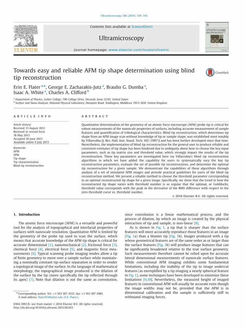
Fig. 5. The process of creating simulated images for evaluating the MATLAB-basedmathematically dilated by the simulated tip shape (top right) to produce the S imageGoldilocks tip reconstruction is identified (bottom).

modification of the initial “square pillar” tip geometry. Conse-quently, the reconstructed tip becomes unrealistically blunt. Theoptimum thresh value falls between these two extremes and isreferred to here as the “Goldilocks” threshold (neither too big nortoo small!).

3. Generation of simulated samples, tip, and images

3.1. Initial development of simulated sample surfaces, tip, andimages

To test the capabilities of these blind tip reconstruction algo-rithms and determine criteria for selecting tip reconstructionparameters, a set of simulated images were produced by mathe-matically dilating a simulated sample with a simulated tip. Thisprocess assumed non-deformable contacts. The simulated tip is≈38 nm wide at the base with a maximum height of 254 nm. Thistip also features two protrusions at right angles to each other, withtheir respective apexes positioned at 19 nm and 29 nm below theprimary tip apex (Fig. 5). This simulated tip has no reflectional orrotational symmetry to provide the most general tip shape. Blindtip reconstruction using simulated images, where the tip shape isknown, helps us determine optimal tip reconstruction parameterswhen knowledge of the tip shape is not available.

A number of distinct simulated surfaces were used; a representa-tive set of these simulated surfaces and their corresponding imagesare shown in Fig. 6. These surfaces were designed to be analogous inshape to typical AFM samples which could be used to characterizethe AFM tip shape, including: spikes (S); ridges (R), such as thoseformed by carbon nanotubes; and pitted, anodized alumina (P). Thesurfaces are not optimized to give tip reconstructions that mostaccurately reproduce the actual tip shape, but are simply meant torepresent relevant tip reconstruction surface geometries. All imagesconsist of 512�512 pixels, where each pixel is 1 nm in length alongthe x- and y-directions. In the z-direction, the maximum peak-to-valley height for all images was ≈290 nm.

blind tip reconstruction algorithms. The features of the S surface (top left) are(top center). From this image, various tip reconstructions are produced and the

E.E. Flater et al. / Ultramicroscopy 146 (2014) 130–143 135

The process of dilating the simulated sample and the simulatedtip is represented schematically in Fig. 5. From these simulatedimages, tip reconstructions were produced by varying the thresholdparameter over a sizeable range. For each image and set of tipreconstructions, the Goldilocks tip reconstruction was first identifiedby comparing the resulting tip reconstructions with the originalsimulated tip. The procedure for determining the Goldilocks tipreconstruction in cases where the tip shape is not known isexplained in Section 5.

3.2. Addition of noise to the simulated images

Tip reconstructions were generated from simulated imageswith added noise so as to use the tip reconstruction algorithms

Fig. 6. Representative simulated surfaces and resulting images used for evaluation of MAin this figure and all following figures have units of nanometers. (a) Spikes (S): Flat-top(analogous in shape to NioProbe from Aurora Nanodevices or TGT1 from NT-MDT). (b) Rfrom Aurora Nanodevices). (c) Pits (P): A series of paraboloidal pits (similar to anodized

to their full extent. Varying amounts of noise were incorporatedinto the simulated images, examples of which are shown in Fig. S2in the Supplementary material. A 512�512 pixel white noiseimage was generated with a root mean square (RMS) value of1 nm, and this noise image was scaled by a factor proportional toeach simulated image's z-range and then added to that image.For example, to create an image with a signal-to-noise (S/N) ratioof 160 where that image has a z-range of 200 nm, an imagecontaining only white noise with an RMS height value of (200/160)nm was added to the original image. In this paper, each image isreferred to by its identifying letter (corresponding to the samplesand images shown in Fig. 6) and the signal to noise ratio of theadded noise. For example, an image produced using the R samplewith an S/N ratio of 160 is referred to as R-160. For the analysis

TLAB-based blind tip reconstruction. The numbers indicated on the vertical scale barspikes with an in-plane apex radius of 3.5 nm and side walls of slope 95 nm/nmidges (R): Ridges with a roughly parabolic profile (analogous in shape to TipCheckalumina).

E.E. Flater et al. / Ultramicroscopy 146 (2014) 130–143136

that follows, tip reconstructions were performed on both noisyand noiseless images.

4. Details of the MATLAB-based blind tip reconstructionalgorithms

The blind tip reconstruction algorithms discussed in this paperwere coded in MATLAB and its algorithmic structure is diagramedin Fig. 7. The core of these algorithms is the original codepublished by Villarrubia [7]. This code, written in the C program-ming language, is directly accessed by the MATLAB algorithms.The original implementation in MATLAB was accomplished byTodd and Eppell [35] and allowed the user to produce one tipreconstruction at a time based on one set of tip reconstruction

Fig. 7. The procedural steps of the MATLAB-based blind tip reconstruction from the usermultiple tip reconstructions for multiple threshold values (bottom loop). These steps ar

parameters. We augmented these algorithms to produce a set oftip reconstructions for a range of threshold values, and to enablereal-time or off-line visualization analysis and facilitate the pro-cess of determining the Goldilocks tip reconstruction. The generalprocess of the algorithms’ implementation by users is as follows.

4.1. Import image into MATLAB

First the user imports an AFM image into MATLAB. The imagesimported into MATLAB for analysis can either be NanoScope datafiles (Bruker AFM, Santa Barbara, CA) or a text file. Multiple imagescan be loaded at the same time for rapid, serial image analysis. It isbest if the user apply a low pass or median filter on the imagebefore importing the image into MATLAB.

's perspective. The primary functionality added in this work is the ability to generatee described in detail in the sections indicated on the diagram.

E.E. Flater et al. / Ultramicroscopy 146 (2014) 130–143 137

4.2. Choose matrix size for reconstructed tip

The user then selects the matrix size for the reconstructed tip. Asdiscussed in Section 2, the fidelity of the Goldilocks tip reconstructionto the known tip estimate is invariant to the tip matrix size within acertain range [7]. When optimizing for both accuracy and timeefficiency, the user must choose a tip matrix size encompasses asufficiently wide range of image features, but one that is not so large asto become overly time intensive. The general guideline is to choose atip matrix size that has approximately the same lateral dimensions asthe largest recognizable tip artefact in the image. For example, inFig. 8 one can see in image S-80 the repeated feature resembling the

Fig. 8. Examples of how to choose the tip matrix size using (a) image type S, (b) image tyone can determine the appropriate choice of approximate tip matrix size to input into thtip reconstruction is insensitive to the tip matrix size within a reasonable range [7].

tip. The user chooses a tip matrix size equal to the dimension of oneof these features; this corresponds to a square region of about40�40 nm for the examples in Fig. 8. This choice of the tip matrixsize sets the initial tip estimate. For the P sample, the tip matrix sizeis approximately the width of the ridges between holes, as seen inFig. 8c.

4.3. Choose the threshold values

The user then chooses the threshold values to be used toproduce tip reconstructions. Each threshold value will correspondto one tip reconstruction. Since the threshold values are typically

pe R, and (c) image type P. By identifying the size of a representative image feature,e blind tip reconstruction algorithm. This size need not be exact, since the resulting

E.E. Flater et al. / Ultramicroscopy 146 (2014) 130–143138

proportional to the image z-range, the user's choice is scaledrelative to the image z-range. It is suggested that a first roughset of threshold numbers should be integer multiples of 5% of theimage z-range. Each threshold value is then tracked with adesignated threshold number to represent each threshold value.For example, if five threshold numbers were desired and theintervals were multiples of 5% of the image z-range, the thresholdvalues would be 0%, 5%, 10%, 15%, and 20% of the image z-range,and would be designated with threshold numbers of 0, 1, 2, 3, and4, respectively. Image S-80 has a z-range of 214.7 nm; hence, thesethreshold numbers would correspond to threshold values of 0 nm,10.7 nm, 21.5 nm, 32.2 nm, and 42.9 nm, respectively.

For maximum time efficiency of the tip reconstruction algo-rithms, threshold numbers are applied in reverse numerical order,starting with the largest threshold number. The first refinementbegins with the initial zeros matrix (square pillar) and applies thelargest threshold value. The tip shape estimate corresponding tothe largest threshold value is then used as the initial tip shapeestimate for the next highest threshold number reconstruction.This process is repeated until all threshold numbers have beenapplied and their tip reconstructions completed.

4.4. Choose additional thresholds if necessary

After the tip reconstructions are complete, the program dis-plays profiles of the tip reconstructions, and the user may analyzeindividual, three-dimensional tip reconstructions of interest. Thisfirst pass is made intentionally coarse to quickly assess the rangeof approximate values for the Goldilocks threshold parameter.The user is then given the option to produce additional tip recon-structions with a finer step (perhaps 0.1 threshold number steps,or steps of 0.5% of the image z-range, for the example given above)to isolate a particular set of tip reconstructions to refine further.We show in Section 5 that the blind tip reconstructions are similarwithin a range of threshold values, so the exact size of thethreshold step is not critical.

Fig. 9. Representative example of the result of a blind tip reconstruction, here from thethreshold values ranging from 0 nm to 107 nm. (b) Selected blind tip reconstruction profiles

5. Determining the Goldilocks threshold value and tipreconstruction

Determining the optimum value for the threshold parameterfor a given sample is the most important part of the blind tipreconstruction process whereby the most accurate tip reconstruc-tions are obtained for that sample. By applying a priori knowledgeof the tip shape used to produce our simulated images, we havedeveloped a method to guide the user in determining the Goldi-locks threshold value when a priori knowledge of the tip shape isnot available. We first discuss this methodology in the rare casewhere the actual tip shape is known (Section 5.1), and then discussthe more common case when the actual tip shape is not known(Section 5.2). We have applied these procedures to all the surfacesin Fig. 6, with images produced using a range of noise values (fromno noise to an S/N ratio of 20). We have also analyzed several othersets of simulated images, as well as real AFM images. The trendsdiscussed below are similar to the trends seen for all the imagesanalyzed.

5.1. Determining the Goldilocks tip reconstruction when the actualtip shape is known

Since the simulated images were used in this study, theresulting tip reconstructions were compared to the known actualtip shape and also the tip reconstruction generated from a noise-less version of each images set. We use the actual tip shape forcomparison since the main goal of a tip reconstruction user is toobtain the tip reconstruction that most accurately represents theactual tip shape. Since the simulated samples have finite geometry,even the most ideal tip reconstructions (those generated fromimages without noise) are not expected to exactly match theactual tip shape. For this reason, we present a comparison to theideal noiseless image tip reconstruction, as others have previouslydone [7,39].

Fig. 9a shows an example set of x- and y-direction profiles ofreconstructed tips produced from one of the images, in this caseP-80. Each tip profile along a given axis was constructed using a

P-80 profiles. (a) Twenty separate blind tip reconstruction profiles are shown, withwith threshold numbers close to the Goldilocks threshold number are shown for clarity.

E.E. Flater et al. / Ultramicroscopy 146 (2014) 130–143 139

different threshold value. Note that, as expected, for very largethreshold numbers, the tip shape estimate is identical to theoriginal square pillar, and for small threshold numbers, the tipreconstructions are dominated by image noise and therefore tendto be unrealistically sharp. For clarity, some of the profiles havebeen removed in Fig. 9b to show only the profiles that most closelymatch the known tip profile (which is shown in black in Fig. 9).By visual inspection, the largest tip with reasonable geometry thatmatches the known tip profile can be chosen as the best tip shapeestimate. For this particular set of tip reconstructions generatedfrom P-80, the best visual match occurs at threshold number 1.4(corresponding to a threshold value of 15.03 nm).

Although visual matching is sufficient when the actual tip shape isknown, a more quantitative and systematic method to determine theGoldilocks tip reconstruction is necessary, since in most cases theactual tip shape is not known. A comparison of the profiles using theRMS difference between the known and reconstructed profiles is usedto accomplish this task, which was previously used in [7]. Variousother quantitative measures exist and could be used, such as the tipprofile area [20], tip shape volume [10,39], or a tip radius approxima-tion [38]. Each technique comes with its own advantages anddisadvantages. For the case of tip profile area or tip shape volume,one must be careful when comparing areas or volumes, since thesame cross-section area or volume could result from drasticallydifferent profile shapes. For example, a jagged double peaked tipshape could have the volume as a smooth parabolic shape. Thereforethe area or volume does not constitute a unique measure of therelative accuracy of profiles or 3D tip shapes. The use of the radius ofcurvature to quantify the accuracy of a tip shape is not general enoughfor our purposes, because a parabolic fit that clearly identifies a tipradius may not always be possible or appropriate, as the tip may notresemble a parabolic shape. The RMS difference, on the other hand,gives a quantitative measure of comparison, which indicates howmuch a particular profile deviates from a reference profile, withoutmaking any assumptions about the tip shape. The RMS differencecomparison can be made evenwhen the tip reconstruction shape varydrastically or when no well-defined tip radius can be determined. TheRMS difference, as will be shown in this section, is a reliable measure

Fig. 10. Plots of RMS difference between the actual tip shape and each tip reconstructionthe Goldilocks threshold for the case when the true tip shape is known. On these graphsthe upper horizontal axis gives the threshold value in nm, which is proportional to the ththreshold. (b) RMS difference relative to the known tip profile with restricted profiles.

of deviation of a reconstructed tip profile from another tip profile(such as the known tip profile). Based on the definition of the RMSdifference, it is expected the threshold value for the Goldilocks tipreconstruction corresponds to a minimum RMS difference betweeneither the known actual tip shape profiles and reconstructed tipprofiles or the noiseless tip reconstruction profiles and the noisy tipreconstruction profiles.

Fig. 10a shows the RMS difference between the reconstructedx- and y-profiles and the respective known tip profile as a function ofthreshold (threshold number on the bottom horizontal axis, thresholdvalue on the top horizontal axis) for the P-80 image as an example.A definitive minimum in the RMS difference data is not apparent forboth x- and y-profiles even though the best visual match for this set oftip reconstructions occurs at threshold number 1.4. The lack of a well-defined minimum in the RMS difference curve of Fig. 10a occursbecause the reconstructed tip geometry does not closely match theknown tip geometry far from the tip apex. This deviation arises fromthe fact that an AFM-type image will only include a relatively smallpercentage of image points that contain information about the lowerpoints along the tip shaft, as has also been seen in other work [20].Deviation in the reconstruction between the two peaks of the actualtip is also expected for the same reason [20]. Therefore, estimated tipshape information far from the tip apex can be misleading, especiallyin context of the RMS difference curve of Fig. 10a. This motivates arestriction on the range of profile comparison to points near the tipapex. This restricted range lies between the vertical dashed lines inFig. 9. Thus, the restricted range coincides with the point at which theactual tip profile and the reconstructed tip profiles cross over oneanother. When this restriction is applied, the resulting RMS differencecurve (Fig. 10b) shows a distinct minimum occurring at the thresholdvalue corresponding to the Goldilocks tip reconstruction. A minimumalso occurs at the same Goldilocks threshold value when plotting theRMS difference relative to the noiseless image tip reconstruction vs.threshold. (See Supplementary material for more detail.)

However, in reality the actual tip shape and the noiseless imageare unavailable to the user, so these examples are only for proof ofconcept. Therefore a methodology is needed for cases whereneither the actual tip shape nor the noiseless image is available.

as a function of threshold value for image P-80. These plots are used to determineand the ones that follow, the lower horizontal axis gives the threshold number, andreshold number. (a) RMS difference relative to the known tip profile as a function of

E.E. Flater et al. / Ultramicroscopy 146 (2014) 130–143140

5.2. Determining the Goldilocks tip reconstruction when the tipshape is unknown

Since the reconstructed tip profiles change as a function ofthreshold value in a systematic way, the trend in the RMSdifference relative to a reference profile as a function of thresholdnumber can be used to determine of the Goldilocks tip reconstruc-tion when the actual tip shape is unknown. Any of the various tipreconstruction profiles could be used as a reference, but the profilecorresponding to a threshold value of zero is used. In other words,the RMS difference curve in Fig. 11a is tracking the deviation of thetip reconstruction profile shape relative to the tip reconstructionprofile produced when all of the image information is used(including image noise). Specifically, the RMS difference between

Fig. 11. Plots of RMS difference and its derivative between the zero threshold profile an(b) and P-20 for (c) & (d) as examples. These plots are used to determine the Goldilocks tto the zero threshold profile as a function of threshold for P-80. (b) Derivative of RMS diffcorresponds to the global maximum of the derivative for P-80. (c) RMS difference relativegradient than that of (a). (d) Derivative of the RMS (derivative of plot in (c)) as a functiondifference plot, the derivative plot (d) clearly shows a peak that corresponds to the Gol

a given profile and the zero threshold profile is calculated for eachthreshold number.

The methodology to find the Goldilocks threshold value isdescribed here using the representative examples in Fig. 11, andthis methodology was found to work for all the images analyzed.Starting at zero threshold number, the RMS difference relative tothat at zero threshold increases fairly slowly with threshold value(with a relatively modest slope from threshold number 0–1.2).As the threshold increases, the slope of the curve drasticallyincreases as the threshold nears the Goldilocks threshold (with ahigh slope from threshold number 1.2–1.4). The Goldilocks thresh-old occurs reliably after an abrupt (high slope) transition region,e.g., just after this high slope region (threshold number 1.4) inFig. 11a. As the threshold increases past the Goldilocks threshold,

d each tip reconstruction as a function of threshold value for image P-80 for (a) &hreshold without directly referring to the true tip shape. (a) RMS difference relativeerence (derivative of plot in (a)) as a function of threshold. The Goldilocks thresholdto the zero threshold profile as a function of threshold for P-20 showing a less stepof threshold for P-20. Even when the changes in slope are less dramatic in the RMSdilocks threshold for this image.

E.E. Flater et al. / Ultramicroscopy 146 (2014) 130–143 141

the slope of the RMS difference curve reduces again (with a lowslope again from threshold number 1.4 onward). In general, theGoldilocks threshold is consistently identified as the threshold forwhich the greatest change in slope occurs for the RMS differencerelative to the zero threshold. This trend in the RMS curve isconsistent regardless of surface type or level of noise (including,but not limited to, the simulated images shown in Fig. 6 & S2 andreal AFM images), and is also consistent with the trends seen byothers [20,35]. The physical explanation for this phenomenon isthat the abrupt transition between unphysically sharp tips to theGoldilocks tip shape occurs when the threshold is just largeenough to exclude image noise in order to produce the largesttip shape consistent with the true dilation of tip and sample [35].

An alternative way to find the Goldilocks threshold value isto calculate the derivative of the RMS difference relative to thex-direction and y-direction zero threshold profile. Such derivativeplots are shown in Figs. 11b, d, and 12b. The derivative is calculatedby taking the slope of the interval directly preceding a particulardata point on these graphs. For example, in Fig. 11b the derivativeindicated for threshold number 1 is the slope of the RMSdifference vs. threshold value curve over the interval of thresholdnumber 0 to threshold number 1. The peak in the derivative curveindicates the threshold number for which the tip reconstruction isoptimized. For example, in Fig. 11b, the derivative plot exhibits aglobal maximum at threshold number 1.4, indicating that 1.4 is theGoldilocks threshold number, in agreement with the Goldilocksvalue determined using the best visual match and using theminimum of the RMS difference with respect to the actual tipshape in Section 5.1. For some graphs of the RMS differencerelative to the zero threshold, the transition in slope is not asdramatic (for example, see Fig. 11c). In that case, the Goldilocksthreshold is not obvious from the plot of the RMS difference, butinstead can be easily identified from its derivative (Fig. 11d).

How can one be sure that one has found the Goldilocks tipreconstruction? It is possible that the transition to Goldilocksoccurred for a threshold number between 1.3 and 1.4? One way toaddress the ambiguity for the choice of Goldilocks threshold fromFig. 11a and b would be to investigate other possible thresholdnumbers between the threshold numbers 1.3 and 1.4. As shown in

Fig. 12. Plots of RMS difference and its derivative between the zero threshold profile anthreshold numbers are separated by increments of 0.01, instead of increments of 0.1 as shof threshold. (b) Derivative of RMS graph (derivative of plot in (a)) as a function of threshthere is a peak in the derivative plot for both x- and y-profiles.

Fig. 12, threshold number steps of 0.01 instead of 0.1 yield moreprecise values for the Goldilocks threshold. With this smallerinterval between thresholds, the transition region from lowthreshold number (1.2) to higher threshold number (1.4) containstwo distinct abrupt changes in RMS difference: one transitionaround threshold number 1.23, and another transition aroundthreshold number 1.35. These transition points are much moreclearly identified as spikes in the derivative (Fig. 12b). The reasonfor the double transition in this case is that the left hand side ofthe tip reconstruction profile makes the transition up to theGoldilocks shape first (around a threshold of 1.23) and then finallyat 1.35 the right side of the tip reconstruction profile thentransitions to the Goldilocks shape. For this reason, when a doubletransition occurs, the last abrupt transition in the RMS graphshould always correspond with the Goldilocks tip reconstruction.Hence, in this case the Goldilocks threshold corresponds with thethreshold number of 1.35. The minor peaks in Fig. 12b are causedby small variations in the tip reconstructions as the thresholdchanges. These variations are a natural consequence of the minutevariations in the tip reconstructions, which occur due to noise ofvarious frequencies in the image.

So which is the Goldilocks tip reconstruction? Fig. 9b showsprofiles from P-80 with Goldilocks threshold numbers of 1.3, 1.4,and 1.5. It can be seen that little quantitative difference existsbetween the tip reconstructions 1.4 and 1.5. The same is true forthe tip reconstruction profiles from threshold numbers of 1.35 and1.4 (not shown). In other words, any threshold value between 1.35and 1.5 would produce a reasonably accurate tip reconstruction.Calculating the difference between each of these profiles, we findthat the RMS difference from the actual tip profile deviates by atmost 6 nm between the profiles for threshold numbers 1.4 and 1.5(see Fig. 10). This insensitivity to threshold over a range of theGoldilocks threshold provides leeway as the user attempts to finda reasonable estimate for their tip shape. Hence, once there is anunambiguous sharp peak in the derivative plot that is consistentfor both the x- and y-profiles, no further refinement of thethreshold step is needed.

Using the methodologies described in this section, we demon-strate a reliable approach for determining the Goldilocks tip

d each tip reconstruction as a function of threshold for image P-80. In this case, theown in Fig. 11. (a) RMS difference relative to the zero threshold profile as a functionold. The Goldilocks threshold is identified as the highest threshold value for which

E.E. Flater et al. / Ultramicroscopy 146 (2014) 130–143142

reconstruction, even for noisy images and for cases where theGoldilocks threshold may be initially ambiguous.

6. Conclusions

The blind tip reconstruction method is a very powerful tool todetermine the shape of an AFM tip using a sample of unknownsurface geometry, which could simply be the primary sample to bestudied in the AFM experiment. Here, an overview of the blind tipreconstruction process was presented to make the process moreintuitive. We developed an augmented MATLAB-based implemen-tation of blind reconstruction that allows for easy variation of thekey input parameters: threshold value and tip matrix size. Thisalgorithm was used to investigate the role of these parameters, asimplemented using a set of simulated images. It was found that, ifthere are recognizably dilated features in the image, then the tipmatrix size is straightforward to determine. Specific guidelines fordetermining the optimum threshold number (the Goldilocksthreshold number) were developed. If the tip shape is known,then the Goldilocks threshold number identifies the tip recon-struction that occurs when the RMS difference with respect to theknown tip shape or the noiseless reconstruction is minimized.If, as is typically the case, the actual tip shape is not known, then itwas found that the Goldilocks tip reconstruction occurred at themaximum of the derivative of the RMS difference between profilesat a given threshold and those at zero threshold.

Acknowledgments

The authors thank Robert Carpick, Jingjing Liu, Vahid Vahdat,Graham Wabiszewski, and Kevin Turner at the University ofPennsylvania for fruitful discussions, comments, and analysesthrough the many phases of this work. We are also grateful toMick Phillips, formerly of the National Physical Laboratory, forinitial help generating the simulated images, and to AndrewYacoot of the National Physical Laboratory, Rachel Cannara of theNational Institute for Standards and Technology, and the refereesfor helpful comments. We acknowledge financial support from theAir Force Office of Scientific Research Grant FA9550-05-1-0204,the Luther College Dean's office, and the Luther College Emil C.Miller Fund for Physics. This work forms part of the UK Chemicaland Biological Metrology Programme of the UK National Measure-ment Systems Directorate of the UK Department for Business,Innovation and Skills.

Appendix A. Supporting information

Supplementary data associated with this article can be found inthe online version at http://dx.doi.org/10.1016/j.ultramic.2013.06.022.

References

[1] A. Yacoot, L. Koenders, Aspects of scanning force microscope probes and theireffects on dimensional measurement, J. Phys. D 41 (2008) 103001.

[2] C.A. Clifford, M.P. Seah, Quantification issues in the identification of nanoscaleregions of homopolymers using modulus measurement via AFM nanoinden-tation, Appl. Surf. Sci 252 (2005) 1915–1933.

[3] R.W. Carpick, N. Agraït, D.F. Ogletree, M. Salmeron, Measurement of interfacialshear (friction) with an ultrahigh vacuum atomic force microscope, J. Vac. Sci.Technol. B 14 (1996) 1289–1295.

[4] A. Noy, D.V. Vezenov, C.M. Lieber, Chemical force microscopy, Ann. Rev. Mater.Sci. 27 (1997) 381–421.

[5] T. Trenkler, T. Hantschel, R. Stephenson, P. De Wolf, W. Vandervorst,L. Hellemans, A. Malave, D. Buchel, E. Oesterschulze, W. Kulisch,

P. Niedermann, T. Sulzbach, O. Ohlsson, Evaluating probes for electrical atomicforce microscopy, J. Vac. Sci. Technol. B 18 (2000) 418–427.

[6] R.B. Proksch, T.E. Schaffer, B.M. Moskowitz, E.D. Dahlberg, D.A. Bazylinski,R.B. Frankel, Magnetic force microscopy of the submicron magnetic assemblyin a magnetotactic bacterium, Appl. Phys. Lett. 66 (1995) 2582–2584.

[7] J.S. Villarrubia, Algorithms for scanned probe microscope image simulation,surface reconstruction, and tip estimation, J. Res. Natl. Inst. Stand. Technol. 102(1997) 425–454.

[8] N. Bonnet, S. Dongmo, P. Vautrot, M. Troyon, A mathematical morphologyapproach to image formation and restoration in scanning tunneling andatomic force microscopies, Microsc. Microanal. Microstruct. 5 (1994) 477–487.

[9] N.G. Orji, R.G. Dixson, Higher order tip effects in traceable CD-AFM-basedlinewidth measurement, Meas. Sci. Technol. 18 (2007) 448–455.

[10] F. Tian, X. Qian, J.S. Villarrubia, Blind estimation of general tip shape in AFMimaging, Ultramicroscopy 109 (2008) 44–53.

[11] T.R. Albrecht, S. Akamine, T.E. Carver, C.F. Quate, Microfabrication of canti-lever styli for the atomic force microscope, J. Vac. Sci. Technol. A 8 (1990)3386–3396.

[12] Q. Ye, A.M. Cassell, H. Liu, K.-J. Chao, J. Han, M. Meyyappan, Large-scalefabrication of carbon nanotube probe tips for atomic force microscopy criticaldimension imaging applications, Nano Lett. 4 (2004) 1301–1308.

[13] K.-H. Kim, N. Moldovan, C. Ke, H.D. Espinosa, X. Xiao, J.A. Carlisle, O. Auciello,Novel ultrananocrystalline diamond probes for high-resolution low-wearnanolithographic techniques, Small 1 (2005) 866–874.

[14] T. Larsen, K. Moloni, F. Flack, M.A. Eriksson, M.G. Lagally, C.T. Black, Compar-ison of wear characteristics of etched-silicon and carbon nanotube atomic-force microscopy probes, Appl. Phys. Lett. 80 (2002) 1996–1998.

[15] P. Bakucz, A. Yacoot, T. Dziomba, L. Koenders, R. Krüger-Sehm, Neural networkapproximation of tip-abrasion effects in AFM imaging, Meas. Sci. Technol. 19(2008) 065101.

[16] J. Liu, J.K. Notbohm, R.W. Carpick, K.T. Turner, Method for characteriz-ing nanoscale wear of atomic force microscope tips, ACS Nano 4 (2010)3763–3772.

[17] J. Liu, D.S. Grierson, N. Moldovan, J.K. Notbohm, S. Li, P. Jaroenapibal, S.D. O'Connor, A.V. Sumant, N. Neelakantan, J.A. Carlisle, K.T. Turner, R.W. Carpick, Preventing nanoscale wear of atomic force microscopy tipsthrough the use of monolithic ultrananocrystalline diamond probes, Small 6(2010) 1140–1149.

[18] E. Buhr, N. Senftleben, T. Klein, D. Bergmann, D. Gnieser, C.G. Grase, H. Bosse,Characterization of nanoparticles by scanning electron microscopy in trans-mission mode, Meas. Sci. Technol. 20 (2009) 084025.

[19] J.A. DeRose, J.-P. Revel, Examination of atomic (scanning) force microscopyprobe tips with the transmission electron microscope, Microsc. Microanal. 3(1997) 203–213.

[20] L.S. Dongmo, J.S. Villarrubia, S.N. Jones, T.B. Renegar, M.T. Postek, J.F. Song,Experimental test of blind tip reconstruction for scanning probe microscopy,Ultramicroscopy 85 (2000) 141–153.

[21] D.C. Joy, J.B. Pawley, High-resolution scanning electron microscopy, Ultrami-croscopy 47 (1992) 80–100.

[22] U.D. Schwarz, O. Zworner, P. Koster, R. Wiesendanger, Preparation of probetips with well-defined spherical apexes for quantitative scanning forcespectroscopy, J. Vac. Sci. Technol. B 15 (1997) 1527–1530.

[23] M. Zharnikov, M. Grunze, Modification of thiol-derived self-assemblingmonolayers by electron and x-ray irradiation: scientific and lithographicaspects, J. Vac. Sci. Technol. B 20 (2002) 1793–1807.

[24] A. Vladar, M. Postek, Electron beam-induced sample contamination in theSEM, Microsc. Microanal. 11 (2005) 764–765.

[25] M.T. Postek, Critical issues in scanning electron microscope metrology, J. Res.Natl. Inst. Stand. Technol. 99 (1994) 641–671.

[26] K.A. Ramirez-Aguilar, K.L. Rowlen, Tip characterization from AFM images ofnanometric spherical particles, Langmuir 14 (1998) 2562–2566.

[27] P. Colombi, I. Alessandri, P. Bergese, S. Federici, L.E. Depero, Self-assembledpolystyrene nanospheres for the evaluation of atomic force microscopy tipcurvature radius, Meas. Sci. Technol. 20 (2009) 084015.

[28] M.P. Seah, S.J. Spencer, P.J. Cumpson, J.E. Johnstone, Sputter-induced cone andfilament formation on InP and AFM tip shape determination, Surf. Interf. Anal.29 (2000) 782–790.

[29] U. Hubner, W. Morgenroth, H.G. Meyer, T. Sulzbach, B. Brendel, W. Mirande,Downwards to metrology in nanoscale: determination of the AFM tip shapewith well-known sharp-edged calibration structures, Appl. Phys. A: Mater. Sci.Process. 76 (2003) 913–917.

[30] Y. Wang, X. Chen, Carbon nanotubes: a promising standard for quantitativeevaluation of AFM tip apex geometry, Ultramicroscopy 107 (2007) 293–298.

[31] P.M. Williams, K.M. Shakesheff, M.C. Davies, D.E. Jackson, C.J. Roberts, S.J.B. Tendler, Toward true surface recovery: studying distortions in scanningprobe microscopy image data, Langmuir 12 (1996) 3468–3471.

[32] P.M. Williams, K.M. Shakesheff, M.C. Davies, D.E. Jackson, C.J. Roberts, S.J.B. Tendler, Blind reconstruction of scanning probe image data, J. Vac. Sci.Technol. B 14 (1996) 1557–1562.

[33] J.S. Villarrubia, Morphological estimation of tip geometry for scanned probemicroscopy, Surf. Sci 321 (1994) 287–300.

[34] J.S. Villarrubia, Scanned probe microscope tip characterization without cali-brated tip characterizers, J. Vac. Sci. Technol. B 14 (1996) 1518–1521.

[35] B.A. Todd, S.J. Eppell, A method to improve the quantitative analysis of SFMimages at the nanoscale, Surf. Sci 491 (2001) 473–483.

E.E. Flater et al. / Ultramicroscopy 146 (2014) 130–143 143

[36] S. Dongmo, M. Troyon, P. Vautrot, E. Delain, N. Bonnet, Blind restorationmethod of scanning tunneling and atomic force microscopy images, J. Vac. Sci.Technol. B 14 (1996) 1552–1556.

[37] D. Tranchida, S. Piccarolo, R.A.C. Deblieck, Some experimental issues of AFMtip blind estimation: the effect of noise and resolution, Meas. Sci. Technol. 17(2006) 2630–2636.

[38] T. Machleidt, R. Kästner, K.-H. Franke, Reconstruction and Geometric Assess-ment of AFM Tips, in: Nanoscale Calibration Standards and Methods, Wiley-VCH Verlag GmbH & Co. KGaA297–310.

[39] G. Jozwiak, A. Henrykowski, A. Masalska, T. Gotszalk, Regularization mechan-ism in blind tip reconstruction procedure, Ultramicroscopy 118 (2012) 1–10.