Total Variation Regularization by Iteratively

Reweighted Least Squares on Hadamard

Spaces and the Sphere

P. Grohs and M. Sprecher

Research Report No. 2014-39December 2014

Seminar für Angewandte MathematikEidgenössische Technische Hochschule

CH-8092 ZürichSwitzerland

____________________________________________________________________________________________________

Funding SNF: 140635

Total Variation Regularization by Iteratively Reweighted

Least Squares on Hadamard Spaces and the Sphere ∗

Philipp Grohs Markus Sprecher

December 19, 2014

Abstract

We consider the problem of reconstructing an image from noisy and/or incomplete data, where the

image/data take values in a metric space X (e.g. R for grayscale, S2 for the chromaticity component

of RGB-images or SPD(3), the set of positive definite 3× 3-Matrices, for Diffusion Tensor Magnetic

Resonance Imaging (DT-MRI)). We use the common technique of minimizing a total variation (TV)

functional J. After having defined J for arbitrary metric spaces X we will propose an adaption of the Iter-

atively Reweighted Least Squares (IRLS) algorithm to minimize J. For the case of X being a Hadamard

space, such as SPD(n), we prove existence and uniqueness of a minimizer of a regularized functional Jε

where ε > 0 and show that these minimizers convergence to a minimizer of J when the regularization

parameter ε tends to zero. We show that IRLS can also be applied for X being a half-sphere. For the case

of X being a Riemannian manifold we propose to use Newton’s method on Manifolds to numerically

compute the minimizer of Jε . To demonstrate our algorithm we present some numerical experiments

where we denoise and/or inpaint sphere-valued and SPD-valued images.

Keywords: Iteratively reweighted least squares, total variation, regularization, manifold-valued data

1 Introduction

In many applications images are corrupted with some kind of noise. The common tasks of denoising is to

remove this noise while keeping the main features of the image unchanged. Furthermore the image might

not be known everywhere. The task of inpainting is to restore the image at the unknown regions.

1.1 Real-valued Images

In 1992, Rudin, Osher and Fatemi revolutionized the field of real-valued image denoising and restoration

with their celebrated paper [27]. Their approach is based on minimizing the total variation TV (u) =∫

Ω |∇u|of an image u : Ω → R subject to the constraints

∫

Ω u =∫

Ω a and∫

Ω(u− a)2 = σ2. Here a denotes the

noisy image and σ is a given constant. It was the first method which was able to remove noise while still

preserving edges. Chambolle and Lions [8] showed that the problem has a unique solution and is equivalent

to minimizing the TV-functional

J(u) =1

2‖u−a‖2

2 +λTV (u), (1)

∗The research of the authors was supported by the Swiss National Fund under grant SNF 140635.

1

where λ > 0 depends on σ . The functional J is especially useful to remove Gaussian noise. For noise types

with heavier tail such as Laplacian noise, the functional u 7→ ‖u− a‖1 +λTV (u) is more appropriate. A

discrete version of (1) can be found by using a finite difference discretization of ∇u. For 2D-images we

can find two different ways to discretize the total variation norm in the literature, the anisotropic version

TVaniso(u) = ∑i, j

|ui+1, j −ui, j|+ |ui, j+1 −ui, j| (2)

and the isotropic version

TViso(u) = ∑i, j

√

(ui+1, j −ui, j)2 +(ui, j+1 −ui, j)2. (3)

Several methods to find the minimizer of the discrete Versions of (1) have been proposed. For example

by using Fenchel duals [7], the alternating direction method of multipliers [33], and Split-Bregman meth-

ods [32].

1.2 Color Images

After Rudin et al. published their impressive denoising result on grayscale images, a logical next step was

to extend the TV method for color images. Various TV functionals ([4, 10, 17, 26] to mention but a few)

have been proposed with promising results. Initially, the two linear color models (the channel-by-channel

and the vectorial model) were examined before also nonlinear models for color image were studied ([10,

23, 28, 30]). One of them, the chromaticity-brightness model, turned out to be closer to human perception

than others. Chang and Kang [10] were able to present persuasive numerical results. Nevertheless, linear

models were in favor for quite a while, presumably due to their simplicity in comparison to the nonlinear

models.

1.3 Manifold-valued Images

Images taking values in a manifold appear naturally in various signal and image processing applications.

The most prominent example is DT-MRI. There are several proposals how to regularize DT-MRI images

[11, 12, 21]. Recently there has also been made progress in extending TV regularization to arbitrary Rie-

mannian manifolds. In [19] Lellmann, Strekalovskiy, Kotter and Cremers presented a first framework and

an algorithmic solution for TV regularization for arbitrary Riemannian manifolds. Their idea is to reformu-

late the variational problem as a multilabel optimization problem which then can be solved approximately

by convex relaxation techniques. They mentioned that “Many properties of minimizers of total variation-

regularized models in manifolds are still not fully understood”. In [31] Weinmann, Demaret and Storath

considered a generalization of the anisotropic (see Equation (2)) version of the discrete total variation to

Riemannian manifolds. They propose a proximal point algorithm to minimize their TV-functional and

prove convergence for data taking values in Hadamard spaces. Convergence results for spaces which are

not Hadamard is still an open problem.

2

1.4 Total Variation on Arbitrary Metric Spaces

We define the TV-functional for any metric space (X ,d). Let V be an index set of all the pixels of our

image (usually a two-dimensional grid). Our generalizations of the the total variation are

TVaniso(u) := ∑(i, j)∈E

d(ui,u j) and TViso(u) := ∑i∈V

√

∑j∈n(i)

d2(ui,u j), (4)

where E ⊂ V ×V is a set of edges and n(i) := j ∈ V |(i, j) ∈ E. Let a : Vk ⊂ V → X be the given noisy

image. Whenever possible we will drop the subscripts aniso and iso to indicate that the statement holds for

both cases. We can now define the generalized TV-functional J : XV → R by

J(u) :=1

2∑

i∈Vk

d2(ui,ai)+λTV (u). (5)

Throughout this document we will assume that (V,E) is connected and Vk is non-empty. However if (V,E)

is not connected and Vk contains at least one vertex of every connected component of V we can write J as

a sum of independent subfunctionals and the statements remain true.

1.5 Our Contribution

We present an adaption of the Iteratively Reweighted Least Squares (IRLS) algorithm to minimize the TV-

functional. IRLS has been proven to be very successful for recovering sparse signals [13] and was already

applied to scalar TV-minimization problems in [25]. We will prove convergence to a global minimizer

in the case of Hadamard spaces. Using new arguments and a result from differential topology, we show

that our algorithm is also applicable for the important case of X being a half-sphere. This result is of

independent interest and can also be seen as a first step towards a theory of convergence for spaces which

are not Hadamard. The fact that the IRLS algorithm can be interpreted as an alternating minimization

algorithm [13] will be very useful to obtain our results.

1.6 Outline

We have structured the article as follows. In Chapter 2 we define our adaption of the IRLS algorithm. It

generates a sequence for which the value of the TV-functional is decreasing. Under some conditions on

J we prove that this sequence converges to a minimizer of a regularized functional Jε . In Chapter 3 we

present the necessary theory of Hadamard spaces and prove that if X is a Hadamard space then J is convex

and satisfies the conditions from Chapter 2. We also prove that the regularized functional Jε has a unique

minimizer and these minimizers converge to a minimizer of J when ε tends to zero. Our algorithm for

TV-minimization for X being a Riemannian manifold is presented in Chapter 4. In Chapter 5 we show

that if X is a half sphere the functional of the optimization problem occurring in the IRLS algorithm has a

unique critical point. Finally in Chapter 6 we present details on the implementation and some numerical

experiments.

3

2 Iteratively Reweighted Least Squares

2.1 Definition of IRLS

The IRLS algorithm [13] alternates between reweighting and minimization steps. The generalization of the

algorithm is straightforward. Let ε > 0, the minimization and reweighting steps of the anisotropic case are

unew = argminu∈XV

∑i∈Vk

d2(ai,ui)+λ ∑(i, j)∈E

wi, jd2(ui,u j) and (6)

wnewi, j = W ε

aniso(u)i, j := (d2(ui,u j)+ ε2)−12 for all (i, j) ∈ E. (7)

Analogously the steps of the isotropic case are

unew = argminu∈XV

∑i∈Vk

d2(ai,ui)+λ ∑i∈V

wi ∑j∈n(i)

d2(ui,u j) and (8)

wnewi = W ε

iso(u)i :=

(

∑j∈n(i)

d2(ui,u j)+ ε2

)− 12

for all i ∈V. (9)

The parameter ε > 0 is necessary to avoid division by zero and is typically chosen very small. In the

literature [15] we also find the alternative reweighting defined by

wnewi, j = max

(ε,max(d(ui,u j),ε)

−1)

in the anisortropic case. However this reweighting seems to be more difficult to analyze and we will

therefore stick to the reweightings given in Equation (7) and (9). Note that for Euclidean spaces we have to

minimize a quadratic function in the minimization step. This can be done by solving a linear system which

is where the term least squares of IRLS comes from.

2.2 Analysis of IRLS

To analyze IRLS we use ideas of [9]. We define the regularized functionals Jεaniso and Jε

iso by

Jεaniso(u) :=

1

2∑

i∈Vk

d2(ui,ai)+λ ∑(i, j)∈E

√

d2(ui,u j)+ ε2, and (10)

Jεiso(u) :=

1

2∑

i∈Vk

d2(ui,ai)+λ ∑i∈V

√

∑j∈n(i)

d2(ui,u j)+ ε2. (11)

Remark 1. Although the functional Jε is smooth when X is a smooth Riemannian manifold the perfor-

mance of standard methods to find its minimizer (e.g. Newton) is poor. A possible explanation for this

observation is that Jε is highly nonlinear for ε small.

To view IRLS as an alternating minimization technique we define the two variable functionals

4

Jεaniso : RE

>0 ×XV → R and Jεiso : RV

>0 ×XV → R by

Jεaniso(w,u) :=

1

2∑

i∈Vk

d2(ui,ai)+1

2λ ∑

(i, j)∈E

wi, j(d2(ui,u j)+ ε2)+w−1

i, j , and (12)

Jεiso(w,u) :=

1

2∑

i∈Vk

d2(ui,ai)+1

2λ ∑

i∈V

wi

(

∑j∈n(i)

d2(ui,u j)+ ε2

)

+w−1i . (13)

We now show a connection between the critical points of Jε and Jε .

Lemma 2. The pair (w,u) is a critical point of Jε if and only if u is a critical point of Jε and w =W ε(u)

where W ε is defined in (7) for the anisotropic and in (9) for the isotropic case.

Proof. Note that

Jε(w,u) =1

2∑

i∈Vk

d2(ui,ai)+1

2λ ∑

i

wiWε(u)−2

i +w−1i (14)

Jε(u) =1

2∑

i∈Vk

d2(ui,ai)+λ ∑i

W ε(u)−1i . (15)

Hence we have

∂ Jε

∂wi(w,u) = 1

2λ (W ε(u)−2

i −w−2i ),

∂ Jε

∂u(w,u)

∣∣∣w=W ε (u)

= 12 ∑i∈Vk

∂d2(ui,ai)∂u

−λ ∑i Wε(u)−2

i∂W ε (u)i

∂u= dJε

du(u)

and∂ Jε

∂w(w,u) = 0 and

∂ Jε

∂u(w,u) = 0 ⇔ W ε(u) = w and

dJε

du(u).

The idea of alternating minimization is to fix one variable and to minimize the functional w.r.t. the

other variable and vice versa. Consider the sequences (w( j)) j∈N,(u( j)) j∈N recursively defined by

w( j+1) := argminw

Jε(w,u( j)), and (16)

u( j+1) := argminu∈XV

Jε(w( j+1),u) (17)

Note that Equations (16) and (17) are equivalent to Equation (6) and (7) respectively Equation (8) and (9).

Hence alternating minimization of Jε is equivalent to IRLS. An immediate consequence is that the value

of Jε is non-increasing.

Theorem 3. The sequence(

Jε(u( j)))

j∈Nis non-increasing.

Proof. Note that Jε(u) = Jε(W ε(u),u). Hence the statement follows by the interpretation of the IRLS-

algorithm as alternating minimization of Jε .

As explained in [24] alternating minimization can fail to converge to a minimizer. However under

the assumption that Jε has a unique critical point we can prove convergence. We will need the following

elementary topological Lemma.

5

Lemma 4. Let A be a compact space, B a topological space, f : A → B a continuous function, a ∈ A

such that f (x) = f (a) if and only if x = a and (x(i))i∈N ⊂ A a sequence with limi→∞ f (x(i)) = f (a). Then

limi→∞ x(i) = a.

Proof. Assume there exist an open neighborhood N(a) of a such that for infinitely many i ∈ N we have

x(i) /∈ N(a). As A\N(a) is compact there exist a subsequence(

x(ni))

i∈Nwhich converges to some a ∈

U\N(a). We now have

f (a) = limi→∞

f (x(ni)) = f (a).

which contradicts the assumption.

We are now able to prove the main result of this chapter.

Theorem 5. Assume that

i) Jε has a unique minimizer.

ii) u 7→ Jε(w,u) has a unique minimizer for all w ∈ RE>0

(resp.w ∈ R

V>0

).

Let u(0) ∈ XV , w(0) ∈ RE>0 (resp. w(0) ∈ R

V>0) and (w( j),u( j)) be defined by Equations (16) and (17). Then

the sequence u( j) converges to the unique minimizer of Jε .

Proof. Note that Jε(w( j),u( j)) is bounded from below and monotonically decreasing with j. Therefore

Jε(w( j),u( j)) converges to some value c ∈ R. Note that ‖w( j)‖ℓ∞ 6 ε−1 and the sequence (w( j),u( j)) is

bounded. Therefore it has a subsequence (w(n j),x(n j)) converging to some (w, u). Let

w′ := argminw∈RV

Jε(w, u), and u′ := argminu∈MV

Jε(w′,u).

We have

c = limj→∞

Jε(w(n j+1),u(n j+1)) = Jε(w′,u′)6 Jε(w′, u)6 Jε(w, u) = limj→∞

Jε(w(n j),u(n j)) = c.

As we have equality and the functions u 7→ Jε(w′,u) and w 7→ Jε(w, u) have unique minimizers we have

w′ = w and u′ = u. It follows that w = W (u) and (u, w) is a critical point of Jε . Therefore by Lemma 2 u

is the unique minimizer of Jε and (w, u) is the unique minimizer of Jε . Finally by Lemma 4 we get that

lim j→∞(w( j),u( j)) = (w, u).

3 TV on Hadamard Spaces

We start this chapter by the definition of Hadamard spaces, also known as spaces of non-positive curvature.

Definition 1. A complete metric space X is called a Hadamard space if for all x0,x1 ∈ X there is y ∈ X

such that for all z ∈ X we have

d2(z,y)61

2d2(z,x0)+

1

2d2(z,x1)−

1

4d2(x0,x1). (18)

A comprehensive introduction to the nowadays well-established theory of Hadamard spaces is [3]. The

space of positive definite matrices is a Hadamard space (see [5], Page 314). An important property of

Hadamard spacess is that for any two points there exist a unique geodesic connecting them.

6

Definition 2. A curve γ : [0,1]→ X, where X is a metric space is called a geodesic if

d(γ(t1),γ(t2)) = |t1 − t2|d(γ(0),γ(1)) for all t1, t2 ∈ [0,1].

To prove uniqueness of a minimizer of Jε we will need the notion of convexity.

Definition 3. A function f : X →R, where X is a metric space is called convex (resp. strictly convex) if for

every non-constant geodesic γ : [0,1]→ X the function f γ : [0,1]→ R is convex (resp. strictly convex).

Convexity will be important to get information on the set of minimizers.

Definition 4. A set C ⊂X is called geodesically convex if for any geodesic γ : [0,1]→X with γ(0),γ(1)∈C

we have γ(t) ∈C for all t ∈ [0,1].

Lemma 6. Let X be a Hadamard space. Then the set of minimizers of a convex function f : X → R is

geodesically convex.

The proof follows immediately from the theory of convex functions on R and the definition of geodesi-

cally convex sets. As in our TV-functional distances, respectively squared distances, occur, it is of interest

if d, respectively d2, is convex. For Hadamard spaces this is well-known and stated below.

Theorem 7 (Sturm [29]). Let X be a Hadamard space, d : X ×X → R its distance function and y ∈ X.

Then the function x 7→ d2(x,y) is strictly convex.

The prove follows by repeatedly using Equation (18). Note that if X is a Hadamard space then Xn with

the metric

d(x,y) :=

√n

∑i=1

d2(xi,yi) for all x = (xi)ni=1, y = (yi)

ni=1 ∈ Xn,

is also a Hadamard space.

Theorem 8 (Sturm [29], Ballmann (Prop. 5.4. in [3])). For a Hadamard space X the distance function

d : X2 → R is convex.

Corollary 9. If X is a Hadarmard space the functional Janiso : XV → R defined in (5) is convex.

Proof. This follows from Theorem 7 and Theorem 8.

To prove convexity of Jiso we need the following lemma.

Lemma 10. If f1, . . . , fn : [0,1]→ R>0 are convex functions then the function

√

f 21 + · · ·+ f 2

n is also con-

vex.

Proof. Note that by induction it suffices to prove the statement for n = 2. By convexity of f1 and f2 we

have

f1(t) 6 t f1(1)+(1− t) f1(0)

f2(t) 6 t f2(1)+(1− t) f2(0).

Squaring and adding the inequalities yields

( f 21 + f 2

2 )(t)6 t2( f 21 + f 2

2 )(1)+(1− t)2( f 21 + f 2

2 )(0)+2t(1− t)( f1(0) f1(1)+ f2(0) f2(1)).

7

By Cauchy-Schwarz we get

( f 21 + f 2

2 )(t) 6 t2( f 21 + f 2

2 )(1)+(1− t)2( f 21 + f 2

2 )(0)+2t(1− t)( f1(0) f1(1)+ f2(0) f2(1))

6 t2( f 21 + f 2

2 )(1)+(1− t)2( f 21 + f 2

2 )(0)+2t(1− t)√

f 21 + f 2

2 (1)√

f 21 + f 2

2 (0)

=

(

t

√

f 21 + f 2

2 (1)+(1− t)√

f 21 + f 2

2 (0)

)2

.

Taking the square root shows that the function

√

f 21 + f 2

2 is convex.

Corollary 11. If X is a Hadarmard space the functional Jiso : XV → R defined in (5) is convex.

Proof. This follows from Theorem 7, Theorem 8 and Lemma 10.

Corollary 12. If X is a Hadamard space the set of minimizers of J is geodesically convex.

Proof. This is a consequence of the convexity of J and Lemma 6.

To prove that the functionals of the optimization problems (6) and (8) are convex we need to prove that

the function (x,y) 7→ d2(x,y) is convex. To do so we use the following lemma.

Lemma 13. Let f : [0,1]→ R>0 be convex. Then f 2 is also convex.

Proof. By convexity we have

f (t)6 (1− t) f (0)+ t f (1) for all t ∈ [0,1]

As f (t)> 0 we can square this inequality to get for every t ∈ [0,1]

f (t)26 (1− t)2 f (0)2 + t2 f (1)2 +2t(1− t) f (0) f (1) (19)

= (1− t) f (0)2 + t f (1)2 − t(1− t)( f (0)− f (1))2 (20)

6 (1− t) f (0)2 + t f (1)2. (21)

Lemma 14. If X is a Hadamard space and ε > 0 the functionals Jε and u 7→ Jε(w,u) are strictly convex

for all w ∈ RE>0 respectively w ∈ R

V>0.

Proof. By Lemma 13 the functionals are convex. To show strict convexity it is enough to prove that for

any u1,u2 ∈ XVk with u1 6= u2 there is one term of the functional for which we have strict inequality. If

there exist i ∈Vk with u1i 6= u2

i we have a strict inequality by Theorem 7. If there is no i ∈Vk with u1i 6= u2

i

we can find (i, j) ∈ E such that u1i = u2

i and u1j 6= u2

j . Then by the same argument as before we have strict

inequality.

Lemma 15. Let uε be the unique minimizer of Jε . Then limε→0 uε is well-defined and a minimizer of J.

Proof. We prove the statement for J = Janiso, the isotropic case can be done similarly. Let C be the set of

minimizers of J, E+ = (i, j) ∈ E|∃u = (ui)i∈V ∈C s.t d(ui,u j)> 0 and E0 = E\E+. By Corollary 12 C

is geodesically convex. Note that the function K : XV → R defined by

K(u) := ∑(i, j)∈E+

1

d(ui,u j)

8

is strictly convex on C. Hence there exist a unique minimizer u0 ∈C. We define

Kε(u) := ∑(i, j)∈E+

1

d(ui,u j)+ ε.

We have the inequalities

x+ε2

2(x+ ε)6

√

x2 + ε2 6 x+ε2

2x.

Hence

J(uε)6 J(uε)+λε|E0|+λε2

2Kε(uε)6 Jε(uε)6 Jε(u0)6 J(u0)+λε|E0|+

λε2

2K(u0).

It follows that limε→0 J(uε) = J(u0), Kε(uε)6 K(u0) and d(ui,u j)> (K(u0))−1 − ε for all (i, j) ∈ E+. As

K(u0)> Kε(uε) = K(uε)− ε ∑(i, j)∈E+

1

d(uεi ,u

εj )(d(u

εi ,u

εj )+ ε)

> K(uε)− ε|E+|(K(u0))−2

we have limε→0 K(uε) = K(u0). Convergence of (uε)ε>0 to u0 for ε → 0 now follows from Lemma 4.

4 Algorithm for Riemannian Manifolds

If X is a Riemannian manifold we propose to use the Riemannian Newton method to solve the optimization

problems (6) and (8). In the last decade several opimization algorithms, such as Newton’s method, have

been generalized to optimization problems on manifolds. More details on optimization on Manifolds can

be found in [1].

4.1 Gradient, Hessian and Newton’s Method on Manifolds

For a Riemannian manifold M we denote by TxM the tangential space at x ∈ M and by expx : TxM → M

the exponential mapping at x ∈ M, i.e. expx(v) := γ(1) where γ is the unique geodesic with γ(0) = x and

γ(0) = v. If f : M → R is 2-times differentiable at x ∈ M there exists G ∈ TxM and a self-adjoint operator

H : TxM → TxM such that

f (expx(v)) = f (x)+ 〈G,v〉+ 1

2〈v,H(v)〉+O(|v|3). (22)

We call G and H the Riemannian gradient and Hessian and denote it by grad f (x) and Hess f (x). Equation

(22) can be seen as a Taylor expansion of the manifold valued function f at x ∈ M.

Remark 16. We also mention that f is convex at x ∈ M if and only if H is positive semidefinite, i.e.

〈v,H(v)〉> 0 for all v ∈ TxM.

Riemmanian Newton’s method for a function f : M → R creates a sequence (xi)i∈N ⊂ M defined by

xi+1 := φ(xi) where

φ(x) := expx

(

−(Hess f (x))−1 (grad f (x)))

.

In [1] it was shown that Riemannian Newtons’s method converges, under similar assumptions as in the

linear theory, locally quadratic to a critical point.

9

4.2 The Algorithm

If our graph (V,E) is sparse the Hessian of the functional in the optimization problem (6) resp. (8) will

be sparse as well, which will alllow us to solve a Newtonstep in moderate time. Our algorithm is shown

below.

Algorithm 1 TV-minimization

Input: Graph (V,E), noisy image a ∈ MVk where Vk ⊂V and parameters λ ,ε, tol > 0.

Output: Approximation for the minimizer u ∈ MV of Jε(Inois,λ ,E).

Choose a first guess u(0) for u (e.g. u(0) = a)

Set i = 0

repeat

W =W ε(u(i))u(i,0) = u(i)

k = 0

repeat

u(i,k+1) = newtonstep(W,u(i,k),λ ,a,V,E)k = k+1

until d(u(i,k−1),u(i,k))< tol

u(i+1) = u(i,k)

i = i+1

until d(u(i−1),u(i))< tol

return u(i)

It is observed in practice that the number of newtoniterations necessary in one IRLS-step is very small

(< 10). However for large data sets just one newtonstep can be expensive and we would like to perform

as few newtonsteps as possible. For Euclidean data we can restrict the number of newtoniterations in each

IRLS-step to one. A natural improvement of our algorithm for non-Euclidean data is to do a reweighting

after each newtoniteration. Even though convergence is no longer guaranteed it is observed that we still

have convergence in practice. Another option is to do newtoniterations until the value of Jε is smaller than

before the first newtoniteration (this usually happens after one newtonstep). This way we can still guarantee

convergence while reducing the computational cost.

5 TV on the Sphere

An important application of TV-regularization are RGB-images u : V → [0,1]3, where each component

contains the information on how much of the corresponding color the pixels contain. A common way to

deal with RGB-images is to separate them into the brightness (V → R, i 7→ ‖ui‖2) and the chromaticity

component (V → S2, i 7→ ui/‖ui‖2) and deal with them independently. The values of the chromaticity

component are on S2. Unfortunately, this is not a Hadamard manifold and we can not apply the theory of

Chapter 3. In fact the TV-functional does in general not have a unique solution as the following example

shows

Example 1. Consider the TV-functional J associated to V = Vk = 1,2, E = (1,2), a1 = (1,0,0),

a2 = (−1,0,0) and λ > 0. Note that any minimizer (u1,u2) of J satisfies ui 6= a j for any i, j ∈ 1,2. By

rotational symmetry of the sphere there can not be a unique minimizer.

The example above is a special case where the points lie opposite to each other and this raises the

10

question if we have uniqueness if all the points lie ’close’ to each other. For RGB-images, we can restrict

our space to

S2>0 := x = (xi)

3i=1 ∈ S2|xi > 0 for i ∈ 1,2,3 ⊂ x ∈ S2|

3

∑i=1

xi > 0.

Using new arguments and the Poincare-Hopf Theorem we will show in Section 5.1 that for data on a half-

sphere the optimization problems (6) and (8) have a unique critical point and we can therefore guarantee

to find the minimizer using Riemannian Newton’s method. Hence we can apply IRLS also for S2>0-valued

images. By Theorem 3 the sequence of functional values are non-increasing. However there are still some

open questions: It is unclear, if Assumption i) in Theorem 5 holds true, i.e. if Jε has a unique minimizer.

Furthermore it is not clear if these minimizers convergence to a minimizer of J if ε → 0. If we replace

the squared distances with distances in the functional J defined in (5) the optimization problem becomes

a multifacility location problem. This problem has been studied in [2, 14] however also in this setting

existence and uniqueness of a minimizer is an open problem.

5.1 Existence and Uniqueness of the Critical Point

To show that the optimization problems (6) and (8) for a = (ai)i∈Vk∈ (HSm)Vk , where HSm := x =

(xi)m+1i=1 ∈ Sm|xm+1 > 0 is the open half sphere, have a unique critical point in (HSm)V we first observe

that these functionals are of the form

J(u) = ∑i∈Vk

d2(ai,ui)+ ∑(i, j)∈E

Wi, jd2(ui,u j), (23)

with weights Wi, j ∈RE>0. Here d denotes the spherical distance. Even though J itself is not convex we will

prove in Lemma 19 that J is locally convex at every critical point of J. By Remark 16 this is equivalent to

the Hessian being positive definite. In Lemma 20 we will show that the gradient gradJ is pointing outward

at the boundary of (HSm)V . Then we can use the Poincare-Hopf Theorem well-known in differential

topology to show that there is a unique critical point which is also the unique minimizer.

By the cosine formula for the dot product we have d(x,y) = arccos(xT y) for all x,y ∈ Sm. The derivatives

of arccos2 are

(arccos2)′(x) =

−2arccos(x)√1−x2

x ∈ (−1,1)

−2 x = 1

and (arccos2)′′(x) =

2+(arccos2)′(x)x1−x2 x ∈ (−1,1)

23

x = 1. (24)

Let α : [−1,∞)→ R be a C2 extension of arccos2 and f : (x,y) ∈ (Rm+1)2|xT y > −12 → R be defined

by f (x,y) := α(xT y). The Taylor expansion of f of order 2 is

f (x+dx,y+dy)= f (x,y)+(

dxT dyT)(

∂ f

∂x∂ f

∂y

)

+1

2

(

dxT dyT)

∂ 2 f

∂x2∂ 2 f

∂x∂y∂ 2 f

∂y∂x

∂ 2 f

∂y2

(

dx

dy

)

+O(|dx|3+ |dy|3)

(25)

with

∂ f

∂x= α ′y,

∂ f

∂y= α ′x,

∂ 2 f

∂x2= α ′′yyT ,

∂ 2 f

∂x∂y= α ′′xyT ,

∂ 2 f

∂y∂x= α ′′yxT +α ′Im+1,

∂ 2 f

∂y2= α ′′xxT

11

where Im+1 denotes the (m+ 1)× (m+ 1) identity matrix and we have written α ′ and α ′′ for α ′(xT y)

respectively α ′′(xT y). The Taylor expansion of the exponential map exp of order 2 yields

exp(x,r) = cos(|r|)x+ sin(|r|)|r| r = x+ r− rT r

2x+O(|r|3). (26)

Let r = logx(x+ dx) and s = logy(y+ dy). Replacing dy and dz by exp(y,r)− y respectively exp(z,s)− z

in Equation (25) and using Equation (26) yields

f (exp(x,r),exp(y,s)) = f (x,y)+(

rT sT)(

∂ f

∂x∂ f

∂y

)

+1

2

(

rT sT)

∂ 2 f

∂x2 − xT ∂ f

∂xIm+1

∂ 2 f

∂x∂y∂ 2 f

∂y∂x

∂ 2 f

∂y2 − yT ∂ f

∂yIm+1

(

r

s

)

+O(|r|3 + |s|3).

The Taylor expansion of d2(x,y) is therefore

d2(expx(r),expy(s)) = d2(x,y)+α ′(xT y)(yT r+ xT s) (27)

+1

2α ′′(xT y)(yT r+ xT s)2 (28)

+1

2

(

rT sT)(

−β (xT y)I α ′(xT y)I

α ′(xT y)I −β (xT y)I

)(

r

s

)

(29)

+O(|r|3 + |s|3), (30)

for any x,y ∈ Sm, r ∈ TxM and s ∈ TyM where β (x) := xα ′(x). For u ∈ (HSm)V we define the matrix

T (u) ∈ RV×V by

T (u)i j :=

−1Vk(i)β (aT

i ui)−∑k∈n(i)Wi,kβ (uTi uk) i = j

Wi, jα′(uT

i u j) (i, j) ∈ E

0 otherwise

,

where 1Vkdenotes the indicator function of Vk.

Lemma 17. If the matrix T (u) is positive definite the functional J is strictly convex at u.

Proof. The term (28) is non-negative. Adding up the second part (29) of the Hessian for all the terms in

the functional J yields the matrix T (u).

Lemma 18. Let u ∈ (HSm)V be a critical point of J. Then we have

−1Vk(i)α ′(uT

i ai)ai = (T (u)u)i for all i ∈V.

Proof. Let u be a critical point of J and J the natural extension of J. Then for all i ∈ V there exist µi ∈ R

s.t.

µiui =dJ

dui

= 1Vk(i)α ′(uT

i ai)ai + ∑j∈n(i)

Wi, jα′(uT

i u j)u j. (31)

12

Multiplying Equation (31) with ui yields

µi = 1Vk(i)β (uT

i ai)+ ∑j∈n(i)

Wi, jβ (uTi u j).

Therefore for all i ∈V we have

(

1Vk(i)β (uT

i ai)+ ∑j∈n(i)

Wi, jβ (uTi u j)

)

ui = 1Vk(i)α ′(uT

i ai)ai + ∑j∈n(i)

Wi, jα′(uT

i u j)u j,

which can be rewritten as the desired equation.

Lemma 19. Every critical point of J is a local minimizer of J.

Proof. Let em+1 := (0 . . . 0︸ ︷︷ ︸

m times

1) and r := (eTm+1ui)i∈V = (ui)m+1 ∈ R

V>0. By Lemma 18 we have

(T (u)r)i = eTm+1(T (u)u)i =−1Vk

(i)α ′(uTi ai)(ai)m+1 > 0 for all i ∈V. (32)

It follows that M := diag(r)T (u)diag(r) is diagonally dominant and therefore positive semidefinite. We

now prove that M is positive definite. Assume that v ∈RV is an eigenvector of M with eigenvalue 0 and let

i ∈V such that |vi|> |v j| for all j ∈V . As (Mv)i = 0 it follows that v j = vi for all j ∈ n(i) and recursively

that v j = vi for all j ∈V . Let j ∈Vk then

(Mv) j = r j(T (u)r) jv j =−r jα′(uT

j a j)(a j)m+1v j 6= 0,

a contradiction. Hence M is positive definite and therefore T (u) is positive definite as well.

We now prove that the gradient of J at the boundary

δ (HSm)V = u ∈ (Sm)V |(ui)m+1 > 0 for all i ∈V, ∃i ∈V (ui)m+1 = 0,

of (HSm)V is pointing outwards.

Lemma 20. Let u = (ui)i∈V ∈ δ (HSm)V . Then we have (graduiJ(u))m+1 6 0 for all i ∈V and there exists

i ∈V with (graduiJ(u))m+1 < 0.

Proof. We have

(graduiJ(u))m+1 = eT

m+1graduiJ(u) (33)

= eTm+1PTui

MgraduiJ(u) (34)

= eTm+1gradui

J(u) (35)

= 1Vk(i)α ′(uT

i ai)eTm+1ai + ∑

j∈n(i)

Wi, jα′(uT

i u j)eTm+1u j (36)

6 0. (37)

Let j ∈ V such that u j ∈ δHSm. Consider a path j = j0, j1, . . . , jl ∈ V from j to a jl ∈ Vk. Let i be the

largest index of this path such that ui ∈ δHSm. Then we have strict inequality above.

13

To prove that J has a unique critical point we will use the classical Poincare-Hopf theorem.

Theorem 21 (Poincare-Hopf [20]). Let M be a compact manifold with boundary δM and U : M → T M a

vector field on M such that U is pointing outward on δM. Assume that U has a continuous derivative DU,

all zeros of U are isolated and DU(z) is invertible for all zeros z ∈ M of U. Then U has finitely many zeros

z1, . . . ,zn ∈ M andn

∑i=1

sign(det(DU(zi))) = χ(M),

where χ(M) is the euler characteristic of M.

We are now able to proof the main result of this Chapter.

Theorem 22. The functional J defined in 23 has a unique critical point.

Proof. Consider the gradient vector field gradJ of J. By Lemma 19 all zeros z are isolated and det(DgradJ(z))>

0. By Lemma 20 the vector field gradJ is pointing outward at δ (HSm)V . Hence by Theorem 21 the number

of zeros of gradJ is 1.

6 Numerical Experiments

In Section 6.1 and 6.2 we will first describe how to compute the second derivative of the squared dis-

tance function on Sm and SPD(n). The application of Algorithm 1 is then straight forward. We used the

anisotropic version of the TV-functional. It would also be possible to implement the isotropic version. The

numerical experiments were conducted on a laptop using a single 2.9 GHz Intel Core i7 processor.

6.1 Sphere-Valued Functions

From Section 5.1 we have

d2(expx(r),expy(s)) = d2(x,y)+α ′(yT r+ xT s) (38)

+1

2

(

rT sT)(

α ′′(

yyT yxT

xyT xxT

)

+

(

−β I α ′I

α ′I −β I

))(

r

s

)

(39)

+O(|r|3 + |s|3), (40)

for any x,y ∈ Sm, r ∈ TxM and s ∈ TyM where α = α(xT y) = arccos2(xT y) and β = β (xT y) := xT yα ′(xT y).

The sum of the two matrices given in (39) defines not only a linear map TxSm ×TySm → TxSm ×TySm but

a linear map Rm+1 ×R

m+1 → Rm+1 ×R

m+1. To restrict ourselves to the tangent space at (x,y) ∈ Sm ×Sm

an orthogonal basis of TxSm and TySm using QR-decomposition are constructed. By transformation of basis

one can compute the gradient and Hessian of d2 w.r.t. to the new basis. Hence we can compute second

derivatives of squared distance functions and therefore also of Jε(w,u) given by Equation (12) and (13). An

algorithm for TV-regularization on spheres following the explanations above was implemented by Manuel

Cavegn as part of his Master thesis [6].

In Figure 1 on Page 15 the result of this TV-regularization algorithm to a 359× 361 color-image can be

seen. The noisy image was generated from the original image with gaussian noise of variance 0.05. The

noisy image a : V → R3 was first decomposed into its chromaticity (V → S2, i 7→ ai/‖ai‖2) and brightness

14

(V → R, i 7→ ‖ai‖2) components. Then the two components were denoised independently with λbr = 0.3,

λcr = 0.5 and 5 IRLS-steps. Finally the two denoised components were combined to the denoised image.

The computation took about 30 seconds. The majority of the computational time is used to solve the linear

systems of the newtonsteps.

To compare our algorithm with existing algorithms we did the same denoising experiment with a variation

of the proximal point algorithm proposed in [31]. However, instead of applying the steps sequentially we

apply them at the same time for all pixels. This version is faster (at least in Matlab) and allowed us to

denoise also large images in reasonable time. However it is observed that in this adaption it is necessary to

choose smaller λ ’s, we chose λbr = .01 and λcr = .02. Note that the proximal point algorithm minimizes the

anisotropic total variation functional whereas our implementation minimizes the isotropic total variation

functional. We computed 138 Iterations. The computation took again about 30 seconds, however there

would be possibilities to accelerate the computation (e.g. parallelization). It is hard to see any difference

between the two restored images, the infinity norm of the difference is 0.05.

Figure 1: Denoising of a Color-image. The original image and the noisy image are on top. In the bottom

the denoised images with the IRLS-algorithm (left) and the proximal point algorithm (right) are shown.

15

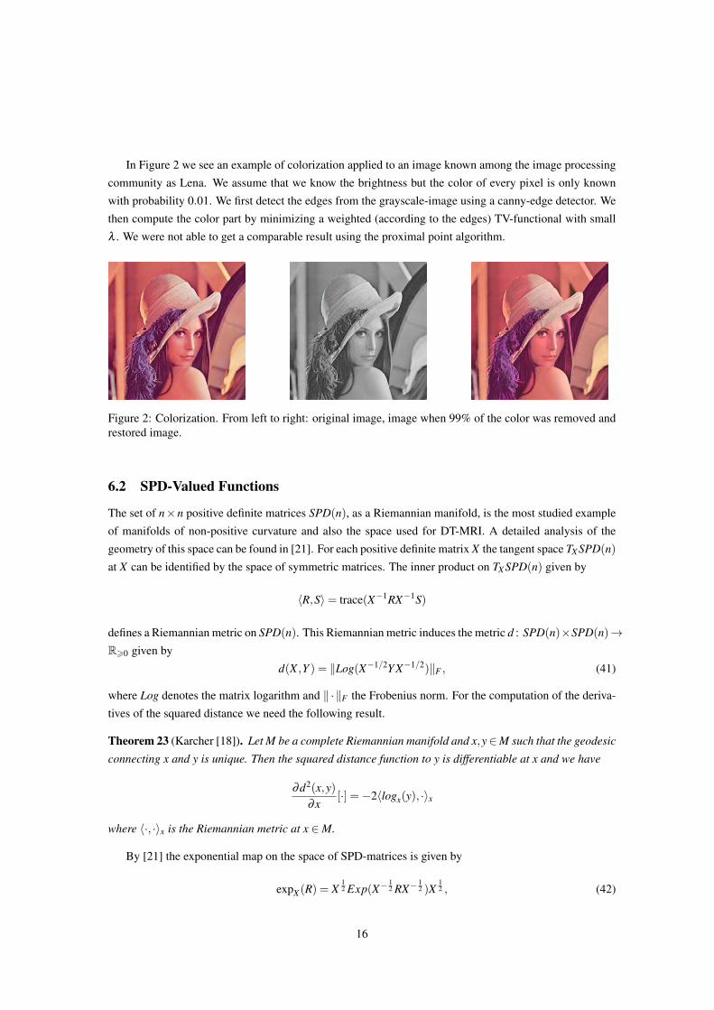
In Figure 2 we see an example of colorization applied to an image known among the image processing

community as Lena. We assume that we know the brightness but the color of every pixel is only known

with probability 0.01. We first detect the edges from the grayscale-image using a canny-edge detector. We

then compute the color part by minimizing a weighted (according to the edges) TV-functional with small

λ . We were not able to get a comparable result using the proximal point algorithm.

Figure 2: Colorization. From left to right: original image, image when 99% of the color was removed and

restored image.

6.2 SPD-Valued Functions

The set of n×n positive definite matrices SPD(n), as a Riemannian manifold, is the most studied example

of manifolds of non-positive curvature and also the space used for DT-MRI. A detailed analysis of the

geometry of this space can be found in [21]. For each positive definite matrix X the tangent space TX SPD(n)

at X can be identified by the space of symmetric matrices. The inner product on TX SPD(n) given by

〈R,S〉= trace(X−1RX−1S)

defines a Riemannian metric on SPD(n). This Riemannian metric induces the metric d : SPD(n)×SPD(n)→R>0 given by

d(X ,Y ) = ‖Log(X−1/2Y X−1/2)‖F , (41)

where Log denotes the matrix logarithm and ‖ · ‖F the Frobenius norm. For the computation of the deriva-

tives of the squared distance we need the following result.

Theorem 23 (Karcher [18]). Let M be a complete Riemannian manifold and x,y∈M such that the geodesic

connecting x and y is unique. Then the squared distance function to y is differentiable at x and we have

∂d2(x,y)

∂x[·] =−2〈logx(y), ·〉x

where 〈·, ·〉x is the Riemannian metric at x ∈ M.

By [21] the exponential map on the space of SPD-matrices is given by

expX (R) = X12 Exp(X− 1

2 RX− 12 )X

12 , (42)

16

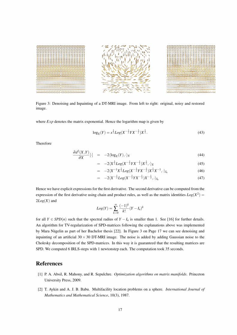
Figure 3: Denoising and Inpainting of a DT-MRI image. From left to right: original, noisy and restored

image.

where Exp denotes the matrix exponential. Hence the logarithm map is given by

logX (Y ) = x12 Log(X− 1

2 Y X− 12 )X

12 . (43)

Therefore

∂d2(X ,Y )

∂X[·] = −2〈logX (Y ), ·〉X (44)

= −2〈X 12 Log(X− 1

2 Y X− 12 )X

12 , ·〉X (45)

= −2〈X−1X12 Log(X− 1

2 Y X− 12 )X

12 X−1, ·〉In (46)

= −2〈X− 12 Log(X− 1

2 Y X− 12 )X− 1

2 , ·〉In (47)

Hence we have explicit expressions for the first derivative. The second derivative can be computed from the

expression of the first derivative using chain and product rules, as well as the matrix identities Log(X2) =

2Log(X) and

Log(Y ) =∞

∑k=0

(−1)k

k!(Y − In)

k

for all Y ∈ SPD(n) such that the spectral radius of Y − In is smaller than 1. See [16] for further details.

An algorithm for TV-regularization of SPD-matrices following the explanations above was implemented

by Mara Nagelin as part of her Bachelor thesis [22]. In Figure 3 on Page 17 we can see denoising and

inpainting of an artificial 30× 30 DT-MRI image. The noise is added by adding Gaussian noise to the

Cholesky decomposition of the SPD-matrices. In this way it is guaranteed that the resulting matrices are

SPD. We computed 6 IRLS-steps with 1 newtonstep each. The computation took 35 seconds.

References

[1] P. A. Absil, R. Mahony, and R. Sepulchre. Optimization algorithms on matrix manifolds. Princeton

University Press, 2009.

[2] T. Aykin and A. J. B. Babu. Multifacility location problems on a sphere. International Journal of

Mathematics and Mathematical Science, 10(3), 1987.

17

[3] W. Ballmann. Lectures on spaces of nonpositive curvature, volume 25 of DMV Seminar. Birkhauser

Verlag, Basel, 1995.

[4] P. Blomgren and T. F. Chan. Color tv: Total variation methods for restoration of vector valued images.

Institute of Electrical and Electronics Engineers Transaction on Image Processing, 7:304–309, 1996.

[5] M. R. Bridson and A. Haefliger. Metric spaces of non-positive curvature. Springer-Verlag, 1999.

[6] M. Cavegn. Total variation regularization for geometric data. Master thesis, ETH Zurich, 2013.

[7] A. Chambolle. An algorithm for total variation minimization and applications. Journal of Mathemat-

ical Imaging and Vision, 20(1-2):89–97, 2004.

[8] A. Chambolle and P.-L. Lions. Image recovery via total variation minimization and related problems.

Numerische Mathematik, 76(2):167–188, 1997.

[9] T. F. Chan, G. H. Golub, and P. Mulet. A nonlinear primal-dual method for total variation-based

image restoration, 1995.

[10] T. F. Chan, S. H. Kang, and J. Shen. Total Variation Denoising and Enhancement of Color Images

Based on the CB and HSV Color Models . Journal of Visual Communication and Image Repre-

sentation, 12(4):422–435, 2001.

[11] O. Christiansen, T.-M. Lee, J. Lie, U. Sinha, and T. F. Chan. Total variation regularization of matrix-

valued images. Internation Journal of Biomedical Imaging, 2007.

[12] O. Coulon, D. C. Alexander, and S. R. Arridge. Diffusion tensor magnetic resonance image regular-

ization. Medical Image Analysis, 8(1):47–67, 2004.

[13] I. Daubechies, R. Devore, M. Fornasier, and C. S. Gunturk. Iteratively reweighted least squares

minimization for sparse recovery. Communications on Pure and Applied Mathematics, 2008.

[14] U. R. Dhar and J. R. Rao. Domain approximation method for solving multifacility location problems

on a sphere. The Journal of the Operational Research Society, 33(7):pp. 639–645, 1982.

[15] M. Fornasier. Theoretical Foundations and Numerical Methods for Sparse Recovery. De Gruyter,

2010.

[16] P. Grohs, M. Sprecher, and T. Yu. Scattered manifold-valued data approximation. Technical Re-

port 23, Seminar for Applied Mathematics, ETH Zurich, Switzerland, 2014.

[17] S. H. Kang and R. March. Variational models for image colorization via chromaticity and brightness

decomposition. Image Processing, Institute of Electrical and Electronics Engineers Transactions on,

16(9):2251–2261, 2007.

[18] H. Karcher. Riemannian center of mass and mollifier smoothing. Communications on Pure and

Applied Mathematics, 30(5):509–541, 1977.

[19] J. Lellmann, E. Strekalovskiy, S. Koetter, and D. Cremers. Total Variation Regularization for Func-

tions with Values in a Manifold. Institute of Electrical and Electronics Engineers International Con-

ference on Computer Vision, 0:2944–2951, 2013.

18

[20] J. Milnor. Topology From the Differentiable Viewpoint. Princeton University Press, 1976.

[21] M. Moakher and M. Zeraı. The riemannian geometry of the space of positive-definite matrices and

its application to the regularization of positive-definite matrix-valued data. Journal of Mathematical

Imaging and Vision, 40(2):171–187, 2011.

[22] M. Nagelin. Total variation regularization for tensor valued images. Bachelor thesis, ETH Zurich,

2014.

[23] P. Perona. Orientation diffusions. Image Processing, Biomedical Imaging Transactions on, 7(3):457–

467, 1998.

[24] M.J.D. Powell. On search directions for minimization algorithms. Mathematical Programming,

4(1):193–201, 1973.

[25] P. Rodrıguez and B. Wohlberg. An iteratively reweighted norm algorithm for total variation regular-

ization. Signals, Systems and Computers, 2006.

[26] L. Rudin and V. Caselles. Image recovery via multiscale total variation. In in Proceedings of the

Second European Conference on Image Processing, pages 15–7, 1998.

[27] L. I. Rudin, S. Osher, and E. Fatemi. Nonlinear total variation based noise removal algorithms.

Physica D, 60(1-4):259–268, November 1992.

[28] N. Sochen, R. Kimmel, and R. Malladi. A general framework for low level vision. Institute of

Electrical and Electronics Engineers Transaction on Image Processing, 7:310–318, 1997.

[29] Karl-Theodor Sturm. Probability measures on metric spaces of nonpositive curvature. In Heat kernels

and analysis on manifolds, graphs, and metric spaces (Paris, 2002), volume 338 of Contemporary

Mathematics, pages 357–390. American Mathematical Society, Providence, RI, 2003.

[30] B. Tang, G. Sapiro, and V. Caselles. Color image enhancement via chromaticity diffusion. Institute

of Electrical and Electronics Engineers Transactions on Image Processing, 10:701–707, 2002.

[31] A. Weinmann, L. Demaret, and M. Storath. Total variation regularization for manifold-valued data.

Computing Research Repository, 2013.

[32] Li Y.-f. and Feng X.-c. The split bregman method for l1 projection problems. Chinese Journal of

Electronics, 38(11):2471, 2010.

[33] J. Yang, Y. Zhang, and W. Yin. A Fast Alternating Direction Method for TVL1-L2 Signal Reconstruc-

tion From Partial Fourier Data. Institute of Electrical and Electronics Engineers Journal of Selected

Topics in Signal Processing, 4(2):288–297, 2010.

19

Recent Research Reports

Nr. Authors/Title

2014-29 H. Rauhut and Ch. SchwabCompressive sensing Petrov-Galerkin approximation of high-dimensional parametricoperator equations

2014-30 M. HansenA new embedding result for Kondratiev spaces and application to adaptiveapproximation of elliptic PDEs

2014-31 F. Mueller and Ch. SchwabFinite elements with mesh refinement for elastic wave propagation in polygons

2014-32 R. Casagrande and C. Winkelmann and R. Hiptmair and J. OstrowskiDG Treatment of Non-Conforming Interfaces in 3D Curl-Curl Problems

2014-33 U. Fjordholm and R. Kappeli and S. Mishra and E. TadmorConstruction of approximate entropy measure valued solutions for systems ofconservation laws.

2014-34 S. Lanthaler and S. MishraComputation of measure valued solutions for the incompressible Euler equations.

2014-35 P. Grohs and A. ObermeierRidgelet Methods for Linear Transport Equations

2014-36 P. Chen and Ch. SchwabSparse-Grid, Reduced-Basis Bayesian Inversion

2014-37 R. Kaeppeli and S. MishraWell-balanced schemes for gravitationally stratified media

2014-38 D. Schoetzau and Ch. SchwabExponential Convergence for hp-Version and Spectral Finite Element Methods forElliptic Problems in Polyhedra