log-penalized least squares, iteratively reweighted lasso, and

Emory University Department of Biostatistics and Bioinformatics Technical Reports

Log-Penalized Least Squares, Iteratively Reweighted Lasso,

and Variable Selection for Censored Lifetime Medical Cost

Brent A. Johnson*

Department of Biostatistics and Bioinformatics, Emory University ([email protected])

Qi Long

Department of Biostatistics and Bioinformatics, Emory University

Yijian Huang

Department of Biostatistics and Bioinformatics, Emory University

Kari Chansky

The Fred Hutchinson Cancer Research Center

Mary Redman

The Fred Hutchinson Cancer Research Center

Technical Report 2012-02

December 2012

Department of Biostatistics and Bioinformatics

Rollins School of Public Health

1518 Clifton Road, N.E.

Emory University

Atlanta, Georgia 30322

Vol. 0 (2012) 1–24DOI: 10.1214/154957804100000000

Log-Penalized Least Squares, Iteratively

Reweighted Lasso, and Variable

Selection for Censored Lifetime Medical

Cost

Brent A. Johnson∗ and Qi Long† and Yijian Huang

Department of Biostatistics and BioinformaticsRollins School of Public Health

Emory UniversityAtlanta GA 30307 USA

e-mail: [email protected]; [email protected]; [email protected]

Kari Chansky and Mary Redman

The Fred Hutchinson Cancer Research Center1100 Fairview Ave N

PO Box 19024Seattle WA 98109, USA

e-mail: [email protected]; [email protected]

Abstract: Penalized least squares is a ubiquitous tool in statistics andits application are well-documented. Numerous investigators have investi-gated the tradeoffs between ℓ1-regularization versus non-concave penalties,the latter resulting in a sparser solution, smaller false positive rate andsmaller prediction error when the signal-to-noise ratio is large. Authorslater proposed one-step, convex approximations to non-concave penaltiesto avoid thorny numerical instabilibities and showed that these approx-imations possessed the same asymptotic properties. Here, we propogatelog-penalized least squares and a better numerical algorithm to computethe estimate. The algorithm is based on iteratively reweighted lasso, can beextended to any penalized likelihood problem, and can accommodate smallor large data sets. Our numerical studies suggest that log-penalized leastsquares is as good and often better than other leading estimators when thesignal-to-noise ratio is large.

Our substantive objective is to identify factors associated with censoredmedical cost, an important problem for patients and providers as well aslegislators at the state and national level. Direct application of estimatorsfor both uncensored and survival data lead to inconsistent estimation, ingeneral, and result in spurious conclusions from the data. In this paper, wepropose a new family of regularized estimators for lifetime censored medicalcost through an extension of penalized estimating functions. Then, we showthat a version of our estimator may be written as the minimizer of a convexsurrogate loss function. We investigate the operating characterisics of theseprocedures through simulation studies and application to lifetime medicalcost data due to nonsmall cell lung cancer from the Southwest OncologyGroup Protocol 9509.

∗Supported in part by the National Institutes of Health grant P30 AI050409†Supported in part by the National Institutes of Health PHS grant UL1 RR025008

1

imsart-generic ver. 2012/04/10 file: markvs_techrpt_2012.tex date: December 10, 2012

B. A. Johnson et al./Log-Penalized Regression 2

Keywords and phrases: Dependent censoring, Marked point process,Regularization, Survival analysis

.

1. Introduction

The federal government, insurance agencies and insured individuals all have aninterest in knowing what factors are associated with increased medical cost.If medical expenditures could be projected reliably, individuals could use suchresource for planning purposes. This is our principal motivation in modelingcensored lifetime medical cost as a function of clinical predictors in a South-west Oncology Group (SWOG) clinical trial for treatment of nonsmall cell lungcancer. Modeling medical costs is also important in econometrics and healthpolicy and management. Insurers use statistical models to predict cost and setinsurance premiums based on subject characteristics. In March 2010, PresidentBarack Obama signed into law, the Affordable Care Act, which stated as oneof its objectives, “lower[ing] health care costs over the lifetime” of an individual(www.whitehouse.gov). Thus, modeling medical costs is an important problemin health policy, econometrics, and subject-level cost management.

Regularized estimation will serve as the cornerstone of our variable selectionprocedure in Section 2. Because there has been so much theoretical and nu-merical work in this arena over the past several years, a brief summary of therelevant literature and how the current paper fits into that literature is imper-ative. To this end, we begin with estimation in the linear regression model foran uncensored outcome Y ,

Y = z1β1 + z2β2 + · · ·+ zdβd + εY (1.1)

where z = (z1, . . . , zd)T are regressors, β = (β1, . . . , βd)

T are regression coeffi-cients and εY are mean-zero stochastic errors. The observed data are Yi, zini=1

and assumed to be a random sample of size n from model (1.1). Coefficient es-timation by subset selection may be written as the ℓ0-optimization,

minβ∈Rd

1

2‖Y − Zβ‖2ℓ2 + λ‖β‖ℓ0 , (1.2)

where ℓ0-norm is the number of non-zero elements of the coefficient vector β.Tibshirani’s (1996) least absolute shrinkage and selection operator (lasso) isthe tightest convex relaxation of (1.2) and the ℓ1-regularized analog of (1.2).However, it is known that lasso has a tendency to overfit (Meinshausen andBuhlmann, 2006; Zhao and Yu, 2006) and shrink coefficient estimates too stronglytoward zero when the signal-to-noise ratio is large (Fan and Li, 2001; Zou, 2006;Meinshausen and Buhlmann, 2006; Zhao and Yu, 2006). Fan and Li (2001) werethe first to propose non-concave penalized least squares estimation through theirsmoothly clipped absolute deviation (scad) penalty and showed that this newestimator was root-n consistent, would select the correct submodel with highprobability, and converged to the same asymptotic distribution as if one had



known the correct submodel a priori. Zou (2006) showed that if one weightedthe ℓ1-regularization in Tibshirani’s lasso with weights proportional to the in-verse of the absolute value of the regression coefficients from a preliminary leastsquares fit, then the weighted lasso (i.e. the adaptive lasso) could achieve thesame asymptotic properties as scad. But, unlike scad, adaptive lasso was a con-vex optimization problem, could make use of existing algorithms to solve theoriginal lasso problem, and may be preferable on numerical grounds. Althoughthese two methods are popular in the statistics literature, there exist otherlesser-known, less mature methods with the same asymptotic properties butbetter finite sample properties.

The focus of this paper is simultaneous coefficient estimation and variableselection via log-penalized least squares, i.e.

minβ∈Rd

1

2‖Y − Zβ‖2ℓ2 + λ

d∑

j=1

log(|βj |). (1.3)

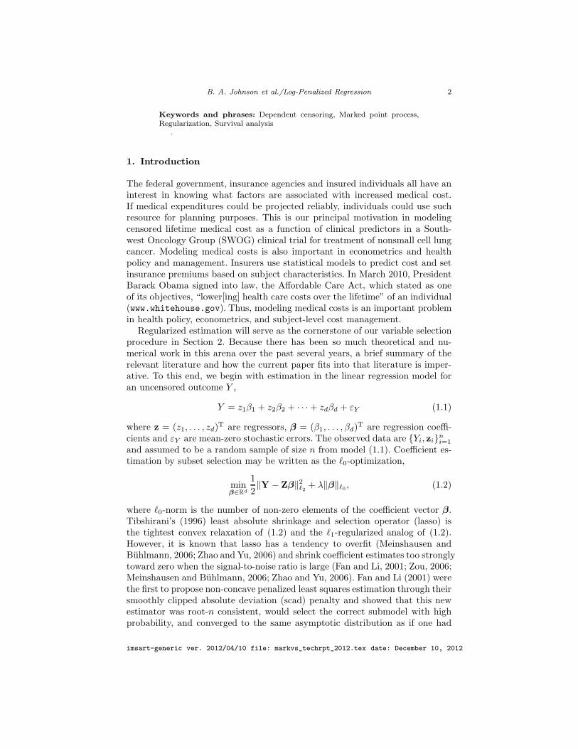
Log-penalized regression has received scant attention in the statistics literatureeven though it results in a sparse solution and can be adapted for variable selec-tion. Logarithmic penalty is related to the smoothly clipped absolute deviation(scad; Fan and Li, 2001) in that they are both non-concave penalty functionsand offer better approximations to cardinality than does the ℓ1-norm. In Fig-ure 1, we illustrate the scad and logarithmic penalty. Compared with scad, log-

−1.0 −0.5 0.0 0.5 1.0

0.0

0.4

0.8

Pe

na

lty(β

)

β

Scad

−1.0 −0.5 0.0 0.5 1.0

0.0

0.4

0.8

Pe

na

lty(β

)

β

Log

Fig 1. Common penalty functions and their proximity to cardinality. Scad (solid blue) penaltyin the left panel and logarithmic (solid blue) penalty in the right panel. Cardinality is repre-sented by a solid vertical line.

arithm penalty offers a closer approximation to cardinality. Then, heuristically,



one might believe that logarithmic penalty also offers a closer approximation tosubset selection.

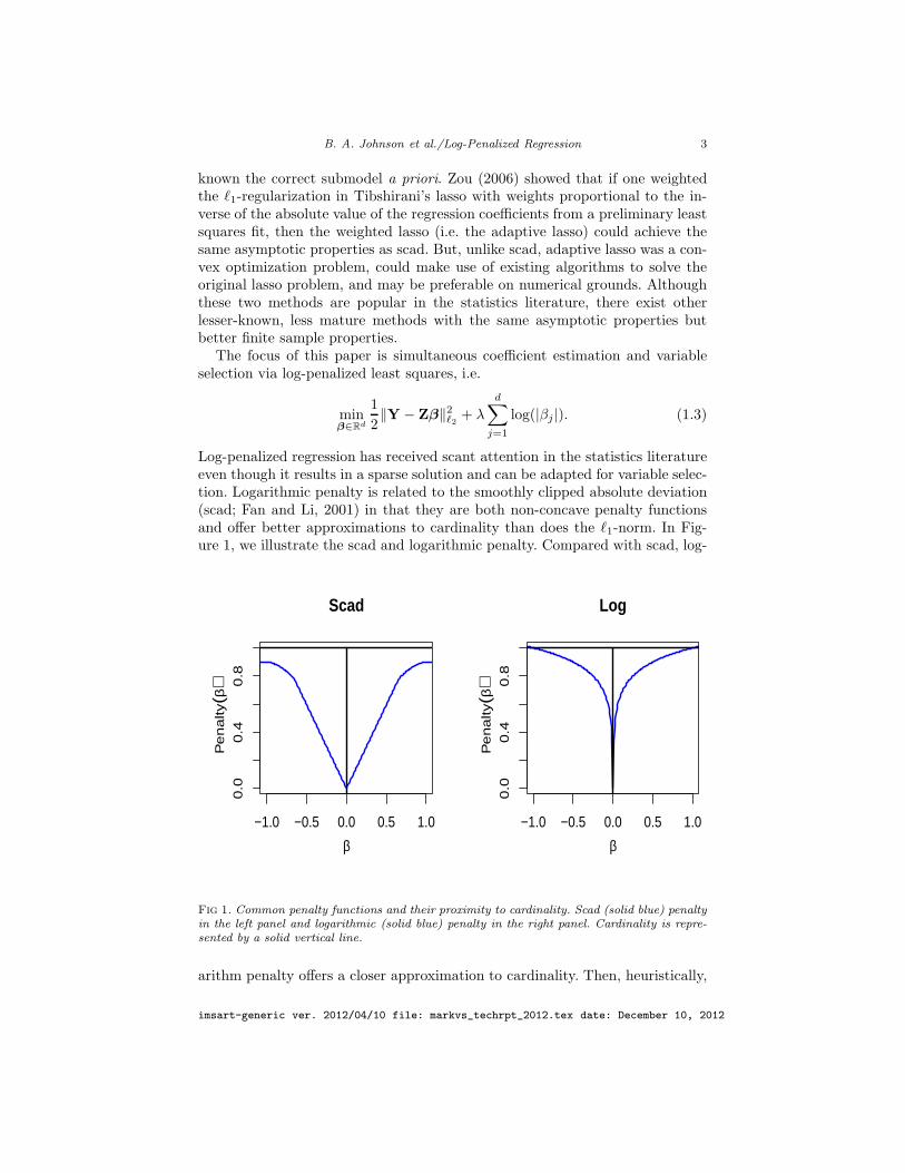
By now, a couple authors have discussed asymptotic properties of log-penalizedregression estimators. Johnson, Lin and Zeng (2008) discuss log-penalized re-gression in the context of penalized estimating functions and show that it, alongwith several other common penalty functions, possess an oracle property. Zouand Li (2008) show that a one-step approximation to the log-penalized esti-mator is Zou’s (2006) adaptive lasso estimator which also possesses an oracleproperty. Despite optimal asymptotic properties, statisticians have found mini-mizing (1.3) awkward and tricky. Zou and Li (2008) offer some insight into theoperational difficulty of logarithmic penalty, ℓ0.01-penalty, and bridge penalty.In Figure 2, adapted from Zou and Li (2008), we see that logarithmic penaltyresults in a discontinous thresholding rule for orthonormal designs. Fan and

−10 −5 0 5 10

−1

0−

50

51

0

Scad

β−10 −5 0 5 10

−1

0−

50

51

0Log

β−10 −5 0 5 10

−1

0−

50

51

0

Ada. Lasso

β

Fig 2. Thresholding rules for scad, log, and adaptive lasso penalty functions.

Li (2001) recommend avoiding penalty functions, e.g. logarithmic penatly, thatbreak the following rule (their rule no. 3) of a “good” penalty function:

“3. Continuity: The resulting estimator is continuous in data z to avoid instabilityin model prediction.” (Fan and Li, 2001, p. 1349)

From Figure 2, it is clear that logarithmic penalty results in a discontinuousthresholding rule whereas scad and adaptive lasso result in continuous thresh-olding rules. In addition, bridge penalty results in a discontinous thresholdingrule for any power less than one (cf. Fan and Li, 2001). The impetus of ruleno. 3 is numerical inaccuracy near the boundary constraints so that when oneapplies the “usual” numerical tricks (Tibshirani, 1996; Fan and Li, 2001; Hunterand Li, 2005; Zou and Li, 2008) to logarithmic or bridge penalty, the quadraticor linear approximation is either too crude or the algorithm simply does notconverge (i.e. infinite oscillation, multiple roots).



In this paper, we extend a recent algorithm proposed by authors in the com-pressed sensing and signal processing literature (Candes, Wakin and Boyd, 2008;Daubechies et al., 2009; Gasso, Rakotomamonjy and Canu, 2009) that can beused to overcome the challenges in minizing (1.3) and open the door to othercomplex optimization problems. The numerical algorithm amounts to iterativelyreweighted lasso (Gasso, Rakotomamonjy and Canu, 2009) and the techniquecan be used to manipulate any discontinuous thresholding rule with a singularityat the origin into a stable variable selection procedure. This recent developmentdebunks the myth in statistics that penalties resulting in discontinuous thresh-olding rules ought to be avoided.

Our contributions to the literature are three-fold: (a) to advocate and pro-pogate an iteratively reweighted lasso procedure (Gasso, Rakotomamonjy andCanu, 2009) for log-penalized regression in large- or small-scale problems, (b)to extend this technique from penalized least squares to a semi-parametric es-timator for a problem with induced dependent censoring, and (c) to apply thetechnique to censored lifetime medical cost data from SWOG 9509. Lifetimemedical cost is an example of a marked outcome, an endpoint observed at thetime of failure but not when the failure event is censored. Although the sta-tistical analysis of censored medical cost has received substantial attention inthe literature (cf. Lin, Feuer and Wax, 1997; Huang and Louis, 1998; Bang andTsiatis, 2000; Huang, 2002; Jain and Strawderman, 2002; Huang and Lovato,2002), there is only one other paper on variable selection for censored medicalcost data. Approximately one decade ago, Jain and Strawderman (2002) mod-eled the log hazard function of censored lifetime cost as a function of covariatesusing piecewise linear splines and their tensor products. They employed inverseweighted estimating equations to account for the induced informative censoringand introduced a stepwise deletion procedure to add or delete basis functionsin their model so as to improve the finite sample properties of their estima-tor. Here, rather than build on the inverse weighting framework, our family ofestimation procedures is built on the class of weighted logrank estimators viaHuang’s (2002) calibration regression for censored lifetime medical cost. In ad-dition, the family of ℓ1-regularized coefficient estimators proposed here is quitedifferent than stepwise deletion.

We perform simulation studies in Section 5 to evaluate the perfomance ofseveral related procedures in the n > d paradigm, which is the paradigm ofinterest for our censored medical cost application. Because our literature reviewis not specific to censored data and we report results from simulation studiesfor both censored and uncensored data, our conclusions may appeal an audiencebeyond the specific medical cost application. The conclusions are as follows:

• Iteratively reweighted ℓ1 minimization is different than one-step approx-imations and our numerical studies indicate that estimates computed byiteratively reweighting leads to a smaller false positive error rate and asmaller predition error;

• Even when the asymptotic distribution among “oracle” procedures is thesame, not all such procedures perform equally well in finite samples. We



found that bridge and logarithmic penalty performed somewhat betterthan scad and adaptive lasso among penalized least squares estimatorsin complete, uncensored data simulations. Our findings in the n > dparadigm agree with and complement other numerical studies in the sig-nal processing and compressed sensing literature for the high-dimensionalcase (cf. Candes, Wakin and Boyd, 2008; Daubechies et al., 2009; Gasso,Rakotomamonjy and Canu, 2009);

• Weighting ℓ1 minimizers are powerful tools that many authors have ex-plored before us, but some of these authors have taken unfortunate turnsleading to suboptimal weights. We observed that when the optimal weightsare used, the weighted lasso performs as well as or better than the Oracle,on average. Poor weighting schemes can lead to estimators that performworse than the unweighted ℓ1-type estimator and, hence, have an unde-sirable effect;

• In the presense of marked outcome data, the trends were generally thesame as in the uncensored data case but with bridge regression (i.e. ℓ0.5-regression) performing slightly better than its competitors.

2. Methods for Censored Lifetime Medical Cost

2.1. Notation

For i = 1, . . . , n, let Yi be a mark variable of interest observed at the log-transformed event time Ti, and zi = (zi1, . . . , zid)

T is a d-vector of independentregressors. Write the joint regression model,

Yi =

d∑

j=1

zijβj + εY,i, Ti =

d∑

j=1

zijϑj + εT,i, (2.1)

where the unknown parameters include the regression coefficients on the markscale, β = (β1, . . . , βd)

T, as well as regression coefficients on the time scale,ϑ = (ϑ1, . . . , ϑd)

T. We assume that the bivariate random error vector εi =(εY,i, εT,i)

T is independent and identically distributed according to an unspec-ified bivariate distribution function. In mark variable regression, the observeddata are Yi, Ti, δi, zini=1, where Yi = Yi · I(Ti ≤ Ci), Ti = min(Ti, Ci), δi =I(Ti ≤ Ci), for a random censoring variable Ci, e.g. administrative censoringat the end of clinical study. For some applications, if may be reasonable to as-sume that the mark Yi is linearly related to regressors exactly as it is written in(2.1). However, because of the right-skewed nature of patient medical cost data,we assert a loglinear relationship such that Yi in (2.1) pertains to transformedmedical cost on natural logarithmic scale.

2.2. Coefficient Estimation

Define the at-risk process Ri(u,ϑ) = I(Ti − zTi ϑ ≥ u) and counting process

NεTi (u,ϑ) = I(Ti − zTi ϑ ≤ u, δi = 1). Let ΛεT (·) be the cumulative baseline



hazard function of εT in (2.1). Following standard martingale theory, we havethat

M εTi (t) = NεT

i (t,ϑ)−∫ t

−∞

Ri(s,ϑ) dΛεT (s),

is a local martingale with respect to the filtration

Ft = σ

I(Ti − zTi ϑ ≤ u, δi = 1), I(Ti − zTi ϑ ≤ u, δi = 0),

Y · I(Ti − zTi ϑ ≤ u, δi = 1), zi, u ≤ t, i = 1, . . . , n

.

The filtration Ft contains all the survival information up to and including timet, and we can appeal to classic counting process theory (cf. Andersen et al.,1993) to construct a consistent estimator of the regression coefficient vector ϑ

on the time-scale. In particular, the usual weighted logrank estimating function(Tsiatis, 1990; Wei, Ying and Lin, 1990) for ϑ is

SεT (ϑ) =

n∑

i=1

∫ ∞

−∞

WεT (u,ϑ) zi − z(u,ϑ) dNεTi (u,ϑ),

whereWεY (t,ϑ) is a Ft-predictable, non-negative weight function and the weightedaverage of regressors, z(u,ϑ) =

∑j zjRj(u,ϑ)/

∑j Rj(u,ϑ). We define the

marked process as the product,

NεYi (t, θ) = NεT

i (t,ϑ)ψ(Yi − zTi β), (2.2)

where ψ(·) is a known continuous and strictly monotone (Huang, 2002). Thisleads to Huang’s estimator for β, that is, the solution to 0 = SεY (θ), where

SεY (θ) =n∑

i=1

∫ ∞

−∞

WεY (u, θ) zi − z(u,ϑ) dNεYi (u, θ). (2.3)

Note, that estimating function SεY (θ) in (2.3) looks very much like the weightedlogrank estimating function SεT (ϑ) but there are some important differences.First, the weight function WεY (u, θ) can be a function of the time- and mark-scale parameters. Second, the jump-size of the marked process NεY

i (u, θ) isstochastic unlike standard applications of counting process theory for survivalanalysis (cf. Kalbfleisch and Prentice, 2002). Thus, in general, solving 0 =SεY (θ) can be a difficult task numerically due to choice of weight functionsWεY and ψ.

2.3. Local Least Squares

To induce sparsity in coefficient estimation, one possible approach is to augmentthe estimating function SεY (θ) with a penalty function that imposes a jump



discontinuity at zero (cf. Fu, 2003; Johnson, Lin and Zeng, 2008). However, aparticular version of the score SεY (θ) will have better numerical properties.

In the special case where ψ(t) = t in (2.2) and WεY (u, θ) is not a function ofβ, the estimating function SεY (θ) simplifies significantly. Write the simplifiedthe weight function in (2.3) as WεY (u, θ) =WεY (u,ϑ), because we still assumethe weight function may depend on the time-scale coefficient vector ϑ. In thiscase, solving the estimating equation, 0 = SεY (θ), is equivalent to solving thelinear system,

M(ϑ)β = v(ϑ), (2.4)

where

v(ϑ) =n∑

i=1

∫ ∞

−∞

WεY (u,ϑ)Yi zi − z(u,ϑ) dNεTi (u,ϑ),

M(ϑ) =

n∑

i=1

∫ ∞

−∞

WεY (u,ϑ) zi − z(u,ϑ)⊗2dNεT

i (u,ϑ),

where v⊗2 = vvT. Indeed, Huang’s (2002) original estimator is defined:

βFull = M(ϑ∗)−1v(ϑ∗),

where ϑ∗ is a p-dimensional estimate of the time-scale regression coefficientsϑ. In Huang (2002) and in this paper, ϑ∗ is assumed to be root-n consistentand computed as the solution to the weighted log rank estimating equationson the time-scale, 0 = SεT (ϑ); see Section 6 for comments on estimation inhigh dimensions. To define our regularized estimator, we rewrite the solutionto the linear system (2.4) as the minimum of squared errors. Define the vectorV(ϑ) = AT(ϑ)−1v(ϑ) where A(ϑ) is the Choleski decomposition of M(ϑ),i.e. AT(ϑ)A(ϑ) = M(ϑ). Then, our log-penalized coefficient estimator isdefined as the minimizer

β = minβ∈Rd

L(β,ϑ∗) + λ

d∑

j=1

log(|βj |), (2.5)

with surrogate loss function,

L(β,ϑ∗) =1

2V(ϑ∗)−A(ϑ∗)βT V(ϑ∗)−A(ϑ∗)β ,

The asymptotic properties of the log-penalized estimator β are described in aWeb Appendix. In Section 3, we show how to effectively solve for logarithmicpenalty through iteratively reweighted lasso.

3. Computational Methods

3.1. Fundamental Tools from Compressed Sensing

Over the last three decades, there has been a largely independent and parallelinterest among engineers, computer scientists, and mathematicians in solving



an underdetermined linear systems of equations, say,

Zβ = Y, (3.1)

where Y ∈ Rn, Z is an n×dmatrix with n < d and β ∈ R

d are parameters to beestimated. Because the system is underdetermined, there are infintely solutionsthat satisfy (3.1). Assuming that the true vector of unknowns β is itself sparseleads one to believe the ℓ1 minimization approach could be a reasonable solutionto (3.1), say

minβ∈Rd

‖β‖ℓ1 s.t. Y = Zβ. (3.2)

Recently, Daubechies et al. (2009) outlined the historical development of theℓ1 minimization solution to (3.1) and traced the earliest applications back tothe late-1970s although the first theoretical justification did not come untilthe late-1980s. Recently, Candes, Wakin and Boyd (2008) offered the followingimprovement:

minβ∈Rd

‖Wβ‖ℓ1 s.t. Y = Zβ, (3.3)

where W = diagw1, . . . , wd and

wj =

1|β0j|

, j ∈ A,∞, j ∈ Ac,

(3.4)

where the active set is defined A = j|β0j 6= 0, j = 1, . . . , d. However, becausethe optimal weights are unknown, (3.3) cannot be solved directly. So, Candes,Wakin and Boyd (2008) offered the following approximation. By adding a smallerror, one can rewrite the optimization problem in (3.3) as

minβ∈Rd

d∑

j=1

log(|βj |+ ǫ) s.t. Y = Zβ,

which can then be iteratively solved. Given current iterates β(k−1)j , at the k-th

iteration, one solves the weighted ℓ1 minimization,

minβ∈Rd

d∑

j=1

(1

|β(k−1)j |+ ǫ

)|βj | s.t. Y = Zβ. (3.5)

The rationale behind (3.5) is that because the logarithm function is concave,one can improve on a guess to the solution by locally minimizing a linearizedfunction centered at the current guess and repeating the process (Candes, Wakinand Boyd, 2008). This is the essence of MM algorithms which have a longhistory of application in computer science, statistics and applied mathematics.In a similar spirit, Daubechies et al. (2009) suggested iteratively reweighting ℓ2minimization for sparse recovery.



3.2. Iteratively Reweighted Lasso

Now, we apply the principles embodied in Candes, Wakin and Boyd (2008) topenalized least squares. Gasso, Rakotomamonjy and Canu (2009) published avariation of this algorithm first under the title of “DC programming,” where“DC” stands for difference in convex functions. Rewrite the log-penalized esti-mator in (1.3) as the perturbed expression

minβ∈Rd

1

2‖Y − Zβ‖2ℓ2 + λ

d∑

j=1

log(|βj |+ ǫ)

. (3.6)

Then, taking a first-order Taylor-series approximation of the logarithm penaltyabout the current value βj = β∗

j , we obtain the over-approximation of (3.6),

minβ∈Rd

1

2‖Y − Zβ‖2ℓ2 + λ

d∑

j=1

(1

|β∗j |+ ǫ

)|βj |

. (3.7)

Note, the linear approximation in (3.7) is analogous to one proposed in Zou andLi (2008) except that Zou and Li (2008) did not make use of the perturbation ǫand they argued strongly in favor of a one-step approximation. Instead, we offerthe following algorithm to generate the entire coefficient path for log-penalizedleast squares. Assume all the covariates have been standardized to have meanzero and unit variance. Without loss of generality, the span of regularizationparameters is λmin = λ0 < · · · < λL = λmax, for l = 0, . . . , L (cf. Friedmanet al., 2007).

Algorithm 1.

(A.1) Start with λmax = max1≤j≤d |zTj Y|/n. Set l = L and β(l) = 0.OUTER LOOP:

(B.0) Set t = 0 and β[0]

= β(l);

(B.1) Increment t = t+ 1 and β[t+1]

= β[t];

(B.2) Update the weights: wj = 1/|(β[t]j + ǫ), j = 1, . . . , d;

INNER LOOP: Solve the Karush-Kuhn-Tucker (KKT) conditions forfixed wj :

zTj (Y − Zβ)− λlwjsgn(βj) = 0, if j ∈ A,|zTj (Y − Zβ)| < λlwj , if j /∈ A,

(B.3) Goto step (B.1);

(B.4) Repeat steps (B.1)–(B.3) until ‖β[t+1] − β[t]‖ℓ∞ < τ . The estimate

β(l) is the limit point of the outer loop, β[∞]

;



(A.2) Decrement l = l − 1 and λl = λl−1. Return to (B.0) using β(l) as awarm start.

In small-scale problems where n > d, we set λmin = 0. However, when n < d,one attains the saturated model long before the regularization parameter reacheszero. In this case, we suggest λmin = 10−4λmax (cf. Friedman et al., 2007). Weused τ = ǫ = 10−3 as in Gasso, Rakotomamonjy and Canu (2009).

Remark 1. Algorithm 1 is very much like majorization-minorization (MM) al-gorithms, a generalization of EM algorithms for missing data problems and astaple of modern statistical computation. Hunter and Li (2005) were the first toadvocate MM algorithms for variable selection when n > d while Candes, Wakinand Boyd (2008) was the first to suggeset an MM algorithm for the logarithmicpenalty regardless of the dimension of d relative to the sample size n (see also,Gasso, Rakotomamonjy and Canu, 2009; Daubechies et al., 2009). A subtle butimportant point is to notice how Algorithm 1 differs from the algorithm de-scribed in Hunter and Li (2005). The use of MM algorithms in Hunter and Li(2005) is to justify a quadratic over-approximation to penalty functions withsingularities at the origin. In the inner loop of Algorithm 1, we avoid such ap-proximation by solving the KKT conditions precisely and efficiently (Osborne,Presnell and Turlach, 2000; Efron et al., 2004). Our use of MM algorithms inAlgorithm 1 is to justify the local linear approximation to logarithmic penaltyin the outer loop.

Remark 2. Local linear approximations to logarithmic and bridge penalty werealso proposed by Zou and Li (2008). Algorithm 1 differs from that proposed byZou and Li (2008) in that it constructs the entire coefficient path, even whenn < d, whereas the procedure by Zou and Li (2008) computes the coefficient es-timates for a fixed regularization parameter λ starting with a root-n consistentestimator of the true coefficient β0 at the intial step. Moreover, even with thesame intial estimate, the limit point from Algorithm 1 will differ from Zou andLi (2008) after one iteration;

Remark 3. In the more general case where n < d, we used coordinate-wise opti-mization (cf. Friedman et al., 2007) to compute the entire regularized coefficientpath via Algorithm 1. Gasso, Rakotomamonjy and Canu (2009) also suggestedthat one could adopt coordinate-wise optimization but, in the end, they set-tled on another algorithm. Our experience is that coordinate-wise optimizationworks well in practice and converges very quickly;

Remark 4. In the case of marked outcomes, Algorithm 1 may be applied usingthe pseudo-response vector V(ϑ∗) and pseudo-design matrix A(ϑ∗). All otheralgorithmic details remain unchanged.

Although there is no theory guaranteeing convergence of MM algorithms,Gasso, Rakotomamonjy and Canu (2009) showed convergence for penalty func-



tions that could be represented as a difference of two convex functions, a re-sult which applies to logarithmic and bridge penalty. We tested Algorithm 1in several simulated data sets for n > d and, in our experience, it always con-verged in these cases. Other authors (Candes, Wakin and Boyd, 2008; Gasso,Rakotomamonjy and Canu, 2009; Daubechies et al., 2009) have tested the high-dimensional log-penalized estimator and we refer the interested reader to else-where in the literature for a discussion of this topic.

3.3. Parameter Tuning

For tuning the regularization parameter in a least squares framework for uncen-sored outcome data, we used an ordinary BIC statistic,

BIC(λ) =1

n‖Y − Zβ‖2ℓ2 + log(n)d(λ),

where d(λ) is the number of non-zero coefficient estimates in β. For parametertuning in a marked outcome framework, we used a type of dispersion statistic.Let Sε(θ) = (STεY , S

TεT )

T and β be a regularized estimate as a result of theprocedure described in Algorithm 1. Then, under Conditions A-E in Huang(2002, Appendix), n−1/2

Sε(θ0) converges in distribution to a mean-zero, normalrandom variable with covariance Ω(θ0), with

Ω(θ) = limn→∞

1

n

n∑

i=1

∫ ∞

−∞

WεY (u, θ)ψ(Yi − zTi β)

WεT (u,ϑ)

⊗2

⊗[∑n

j=1 z⊗2j Rj(u,ϑ)∑n

j=1Rj(u,ϑ)− z(u,ϑ)⊗2

]dNεT

i (u,ϑ),

whereA⊗B is the kronecker product of matricesA andB. If we let Ω(θ) denote

the empirical estimator for Ω(θ) and θFull = (βT

Full,ϑT∗ )

T, then our dispersionstatistic is defined as

X(λ) = n−1

(SεY (β,ϑ∗)SεT (ϑ∗)

)T

Ω−1

(θFull)

(SεY (β,ϑ∗)SεT (ϑ∗)

),

which, under suitable regularity assumptions (cf. Wei, Ying and Lin, 1990),X(λ) follows a χ2 distribution with degrees of freedom equal to the number of

non-zero coefficient estimates in (βλ,ϑ∗). Then, an BIC-type criterion can bedefined

BIC(λ) = X(λ) + log(n)d(λ),

where d(λ) is an estimate of the degrees of freedom for the fitted model; here,

we approximate d(λ) with the cardinality of the estimated active set on themark-scale. We define an analogous AIC-type criterion by substituting log(n)on the right-hand side of the above expression with two. We note that Jain andStrawderman (2002) define a similar statistic to X(λ) in their stepwise deletionprocedure for modeling the hazard of censored medical cost.



4. Analysis of the SWOG 9509 Data

The randomized Southwest Oncology Group (SWOG) 9509 trial was designed toinvestigate Paclitaxel plus Carboplatin versus Vinorelbine plus Cisplatin thera-pies in untreated patients with advanced nonsmall cell lung cancer. The primarystudy endpoint was survival time (Kelly et al., 2001) and subsequent secondaryanalyses considered lifetime medical costs (Huang and Lovato, 2002; Huang,2002) For each of 408 eligible study participants, the “lifetime medical cost”endpoint was computed from resource utilization metrics, including medica-tions, medical procedures, different treatments on- and off-protocol, and daysspent in the outpatient or inpatient clinic. The cost incurred for each type ofresource used was computed using national databases and were standardized to1998 US dollars (Huang, 2002). Resource utilization was measured at 3, 6, 12,18, and 24 month clinic visits. Both time and cost are modeled on the naturallogarithmic scale.

We considered 18 baseline variables as main effects in the joint regressionmodel (2.1). The regressors are treatment arm (trt, 1=Paclitaxel plus Carbo-platin, else 0), gender (sex), progression status (progstat), SWOG performancestatus (ps), clinical stage (stage), IIIB by pleural effusion, weight (kg), height(cm), creatinine (creat), albumin (g/dl), calcium (mg/dl), serum lactate dehy-drogenase (ldh, U/l), alkaline phosphatase (alkptase), bilirubin (mg/dl), whiteblood cell count (wbc, cells/microliter), platelet count (platelet, cells/microliter),hemoglobin level (hgb, g/dl), and age (years). Serum lactate dehydrogenase(ldh), alkaline phosphatase (alkptase), and bilirubin are all derived binary ran-dom variables, with one indicating that the patient’s measurement exceeded theupper limit of normal (ULN).

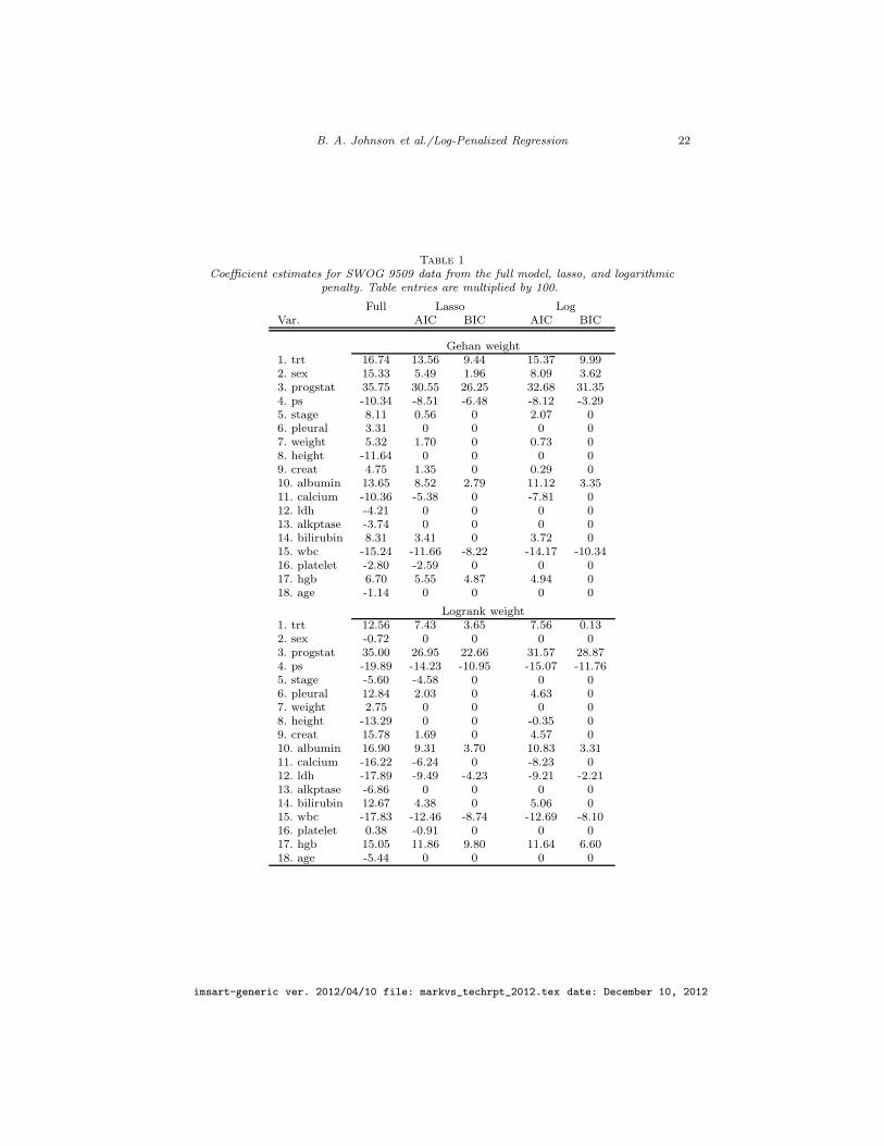
The sample size of our cost data was 398 participants and excluded 10 studyparticipants with insufficient documentation. This cost data set was mergedwith the data set of baseline variables. Then, we excluded all those patientsmissing any of the 18 covariates. This led to a final sample size of n = 343.As a final step of preprocessing, each of 18 baseline variables was standardizedto have mean zero and unit variance. The scale of the coefficients has no effecton model selection but facilitates displaying coefficient estimates for regressorswith measurement scales of varying order. The model selection procedure wasperformed for each of the Gehan and logrank weight function, with the sameweight function used in the time- and mark-scale score function. The results ofour model selection procedures are presented in Table 1.

The results in Table 1 lead to several interesting findings. First, the selectedvariables in the Gehan and logrank weights across lasso and log regularizations,generally agree although the magnitude of the coefficients in the active setsdiffer. The seven strongest predictors are treatment, progression status, SWOGperformance score, albumin level, lactate dehydrogenase, white blood cell count,and hemoglobin level. No fewer than five variables are selected by AIC but ig-nored by BIC using the same weight-penalty combination. Not surprisingly, wefind that progression status is the most informative predictor of higher medicalcost followed by white blood cell count. It is somewhat interesting to observe



how treatment, an unimportant variable on the time-scale as reported in Kellyet al. (2001), is moderately important on the cost-scale. The relative importanceof treatment differs by penalty and weight combination with Gehan weight in-flating its importance while log-penalty, logrank weight downweighting its im-portance. Nevertheless, the treatment variable underscores the dual roles thatcovariates play in joint models and that it is impossible to determine whichcovariates will be important on the cost-scale based solely on their prognosticvalue for the survival endpoint.

5. Simulation Studies

In our simulation studies, we presents results from nine regularized estimators,in addition to the full model estimator and the oracle. The nine regularizedestimators include familiar procedures such as lasso (Tibshirani, 1996), hardthresholding, scad (Fan and Li, 2001), bridge regression (ℓ0.5; Frank and Fried-man, 1993), and adaptive lasso (AL(Z); Zou, 2006). We also implement twoother versions of adaptive lasso. We include the adaptive lasso estimator by(AL(H); Huang, Ma and Zhang, 2008) which estimates fixed weights throughunivariate simple linear regressions for each covariate one-at-a-time. The opti-mal adaptive lasso (AL(Opt)) uses fixed weights wj = 1/(|β0j|+ ǫ). Finally, wealso include the multi-stage adaptive lasso (MSAL; Buhlmann and Meier, 2008)which iterateively reweights lasso but re-tunes the procedure at every stage.

5.1. Least Squares

In the first simulation set of simulations, we considered penalized least squaresestimators with no censoring whatsoever. The results from these studies allowus a cleaner comparison of various methods without artifacts of induced cen-soring and the marked outcome framework. We simulate outcomes Y accoringto a linear model with mean-zero normal errors and variance σ2. The covariatevector z is multivariate normal with mean zero, unit variance, and correlationcorr(zj , zk) = ρ|j−k|. The data are generated independently for n = 85 sam-ples. There are a total of d = 40 covariates, 22 of which have zero coefficientand no effect on outcome. The 18 non-zero coefficients are as follows: “3” inpositions 16, 17, 18; “2” in positions 6, 23, 24, 25, 32, 36; “3/2” in position 2;“1” in positions 1, 10, 11, 12, 27, 28, 33, 35. The following four statistics areused to compare the various procedures: ℓ2 error, median model error (ME),

ME = (β − β0)TE(zzT)(β − β0), average number of non-zero coefficients in-

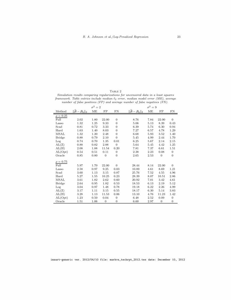
correctly set to zero (false negative), and average number of coefficients whosetrue value is zero but whose estimate is non-zero (false positive). Results from100 Monte Carlo are displayed in Table 2 for σ2 ∈ 2, 9 and ρ ∈ 0.25, 0.75.To compare with existing procedures in the literature based on MM algorithms(Hunter and Li, 2005), the algorithm for log-penalized least squares is also basedon a nested MM algorithm which computes estimator for a fixed regularization



parameter rather than the entire solution path. The range of regularization pa-rameters is 19 values in the interval [10−4, 1.6] × σ/

√n, where σ is the root

mean-squared error based on the full model. The values are computed on alog-scale and then transformed back; an identical set of values is used for scad,bridge, hard, log, MSAL, and all adaptive lasso estimators. All regularized es-timators were tuned using BIC criteria.

The results in Table 2 tell several interesting stories. First, logarithm penaltyhas the smallest false positive (FP) rate in three out of four scenarios amongestimators that can be computed using the observed data (thus, ruling outAL(Opt)). In the one instance where log does not have the smallest FP rate,bridge regression has the smallest FP error rate (i.e. when σ2 = 9 and ρ =0.75). In general, lasso has the smallest false negative (FN) rate meaning thatif lasso fails to include a variable in the final model, the corresponding trueregression coefficient is zero with high probability. Interestingly, when the dataare highly correlated, AL(H) has a false negative rate similar to lasso and a falsepositive worse than lasso. Hence, simple weighting schemes can adversely affectsthe performance of adaptive lasso. In some cases, AL(Z) has better predictionerror than bridge and logarithm penalty, but it comes at the expense of anunnecessarily complex model. In the situations we considered, MSAL and scadwere competitive with log, bridge, and AL(Z) but not the best performers.Finally, with optimal weights, we see that AL(Opt) has better prediction errorand ℓ2 error than the oracle and the FP and FN error rates are of the same orderas the oracle. Presumably, the prediction error of AL(Opt) is slightly better thanthe oracle because it retains one of two noise variables for improved finite sampleperformance and the slightly higher FP error rate is due to the perturbation.

5.2. Marked Outcomes

The second set of simulations is specific to the marked variable application.Here, we simulated data according the joint model

(YiTi

)= zTi

(β

ϑ

)+

(εY,iεT,i

),

where the errors (εY,i, εT,i) are bivariate normal with mean zero and covarianceΣ,

Σ = ΓRΓ =

(σεY 00 σεT

)(1 0.25

0.25 1

)(σεY 00 σεT

).

The design matrix and coefficients on the mark-scale are exactly as in Section 5.1except with a sample size of n = 150. The regression coefficients on the time-scale are ϑj = 0.5 for j = 1, . . . , d. In this setting, the censoring random variablewas independently simulated, Ci ∼ Un(0, 6). Then, the observed data is defined

as Ti = min(Ti, Ci), δi = I(Ti ≤ Ci), and Yi = δiYi + (1 − δi)(−100). The foursimulations represent weak (ρ = 0.25) and strong (ρ = 0.75) correlation be-tween adjacent predictors and low and high noise error variances, σ2 = 2 and 9,



respectively, with σ = σεY = σεT . The regularization parameters were 19 valuesin [1/n2, 2/

√n] and identical for scad, hard, MSAL, log, bridge, and adaptive

lasso. The simulation results from 100 Monte Carlo studies are displayed inTable 3.

In Table 3, we find some similar patterns as in Table 2 but identifying thebest estimator is less clear. Hard thresholding had the smallest false positiverate under weak correlation and was among the top two methods under strongercorrelation with low noise. Bridge and MSAL regression consistently performedmoderately better than logarithmic penalty. In fact, MSAL had the smallestFP error rates under strong correlation. As in the uncensored data simulations,AL(H) continued to have much higher FP error rates compared other procedureswith the same asymptotic properties. While we cannot declare log-penalizedestimation a clear winner in the medical cost simulation, it does not performsignificantly worse than its competitors either.

6. High-dimensional Considerations

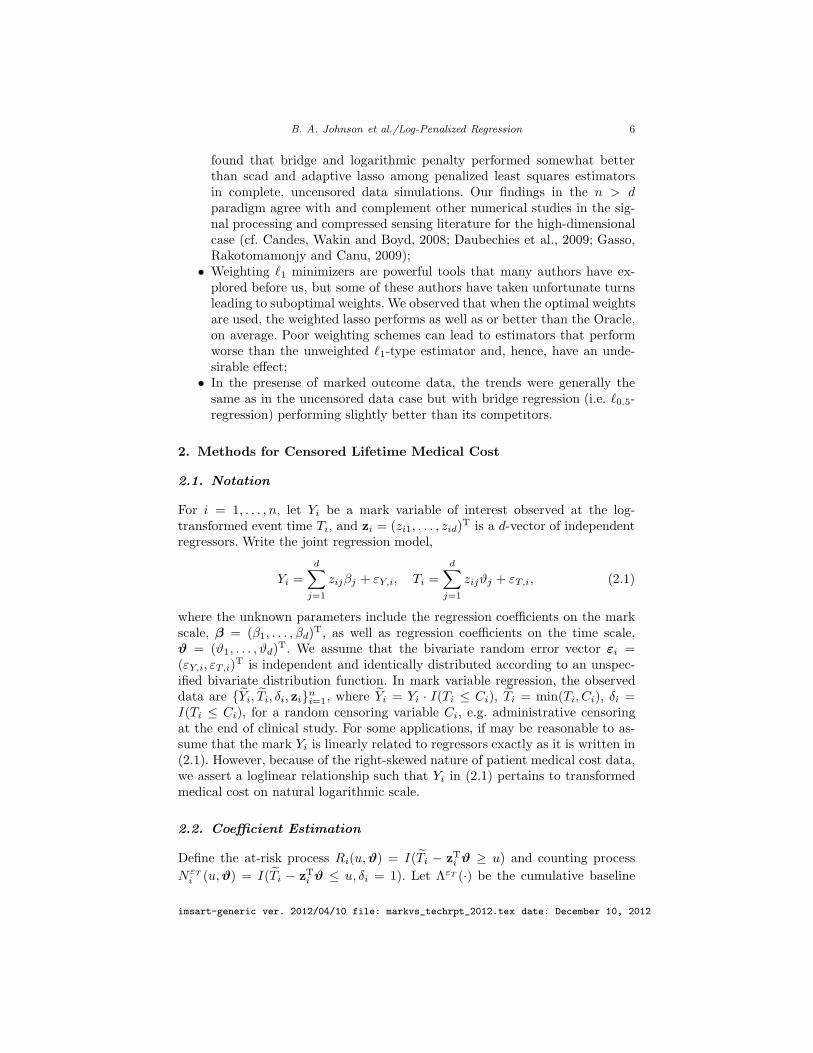
This paper is concerned with data sets where n > d and a natural question iswhether log penalized least squares regression can apply to high-dimensionaldata also. To illustrate fitting high-dimensional data via Algorithm 1, we sim-ulated one data set with n = 40 and d = 60. Six coefficients were non-zeroand the design matrix was standard normal with identity covariance matrix.We plot the coefficient paths for four estimators — lasso, logarithmic penalty,bridge (ℓ0.5), and optimal adaptive lasso — all using coordinate-wise optimiza-tion. The optimal adaptive lasso uses weights wj = 1/(|β0j + ǫ). The coefficientpaths are displayed in Figure 3. We note that lasso and optimal adaptive lasso(AL(Opt)) have smoother coefficient paths than either bridge and logarithmicpenalty because they are exact solutions to convex optimization problems. How-ever, as far as we can tell, the smoothness of the coefficient path has modestvalue in practical work.

There is no conceptual difficulty in extending Algorithm 1 to computingcoefficient paths on the mark-scale for censored medical cost data after an initialestimate ϑ∗ on the time-scale is computed. But choosing the best coefficientestimate on the time-scale that leads to optimal model performance on themark-scale is challenging. A second challenge is to conceive of a new strategyfor parameter tuning that does not rely on an estimate of the coefficients fromthe full model. We have no direct evidence to suggest a concrete solution toeither of these challenges. Johnson, Long and Chung (2011) considered a relatedproblem in unbiased transformations for censored outcomes in high-dimensionaldata where they first screen the data, estimate coefficients on the smaller subset,then impute the censored outcomes. A similar heuristic could be applied toour problem here on the time-scacle, then use these estimates to calibrate thecoefficient estimates on the mark-scale. As we have no data to motivate theseinvestigations, we leave these problems for future work.



−6 −4 −2 0−4

−2

0

2

4

log(λ)

AL(Opt)

−6 −4 −2 0−4

−2

0

2

4

log(λ)

Log

−6 −4 −2 0−4

−2

0

2

4

log(λ)

Lasso

−6 −4 −2 0−4

−2

0

2

4

log(λ)

Bridge

Fig 3. Regularized coefficient paths for data set with n < d.



7. Discussion

In this paper, we reviewed, adopted, and extended iteratively reweighted ℓ1 min-imization to achieve simultaneous coefficient estimation and variable selectionin regression models. The basic asymptotic theory behind log-penalized leastsquares estimators was presented elsewhere Zou and Li (2008); Johnson, Linand Zeng (2008) but inferior computational algorithms were presented in thosepapers. We present a better numerical algorithm using ideas from the signalprocessing literature Candes, Wakin and Boyd (2008). In our limited simula-tion studies for uncensored data, the log-penalized least squares estimator hadsomewhat better operating characteristics than adaptive lasso and scad. Whileone numerical study is not enough evidence to draw any final conclusions, ourfindings generally agree with those reported elsewhere (Gasso, Rakotomamonjyand Canu, 2009) albeit in a different setup.

We presented a new family of ℓ1-regularized variable selection procedures forcensored medical cost through an extension of Huang’s (2002) calibration esti-mator. The problem is more challenging than variable selection in survival databecause of the induced dependent censorship and joint modeling. By carefullychoosing weight functions, we can write the solution to the penalized estimatingequations into the minimizer of a penalized least squares objective function, witha surrogate least squares loss function. This simplification leads to a substantialimprovement in the constrained, convex optimization and allows us to performsimultaneous coefficient estimation and variable selection through optimizationtransfer. We propose information-based model selection criteria for our prob-lem through a new dispersion statistic. The asymptotic theory says that thelog-penalized calibration estimator for lifetime medical cost possesses an oracleproperty. Simulation studies confirms that our log-penalized estimator performswell in practice.

Appendix A: Large Sample Theory

In this section we outline the oracle property for the proposed log-penalizedestimator of lifetime medical cost. This theory makes use of existing asymptotictheories for Huang’s (2002) calibration estimator and a theory of penalizedestimating functions by Johnson, Lin and Zeng (2008). To begin, we review theasymptotic properties of Huang’s (2002) estimator.

Define θ = (βT,ϑT)T and the “stacked” estimating function, Sε(θ) = STεY (θ), STεT (ϑ)T.Define θFull as the zero-crossing of the estimating equations, 0 = Sε(θ). Under

Conditions A-E in Huang (2002, Appendix), θFull is strongly consistent for the

true coefficient vector θ0 and n1/2(θFull−θ0) converges in distribution to a mean-

zero normal random vector with covariance V = Λ−1ΩΛ−1, where Λ ≡ Λ(θ0)is the asymptotic slope matrix of Sε(θ) evaluated at θ = θ0 (see Huang, 2002,expression (A.2) in the Appendix) and Ω ≡ Ω(θ0) is the asymptotic covarianceof n−1/2

Sε(θ0).



To state the oracle property, we need some additional notation. Define thetrue active set A = j|β0j 6= 0, j = 1, . . . , d, its complement set Ac = j|β0j =0, j = 1, . . . , d, as well as the sample quantities An = j|βj 6= 0, j = 1, . . . , dand similarly for Ac

n. Define the stacked penalized estimating function,

SPε (θ) =

(SεY (θ)SεT (ϑ)

)−(nλns(β)|β|−1

0

),

and the partitioned asymptotic covariance V:

V =

(VY Y VY T

VTY VTT

)=

VYAYAVYAYAc VYAT

VYAcYAVYAcYAc VYAcT

VTYAVTYAc VTT

.

If the true active set were known a priori, then the asymptotic covariance of theoracle estimator would be

VO =

(VYAYA

VYAT

VTYAVTT

)= Λ−1

O ΩOΛ−1O ,

Theorem A.1. Under Conditions A-E in Huang (2002, Appendix), n−1/2λn →0 and λn → ∞, the following results hold:

(i) Sparsity: limn→∞ P (An = A) = 1;(ii) Asymptotic normality:

n1/2(ΛO + Γ)θA − θA + (ΛO + Γ)−1bn

→d N(0,ΩO),

where Γ = diag(0d, λns(βA)β−2A ) and bn = (0T

d , (λns(βA)|βA|−1)T)T.

The proof of Theorem A.1 follows as a direct consequence of Johnson, Linand Zeng (2008) and is omitted. For general weight funcitonsWεY (t, θ) in Sε(θ),Huang’s estimator results in an approximate zero-crossing due to potential mul-tiple zero-crossings of the original unregularized esimating function Sε(θ). How-ever, by restricting the class of weight functions WεY (t, θ) to depend on ϑ only(i.e. not on β) and choosing the specific marked process with ψ(t) = t, thesolution to the penalized estimating function S

Pε (θ) is exact (Johnson, Lin and

Zeng, 2008).

References

Andersen, P. K., Borgan, O., Gill, R. D. and Keiding, N. (1993). Sta-tistical models based on counting processes. Springer, New York.

Bang, H. and Tsiatis, A. A. (2000). Estimating medical costs with censoreddata. Biometrika 87 329–343.

Buhlmann, P. and Meier, L. (2008). Discussion: One-step sparse estimatesin nonconcave penalized likelihood models. Ann. Statist. 36 1534-1541.



Candes, E. J., Wakin, M. B. and Boyd, S. (2008). Enhancing Sparsity byReweighted ℓ1-minimization. J. Fourier Analysis and Applications 14 877-905.

Daubechies, I., DeVore, R., Fornasier, M. and Sinan Gunturk, S.

(2009). Iteratively reweighted least squares minimization for sparse recovery.Comm. Pure and Appl. Math. 2009 1-38.

Efron, B., Hastie, T., Johnstone, I. and Tibshirani, R. (2004). LeastAngle Regression. Annals of Statistics 32 407-451.

Fan, J. and Li, R. (2001). Variable Selection via Nonconcave Penalized Like-lihood and its Oracle Properties. Journal of the American Statistical Associ-ation 96 1348-1360.

Frank, I. E. and Friedman, J. H. (1993). A statistical view of some chemo-metrics regression tools. Technometrics 35 109-148.

Friedman, J.,Hastie, T.,Hofling, H. andTibshirani, R. (2007). Pathwisecoordinate optimization. The Annals of Applied Statistics 1 302–332.

Fu, W. (2003). Penalized Estimating Equations. Biometrics 59 126-132.Gasso, G., Rakotomamonjy, A. and Canu, S. (2009). Recovering sparsesignals with a certain famiily of nonconvex penalties and DC programming.IEEE Trans. Signal Processing 57 4686-4698.

Huang, Y. (2002). Calibration Regression of Censored Lifetime Medical Cost.Journal of the American Statistical Association 97 318-327.

Huang, Y. and Louis, T. A. (1998). Nonparametric estimation of the jointdistribution of survival time and mark variables. Biometrika 85 785–798.

Huang, Y. and Lovato, L. (2002). Tests for lifetime utility or cost via cali-brating survial time. Statistica Sinica 12 707–723.

Huang, J., Ma, S. and Zhang, C. H. (2008). Adaptive lasso for sparse high-dimensional regression models. Statistica Sinica 18 1603-1618.

Hunter, D. R. and Li, R. (2005). Variable selection using MM algorithms.Ann. Statist. 33 1617–1642.

Jain, A. K. and Strawderman, R. L. (2002). Flexible hazard regressionmodeling for medical cost data. Biostatistics 3 101-118.

Johnson, B. A., Lin, D. Y. and Zeng, D. (2008). Penalized estimating func-tions and variable seleciton in semiparametric regression models. Journal ofthe American Statistical Association 103 672–680.

Johnson, B. A., Long, Q. and Chung, M. (2011). On path restoration forcensored outcomes. Biometrics 67 1379-1388.

Kalbfleisch, J. D. and Prentice, R. L. (2002). The statistical analysis offailure time data, 2 ed. Wiley New York.

Kelly, K., Crowley, J., Bunn Jr., P. A., Presant, C. A., Grevs-

tad, P. K., Moinpour, C. M., Ramsey, S. D., Wozniak, A. J.,Weiss, G. R., Moore, D. R., Israel, V. K., Livingston, R. B. andGandra, D. R. (2001). Randomized Phase III Trial of Paclitaxel Plus Car-boplatin Versus Vinorelbine Plus Cisplatin in the Treatment of Patients withAdvanced Non-Small Cell Lung Cancer: A Southwest Oncology Group Trial.Journal of Clinical Oncology 19 3210–3218.

Lin, D. Y., Feuer, R. E. J. amd Etzioni and Wax, Y. (1997). Estimating



medical costs from incomplete follow-up. Biometrics 53 419–434.Meinshausen, N. and Buhlmann, P. (2006). Variable Selection and High-Dimensional Graphs With the Lasso. Annals of Statistics 34 1436-1462.

Osborne, M., Presnell, B. and Turlach, B. (2000). On the lasso and itsdual. Journal of Computational and Graphical Statistics 9 389-403.

Tibshirani, R. (1996). Regression shrinkage and selection via the lasso. Journalof the Royal Statistical Society. Series B (Methodological) 58(1) 267–288.

Tsiatis, A. A. (1990). Estimating regression parameters using linear rank testsfor censored data. The Annals of Statistics 18(1) 354–372.

Wei, L. J., Ying, Z. and Lin, D. Y. (1990). Linear regression analysis ofcensored survival data based on rank tests. Biometrika 77 845-851.

Zhao, P. and Yu, B. (2006). On Model Selection Consistency of Lasso. Journalof Machine Learning Research 7 2541-2563.

Zou, H. (2006). The adaptive lasso and its oracle properties. Journal of theAmerican Statistical Association 101 1418–1429.

Zou, H. and Li, R. (2008). One-step sparse estimates in nonconcave penalizedlikelihood models. Annals of Statistics 36 1509-1533.



Table 1

Coefficient estimates for SWOG 9509 data from the full model, lasso, and logarithmicpenalty. Table entries are multiplied by 100.

Full Lasso LogVar. AIC BIC AIC BIC

Gehan weight1. trt 16.74 13.56 9.44 15.37 9.992. sex 15.33 5.49 1.96 8.09 3.623. progstat 35.75 30.55 26.25 32.68 31.354. ps -10.34 -8.51 -6.48 -8.12 -3.295. stage 8.11 0.56 0 2.07 06. pleural 3.31 0 0 0 07. weight 5.32 1.70 0 0.73 08. height -11.64 0 0 0 09. creat 4.75 1.35 0 0.29 010. albumin 13.65 8.52 2.79 11.12 3.3511. calcium -10.36 -5.38 0 -7.81 012. ldh -4.21 0 0 0 013. alkptase -3.74 0 0 0 014. bilirubin 8.31 3.41 0 3.72 015. wbc -15.24 -11.66 -8.22 -14.17 -10.3416. platelet -2.80 -2.59 0 0 017. hgb 6.70 5.55 4.87 4.94 018. age -1.14 0 0 0 0

Logrank weight1. trt 12.56 7.43 3.65 7.56 0.132. sex -0.72 0 0 0 03. progstat 35.00 26.95 22.66 31.57 28.874. ps -19.89 -14.23 -10.95 -15.07 -11.765. stage -5.60 -4.58 0 0 06. pleural 12.84 2.03 0 4.63 07. weight 2.75 0 0 0 08. height -13.29 0 0 -0.35 09. creat 15.78 1.69 0 4.57 010. albumin 16.90 9.31 3.70 10.83 3.3111. calcium -16.22 -6.24 0 -8.23 012. ldh -17.89 -9.49 -4.23 -9.21 -2.2113. alkptase -6.86 0 0 0 014. bilirubin 12.67 4.38 0 5.06 015. wbc -17.83 -12.46 -8.74 -12.69 -8.1016. platelet 0.38 -0.91 0 0 017. hgb 15.05 11.86 9.80 11.64 6.6018. age -5.44 0 0 0 0



Table 2

Simulation results comparing regularizations for uncensored data in a least squaresframework. Table entries include median ℓ2 error, median model error (ME), average

number of false positives (FP) and average number of false negatives (FN).

σ2 = 2 σ2 = 9

Method ‖β − β0‖2 ME FP FN ‖β − β0‖2 ME FP FN

ρ = 0.25Full 2.02 1.80 22.00 0 8.76 7.84 22.00 0Lasso 1.32 1.25 9.33 0 5.06 5.13 8.39 0.43Scad 0.81 0.72 3.33 0 6.39 5.74 6.30 0.94Hard 1.63 1.40 8.03 0 7.27 6.57 4.78 1.29MSAL 1.32 1.20 2.48 0 6.68 5.93 3.52 1.40Bridge 0.88 0.79 2.10 0 5.45 4.99 2.44 1.70Log 0.74 0.70 1.35 0.01 6.25 5.67 2.14 2.15AL(Z) 0.88 0.82 2.88 0 5.64 5.45 4.42 1.25AL(H) 2.08 1.88 11.54 0.20 7.81 7.37 6.61 1.51AL(Opt) 0.54 0.51 0.11 0 2.38 2.23 0.08 0Oracle 0.85 0.80 0 0 2.65 2.53 0 0

ρ = 0.75Full 5.97 1.70 22.00 0 28.44 8.14 22.00 0Lasso 2.58 0.97 9.25 0.03 10.89 4.61 8.69 1.21Scad 3.60 1.13 3.15 0.87 25.76 7.52 4.55 4.96Hard 5.27 1.55 10.25 0.23 28.39 8.07 10.51 2.86MSAL 3.61 1.82 2.62 0.60 20.92 7.01 3.42 4.61Bridge 2.64 0.95 1.82 0.53 18.53 6.13 2.19 5.12Log 3.04 0.97 1.48 0.78 19.18 6.22 2.26 4.99AL(Z) 3.17 1.11 3.15 0.55 18.17 6.30 5.14 3.83AL(H) 3.28 1.13 11.53 0.06 13.10 4.76 11.23 1.42AL(Opt) 1.23 0.50 0.04 0 6.48 2.52 0.09 0Oracle 1.51 1.06 0 0 6.60 2.97 0 0



Table 3

Simulation results comparing regularizations for marked outcomes. Table entries includemedian ℓ2 error, median model error (ME), average number of false positives (FP) and

average number of false negatives (FN).

σ2 = 2 σ2 = 9

Method ‖β − β0‖2 ME FP FN ‖β − β0‖2 ME FP FN

ρ = 0.25Full 1.25 1.12 22.00 0 6.32 5.68 22.00 0Lasso 1.01 1.03 10.43 0 4.53 4.5 11.65 0.14Scad 0.59 0.53 2.16 0 4.99 4.45 5.93 0.75Hard 0.65 0.59 1.14 0 5.03 4.37 3.14 1.24MSAL 0.85 0.84 1.72 0 4.78 4.43 4.13 0.88Bridge 0.67 0.63 2.38 0 4.14 3.84 3.89 0.79Log 0.81 0.74 2.17 0 5.45 5.36 5.15 1.57AL(Z) 0.68 0.64 2.18 0 4.33 3.94 5.65 0.53AL(H) 1.10 1.02 11.86 0.07 5.28 4.84 9.25 0.94AL(Opt) 0.48 0.48 0.14 0 2.01 1.94 0.48 0Oracle 0.43 0.41 0 0 1.94 1.86 0 0

ρ = 0.75Full 5.51 1.59 22.00 0 22.45 6.59 22.00 0Lasso 2.86 1.25 9.56 0.08 9.49 4.10 9.01 0.99Scad 4.16 1.47 3.69 0.73 19.83 6.37 5.02 4.06Hard 3.51 1.31 3.12 0.71 20.41 6.37 4.82 4.00MSAL 3.63 1.64 2.89 0.55 16.34 5.71 3.64 3.74Bridge 2.90 1.23 3.18 0.57 13.76 4.76 3.74 3.37Log 4.16 1.56 4.03 1.03 18.38 5.95 4.91 4.23AL(Z) 3.13 1.19 4.68 0.34 14.76 5.08 6.07 2.80AL(H) 4.63 1.68 13.6 0.28 12.73 5.03 12.11 1.41AL(Opt) 1.60 0.71 1.15 0 5.94 2.39 0.78 0.13Oracle 1.16 0.51 0 0 5.43 2.28 0 0


log-penalized least squares, iteratively reweighted lasso, and

Documents