topology of cell complexes - cornell university

Topology of Cell Complexes

Here we collect a number of basic topological facts about CW complexes for con-

venient reference. A few related facts about manifolds are also proved.

Let us first recall from Chapter 0 that a CW complex is a space X constructed in

the following way:

(1) Start with a discrete set X0 , the 0 cells of X .

(2) Inductively, form the n skeleton Xn from Xn−1 by attaching n cells enα via maps

ϕα :Sn−1→Xn−1 . This means that Xn is the quotient space of Xn−1∐αD

nα under

the identifications x ∼ ϕα(x) for x ∈ ∂Dnα . The cell enα is the homeomorphic

image of Dnα − ∂Dnα under the quotient map.

(3) X =⋃nX

n with the weak topology: A set A ⊂ X is open (or closed) iff A∩Xn is

open (or closed) in Xn for each n .

Note that condition (3) is superfluous when X is finite-dimensional, so that X = Xn

for some n . For if A is open in X = Xn , the definition of the quotient topology on

Xn implies that A∩Xn−1 is open in Xn−1 , and then by the same reasoning A∩Xn−2

is open in Xn−2 , and similarly for all the skeleta Xn−i .

Each cell enα has its characteristic map Φα , which is by definition the composi-

tion Dnα Xn−1∐αD

nα→Xn X . This is continuous since it is a composition of

continuous maps, the inclusion Xn X being continuous by (3). The restriction of

Φα to the interior of Dnα is a homeomorphism onto enα .

An alternative way to describe the topology on X is to say that a set A ⊂ X is

open (or closed) iff Φ−1α (A) is open (or closed) in Dnα for each characteristic map Φα .

In one direction this follows from continuity of the Φα ’s, and in the other direction,

suppose Φ−1α (A) is open in Dnα for each Φα , and suppose by induction on n that

A∩Xn−1 is open in Xn−1 . Then since Φ−1α (A) is open in Dnα for all α , A∩Xn is open

in Xn by the definition of the quotient topology on Xn . Hence by (3), A is open in X .

A consequence of this characterization of the topology on X is that X is a quotient

space of∐n,αD

nα .

520 Appendix Topology of Cell Complexes

A subcomplex of a CW complex X is a subspace A ⊂ X which is a union of cells

of X , such that the closure of each cell in A is contained in A . Thus for each cell

in A , the image of its attaching map is contained in A , so A is itself a CW complex.

Its CW complex topology is the same as the topology induced from X , as one sees

by noting inductively that the two topologies agree on An = A ∩ Xn . It is easy to

see by induction over skeleta that a subcomplex is a closed subspace. Conversely, a

subcomplex could be defined as a closed subspace which is a union of cells.

A finite CW complex, that is, one with only finitely many cells, is compact since

attaching a single cell preserves compactness. A sort of converse to this is:

Proposition A.1. A compact subspace of a CW complex is contained in a finite sub-

complex.

Proof: First we show that a compact set C in a CW complex X can meet only finitely

many cells of X . Suppose on the contrary that there is an infinite sequence of points

xi ∈ C all lying in distinct cells. Then the set S = x1, x2, ··· is closed in X . Namely,

assuming S ∩ Xn−1 is closed in Xn−1 by induction on n , then for each cell enα of X ,

ϕ−1α (S) is closed in ∂Dnα , and Φ−1

α (S) consists of at most one more point in Dnα , so

Φ−1α (S) is closed in Dnα . Therefore S∩Xn is closed in Xn for each n , hence S is closed

in X . The same argument shows that any subset of S is closed, so S has the discrete

topology. But it is compact, being a closed subset of the compact set C . Therefore S

must be finite, a contradiction.

Since C is contained in a finite union of cells, it suffices to show that a finite

union of cells is contained in a finite subcomplex of X . A finite union of finite sub-

complexes is again a finite subcomplex, so this reduces to showing that a single cell enαis contained in a finite subcomplex. The image of the attaching map ϕα for enα is com-

pact, hence by induction on dimension this image is contained in a finite subcomplex

A ⊂ Xn−1 . So enα is contained in the finite subcomplex A∪ enα . ⊔⊓

Now we can explain the mysterious letters ‘CW’, which refer to the following two

properties satisfied by CW complexes:

(1) Closure-finiteness: The closure of each cell meets only finitely many other cells.

This follows from the preceding proposition since the closure of a cell is compact,

being the image of a characteristic map.

(2) Weak topology: A set is closed iff it meets the closure of each cell in a closed set.

For if a set meets the closure of each cell in a closed set, it pulls back to a closed

set under each characteristic map, hence is closed by an earlier remark.

In J. H.C.Whitehead’s original definition of CW complexes these two properties played

a more central role. The following proposition contains essentially this definition.

Topology of Cell Complexes Appendix 521

Proposition A.2. Given a Hausdorff space X and a family of maps Φα :Dnα→X ,

then these maps are the characteristic maps of a CW complex structure on X iff :

(i) Each Φα restricts to a homeomorphism from intDnα onto its image, a cell enα ⊂ X ,

and these cells are all disjoint and their union is X .

(ii) For each cell enα , Φα(∂Dnα) is contained in the union of a finite number of cells of

dimension less than n .

(iii) A subset of X is closed iff it meets the closure of each cell of X in a closed set.

Condition (iii) can be restated as saying that a set C ⊂ X is closed iff Φ−1α (C) is

closed in Dnα for all α , since a map from a compact space onto a Hausdorff space is a

quotient map. In particular, if there are only finitely many cells then (iii) is automatic

since in this case the projection∐αD

nα→X is a map from a compact space onto a

Hausdorff space, hence is a quotient map.

For an example where all the conditions except the finiteness hypothesis in (ii)

are satisfied, take X to be D2 with its interior as a 2 cell and each point of ∂D2 as

a 0 cell. The identity map of D2 serves as the Φα for the 2 cell. Condition (iii) is

satisfied since it is a nontrivial condition only for the 2 cell.

Proof: We have already taken care of the ‘only if’ implication. For the converse,

suppose inductively that Xn−1 , the union of all cells of dimension less than n , is a

CW complex with the appropriate Φα ’s as characteristic maps. The induction can start

with X−1= ∅ . Let f :Xn−1

∐αD

nα→Xn be given by the inclusion on Xn−1 and the

maps Φα for all the n cells of X . This is a continuous surjection, and if we can show

it is a quotient map, then Xn will be obtained from Xn−1 by attaching the n cells enα .

Thus if C ⊂ Xn is such that f−1(C) is closed, we need to show that C ∩ emβ is closed

for all cells emβ of X , the bar denoting closure.

There are three cases. If m < n then f−1(C) closed implies C ∩ Xn−1 closed,

hence C ∩emβ is closed since emβ ⊂ Xn−1 . If m = n then emβ is one of the cells enα , so

f−1(C) closed implies f−1(C)∩Dnα is closed, hence compact, hence its image C ∩enαunder f is compact and therefore closed. Finally there is the case m > n . Then

C ⊂ Xn implies C ∩ emβ ⊂ Φβ(∂Dmβ ) . The latter space is contained in a finite union of

e ℓγ ’s with ℓ < m . By induction on m , each C ∩ e ℓγ is closed. Hence the intersection

of C with the union of the finite collection of e ℓγ ’s is closed. Intersecting this closed

set with emβ , we conclude that C ∩ emβ is closed.

It remains only to check that X has the weak topology with respect to the Xn ’s,

that is, a set in X is closed iff it intersects each Xn in a closed set. The preceding

argument with C = Xn shows that Xn is closed, so a closed set intersects each Xn

in a closed set. Conversely, if a set C intersects Xn in a closed set, then C intersects

each enα in a closed set, so C is closed in X by (iii). ⊔⊓


Next we describe a convenient way of constructing open neighborhoods Nε(A) of

subsets A of a CW complex X , where ε is a function assigning a number εα > 0 to each

cell enα of X . The construction is inductive over the skeleta Xn , so suppose we have

already constructed Nnε (A) , a neighborhood of A ∩ Xn in Xn , starting the process

with N0ε (A) = A ∩ X0 . Then we define Nn+1

ε (A) by specifying its preimage under

the characteristic map Φα :Dn+1→X of each cell en+1α , namely, Φ−1

α

(Nn+1ε (A)

)is the

union of two parts: an open εα neighborhood of Φ−1α (A) − ∂D

n+1 in Dn+1− ∂Dn+1 ,

and a product (1− εα,1]×Φ−1α

(Nnε (A)

)with respect to ‘spherical’ coordinates (r , θ)

in Dn+1 , where r ∈ [0,1] is the radial coordinate and θ lies in ∂Dn+1= Sn . Then we

define Nε(A) =⋃nN

nε (A) . This is an open set in X since it pulls back to an open set

under each characteristic map.

Proposition A.3. CW complexes are normal, and in particular, Hausdorff.

Proof: Points are closed in a CW complex X since they pull back to closed sets under

all characteristic maps Φα . For disjoint closed sets A and B in X , we show that Nε(A)

and Nε(B) are disjoint for small enough εα ’s. In the inductive process for building

these open sets, assume Nnε (A) and Nnε (B) have been chosen to be disjoint. For a

characteristic map Φα :Dn+1→X , observe that Φ−1α

(Nnε (A)

)and Φ−1

α (B) are a positive

distance apart, since otherwise by compactness we would have a sequence in Φ−1α (B)

converging to a point of Φ−1α (B) in ∂Dn+1 of distance zero from Φ−1

α

(Nnε (A)

), but

this is impossible since Φ−1α

(Nnε (B)

)is a neighborhood of Φ−1

α (B)∩ ∂Dn+1 in ∂Dn+1

disjoint from Φ−1α

(Nnε (A)

). Similarly, Φ−1

α

(Nnε (B)

)and Φ−1

α (A) are a positive distance

apart. Also, Φ−1α (A) and Φ−1

α (B) are a positive distance apart. So a small enough εαwill make Φ−1

α

(Nn+1ε (A)

)disjoint from Φ−1

α

(Nn+1ε (B)

)in Dn+1 . ⊔⊓

Proposition A.4. Each point in a CW complex has arbitrarily small contractible open

neighborhoods, so CW complexes are locally contractible.

Proof: Given a point x in a CW complex X and a neighborhood U of x in X , we

can choose the εα ’s small enough so that Nε(x) ⊂ U by requiring that the closure of

Nnε (x) be contained in U for each n . It remains to see that Nε(x) is contractible. If

x ∈ Xm−Xm−1 and n > m we can construct a deformation retraction of Nnε (x) onto

Nn−1ε (x) by sliding outward along radial segments in cells enβ , the images under the

characteristic maps Φβ of radial segments in Dn . A deformation retraction of Nε(x)

onto Nmε (x) is then obtained by performing the deformation retraction of Nnε (x)

onto Nn−1ε (x) during the t interval [1/2n,1/2n−1] , points of Nnε (x)−N

n−1ε (x) being

stationary outside this t interval. Finally, Nmε (x) is an open ball about x , and so

deformation retracts onto x . ⊔⊓

In particular, CW complexes are locally path-connected. So a CW complex is path-

connected iff it is connected.


Proposition A.5. For a subcomplex A of a CW complex X , the open neighborhood

Nε(A) deformation retracts onto A if εα < 1 for all α .

Proof: In each cell of X − A , Nε(A) is a product neighborhood of the boundary of

this cell, so a deformation retraction of Nε(A) onto A can be constructed just as in

the previous proof. ⊔⊓

Note that for subcomplexes A and B of X , we have Nε(A)∩Nε(B) = Nε(A∩ B) .

This implies for example that the van Kampen theorem and Mayer-Vietoris sequences

hold for decompositions X = A∪ B into subcomplexes A and B as well as into open

sets A and B .

A map f :X→Y with domain a CW complex is continuous iff its restrictions to

the closures enα of all cells enα are continuous, and it is useful to know that the same

is true for homotopies ft :X→Y . With this objective in mind, let us introduce a

little terminology. A topological space X is said to be generated by a collection of

subspaces Xα if X =⋃αXα and a set A ⊂ X is closed iff A∩ Xα is closed in Xα for

each α . Equivalently, we could say ‘open’ instead of ‘closed’ here, but ‘closed’ is more

convenient for our present purposes. As noted earlier, though not in these words,

a CW complex X is generated by the closures enα of its cells enα . Since every finite

subcomplex of X is a finite union of closures enα , X is also generated by its finite

subcomplexes. It follows that X is also generated by its compact subspaces, or more

briefly, X is compactly generated.

Proposition A.15 later in the Appendix asserts that if X is a compactly generated

Hausdorff space and Z is locally compact, then X×Z , with the product topology, is

compactly generated. In particular, X×I is compactly generated if X is a CW complex.

Since every compact set in X×I is contained in the product of a compact subspace

of X with I , hence in the product of a finite subcomplex of X with I , such product

subspaces also generate X×I . Since such a product subspace is a finite union of

products enα×I , it is also true that X×I is generated by its subspaces enα×I . This

implies that a homotopy F :X×I→Y is continuous iff its restrictions to the subspaces

enα×I are continuous, which is the statement we were seeking.

Products of CW Complexes

There are some unexpected point-set-topological subtleties that arise with prod-

ucts of CW complexes. As we shall show, the product of two CW complexes does have

a natural CW structure, but its topology is in general finer, with more open sets, than

the product topology. However, the distinctions between the two topologies are rather

small, and indeed nonexistent in most cases of interest, so there is no real problem

for algebraic topology.

Given a space X and a collection of subspaces Xα whose union is X , these sub-

spaces generate a possibly finer topology on X by defining a set A ⊂ X to be open


iff A ∩ Xα is open in Xα for all α . The axioms for a topology are easily verified for

this definition. In case Xα is the collection of compact subsets of X , we write Xcfor this new compactly generated topology. It is easy to see that X and Xc have the

same compact subsets, and the two induced topologies on these compact subsets co-

incide. If X is compact, or even locally compact, then X = Xc , that is, X is compactly

generated.

Theorem A.6. For CW complexes X and Y with characteristic maps Φα and Ψβ ,

the product maps Φα×Ψβ are the characteristic maps for a CW complex structure

on (X×Y)c . If either X or Y is compact or more generally locally compact, then

(X×Y)c = X×Y . Also, (X×Y)c = X×Y if both X and Y have countably many

cells.

Proof: For the first statement it suffices to check that the three conditions in Propo-

sition A.2 are satisfied when we take the space ‘X ’ there to be (X×Y)c . The first two

conditions are obvious. For the third, which says that (X×Y)c is generated by the

products emα ×enβ , observe that every compact set in X×Y is contained in the prod-

uct of its projections onto X and Y , and these projections are compact and hence

contained in finite subcomplexes of X and Y , so the original compact set is contained

in a finite union of products emα ×enβ . Hence the products emα ×e

nβ generate (X×Y)c .

The second assertion of the theorem is a special case of Proposition A.15, hav-

ing nothing to do with CW complexes, which says that a product X×Y is compactly

generated if X is compactly generated Hausdorff and Y is locally compact.

For the last statement of the theorem, suppose X and Y each have at most count-

ably many cells. For an open set W ⊂ (X×Y)c and a point (a, b) ∈ W we need to find

a product U×V ⊂ W with U an open neighborhood of a in X and V an open neigh-

borhood of b in Y . Choose finite subcomplexes X1 ⊂ X2 ⊂ ··· of X with X =⋃iXi ,

and similarly for Y . We may assume a ∈ X1 and b ∈ Y1 . Since the two topologies

agree on X1×Y1 , there is a compact product neighborhood K1×L1 ⊂ W of (a, b)

in X1×Y1 . Assuming inductively that Ki×Li ⊂ W has been constructed in Xi×Yi ,

we would like to construct Ki+1×Li+1 ⊂ W as a compact neighborhood of Ki×Li in

Xi+1×Yi+1 . To do this, we first choose for each x ∈ Ki compact neighborhoods Kxof x in Xi+1 and Lx of Li in Yi+1 such that Kx×Lx ⊂ W , using the compactness

of Li . By compactness of Ki , a finite number of the Kx ’s cover Ki . Let Ki+1 be the

union of these Kx ’s and let Li+1 be the intersection of the corresponding Lx ’s. This

defines the desired Ki+1×Li+1 . Let Ui be the interior of Ki in Xi , so Ui ⊂ Ui+1 for

each i . The union U =⋃iUi is then open in X since it intersects each Xi in a union

of open sets and the Xi ’s generate X . In the same way the Li ’s yield an open set V

in Y . Thus we have a product of open sets U×V ⊂ W containing (a, b) . ⊔⊓

We will describe now an example from [Dowker 1952] where the product topology

on X×Y differs from the CW topology. Both X and Y will be graphs consisting of


infinitely many edges emanating from a single vertex, with uncountably many edges

for X and countably many for Y .

Let X =∨s Is where Is is a copy of the interval [0,1] and the index s ranges

over all infinite sequences s = (s1, s2, ···) of positive integers. The wedge sum is

formed at the 0 endpoint of Is . Similarly we let Y =∨j Ij but with j varying just

over positive integers. Let psj be the point (1/sj ,1/sj) ∈ Is×Ij ⊂ X×Y and let P be

the union of all these points psj . Thus P consists of a single point in each 2 cell of

X×Y , so P is closed in the CW topology on X×Y . We will show it is not closed in the

product topology by showing that (x0, y0) lies in its closure, where x0 is the common

endpoint of the intervals Is and y0 is the common endpoint of the intervals Ij .

A basic open set containing (x0, y0) in the product topology has the form U×V

where U =∨s [0, as) and V =

∨j [0, bj) . It suffices to show that P has nonempty

intersection with U×V . Choose a sequence t = (t1, t2, ···) with tj > j and tj > 1/bjfor all j , and choose an integer k > 1/at . Then tk > k > 1/at hence 1/tk < at . We

also have 1/tk < bk . So (1/tk,1/tk) is a point of P that lies in [0, at)×[0, bk) and

hence in U×V .

Euclidean Neighborhood Retracts

At certain places in this book it is desirable to know that a given compact space

is a retract of a finite simplicial complex, or equivalently (as we shall see) a retract of

a neighborhood in some Euclidean space. For example, this condition occurs in the

Lefschetz fixed point theorem, and it was used in the proof of Alexander duality. So

let us study this situation in more detail.

Theorem A.7. A compact subspace K of Rn is a retract of some neighborhood iff K

is locally contractible in the weak sense that for each x ∈ K and each neighborhood

U of x in K there exists a neighborhood V ⊂ U of x such that the inclusion VU

is nullhomotopic.

Note that if K is a retract of some neighborhood, then it is a retract of every

smaller neighborhood, just by restriction of the retraction. So it does not matter if we

require the neighborhoods to be open. Similarly it does not matter if the neighbor-

hoods U and V in the statement of the theorem are required to be open.

Proof: Let us do the harder half first, constructing a retraction of a neighborhood

of K onto K under the local contractibility assumption. The first step is to put a

CW structure on the open set X = Rn− K , with the size of the cells approaching

zero near K . Consider the subdivision of Rn into unit cubes of dimension n with

vertices at the points with integer coordinates. Call this collection of cubes C0 . For

an integer k > 0, we can subdivide the cubes of C0 by taking n dimensional cubes of

edgelength 1/2k with vertices having coordinates of the form i/2k for i ∈ Z . Denote

this collection of cubes by Ck . Let A0 ⊂ C0 be the set of cubes disjoint from K , and


inductively, let Ak ⊂ Ck be the set of cubes disjoint from K and not contained in cubes

of Aj for j < k . The open set X is then the union of all the cubes in the combined

collection A =⋃kAk . Note that the collection A is locally finite: Each point of X has

a neighborhood meeting only finitely many cubes in A , since the point has a positive

distance from the closed set K .

If two cubes of A intersect, their intersection is an i dimensional face of one

of them for some i < n . Likewise, when two faces of cubes of A intersect, their

intersection is a face of one of them. This implies that the open faces of cubes of A

that are minimal with respect to inclusion among such faces form the cells of a CW

structure on X , since the boundary of such a face is a union of such faces. The vertices

of this CW structure are thus the vertices of all the cubes of A , and the n cells are

the interiors of the cubes of A .

Next we define inductively a subcomplex Z of this CW structure on X and a map

r :Z→K . The 0 cells of Z are exactly the 0 cells of X , and we let r send each 0 cell

to the closest point of K , or if this is not unique, any one of the closest points of

K . Assume inductively that Zk and r :Zk→K have been defined. For a cell ek+1 of

X with boundary in Zk , if the restriction of r to this boundary extends over ek+1

then we include ek+1 in Zk+1 and we let r on ek+1 be such an extension that is not

too large, say an extension for which the diameter of its image r(ek+1) is less than

twice the infimum of the diameters for all possible extensions. This defines Zk+1 and

r :Zk+1→K . At the end of the induction we set Z = Zn .

It remains to verify that by letting r equal the identity on K we obtain a contin-

uous retraction Z ∪ K→K , and that Z ∪ K contains a neighborhood of K . Given a

point x ∈ K , let U be a ball in the metric space K centered at x . Since K is locally

contractible, we can choose a finite sequence of balls in K centered at x , of the form

U = Un ⊃ Vn ⊃ Un−1 ⊃ Vn−1 ⊃ ··· ⊃ U0 ⊃ V0 , each ball having radius equal to some

small fraction of the radius of the preceding one, and with Vi contractible in Ui . Let

B ⊂ Rn be a ball centered at x with radius less than half the radius of V0 , and let Y

be the subcomplex of X formed by the cells whose closures are contained in B . Thus

Y ∪ K contains a neighborhood of x in Rn . By the choice of B and the definition

of r on 0 cells we have r(Y 0) ⊂ V0 . Since V0 is contractible in U0 , r is defined

on the 1 cells of Y . Also, r(Y 1) ⊂ V1 by the definition of r on 1 cells and the fact

that U0 is much smaller than V1 . Similarly, by induction we have r defined on Y i

with r(Y i) ⊂ Vi for all i . In particular, r maps Y to U . Since U could be arbitrarily

small, this shows that extending r by the identity map on K gives a continuous map

r :Z ∪ K→K . And since Y ⊂ Z , we see that Z ∪ K contains a neighborhood of K by

the earlier observation that Y ∪K contains a neighborhood of x . Thus r :Z ∪K→K

retracts a neighborhood of K onto K .

Now for the converse. Since open sets in Rn are locally contractible, it suffices to

show that a retract of a locally contractible space is locally contractible. Let r :X→A


be a retraction and let U ⊂ A be a neighborhood of a given point x ∈ A . If X is

locally contractible, then inside the open set r−1(U) there is a neighborhood V of

x that is contractible in r−1(U) , say by a homotopy ft :V→r−1(U) . Then V ∩ A is

contractible in U via the restriction of the composition rft . ⊔⊓

A space X is called a Euclidean neighborhood retract or ENR if for some n there

exists an embedding i :XRn such that i(X) is a retract of some neighborhood in

Rn . The preceding theorem implies that the existence of the retraction is independent

of the choice of embedding, at least when X is compact.

Corollary A.8. A compact space is an ENR iff it can be embedded as a retract of a

finite simplicial complex. Hence the homology groups and the fundamental group of

a compact ENR are finitely generated.

Proof: A finite simplicial complex K with n vertices is a subcomplex of a simplex

∆n−1 , and hence embeds in Rn . The preceding theorem then implies that K is a

retract of some neighborhood in Rn , so any retract of K is also a retract of such a

neighborhood, via the composition of the two retractions. Conversely, let K be a com-

pact space that is a retract of some open neighborhood U in Rn . Since K is compact

it is bounded, lying in some large simplex ∆n ⊂ Rn . Subdivide ∆n , say by repeated

barycentric subdivision, so that all simplices of the subdivision have diameter less

than the distance from K to the complement of U . Then the union of all the sim-

plices in this subdivision that intersect K is a finite simplicial complex that retracts

onto K via the restriction of the retraction U→K . ⊔⊓

Corollary A.9. Every compact manifold, with or without boundary, is an ENR.

Proof: Manifolds are locally contractible, so it suffices to show that a compact man-

ifold M can be embedded in Rk for some k . If M is not closed, it embeds in the

closed manifold obtained from two copies of M by identifying their boundaries. So

it suffices to consider the case that M is closed. By compactness there exist finitely

many closed balls Bni ⊂ M whose interiors cover M , where n is the dimension of

M . Let fi :M→Sn be the quotient map collapsing the complement of the interior

of Bni to a point. These fi ’s are the components of a map f :M→(Sn)m which is

injective since if x and y are distinct points of M with x in the interior of Bni , say,

then fi(x) ≠ fi(y) . Composing f with an embedding (Sn)mRk , for example the

product of the standard embeddings Sn Rn+1 , we obtain a continuous injection

MRk , and this is a homeomorphism onto its image since M is compact. ⊔⊓

Corollary A.10. Every finite CW complex is an ENR.

Proof: Since CW complexes are locally contractible, it suffices to show that a finite CW

complex can be embedded in some Rn . This is proved by induction on the number


of cells. Suppose the CW complex X is obtained from a subcomplex A by attaching

a cell ek via a map f :Sk−1→A , and suppose that we have an embedding A Rm .

Then we can embed X in Rk×R

m×R as the union of Dk×0×0 , 0×A×1 ,

and all line segments joining points (x,0,0) and (0, f (x),1) for x ∈ Sk−1 . ⊔⊓

Spaces Dominated by CW Complexes

We have been considering spaces which are retracts of finite simplicial complexes,

and now we show that such spaces have the homotopy type of CW complexes. In fact,

we can just as easily prove something a little more general than this. A space Y is

said to be dominated by a space X if there are maps Yi-----→ X

r-----→ Y with ri ≃ 11.

This makes the notion of a retract into something that depends only on the homotopy

types of the spaces involved.

Proposition A.11. A space dominated by a CW complex is homotopy equivalent to a

CW complex.

Proof: Recall from §3.F that the mapping telescopeT(f1, f2, ···) of a sequence of

maps X1

f1------------→X2

f2------------→X3 ------------→ ··· is the quotient space of

∐i

(Xi×[i, i+1]

)obtained

by identifying (x, i + 1) ∈ Xi×[i, i + 1] with (f (x), i + 1) ∈ Xi+1×[i + 1, i + 2] . We

shall need the following elementary facts:

(1) T(f1, f2, ···) ≃ T(g1, g2, ···) if fi ≃ gi for each i .

(2) T(f1, f2, ···) ≃ T(f2, f3, ···) .

(3) T(f1, f2, ···) ≃ T(f2f1, f4f3, ···) .

The second of these is obvious. To prove the other two we will use Proposition 0.18,

whose proof applies not just to CW pairs but to any pair (X1, A) for which there

is a deformation retraction of X1×I onto X1×0 ∪ A×I . To prove (1) we regard

T(f1, f2, ···) as being obtained from∐i

(Xi×i

)by attaching

∐i

(Xi×[i, i + 1]

).

Then we can obtain T(g1, g2, ···) by varying the attaching map by homotopy. To

prove (3) we view T(f1, f2, ···) as obtained from the disjoint union of the mapping

cylinders M(f2i) by attaching∐i

(X2i−1×[2i − 1,2i]

). By sliding the attachment of

X2i−1×[2i − 1,2i] to X2i ⊂ M(f2i) down the latter mapping cylinder to X2i+1 we

convert M(f2i−1) ∪M(f2i) into M(f2if2i−1) ∪M(f2i) . This last space deformation

retracts onto M(f2if2i−1) . Doing this for all i gives the homotopy equivalence in (3).

Now to prove the proposition, suppose that the space Y is dominated by the CW

complex X via maps Yi-----→X

r-----→Y with ri ≃ 11. By (2) and (3) we have T(ir , ir , ···) ≃

T(r , i, r , i, ···) ≃ T(i, r , i, r , ···) ≃ T(ri, r i, ···) . Since ri ≃ 11, T(ri, r i, ···) is ho-

motopy equivalent to the telescope of the identity maps Y→Y→Y→ ··· , which

is Y×[0,∞) ≃ Y . On the other hand, the map ir is homotopic to a cellular map

f :X→X , so T(ir , ir , ···) ≃ T(f , f , ···) , which is a CW complex. ⊔⊓

The Compact-Open Topology Appendix 529

One might ask whether a space dominated by a finite CW complex is homotopy

equivalent to a finite CW complex. In the simply-connected case this follows from

Proposition 4C.1 since such a space has finitely generated homology groups. But

there are counterexamples in the general case; see [Wall 1965].

In view of Corollary A.10 the preceding proposition implies:

Corollary A.12. A compact manifold is homotopy equivalent to a CW complex. ⊔⊓

One could ask more refined questions. For example, do all compact manifolds

have CW complex structures, or even simplicial complex structures? Answers here

are considerably harder to come by. Restricting attention to closed manifolds for

simplicity, the present status of these questions is the following. For manifolds of

dimensions less than 4, simplicial complex structures always exist. In dimension 4

there are closed manifolds that do not have simplicial complex structures, while the

existence of CW structures is an open question. In dimensions greater than 4, CW

structures always exist, but whether simplicial structures always exist is unknown,

though it is known that there are n manifolds not having simplicial structures locally

isomorphic to any linear simplicial subdivision of Rn , for all n ≥ 4. For more on

these questions, see [Kirby & Siebenmann 1977] and [Freedman & Quinn 1990].

Exercises

1. Show that a covering space of a CW complex is also a CW complex, with cells

projecting homeomorphically onto cells.

2. Let X be a CW complex and x0 any point of X . Construct a new CW complex

structure on X having x0 as a 0 cell, and having each of the original cells a union of

the new cells. The latter condition is expressed by saying the new CW structure is a

subdivision of the old one.

3. Show that a CW complex is path-connected iff its 1 skeleton is path-connected.

4. Show that a CW complex is locally compact iff each point has a neighborhood that

meets only finitely many cells.

5. For a space X , show that the identity map Xc→X induces an isomorphism on π1 ,

where Xc denotes X with the compactly generated topology.

The Compact-Open Topology

By definition, the compact-open topology on the space XY of maps f :Y→X has

a subbasis consisting of the sets M(K,U) of mappings taking a compact set K ⊂ Y

to an open set U ⊂ X . Thus a basis for XY consists of sets of maps taking a finite

number of compact sets Ki ⊂ Y to open sets Ui ⊂ X . If Y is compact, which is the

only case we consider in this book, convergence to f ∈ XY means, loosely speaking,

that finer and finer compact covers Ki of Y are taken to smaller and smaller open

covers Ui of f(Y) . One of the main cases of interest in homotopy theory is when

530 Appendix The Compact-Open Topology

Y = I , so XI is the space of paths in X . In this case one can check that a system of

basic neighborhoods of a path f : I→X consists of the open sets⋂iM(Ki, Ui) where

the Ki ’s are a partition of I into nonoverlapping closed intervals and Ui is an open

neighborhood of f(Ki) .

The compact-open topology is the same as the topology of uniform convergence

in many cases:

Proposition A.13. If X is a metric space and Y is compact, then the compact-open

topology on XY is the same as the metric topology defined by the metric d(f ,g) =

supy∈Y d(f(y), g(y)) .

Proof: First we show that every open ε ball Bε(f ) about f ∈ XY contains a neigh-

borhood of f in the compact-open topology. Since f(Y) is compact, it is covered by

finitely many balls Bε/3(f(yi)

). Let Ki ⊂ Y be the closure of f−1(Bε/3(f (yi))

), so

Ki is compact, Y =⋃i Ki , and f(Ki) ⊂ Bε/2

(f(yi)

)= Ui , hence f ∈

⋂iM(Ki, Ui) .

To show that⋂iM(Ki, Ui) ⊂ Bε(f ) , suppose that g ∈

⋂iM(Ki, Ui) . For any y ∈ Y ,

say y ∈ Ki , we have d(g(y), f (yi)

)< ε/2 since g(Ki) ⊂ Ui . Likewise we have

d(f(y), f (yi)

)< ε/2, so d

(f(y), g(y)

)≤ d

(f(y), f (yi)

)+ d

(g(y), f (yi)

)< ε .

Since y was arbitrary, this shows g ∈ Bε(f ) .

Conversely, we show that for each open set M(K,U) and each f ∈ M(K,U) there

is a ball Bε(f ) ⊂ M(K,U) . Since f(K) is compact, it has a distance ε > 0 from the

complement of U . Then d(f ,g) < ε/2 implies g(K) ⊂ U since g(K) is contained in

an ε/2 neighborhood of f(K) . So Bε/2(f ) ⊂ M(K,U) . ⊔⊓

The next proposition contains some useful properties of the compact-open topol-

ogy from the viewpoint of algebraic topology.

Proposition A.14. (a) The evaluation map e :XY×Y→X , e(f ,y) = f(y) , is con-

tinuous If Y is locally compact.

(b) If f :Y×Z→X is continuous then so is the map f :Z→XY , f (z)(y) = f(y, z) .

(c) The converse to (b) holds when Y is locally compact.

Different definitions of local compactness are common, but the definition we are

using is that Y is locally compact if for each point y ∈ Y and each neighborhood U

of y there is a compact neighborhood V of y contained in U .

In particular, parts (b) and (c) of the proposition provide the point-set topology

justifying the adjoint relation 〈ΣX,Y 〉 = 〈X,ΩY 〉 in §4.3, since they imply that a map

ΣX→Y is continuous iff the associated map X→ΩY is continuous, and similarly for

homotopies of such maps. Namely, think of a basepoint-preserving map ΣX→Y as

a map f : I×X→Y taking ∂I×X ∪ x0×I to the basepoint of Y , so the associated

map f :X→Y I has image in the subspace ΩY ⊂ Y I . A homotopy ft :ΣX→Y gives

a map F : I×X×I→Y taking ∂I×X×I ∪ I×x0×I to the basepoint, with F a map

X×I→ΩY ⊂ Y I defining a basepoint-preserving homotopy ft .

The Compact-Open Topology Appendix 531

Proof: (a) For (f ,y) ∈ XY×Y let U ⊂ X be an open neighborhood of f(y) . Since Y

is locally compact, continuity of f implies there is a compact neighborhood K ⊂ Y

of y such that f(K) ⊂ U . Then M(K,U)×K is a neighborhood of (f ,y) in XY×Y

taken to U by e , so e is continuous at (f ,y) .

(b) Suppose f :Y×Z→X is continuous. To show continuity of f it suffices to show

that for a subbasic set M(K,U) ⊂ XY , the set f−1(M(K,U)) = z ∈ Z | f(K, z) ⊂ U is open in Z . Let z ∈ f−1(M(K,U)) . Since f−1(U) is an open neighborhood of the

compact set K×z , there exist open sets V ⊂ Y and W ⊂ Z whose product V×W

satisfies K×z ⊂ V×W ⊂ f−1(U) . So W is a neighborhood of z in f−1(M(K,U)) .

(c) Note that f :Y×Z→X is the composition Y×Z→Y×XY→X of 11× f and the

evaluation map, so part (a) gives the result. ⊔⊓

We will give three separate applications of Proposition A.14. Here is the first:

Proposition A.15. If X is a compactly generated Hausdorff space and Y is locally

compact, then the product topology on X×Y is compactly generated.

Proof: First a preliminary observation: A function f :X×Y→Z is continuous iff its

restrictions f :C×Y→Z are continuous for all compact C ⊂ X . For, using (b) and (c)

of the preceding Proposition A.14, the first statement is equivalent to f :X→ZY being

continuous and the second statement is equivalent to f :C→ZY being continuous for

all compact C ⊂ X . Then since X is compactly generated, continuity of f :X→ZY is

equivalent to continuity of f :C→ZY for all compact C ⊂ X .

To prove the proposition we just need to show the identity map X×Y→(X×Y)cis continuous. By the previous paragraph, this is equivalent to continuity of the in-

clusion maps C×Y→(X×Y)c for all compact C ⊂ X . Since Y is locally compact, it

is compactly generated, and C is compact Hausdorff hence locally compact, so the

same reasoning shows that continuity of C×Y→(X×Y)c is equivalent to continuity

of C×C′→(X×Y)c for all compact C′ ⊂ Y . But on the compact set C×C′ , the two

topologies on X×Y agree, so we are done. (This proof is from [Dugundji 1966].) ⊔⊓

Returning to the context of Proposition A.14, part (b) of that proposition implies

that there is a well-defined function XY×Z→(XY )Z sending f to f . This is injective,

and part (c) implies that it is surjective if Y is locally compact.

Proposition A.16. The map XY×Z→(XY )Z , f ֏ f , is a homeomorphism if Y is

locally compact Hausdorff and Z is Hausdorff.

Proof: First we show that a subbasis for XY×Z is formed by the sets M(A×B,U)

as A and B range over compact sets in Y and Z respectively and U ranges over

open sets in X . Given a compact K ⊂ Y×Z and a map f ∈ M(K,U) , let KY and

KZ be the projections of K onto Y and Z . Then KY×KZ is compact Hausdorff and

532 Appendix The Compact-Open Topology

hence normal. A normal space has the property that for each closed set C and each

open set O containing C there is another open set O′ containing C whose closure

is contained in O . To see this, apply the normality property to the two closed sets

C and the complement C′ of O , taking O′ to be the resulting open set containing C

and disjoint from an open set containing C′ , so the closure of O′ is contained in O .

Applying this observation to the normal space KY×KZ with C a point k ∈ K and

O = (KY×KZ) ∩ f−1(U) , the result is an open neighborhood of k in KY×KZ whose

closure is contained in f−1(U) . We can take this open neighborhood to be a product

Vk×Wk ⊂ KY×KZ , so its closure is a compact neighborhood Ak×Bk ⊂ f−1(U) of k in

KY×KZ . The sets Vk×Wk for varying k ∈ K form an open cover of the compact set

K so a finite number of the products Ak×Bk cover K . After discarding the others we

then have f ∈⋂kM(Ak×Bk, U) ⊂ M(K,U) , which shows that the sets M(A×B,U)

form a subbasis for XY×Z as claimed.

Under the bijection XY×Z→(XY )Z the sets M(A×B,U) correspond to the sets

M(B,M(A,U)) , so it will suffice to show the latter sets form a subbasis for (XY )Z . We

will show more generally that for any space Q a subbasis for QZ is formed by the sets

M(K,V) as V ranges over a subbasis for Q and K ranges over compact sets in Z ,

assuming that Z is Hausdorff. Then we let Q = XY with subbasis the sets M(A,U) .

Given f ∈ M(K,U) with K compact in Z and U open in Q , write U as a union

of basic sets Uα with each Uα an intersection of finitely many sets Vα,j of the given

subbasis for Q . The cover of K by the open sets f−1(Uα) has a finite subcover,

say by the open sets f−1(Ui) . Since K is compact Hausdorff, hence normal, we can

write K as a union of compact subsets Ki with Ki ⊂ f−1(Ui) , namely, each k ∈ K

has a compact neighborhood Kk contained in some f−1(Ui) with k ∈ f−1(Ui) , so

compactness of K implies that finitely many of these sets Kk cover K and we let Kibe the union of those contained in f−1(Ui) . Now f lies in M(Ki, Ui) = M(Ki,

⋂j Vij) =⋂

jM(Ki, Vij) for each i . Hence f lies in⋂i,jM(Ki, Vij) =

⋂iM(Ki, Ui) ⊂ M(K,U) .

Since⋂i,jM(Ki, Vij) is a finite intersection, this shows that the sets M(K,V) form a

subbasis for QZ . ⊔⊓

Finally, we use Proposition A.14 to prove a very useful fact relating product spaces

and quotient spaces:

Proposition A.17. If f :X→Y is a quotient map then so is f×11 :X×Z→Y×Z

whenever Z is locally compact.

This can be applied when Z = I to show that a homotopy defined on a quotient

space is continuous.

Proof: Consider the diagram at the right, where W is Y×Z

with the quotient topology from X×Z , with g the quotient

map and h the identity. Every open set in Y×Z is open in

W since f×11 is continuous, so it will suffice to show that h is continuous.

The Homotopy Extension Property Appendix 533

Since g is continuous, so is the associated map g :X→WZ , by Proposition A.14.

This implies that h :Y→WZ is continuous since f is a quotient map. Applying Propo-

sition A.14 again, we conclude that h is continuous. ⊔⊓

The Homotopy Extension Property

Near the end of Chapter 0 we stated, and partially proved, an equivalence between

the homotopy extension property and a certain retraction property:

Proposition A.18. A pair (X,A) has the homotopy extension property if and only if

X×0 ∪A×I is a retract of X×I .

Proof: We already gave the easy argument showing that the homotopy extension

property implies the retraction property. The converse was also easy when A is closed

in X , and what we need now is an argument for the converse that does not use this

extra assumption. The argument is from [Strøm 1968].

To simplify the notation, let Y = X×0∪A×I with the subspace topology from

X×I . We will identify X with the subspace X×0 of Y . Assuming there exists a

retraction r :X×I→Y , we will show that a subset O ⊂ Y is open in Y if its intersec-

tions with X and A×I are open in these two subspaces. This implies that a function

on Y is continuous if its restrictions to X and A×I are continuous. Composing such

a function with the retraction then provides the extension to X×I required for the

homotopy extension property.

To show that O is open in Y it suffices to find, for each point x ∈ O , a product

of open sets V×W ⊂ X×I containing x such that (V×W)∩ Y ⊂ O . If x ∈ A×(0,1]

there is no problem doing this, so we may assume x ∈ X . In this case there is also no

problem if x in not in the closure A of A , so we will assume x ∈ A from now on. For

an integer n ≥ 1 let Un be the largest open set in X such that (Un∩A)×[0,1/n) ⊂ O .

The existence of a largest such set Un follows from the fact that a union of open sets

with this property is again an open set with this property. Let U =⋃nUn . Note that

A∩O ⊂ U since O intersects A×I in an open set in A×I by assumption. It will suffice

to show that x ∈ U since if x ∈ Un then we can choose V×W = (Un ∩O)×[0,1/n)

because((Un ∩O)×[0,1/n)

)∩ Y ⊂ O , where Un ∩O is open in X since Un is open

in X .

In order to show that x ∈ U we first consider the point (x, t) for fixed t > 0.

Writing r(x, t) = (r1(x, t), r2(x, t)) ∈ X×I we have r2(x, t) = t since x ∈ A and

r(a, t) = (a, t) for a ∈ A . Thus r(x, t) ∈ A×t so r1(x, t) ∈ A . We claim next that

if r1(x, t) ∈ Un then x ∈ Un . For if r1(x, t) ∈ Un then continuity of r1 implies that

r1(V×(t− ε, t+ ε)) ⊂ Un for some open neighborhood V of x in X and some ε > 0.

In particular r1

((V ∩A)×t

)⊂ Un , or in other words, V ∩A ⊂ Un . By the definition

of Un this implies that V ⊂ Un and hence x ∈ Un since x ∈ V . Thus we have shown

that r1(x, t) ∈ Un implies x ∈ Un .

534 Appendix Simplicial CW Structures

Suppose now that x is not in U . From what we have just shown, this implies that

r1(x, t) ∈ A− U . It follows that r1(x, t) ∈ A−O since A∩O ⊂ U , as noted earlier.

The relation r1(x, t) ∈ A−O holds for arbitrary t > 0, so by letting t approach 0 we

conclude that r1(x,0) ∈ A−O since r1 is a continuous map to X and X ∩O is open

in X . Since r1(x,0) = x we deduce that x is not in O . However, this contradicts the

fact that x was chosen to be a point in O . From this contradiction we conclude that

x must be in U , and the proof is finished. ⊔⊓

For an example of a set O ⊂ X×0 ∪ A×I which is not open even though it

intersects both X×0 and A×I in open sets, let X = [0,1] with A = (0,1] and

O =(x, t) ∈ X×I |||| t < x or t = 0

. Note that in this case there exists no retraction

X×I→X×0∪A×I since the image of a compact set must be compact. This example

also illustrates how the topology on X×0 ∪ A×I as a subspace of X×I can be

different from the topology as the mapping cylinder of the inclusion A X , which

is the quotient topology from X ∐A×I .

Simplicial CW Structures

A D complex can be defined as a CW complex X in which each cell enα is provided

with a distinguished characteristic map σα :∆n→X such that the restriction of σαto each face ∆n−1 of ∆n is the distinguished σβ for some (n − 1) cell en−1

β . It is

understood that the simplices ∆n and ∆n−1 have a specified ordering of their vertices,

and the ordering of the vertices of ∆n induces an ordering of the vertices of each face,

which allows each face to be identified canonically with ∆n−1 . Intuitively, one thinks

of the vertices of each n cell of X as ordered by attaching the labels 0,1, ··· , n near

the vertices, just inside the cell. The vertices themselves do not have to be distinct

points of X .

If we no longer pay attention to orderings of vertices of simplices, we obtain a

weaker structure which could be called an unordered D complex. Here each cell enαhas a distinguished characteristic map σα :∆n→X , but the restriction of σα to a face

of ∆n is allowed to be the composition of σβ :∆n−1→X with a symmetry of ∆n−1

permuting its vertices. Alternatively, we could say that each cell enα has a family of

(n+1)! distinguished characteristic maps ∆n→X differing only by symmetries of ∆n ,

such that the restrictions of these characteristic maps to faces give the distinguished

characteristic maps for (n − 1) cells. The barycentric subdivision of any unordered

∆ complex is an ordered ∆ complex since the vertices of the barycentric subdivision

are the barycenters of the simplices of the original complex, hence have a canonical

ordering according to the dimensions of these simplices. The simplest example of an

unordered ∆ complex that cannot be made into an ordered ∆ complex without sub-

division is ∆2 with its three edges identified by a one-third rotation of ∆2 permuting

the three vertices cyclically.

Simplicial CW Structures Appendix 535

In the literature unordered ∆ complex structures are sometimes called general-

ized triangulations. They can be useful in situations where orderings of vertices are

not needed. One disadvantage of unordered ∆ complexes is that they do not behave

as well with respect to products. The product of two ordered simplices has a canonical

subdivision into ordered simplices using the shuffling operation described in §3.B, and

this allows the product of two ordered ∆ complexes to be given a canonical ordered

∆ complex structure. Without orderings this no longer works.

A CW complex is called regular if its characteristic maps can be chosen to be

embeddings. The closures of the cells are then homeomorphic to closed balls, and so

it makes sense to speak of closed cells in a regular CW complex. The closed cells can

be regarded as cones on their boundary spheres, and these cone structures can be

used to subdivide a regular CW complex into a regular ∆ complex, by induction over

skeleta. In particular, regular CW complexes are homeomorphic to ∆ complexes. The

barycentric subdivision of an unordered ∆ complex is a regular ∆ complex. A sim-

plicial complex is a regular unordered ∆ complex in which each simplex is uniquely

determined by its vertices. In the literature a regular unordered ∆ complex is some-

times called a simplicial multicomplex, or just a multicomplex, to convey the idea that

there can be many simplices with the same set of vertices. The barycentric subdivi-

sion of a regular unordered ∆ complex is a simplicial complex. Hence barycentrically

subdividing an unordered ∆ complex twice produces a simplicial complex.

A major disadvantage of ∆ complexes is that they do not allow quotient con-

structions. The quotient X/A of a ∆ complex X by a subcomplex A is not usually a

∆ complex. More generally, attaching a ∆ complex X to a ∆ complex Y via a simpli-

cial map from a subcomplex A ⊂ X to Y is not usually a ∆ complex. Here a simplicial

map f :A→Y is one that sends each cell enα of A onto a cell ekβ of Y so

that the square at the right commutes, with q a linear surjection send-

ing vertices to vertices, preserving order. To fix this problem we need

to broaden the definition of a ∆ complex to allow cells to be attached

by arbitrary simplicial maps. Thus we define a singular D complex, or s∆ complex,

to be a CW complex with distinguished characteristic maps σα :∆n→X whose re-

strictions to faces are compositions σβq :∆n−1→∆k→X for q a linear surjection

taking vertices to vertices, preserving order. Simplicial maps between s∆ complexes

are defined just as for ∆ complexes. With s∆ complexes one can perform attaching

constructions in the same way as for CW complexes, using simplicial maps instead

of cellular maps to specify the attachments. In particular one can form quotients,

mapping cylinders, and mapping cones. One can also take products by the same

subdivision procedure as for ∆ complexes.

We can view any s∆ complex X as being constructed inductively, skeleton by

skeleton, where the skeleton Xn is obtained from Xn−1 by attaching simplices ∆nvia simplicial maps ∂∆n→Xn−1 that preserve the ordering of vertices in each face


of ∆n . Conversely, any CW complex built in this way is an s∆ complex. For example,

the usual CW structure on Sn consisting of one 0 cell and one n cell is an s∆ complex

structure since the attaching map of the n cell, the constant map, is a simplicial

map from ∂∆n to a point. One can regard this s∆ complex structure as assigning

barycentric coordinates to all points of Sn other than the 0 cell. In fact, an arbitrary

s∆ complex structure can be regarded as just a way of putting barycentric coordinates

in all the open cells, subject to a compatibility condition on how the coordinates

change when one passes from a cell to the cells in its boundary.

Combinatorial Descriptions

The data which specifies a ∆ complex is combinatorial in nature and can be for-

mulated quite naturally in the language of categories. To see how this is done, let

X be a ∆ complex and let Xn be its set of n simplices. The way in which simplices

of X fit together is determined by a ‘face function’ which assigns to each element of

Xn and each (n − 1) dimensional face of ∆n an element of Xn−1 . Thinking of the

n simplex ∆n combinatorially as its set of vertices, which we view as the ordered set

∆n = 0,1, ··· , n , the face-function for X assigns to each order-preserving injec-

tion ∆n−1→∆n a map Xn→Xn−1 . By composing these maps we get, for each order-

preserving injection g :∆k→∆n a map g∗ :Xn→Xk specifying how the k simplices of

X are arranged in the boundary of each n simplex. The association g֏g∗ satisfies

(gh)∗ = h∗g∗ , and we can set 11∗ = 11, so X determines a contravariant functor from

the category whose objects are the ordered sets ∆n , n ≥ 0, and whose morphisms are

the order-preserving injections, to the category of sets, namely the functor sending ∆nto Xn and the injection g to g∗ . Such a functor is exactly equivalent to a ∆ complex.

Explicitly, we can reconstruct the ∆ complex X from the functor by setting

X =∐n(Xn×∆n)/(g∗(x),y) ∼ (x,g∗(y))

for (x,y) ∈ Xn×∆k , where g∗ is the linear inclusion ∆k→∆n sending the ith vertex

of ∆k to the g(i)th vertex of ∆n , and we perform the indicated identifications letting

g range over all order-preserving injections ∆k→∆n .

If we wish to generalize this to s∆ complexes, we will have to consider surjective

linear maps ∆k→∆n as well as injections. This corresponds to considering order-

preserving surjections ∆k→∆n in addition to injections. Every map of sets decom-

poses canonically as a surjection followed by an injection, so we may as well consider

arbitrary order-preserving maps ∆k→∆n . These form the morphisms in a category

∆∗ , with objects the ∆n ’s. We are thus led to consider contravariant functors from

∆∗ to the category of sets. Such a functor is called a simplicial set. This terminology

has the virtue that one can immediately define, for example, a simplicial group to be

a contravariant functor from ∆∗ to the category of groups, and similarly for simpli-

cial rings, simplicial modules, and so on. One can even define simplicial spaces as


contravariant functors from ∆∗ to the category of topological spaces and continuous

maps.

For any space X there is an associated rather large simplicial set S(X) , the sin-

gular complex of X , whose n simplices are all the continuous maps ∆n→X . For a

morphism g :∆k→∆n the induced map g∗ from n simplices of S(X) to k simplices

of S(X) is obtained by composition with g∗ :∆k→∆n . We introduced S(X) in §2.1 in

connection with the definition of singular homology and described it as a ∆ complex,

but in fact it has the additional structure of a simplicial set.

In a similar but more restricted way, an s∆ complex X gives rise to a simplicial

set ∆(X) whose k simplices are all the simplicial maps ∆k→X . These are uniquely

expressible as compositions σαq :∆k→∆n→X of simplicial surjections q (preserv-

ing orderings of vertices) with characteristic maps of simplices of X . The maps g∗

are obtained just as for S(X) , by composition with the maps g∗ :∆k→∆n . These

examples ∆(X) in fact account for all simplicial sets:

Proposition A.19. Every simplicial set is isomorphic to one of the form ∆(X) for

some s∆ complex X which is unique up to isomorphism.

Here an isomorphism of simplicial sets means an isomorphism in the category

of simplicial sets, where the morphisms are natural transformations between con-

travariant functors from ∆∗ to the category of sets. This translates into just what

one would expect, maps sending n simplices to n simplices that commute with the

maps g∗ . Note that the proposition implies in particular that a nonempty simplicial

set contains simplices of all dimensions since this is evidently true for ∆(X) . This

is also easy to deduce directly from the definition of a simplicial set. Thus simplicial

sets are in a certain sense large infinite objects, but the proposition says that their

essential geometrical core, an s∆ complex, can be much smaller.

Proof: Let Y be a simplicial set, with Yn its set of n simplices. A simplex τ in

Yn is called degenerate if it is in the image of g∗ :Yk→Yn for some noninjective

g :∆n→∆k . Since g can be factored as a surjection followed by an injection, there is

no loss in requiring g to be surjective. For example, in ∆(X) the degenerate simplices

are those that are the simplicial maps ∆n→X that are not injective on the interior of

∆n . Thus the main difference between X and ∆(X) is the degenerate simplices.

Every degenerate simplex of Y has the form g∗(τ) for some nondegenerate sim-

plex τ and surjection g :∆n→∆k . We claim that such a g and τ are unique. For

suppose we have g∗1 (τ1) = g∗2 (τ2) with τ1 and τ2 nondegenerate and g1 :∆n→∆k1

and g2 :∆n→∆k2surjective. Choose order-preserving injections h1 :∆k1→∆n and

h2 :∆k2→∆n with g1h1 = 11 and g2h2 = 11. Then g∗1 (τ1) = g∗2 (τ2) implies that

h∗2g∗1 (τ1) = h

∗2g

∗2 (τ2) = τ2 and h∗1g

∗2 (τ2) = h

∗1g

∗1 (τ1) = τ1 , so the nondegeneracy

of τ1 and τ2 implies that g1h2 and g2h1 are injective. This in turn implies that

k1 = k2 and g1h2 = 11 = g2h1 , hence τ1 = τ2 . If g1 ≠ g2 then g1(i) ≠ g2(i) for


some i , and if we choose h1 so that h1g1(i) = i , then g2h1g1(i) = g2(i) ≠ g1(i) ,

contradicting g2h1 = 11 and finishing the proof of the claim.

Just as we reconstructed a ∆ complex from its categorical description, we can

associate to the simplicial set Y an s∆ complex |Y | , its geometric realization, by

setting

|Y | =∐n(Yn×∆n)/(g∗(y), z) ∼ (y,g∗(z))

for (y, z) ∈ Yn×∆k and g :∆k→∆n . Since every g factors canonically as a surjec-

tion followed by an injection, it suffices to perform the indicated identifications just

when g is a surjection or an injection. Letting g range over surjections amounts to

collapsing each simplex onto a unique nondegenerate simplex by a unique projection,

by the claim in the preceding paragraph, so after performing the identifications just

for surjections we obtain a collection of disjoint simplices, with one n simplex for

each nondegenerate n simplex of Y . Then doing the identifications as g varies over

injections attaches these nondegenerate simplices together to form an s∆ complex,

which is |Y | . The quotient map from the collection of disjoint simplices to |Y | gives

the collection of distinguished characteristic maps for the cells of |Y | .

If we start with an s∆ complex X and form |∆(X)| , then this is clearly the same

as X . In the other direction, if we start with a simplicial set Y and form ∆(|Y |) then

there is an evident bijection between the n simplices of these two simplicial sets, and

this commutes with the maps g∗ so the two simplicial sets are equivalent. ⊔⊓

As we observed in the preceding proof, the geometric realization |Y | of a sim-

plicial set Y can be built in two stages, by first collapsing all degenerate simplices

by making the identifications (g∗(y), z) ∼ (y,g∗(z)) as g ranges over surjections,

and then glueing together these nondegenerate simplices by letting g range over injec-

tions. We could equally well perform these two types of identifications in the opposite

order. If we first do the identifications for injections, this amounts to regarding Y as

a category-theoretic ∆ complex Y∆ by restricting Y , regarded as a functor from ∆∗to sets, to the subcategory of ∆∗ consisting of injective maps, and then taking the

geometric realization |Y∆| to produce a geometric ∆ complex. After doing this, if

we perform the identifications for surjections g we obtain a natural quotient map

|Y∆|→|Y | . This is a homotopy equivalence, but we will not prove this fact here. The

∆ complex |Y∆| is sometimes called the thick geometric realization of Y .

Since simplicial sets are very combinatorial objects, many standard constructions

can be performed on them. A good example is products. For simplicial sets X and

Y there is an easily-defined product simplicial set X×Y , having (X×Y)n = Xn×Ynand g∗(x,y) =

(g∗(x), g∗(y)

). The nice surprise about this definition is that it is

compatible with geometric realization: the realization |X×Y | turns out to be homeo-

morphic to |X|×|Y | , the product of the CW complexes |X| and |Y | (with the com-

pactly generated CW topology). The homeomorphism is just the product of the maps


|X×Y |→|X| and |X×Y |→|Y | induced by the projections of X×Y onto its two fac-

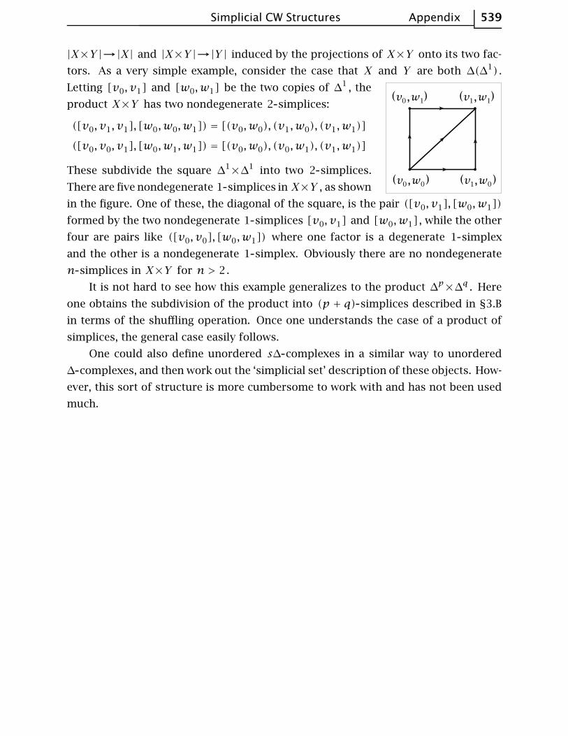
tors. As a very simple example, consider the case that X and Y are both ∆(∆1) .

Letting [v0, v1] and [w0,w1] be the two copies of ∆1 , the

product X×Y has two nondegenerate 2 simplices:

([v0, v1, v1], [w0,w0,w1]) = [(v0,w0), (v1,w0), (v1,w1)]

([v0, v0, v1], [w0,w1,w1]) = [(v0,w0), (v0,w1), (v1,w1)]

These subdivide the square ∆1×∆1 into two 2 simplices.

There are five nondegenerate 1 simplices in X×Y , as shown

in the figure. One of these, the diagonal of the square, is the pair ([v0, v1], [w0,w1])

formed by the two nondegenerate 1 simplices [v0, v1] and [w0,w1] , while the other

four are pairs like ([v0, v0], [w0,w1]) where one factor is a degenerate 1 simplex

and the other is a nondegenerate 1 simplex. Obviously there are no nondegenerate

n simplices in X×Y for n > 2.

It is not hard to see how this example generalizes to the product ∆p×∆q . Here

one obtains the subdivision of the product into (p + q) simplices described in §3.B

in terms of the shuffling operation. Once one understands the case of a product of

simplices, the general case easily follows.

One could also define unordered s∆ complexes in a similar way to unordered

∆ complexes, and then work out the ‘simplicial set’ description of these objects. How-

ever, this sort of structure is more cumbersome to work with and has not been used

much.

topology of cell complexes - cornell university

Documents