chapter 6 basics of combinatorial topologycis610/convex67.pdf · 2011-10-17 · chapter 6 basics of...

Chapter 6

Basics of Combinatorial Topology

6.1 Simplicial and Polyhedral Complexes

In order to study and manipulate complex shapes it is convenient to discretize these shapesand to view them as the union of simple building blocks glued together in a “clean fashion”.The building blocks should be simple geometric objects, for example, points, lines segments,triangles, tehrahedra and more generally simplices, or even convex polytopes. We will beginby using simplices as building blocks. The material presented in this chapter consists of themost basic notions of combinatorial topology, going back roughly to the 1900-1930 periodand it is covered in nearly every algebraic topology book (certainly the “classics”). A classictext (slightly old fashion especially for the notation and terminology) is Alexandrov [1],Volume 1 and another more “modern” source is Munkres [30]. An excellent treatment fromthe point of view of computational geometry can be found is Boissonnat and Yvinec [8],especially Chapters 7 and 10. Another fascinating book covering a lot of the basics butdevoted mostly to three-dimensional topology and geometry is Thurston [41].

Recall that a simplex is just the convex hull of a finite number of affinely independentpoints. We also need to define faces, the boundary, and the interior of a simplex.

Definition 6.1 Let E be any normed affine space, say E = Em with its usual Euclideannorm. Given any n+1 affinely independent points a0, . . . , an in E , the n-simplex (or simplex)σ defined by a0, . . . , an is the convex hull of the points a0, . . . , an, that is, the set of all convexcombinations λ0a0 + · · · + λnan, where λ0 + · · · + λn = 1 and λi ≥ 0 for all i, 0 ≤ i ≤ n.We call n the dimension of the n-simplex σ, and the points a0, . . . , an are the vertices of σ.Given any subset ai0 , . . . , aik of a0, . . . , an (where 0 ≤ k ≤ n), the k-simplex generatedby ai0 , . . . , aik is called a k-face or simply a face of σ. A face s of σ is a proper face if s = σ(we agree that the empty set is a face of any simplex). For any vertex ai, the face generatedby a0, . . . , ai−1, ai+1, . . . , an (i.e., omitting ai) is called the face opposite ai. Every face that isan (n− 1)-simplex is called a boundary face or facet . The union of the boundary faces is theboundary of σ, denoted by ∂σ, and the complement of ∂σ in σ is the interior Int σ = σ− ∂σof σ. The interior Int σ of σ is sometimes called an open simplex .

103

104 CHAPTER 6. BASICS OF COMBINATORIAL TOPOLOGY

It should be noted that for a 0-simplex consisting of a single point a0, ∂a0 = ∅, andInt a0 = a0. Of course, a 0-simplex is a single point, a 1-simplex is the line segment(a0, a1), a 2-simplex is a triangle (a0, a1, a2) (with its interior), and a 3-simplex is a tetrahe-dron (a0, a1, a2, a3) (with its interior). The inclusion relation between any two faces σ and τof some simplex, s, is written σ τ .

We now state a number of properties of simplices, whose proofs are left as an exercise.Clearly, a point x belongs to the boundary ∂σ of σ iff at least one of its barycentric co-ordinates (λ0, . . . ,λn) is zero, and a point x belongs to the interior Intσ of σ iff all of itsbarycentric coordinates (λ0, . . . ,λn) are positive, i.e., λi > 0 for all i, 0 ≤ i ≤ n. Then, forevery x ∈ σ, there is a unique face s such that x ∈ Int s, the face generated by those pointsai for which λi > 0, where (λ0, . . . ,λn) are the barycentric coordinates of x.

A simplex σ is convex, arcwise connected, compact, and closed. The interior Int σ of asimplex is convex, arcwise connected, open, and σ is the closure of Int σ.

We now put simplices together to form more complex shapes, following Munkres [30].The intuition behind the next definition is that the building blocks should be “glued cleanly”.

Definition 6.2 A simplicial complex in Em (for short, a complex in Em) is a setK consistingof a (finite or infinite) set of simplices in Em satisfying the following conditions:

(1) Every face of a simplex in K also belongs to K.

(2) For any two simplices σ1 and σ2 in K, if σ1 ∩ σ2 = ∅, then σ1 ∩ σ2 is a common face ofboth σ1 and σ2.

Every k-simplex, σ ∈ K, is called a k-face (or face) of K. A 0-face v is called a vertex anda 1-face is called an edge. The dimension of the simplicial complex K is the maximum ofthe dimensions of all simplices in K. If dimK = d, then every face of dimension d is calleda cell and every face of dimension d− 1 is called a facet .

Condition (2) guarantees that the various simplices forming a complex intersect nicely.It is easily shown that the following condition is equivalent to condition (2):

(2) For any two distinct simplices σ1, σ2, Int σ1 ∩ Int σ2 = ∅.

Remarks:

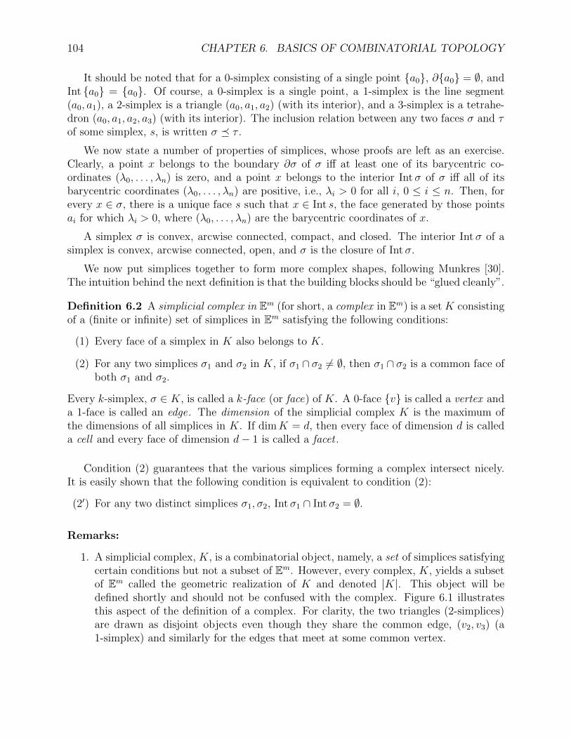
1. A simplicial complex, K, is a combinatorial object, namely, a set of simplices satisfyingcertain conditions but not a subset of Em. However, every complex, K, yields a subsetof Em called the geometric realization of K and denoted |K|. This object will bedefined shortly and should not be confused with the complex. Figure 6.1 illustratesthis aspect of the definition of a complex. For clarity, the two triangles (2-simplices)are drawn as disjoint objects even though they share the common edge, (v2, v3) (a1-simplex) and similarly for the edges that meet at some common vertex.

6.1. SIMPLICIAL AND POLYHEDRAL COMPLEXES 105 1

v1

v2

v3 v3

v2

v4

Figure 6.1: A set of simplices forming a complex1

Figure 6.2: Collections of simplices not forming a complex

2. Some authors define a facet of a complex, K, of dimension d to be a d-simplex in K,as opposed to a (d − 1)-simplex, as we did. This practice is not consistent with thenotion of facet of a polyhedron and this is why we prefer the terminology cell for thed-simplices in K.

3. It is important to note that in order for a complex, K, of dimension d to be realized inEm, the dimension of the “ambient space”, m, must be big enough. For example, thereare 2-complexes that can’t be realized in E3 or even in E4. There has to be enoughroom in order for condition (2) to be satisfied. It is not hard to prove that m = 2d+1is always sufficient. Sometimes, 2d works, for example in the case of surfaces (whered = 2).

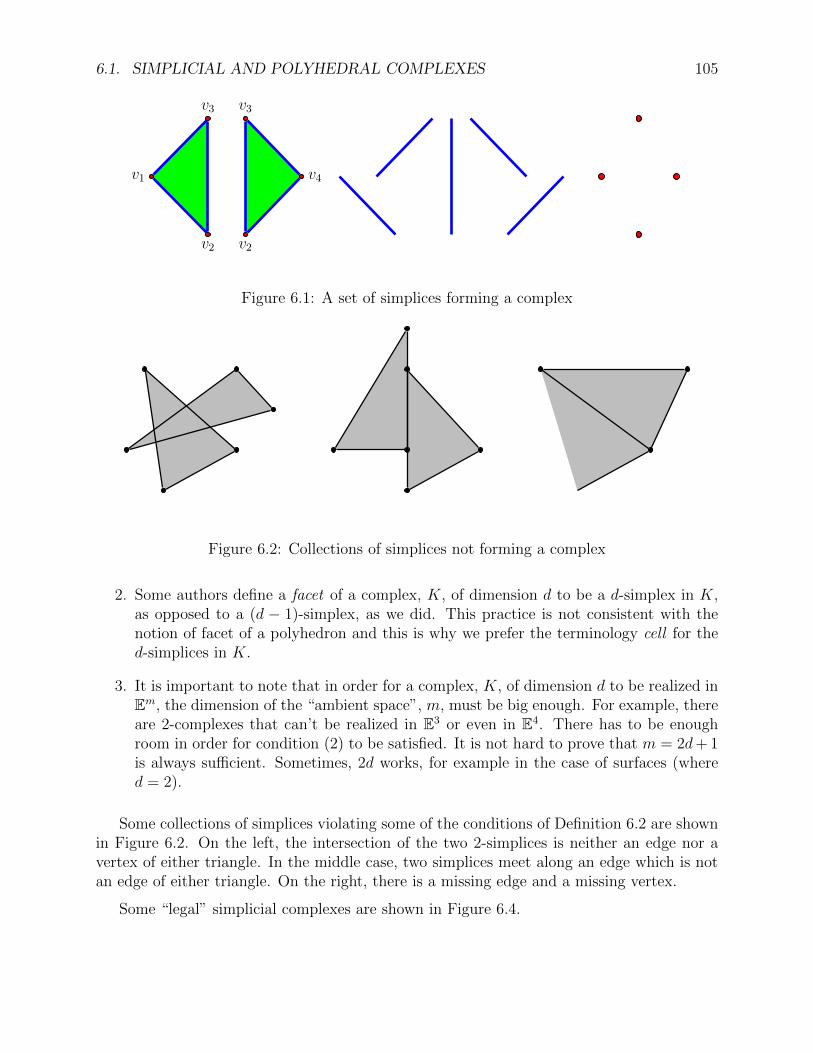
Some collections of simplices violating some of the conditions of Definition 6.2 are shownin Figure 6.2. On the left, the intersection of the two 2-simplices is neither an edge nor avertex of either triangle. In the middle case, two simplices meet along an edge which is notan edge of either triangle. On the right, there is a missing edge and a missing vertex.

Some “legal” simplicial complexes are shown in Figure 6.4.

106 CHAPTER 6. BASICS OF COMBINATORIAL TOPOLOGY 1

v1

v2

v3

v4

Figure 6.3: The geometric realization of the complex of Figure 6.1 1

Figure 6.4: Examples of simplicial complexes

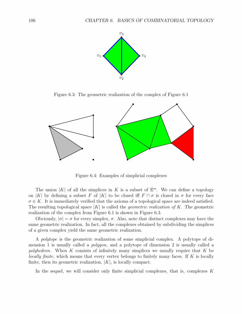
The union |K| of all the simplices in K is a subset of Em. We can define a topologyon |K| by defining a subset F of |K| to be closed iff F ∩ σ is closed in σ for every faceσ ∈ K. It is immediately verified that the axioms of a topological space are indeed satisfied.The resulting topological space |K| is called the geometric realization of K. The geometricrealization of the complex from Figure 6.1 is shown in Figure 6.3.

Obviously, |σ| = σ for every simplex, σ. Also, note that distinct complexes may have thesame geometric realization. In fact, all the complexes obtained by subdividing the simplicesof a given complex yield the same geometric realization.

A polytope is the geometric realization of some simplicial complex. A polytope of di-mension 1 is usually called a polygon, and a polytope of dimension 2 is usually called apolyhedron. When K consists of infinitely many simplices we usually require that K belocally finite, which means that every vertex belongs to finitely many faces. If K is locallyfinite, then its geometric realization, |K|, is locally compact.

In the sequel, we will consider only finite simplicial complexes, that is, complexes K


(a) (b)

v

Figure 6.5: (a) A complex that is not pure. (b) A pure complex

consisting of a finite number of simplices. In this case, the topology of |K| defined aboveis identical to the topology induced from Em. Also, for any simplex σ in K, Int σ coincideswith the interior

σ of σ in the topological sense, and ∂σ coincides with the boundary of σ in

the topological sense.

Definition 6.3 Given any complex, K2, a subset K1 ⊆ K2 of K2 is a subcomplex of K2 iff itis also a complex. For any complex, K, of dimension d, for any i with 0 ≤ i ≤ d, the subset

K(i) = σ ∈ K | dim σ ≤ i

is called the i-skeleton of K. Clearly, K(i) is a subcomplex of K. We also let

Ki = σ ∈ K | dim σ = i.

Observe that K0 is the set of vertices of K and Ki is not a complex. A simplicial complex,K1 is a subdivision of a complex K2 iff |K1| = |K2| and if every face of K1 is a subset ofsome face of K2. A complex K of dimension d is pure (or homogeneous) iff every face ofK is a face of some d-simplex of K (i.e., some cell of K). A complex is connected iff |K| isconnected.

It is easy to see that a complex is connected iff its 1-skeleton is connected. The intuitionbehind the notion of a pure complex, K, of dimension d is that a pure complex is the resultof gluing pieces all having the same dimension, namely, d-simplices. For example, in Figure6.5, the complex on the left is not pure but the complex on the right is pure of dimension 2.

Most of the shapes that we will be interested in are well approximated by pure com-plexes, in particular, surfaces or solids. However, pure complexes may still have undesirable“singularities” such as the vertex, v, in Figure 6.5(b). The notion of link of a vertex providesa technical way to deal with singularities.

108 CHAPTER 6. BASICS OF COMBINATORIAL TOPOLOGY 1

(a)

v

(b)

v

Figure 6.6: (a) A complex. (b) Star and Link of v

Definition 6.4 Let K be any complex and let σ be any face of K. The star , St(σ) (or ifwe need to be very precise, St(σ, K)), of σ is the subcomplex of K consisting of all faces, τ ,containing σ and of all faces of τ , i.e.,

St(σ) = s ∈ K | (∃τ ∈ K)(σ τ and s τ).

The link , Lk(σ) (or Lk(σ, K)) of σ is the subcomplex of K consisting of all faces in St(σ)that do not intersect σ, i.e.,

Lk(σ) = τ ∈ K | τ ∈ St(σ) and σ ∩ τ = ∅.

To simplify notation, if σ = v is a vertex we write St(v) for St(v) and Lk(v) forLk(v). Figure 6.6 shows:

(a) A complex (on the left).

(b) The star of the vertex v, indicated in gray and the link of v, shown as thicker lines.

If K is pure and of dimension d, then St(σ) is also pure of dimension d and if dim σ = k,then Lk(σ) is pure of dimension d− k − 1.

For technical reasons, following Munkres [30], besides defining the complex, St(σ), it isuseful to introduce the open star of σ, denoted st(σ), defined as the subspace of |K| consistingof the union of the interiors, Int(τ) = τ − ∂ τ , of all the faces, τ , containing, σ. Accordingto this definition, the open star of σ is not a complex but instead a subset of |K|.

Note thatst(σ) = |St(σ)|,

6.1. SIMPLICIAL AND POLYHEDRAL COMPLEXES 109

that is, the closure of st(σ) is the geometric realization of the complex St(σ). Then,lk(σ) = |Lk(σ)| is the union of the simplices in St(σ) that are disjoint from σ. If σ is avertex, v, we have

lk(v) = st(v)− st(v).

However, beware that if σ is not a vertex, then lk(σ) is properly contained in st(σ)− st(σ)!

One of the nice properties of the open star, st(σ), of σ is that it is open. To see this,observe that for any point, a ∈ |K|, there is a unique smallest simplex, σ = (v0, . . . , vk), suchthat a ∈ Int(σ), that is, such that

a = λ0v0 + · · ·+ λkvk

with λi > 0 for all i, with 0 ≤ i ≤ k (and of course, λ0 + · · · + λk = 1). (When k = 0, wehave v0 = a and λ0 = 1.) For every arbitrary vertex, v, of K, we define tv(a) by

tv(a) =

λi if v = vi, with 0 ≤ i ≤ k,0 if v /∈ v0, . . . , vk.

Using the above notation, observe that

st(v) = a ∈ |K| | tv(a) > 0and thus, |K| − st(v) is the union of all the faces of K that do not contain v as a vertex,obviously a closed set. Thus, st(v) is open in |K|. It is also quite clear that st(v) is pathconnected. Moreover, for any k-face, σ, of K, if σ = (v0, . . . , vk), then

st(σ) = a ∈ |K| | tvi(a) > 0, 0 ≤ i ≤ k,that is,

st(σ) = st(v0) ∩ · · · ∩ st(vk).

Consequently, st(σ) is open and path connected. Unfortunately, the “nice” equation

St(σ) = St(v0) ∩ · · · ∩ St(vk)

is false! (and anagolously for Lk(σ).) For a counter-example, consider the boundary of atetrahedron with one face removed.

Recall that in Ed, the (open) unit ball, Bd, is defined by

Bd = x ∈ Ed | x < 1,

the closed unit ball, Bd

, is defined by

Bd

= x ∈ Ed | x ≤ 1,and the (d− 1)-sphere, Sd−1, by

Sd−1 = x ∈ Ed | x = 1.

Obviously, Sd−1 is the boundary of Bd

(and Bd).


Definition 6.5 Let K be a pure complex of dimension d and let σ be any k-face of K, with0 ≤ k ≤ d− 1. We say that σ is nonsingular iff the geometric realization, lk(σ), of the link

of σ is homeomorphic to either Sd−k−1 or to Bd−k−1

; this is written as lk(σ) ≈ Sd−k−1 or

lk(σ) ≈ Bd−k−1

, where ≈ means homeomorphic.

In Figure 6.6, note that the link of v is not homeomorphic to S1 or B1, so v is singular.

It will also be useful to express St(v) in terms of Lk(v), where v is a vertex, and for this,we define yet another notion of cone.

Definition 6.6 Given any complex, K, in En, if dimK = d < n, for any point, v ∈ En,such that v does not belong to the affine hull of |K|, the cone on K with vertex v, denoted,v ∗ K, is the complex consisting of all simplices of the form (v, a0, . . . , ak) and their faces,where (a0, . . . , ak) is any k-face of K. If K = ∅, we set v ∗K = v.

It is not hard to check that v ∗K is indeed a complex of dimension d + 1 containing Kas a subcomplex.

Remark: Unfortunately, the word “cone” is overloaded. It might have been better to usethe locution pyramid instead of cone as some authors do (for example, Ziegler). However,since we have been following Munkres [30], a standard reference in algebraic topology, wedecided to stick with the terminology used in that book, namely, “cone”.

The following proposition is also easy to prove:

Proposition 6.1 For any complex, K, of dimension d and any vertex, v ∈ K, we have

St(v) = v ∗ Lk(v).

More generally, for any face, σ, of K, we have

st(σ) = |St(σ)| ≈ σ × |v ∗ Lk(σ)|,

for every v ∈ σ andst(σ)− st(σ) = ∂ σ × |v ∗ Lk(σ)|,

for every v ∈ ∂ σ.

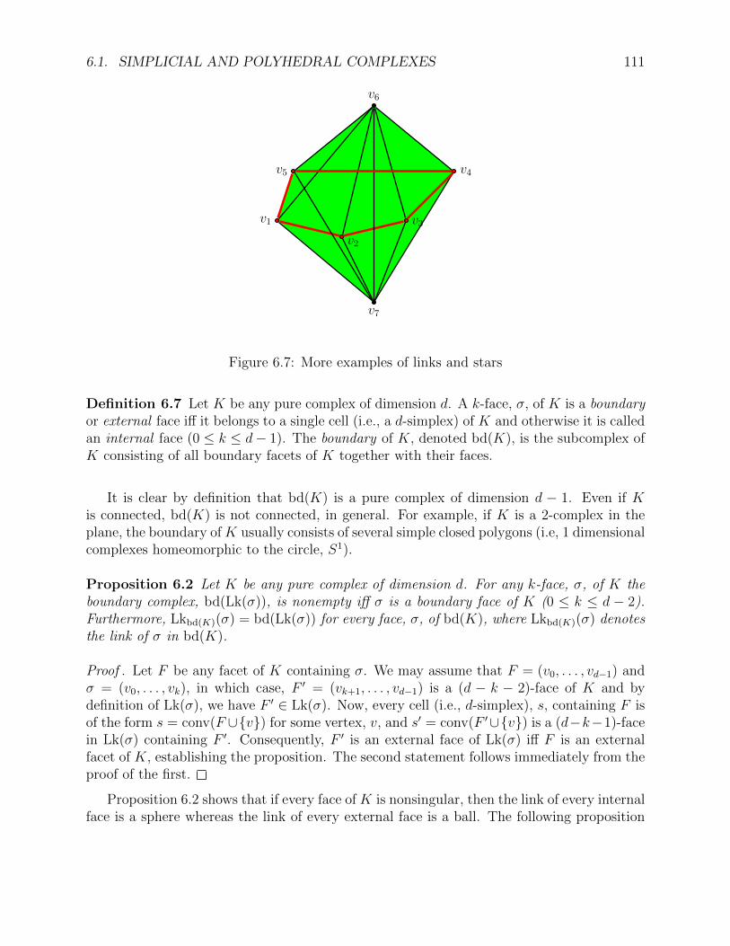
Figure 6.7 shows a 3-dimensional complex. The link of the edge (v6, v7) is the pentagonP = (v1, v2, v3, v4, v5) ≈ S1. The link of the vertex v7 is the cone v6 ∗ P ≈ B2. The linkof (v1, v2) is (v6, v7) ≈ B1 and the link of v1 is the union of the triangles (v2, v6, v7) and(v5, v6, v7), which is homeomorphic to B2.

Given a pure complex, it is necessary to distinguish between two kinds of faces.


v1

v2

v3

v4v5

v6

v7

Figure 6.7: More examples of links and stars

Definition 6.7 Let K be any pure complex of dimension d. A k-face, σ, of K is a boundaryor external face iff it belongs to a single cell (i.e., a d-simplex) of K and otherwise it is calledan internal face (0 ≤ k ≤ d− 1). The boundary of K, denoted bd(K), is the subcomplex ofK consisting of all boundary facets of K together with their faces.

It is clear by definition that bd(K) is a pure complex of dimension d − 1. Even if Kis connected, bd(K) is not connected, in general. For example, if K is a 2-complex in theplane, the boundary ofK usually consists of several simple closed polygons (i.e, 1 dimensionalcomplexes homeomorphic to the circle, S1).

Proposition 6.2 Let K be any pure complex of dimension d. For any k-face, σ, of K theboundary complex, bd(Lk(σ)), is nonempty iff σ is a boundary face of K (0 ≤ k ≤ d − 2).Furthermore, Lkbd(K)(σ) = bd(Lk(σ)) for every face, σ, of bd(K), where Lkbd(K)(σ) denotesthe link of σ in bd(K).

Proof . Let F be any facet of K containing σ. We may assume that F = (v0, . . . , vd−1) andσ = (v0, . . . , vk), in which case, F = (vk+1, . . . , vd−1) is a (d − k − 2)-face of K and bydefinition of Lk(σ), we have F ∈ Lk(σ). Now, every cell (i.e., d-simplex), s, containing F isof the form s = conv(F ∪v) for some vertex, v, and s = conv(F ∪v) is a (d−k−1)-facein Lk(σ) containing F . Consequently, F is an external face of Lk(σ) iff F is an externalfacet of K, establishing the proposition. The second statement follows immediately from theproof of the first.

Proposition 6.2 shows that if every face ofK is nonsingular, then the link of every internalface is a sphere whereas the link of every external face is a ball. The following proposition


shows that for any pure complex, K, nonsingularity of all the vertices is enough to implythat every open star is homeomorphic to Bd:

Proposition 6.3 Let K be any pure complex of dimension d. If every vertex of K is non-singular, then st(σ) ≈ Bd for every k-face, σ, of K (1 ≤ k ≤ d− 1).

Proof . Let σ be any k-face of K and assume that σ is generated by the vertices v0, . . . , vk,

with 1 ≤ k ≤ d − 1. By hypothesis, lk(vi) is homeomorphic to either Sd−1 or Bd−1

. Then,it is easy to show that in either case, we have

|vi ∗ Lk(vi)| ≈ Bd

,

and by Proposition 6.1, we get

|St(vi)| ≈ Bd

.

Consequently, st(vi) ≈ Bd. Furthermore,

st(σ) = st(v0) ∩ · · · ∩ st(vk) ≈ Bd

and so, st(σ) ≈ Bd, as claimed.

Here are more useful propositions about pure complexes without singularities.

Proposition 6.4 Let K be any pure complex of dimension d. If every vertex of K is non-singular, then for every point, a ∈ |K|, there is an open subset, U ⊆ |K|, containing a suchthat U ≈ Bd or U ≈ Bd ∩Hd, where Hd = (x1, . . . , xd) ∈ Rd | xd ≥ 0.

Proof . We already know from Proposition 6.3 that st(σ) ≈ Bd, for every σ ∈ K. So, if a ∈ σand σ is not a boundary face, we can take U = st(σ) ≈ Bd. If σ is a boundary face, then|σ| ⊆ |bd(St(σ))| and it can be shown that we can take U = Bd ∩Hd.

Proposition 6.5 Let K be any pure complex of dimension d. If every facet of K is nonsin-gular, then every facet of K, is contained in at most two cells (d-simplices).

Proof . If |K| ⊆ Ed, then this is an immediate consequence of the definition of a complex.Otherwise, consider lk(σ). By hypothesis, either lk(σ) ≈ B0 or lk(σ) ≈ S0. As B0 = 0,S0 = −1, 1 and dimLk(σ) = 0, we deduce that Lk(σ) has either one or two points, whichproves that σ belongs to at most two d-simplices.

Proposition 6.6 Let K be any pure and connected complex of dimension d. If every face ofK is nonsingular, then for every pair of cells (d-simplices), σ and σ, there is a sequence ofcells, σ0, . . . , σp, with σ0 = σ and σp = σ, and such that σi and σi+1 have a common facet,for i = 0, . . . , p− 1.

Proof . We proceed by induction on d, using the fact that the links are connected for d ≥ 2.

6.1. SIMPLICIAL AND POLYHEDRAL COMPLEXES 113

Proposition 6.7 Let K be any pure complex of dimension d. If every facet of K is nonsin-gular, then the boundary, bd(K), of K is a pure complex of dimension d− 1 with an emptyboundary. Furthermore, if every face of K is nonsingular, then every face of bd(K) is alsononsingular.

Proof . Left as an exercise.

The building blocks of simplicial complexes, namely, simplicies, are in some sense math-ematically ideal. However, in practice, it may be desirable to use a more flexible set ofbuilding blocks. We can indeed do this and use convex polytopes as our building blocks.

Definition 6.8 A polyhedral complex in Em (for short, a complex in Em) is a set, K, consist-ing of a (finite or infinite) set of convex polytopes in Em satisfying the following conditions:

(1) Every face of a polytope in K also belongs to K.

(2) For any two polytopes σ1 and σ2 in K, if σ1 ∩ σ2 = ∅, then σ1 ∩ σ2 is a common faceof both σ1 and σ2.

Every polytope, σ ∈ K, of dimension k, is called a k-face (or face) of K. A 0-face v iscalled a vertex and a 1-face is called an edge. The dimension of the polyhedral complex Kis the maximum of the dimensions of all polytopes in K. If dimK = d, then every face ofdimension d is called a cell and every face of dimension d− 1 is called a facet .

Remark: Since the building blocks of a polyhedral complex are convex polytopes it mightbe more appropriate to use the term “polytopal complex” rather than “polyhedral complex”and some authors do that. On the other hand, most of the traditional litterature uses theterminology polyhedral complex so we will stick to it. There is a notion of complex wherethe building blocks are cones but these are called fans .

Every convex polytope, P , yields two natural polyhedral complexes:

(i) The polyhedral complex, K(P ), consisting of P together with all of its faces. Thiscomplex has a single cell, namely, P itself.

(ii) The boundary complex , K(∂P ), consisting of all faces of P other than P itself. Thecells of K(∂P ) are the facets of P .

The notions of k-skeleton and pureness are defined just as in the simplicial case. Thenotions of star and link are defined for polyhedral complexes just as they are defined forsimplicial complexes except that the word “face” now means face of a polytope. Now, byTheorem 4.7, every polytope, σ, is the convex hull of its vertices. Let vert(σ) denote theset of vertices of σ. Then, we have the following crucial observation: Given any polyhedralcomplex, K, for every point, x ∈ |K|, there is a unique polytope, σx ∈ K, such thatx ∈ Int(σx) = σx − ∂ σx. We define a function, t : V → R+, that tests whether x belongs to


the interior of any face (polytope) of K having v as a vertex as follows: For every vertex, v,of K,

tv(x) =

1 if v ∈ vert(σx)0 if v /∈ vert(σx),

where σx is the unique face of K such that x ∈ Int(σx).

Now, just as in the simplicial case, the open star, st(v), of a vertex, v ∈ K, is given by

st(v) = x ∈ |K| | tv(x) = 1and it is an open subset of |K| (the set |K|− st(v) is the union of the polytopes of K thatdo not contain v as a vertex, a closed subset of |K|). Also, for any face, σ, of K, the openstar, st(σ), of σ is given by

st(σ) = x ∈ |K| | tv(x) = 1, for all v ∈ vert(σ) =

v∈vert(σ)st(v).

Therefore, st(σ) is also open in |K|.The next proposition is another result that seems quite obvious, yet a rigorous proof

is more involved that we might think. This proposition states that a convex polytope canalways be cut up into simplices, that is, it can be subdivided into a simplicial complex.In other words, every convex polytope can be triangulated. This implies that simplicialcomplexes are as general as polyhedral complexes.

One should be warned that even though, in the plane, every bounded region (not nec-essarily convex) whose boundary consists of a finite number of closed polygons (polygonshomeomorphic to the circle, S1) can be triangulated, this is no longer true in three dimen-sions!

Proposition 6.8 Every convex d-polytope, P , can be subdivided into a simplicial complexwithout adding any new vertices, i.e., every convex polytope can be triangulated.

Proof sketch. It would be tempting to proceed by induction on the dimension, d, of P butwe do not know any correct proof of this kind. Instead, we proceed by induction on thenumber, p, of vertices of P . Since dim(P ) = d, we must have p ≥ d+ 1. The case p = d+ 1corresponds to a simplex, so the base case holds.

For p > d + 1, we can pick some vertex, v ∈ P , such that the convex hull, Q, of theremaining p − 1 vertices still has dimension d. Then, by the induction hypothesis, Q, hasa simplicial subdivision. Now, we say that a facet, F , of Q is visible from v iff v and theinterior of Q are strictly separated by the supporting hyperplane of F . Then, we add thed-simplices, conv(F ∪ v) = v ∗ F , for every facet, F , of Q visible from v to those in thetriangulation of Q. We claim that the resulting collection of simplices (with their faces)constitutes a simplicial complex subdividing P . This is the part of the proof that requiresa careful and somewhat tedious case analysis, which we omit. However, the reader shouldcheck that everything really works out!

With all this preparation, it is now quite natural to define combinatorial manifolds.

6.2. COMBINATORIAL AND TOPOLOGICAL MANIFOLDS 115

6.2 Combinatorial and Topological Manifolds

The notion of pure complex without singular faces turns out to be a very good “discrete”approximation of the notion of (topological) manifold because of its highly computationalnature. This motivates the following definition:

Definition 6.9 A combinatorial d-manifold is any space,X, homeomorphic to the geometricrealization, |K| ⊆ En, of some pure (simplicial or polyhedral) complex, K, of dimension dwhose faces are all nonsingular. If the link of every k-face of K is homeomorphic to thesphere Sd−k−1, we say that X is a combinatorial manifold without boundary , else it is acombinatorial manifold with boundary .

Other authors use the term triangulation for what we call a combinatorial manifold.

It is easy to see that the connected components of a combinatorial 1-manifold are eithersimple closed polygons or simple chains (“simple” means that the interiors of distinct edgesare disjoint). A combinatorial 2-manifold which is connected is also called a combinatorialsurface (with or without boundary). Proposition 6.7 immediately yields the following result:

Proposition 6.9 If X is a combinatorial d-manifold with boundary, then bd(X) is a com-binatorial (d− 1)-manifold without boundary.

Now, because we are assuming that X sits in some Euclidean space, En, the space Xis Hausdorff and second-countable. (Recall that a topological space is second-countable iffthere is a countable family, Uii≥0, of open sets of X such that every open subset of X isthe union of open sets from this family.) Since it is desirable to have a good match betweenmanifolds and combinatorial manifolds, we are led to the definition below.

Recall thatHd = (x1, . . . , xd) ∈ Rd | xd ≥ 0.

Definition 6.10 For any d ≥ 1, a (topological) d-manifold with boundary is a second-countable, topological Hausdorff space M , together with an open cover, (Ui)i∈I , of opensets in M and a family, (ϕi)i∈I , of homeomorphisms, ϕi : Ui → Ωi, where each Ωi is someopen subset of Hd in the subset topology. Each pair (U,ϕ) is called a coordinate system, orchart , of M , each homeomorphism ϕi : Ui → Ωi is called a coordinate map, and its inverseϕ−1i

: Ωi → Ui is called a parameterization of Ui. The family (Ui,ϕi)i∈I is often called anatlas for M . A (topological) bordered surface is a connected 2-manifold with boundary. Iffor every homeomorphism, ϕi : Ui → Ωi, the open set Ωi ⊆ Hd is actually an open set in Rd

(which means that xd > 0 for every (x1, . . . , xd) ∈ Ωi), then we say that M is a d-manifold .

Note that a d-manifold is also a d-manifold with boundary.

If ϕi : Ui → Ωi is some homeomorphism onto some open set Ωi of Hd in the subsettopology, some p ∈ Ui may be mapped into Rd−1 × R+, or into the “boundary” Rd−1 × 0


of Hd. Letting ∂Hd = Rd−1 × 0, it can be shown using homology that if some coordinatemap, ϕ, defined on p maps p into ∂Hd, then every coordinate map, ψ, defined on p maps pinto ∂Hd.

Thus,M is the disjoint union of two sets ∂M and IntM , where ∂M is the subset consistingof all points p ∈ M that are mapped by some (in fact, all) coordinate map, ϕ, defined onp into ∂Hd, and where IntM = M − ∂M . The set ∂M is called the boundary of M , andthe set IntM is called the interior of M , even though this terminology clashes with someprior topological definitions. A good example of a bordered surface is the Mobius strip. Theboundary of the Mobius strip is a circle.

The boundary ∂M of M may be empty, but IntM is nonempty. Also, it can be shownusing homology that the integer d is unique. It is clear that IntM is open and a d-manifold,and that ∂M is closed. If p ∈ ∂M , and ϕ is some coordinate map defined on p, since Ω = ϕ(U)is an open subset of ∂Hd, there is some open half ball Bd

o+ centered at ϕ(p) and contained inΩ which intersects ∂Hd along an open ball Bd−1

o, and if we consider W = ϕ−1(Bd

o+), we havean open subset of M containing p which is mapped homeomorphically onto Bd

o+ in such thatway that every point in W ∩ ∂M is mapped onto the open ball Bd−1

o. Thus, it is easy to see

that ∂M is a (d− 1)-manifold.

Proposition 6.10 Every combinatorial d-manifold is a d-manifold with boundary.

Proof . This is an immediate consequence of Proposition 6.4.

Is the converse of Proposition 6.10 true?

It turns out that answer is yes for d = 1, 2, 3 but no for d ≥ 4. This is not hard toprove for d = 1. For d = 2 and d = 3, this is quite hard to prove; among other things, it isnecessary to prove that triangulations exist and this is very technical. For d ≥ 4, not everymanifold can be triangulated (in fact, this is undecidable!).

What if we assume that M is a triangulated manifold, which means that M ≈ |K|, forsome pure d-dimensional complex, K?

Surprisingly, for d ≥ 5, there are triangulated manifolds whose links are not spherical

(i.e., not homeomorphic to Bd−k−1

or Sd−k−1), see Thurston [41].

Fortunately, we will only have to deal with d = 2, 3! Another issue that must be addressedis orientability.

Assume that we fix a total ordering of the vertices of a complex, K. Let σ = (v0, . . . , vk)be any simplex. Recall that every permutation (of 0, . . . , k) is a product of transpositions ,where a transposition swaps two distinct elements, say i and j, and leaves every other elementfixed. Furthermore, for any permutation, π, the parity of the number of transpositionsneeded to obtain π only depends on π and it called the signature of π. We say that twopermutations are equivalent iff they have the same signature. Consequently, there are twoequivalence classes of permutations: Those of even signature and those of odd signature.

6.2. COMBINATORIAL AND TOPOLOGICAL MANIFOLDS 117

Then, an orientation of σ is the choice of one of the two equivalence classes of permutationsof its vertices. If σ has been given an orientation, then we denote by −σ the result ofassigning the other orientation to it (we call it the opposite orientation).

For example, (0, 1, 2) has the two orientation classes:

(0, 1, 2), (1, 2, 0), (2, 0, 1) and (2, 1, 0), (1, 0, 2), (0, 2, 1).

Definition 6.11 Let X ≈ |K| be a combinatorial d-manifold. We say that X is orientableif it is possible to assign an orientation to all of its cells (d-simplices) so that whenever twocells σ1 and σ2 have a common facet, σ, the two orientations induced by σ1 and σ2 on σ areopposite. A combinatorial d-manifold together with a specific orientation of its cells is calledan oriented manifold . If X is not orientable we say that it is non-orientable.

Remark: It is possible to define the notion of orientation of a manifold but this is quitetechnical and we prefer to avoid digressing into this matter. This shows another advantageof combinatorial manifolds: The definition of orientability is simple and quite natural.

There are non-orientable (combinatorial) surfaces, for example, the Mobius strip whichcan be realized in E3. The Mobius strip is a surface with boundary, its boundary being acircle. There are also non-orientable (combinatorial) surfaces such as the Klein bottle orthe projective plane but they can only be realized in E4 (in E3, they must have singularitiessuch as self-intersection). We will only be dealing with orientable manifolds and, most ofthe time, surfaces.

One of the most important invariants of combinatorial (and topological) manifolds istheir Euler(-Poincare) characteristic. In the next chapter, we prove a famous formula dueto Poincare giving the Euler characteristic of a convex polytope. For this, we will introducea technique of independent interest called shelling .

Chapter 7

Shellings, the Euler-Poincare Formulafor Polytopes, the Dehn-SommervilleEquations and the Upper BoundTheorem

7.1 Shellings

The notion of shellability is motivated by the desire to give an inductive proof of the Euler-Poincare formula in any dimension. Historically, this formula was discovered by Euler forthree dimensional polytopes in 1752 (but it was already known to Descartes around 1640).If f0, f1 and f2 denote the number of vertices, edges and triangles of the three dimensionalpolytope, P , (i.e., the number of i-faces of P for i = 0, 1, 2), then the Euler formula statesthat

f0 − f1 + f2 = 2.

The proof of Euler’s formula is not very difficult but one still has to exercise caution. Euler’sformula was generalized to arbitrary d-dimensional polytopes by Schlafli (1852) but thefirst correct proof was given by Poincare. For this, Poincare had to lay the foundations ofalgebraic topology and after a first “proof” given in 1893 (containing some flaws) he finallygave the first correct proof in 1899. If fi denotes the number of i-faces of the d-dimensionalpolytope, P , (with f−1 = 1 and fd = 1), the Euler-Poincare formula states that:

d−1

i=0

(−1)ifi = 1− (−1)d,

which can also be written asd

i=0

(−1)ifi = 1,

119

120 CHAPTER 7. SHELLINGS AND THE EULER-POINCARE FORMULA

by incorporating fd = 1 in the first formula or as

d

i=−1

(−1)ifi = 0,

by incorporating both f−1 = 1 and fd = 1 in the first formula.

Earlier inductive “proofs” of the above formula were proposed, notably a proof by Schlafliin 1852, but it was later observed that all these proofs assume that the boundary of everypolytope can be built up inductively in a nice way, what is called shellability . Actually,counter-examples of shellability for various simplicial complexes suggested that polytopeswere perhaps not shellable. However, the fact that polytopes are shellable was finally provedin 1970 by Bruggesser and Mani [12] and soon after that (also in 1970) a striking applicationof shellability was made by McMullen [29] who gave the first proof of the so-called “upperbound theorem”.

As shellability of polytopes is an important tool and as it yields one of the cleanestinductive proof of the Euler-Poincare formula, we will sketch its proof in some details. ThisChapter is heavily inspired by Ziegler’s excellent treatment [45], Chapter 8. We begin withthe definition of shellability. It’s a bit technical, so please be patient!

Definition 7.1 Let K be a pure polyhedral complex of dimension d. A shelling of K is alist, F1, . . . , Fs, of the cells (i.e., d-faces) of K such that either d = 0 (and thus, all Fi arepoints) or the following conditions hold:

(i) The boundary complex, K(∂F1), of the first cell, F1, of K has a shelling.

(ii) For any j, 1 < j ≤ s, the intersection of the cell Fj with the previous cells is nonemptyand is an initial segment of a shelling of the (d− 1)-dimensional boundary complex ofFj, that is

Fj ∩

j−1

i=1

Fi

= G1 ∪G2 ∪ · · · ∪Gr,

for some shelling G1, G2, . . . , Gr, . . . , Gt of K(∂Fj), with 1 ≤ r ≤ t. As the intersectionshould be the initial segment of a shelling for the (d− 1)-dimensional complex, ∂Fj, ithas to be pure (d− 1)-dimensional and connected for d > 1.

A polyhedral complex is shellable if it is pure and has a shelling.

Note that shellabiliy is only defined for pure complexes. Here are some examples ofshellable complexes:

(1) Every 0-dimensional complex, that is, evey set of points, is shellable, by definition.

7.1. SHELLINGS 121 1

1

21 2 3

4

567

8

1

2

34 5

Figure 7.1: Non shellable and Shellable 2-complexes

(2) A 1-dimensional complex is a graph without loops and parallel edges. A 1-dimensionalcomplex is shellable iff it is connected, which implies that it has no isolated vertices.Any ordering of the edges, e1, . . . , es, such that e1, . . . , ei induces a connected sub-graph for every i will do. Such an ordering can be defined inductively, due to theconnectivity of the graph.

(3) Every simplex is shellable. In fact, any ordering of its facets yields a shelling. This iseasily shown by induction on the dimension, since the intersection of any two facets Fi

and Fj is a facet of both Fi and Fj.

(4) The d-cubes are shellable. By induction on the dimension, it can be shown thatevery ordering of the 2d facets F1, . . . , F2d such that F1 and F2d are opposite (that is,F2d = −F1) yields a shelling.

However, already for 2-complexes, problems arise. For example, in Figure 7.1, the leftand the middle 2-complexes are not shellable but the right complex is shellable.

The problem with the left complex is that cells 1 and 2 intersect at a vertex, which is not1-dimensional, and in the middle complex, the intersection of cell 8 with its predecessors isnot connected. In contrast, the ordering of the right complex is a shelling. However, observethat the reverse ordering is not a shelling because cell 4 has an empty intersection with cell5!

Remarks:

1. Condition (i) in Definition 7.1 is redundant because, as we shall prove shortly, everypolytope is shellable. However, if we want to use this definition for more generalcomplexes, then condition (i) is necessary.

2. When K is a simplicial complex, condition (i) is of course redundant, as every simplexis shellable but condition (ii) can also be simplified to:

(ii’) For any j, with 1 < j ≤ s, the intersection of Fj with the previous cells isnonempty and pure (d− 1)-dimensional. This means that for every i < j there issome l < j such that Fi ∩ Fj ⊆ Fl ∩ Fj and Fl ∩ Fj is a facet of Fj.


The following proposition yields an important piece of information about the local struc-ture of shellable simplicial complexes:

Proposition 7.1 Let K be a shellable simplicial complex and say F1, . . . , Fs is a shellingfor K. Then, for every vertex, v, the restriction of the above sequence to the link, Lk(v),and to the star, St(v), are shellings.

Since the complex, K(P ), associated with a polytope, P , has a single cell, namely P itself,note that by condition (i) in the definition of a shelling, K(P ) is shellable iff the complex,K(∂P ), is shellable. We will say simply say that “P is shellable” instead of “K(∂P ) isshellable”.

We have the following useful property of shellings of polytopes whose proof is left as anexercise (use induction on the dimension):

Proposition 7.2 Given any polytope, P , if F1, . . . , Fs is a shelling of P , then the reversesequence Fs, . . . , F1 is also a shelling of P .

Proposition 7.2 generally fails for complexes that are not polytopes, see the right 2-complex in Figure 7.1.

We will now present the proof that every polytope is shellable, using a technique inventedby Bruggesser and Mani (1970) known as line shelling [12]. This is quite a simple andnatural idea if one is willing to ignore the technical details involved in actually checking thatit works. We begin by explaining this idea in the 2-dimensional case, a convex polygon, sinceit is particularly simple.

Consider the 2-polytope, P , shown in Figure 7.2 (a polygon) whose faces are labeledF1, F2, F3, F4, F5. Pick any line, , intersecting the interior of P and intersecting the sup-porting lines of the facets of P (i.e., the edges of P ) in distinct points labeled z1, z2, z3, z4, z5(such a line can always be found, as will be shown shortly). Orient the line, , (say, upward)and travel on starting from the point of P where leaves P , namely, z1. For a while, onlyface F1 is visible but when we reach the intersection, z2, of with the supporting line of F2,the face F2 becomes visible and F1 becomes invisible as it is now hidden by the supportingline of F2. So far, we have seen the faces, F1 and F2, in that order . As we continue travelingalong , no new face becomes visible but for a more complicated polygon, other faces, Fi,would become visible one at a time as we reach the intersection, zi, of with the supportingline of Fi and the order in which these faces become visible corresponds to the ordering of thezi’s along the line . Then, we imagine that we travel very fast and when we reach “+∞” inthe upward direction on , we instantly come back on from below at “−∞”. At this point,we only see the face of P corresponding to the lowest supporting line of faces of P , i.e., theline corresponding to the smallest zi, in our case, z3. At this stage, the only visible face isF3. We continue traveling upward on and we reach z3, the intersection of the supportingline of F3 with . At this moment, F4 becomes visible and F3 disappears as it is now hidden

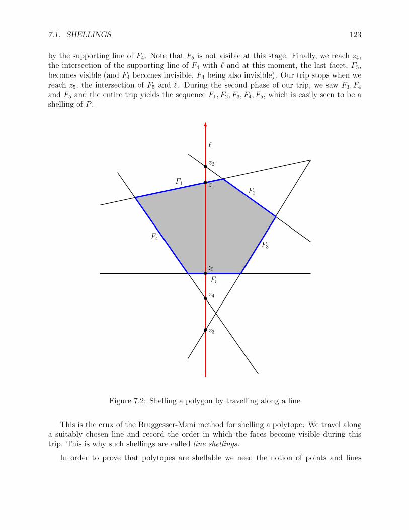
7.1. SHELLINGS 123

by the supporting line of F4. Note that F5 is not visible at this stage. Finally, we reach z4,the intersection of the supporting line of F4 with and at this moment, the last facet, F5,becomes visible (and F4 becomes invisible, F3 being also invisible). Our trip stops when wereach z5, the intersection of F5 and . During the second phase of our trip, we saw F3, F4

and F5 and the entire trip yields the sequence F1, F2, F3, F4, F5, which is easily seen to be ashelling of P . 1

F1

F2

F3

F5

F4

z1

z2

z3

z4

z5

Figure 7.2: Shelling a polygon by travelling along a line

This is the crux of the Bruggesser-Mani method for shelling a polytope: We travel alonga suitably chosen line and record the order in which the faces become visible during thistrip. This is why such shellings are called line shellings .

In order to prove that polytopes are shellable we need the notion of points and lines


in “general position”. Recall from the equivalence of V-polytopes and H-polytopes that apolytope, P , in Ed with nonempty interior is cut out by t irredundant hyperplanes, Hi, andby picking the origin in the interior of P the equations of the Hi may be assumed to be ofthe form

ai · z = 1

where ai and aj are not proportional for all i = j, so that

P = z ∈ Ed | ai · z ≤ 1, 1 ≤ i ≤ t.

Definition 7.2 Let P be any polytope in Ed with nonempty interior and assume that P iscut out by the irredudant hyperplanes, Hi, of equations ai · z = 1, for i = 1, . . . , t. A point,c ∈ Ed, is said to be in general position w.r.t. P is c does not belong to any of the Hi, thatis, if ai · c = 1 for i = 1, . . . , t. A line, , is said to be in general position w.r.t. P if is notparallel to any of the Hi and if intersects the Hi in distinct points.

The following proposition showing the existence of lines in general position w.r.t. apolytope illustrates a very useful technique, the “perturbation method”. The “trick” behindthis particular perturbation method is that polynomials (in one variable) have a finite numberof zeros.

Proposition 7.3 Let P be any polytope in Ed with nonempty interior. For any two points,x and y in Ed, with x outside of P ; y in the interior of P ; and x in general position w.r.t.P , for λ ∈ R small enough, the line, λ, through x and yλ with

yλ = y + (λ,λ2, . . . ,λd),

intersects P in its interior and is in general position w.r.t. P .

Proof . Assume that P is defined by t irredundant hyperplanes, Hi, where Hi is given by theequation ai · z = 1 and write Λ = (λ,λ2, . . . ,λd) and u = y− x. Then the line λ is given by

λ = x+ s(yλ − x) | s ∈ R = x+ s(u+ Λ) | s ∈ R.

The line, λ, is not parallel to the hyperplane Hi iff

ai · (u+ Λ) = 0, i = 1, . . . , t

and it intersects the Hi in distinct points iff there is no s ∈ R such that

ai · (x+ s(u+ Λ)) = 1 and aj · (x+ s(u+ Λ)) = 1 for some i = j.

Observe that ai · (u + Λ) = pi(λ) is a nonzero polynomial in λ of degree at most d. Sincea polynomial of degree d has at most d zeros, if we let Z(pi) be the (finite) set of zeros ofpi we can ensure that λ is not parallel to any of the Hi by picking λ /∈

t

i=1 Z(pi) (where

7.1. SHELLINGS 125

t

i=1 Z(pi) is a finite set). Now, as x is in general position w.r.t. P , we have ai · x = 1, fori = 1 . . . , t. The condition stating that λ intersects the Hi in distinct points can be written

ai · x+ sai · (u+ Λ) = 1 and aj · x+ saj · (u+ Λ) = 1 for some i = j,

or

spi(λ) = αi and spj(λ) = αj for some i = j,

where αi = 1−ai ·x and αj = 1−aj ·x. As x is in general position w.r.t. P , we have αi,αj = 0and as the Hi are irredundant, the polynomials pi(λ) = ai · (u+ Λ) and pj(λ) = aj · (u+ Λ)are not proportional. Now, if λ /∈ Z(pi) ∪ Z(pj), in order for the system

spi(λ) = αi

spj(λ) = αj

to have a solution in s we must have

qij(λ) = αipj(λ)− αjpi(λ) = 0,

where qij(λ) is not the zero polynomial since pi(λ) and pj(λ) are not proportional andαi,αj = 0. If we pick λ /∈ Z(qij), then qij(λ) = 0. Therefore, if we pick

λ /∈t

i=1

Z(pi) ∪t

i =j

Z(qij),

the line λ is in general position w.r.t. P . Finally, we can pick λ small enough so thatyλ = y + Λ is close enough to y so that it is in the interior of P .

It should be noted that the perturbation method involving Λ = (λ,λ2, . . . ,λd) is quiteflexible. For example, by adapting the proof of Proposition 7.3 we can prove that for anytwo distinct facets, Fi and Fj of P , there is a line in general position w.r.t. P intersectingFi and Fj. Start with x outside P and very close to Fi and y in the interior of P and veryclose to Fj.

Finally, before proving the existence of line shellings for polytopes, we need more termi-nology. Given any point, x, strictly outside a polytope, P , we say that a facet, F , of P isvisible from x iff for every y ∈ F the line through x and y intersects F only in y (equivalently,x and the interior of P are strictly separared by the supporting hyperplane of F ). We nowprove the following fundamental theorem due to Bruggesser and Mani [12] (1970):

Theorem 7.4 (Existence of Line Shellings for Polytopes) Let P be any polytope in Ed ofdimension d. For every point, x, outside P and in general position w.r.t. P , there is ashelling of P in which the facets of P that are visible from x come first.

126 CHAPTER 7. SHELLINGS AND THE EULER-POINCARE FORMULA1

z1

z2

z3

F1

F2F3F4

Figure 7.3: Shelling a polytope by travelling along a line,

Proof . By Proposition 7.3, we can find a line, , through x such that is in general positionw.r.t. P and intersects the interior of P . Pick one of the two faces in which intersectsP , say F1, let z1 = ∩ F1, and orient from the inside of P to z1. As intersects thesupporting hyperplanes of the facets of P in distinct points, we get a linearly ordered list ofthese intersection points along ,

z1, z2, · · · , zm, zm+1, · · · , zs,

where zm+1 is the smallest element, zm is the largest element and where z1 and zs belong tothe faces of P where intersects P . Then, as in the example illustrated by Figure 7.2, bytravelling “upward” along the line starting from z1 we get a total ordering of the facets ofP ,

F1, F2, . . . , Fm, Fm+1, . . . , Fs

where Fi is the facet whose supporting hyperplane cuts in zi.

We claim that the above sequence is a shelling of P . This is proved by induction on d.For d = 1, P consists a line segment and the theorem clearly holds.

Consider the intersection ∂Fj ∩ (F1 ∪ · · ·∪ Fj−1). We need to show that this is an initialsegment of a shelling of ∂Fj. If j ≤ m, i.e., if Fj become visible before we reach ∞, thenthe above intersection is exactly the set of facets of Fj that are visible from zj = ∩ aff(Fj).

7.1. SHELLINGS 127

Therefore, by induction on the dimension, these facets are shellable and they form an initialsegment of a shelling of the whole boundary ∂Fj.

If j ≥ m+1, that is, after “passing through ∞” and reentering from −∞, the intersection∂Fj∩ (F1∪ · · ·∪Fj−1) is the set of non-visible facets. By reversing the orientation of the line,, we see that the facets of this intersection are shellable and we get the reversed orderingof the facets.

Finally, when we reach the point x starting from z1, the facets visible from x form aninitial segment of the shelling, as claimed.

Remark: The trip along the line is often described as a rocket flight starting from thesurface of P viewed as a little planet (for instance, this is the description given by Ziegler[45] (Chapter 8)). Observe that if we reverse the direction of , we obtain the reversal of theoriginal line shelling. Thus, the reversal of a line shelling is not only a shelling but a lineshelling as well.

We can easily prove the following corollary:

Corollary 7.5 Given any polytope, P , the following facts hold:

(1) For any two facets F and F , there is a shelling of P in which F comes first and F

comes last.

(2) For any vertex, v, of P , there is a shelling of P in which the facets containing v forman initial segment of the shelling.

Proof . For (1), we use a line in general position and intersecting F and F in their interior.For (2), we pick a point, x, beyond v and pick a line in general position through x intersectingthe interior of P . Pick the origin, O, in the interior of P . A point, x, is beyond v iff x andO lies on different sides of every hyperplane, Hi, supporting a facet of P containing x buton the same side of Hi for every hyperplane, Hi, supporting a facet of P not containing x.Such a point can be found on a line through O and v, as the reader should check.

Remark: A plane triangulation, K, is a pure two-dimensional complex in the plane suchthat |K| is homeomorphic to a closed disk. Edelsbrunner proves that every plane trian-gulation has a shelling and from this, that χ(K) = 1, where χ(K) = f0 − f1 + f2 is theEuler-Poincare characteristic of K, where f0 is the number of vertices, f1 is the number ofedges and f2 is the number of triangles in K (see Edelsbrunner [17], Chapter 3). This resultis an immediate consequence of Corollary 7.5 if one knows about the stereographic projectionmap, which will be discussed in the next Chapter.

We now have all the tools needed to prove the famous Euler-Poincare Formula for Poly-topes.


7.2 The Euler-Poincare Formula for Polytopes

We begin by defining a very important topological concept, the Euler-Poincare characteristicof a complex.

Definition 7.3 Let K be a d-dimensional complex. For every i, with 0 ≤ i ≤ d, we let fidenote the number of i-faces of K and we let

f(K) = (f0, · · · , fd) ∈ Nd+1

be the f -vector associated with K (if necessary we write fi(K) instead of fi). The Euler-Poincare characteristic, χ(K), of K is defined by

χ(K) = f0 − f1 + f2 + · · ·+ (−1)dfd =d

i=0

(−1)ifi.

Given any d-dimensional polytope, P , the f -vector associated with P is the f -vector asso-ciated with K(P ), that is,

f(P ) = (f0, · · · , fd) ∈ Nd+1,

where fi, is the number of i-faces of P (= the number of i-faces of K(P ) and thus, fd = 1),and the Euler-Poincare characteristic, χ(P ), of P is defined by

χ(P ) = f0 − f1 + f2 + · · ·+ (−1)dfd =d

i=0

(−1)ifi.

Moreover, the f -vector associated with the boundary, ∂P , of P is the f -vector associatedwith K(∂P ), that is,

f(∂P ) = (f0, · · · , fd−1) ∈ Nd

where fi, is the number of i-faces of ∂P (with 0 ≤ i ≤ d − 1), and the Euler-Poincarecharacteristic, χ(∂P ), of ∂P is defined by

χ(∂P ) = f0 − f1 + f2 + · · ·+ (−1)d−1fd−1 =d−1

i=0

(−1)ifi.

Observe that χ(P ) = χ(∂P ) + (−1)d, since fd = 1.

Remark: It is convenient to set f−1 = 1. Then, some authors, including Ziegler [45] (Chap-ter 8), define the reduced Euler-Poincare characteristic, χ(K), of a complex (or a polytope),K, as

χ(K) = −f−1 + f0 − f1 + f2 + · · ·+ (−1)dfd =d

i=−1

(−1)ifi = −1 + χ(K),

7.2. THE EULER-POINCARE FORMULA FOR POLYTOPES 129

i.e., they incorporate f−1 = 1 into the formula.

A crucial observation for proving the Euler-Poincare formula is that the Euler-Poincarecharacteristic is additive, which means that if K1 and K2 are any two complexes such thatK1 ∪K2 is also a complex, which implies that K1 ∩K2 is also a complex (because we musthave F1 ∩ F2 ∈ K1 ∩K2 for every face F1 of K1 and every face F2 of K2), then

χ(K1 ∪K2) = χ(K1) + χ(K2)− χ(K1 ∩K2).

This follows immediately because for any two sets A and B

|A ∪B| = |A|+ |B|− |A ∩ B|.

To prove our next theorem we will use complete induction on N × N ordered by thelexicographic ordering. Recall that the lexicographic ordering on N×N is defined as follows:

(m,n) < (m, n) iff

m = m and n < n

orm < m.

Theorem 7.6 (Euler-Poincare Formula) For every polytope, P , we have

χ(P ) =d

i=0

(−1)ifi = 1 (d ≥ 0),

and so,

χ(∂P ) =d−1

i=0

(−1)ifi = 1− (−1)d (d ≥ 1).

Proof . We prove the following statement: For every d-dimensional polytope, P , if d = 0then

χ(P ) = 1,

else if d ≥ 1 then for every shelling F1, . . . , Ffd−1, of P , for every j, with 1 ≤ j ≤ fd−1, we

have

χ(F1 ∪ · · · ∪ Fj) =

1 if 1 ≤ j < fd−1

1− (−1)d if j = fd−1.

We proceed by complete induction on (d, j) ≥ (0, 1). For d = 0 and j = 1, the polytope Pconsists of a single point and so, χ(P ) = f0 = 1, as claimed.

For the induction step, assume that d ≥ 1. For 1 = j < fd−1, since F1 is a polytope ofdimension d− 1, by the induction hypothesis, χ(F1) = 1, as desired.

For 1 < j < fd−1, we have

χ(F1 ∪ · · ·Fj−1 ∪ Fj) = χ

j−1

i=1

Fi

+ χ(Fj)− χ

j−1

i=1

Fi

∩ Fj

.


Since (d, j − 1) < (d, j), by the induction hypothesis,

χ

j−1

i=1

Fi

= 1

and since dim(Fj) = d− 1, again by the induction hypothesis,

χ(Fj) = 0.

Now, as F1, . . . , Ffd−1is a shelling and j < fd−1, we have

j−1

i=1

Fi

∩ Fj = G1 ∪ · · · ∪Gr,

for some shelling G1, . . . , Gr, . . . , Gt of K(∂Fj), with r < t = fd−2(∂Fj). The fact thatr < fd−2(∂Fj), i.e., that G1 ∪ · · · ∪Gr is not the whole boundary of Fj is a property of lineshellings and also follows from Proposition 7.2. As dim(∂Fj) = d− 2, and r < fd−2(∂Fj), bythe induction hypothesis, we have

χ

j−1

i=1

Fi

∩ Fj

= χ(G1 ∪ · · · ∪Gr) = 1.

Consequently,χ(F1 ∪ · · ·Fj−1 ∪ Fj) = 1 + 1− 1 = 1,

as claimed (when j < fd−1).

If j = fd−1, then we have a complete shelling of ∂Ffd−1, that is,

fd−1−1

i=1

Fi

∩ Ffd−1

= G1 ∪ · · · ∪Gfd−2(Ffd−1) = ∂Ffd−1

.

As dim(∂Fj) = d− 2, by the induction hypothesis,

χ(∂Ffd−1) = χ(G1 ∪ · · · ∪Gfd−2(Ffd−1

)) = 1− (−1)d−1

and it follows that

χ(F1 ∪ · · · ∪ Ffd−1) = 1 + 1− (1− (−1)d−1) = 1 + (−1)d−1 = 1− (−1)d,

establishing the induction hypothesis in this last case. But then,

χ(∂P ) = χ(F1 ∪ · · · ∪ Ffd−1) = 1− (−1)d

andχ(P ) = χ(∂P ) + (−1)d = 1,

7.3. DEHN-SOMMERVILLE EQUATIONS FOR SIMPLICIAL POLYTOPES 131

proving our theorem.

Remark: Other combinatorial proofs of the Euler-Poincare formula are given in Grunbaum[24] (Chapter 8), Boissonnat and Yvinec [8] (Chapter 7) and Ewald [18] (Chapter 3). Coxetergives a proof very close to Poincare’s own proof using notions of homology theory [13](Chapter IX). We feel that the proof based on shellings is the most direct and one of themost elegant. Incidently, the above proof of the Euler-Poincare formula is very close toSchlafli proof from 1852 but Schlafli did not have shellings at his disposal so his “proof” hada gap. The Bruggesser-Mani proof that polytopes are shellable fills this gap!

7.3 Dehn-Sommerville Equations for SimplicialPolytopes and h-Vectors

If a d-polytope, P , has the property that its faces are all simplices, then it is called a simplicialpolytope. It is easily shown that a polytope is simplicial iff its facets are simplices, in whichcase, every facet has d vertices. The polar dual of a simplicial polytope is called a simplepolytope. We see immediately that every vertex of a simple polytope belongs to d facets.

For simplicial (and simple) polytopes it turns out that other remarkable equations be-sides the Euler-Poincare formula hold among the number of i-faces. These equations werediscovered by Dehn for d = 4, 5 (1905) and by Sommerville in the general case (1927). Al-though it is possible (and not difficult) to prove the Dehn-Sommerville equations by “doublecounting”, as in Grunbaum [24] (Chapter 9) or Boissonnat and Yvinec (Chapter 7, but be-ware, these are the dual formulae for simple polytopes), it turns out that instead of usingthe f -vector associated with a polytope it is preferable to use what’s known as the h-vectorbecause for simplicial polytopes the h-numbers have a natural interpretation in terms ofshellings. Furthermore, the statement of the Dehn-Sommerville equations in terms of h-vectors is transparent:

hi = hd−i,

and the proof is very simple in terms of shellings.

In the rest of this section, we restrict our attention to simplicial complexes. In order tomotivate h-vectors, we begin by examining more closely the structure of the new faces thatare created during a shelling when the cell Fj is added to the partial shelling F1, . . . , Fj−1.

If K is a simplicial polytope and V is the set of vertices of K, then every i-face of K canbe identified with an (i+ 1)-subset of V (that is, a subset of V of cardinality i+ 1).

Definition 7.4 For any shelling, F1, . . . , Fs, of a simplicial complex, K, of dimension d, forevery j, with 1 ≤ j ≤ s, the restriction, Rj, of the facet, Fj, is the set of “obligatory” vertices

Rj = v ∈ Fj | Fj − v ⊆ Fi, for some i with 1 ≤ i < j.

132 CHAPTER 7. SHELLINGS AND THE EULER-POINCARE FORMULA 1

1

2 3

4 5

6

Figure 7.4: A connected 1-dimensional complex, G

The crucial property of the Rj is that the new faces, G, added at step j (when Fj isadded to the shelling) are precisely the faces in the set

Ij = G ⊆ V | Rj ⊆ G ⊆ Fj.

The proof of the above fact is left as an exercise to the reader.

But then, we obtain a partition, I1, . . . , Is, of the set of faces of the simplicial complex(other that K itself). Note that the empty face is allowed. Now, if we define

hi = |j | |Rj| = i, 1 ≤ j ≤ s|,

for i = 0, . . . , d, then it turns out that we can recover the fk in terms of the hi as follows:

fk−1 =s

j=1

d− |Rj|k − |Rj|

=

k

i=0

hi

d− i

k − i

,

with 1 ≤ k ≤ d.

But more is true: The above equations are invertible and the hk can be expressed interms of the fi as follows:

hk =k

i=0

(−1)k−i

d− i

d− k

fi−1,

with 0 ≤ k ≤ d (remember, f−1 = 1).

Let us explain all this in more detail. Consider the example of a connected graph (asimplicial 1-dimensional complex) from Ziegler [45] (Section 8.3) shown in Figure 7.4:

A shelling order of its 7 edges is given by the sequence

12, 13, 34, 35, 45, 36, 56.

The partial order of the faces of G together with the blocks of the partition I1, . . . , I7associated with the seven edges of G are shown in Figure 7.5, with the blocks Ij shown inboldface:


∅

1 2 3 4 5 6

12 13 34 35 45 36 56

Figure 7.5: the partition associated with a shelling of G

The “minimal” new faces (corresponding to the Rj’s) added at every stage of the shellingare

∅, 3, 4, 5, 45, 6, 56.Again, if hi is the number of blocks, Ij, such that the corresponding restriction set, Rj, hassize i, that is,

hi = |j | |Rj| = i, 1 ≤ j ≤ s|,for i = 0, . . . , d, where the simplicial polytope, K, has dimension d−1, we define the h-vectorassociated with K as

h(K) = (h0, . . . , hd).

Then, in the above example, as R1 = ∅, R2 = 3, R3 = 4, R4 = 5, R5 = 4, 5,R6 = 6 and R7 = 5, 6, we get h0 = 1, h1 = 4 and h2 = 2, that is,

h(G) = (1, 4, 2).

Now, let us show that if K is a shellable simplicial complex, then the f -vector can berecovered from the h-vector. Indeed, if |Rj| = i, then each (k − 1)-face in the block Ij mustuse all i nodes in Rj, so that there are only d − i nodes available and, among those, k − imust be chosen. Therefore,

fk−1 =s

j=1

d− |Rj|k − |Rj|

and, by definition of hi, we get

fk−1 =k

i=0

hi

d− i

k − i

= hk +

d− k + 1

1

hk−1 + · · ·+

d− 1

k − 1

h1 +

d

k

h0, (∗)

where 1 ≤ k ≤ d. Moreover, the formulae are invertible, that is, the hi can be expressed interms of the fk. For this, form the two polynomials

f(x) =d

i=0

fi−1xd−i = fd−1 + fd−2x+ · · ·+ f0x

d−1 + f−1xd


with f−1 = 1 and

h(x) =d

i=0

hixd−i = hd + hd−1x+ · · ·+ h1x

d−1 + h0xd.

Then, it is easy to see that

f(x) =d

i=0

hi(x+ 1)d−i = h(x+ 1).

Consequently, h(x) = f(x − 1) and by comparing the coefficients of xd−k on both sides ofthe above equation, we get

hk =k

i=0

(−1)k−i

d− i

d− k

fi−1.

In particular, h0 = 1, h1 = f0 − d, and

hd = fd−1 − fd−2 + fd−3 + · · ·+ (−1)d−1f0 + (−1)d.

It is also easy to check that

h0 + h1 + · · ·+ hd = fd−1.

Now, we just showed that if K is shellable, then its f -vector and its h-vector are relatedas above. But even if K is not shellable, the above suggests defining the h-vector from thef -vector as above. Thus, we make the definition:

Definition 7.5 For any (d− 1)-dimensional simplicial complex, K, the h-vector associatedwith K is the vector

h(K) = (h0, . . . , hd) ∈ Zd+1,

given by

hk =k

i=0

(−1)k−i

d− i

d− k

fi−1.

Note that if K is shellable, then the interpretation of hi as the number of cells, Fj, suchthat the corresponding restriction set, Rj, has size i shows that hi ≥ 0. However, for anarbitrary simplicial complex, some of the hi can be strictly negative. Such an example isgiven in Ziegler [45] (Section 8.3).

We summarize below most of what we just showed:


Proposition 7.7 Let K be a (d− 1)-dimensional pure simplicial complex. If K is shellable,then its h-vector is nonnegative and hi counts the number of cells in a shelling whose restric-tion set has size i. Moreover, the hi do not depend on the particular shelling of K.

There is a way of computing the h-vector of a pure simplicial complex from its f -vectorreminiscent of the Pascal triangle (except that negative entries can turn up). Again, thereader is referred to Ziegler [45] (Section 8.3).

We are now ready to prove the Dehn-Sommerville equations. For d = 3, these are easilyobtained by double counting. Indeed, for a simplicial polytope, every edge belongs to twofacets and every facet has three edges. It follows that

2f1 = 3f2.

Together with Euler’s formulaf0 − f1 + f2 = 2,

we see thatf1 = 3f0 − 6 and f2 = 2f0 − 4,

namely, that the number of vertices of a simplicial 3-polytope determines its number of edgesand faces, these being linear functions of the number of vertices. For arbitrary dimension d,we have

Theorem 7.8 (Dehn-Sommerville Equations) If K is any simplicial d-polytope, then thecomponents of the h-vector satisfy

hk = hd−k k = 0, 1, . . . , d.

Equivalently

fk−1 =d

i=k

(−1)d−i

i

k

fi−1 k = 0, . . . , d.

Furthermore, the equation h0 = hd is equivalent to the Euler-Poincare formula.

Proof . We present a short and elegant proof due to McMullen. Recall from Proposition7.2 that the reversal, Fs, . . . , F1, of a shelling, F1, . . . , Fs, of a polytope is also a shelling.From this, we see that for every Fj, the restriction set of Fj in the reversed shelling is equalto Rj − Fj, the complement of the restriction set of Fj in the original shelling. Therefore,if |Rj| = k, then Fj contributes “1” to hk in the original shelling iff it contributes “1” tohd−k in the reversed shelling (where |Rj − Fj| = d − k). It follows that the value of hk

computed in the original shelling is the same as the value of hd−k computed in the reversedshelling. However, by Proposition 7.7, the h-vector is independent of the shelling and hence,hk = hd−k.


Define the polynomials F (x) and H(x) by

F (x) =d

i=0

fi−1xi; H(x) = (1− x)dF

x

1− x

.

Note that H(x) =

d

i=0 fi−1xi(1− x)d−i and an easy computation shows that the coefficientof xk is equal to

k

i=0

(−1)k−i

d− i

d− k

fi−1 = hk.

Now, the equations hk = hd−k are equivalent to

H(x) = xdH(x−1),

that is,F (x− 1) = (−1)dF (−x).

As

F (x− 1) =d

i=0

fi−1(x− 1)i =d

i=0

fi−1

i

j=0

i

i− j

xi−j(−1)j,

we see that the coefficient of xk in F (x− 1) (obtained when i− j = k, that is, j = i− k) is

d

i=0

(−1)i−k

i

k

fi−1 =

d

i=k

(−1)i−k

i

k

fi−1.

On the other hand, the coefficient of xk in (−1)dF (−x) is (−1)d+kfk−1. By equating thecoefficients of xk, we get

(−1)d+kfk−1 =d

i=k

(−1)i−k

i

k

fi−1,

which, by multiplying both sides by (−1)d+k, is equivalent to

fk−1 =d

i=k

(−1)d+i

i

k

fi−1 =

d

i=k

(−1)d−i

i

k

fi−1,

as claimed. Finally, as we already know that

hd = fd−1 − fd−2 + fd−3 + · · ·+ (−1)d−1f0 + (−1)d

and h0 = 1, by multiplying both sides of the equation hd = h0 = 1 by (−1)d−1 and moving(−1)d(−1)d−1 = −1 to the right hand side, we get the Euler-Poincare formula.


Clearly, the Dehn-Sommerville equations, hk = hd−k, are linearly independent for0 ≤ k < d+1

2 . For example, for d = 3, we have the two independent equations

h0 = h3, h1 = h2,

and for d = 4, we also have two independent equations

h0 = h4, h1 = h3,

since h2 = h2 is trivial. When d = 3, we know that h1 = h2 is equivalent to 2f1 = 3f2 andwhen d = 4, if one unravels h1 = h3 in terms of the fi’ one finds

2f2 = 4f3,

that is f2 = 2f3. More generally, it is easy to check that

2fd−2 = dfd−1

for all d. For d = 5, we find three independent equations

h0 = h5, h1 = h4, h2 = h3,

and so on.

It can be shown that for general d-polytopes, the Euler-Poincare formula is the onlyequation satisfied by all h-vectors and for simplicial d-polytopes, the d+1

2 Dehn-Sommervilleequations, hk = hd−k, are the only equations satisfied by all h-vectors (see Grunbaum [24],Chapter 9).

Remark: Readers familiar with homology and cohomology may suspect that the Dehn-Sommerville equations are a consequence of a type of Poincare duality. Stanley proved thatthis is indeed the case. It turns out that the hi are the dimensions of cohomology groups ofa certain toric variety associated with the polytope. For more on this topic, see Stanley [37](Chapters II and III) and Fulton [19] (Section 5.6).

As we saw for 3-dimensional simplicial polytopes, the number of vertices, n = f0, de-termines the number of edges and the number of faces, and these are linear in f0. Ford ≥ 4, this is no longer true and the number of facets is no longer linear in n but in factquadratic. It is then natural to ask which d-polytopes with a prescribed number of verticeshave the maximum number of k-faces. This question which remained an open problem forsome twenty years was eventually settled by McMullen in 1970 [29]. We will present thisresult (without proof) in the next section.


7.4 The Upper Bound Theorem and Cyclic Polytopes

Given a d-polytope with n vertices, what is an upper bound on the number of its i-faces? Thisquestion is not only important from a theoretical point of view but also from a computationalpoint of view because of its implications for algorithms in combinatorial optimization and incomputational geometry.

The answer to the above problem is that there is a class of polytopes called cyclic polytopessuch that the cyclic d-polytope, Cd(n), has the maximum number of i-faces among all d-polytopes with n vertices. This result stated by Motzkin in 1957 became known as the upperbound conjecture until it was proved by McMullen in 1970, using shellings [29] (just afterBruggesser and Mani’s proof that polytopes are shellable). It is now known as the upperbound theorem. Another proof of the upper bound theorem was given later by Alon andKalai [2] (1985). A version of this proof can also be found in Ewald [18] (Chapter 3).

McMullen’s proof is not really very difficult but it is still quite involved so we will onlystate some propositions needed for its proof. We urge the reader to read Ziegler’s accountof this beautiful proof [45] (Chapter 8). We begin with cyclic polytopes.

First, consider the cases d = 2 and d = 3. When d = 2, our polytope is a polygon inwhich case n = f0 = f1. Thus, this case is trivial.

For d = 3, we claim that 2f1 ≥ 3f2. Indeed, every edge belongs to exactly two faces so ifwe add up the number of sides for all faces, we get 2f1. Since every face has at least threesides, we get 2f1 ≥ 3f2. Then, using Euler’s relation, it is easy to show that

f1 ≤ 6n− 3 f2 ≤ 2n− 4

and we know that equality is achieved for simplicial polytopes.

Let us now consider the general case. The rational curve, c : R → Rd, given parametricallyby

c(t) = (t, t2, . . . , td)

is at the heart of the story. This curve if often called the moment curve or rational normalcurve of degree d. For d = 3, it is known as the twisted cubic. Here is the definition of thecyclic polytope, Cd(n).

Definition 7.6 For any sequence, t1 < . . . < tn, of distinct real number, ti ∈ R, with n > d,the convex hull,

Cd(n) = conv(c(t1), . . . , c(tn))

of the n points, c(t1), . . . , c(tn), on the moment curve of degree d is called a cyclic polytope.

The first interesting fact about the cyclic polytope is that it is simplicial.

Proposition 7.9 Every d+1 of the points c(t1), . . . , c(tn) are affinely independent. Conse-quently, Cd(n) is a simplicial polytope and the c(ti) are vertices.

7.4. THE UPPER BOUND THEOREM 139

Proof . We may assume that n = d+1. Say c(t1), . . . , c(tn) belong to a hyperplane, H, givenby

α1x1 + · · ·+ αdxd = β.

(Of course, not all the αi are zero.) Then, we have the polynomial, H(t), given by

H(t) = −β + α1t+ α2t2 + · · ·+ αdt

d,

of degree at most d and as each c(ti) belong to H, we see that each c(ti) is a zero of H(t).However, there are d+1 distinct c(ti), so H(t) would have d+1 distinct roots. As H(t) hasdegree at most d, it must be the zero polynomial, a contradiction. Returing to the originaln > d+ 1, we just proved every d+ 1 of the points c(t1), . . . , c(tn) are affinely independent.Then, every proper face of Cd(n) has at most d independent vertices, which means that it isa simplex.

The following proposition already shows that the cyclic polytope, Cd(n), hasn

k

(k− 1)-

faces if 1 ≤ k ≤ d

2.

Proposition 7.10 For any k with 2 ≤ 2k ≤ d, every subset of k vertices of Cd(n) is a(k − 1)-face of Cd(n). Hence

fk(Cd(n)) =

n

k + 1

if 0 ≤ k <

d

2

.

Proof . Consider any sequence ti1 < ti2 < · · · < tik . We will prove that there is a hyperplaneseparating F = conv(c(ti1), . . . , c(tik)) and Cd(n). Consider the polynomial

p(t) =k

j=1

(t− tij)2

and writep(t) = a0 + a1t+ · · ·+ a2kt

2k.

Consider the vectora = (a1, a2, . . . , a2k, 0, . . . , 0) ∈ Rd

and the hyperplane, H, given by

H = x ∈ Rd | x · a = −a0.

Then, for each j with 1 ≤ j ≤ k, we have

c(tij) · a = a1tij + · · ·+ a2kt2kij

= p(tij)− a0 = −a0,

and so, c(tij) ∈ H. On the other hand, for any other point, c(ti), distinct from any of thec(tij), we have

c(ti) · a = −a0 + p(ti) = −a0 +k

j=1

(ti − tij)2 > −a0,


proving that c(ti) ∈ H+. But then, H is a supporting hyperplane of F for Cd(n) and F is a(k − 1)-face.

Observe that Proposition 7.10 shows that any subset of d

2 vertices of Cd(n) formsa face of Cd(n). When a d-polytope has this property it is called a neighborly polytope.Therefore, cyclic polytopes are neighborly. Proposition 7.10 also shows a phenomenon thatonly manifests itself in dimension at least 4: For d ≥ 4, the polytope Cd(n) has n pairwiseadjacent vertices. For n >> d, this is counter-intuitive.

Finally, the combinatorial structure of cyclic polytopes is completely determined as fol-lows:

Proposition 7.11 (Gale evenness condition, Gale (1963)). Let n and d be integers with2 ≤ d < n. For any sequence t1 < t2 < · · · < tn, consider the cyclic polytope

Cd(n) = conv(c(t1), . . . , c(tn)).

A subset, S ⊆ t1, . . . , tn with |S| = d determines a facet of Cd(n) iff for all i < j not inS, then the number of k ∈ S between i and j is even:

|k ∈ S | i < k < j| ≡ 0 (mod 2) for i, j /∈ S

Proof . Write S = s1, . . . , sd ⊆ t1, . . . , tn. Consider the polyomial

q(t) =d

i=1

(t− si) =d

j=0

bjtj,

let b = (b1, . . . , bd), and let H be the hyperplane given by

H = x ∈ Rd | x · b = −b0.

Then, for each i, with 1 ≤ i ≤ d, we have

c(si) · b =d

j=1

bjsj

i= q(si)− b0 = −b0,

so that c(si) ∈ H. For all other t = si,

q(t) = c(t) · b+ b0 = 0,

that is, c(t) /∈ H. Therefore, F = c(s1), . . . , c(sd) is a facet of Cd(n) iff c(t1), . . . , c(tn)−Flies in one of the two open half-spaces determined by H. This is equivalent to q(t) changingits sign an even number of times while, increasing t, we pass through the vertices in F .Therefore, the proposition is proved.

In particular, Proposition 7.11 shows that the combinatorial structure of Cd(n) does notdepend on the specific choice of the sequence t1 < · · · < tn. This justifies our notation Cd(n).

Here is the celebrated upper bound theorem first proved by McMullen [29].


Theorem 7.12 (Upper Bound Theorem, McMullen (1970)) Let P be any d-polytope with nvertices. Then, for every k, with 1 ≤ k ≤ d, the polytope P has at most as many (k−1)-facesas the cyclic polytope, Cd(n), that is

fk−1(P ) ≤ fk−1(Cd(n)).

Moreover, equality for some k with d

2 ≤ k ≤ d implies that P is neighborly.

The first step in the proof of Theorem 7.12 is to prove that among all d-polytopes witha given number, n, of vertices, the maximum number of i-faces is achieved by simpliciald-polytopes.

Proposition 7.13 Given any d-polytope, P , with n-vertices, it is possible to form a simpli-cial polytope, P , by perturbing the vertices of P such that P also has n vertices and

fk−1(P ) ≤ fk−1(P) for 1 ≤ k ≤ d.

Furthermore, equality for k > d

2 can occur only if P is simplicial.

Sketch of proof . First, we apply Proposition 6.8 to triangulate the facets of P without addingany vertices. Then, we can perturb the vertices to obtain a simplicial polytope, P , with atleast as many facets (and thus, faces) as P .

Proposition 7.13 allows us to restict our attention to simplicial polytopes. Now, it isobvious that

fk−1 ≤n

k

for any polytope P (simplicial or not) and we also know that equality holds if k ≤ d

2 forneighborly polytopes such as the cyclic polytopes. For k > d

2, it turns out that equalitycan only be achieved for simplices.

However, for a simplicial polytope, the Dehn-Sommerville equations hk = hd−k togetherwith the equations (∗) giving fk in terms of the hi’s show that f0, f1, . . . , f d

2 already deter-

mine the whole f -vector. Thus, it is possible to express the fk−1 in terms of h0, h1, . . . , h d2

for k ≥ d

2. It turns out that we get

fk−1 =

d2 ∗

i=0

d− i

k − i

+

i

k − d+ i

hi,

where the meaning of the superscript ∗ is that when d is even we only take half of the lastterm for i = d

2 and when d is odd we take the whole last term for i = d−12 (for details, see

Ziegler [45], Chapter 8). As a consequence if we can show that the neighborly polytopesmaximize not only fk−1 but also hk−1 when k ≤ d

2, the upper bound theorem will beproved. Indeed, McMullen proved the following theorem which is “more than enough” toyield the desired result ([29]):


Theorem 7.14 (McMullen (1970)) For every simplicial d-polytope with f0 = n vertices, wehave

hk(P ) ≤n− d− 1 + k

k

for 0 ≤ k ≤ d.

Furthermore, equality holds for all l and all k with 0 ≤ k ≤ l iff l ≤ d

2 and P is l-neighborly.(a polytope is l-neighborly iff any subset of l or less vertices determine a face of P .)

The proof of Theorem 7.14 is too involved to be given here, which is unfortunate, since itis really beautiful. It makes a clever use of shellings and a careful analysis of the h-numbersof links of vertices. Again, the reader is referred to Ziegler [45], Chapter 8.

Since cyclic d-polytopes are neighborly (which means that they are d

2-neighborly), The-orem 7.12 follows from Proposition 7.13, and Theorem 7.14.

Corollary 7.15 For every simplicial neighborly d-polytope with n vertices, we have

fk−1 =

d2 ∗

i=0

d− i

k − i

+

i

k − d+ i

n− d− 1 + i

i

for 1 ≤ k ≤ d.

This gives the maximum number of (k − 1)-faces for any d-polytope with n-vertices, for allk with 1 ≤ k ≤ d. In particular, the number of facets of the cyclic polytope, Cd(n), is

fd−1 =

d2 ∗

i=0

2

n− d− 1 + i

i

and, more explicitly,

fd−1 =

n− d+1

2 n− d

+

n− d+2

2 n− d

.

Corollary 7.15 implies that the number of facets of any d-polytope is O(n d2 ). An unfor-

tunate consequence of this upper bound is that the complexity of any convex hull algorithmsfor n points in Ed is O(n d

2 ).

The O(n d2 ) upper bound can be obtained more directly using a pretty argument using

shellings due to R. Seidel [36]. Consider any shelling of any simplicial d-polytope, P . Forevery facet, Fj, of a shelling either the restriction set Rj or its complement Fj − Rj has atmost d

2 elements. So, either in the shelling or in the reversed shelling, the restriction set ofFj has at most d

2 elements. Moreover, the restriction sets are all distinct, by construction.Thus, the number of facets is at most twice the number of k-faces of P with k ≤ d

2. Itfollows that

fd−1 ≤ 2

d2

i=0

n

i


and this rough estimate yields a O(n d2 ) bound.

Remark: There is also a lower bound theorem due to Barnette (1971, 1973) which gives alower bound on the f -vectors all d-polytopes with n vertices. In this case, there is an analog ofthe cyclic polytopes called stacked polytopes . These polytopes, Pd(n), are simplicial polytopesobtained from a simplex by building shallow pyramids over the facets of the simplex. Then,it turns out that if d ≥ 2, then

fk ≥

d

k

n−

d+1k+1

k if 0 ≤ k ≤ d− 2

(d− 1)n− (d+ 1)(d− 2) if k = d− 1.

There has been a lot of progress on the combinatorics of f -vectors and h-vectors since1971, especially by R. Stanley, G. Kalai and L. Billera and K. Lee, among others. Werecommend two excellent surveys:

1. Bayer and Lee [4] summarizes progress in this area up to 1993.

2. Billera and Bjorner [7] is a more advanced survey which reports on results up to 1997.

In fact, many of the chapters in Goodman and O’Rourke [22] should be of interest to thereader.

Generalizations of the Upper Bound Theorem using sophisticated techniques (face rings)due to Stanley can be found in Stanley [37] (Chapters II) and connections with toric varietiescan be found in Stanley [37] (Chapters III) and Fulton [19].

chapter 6 basics of combinatorial topologycis610/convex67.pdf · 2011-10-17 · chapter 6 basics of...

Documents