topological phase transitions iv: dynamic theory … · topological phase transitions iv: dynamic...

HAL Id: hal-01672759https://hal.archives-ouvertes.fr/hal-01672759

Submitted on 27 Dec 2017

HAL is a multi-disciplinary open accessarchive for the deposit and dissemination of sci-entific research documents, whether they are pub-lished or not. The documents may come fromteaching and research institutions in France orabroad, or from public or private research centers.

L’archive ouverte pluridisciplinaire HAL, estdestinée au dépôt et à la diffusion de documentsscientifiques de niveau recherche, publiés ou non,émanant des établissements d’enseignement et derecherche français ou étrangers, des laboratoirespublics ou privés.

TOPOLOGICAL PHASE TRANSITIONS IV:DYNAMIC THEORY OF BOUNDARY-LAYER

SEPARATIONSTian Ma, Shouhong Wang

To cite this version:Tian Ma, Shouhong Wang. TOPOLOGICAL PHASE TRANSITIONS IV: DYNAMIC THEORY OFBOUNDARY-LAYER SEPARATIONS. 2017. <hal-01672759>

https://hal.archives-ouvertes.fr/hal-01672759

https://hal.archives-ouvertes.fr

TOPOLOGICAL PHASE TRANSITIONS IV: DYNAMICTHEORY OF BOUNDARY-LAYER SEPARATIONS

TIAN MA AND SHOUHONG WANG

Abstract. We present in this paper a systematic dynamic theoryfor boundary-layer separations of fluid flows and its applicationsto large scale ocean circulations, based on the geometric theory ofincompressible flows developed by the authors. First, we derivethe separation equations, which provide necessary and sufficientconditions for the flow separation at a boundary point. Second,these separation equations are then further converted to predicableconditions, which can be used to determine precisely when, where,and how a boundary-layer separation occurs. Third, we deriveconditions for the formation of vortices from boundary tip points,and conditions for the formation of surface turbulence. Fourth, wederive the mechanism of the formation of the subpolar gyre andthe formation of the small scale wind-driven vortex oceanic flows,in the north Atlantic ocean.

Contents

1. Introduction 22. Preliminaries for 2D Incompressible Flows 62.1. Basic concepts 62.2. Structural stability theorems 72.3. Structural bifurcations on boundary 93. Phenomena and Problems Related to Boundary-Layer

Separations 103.1. Boundary-layer separation phenomena 103.2. Main problems 124. Basic Boundary-Layer Theory 14

Date: December 26, 2017.Key words and phrases. topological phase transition, dynamic phase transition,

boundary-layer separation, Navier-Stokes equations, structural stability, structuralbifurcation, separation equation, predicable conditions, vortex formation, bound-ary tip point, surface turbulence, double gyre ocean circulations, subpolar gyre,subtropical gyre, oceanic vortices.

The work was supported in part by the US National Science Foundation(NSF), the Office of Naval Research (ONR) and by the Chinese National ScienceFoundation.

1

2 MA AND WANG

4.1. Boundary-layer separation theorem 144.2. Separation equations for the rigid boundary condition 154.3. Separation equation for the free boundary condition 165. Predicable Conditions and Critical Thresholds 175.1. Predicable condition 175.2. Critical curvature of boundary tip point 205.3. Critical velocity of surface turbulence 226. Boundary-Layer Separation of Ocean Circulations 236.1. Vortices separated from the boundary 236.2. Wind-driven north Atlantic gyres 256.3. North Atlantic subpolar gyre 27References 29

1. Introduction

Boundary-layer separation phenomenon is one of the most importantprocesses in fluid flows, and there is a long history of studies which goback to the pioneering work of L. Prandtl [13] in 1904. Basically, in theboundary-layer, the shear flow can detach/separate from the boundary,generating vortices and leading to more complicated turbulent behav-ior. It is important to characterize the separation.

The aim of this paper is to present a dynamic theory of boundary-layer separations of fluid flows and its applications to large scale oceancirculations. This is part of the research program initiated recentlyby the authors on the theory and applications of topological phasetransitions, including

(1) quantum phase transitions [9],(2) formation of galactic spiral structure [10],(3) formation of sunspots and solar eruptions [11], and(4) interior separation of fluid flows.

As discussed in [9], phase transition is a universal phenomena ofNature. The central problem in statistical physics and in nonlinearsciences is on phase transitions. All phase transitions in Nature thatwe have encountered can be classified into the following two types:

(1) dynamical phase transitions, and(2) topological phase transitions (TPTs), also called the pattern

formation transitions.

The notion of dynamic phase transition is applicable to all dissipativesystems, including nonlinear dissipative systems in statistical physics,

DYNAMIC THEORY OF BOUNDARY-LAYER SEPARATIONS 3

fluid dynamics, atmospheric and oceanic sciences, biological and chem-ical systems etc. The systematic dynamic transition theory and itsvarious applications are synthesized in [7].

TPTs are entirely different from dynamic phase transitions. Intu-itively speaking, a TPT refers to the change of the topological structurein the physical space as certain system control parameter crosses a crit-ical threshold. The notion of TPTs is originated from the pioneeringwork by J. Michael Kosterlitz and David J. Thouless [2], where theyidentified a completely new type of phase transitions in two-dimensionalsystems where topological defects play a crucial role. With this work,they received 2016 Nobel prize in physics.

Both dynamic transitions and TPTs occur in transitions of fluidflows. A topological phase transition and a dynamical phase transi-tion may occur at different critical thresholds. For the example, theformation of the Taylor vortices for the Taylor-Couette-Poiseuille flowstudied in [6] is a topological phase transition, which occurs at a dif-ferent Taylor number than that for the dynamical transition of theproblem.

The main ingredients of the paper are as follows.

First, as a TPT study the change in its topological structure in thephysical space of the system, the geometric theory of incompressibleflows developed by the authors plays a crucial role for the study of TPTsof fluids, including in particular the boundary-layer separation studiedin this paper and the interior separation in the forthcoming paper [8].The complete account of this geometric theory is given in the authors’research monograph [5]. This theory has been directly used to studythe transitions of topological structure associated with the quantumphase transitions of BEC, superfluidity and superconductivity [9].

Second, one component of this geometric theory is the necessary andsufficient conditions for structural stability of divergence-free vectorfields, recalled in this paper in Theorems 2.3 and 2.5. Another compo-nent of the theory crucial for the study in this paper is the theoremson structural bifurcations proved in [1, 4] and recalled in Theorems 2.7and 2.8. These theorems form the kinematic theory for understandingthe topological phase transitions associated with fluid flows.

Third, the most difficult and important aspect of TPTs associatedwith fluid flows is to make connections between the solutions of theNavier-Stokes equations (NSEs) and their structure in the physicalspace. The first such connection is the separation equation [5, The-orem 5.4.1] for the NSEs with the rigid boundary condition; see also

4 MA AND WANG

(4.4) detailed notations:

(1.1)∂uτ (x, t)

∂n=∂ϕτ∂n

+

∫ t

0

[ν∇×∆u+ kν∆u · τ +∇× f + kfτ ]dt.

In this paper, we derive the following separation equation for theNSE with the free-slip boundary condition; see (4.12):

(1.2) uτ (x, t) = ϕτ (x) +

∫ t

0

[ν

(∂2uτ∂τ 2

+∂2uτ∂n2

)− gτ (u) + Fτ

]dt,

where F and g are the divergence-free parts of the external forcing andthe nonlinear term u · ∇u as defined by (4.10) and (4.11).

The separation equations (1.1) and (1.2) provide a necessary andsufficient condition for the flow separation at a boundary point. Inother words, the complete information for boundary-layer separation isencoded in these separation equations, which are therefore crucial forall applications.

Fourth, the separation equations (1.1) and (1.2) link precisely theseparation point (x, t), the external forcing and the initial velocity fieldϕ. By exploring the leading order terms of the forcing f and the initialvelocity field ϕ (Taylor expansions), more detailed condition, calledpredicable condition, are derived in [3, 14] for the Dirichlet boundarycondition case, and in Section 5.1 for the free boundary condition case.

The separation equations (1.1) and (1.2), as well as the predicableconditions determine precisely when, where, and how a boundary-layerseparation occurs.

Fifth, in view of the separation equation (1.1), we see that increasingthe curvature k will lead to boundary layer separation, forming vortices.To demonstrate this idea, we consider vortex separation at a boundarytip point x0 ∈ ∂Ω. Let t0 be the time during a vortex separated fromthe tip point disappears and a new one appears, and t0 is called therelaxation time for the tip point separation. Then using the separationequation (1.1), we deduce that the critical curvature where vorticesbegin to form is given by

(1.3) kc =a

|fτ |t0.

Here a is the strength of the initial shear flow ϕ (injection velocity).Physically, a = |∇ϕ(x0)|, which is proportional to the viscosity ν,and the frictional force fτ is proportional to the smoothness κ of thematerial surface. Therefore, the critical curvature kc is

(1.4) kc =αν

κt0,


where α is the proportional coefficient.Formula (1.4) shows that vortices are easier to form if the viscosity

of fluid is relatively small, and the surface of the material is rougher(i.e. κ is relatively large). This conforms to the physical reality.

Sixth, using the separation equation, we can also determine thecritical velocity threshold uc so that when u0 > uc, surface turbu-lence occurs. For simplicity consider a portion of flat boundary Γ =(x1, 0) | 0 < x1 < L ⊂ ∂Ω.

Use u0 as the control parameter, and take the velocity decay prop-erty, which is true for moderate sized L:

(1.5) ϕτ = u0 − β0νx1 + β2x21, β0ν > β2L,

where β1 = β0ν, β2 > 0 are two small parameters, depending on theviscosity ν of the fluid and the surface physical property of Γ. Thedamping force takes the form

(1.6) Fτ = −γuk0 with k > 1, γ > 0.

Then we can show that the critical velocity for generating surface tur-bulence is

(1.7) uc =

[1

γ

(1

t0+ β0ν

)]1/(k−1)

.

Seventh, the atmospheric and oceanic flows exhibit recurrent large-scale patterns. These patterns, while evolving irregularly in time, man-ifest characteristic frequencies across a large range of temporal scales,from intraseasonal through interdecadal. The appropriate modelingand theoretical understanding of such irregular climate patterns re-main a challenge.

For the ocean, the basin-scale motion is dominated by wind-driven(horizontal) circulation and thermohaline (vertical) circulation, alsocalled meridional overturning circulation. Their variability, indepen-dently and interactively, may play a significant role in climate changes,past and future.

Also, the physics of the separation of western boundary currents isa longstanding problem in physical oceanography. The Gulf Streamin the North Atlantic and Kuroshio in the North Pacific have a fairlysimilar behavior with separation from the coast occurring at or closeto a fixed latitude.

One objective of this paper is to derive the mechanism of the forma-tion of the subpolar gyre, as well as the formation of the small scalevortices of wind-driven oceanic flows, in the north Atlantic ocean.

6 MA AND WANG

In particular, for the wind-driven north Atlantic circulations, withcareful analysis using the separation equations (1.1) and (1.2), we de-rive the following conclusions:

(1) If the mid-latitude seasonal wind strength λ exceeds certain thresh-old λc,vortices near the north Atlantic coast will form. More-over, the scale (radius) of the vortices is an increasing functionof λ− λc;

(2) The condition for the initial formation of the subpolar gyre isthat the curvature k of ∂Ω at the tip point on the east coastof Canada is sufficiently large, and the combined effect of theconvexity of the tangential component of the Gulf stream shearflow and the strength of the tangential friction force is positive;and

(3) the vortex separated from the boundary tip point is then ampli-fied and maintained by the wind stress, the strong Gulf streamcurrent and the Coriolis effect, leading to the big subpolar gyrethat we observe.

The paper is organized as follows. The basic geometric theory forincompressible flows is recapitulated in Section 2, followed by the de-scription of the boundary-layer phenomena main problems in Section 3.Section 4 derives basic boundary-separation theory, and introduces inparticular the separation equations. Section 5 introduces predicableconditions, and obtain conditions for vortex formation near boundarytip points and conditions for transitions to surface turbulence. Sec-tion 6 studies the mechanism of the formation of subpolar and sub-tropic gyres, as well as the small vortices, for the northern Atlanticocean.

2. Preliminaries for 2D Incompressible Flows

2.1. Basic concepts. The state function describing the fluid motionis the velocity field u. The topological phase transition of a fluid systemis defined as the change in its topological structure of the velocity fieldu(x, λ) at a critical parameter λc, where λ is the time or other physicalcontrol parameters.

Let v be a vector field defined on domain Ω ⊂ Rn. For each pointx0 ∈ Ω, v possesses an orbit x(t, x0) passing through x0, which is asolution of the ordinary differential equation with x0 as its initial value:

dx

dt= v(x),

x(0) = x0.


The set of all orbits is called the flow of v. Each vector field has its ownflow structure, called the topological structure of v. Therefore, we canintroduce the notion of topological equivalence for two vector fields.

Definition 2.1. Let v1 and v2 be two vector fields in Ω. We say thatv1 and v2 are topologically equivalent if there exists a homeomorphismϕ : Ω → Ω that takes the orbits of v1 to the orbits of v2, preservingorientation.

The main aim of this paper is to study the structure transitions of2D incompressible fluid flows represented by velocity fields u, whichare the solutions of the fluid dynamical equations. To this end, letCr(Ω,R2) be the space of all r-th order continuously differentiable 2Dvector fields on Ω, and let

Dr(Ω,R2) = v ∈ Cr(Ω,R2) | divv = 0, vn = 0 on ∂Ω,

Br(Ω,R2) = v ∈ Dr(Ω,R2) | ∂vτ∂n

= 0 on ∂Ω,

Br0(Ω,R2) = v ∈ Dr(Ω,R2) | v = 0 on ∂Ω,

where vn = v · n, vτ = v · τ , and n, τ are the unit normal and tan-gent vectors on ∂Ω. The vector fields in Br(Ω,R2) satisfy the free-slipboundary condition, and vector fields in Br

0(Ω,R2) satisfy the rigidboundary condition.

Definition 2.2. Let X be either Br(Ω,R2) or Br0(Ω,R2). A vector

field v ∈ X is called structurally stable in X, if there exits an openneighborhood U ⊂ X of v such that for any v1 ∈ U , v and v1 aretopological equivalent.

2.2. Structural stability theorems. In [5], the authors establishedthe geometric theory for 2D divergence-free vector fields, including thestructural stability theorems, the boundary-layer and the interior sep-aration theory. In this section, we recapitulate the two structural sta-bility results respectively for v ∈ Br(Ω,R2) and v ∈ Br

0(Ω,R2), whichlay the needed mathematical foundation for the topological phase tran-sitions of fluid dynamics developed in this paper.

1). Structural stability in Br(Ω,R2). The vector fields v ∈ Br(Ω,R2)satisfy the free-slip boundary condition, given by

(2.1) vn|∂Ω = 0,∂vτ∂n

∣∣∣∣∂Ω

= 0.

A point p ∈ Ω is called a non-degenerate zero point(or singular point)of v if v(p) = 0, and the Jacobian matrix Dv(p) is non-degenerate. Avector field v is regular if all zero points of v are non-degenerate. For

8 MA AND WANG

the vector fields with condition (2.1), we have the following structuralstability theorem.

Theorem 2.3 ([5, Theorem 2.1.2]). Let Ω ⊂ R2 be a bounded domain.A vector field v ∈ Br(Ω,R2) (r ≥ 1) is structurally stable if and only if

(1) v is regular;(2) all interior saddles of v are self-connected; and(3) each boundary saddle is connected to a boundary saddle on the

same connected component of the boundary.

Moreover, all structurally stable vector fields in Br(Ω,R2) form an openand dense set in Br(Ω,R2).

2). Structural stability in Br0(Ω,R2). A vector field v ∈ Br

0(Ω,R2)(r ≥ 1) satisfies the rigid boundary condition, also called the Dirichletboundary condition:

(2.2) v|∂Ω = 0.

With condition (2.2), all boundary points are singular in the usualsense. Hence we need to introduce the ∂-regular and the ∂-singularpoints for p ∈ ∂Ω.

Definition 2.4. Let v ∈ Br0(Ω,R2).

(1) A point p ∈ ∂Ω is called a ∂-regular point of v if

∂vτ (p)

∂n6= 0;

otherwise, p ∈ ∂Ω is called a ∂-singular point;2) a ∂-singular point p of v is called non-degenerate if

det

∂2vτ (p)

∂n∂τ

∂2vτ (p)

∂n2

∂2vn(p)

∂n∂τ

∂2vn(p)

∂n2

6= 0.

and a non-degenerate ∂−singular point is also called ∂−saddleof v; and

(2) a vector field v ∈ Br0(Ω,R2) is said D−regular, if v is regular in

the interior of Ω and all ∂−singular points are non-degenerate.

Let v ∈ Br0(Ω,R2) be D−regular, then the number of ∂−saddles of v

is finite, and there is only one orbit connected to a ∂−saddle from theinterior. In particular, no orbits are connected to a ∂−singular point.

We have the following structural stability theorem for incompressibleflows with the Dirichlet boundary condition (2.2).


Theorem 2.5 ([5, Theorem 2.2.9]). Let Ω ⊂ R2 be a bounded domain.Then a vector field v ∈ Br

0(Ω,R2) (r ≥ 2) is structurally stable if andonly if

(1) v is D−regular;(2) all interior saddles of v are self-connected; and(3) each ∂−saddle of v is connected to a ∂−saddle on the same

connected component of the boundary.

Moreover, all structurally stable vector fields in Br0(Ω,R2) form an open

and dense set in Br0(Ω,R2).

2.3. Structural bifurcations on boundary. Let t ∈ [0, T ] be thetime parameter, or an other physical parameter, and u be a family ofvector fields with t as parameter:

(2.3) u : [0, T ]→ X for 0 < T <∞,

where X is Br(Ω,R2) or Br0(Ω,R2). Let Ck([0, T ], X) be the space of

all one-parameter family of vector fields u(t) as in (2.3), where k ≥ 0is the order of continuous derivatives of u with respect to t.

Definition 2.6. Let u ∈ C0([0, T ], X) be a one-parameter family ofvector fields in X. We say that u(x, t) has a structural bifurcationat t0 (0 < t0 < T ), if for any t− < t0 and t0 < t+ with t− andt+ sufficiently close to t0 the vector field u(·, t−) is not topologicallyequivalent to u(·, t+).

We remark that the structural stability theorems, Theorems 2.3 and2.5, ensure the rationality of Definition 2.6, i.e. the bifurcation pointt0 is isolated.

In the following we introduce the structural bifurcation theorems onthe boundary for vector fields in Br(Ω,R2) or Br

0(Ω,R2).

1). Structural bifurcations for free boundary condition. Let u ∈C1([0, T ], Br(Ω,R2)). Take the first order Taylor expression of u(x, t)at t0 ∈ ∂Ω as

(2.4)

u(x, t) = u0(x) + (t− t0)u1(x) + o(|t− t0|),u0(x) = u(x, t0),

u1(x) =∂u

∂t(x, t0).

10 MA AND WANG

For the vector fields u0 and u1 in (2.4), we make the following assump-tion. Let x ∈ ∂Ω satisfy

(2.5)

u0(x) = 0, and x is isolated singular point,

u1τ (x) 6= 0,

ind(u0, x) 6= −1

2.

Here ind(u0, x) is the Poincare index of u0 at x, defined by

ind(u0, x) = −n2

(n = 0, 1, 2, · · · ),

where n is the number of interior orbits of u0 connected to x.

Theorem 2.7 (Structural bifurcation for free boundary condition). Letu ∈ C1([0, T ], Br(Ω,R2)) have the Taylor expression (2.4) at t0 > 0,and for x ∈ ∂Ω satisfy condition (2.5). Then u(x, t) has a structuralbifurcation at (x, t0).

2). Structural bifurcation for rigid boundary condition. Let u ∈C1([0, T ], Br

0(Ω,R2)) have the Taylor expression (2.4). For u0 and u1

in (2.4) we assume that

(2.6)

∂u0(x)

∂n= 0 and x ∈ ∂Ω is an isolated singular point,

∂u1τ (x)

∂n6= 0,

ind

(∂u0

∂n, x

)6= −1

2.

Theorem 2.8 (Structural bifurcation for rigid boundary condition).Let u ∈ C1([0, T ], Br

0(Ω,R2)) have the Taylor expression (2.4) and sat-isfy condition (2.6). Then u has a structural bifurcation at (x, t0).

3. Phenomena and Problems Related to Boundary-LayerSeparations

3.1. Boundary-layer separation phenomena. Boundary-layer sep-aration is a universal phenomenon in fluid flows, and says that a shearflow near the boundary generates suddenly vortices from the boundary.More precisely, we say that a velocity field u(x, t) has a boundary-layerseparation near x ∈ ∂Ω at t0 > 0, if u(x, t) is topological equivalent tothe structure as shown in Figure 3.1(a) for t < t0, and to the structureas in Figure 3.1(b) for t > t0. Namely, if t < t0 then u(x, t) is topolog-ical equivalent to a parallel shear flow, and if t > t0, u(x, t) bifurcatesto a vortex from x ∈ ∂Ω.


Figure 3.1. (a) A parallel shear flow, and (b) a bound-ary vortex flow.

In the following, we give three remarkable physical phenomena asso-ciated with boundary-layer separations.

1). Formation of surface turbulence. A surface flow is the fluid mo-tion on a boundary surface, as the parallel shear flows. We know thatif the velocity of a surface flow exceeds certain critical value, then theboundary-layer separation will lead to turbulence. During the transi-tion from a parallel shear flow to a surface turbulence, boundary-layerseparation must occur. Figure 3.2 provides a schematical diagram toillustrate the the formation process of surface turbulence.

Figure 3.2. (a) If the surface velocity u0 < uc, surfaceflow is parallel; (b) boundary-layer separation occurs foru0 near uc; and (c) if u0 exceeds uc, surface turbulenceappears.

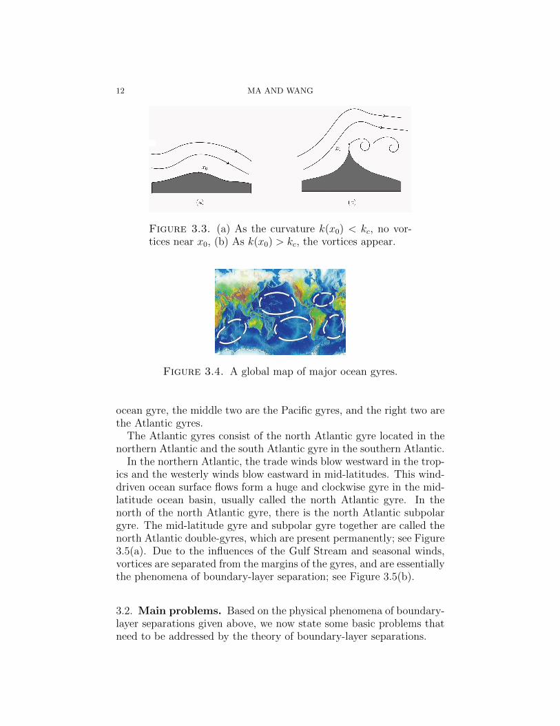
2). Vortex flows near a boundary tip point. At a tip point on theboundary, a fluid flow generates vortices, as shown in Figure 3.3(b); seealso [12, Section 4.1.4]. Let x0 ∈ ∂Ω be a tip point with curvature k(x0).For a given injection velocity u0, there is a critical curvature kc suchthat if k(x0) < kc, there is no vortices forming near x0 for the boundary-layer flow shown in Figure 3.3(a), and if k(x0) > kc (k(x0) = ∞ at acusp point), the vortices appear near x0; see Figure 3.3(b).

3). Wind-driven Atlantic gyres. The oceanic gyres are typical largestructure of large-scale ocean surface circulations. Figure 3.4 providesthe map of the five major oceanic gyres, where the left one is the Indian

12 MA AND WANG

Figure 3.3. (a) As the curvature k(x0) < kc, no vor-tices near x0, (b) As k(x0) > kc, the vortices appear.

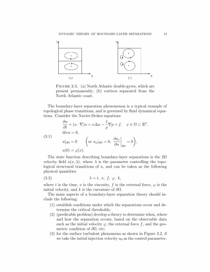
Figure 3.4. A global map of major ocean gyres.

ocean gyre, the middle two are the Pacific gyres, and the right two arethe Atlantic gyres.

The Atlantic gyres consist of the north Atlantic gyre located in thenorthern Atlantic and the south Atlantic gyre in the southern Atlantic.

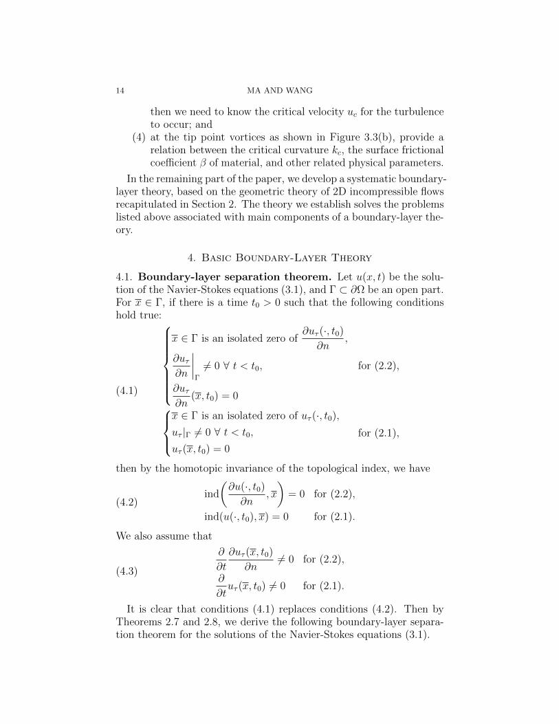
In the northern Atlantic, the trade winds blow westward in the trop-ics and the westerly winds blow eastward in mid-latitudes. This wind-driven ocean surface flows form a huge and clockwise gyre in the mid-latitude ocean basin, usually called the north Atlantic gyre. In thenorth of the north Atlantic gyre, there is the north Atlantic subpolargyre. The mid-latitude gyre and subpolar gyre together are called thenorth Atlantic double-gyres, which are present permanently; see Figure3.5(a). Due to the influences of the Gulf Stream and seasonal winds,vortices are separated from the margins of the gyres, and are essentiallythe phenomena of boundary-layer separation; see Figure 3.5(b).

3.2. Main problems. Based on the physical phenomena of boundary-layer separations given above, we now state some basic problems thatneed to be addressed by the theory of boundary-layer separations.


Figure 3.5. (a) North Atlantic double-gyres, which arepresent permanently; (b) vortices separated from theNorth Atlantic coast.

The boundary-layer separation phenomenon is a typical example oftopological phase transitions, and is governed by fluid dynamical equa-tions. Consider the Navier-Stokes equations

(3.1)

∂u

∂t+ (u · ∇)u = ν∆u− 1

ρ∇p+ f, x ∈ Ω ⊂ R2,

divu = 0,

u|∂Ω = 0

(or un|∂Ω = 0,

∂uτ∂n

∣∣∣∣∂Ω

= 0

),

u(0) = ϕ(x).

The state function describing boundary-layer separations is the 2Dvelocity field u(x, λ), where λ is the parameter controlling the topo-logical structural transitions of u, and can be taken as the followingphysical quantities

(3.2) λ = t, ν, f, ϕ, k,

where t is the time, ν is the viscosity, f is the external force, ϕ is theinitial velocity, and k is the curvature of ∂Ω.

The main aspects of a boundary-layer separation theory should in-clude the following:

(1) establish conditions under which the separations occur and de-termine the critical thresholds;

(2) (predicable problem) develop a theory to determine when, whereand how the separation occurs, based on the observable datasuch as the initial velocity ϕ, the external force f , and the geo-metric condition of ∂Ω, etc;

(3) for the surface turbulent phenomena as shown in Figure 3.2, ifwe take the initial injection velocity u0 as the control parameter,

14 MA AND WANG

then we need to know the critical velocity uc for the turbulenceto occur; and

(4) at the tip point vortices as shown in Figure 3.3(b), provide arelation between the critical curvature kc, the surface frictionalcoefficient β of material, and other related physical parameters.

In the remaining part of the paper, we develop a systematic boundary-layer theory, based on the geometric theory of 2D incompressible flowsrecapitulated in Section 2. The theory we establish solves the problemslisted above associated with main components of a boundary-layer the-ory.

4. Basic Boundary-Layer Theory

4.1. Boundary-layer separation theorem. Let u(x, t) be the solu-tion of the Navier-Stokes equations (3.1), and Γ ⊂ ∂Ω be an open part.For x ∈ Γ, if there is a time t0 > 0 such that the following conditionshold true:

(4.1)

x ∈ Γ is an isolated zero of∂uτ (·, t0)

∂n,

∂uτ∂n

∣∣∣∣Γ

6= 0 ∀ t < t0,

∂uτ∂n

(x, t0) = 0

for (2.2),

x ∈ Γ is an isolated zero of uτ (·, t0),

uτ |Γ 6= 0 ∀ t < t0,

uτ (x, t0) = 0

for (2.1),

then by the homotopic invariance of the topological index, we have

(4.2)ind

(∂u(·, t0)

∂n, x

)= 0 for (2.2),

ind(u(·, t0), x) = 0 for (2.1).

We also assume that

(4.3)

∂

∂t

∂uτ (x, t0)

∂n6= 0 for (2.2),

∂

∂tuτ (x, t0) 6= 0 for (2.1).

It is clear that conditions (4.1) replaces conditions (4.2). Then byTheorems 2.7 and 2.8, we derive the following boundary-layer separa-tion theorem for the solutions of the Navier-Stokes equations (3.1).


Theorem 4.1 (Boundary-layer separation). Let u(x, t) be the solutionof the Navier-Stokes equations (3.1). If u(x, t) satisfies (4.1) and (4.3),then u has a boundary-layer separation at (x, t0).

Remark 4.2. Let X = Br0(Ω,R2) or Br(Ω,R2). Mathematically, con-

ditions (4.3) are generic. Namely, there is an open and dense setU ⊂ X × L2(Ω,R2), such that for any (ϕ, f) ∈ U the solution u(x, t)of (3.1) satisfies (4.3). Hence conditions (4.3) are a physically soundcondition. Moreover, in Theorem 4.1, the conditions (4.3) can also bereplaced by

∂uτ∂n

(x, t) or uτ (x, t)

> 0 for t < t0 (or t > t0),

= 0 for t = t0,

< 0 for t > t0 (or t < t0).

4.2. Separation equations for the rigid boundary condition.To verify the condition (4.1), it is very useful to transform the Navier-Stokes equations (3.1) into the separation equation introduced in thisand next subsections.

1). Separation equation in (τ, n)−representation. In [5], we provedthat the Navier-Stokes equations (3.1) lead to the following boundary-layer separation equation of (3.1) under the rigid boundary condition:

(4.4)∂uτ (x, t)

∂n=∂ϕτ∂n

+

∫ t

0

[ν∇×∆u+ kν∆u · τ +∇× f + kfτ ]dt,

where n, τ are the unit normal and tangent vectors on ∂Ω, k is thecurvature of ∂Ω at x ∈ ∂Ω, and

(4.5) ∇× v =∂vτ∂n− ∂vn

∂τ.

2). Separation equation in (x1, x2)−representation. Consider an or-thogonal coordinate system (x1, x2), the equivalent separation equationof the Navier-Stokes equations was derived in [14]:

(4.6)∂uτ (x, t)

∂n= −∇× ϕ−

∫ t

0

[ν∇×∆u+∇× f ]dt, x ∈ ∂Ω,

where ∇× v = ∂v2/∂x1 − ∂v1/∂x2 for v = (v1, v2).

Remark 4.3. Although the curvature k of ∂Ω doesn’t appear in theseparation equation (4.6), the curvature of ∂Ω is hidden in ∇ × ∆uand ∇ × f , i.e. in the curl of ∆u and f in the orthogonal coordinatesystem.

16 MA AND WANG

4.3. Separation equation for the free boundary condition. Con-sider the Navier-Stokes equations with the free boundary condition:

∂u

∂t+ (u · ∇)u = ν∆u− 1

ρ∇p+ f,(4.7)

divu = 0,(4.8) un = 0,∂uτ∂n

= 0 on ∂Ω,

u(x, 0) = ϕ(x).(4.9)

To deduce the separation equation of (4.7)–(4.9), we recall that forany external f ∈ L2(Ω,R2), as a vector field we know that f can beuniquely decomposed as

f = F +∇φ, divF = 0, and Fn = 0 on ∂Ω.(4.10)

Also, (u · ∇)u is decomposed as

(4.11)(u · ∇)u = g(u) +∇Φ(u),

divg(u) = 0, gn|∂Ω = 0.

Then in the following we shall prove that the separation equation of(4.7)–(4.9) is written in the following form

(4.12) uτ (x, t) = ϕτ (x) +

∫ t

0

[ν

(∂2uτ∂τ 2

+∂2uτ∂n2

)− gτ (u) + Fτ

]dt,

where F and g are as in (4.10) and (4.11).

Remark 4.4. If the portion of the boundary Γ ∈ ∂Ω is flat:

(4.13) Γ = (x1, x2) ∈ ∂Ω | − δ < x1 < δ, x2 = 0,and the velocity gradient ∂u1/∂x1 is small on Γ, then the equation(4.12) can be approximatively written as

(4.14)

u1(x, t) = ϕ1 +

∫ t

0

[ν∆u1 + F1 − A]dt, x = (x1, 0),

A = u1∂u1

∂x1

∣∣∣∣x=0

,

where u1, ϕ1, and F1 are the x1−components of u, ϕ and F .

We are now in position to verify (4.12). By (4.8) and (4.9), we inducefrom the free boundary condition that

4u · n|∂Ω = 0,

and consequentlydiv(∆u) = 0.


Hence, by (4.10) and (4.11), equation (4.7) can be decomposed as

(4.15)

∂u

∂t= ν∆u− g(u) + F,

1

ρp = φ− Φ(u).

Then, we derive from the first equation of (4.15) that

uτ = ϕτ +

∫ t

0

[ν∆uτ − gτ (u) + Fτ ]dt,

which is the equation (4.12).We now verify (4.14). By (4.9), it is clear that

(4.16) (u · ∇)u · τ = u1∂u1

∂x1

on Γ.

By (4.11), in the divergence-free part g = (g1, g2) of (u · ∇)u, g1|x=0

represents the leading order of g1. Hence the Taylor expression of g1

on Γ is given by

g1(x1) = g1(0) + x1f(x1), f1 = g′(0) +1

2g′′1(0)x1 + o(x1).

Since ∂u1/∂x1 is small on Γ, by (4.11) and (4.16) we have

g1(0) x1f(x1) for (x1, 0) ∈ Γ.

Hence, we get that

g1(0) = u1∂u1

∂x1

∣∣∣∣x=0

' gτ (x) on Γ.

Replacing gτ in (4.12) by g1(0), we obtain (4.14).We note that the separation equation (4.14) is more useful than

(4.12) in dealing with fluid boundary-layer separations.

5. Predicable Conditions and Critical Thresholds

5.1. Predicable condition. Predicable problem for boundary-layerseparations of 2D fluid flows governed by Navier-Stokes equations isan important topic in both classical and geophysical fluid dynamics.It mainly concerns when, where, and how a boundary-layer separationwill occur. In particular, we need to know the conditions for the sep-aration to appear in terms of the initial values and the external forcesthat are observable. Based on the basic theory introduced in the lastsection, we now address this problem.

1). Predicable condition of flows with Dirichlet boundary conditionon a flate boundary. When the separation occurs on a flat portion Γ of

18 MA AND WANG

∂Ω, a predicable condition was given in [3]. For the sake of complete-ness, we introduce it in the following.

Let Γ ⊂ ∂Ω be as in (4.13), and x2 > 0 be the interior of Ω. By

ϕ|∂Ω = 0, divϕ = 0,

near Γ, the initial value ϕ = (ϕ1, ϕ2) can be expressed as

(5.1)

ϕ1 = x2ϕ11(x1) + x22ϕ12(x1) + x3

2ϕ13(x1) + o(x32),

ϕ2 = x22ϕ21(x1) + o(x3

2),

ϕ21 = −1

2ϕ′11.

The first-order Taylor expression of the external force f on x2 nearΓ is given by

(5.2)f1 = f11(x1) + x2f12(x1) + o(x2),

f2 = f21(x1) + x2f22(x1) + o(x2).

If the following condition holds true

(5.3) 0 < minΓ

−ϕ11

2νϕ′′11 + 6νϕ13 + f12 − f ′21

1,

then there are t0 > 0 and x0 ∈ Γ such that the solution u of (3.1)has a boundary layer separation at (x0, t0), where ν is the viscosity,ϕ11, ϕ13, f12, f21 are as in (5.1) and (5.2). In addition, t0 and x0 =(x0

1, 0) approximately satisfy

(5.4) t0 = g(x0), and g(x0) = minΓg(x),

where

g =−ϕ11

2νϕ′′11 + 6νϕ13 + f12 − f ′21

.

The condition (5.3), expressed in terms of the initial value ϕ and theexternal force f , provides a criterion for a boundary-layer separationto occur at (x0, t0), and the relations in (5.4) give the time t0 and theposition x0 where the separation occurs.

The proof (5.3) is based on Theorem 4.1 by applying the separationequation (4.4). In fact, on Γ (4.4) can be written as

(5.5)∂u1(x, t)

∂x2

=∂ϕ1

∂x2

+

∫ t

0

[ν∂∆u1

∂x2

− ν ∂∆u2

∂x1

+∂f1

∂x2

− ∂f2

∂x1

]dt.

Take the first-order expression of u on t as

u = ϕ+ tu′(x, t),


and insert it in the right side of (5.5). By (5.1) and (5.2), we obtainthat

∂u1

∂x2

= ϕ11 + t[ν(ϕ′′11 + 6ϕ13 − 2ϕ′21) + f12 − f ′21] + o(t).

Note that ϕ21 = −12ϕ′′11. Then we have

(5.6)∂u1

∂x2

= ϕ11 + t[ν(2ϕ′′11 + 6ϕ13) + f12 − f ′21] + o(t).

Then, under the condition (5.3), we deduce that there are x0 ∈ Γ andt0 > 0 sufficiently small such that

∂uτ∂n

(t, x0)

6= 0 for 0 ≤ t < t0,

= 0 for t = t0.

∂

∂t

∂uτ∂n

∣∣∣∣(t0,x0)

6= 0.

Conclusions of (5.3) and (5.4) follow then from Theorem 4.1.

2). Predicable condition for flows with Dirichlet boundary conditionon a curved boundary. On a curved boundary, a predicable condi-tion for boundary-layer separations can be derived from the separationequations (4.4) and (4.6) respectively, also based on Theorem 4.1.

Let Γ ⊂ ∂Ω be an open and curved portion of the boundary. By(4.4), we can derive the following predicable condition:

(5.7) 0 < minΓ

−∂ϕτ

∂n

ν(∇×∆ϕ+ k∆ϕ · τ) +∇× f + kfτ 1,

where k = k(x) is the curvature of ∂Ω at x ∈ Γ, and ∇ × v is as in(4.5) for the vector field v.

The other predicable condition in the orthogonal coordinate (x1, x2)can be derived from (4.6) as follows (see [14]),

(5.8) 0 < minΓ

∂ϕ2

∂x1− ∂ϕ1

∂x2

ν

(∂∆ϕ1

∂x2− ∂∆ϕ2

∂x1

)+ ∂f1

∂x2− ∂f2

∂x1

1.

3). Predicable conditions of free boundary condition. By the sep-aration equations (4.12) and (4.14), based on Theorem 4.1, we canalso derive predicable conditions for fluid flows with the free boundarycondition.

If Γ ⊂ ∂Ω is a flat portion of the boundary, as given by (4.13), wehave the following criterion to determine a boundary-layer separation

20 MA AND WANG

to occur on Γ:

(5.9) 0 < minΓ

−ϕ1

ν∆ϕ1 + F1 − ϕ1∂ϕ1

∂x1

∣∣x=0

1,

where ϕ1 and F1 are the x1−components of ϕ and F , and F is as in(4.10). If Γ ⊂ ∂Ω is curved, then by (4.12) we deduce the followingpredicable condition:

(5.10) 0 < minΓ

−ϕτ

ν

(∂2ϕτ

∂τ2+ ∂2ϕτ

∂n2

)+ Fτ − gτ (ϕ)

1,

where g is as in (4.11).The five criteria (5.3) and (5.7)–(5.10) for boundary-layer separations

are very useful in wide range of applications.

Remark 5.1. With conditions (5.3) and (5.7)–(5.10), the critical timet0 might appear to be very small; see for example (5.4). However, thismisperception is related to scaling. For a large scale fluid motion, theunderlying dimensions are large, and the time t0 is not small in realapplications.

5.2. Critical curvature of boundary tip point. To discuss vorticesseparated from a boundary tip point we need to use the separationequation (4.4). Let t0 be the elapsed time between the instant whena vortex separated from the tip point disappears and the time when anew one forms. The elapsed time t0 is called the relaxation time forthe tip point separation.

Let x0 ∈ ∂Ω be a boundary tip point with curvature k. Take k asthe control parameter. Then, equation (4.4) becomes

∂uτ (k)

∂n=∂ϕτ (x0)

∂n+

(∂fτ (x0)

∂n− ∂fn(x0)

∂τ+ kfτ (x0)

)t0(5.11)

+

∫ t0

0

ν

[∂(∆u · τ)

∂n− ∂(∆u · n)

∂τ+ k∆u · τ

]x0

dt.

Here, the initial injection flow ϕ(x) is taken parallel to the tangentvector τ at x0, i.e. ϕ represents a parallel gradient flow as

ϕ = (ax2, 0) near x0 ∈ ∂Ω,(5.12)

where the coordinate (x1, x2) is taken so that the x1−axis is in thetangent τ−direction, x2−axis is in the normal n−direction, and x0 isthe origin of this coordinate system; see Figure 5.1. By the definitionof the relaxation time, it is known that t0 is very small. Hence we have

u(x, t) ' ϕ ∀ 0 ≤ t < t0 near x0 ∈ ∂Ω.


Figure 5.1. A schematic diagram of parallel gradientflow near a boundary tip point x0, the shadow part is adead angle where fluid velocity u = 0.

By (5.12), this implies that∫ t0

0

[∂(∆u · τ)

∂n− ∂(∆u · n)

∂τ+ k∆u · τ

]x0

dt ' 0,

and (5.11) can be approximatively written as

(5.13)∂uτ (k)

∂n= a+ kfτ t0 +

(∂fτ∂n− ∂fn

∂τ

)t0.

Because f is the resistance force generated by the friction at x0, it isreversely parallel to ϕ, and we have

∂fn∂τ

= 0,∂fτ∂n' 0.

Thus, (5.13) becomes

(5.14)∂uτ (k)

∂n= a+ kfτ t0 (a > 0, fτ < 0).

For the control parameter k (instead of t), it follows from (5.14) that

(5.15)

∂uτ (k)

∂n

< 0 for k < kc,

= 0 for k = kc,

∂

∂k

∂uτ (kc)

∂n= fτ t0 6= 0,

where kc is the critical curvature, given by

(5.16) kc =a

|fτ |t0.

22 MA AND WANG

Namely, by the boundary-layer separation theorem, Theorem 4.1, un-der the conditions (5.15), the critical curvature kc in (5.16) is the criticalthreshold where vortices begin to form.

Physically, a = |∇ϕ(x0)| is the strength of the injection velocity,which is proportional to the viscosity ν:

a = γν (γ is the coefficient).

The frictional force fτ is proportional to the smoothness of the materialsurface, denoted by κ:

fτ = θκ,

where θ is the proportional coefficient. Therefore, the critical curvaturekc in (5.16) is

(5.17) kc =αν

κt0,

where α = γ/θ is the proportional coefficient.Formula (5.17) shows that the vortices are easier to form if the viscos-

ity of fluid is relatively small, and the surface of the material is rougher(i.e. κ is relatively large). This conforms to the physical reality.

5.3. Critical velocity of surface turbulence. For a boundary flow,when the injection velocity u0 is smaller than a critical threshold uc, itis a parallel shear flow, and when u0 > uc, surface turbulence occurs.The threshold uc is defined as

(5.18) uc = the critical velocity of boundary-layer separation.

Based on this definition, to obtain the critical threshold uc of surfaceturbulence, we only need to consider the critical injection velocity u0

at which the boundary-layer separation occurs. We use the separationequation (4.14) for the free boundary condition to study this problem.

Let t0 > 0 be the relaxation time when the first vortex appears asthe injection velocity u0 arrives at uc, so that t0 > 0 is small. Hence,(4.14) can be approximatively written in the form

(5.19) uτ = ϕτ +

[Fτ + ν

(∂2ϕτ∂τ 2

+∂2ϕτ∂n2

)− ϕτ

∂ϕτ∂τ

∣∣∣∣x=0

]t0,

where Fτ represents the tangent damping resistance, and Γ ⊂ ∂Ω is

(5.20) Γ = (x1, 0) | 0 < x1 < L.

Let u0 be the injection velocity. Take u0 as the control parameter, and

(5.21) ϕτ = u0 − β1x1 + β2x21 (β1 > β2L),


where β1, β2 > 0 are two small parameters, depending on the viscosityν of the fluid and the surface physical property of Γ. By the physicallaw of the damping force,

(5.22) Fτ = −γuk0 (k > 1, γ > 0).

Inserting (5.21) and (5.22), we deduce that

uτ = u0 − β1x1 + β2x21 − (γuk0 − 2β2ν − β1u0)t0.

Because β1x1 and β2x21 are relatively small with respect to u0, and ν is

very small, uτ can be expressed as

uτ = (1 + β1t0)u0 − γuk0t0.Let uτ = 0. Then we obtain the following form of uc:

(5.23) uc =

(1

γt0+β1

γ

)1/(k−1)

(k > 1),

where γ is the damping coefficient, depending on the surface property ofΓ, and β1 is as in (5.21) which is an increasing function of the viscosityν. Let β1 = β0ν. Then (5.23) is rewritten as

(5.24) uc =

[1

γ

(1

t0+ β0ν

)]1/(k−1)

.

Remark 5.2. For the surface turbulent problem, the length L in (5.20)cannot be too large because the velocity decay formula (5.21) holds trueonly for L not large. In fact, the physical phenomena show that surfacefluid turbulence can occur only for L being relative small.

6. Boundary-Layer Separation of Ocean Circulations

The atmospheric and oceanic flows exhibit recurrent large-scale pat-terns. The formation of these patterns are important topological phasetransition problem. The main objective of this section is to study themechanism for the formation of the subpolar gyre and the vorticesseparated from the western boundary of the Atlantic ocean.

6.1. Vortices separated from the boundary. Let Γ ⊂ ∂Ω be a flatportion of the coast, denoted by

(6.1) Γ = (x1, 0) | − δ < x1 < δand x2 > 0 represents the sea area. Let ϕ = (ϕ1, ϕ2) represent theoceanic flow, expressed as

(6.2) ϕ1 =x2u0

2δ + x1

, ϕ2 =x2

2u0

2(2δ + x1)2

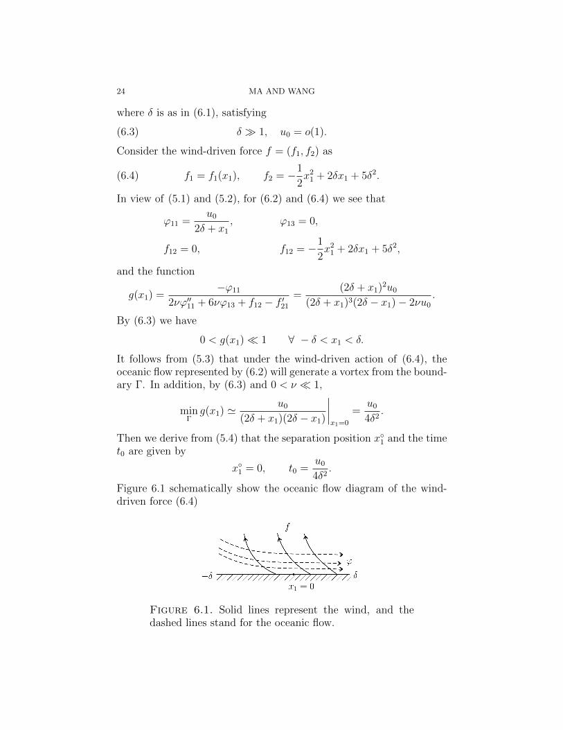
24 MA AND WANG

where δ is as in (6.1), satisfying

(6.3) δ 1, u0 = o(1).

Consider the wind-driven force f = (f1, f2) as

(6.4) f1 = f1(x1), f2 = −1

2x2

1 + 2δx1 + 5δ2.

In view of (5.1) and (5.2), for (6.2) and (6.4) we see that

ϕ11 =u0

2δ + x1

, ϕ13 = 0,

f12 = 0, f12 = −1

2x2

1 + 2δx1 + 5δ2,

and the function

g(x1) =−ϕ11

2νϕ′′11 + 6νϕ13 + f12 − f ′21

=(2δ + x1)2u0

(2δ + x1)3(2δ − x1)− 2νu0

.

By (6.3) we have

0 < g(x1) 1 ∀ − δ < x1 < δ.

It follows from (5.3) that under the wind-driven action of (6.4), theoceanic flow represented by (6.2) will generate a vortex from the bound-ary Γ. In addition, by (6.3) and 0 < ν 1,

minΓg(x1) ' u0

(2δ + x1)(2δ − x1)

∣∣∣∣x1=0

=u0

4δ2.

Then we derive from (5.4) that the separation position x1 and the timet0 are given by

x1 = 0, t0 =u0

4δ2.

Figure 6.1 schematically show the oceanic flow diagram of the wind-driven force (6.4)

Figure 6.1. Solid lines represent the wind, and thedashed lines stand for the oceanic flow.


6.2. Wind-driven north Atlantic gyres. In Section 3.1 we intro-duced the north Atlantic gyres, where a double gyres (as shown in Fig-ure 3.5(a)) is permanent, and some small vortices (as shown in Figure3.5(b)) is seasonal. In this section we discuss the wind-driven vorticesby applying the boundary-layer separation theory.

The dynamical equations governing the wind-driven north Atlanticcirculations are the Navier-Stokes equations with free boundary condi-tion, given by

(6.5)

∂u

∂t+ (u · ∇)u = ν∆u− βy~k × u− 1

ρ∇p+ f, (x, y) ∈ Ω,

divu = 0,

un|∂Ω = 0,∂uτ∂n

∣∣∣∣∂Ω

= 0,

u(0) = ϕ,

where the domain Ω represents the north Atlantic region, approxima-tively in a rectangular region, as

Ω = (0, L)× (−L,L),

with coordinate (x, y), and the x−axis points eastward, the y−axis isnorthward, y = 0 represents the mid-latitude. The term representingthe Coriolis force in (6.5) is

−βy~k × u = −βy(−u2, u1),

where βy is the first-order approximation parameter of the Coriolisforce. The wind-driven force f can be expressed as

(6.6) f = F + F ,where F is the constant force driving the permanent double gyre asshown in Figure 3.5 (a), and F represents the force by seasonal winds.For convenience, F is written in the divergence free part, by (4.12) and(4.14), which dictates the boundary-layer separation:

(6.7) F = λ(F1,F2), with F2(0, y) > 0 for y < L,

where λ is the strength, divF = 0, and F · n|∂Ω = 0.The initial field ϕ represents the north Atlantic double gyre, which

satisfies the stationary equation of (6.5):

(6.8)ν∆ϕ− βy~k × ϕ− (ϕ · ∇)ϕ− 1

ρ∇p+ F = 0,

divϕ = 0,

with the free boundary condition, where F is as in (6.6).

26 MA AND WANG

To use the separation equation (4.14), we take

Γ = (0, y) ∈ ∂Ω | 0 < y < L.Since un|∂Ω = 0, we have

(~k × u) · τ |∂Ω = 0.

Hence, in view of (6.5)–(6.8), the equation (4.14) can be written as

(6.9) u2(y, t) = ϕ2(y) +

∫ t

0

[ν∆u2 − u2

∂u2

∂y

∣∣∣∣y=0

+ f2

]dt.

Let u be denoted by

(6.10) u = ϕ+ v with v|t=0 = 0.

Putting u2 of (6.10) in the right-side of (6.9), by (6.6)–(6.8), we obtainthat

(6.11) u2(y, t) = ϕ2(y) +

∫ t

0

[ν∆u2 − ϕ2

∂v2

∂y− v2

∂ϕ2

∂y− λF2

]dt.

for 0 < y < L.Fixing t0 > 0 small, then by v(y, 0) = 0 and (6.7), the equation

(6.11) can be approximatively expressed in the form

(6.12) u2(y, t0) = ϕ2(y) + λt0F2(y).

By (6.8), in the region of 0 < y < L, the field ϕ describes the northAtlantic subpolar gyre, i.e. the northern counter-clockwise gyre inFigure 3.5(a). Hence, we have

(6.13)ϕ2(y) < 0 for 0 < y < L,

ϕ2(0) = ϕ2(L) = 0.

In addition, by (6.7) and F · n|∂Ω = 0, for the rectangular Ω we have

(6.14)F2(y) > 0, for 0 < y < L,

F2(L) = 0.

It is clear that ϕ2 6= F2. Hence it follows from (6.12)–(6.14) that thereare λc > 0 and an isolated point y0 ∈ (0, L) such athat

(6.15) u2(y0, λ)

< 0 for λ < λc,

= 0 for λ = λc,

> 0 for λ > λc.

By Theorem 4.1 or Remark 4.2, we infer from (6.15) that the solutionu of (6.1) has a boundary-layer separation at (0, y0) ∈ Γ for λ > λc.Namely, we have proved the following physical conclusion.


Physical Conclusion 6.1. If the mid-latitude seasonal wind strengthλ exceeds certain threshold λc, vortices near the north Atlantic coastwill form, as shown in Figure 3.5(b). Moreover, the scale (radius) ofthe vortices is an increasing function of λ− λc.

6.3. North Atlantic subpolar gyre. The North Atlantic doublegyres are formed by the northern subpolar gyre and the southern sub-tropical gyre. The subtropical gyre is caused mainly by winds, andthe subpolar gyre is generated by the Gulf stream along the west-ern boundary and the regional topography; see Figure 6.2 in which aschematically topographic diagram of the North Atlantic double gyreis illustrated. Here we shall discuss the mathematical mechanism for

Figure 6.2. A schematically topography diagram ofthe North Atlantic double gyre: the northern subpolarand the southern subtropical gyre.

the subpolar gyre formation by applying the separation equation (4.4);we shall see that the topographical influence of the North Atlantic,i.e. the curvature k(x0) of the tip point x0 in Figure 6.2, plays a veryimportant role for the formation of the subpolar gyre.

In a neighborhood of the point x0, we take the coordinate (x1, x2)with x0 as its origin, the x1−axis in the tangent direction pointingsouthward, and the x2−axis in the normal direction pointing eastward;see Figure 6.3. Take t0 > 0 small, then the separation equation (4.4)at x0 (i.e. x = 0) can be approximatively written as

∂uτ (k)

∂n=∂ϕτ (x0)

∂n+ νt0

[∂(∆ϕ · τ)

∂n− ∂(∆ϕ · n)

∂τ+ k∆ϕ · τ

]x0

(6.16)

+

(∂fτ (x0)

∂n− ∂fn(x0)

∂τ+ kfτ (x0)

)t0,

28 MA AND WANG

Figure 6.3

where k is the curvature of ∂Ω at x0 (x = 0). Because ϕ represents theGulf stream, and ϕ|∂Ω = 0, we have

∂ϕτ (0)

∂n=∂ϕ1(0)

∂x2

< 0 (see Figure 6.2),

∆ϕ · τ |x=0 =∂2ϕ1(0)

∂x22

,

Due to the curvature k 1, if

∂2ϕ1(0)

∂x22

6= 0, f1(0) 6= 0,

then we can ignore the following terms in (6.16)

νt0

(∂(∆ϕ · τ)

∂n− ∂(∆ϕ · n)

∂τ

)and

∂fτ∂n− ∂fn

∂τ.

Then (6.16) becomes

∂uτ (k)

∂n= −

∣∣∣∣∂ϕ1(0)

∂x2

∣∣∣∣+ kt0

[f1(0) + ν

∂2ϕ1(0)

∂x22

].(6.17)

Under the following condition

f1(x0) + ν∂2ϕ1(0)

∂x22

> 0,(6.18)

by (6.17) we deduce that there is a kc > 0 such that

(6.19)∂uτ (k)

∂n

< 0 for k < kc,

= 0 for k = kc,

> 0 for k > kc.

By Theorem 4.1, it follows from (6.19) that if k > kc, then there existsa counter-clockwise gyre in the north of the subtropic gyre. Hence, wehave the following results.


Physical Conclusion 6.2. The condition for the subpolar gyre to ap-pear is that the curvature k of ∂Ω at x0 in Figure 6.2 is sufficientlylarge, and the Gulf stream velocity field ϕ = (ϕ1, ϕ2) and external forc-ing f = (f1, f2) at x0 satisfy the inequality (6.18).

References

[1] M. Ghil, T. Ma, and S. Wang, Structural bifurcation of 2-D incompressibleflows, Indiana Univ. Math. J., 50 (2001), pp. 159–180. Dedicated to ProfessorsCiprian Foias and Roger Temam (Bloomington, IN, 2000).

[2] J. M. Kosterlitz and D. J. Thouless, Ordering, metastability and phasetransitions in two-dimensional systems, Journal of Physics C: Solid StatePhysics, 6 (1973), p. 1181.

[3] H. Luo, Q. Wang, and T. Ma, A predictable condition for boundary layerseparation of 2-d incompressible fluid flows, Nonlinear Anal. Real World Appl.,22 (2015), pp. 336–341.

[4] T. Ma and S. Wang, Boundary layer separation and structural bifurcationfor 2-D incompressible fluid flows, Discrete Contin. Dyn. Syst., 10 (2004),pp. 459–472. Partial differential equations and applications.

[5] , Geometric theory of incompressible flows with applications to fluid dy-namics, vol. 119 of Mathematical Surveys and Monographs, American Math-ematical Society, Providence, RI, 2005.

[6] , Boundary-layer and interior separations in the Taylor-Couette-Poiseuille flow, J. Math. Phys., 50 (2009), pp. 033101, 29.

[7] , Phase Transition Dynamics, Springer-Verlag, xxii, 555pp., 2013.[8] , Topological Phase Transition V: Interior Separation and Cyclone For-

mation Theory, in preparation, (2017).[9] , Topological Phase Transitions I: Quantum Phase Transitions, Hal

preprint: hal-01651908, (2017).[10] , Topological Phase Transitions II: Spiral Structure of Galaxies, Hal

preprint: hal-01671178, (2017).[11] , Topological Phase Transitions III: Solar Surface Eruptions and

Sunspots, Hal preprint: hal-01672381, (2017).[12] H. Oertel, Prandtl-Fuhrer durch die Stromungslehre, Vieweg+Teubner Ver-

lag, 2001.[13] L. Prandtl, in Verhandlungen des dritten internationalen Mathematiker-

Kongresses, Heidelberg, Leipeizig, pp. 484-491, 1904.[14] Q. Wang, H. Luo, and T. Ma, Boundary layer separation of 2-d incompress-

ible dirichlet flows, Discrete Contin. Dyn. Syst. Ser. B, 20 (2015), pp. 675–682.

(Ma) Department of Mathematics, Sichuan University, Chengdu, P.R. China

E-mail address: [email protected]

(Wang) Department of Mathematics, Indiana University, Blooming-ton, IN 47405

E-mail address: [email protected]

topological phase transitions iv: dynamic theory … · topological phase transitions iv: dynamic...

Documents