topicsinsparsemultivariatestatistics ...web.stanford.edu/~hastie/theses/thesis_mazumder.pdfjerry’s...
TRANSCRIPT

TOPICS IN SPARSE MULTIVARIATE STATISTICS
A DISSERTATION
SUBMITTED TO THE DEPARTMENT OF STATISTICS
AND THE COMMITTEE ON GRADUATE STUDIES
OF STANFORD UNIVERSITY
IN PARTIAL FULFILLMENT OF THE REQUIREMENTS
FOR THE DEGREE OF
DOCTOR OF PHILOSOPHY
Rahul Mazumder
August 2012

c© Copyright by Rahul Mazumder 2012
All Rights Reserved
ii

I certify that I have read this dissertation and that, in my opinion, it is fully
adequate in scope and quality as a dissertation for the degree of Doctor of
Philosophy.
(Trevor Hastie) Principal Adviser
I certify that I have read this dissertation and that, in my opinion, it is fully
adequate in scope and quality as a dissertation for the degree of Doctor of
Philosophy.
(Jerome Friedman)
I certify that I have read this dissertation and that, in my opinion, it is fully
adequate in scope and quality as a dissertation for the degree of Doctor of
Philosophy.
(Robert Tibshirani)
Approved for the University Committee on Graduate Studies
iii

Abstract
In this thesis, we visit three topics in modern sparse multivariate analysis that has received
and still continues to receive significant interest in applied statistics in recent years:
• Sparse high dimensional regression
(This work appears in our paper Mazumder et al. (2010).)
• Low-rank matrix completion & collaborative filtering
(This work appears in our paper Mazumder et al. (2011).)
• Sparse undirected gaussian graphical models
(This work appears in our papers Mazumder & Hastie (2012) and Mazumder & Hastie
(2011).)
A main challenge in high dimensional multivariate analysis is in developing scalable and
efficient algorithms for large scale problems that naturally arise in scientific and industrial
applications. This thesis explores the computational challenges that arise in these problems.
We develop and analyze statistically motivated algorithms for various models arising in the
aforementioned areas. This enhances our understanding of algorithms, sheds novel insights
on the statistical problems and leads to computational strategies that appear to outperform
state of the art. A salient feature of this work lies in the exchange of ideas and machinery
across the fields of statistics, machine learning, (convex) optimization and numerical linear
algebra.
iv

Acknowledgements
This thesis would not have been possible without the support of people who stood by me
during my years at Stanford. I would like to convey my sincere thanks to all of them.
Firstly, I would like to thank my adviser, Trevor Hastie, and all the other thesis
committee-members: Emmanuel Candes, Jerome Friedman, Michael Saunders and Robert
Tibshirani for being a part of my committee.
I would like to express my appreciation and deep gratitude to Trevor for being a great
adviser, a great teacher and a wonderful person to work with. I have learned many good
things from him both on the academic and personal front. He has been there to share ideas
and at the same time encourage me to pursue my own. He has been extremely enthusiastic
and supportive throughout my PhD years. My journey in applied statistics and machine
learning would not have been possible without him. A big thanks to the Hasties, specially
Lynda, for the numerous delicious dinners and being great hosts.
I would like to convey my humble thanks to Jerome Friedman, for being a great mentor.
Jerry’s tremendous intellectual energy, enthusiasm, depth of knowledge and deep thinking
have inspired me a lot. I immensely benefited from discussions with him on various topics
related to this thesis — I am indebted to him for his time and patience. I would like to
take this opportunity to express my sincere thanks to Emmanuel Candes, for his advice
and discussions related to various academic topics, especially Convex Optimization and
Matrix Completion. Emmanuel’s enthusiasm, passion and positive energy will have a lasting
impression on me. I greatly value his feedback and suggestions during my presentations at
his group meetings. I would like to convey my regards to Jonathan Taylor. He has always
been there to discuss ideas and talk about different academic topics related or unrelated
to this thesis. Thanks also to Robert Tibshirani, for being a co-author in the matrix
completion work. I greatly acknowledge his support and feedback on various occasions
during the course of the last five years. A big thanks to Naras, for being supportive and a
v

great friend. Finally, I would like to express my appreciation to the all the Stanford faculty
members whom I came across at some point or the other, during my stint as a graduate
student. A big thanks goes to Deepak Agarwal, my mentor at Yahoo! Research (during my
summer internships in 2009 and 2010) for being a great collaborator and friend.
My appreciation goes out to all the members of the Hastie-Tibshirani-Taylor research
group; Emmanuel’s research group and the other students of the Statistics department for
creating an intellectually stimulating environment.
A big thanks to my friends and colleagues at Stanford, specially: Anirban, Arian,
Bhaswar, Brad, Camilor, Dennis, Ewout, Gourab, Jason, Jeremy, Kshitij-da, Leo, Shilin,
Sumit, Victor, Will, Zhen — without whom my stay here would have been nowhere as en-
joyable. A warmly acknowledge the support of some of my close friends from ISI, specially
GP and Saha for being there beside me through my ups and downs. I would also like to
reach out to Debapriya Sengupta from ISI and express my gratitude for encouraging me to
embark on this adventure.
I would like to thank my parents and brother for their endless love and support and
letting me pursue a PhD at Stanford, far away from home. My parents have always stood
by me and encouraged me to pursue my dreams — I dedicate this thesis to them for their
encouragement, sacrifice and unconditional support. A big thanks Lisa, for her love and
support; and for being a wonderful person to be with.
vi

Contents
Abstract iv
Acknowledgements v
1 Introduction 1
I Non-Convex Penalized Sparse Regression 4
2 SparseNet : Non-Convex Coordinate Descent 5
2.1 Introduction . . . . . . . . . . . . . . . . . . . . . . . . . . . . . . . . . . . . 5
2.2 Generalized Thresholding Operators . . . . . . . . . . . . . . . . . . . . . . 10
2.3 SparseNet : coordinate-wise algorithm for constructing the entire regulariza-
tion surface βλ,γ . . . . . . . . . . . . . . . . . . . . . . . . . . . . . . . . . 13
2.4 Properties of families of non-convex penalties . . . . . . . . . . . . . . . . . 15
2.4.1 Effect of multiple minima in univariate criteria . . . . . . . . . . . . 16
2.4.2 Effective df and nesting of shrinkage-thresholds . . . . . . . . . . . . 17
2.4.3 Desirable properties for a family of threshold operators for non-convex
regularization . . . . . . . . . . . . . . . . . . . . . . . . . . . . . . . 19
2.5 Illustration via the MC+ penalty . . . . . . . . . . . . . . . . . . . . . . . . 21
2.5.1 Calibrating MC+ for df . . . . . . . . . . . . . . . . . . . . . . . . . 22
2.6 Convergence Analysis . . . . . . . . . . . . . . . . . . . . . . . . . . . . . . 27
2.7 Simulation Studies . . . . . . . . . . . . . . . . . . . . . . . . . . . . . . . . 28
2.7.1 Discussion of Simulation Results . . . . . . . . . . . . . . . . . . . . 30
2.8 Other methods of optimization . . . . . . . . . . . . . . . . . . . . . . . . . 33
2.8.1 Empirical performance and the role of calibration . . . . . . . . . . . 35
vii

2.A Primary Appendix to Chapter 2 . . . . . . . . . . . . . . . . . . . . . . . . 37
2.A.1 Convergence Analysis for Algorithm 1 . . . . . . . . . . . . . . . . . 37
2.2 Secondary Appendix to Chapter 2 . . . . . . . . . . . . . . . . . . . . . . . 40
2.2.1 Calibration of MC+ and Monotonicity Properties of λS , γλS . . . . 45
2.2.2 Parametric functional form for λS(λ, γ) . . . . . . . . . . . . . . . . 48
2.2.3 Understanding the sub-optimality of LLA through examples . . . . . 51
II Matrix Completion & Collaborative Filtering 56
3 Spectral Regularization Algorithms 57
3.1 Introduction . . . . . . . . . . . . . . . . . . . . . . . . . . . . . . . . . . . . 58
3.2 Context and Related Work . . . . . . . . . . . . . . . . . . . . . . . . . . . 61
3.3 Soft-Impute–an Algorithm for Nuclear Norm Regularization . . . . . . . . 64
3.3.1 Notation . . . . . . . . . . . . . . . . . . . . . . . . . . . . . . . . . . 64
3.3.2 Nuclear Norm Regularization . . . . . . . . . . . . . . . . . . . . . . 64
3.3.3 Algorithm . . . . . . . . . . . . . . . . . . . . . . . . . . . . . . . . . 65
3.4 Convergence Analysis . . . . . . . . . . . . . . . . . . . . . . . . . . . . . . 66
3.4.1 Asymptotic Convergence . . . . . . . . . . . . . . . . . . . . . . . . . 67
3.4.2 Convergence Rate . . . . . . . . . . . . . . . . . . . . . . . . . . . . 70
3.5 Computational Complexity . . . . . . . . . . . . . . . . . . . . . . . . . . . 71
3.6 Generalized Spectral Regularization: From Soft to Hard Thresholding . . . 73
3.7 Post-processing of “Selectors” and Initialization . . . . . . . . . . . . . . . . 77
3.8 Soft-Impute and Maximum-Margin Matrix Factorization . . . . . . . . . . . 78
3.8.1 Proof of Theorem 8 . . . . . . . . . . . . . . . . . . . . . . . . . . . 82
3.9 Numerical Experiments and Comparisons . . . . . . . . . . . . . . . . . . . 83
3.9.1 Observations . . . . . . . . . . . . . . . . . . . . . . . . . . . . . . . 88
3.9.2 Comparison with Fast MMMF . . . . . . . . . . . . . . . . . . . . . 89
3.9.3 Comparison with Nesterov’s Accelerated Gradient Method . . . . . 91
3.9.4 Large Scale Simulations for Soft-Impute . . . . . . . . . . . . . . . 94
3.10 Application to the Netflix Data Set . . . . . . . . . . . . . . . . . . . . . . . 94
3.A Appendix to Chapter 3 . . . . . . . . . . . . . . . . . . . . . . . . . . . . . . 96
3.A.1 Proof of Lemma 6 . . . . . . . . . . . . . . . . . . . . . . . . . . . . 97
3.A.2 Proof of Lemma 8 . . . . . . . . . . . . . . . . . . . . . . . . . . . . 99
viii
3.A.3 Proof of Lemma 9 . . . . . . . . . . . . . . . . . . . . . . . . . . . . 102
3.A.4 Proof of Lemma 10 . . . . . . . . . . . . . . . . . . . . . . . . . . . . 103
3.A.5 Proof of Lemma 11 . . . . . . . . . . . . . . . . . . . . . . . . . . . . 105
3.A.6 Proof of Theorem 7 . . . . . . . . . . . . . . . . . . . . . . . . . . . 107
III Covariance Selection & Graphical Lasso : New Insights & Alter-
natives 110
4 Exact Covariance Thresholding for glasso 112
4.1 Introduction . . . . . . . . . . . . . . . . . . . . . . . . . . . . . . . . . . . . 113
4.1.1 Notations and preliminaries . . . . . . . . . . . . . . . . . . . . . . . 114
4.2 Methodology: Exact Thresholding of the Covariance Graph . . . . . . . . . 115
4.2.1 Related Work . . . . . . . . . . . . . . . . . . . . . . . . . . . . . . . 119
4.3 Computational Complexity . . . . . . . . . . . . . . . . . . . . . . . . . . . 120
4.4 Numerical examples . . . . . . . . . . . . . . . . . . . . . . . . . . . . . . . 121
4.4.1 Synthetic examples . . . . . . . . . . . . . . . . . . . . . . . . . . . . 121
4.4.2 Micro-array Data Examples . . . . . . . . . . . . . . . . . . . . . . . 123
4.5 Conclusions . . . . . . . . . . . . . . . . . . . . . . . . . . . . . . . . . . . . 126
4.A Appendix to Chapter 4 . . . . . . . . . . . . . . . . . . . . . . . . . . . . . . 127
4.A.1 Proof of Theorem 9 . . . . . . . . . . . . . . . . . . . . . . . . . . . 127
4.A.2 Proof of Theorem 10 . . . . . . . . . . . . . . . . . . . . . . . . . . . 130
5 glasso New Insights and Alternatives 131
5.1 Introduction . . . . . . . . . . . . . . . . . . . . . . . . . . . . . . . . . . . . 132
5.2 Review of the glasso algorithm. . . . . . . . . . . . . . . . . . . . . . . . . 133
5.3 A Corrected glasso block coordinate-descent algorithm . . . . . . . . . . . 137
5.4 What is glasso actually solving? . . . . . . . . . . . . . . . . . . . . . . . . 138
5.4.1 Dual of the ℓ1 regularized log-likelihood . . . . . . . . . . . . . . . . 139
5.5 A New Algorithm — dp-glasso . . . . . . . . . . . . . . . . . . . . . . . . 143
5.6 Computational Costs in Solving the Block QPs . . . . . . . . . . . . . . . . 145
5.7 glasso: Positive definiteness, Sparsity and Exact Inversion . . . . . . . . . 147
5.8 Warm Starts and Path-seeking Strategies . . . . . . . . . . . . . . . . . . . 148
5.9 Experimental Results & Timing Comparisons . . . . . . . . . . . . . . . . . 152
ix

5.9.1 Synthetic Experiments . . . . . . . . . . . . . . . . . . . . . . . . . . 152
5.9.2 Micro-array Example . . . . . . . . . . . . . . . . . . . . . . . . . . . 160
5.10 Conclusions . . . . . . . . . . . . . . . . . . . . . . . . . . . . . . . . . . . . 161
5.A Appendix to Chapter 5 . . . . . . . . . . . . . . . . . . . . . . . . . . . . . . 161
5.A.1 Examples: Non-Convergence of glasso with warm-starts . . . . . . 162
5.B Further Experiments and Numerical Studies . . . . . . . . . . . . . . . . . . 163
Bibliography 165
x

List of Tables
2.1 Table showing standardized prediction error (SPE), percentage of non-zeros and
zero-one error in the recovered model via SparseNet, for different problem instances.
Values within parenthesis (in subscripts) denote the standard errors, and the true
number of non-zero coefficients in the model are in square braces. Results are aver-
aged over 25 runs. . . . . . . . . . . . . . . . . . . . . . . . . . . . . . . . . . 31
3.1 Performances of Soft-Impute andMMMF for different problem instances, in terms
of test error (with standard errors in parentheses), training error and times for
learning the models. Soft-Impute,“rank” denotes the rank of the recovered matrix,
at the optimally chosen value of λ. For the MMMF, “rank” indicates the value of
r′ in Um×r′, Vn×r′ . Results are averaged over 50 simulations. . . . . . . . . . . . 90
3.2 Four different examples used for timing comparisons of Soft-Impute and (acceler-
ated) Nesterov. In all cases the SNR= 10. . . . . . . . . . . . . . . . . . . . . 92
3.3 Performance of Soft-Impute on different problem instances. All models are gen-
erated with SNR=10 and underlying rank=5. Recovered rank is the rank of the
solution matrix Z at the value of λ used in (3.10). Those with stars reached the
“maximum rank” threshold, and option in our algorithm. Convergence criterion is
taken as “fraction of improvement of objective value” less than 10−4 or a maximum
of 15 iterations for the last four examples. All implementations are done in MAT-
LAB including the MATLAB implementation of PROPACK on a Intel Xeon Linux
3GHz processor. . . . . . . . . . . . . . . . . . . . . . . . . . . . . . . . . . . 95
3.4 Results of applying Soft-Impute to the Netflix data. λ0 = ||PΩ(X)||2; see Sec-
tion 3.9.4. The computations were done on a Intel Xeon Linux 3GHz processor;
timings are reported based on MATLAB implementations of PROPACK and our
algorithm. RMSE is root-mean squared error, as defined in the text. . . . . . . . 96
xi

4.1 Table showing (a) the times in seconds with screening, (b) without screening i.e. on
the whole matrix and (c) the ratio (b)/(a) – ‘Speedup factor’ for algorithms glasso
and smacs. Algorithms with screening are operated serially—the times reflect the
total time summed across all blocks. The column ‘graph partition’ lists the time for
computing the connected components of the thresholded sample covariance graph.
Since λII > λI , the former gives sparser models. ‘*’ denotes the algorithm did not
converge within 1000 iterations. ‘-’ refers to cases where the respective algorithms
failed to converge within 2 hours. . . . . . . . . . . . . . . . . . . . . . . . . . 124
5.1 Table showing the performances of the four algorithms glasso (Dual-Warm/Cold)
and dp-glasso (Primal-Warm/Cold) for the covariance model Type-1. We present
the times (in seconds) required to compute a path of solutions to (5.1) (on a grid of
twenty λ values) for different (n, p) combinations and relative errors (as in (5.40)).
The rightmost column gives the averaged sparsity level across the grid of λ values.
dp-glasso with warm-starts is consistently the winner across all the examples. . . 157
5.2 Table showing comparative timings of the four algorithmic variants of glasso and
dp-glasso for the covariance model in Type-2. This table is similar to Table 5.1,
displaying results for Type-1. dp-glasso with warm-starts consistently outperforms
all its competitors. . . . . . . . . . . . . . . . . . . . . . . . . . . . . . . . . . 159
5.3 Comparisons among algorithms for a microarray dataset with n = 62 and p = 725,
for different tolerance levels (TOL). We took a grid of fifteen λ values, the average
% of zeros along the whole path is 90.8. . . . . . . . . . . . . . . . . . . . . . . 160
xii

List of Figures
2.1 Regularization path for LASSO (left), MC+ (non-convex) penalized least-squares
for γ = 6.6 (centre) and γ = 1+ (right), corresponding to the hard-thresholding
operator (best subset). The true coefficients are shown as horizontal dotted lines.
Here LASSO is sub-optimal for model selection, as it can never recover the true
model. The other two penalized criteria are able to select the correct model (vertical
lines), with the middle one having smoother coefficient profiles than best subset on
the right. . . . . . . . . . . . . . . . . . . . . . . . . . . . . . . . . . . . . . . 8
2.2 Non-Convex penalty families and their corresponding threshold functions. All are
shown with λ = 1 and different values for γ. . . . . . . . . . . . . . . . . . . . 12
2.3 The penalized least-squares criterion (2.8) with the log-penalty (2.10) for (γ, λ) =
(500, 0.5) for different values of β. The “*” denotes the global minima of the func-
tions. The “transition” of the minimizers, creates discontinuity in the induced
threshold operators. . . . . . . . . . . . . . . . . . . . . . . . . . . . . . . . . 15
2.4 [Left] The df (solid line) for the (uncalibrated) MC+ threshold operators as a func-
tion of γ, for a fixed λ = 1. The dotted line shows the df after calibration. [Middle]
Family of MC+ threshold functions, for different values of γ, before calibration. All
have shrinkage threshold λS = 1. [Right] Calibrated versions of the same. The
shrinkage threshold of the soft-thresholding operator is λ = 1, but as γ decreases,
λS increases, forming a continuum between soft and hard thresholding. . . . . . 18
2.5 Recalibrated values of λ via λS(γ, λ) for the MC+ penalty. The values of λ at the
top of the plot correspond to the LASSO. As γ decreases, the calibration increases
the shrinkage threshold to achieve a constant univariate df. . . . . . . . . . . . . 26
xiii

2.6 Examples S1 and M1. The three columns of plots represent prediction error, re-
covered sparsity and zero-one loss (all with standard errors over the 25 runs). Plots
show the recalibrated MC+ family for different values of γ (on the log-scale) via
SparseNet, LLA, MLLA, LASSO (las), step-wise (st) and best-subset (bs) (for S1
only) . . . . . . . . . . . . . . . . . . . . . . . . . . . . . . . . . . . . . . . . 29
2.7 Top row: objective function for SparseNet compared to other coordinate-wise vari-
ants — Type (a), (b) and MLLA Type (c) — for a typical example. Plots are shown
for 50 values of γ (some are labeled in the legend) and at each value of γ, 20 values
of λ. Bottom row: relative increase I(γ, λ) in the objective compared to SparseNet,
with the average I reported at the top of each plot. . . . . . . . . . . . . . . . . 35
2.8 Boxplots of I over 24 different examples. In all cases SparseNet shows superior
performance. . . . . . . . . . . . . . . . . . . . . . . . . . . . . . . . . . . . . 36
2.9 Mlla(β) for the univariate log-penalized least squares problem. The starting point
β1 determines which stationary point the LLA sequence will converge to. If the
starting point is on the right side of the phase transition line (vertical dotted line),
then the LLA will converge to a strictly sub-optimal value of the objective function.
In this example, the global minimum of the one-dimensional criterion is at zero. . 53
3.1 Comparison of the parameter space for MMMF (grey and black points), and Soft-
Impute (red squares) for a simple example. Since all MMMF solutions with pa-
rameters above the red squares are identical to the Soft-Impute solutions at the
red squares, all the grey points are redundant. . . . . . . . . . . . . . . . . . . . 80
3.2 Figure showing training/test error profiles for Soft-Impute+, Soft-Impute, Hard-
Impute OptSpace, SVT, MMMF (with full rank 100). Values of test error larger
than one are not shown in the figure. OptSpace is evaluated for ranks ≤ 30. . . . 85
3.3 Soft-Impute+ has the best prediction error, closely followed by Soft-Impute
and MMMF. Both Hard-Impute and OptSpace have poor prediction error apart
from near the true rank. OptSpace is evaluated for a series of ranks ≤ 35. SVT
has poor predictiion error with rank of the solution being > 60. . . . . . . . . . . 86
3.4 With low noise, the performance of Hard-Impute improves and has the best pre-
diction error, followed by OptSpace. SVT did not converge within 1000 iterations,
and the solution seems to be different from the limiting solution of Soft-Impute . 87
xiv

3.5 Timing comparisons of Soft-Impute and (accelerated) Nesterov over a grid of
λ values for examples i–iv. The horizontal axis corresponds to the standardized
nuclear norm, with C = maxλ ‖Zλ‖∗. Results are averaged over 10 simulations. . . 93
4.1 Figure showing the size distribution (in the log-scale) of connected components aris-
ing from the thresholded sample covariance graph for examples (A)-(C). For every
value of λ (vertical axis), the horizontal slice denotes the sizes of the different com-
ponents appearing in the thresholded covariance graph. The colors represent the
number of components in the graph having that specific size. For every figure, the
range of λ values is chosen such that the maximal size of the connected components
do not exceed 1500. . . . . . . . . . . . . . . . . . . . . . . . . . . . . . . . . 127
5.1 [Left panel] The objective values of the primal criterion (5.1) and the dual crite-
rion (5.19) corresponding to the covariance matrixW produced by glasso algorithm
as a function of the iteration index (each column/row update). [Middle Panel] The
successive differences of the primal objective values — the zero crossings indicate
non-monotonicity. [Right Panel] The successive differences in the dual objective
values — there are no zero crossings, indicating that glasso produces a monotone
sequence of dual objective values. . . . . . . . . . . . . . . . . . . . . . . . . . 136
5.2 Figure illustrating some negative properties of glasso using a typical numerical
example. [Left Panel] The precision matrix produced after every row/column update
need not be the exact inverse of the working covariance matrix — the squared
Frobenius norm of the error is being plotted across iterations. [Right Panel] The
estimated precision matrix Θ produced by glasso need not be positive definite
along iterations; plot shows minimal eigen-value. . . . . . . . . . . . . . . . . . . 147
5.3 The timings in seconds for the four different algorithmic versions: glasso (with and
without warm-starts) and dp-glasso (with and without warm-starts) for a grid of
λ values on the log-scale. [Left Panel] Covariance model for Type-1, [Right Panel]
Covariance model for Type-2. The horizontal axis is indexed by the proportion of
zeros in the solution. The vertical dashed lines correspond to the optimal λ values
for which the estimated errors ‖Θλ−Θ‖1 (green) and ‖Θλ−Θ‖F (blue) are minimum.158
xv

5.4 The timings in seconds for the four different algorithmic versions glasso (with and
without warm-starts) and dp-glasso (with and without warm-starts) for a grid of
twenty λ values on the log-scale. The horizontal axis is indexed by the proportion
of zeros in the solution. . . . . . . . . . . . . . . . . . . . . . . . . . . . . . . . 164
xvi

Chapter 1
Introduction
A principal task of modern statistical learning is to make meaningful inference based on
available data which comes in diverse forms from genomic, internet, finance, environmental,
marketing (among other) applications. In the ‘high dimensional’ setting a lot of exciting
research is being conducted in learning sparse, parsimonious and interpretable models via
the ℓ1 penalization (aka LASSO) framework (Tibshirani 2011, for example). A large part
of this is motivated by high-impact real-life applications. The advent of new, complex and
large-scale data-structures from different applications in science and industry requires ex-
tending the scope of existing methods to structured sparse regression, matrix regularization
and covariance estimation. An important and challenging research direction in this context
is in developing statistical models for these tasks, building efficient algorithms for them and
exploring the trade-offs between algorithmic scalability and statistical inference. This thesis
addresses this important theme. What is particularly exciting in this effort is the cross-
fertilization of concepts and tools across the disciplines of statistics and machine learning,
convex optimization (and analysis) and numerical linear algebra.
This thesis covers three topics, based on a series of papers by us; and can be classified
under under the following broad divisions:
1

CHAPTER 1. INTRODUCTION 2
Part I: Non-Convex Penalized Sparse Regression
This chapter develops df calibrated path-approaches to non-convex penalized regres-
sion, significantly improving upon existing algorithms for this task.
Part I of the thesis is based on joint work with Trevor Hastie and Jerome Friedman
and appears in our paper Mazumder et al. (2011);
Part II: Matrix Completion and Collaborative Filtering
This part studies (convex) nuclear-norm relaxations of (non-convex) low-rank con-
straints and exploring the connections with more traditional low-rank matrix fac-
torization based methods. Certain non-convex variants of the rank penalty are also
covered.
Part II of the thesis is based on joint work with Trevor Hastie and Robert Tibshirani
and appears in our paper Mazumder et al. (2010);
Part III: Covariance Selection & Graphical Lasso : New Insights & Alternatives
This part of the thesis is further sub-divided into Chapters‘4 and 5:
• Exact Covariance Thresholding for glasso :
This is about a previously unknown and interesting property of Graphical Lasso
aka glasso which establishes the equivalence between the connected components
of the sparse precision graph and the same of a thresholded version of the sample
covariance matrix. This extends the scope of applications to problems with
number of nodes ranging from tens of thousands to possibly a million (current
technology has trouble in scaling beyond 1-2 K nodes).
This part of the thesis is based on joint work with Trevor Hastie, and appears
in our paper Mazumder & Hastie (2012).
• glasso New Insights and Alternatives:
This chapter highlights some of the properties of the glasso algorithm (Friedman,

CHAPTER 1. INTRODUCTION 3
Hastie & Tibshirani 2007) that appear mysterious and provides explanations to
them. In the process of our analysis, we propose new (and superior) algorithm(s)
on the primal: p-glasso and dp-glasso and justify their usefulness.
This part is based on joint work with Trevor Hastie, and can be found in our
article Mazumder & Hastie (2011).

Part I
Non-Convex Penalized Sparse
Regression
4

Chapter 2
SparseNet : Non-Convex
Coordinate Descent
Abstract: In this chapter we address the problem of sparse selection in linear models. A num-
ber of non-convex penalties have been proposed in the literature for this purpose, along with a
variety of convex-relaxation algorithms for finding good solutions. In this chapter we pursue a
coordinate-descent approach for optimization, and study its convergence properties. We charac-
terize the properties of penalties suitable for this approach, study their corresponding threshold
functions, and describe a df -standardizing reparametrization that assists our pathwise algorithm.
The MC+ penalty (Zhang 2010) is ideally suited to this task, and we use it to demonstrate the
performance of our algorithm.
The content of this chapter is based on joint work with Jerome Friedman and Trevor Hastie;
and the work appears in our paper Mazumder et al. (2011).
2.1 Introduction
Consider the usual linear regression set-up
y = Xβ + ǫ (2.1)
5

CHAPTER 2. SPARSENET: NON-CONVEX COORDINATE DESCENT 6
with n observations and p features X = [x1, . . . ,xp], response y, coefficient vector β and
(stochastic) error ǫ. In many modern statistical applications with p ≫ n, the true β vec-
tor is often sparse, with many redundant predictors having coefficient zero. We would
like to identify the useful predictors and also obtain good estimates of their coefficients.
Identifying a set of relevant features from a list of many thousand is in general combina-
torially hard and statistically troublesome. In this context, convex relaxation techniques
such as the LASSO (Tibshirani 1996, Chen & Donoho 1994) have been effectively used for
simultaneously producing accurate and parsimonious models. The LASSO solves
minβ
12‖y −Xβ‖2 + λ‖β‖1. (2.2)
The ℓ1 penalty shrinks coefficients towards zero, and can also set many coefficients to be
exactly zero. In the context of variable selection, the LASSO is often thought of as a convex
surrogate for best-subset selection:
minβ
12‖y −Xβ‖2 + λ‖β‖0. (2.3)
The ℓ0 penalty ‖β‖0 =∑p
i=1 I(|βi| > 0) penalizes the number of non-zero coefficients in the
model.
The LASSO enjoys attractive statistical properties (Zhao & Yu 2006, Donoho 2006,
Knight & Fu 2000, Meinshausen & Buhlmann 2006). Under certain regularity conditions
on X, it produces models with good prediction accuracy when the underlying model is rea-
sonably sparse. Zhao & Yu (2006) established that the LASSO is model selection consistent:
Pr(A = A0) → 1, where A0 corresponds to the set of nonzero coefficients (active) in the
true model and A those recovered by the LASSO. Typical assumptions limit the pairwise
correlations between the variables.
However, when these regularity conditions are violated, the LASSO can be sub-optimal

CHAPTER 2. SPARSENET: NON-CONVEX COORDINATE DESCENT 7
in model selection (Zhang 2010, Zhang & Huang 2008, Friedman 2008, Zou & Li 2008,
Zou 2006). Since the LASSO both shrinks and selects, it often selects a model which is
overly dense in its effort to relax the penalty on the relevant coefficients. Typically in such
situations greedier methods like subset regression and the non-convex methods we discuss
here achieve sparser models than the LASSO for the same or better prediction accuracy,
and enjoy superior variable-selection properties.
There are computationally attractive algorithms for the LASSO. The piecewise-linear
LASSO coefficient paths can be computed efficiently via the LARS (homotopy) algorithm
(Efron et al. 2004, Osborne et al. 2000). Coordinate-wise optimization algorithms (Friedman
et al. 2009) appear to be the fastest for computing the regularization paths for a variety of
loss functions, and scale well. One-at-a time coordinate-wise methods for the LASSO make
repeated use of the univariate soft-thresholding operator
S(β, λ) = argminβ
12(β − β)2 + λ|β|
= sgn(β)(|β| − λ)+. (2.4)
In solving (2.2), the one-at-a-time coordinate-wise updates are given by
βj = S
(n∑
i=1
(yi − yji )xij , λ
), j = 1, . . . , p (2.5)
where yji =∑
k 6=j xikβk (assuming each xj is standardized to have mean zero and unit ℓ2
norm). Starting with an initial guess for β (typically a solution at the previous value for
λ), we cyclically update the parameters using (2.5) until convergence.
The LASSO can fail as a variable selector. In order to get the full effect of a relevant
variable, we have to relax the penalty, which lets in other redundant but possibly correlated
features. This is in contrast to best-subset regression; once a strong variable is included
and fully fit, it drains the effect of its correlated surrogates.

CHAPTER 2. SPARSENET: NON-CONVEX COORDINATE DESCENT 8
0 10 20 30 40 50
−40
−20
020
40
EstimatesTrue
0 10 20 30 40 50
−40
−20
020
40
EstimatesTrue
0 10 20 30 40 50
−40
−20
020
40
EstimatesTrue
λλλ
LASSO Hard ThresholdingMC+(γ = 6.6)
CoefficientPro
files
Figure 2.1: Regularization path for LASSO (left), MC+ (non-convex) penalized least-squares forγ = 6.6 (centre) and γ = 1+ (right), corresponding to the hard-thresholding operator (best subset).The true coefficients are shown as horizontal dotted lines. Here LASSO is sub-optimal for modelselection, as it can never recover the true model. The other two penalized criteria are able to selectthe correct model (vertical lines), with the middle one having smoother coefficient profiles than bestsubset on the right.
As an illustration, Figure 2.1 shows the regularization path of the LASSO coefficients
for a situation where it is sub-optimal for model selection.1 This motivates going beyond
the ℓ1 regime to more aggressive non-convex penalties (see the left-hand plots for each
of the four penalty families in Figure 2.2), bridging the gap between ℓ1 and ℓ0 (Fan &
Li 2001, Zou 2006, Zou & Li 2008, Friedman 2008, Zhang 2010). Similar to (2.2), we
minimize
Q(β) = 12‖y −Xβ‖2 + λ
p∑
i=1
P (|βi|;λ; γ), (2.6)
where P (|β|;λ; γ) defines a family of penalty functions concave in |β|, and λ and γ control
1The simulation setup is defined in Section 2.7. Here n = 40, p = 10, SNR= 3, β =(−40,−31, 01×6, 31, 40) and X ∼ MVN(0,Σ), where Σ = diag[Σ(0.65; 5),Σ(0; 5)].

CHAPTER 2. SPARSENET: NON-CONVEX COORDINATE DESCENT 9
the degrees of regularization and concavity of the penalty respectively.
The main challenge here is in the minimization of the possibly non-convex objective
Q(β). As one moves down the continuum of penalties from ℓ1 to ℓ0, the optimization
potentially becomes combinatorially hard.2
Our contributions in this chapter are as follows.
1. We propose a coordinate-wise optimization algorithm SparseNet for finding minima of
Q(β). Our algorithm cycles through both λ and γ, producing solution surfaces βλ,γ
for all families simultaneously. For each value of λ, we start at the LASSO solution,
and then update the solutions via coordinate descent as γ changes, moving us towards
best-subset regression.
2. We study the generalized univariate thresholding functions Sγ(β, λ) that arise from
different non-convex penalties (2.6), and map out a set of properties that make them
more suitable for coordinate descent. In particular, we seek continuity (in β) of these
threshold functions for both λ and γ.
3. We prove convergence of coordinate descent for a useful subclass of non-convex penal-
ties, generalizing the results of Tseng & Yun (2009) to nonconvex problems. Our
results go beyond those of Tseng (2001) and Zou & Li (2008); they study stationar-
ity properties of limit points, and not convergence of the sequence produced by the
algorithms.
4. We propose a re-parametrization of the penalty families that makes them even more
suitable for coordinate-descent. Our re-parametrization constrains the coordinate-
wise effective degrees of freedom at any value of λ to be constant as γ varies. This
in turn allows for a natural transition across neighboring solutions as as we move
2the optimization problems become non-convex when the non-convexity of the penalty is no longer dom-inated by the convexity of the squared error loss.

CHAPTER 2. SPARSENET: NON-CONVEX COORDINATE DESCENT 10
through values of γ from the convex LASSO towards best-subset selection, with the
size of the active set decreasing along the way.
5. We compare our algorithm to the state of the art for this class of problems, and show
how our approaches lead to improvements.
Note that this chapter is about an algorithm for solving a non-convex optimization
problem. What we produce is a good estimate for the solution surfaces. We do not go into
methods for selecting the tuning paramaters, nor the properties of the resulting estimators.
The chapter is organized as follows. In Section 2.2 we study four families of non-convex
penalties, and their induced thresholding operators. We study their properties, particu-
larly from the point of view of coordinate descent. We propose a degree of freedom (df )
calibration, and lay out a list of desirable properties of penalties for our purposes. In
Section 2.3 we describe our SparseNet algorithm for finding a surface of solutions for all
values of the tuning parameters. In Section 2.5 we illustrate and implement our approach
using the MC+ penalty (Zhang 2010) or the firm shrinkage threshold operator (Gao &
Bruce 1997). In Section 2.6 we study the convergence properties of our SparseNet algo-
rithm. Section 2.7 presents simulations under a variety of conditions to demonstrate the
performance of SparseNet. Section 2.8 investigates other approaches, and makes compar-
isons with SparseNet and multi-stage Local Linear Approximation (MLLA/LLA) (Zou &
Li 2008, Zhang 2009, Candes et al. 2008). The proofs of lemmas and theorems are gathered
in the appendix.
2.2 Generalized Thresholding Operators
In this section we examine the one-dimensional optimization problems that arise in coordi-
nate descent minimization of Q(β). With squared-error loss, this reduces to minimizing
Q(1)(β) = 12(β − β)2 + λP (|β|, λ, γ). (2.7)

CHAPTER 2. SPARSENET: NON-CONVEX COORDINATE DESCENT 11
We study (2.7) for different non-convex penalties, as well as the associated generalized
threshold operator
Sγ(β, λ) = argminβ
Q(1)(β). (2.8)
As γ varies, this generates a family of threshold operators Sγ(·, λ) : ℜ → ℜ. The soft-
threshold operator (2.4) of the LASSO is a member of this family. The hard-thresholding
operator (2.9) can also be represented in this form
H(β, λ) = argminβ
12(β − β)2 + λ I(|β| > 0)
(2.9)
= β I (|β| ≥ λ).
Our interest in thresholding operators arose from the work of She (2009), who also uses them
in the context of sparse variable selection, and studies their properties for this purpose. Our
approaches differ, however, in that our implementation uses coordinate descent, and exploits
the structure of the problem in this context.
For a better understanding of non-convex penalties and the associated threshold oper-
ators, it is helpful to look at some examples. For each penalty family (a)–(d), there is a
pair of plots in Figure 2.2; the left plot is the penalty function, the right plot the induced
thresholding operator.
(a) The ℓγ penalty given by λP (t;λ; γ) = λ|t|γ for γ ∈ [0, 1], also referred to as the bridge
or power family (Frank & Friedman 1993, Friedman 2008).
(b) The log-penalty is a generalization of the elastic net family (Friedman 2008) to cover
the non-convex penalties from LASSO down to best subset.
λP (t;λ; γ) =λ
log(γ + 1)log(γ|t|+ 1), γ > 0, (2.10)
where for each value of λ we get the entire continuum of penalties from ℓ1 (γ → 0+)

CHAPTER 2. SPARSENET: NON-CONVEX COORDINATE DESCENT 12
(a) ℓγ
0.0 0.2 0.4 0.6 0.8 1.0
0.0
0.2
0.4
0.6
0.8
1.0
0.0 0.5 1.0 1.5 2.0 2.5
0.0
0.5
1.0
1.5
2.0
2.5
3.0
Penalty Threshold Functions
ℓγ, γ = 0.001
ℓγ, γ = 0.001
ℓγ , γ = 0.3
ℓγ , γ = 0.3
ℓγ , γ = 0.7
ℓγ , γ = 0.7
ℓγ , γ = 1.0
ℓγ , γ = 1.0
β β
(b) Log
0.0 0.2 0.4 0.6 0.8 1.0
0.0
0.2
0.4
0.6
0.8
1.0
0.0 0.5 1.0 1.5 2.0 2.5
0.0
0.5
1.0
1.5
2.0
2.5
Penalty Threshold Functions
β β
γ = 0.01
γ = 0.01
γ = 1
γ = 1
γ = 10
γ = 10
γ = 30000
γ = 30000
(c) SCAD
0 1 2 3 4 5
01
23
45
0 1 2 3 4 5
01
23
45
Penalty Threshold Functions
β β
γ = 2.01γ = 2.01
γ = 2.3γ = 2.3γ = 2.7γ = 2.7γ = 200γ = 200
(d) MC+
0.0 0.5 1.0 1.5 2.0 2.5
0.0
0.5
1.0
1.5
2.0
2.5
3.0
0.0 0.5 1.0 1.5 2.0 2.5
0.0
0.5
1.0
1.5
2.0
2.5
3.0
Penalty Threshold Functions
β β
γ = 1.01γ = 1.01γ = 1.7γ = 1.7γ = 3
γ = 3 γ = 100γ = 100
Figure 2.2: Non-Convex penalty families and their corresponding threshold functions. All areshown with λ = 1 and different values for γ.
to ℓ0 (γ →∞).
(c) The SCAD penalty (Fan & Li 2001) is defined via
d
dtP (t;λ; γ) = I(t ≤ λ) +
(γλ− t)+(γ − 1)λ
I(t > λ) for t > 0, γ > 2 (2.11)
P (t;λ; γ) = P (−t;λ; γ)
P (0;λ; γ) = 0

CHAPTER 2. SPARSENET: NON-CONVEX COORDINATE DESCENT 13
(d) The MC+ family of penalties (Zhang 2010) is defined by
λP (t;λ; γ) = λ
∫ |t|
0(1−
x
γλ)+ dx
= λ(|t| −t2
2λγ) I(|t| < λγ) +
λ2γ
2I(|t| ≥ λγ). (2.12)
For each value of λ > 0 there is a continuum of penalties and threshold operators,
varying from γ →∞ (soft threshold operator) to γ → 1+ (hard threshold operator).
The MC+ is a reparametrization of the firm shrinkage operator introduced by Gao
& Bruce (1997) in the context of wavelet shrinkage.
Other examples of non-convex penalties include the transformed ℓ1 penalty (Nikolova
2000) and the clipped ℓ1 penalty (Zhang 2009).
Although each of these four families bridge ℓ1 and ℓ0, they have different properties.
The two in the top row in Figure 2.2, for example, have discontinuous univariate threshold
functions, which would cause instability in coordinate descent. The threshold operators for
the ℓγ , log-penalty and the MC+ form a continuum between the soft and hard-thresholding
functions. The family of SCAD threshold operators, although continuous, do not include
H(·, λ). We study some of these properties in more detail in Section 2.4.
2.3 SparseNet : coordinate-wise algorithm for constructing
the entire regularization surface βλ,γ
We now present our SparseNet algorithm for obtaining a family of solutions βγ,λ to (2.6).
The X matrix is assumed to be standardized with each column having zero mean and unit
ℓ2 norm. For simplicity, we assume γ = ∞ corresponds to the LASSO and γ = 1+, the
hard-thresholding members of the penalty families. The basic idea is as follows. For γ =∞,
we compute the exact solution path for Q(β) as a function of λ using coordinate-descent.

CHAPTER 2. SPARSENET: NON-CONVEX COORDINATE DESCENT 14
These solutions are used as warm-starts for the minimization of Q(β) at a smaller value
of γ, corresponding to a more non-convex penalty. We continue in this fashion, decreasing
γ, till we have the solutions paths across a grid of values for γ. The details are given in
Algorithm 1.
Algorithm 1 SparseNet
1. Input a grid of increasing λ values Λ = λ1, . . . , λL, and a grid of increasing γ valuesΓ = γ1, . . . , γK, where γK indexes the LASSO penalty. Define λL+1 such thatβγK ,λL+1
= 0.
2. For each value of ℓ ∈ L, L− 1, . . . , 1 repeat the following
(a) Initialize β = βγK ,λℓ+1.
(b) For each value of k ∈ K,K − 1, . . . , 1 repeat the following
i. Cycle through the following one-at-a-time updates j = 1, . . . , p, 1, . . . , p, . . .
βj = Sγk
(n∑
i=1
(yi − yji )xij , λℓ
), (2.13)
where yji =∑
k 6=j xikβk, until the updates converge to β∗.
ii. Assign βγk ,λℓ← β∗.
(c) Decrement k.
3. Decrement ℓ.
4. Return the two-dimensional solution surface βλ,γ , (λ, γ) ∈ Λ× Γ
In Section 2.4 we discuss certain properties of penalty functions and their threshold
functions that are suited to this algorithm. We also discuss a particular form of df recali-
bration that provides attractive warm-starts and at the same time adds statistical meaning
to the scheme.
We have found two variants of Algorithm 1 useful in practice:
• In computing the solution at (γk, λℓ), the algorithm uses as a warm start the solution
βγk+1,λℓ. We run a parallel coordinate descent with warm start βγk ,λℓ+1
, and then
pick the solution with a smaller value for the objective function. This often leads to

CHAPTER 2. SPARSENET: NON-CONVEX COORDINATE DESCENT 15
improved and smoother objective-value surfaces.
• It is sometimes convenient to have a different λ sequence for each value of γ—for
example, our recalibrated penalties lead to such a scheme using a doubly indexed
sequence λkℓ.
In Section 2.5 we implement SparseNet using the calibrated MC+ penalty, which enjoys
all the properties outlined in Section 2.4.3 below. We show that the algorithm converges
(Section 2.6) to a stationary point of Q(β) for every (λ, γ).
2.4 Properties of families of non-convex penalties
Not all non-convex penalties are suitable for use with coordinate descent. Here we describe
some desirable properties, and a recalibration suitable for our optimization Algorithm 1.
−0.5 0.0 0.5 1.0 1.5 2.0
0.0
0.5
1.0
1.5
2.0
2.5
3.0
3.5
*** * * *
β
Univariate log-penalised least squares
β = −0.1β = 0.7β = 0.99β = 1.2β = 1.5
Figure 2.3: The penalized least-squares criterion (2.8) with the log-penalty (2.10) for (γ, λ) =(500, 0.5) for different values of β. The “*” denotes the global minima of the functions. The “tran-sition” of the minimizers, creates discontinuity in the induced threshold operators.

CHAPTER 2. SPARSENET: NON-CONVEX COORDINATE DESCENT 16
2.4.1 Effect of multiple minima in univariate criteria
Figure 2.3 shows the univariate penalized criterion (2.7) for the log-penalty (2.10) for certain
choices of β and a (λ, γ) combination. Here we see the non-convexity of Q1(β), and the
transition (with β) of the global minimizers of the univariate functions. This causes the
discontinuity of the induced threshold operators β 7→ Sγ(β, λ), as shown in Figure 2.2(b).
Multiple minima and consequent discontinuity appears in the ℓγ , γ < 1 penalty as well, as
seen in Figure 2.2(a).
It has been observed (Breiman 1996, Fan & Li 2001) that discontinuity of the threshold
operators leads to increased variance (and hence poor risk properties) of the estimates. We
observe that for the log-penalty (for example), coordinate-descent can produce multiple limit
points (without converging) — creating statistical instability in the optimization procedure.
We believe discontinuities such as this will naturally affect other optimization algorithms;
for example those based on sequential convex relaxation such as MLLA. In the secondary
Appendix 2.2.3 we see that MLLA gets stuck in a suboptimal local minimum, even for the
univariate log-penalty problem. This phenomenon is aggravated for the ℓγ penalty.
Multiple minima and hence the discontinuity problem is not an issue in the case of the
MC+ penalty or the SCAD (Figures 2.2(c,d)).
Our study of these phenomena leads us to conclude that if the univariate functions
Q(1)(β) (2.7) are strictly convex, then the coordinate-wise procedure is well-behaved and
converges to a stationary point. This turns out to be the case for the MC+ for γ > 1 and
the SCAD penalties. Furthermore we see in Section 2.5 in (2.18) that this restriction on
the MC+ penalty for γ still gives us the entire continuum of threshold operators from soft
to hard thresholding.
Strict convexity of Q(1)(β) also occurs for the log-penalty for some choices of λ and γ,
but not enough to cover the whole family. For example, the ℓγ family with γ < 1 does not
qualify. This is not surprising since with γ < 1 it has an unbounded derivative at zero, and

CHAPTER 2. SPARSENET: NON-CONVEX COORDINATE DESCENT 17
is well known to be unstable in optimization.
2.4.2 Effective df and nesting of shrinkage-thresholds
For a LASSO fit µλ(x), λ controls the extent to which we (over)fit the data. This can be
expressed in terms of the effective degrees of freedom of the estimator. For our non-convex
penalty families, the df are influenced by γ as well. We propose to recalibrate our penalty
families so that for fixed λ, the coordinate-wise df do not change with γ. This has important
consequences for our pathwise optimization strategy.
For a linear model, df is simply the number of parameters fit. More generally, under an
additive error model, df is defined by (Stein 1981, Efron et al. 2004)
df(µλ,γ) =n∑
i=1
Cov(µλ,γ(xi), yi)/σ2, (2.14)
where (xi, yi)n1 is the training sample and σ2 is the noise variance. For a LASSO fit, the df
is estimated by the number of nonzero coefficients (Zou et al. 2007). Suppose we compare
the LASSO fit with k nonzero coefficients to an unrestricted least-squares fit in those k
variables. The LASSO coefficients are shrunken towards zero, yet have the same df ? The
reason is the LASSO is “charged” for identifying the nonzero variables. Likewise a model
with k coefficients chosen by best-subset regression has df greater than k (here we do not
have exact formulas). Unlike the LASSO, these are not shrunk, but are being charged the
extra df for the search.
Hence for both the LASSO and best subset regression we can think of the effective df as
a function of λ. More generally, penalties corresponding to a smaller degree of non-convexity
shrink more than those with a higher degree of non-convexity, and are hence charged less
in df per nonzero coefficient. For the family of penalized regressions from ℓ1 to ℓ0, df is
controlled by both λ and γ.
In this chapter we provide a re-calibration of the family of penalties P (·;λ; γ) such

CHAPTER 2. SPARSENET: NON-CONVEX COORDINATE DESCENT 18
0 1 2 3 4 5
0.00
0.05
0.10
0.15
0.20
0.25
0.30
log(γ)
UncalibratedCalibrated
df for MC+ before/after calibration
Effective
degrees
offreedom
MC+ threshold functions before and after calibration
0.0 0.5 1.0 1.5 2.0 2.5 3.0
0.0
0.5
1.0
1.5
2.0
2.5
3.0
0.0 0.5 1.0 1.5 2.0 2.5 3.0
0.0
0.5
1.0
1.5
2.0
2.5
3.0
before calibration after calibration
ββ
γ = 1.01γ = 1.01
γ = 1.7γ = 1.7γ = 3γ = 3
γ = 100γ = 100
Figure 2.4: [Left] The df (solid line) for the (uncalibrated) MC+ threshold operators as a functionof γ, for a fixed λ = 1. The dotted line shows the df after calibration. [Middle] Family of MC+threshold functions, for different values of γ, before calibration. All have shrinkage threshold λS = 1.[Right] Calibrated versions of the same. The shrinkage threshold of the soft-thresholding operatoris λ = 1, but as γ decreases, λS increases, forming a continuum between soft and hard thresholding.
that for every value of λ the coordinate-wise df across the entire continuum of γ values
are approximately the same. Since we rely on coordinate-wise updates in the optimization
procedures, we will ensure this by calibrating the df in the univariate thresholding operators.
Details are given in Section 2.5.1 for a specific example.
We define the shrinkage-threshold λS of a thresholding operator as the largest (absolute)
value that is set to zero. For the soft-thresholding operator of the LASSO, this is λ itself.
However, the LASSO also shrinks the non-zero values toward zero. The hard-thresholding
operator, on the other hand, leaves all values that survive its shrinkage threshold λH alone;
in other words it fits the data more aggressively. So for the df of the soft and hard thresh-
olding operators to be the same, the shrinkage-threshold λH for hard thresholding should
be larger than the λ for soft thresholding. More generally, to maintain a constant df there
should be a monotonicity (increase) in the shrinkage-thresholds λS as one moves across
the family of threshold operators from the soft to the hard threshold operator. Figure 2.4

CHAPTER 2. SPARSENET: NON-CONVEX COORDINATE DESCENT 19
illustrates these phenomena for the MC+ penalty, before and after calibration.
Why the need for calibration? Because of the possibility of multiple stationary points
in a non-convex optimization problem, good warm-starts are essential for avoiding sub-
optimal solutions. The calibration assists in efficiently computing the doubly-regularized
(γ, λ) paths for the coefficient profiles. For fixed λ we start with the exact LASSO solution
(large γ). This provides an excellent warm start for the problem with a slightly decreased
value for γ. This is continued in a gradual fashion as γ approaches the best-subset problem.
The df calibration provides a natural path across neighboring solutions in the (λ, γ) space:
• λS increases slowly, decreasing the size of the active set;
• at the same time, the active coefficients are shrunk successively less.
We find that the calibration keeps the algorithm away from sub-optimal stationary points
and accelerates the speed of convergence.
2.4.3 Desirable properties for a family of threshold operators for non-
convex regularization
Consider the family of threshold operators
Sγ(·, λ) : ℜ → ℜ γ ∈ (γ0, γ1).
Based on our observations on the properties and irregularities of the different penalties
and their associated threshold operators, we have compiled a list of properties we consider
desirable:
1. γ ∈ (γ0, γ1) should bridge the gap between soft and hard thresholding, with the
following continuity at the end points
Sγ1(β, λ) = sgn(β)(β − λ)+ and Sγ0(β;λ) = βI(|β| ≥ λH) (2.15)

CHAPTER 2. SPARSENET: NON-CONVEX COORDINATE DESCENT 20
where λ and λH correspond to the shrinkage thresholds of the soft and hard threshold
operators respectively.
2. λ should control the effective df in the family Sγ(·, λ); for fixed λ, the effective df of
Sγ(·, λ) for all values of γ should be the same.
3. For every fixed λ, there should be a strict nesting (increase) of the shrinkage thresholds
λS as γ decreases from γ1 to γ0.
4. The map β 7→ Sγ(β, λ) should be continuous.
5. The univariate penalized least squares function Q(1)(β) (2.7) should be convex for
every β. This ensures that coordinate-wise procedures converge to a stationary point.
In addition this implies continuity of β 7→ Sγ(β, λ) in the previous item.
6. The function γ 7→ Sγ(·, λ) should be continuous on γ ∈ (γ0, γ1). This assures a smooth
transition as one moves across the family of penalized regressions, in constructing the
family of regularization paths.
We believe these properties are necessary for a meaningful analysis for any generic non-
convex penalty. Enforcing them will require re-parametrization and some restrictions in
the family of penalties (and threshold operators) considered. In terms of the four families
discussed in Section 2.2:
• The threshold operator induced by the SCAD penalty does not encompass the entire
continuum from the soft to hard thresholding operators (all the others do).
• None of the penalties satisfy the nesting property of the shrinkage thresholds (item
3) or the degree of freedom calibration (item 2). In Section 2.5.1 we recalibrate the
MC+ penalty so as to achieve these.
• The threshold operators induced by ℓγ and Log-penalties are not continuous (item 4);
they are for MC+ and SCAD.

CHAPTER 2. SPARSENET: NON-CONVEX COORDINATE DESCENT 21
• Q(1)(β) is strictly convex for both the SCAD and the MC+ penalty. Q(1)(β) is non-
convex for every choice of (λ > 0, γ) for the ℓγ penalty and some choices of (λ > 0, γ)
for the log-penalty.
In this chapter we explore the details of our approach through the study of the MC+
penalty; indeed, it is the only one of the four we consider for which all the properties above
are achievable.
2.5 Illustration via the MC+ penalty
Here we give details on the recalibration of the MC+ penalty, and the algorithm that results.
The MC+ penalized univariate least-squares objective criterion is
Q1(β) = 12 (β − β)2 + λ
∫ |β|
0
(1−
x
γλ
)
+
dx. (2.16)
This can be shown to be convex for γ ≥ 1, and non-convex for γ < 1. The minimizer for
γ > 1 is a piecewise-linear thresholding function (see Figure 2.4, middle) given by
Sγ(β, λ) =
0 if |β| ≤ λ;
sgn(β)
((|β|−λ
1− 1
γ
)if λ < |β| ≤ λγ;
β if |β| > λγ.
(2.17)
Observe that in (2.17), for fixed λ > 0,
as γ → 1+, Sγ(β, λ)→ H(β, λ),
as γ →∞, Sγ(β, λ)→ S(β, λ). (2.18)
Hence γ0 = 1+ and γ1 =∞. It is interesting to note here that the hard-threshold operator,
which is conventionally understood to arise from a highly non-convex ℓ0 penalized criterion
CHAPTER 2. SPARSENET: NON-CONVEX COORDINATE DESCENT 22
(2.9), can be equivalently obtained as the limit of a sequence Sγ(β, λ)γ>1 where each
threshold operator is the solution of a convex criterion (2.16) for γ > 1. For a fixed λ, this
gives a family Sγ(β, λ)γ with the soft and hard threshold operators as its two extremes.
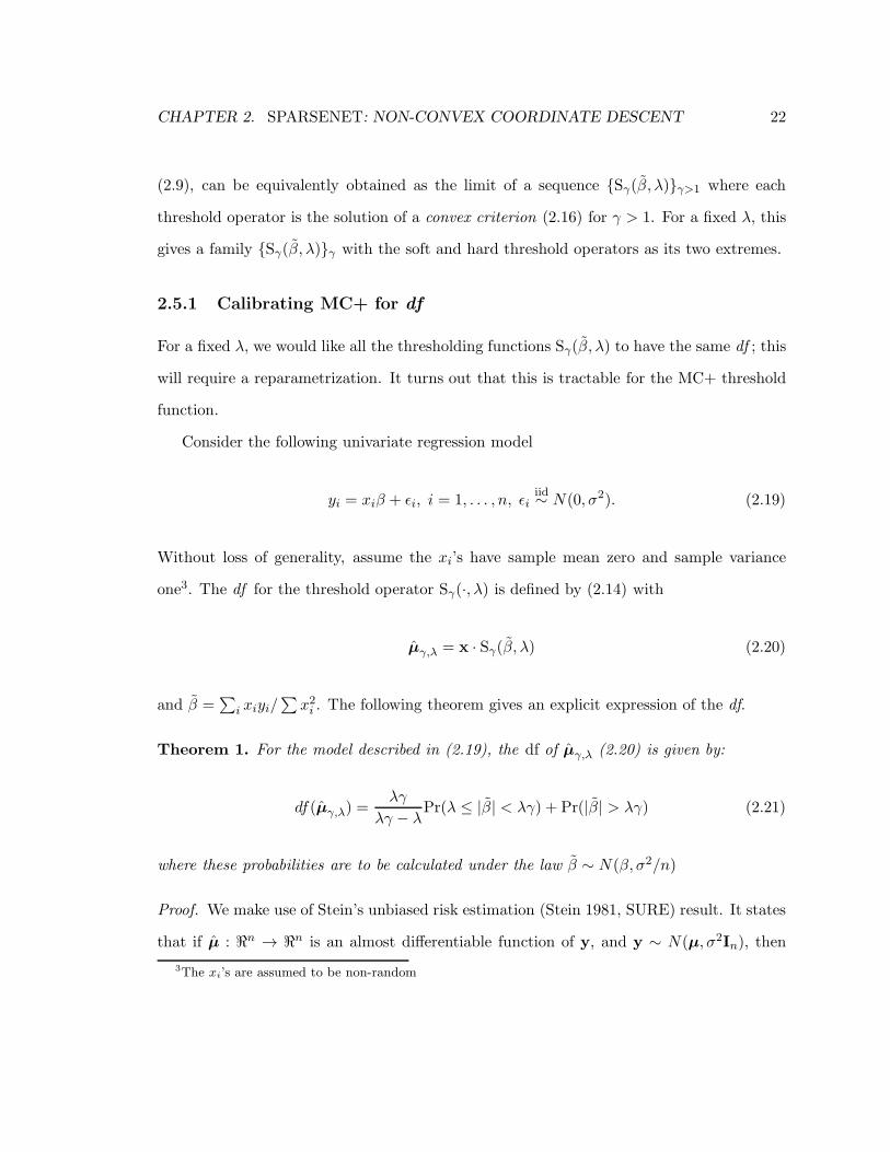
2.5.1 Calibrating MC+ for df
For a fixed λ, we would like all the thresholding functions Sγ(β, λ) to have the same df ; this
will require a reparametrization. It turns out that this is tractable for the MC+ threshold
function.
Consider the following univariate regression model
yi = xiβ + ǫi, i = 1, . . . , n, ǫiiid∼ N(0, σ2). (2.19)
Without loss of generality, assume the xi’s have sample mean zero and sample variance
one3. The df for the threshold operator Sγ(·, λ) is defined by (2.14) with
µγ,λ = x · Sγ(β, λ) (2.20)
and β =∑
i xiyi/∑
x2i . The following theorem gives an explicit expression of the df.
Theorem 1. For the model described in (2.19), the df of µγ,λ (2.20) is given by:
df(µγ,λ) =λγ
λγ − λPr(λ ≤ |β| < λγ) + Pr(|β| > λγ) (2.21)
where these probabilities are to be calculated under the law β ∼ N(β, σ2/n)
Proof. We make use of Stein’s unbiased risk estimation (Stein 1981, SURE) result. It states
that if µ : ℜn → ℜn is an almost differentiable function of y, and y ∼ N(µ, σ2In), then
3The xi’s are assumed to be non-random

CHAPTER 2. SPARSENET: NON-CONVEX COORDINATE DESCENT 23
there is a simplification to the df(µ) formula (2.14)
df(µ) =n∑
i=1
Cov(µi, yi)/σ2
= E(∇ · µ), (2.22)
where ∇ · µ =∑n
i=1 ∂µi/∂yi. Proceeding along the lines of proof in Zou et al. (2007), the
function µγ,λ : ℜ → ℜ defined in (2.20) is uniformly Lipschitz (for every λ ≥ 0, γ > 1), and
hence almost everywhere differentiable. The result follows easily from the definition (2.17)
and that of β, which leads to (2.21).
As γ →∞, µγ,λ → µλ, and from (2.21), we see that
df(µγ,λ) −→ Pr(|β| > λ) (2.23)
= E (I(|β| > 0))
which corresponds to the expression obtained by Zou et al. (2007) for the df of the LASSO
in the univariate case.
Corollary 1. The df for the hard-thresholding function H(β, λ) is given by
df(µ1+,λ) = λφ∗(λ) + Pr(|β| > λ) (2.24)
where φ∗ is taken to be the p.d.f. of the absolute value of a normal random variable with
mean β and variance σ2/n.
For the hard threshold operator, Stein’s simplified formula does not work, since the
corresponding function y 7→ H(β, λ) is not almost differentiable. But observing from (2.21)
that
df(µγ,λ)→ λφ∗(λ) + Pr(|β| > λ), and Sγ(β, λ)→ H(β, λ) as γ → 1+ (2.25)

CHAPTER 2. SPARSENET: NON-CONVEX COORDINATE DESCENT 24
we get an expression for df as stated.
These expressions are consistent with simulation studies based on Monte Carlo estimates
of df. Figure 2.4[Left] shows df as a function of γ for a fixed value λ = 1 for the uncalibrated
MC+ threshold operators Sγ(·, λ). For the figure we used β = 0 and σ2 = 1.
Re-parametrization of the MC+ penalty
We argued in Section 2.4.2 that for the df to remain constant for a fixed λ and varying γ,
the shrinkage threshold λS = λS(λ, γ) should increase as γ moves from γ1 to γ0. Theorem
3 formalizes this observation.
Hence for the purpose of df calibration, we re-parametrize the family of penalties as
follows:
λP ∗(|t|;λ; γ) = λS(λ, γ)
∫ |t|
0
(1−
x
γλS(λ, γ)
)
+
dx. (2.26)
With the re-parametrized penalty, the thresholding function is the obvious modification
of (2.17):
S∗γ(β, λ) = argminβ12(β − β)2 + λP ∗(|β|;λ; γ)
= Sγ(β, λS(λ, γ)) (2.27)
Similarly for the df we simply plug into the formula (2.21)
df(µ∗γ,λ) =
γλS(λ, γ)
γλS(λ, γ) − λS(λ, γ)Pr(λS(λ, γ) ≤ |β| < γλS(λ, γ)) + Pr(|β| > γλS(λ, γ))
(2.28)
where µ∗γ,λ = µγ,λS(λ,γ).
To achieve a constant df, we require the following to hold for λ > 0:
• The shrinkage-threshold for the soft threshold operator is λS(λ, γ = ∞) = λ and
hence µ∗λ = µλ ( a boundary condition in the calibration).

CHAPTER 2. SPARSENET: NON-CONVEX COORDINATE DESCENT 25
• df(µ∗γ,λ) = df(µλ) ∀ γ > 1.
The definitions for df depend on β and σ2/n. Since the notion of df centers around variance,
we use the null model with β = 0. We also assume without loss of generality that σ2/n = 1,
since this gets absorbed into λ.
Theorem 2. For the calibrated MC+ penalty to achieve constant df, the shrinkage-threshold
λS = λS(λ, γ) must satisfy the following functional relationship
Φ(γλS)− γΦ(λS) = −(γ − 1)Φ(λ), (2.29)
where Φ is the standard normal cdf and φ the pdf of the same.
Theorem 2 is proved in the secondary Appendix 2.2.1, using (2.28) and the bound-
ary constraint. The next theorem establishes some properties of of the map (λ, γ) 7→
(λS(λ, γ), γλS(λ, γ)), including the important nesting of shrinkage thresholds.
Theorem 3. For a fixed λ,
(a) γλS(λ, γ) is increasing as a function of γ.
(b) λS(λ, γ) is decreasing as a function of γ
Note that as γ increases, we approach the LASSO; see Figure 2.4 (right). Both these
relationships can be derived from the functional equation (2.29). Theorem 3 is proved in
the secondary Appendix 2.2.1.
Efficient computation of shrinkage thresholds
In order to implement the calibration for MC+, we need an efficient method for evaluating
λS(λ, γ)—i.e. solving equation (2.29). For this purpose we propose a simple parametric form
for λS based on some of its required properties: the monotonicity properties just described,

CHAPTER 2. SPARSENET: NON-CONVEX COORDINATE DESCENT 26
and the df calibration. We simply give the expressions here, and leave the details for the
secondary Appendix 2.2.2:
λS(λ, γ) = λH(1− α∗
γ+ α∗) (2.30)
where
α∗ = λ−1H Φ−1(Φ(λH)− λHφ(λH)), λ = λHα∗ (2.31)
The above approximation turns out to be a reasonably good estimator for all practical
purposes, achieving a calibration of df within an accuracy of five percent, uniformly over
all (γ, λ). The approximation can be improved further, if we take this estimator as the
starting point, and obtain recursive updates for λS(λ, γ). Details of this approximation
along with the algorithm are explained in the secondary Appendix 2.2.2. Numerical studies
show that a few iterations of this recursive computation can improve the degree of accuracy
of calibration up to an error of 0.3 percent; Figure 2.4 [Left] was produced using this
approximation. Figure 2.5 shows a typical pattern of recalibration for the example we
present in Figure 2.7 in Section 2.8.
0.0 0.2 0.4 0.6 0.8 1.0 1.2 1.4
12
510
2050
γ
λS(γ, λ)
Figure 2.5: Recalibrated values of λ via λS(γ, λ) for the MC+ penalty. The values of λ at thetop of the plot correspond to the LASSO. As γ decreases, the calibration increases the shrinkagethreshold to achieve a constant univariate df.

CHAPTER 2. SPARSENET: NON-CONVEX COORDINATE DESCENT 27
As noted below Algorithm 1 this leads to a lattice of values λk,ℓ.
2.6 Convergence Analysis
In this section we present results on the convergence of Algorithm 1. Tseng & Yun (2009)
show convergence of coordinate-descent for functions that can be written as the sum of a
smooth function (loss) and a separable non-smooth convex function (penalty). This is not
directly applicable to our case as the penalty is non-convex.
Denote the coordinate-wise updates βk+1 = Scw(βk), k = 1, 2, . . . with
βk+1j = argmin
uQ(βk+1
1 , . . . , βk+1j−1 , u, β
kj+1, . . . , β
kp ), j = 1, . . . , p. (2.32)
Theorem 4 establishes that under certain conditions, SparseNet always converges to a min-
imum of the objective function; conditions that are met, for example, by the SCAD and
MC+ penalties (for suitable γ).
Theorem 4. Consider the criterion in (2.6), where the given data (y,X) lies on a compact
set and no column of X is degenerate (ie multiple of the unit vector). Suppose the penalty
λP (t;λ; γ) ≡ P (t) satisfies P (t) = P (−t), P ′(|t|) is non-negative, uniformly bounded and
inft P′′(|t|) > −1; where P ′(|t|) and P ′′(|t|) are the first and second derivatives (assumed to
exist) of P (|t|) wrt |t|.
Then the univariate maps β 7→ Q(1)(β) are strictly convex and the sequence of coordinate-
updates βkk converge to a minimum of the function Q(β).
Note that the condition on the data (y,X) is a mild assumption (as it is necessary for
the variables to be standardized). Since the columns of X are mean-centered, the non-
degeneracy assumption is equivalent to assuming that no column is identically zero.
The proof is provided in Appendix 2.A.1. Lemma 1 and Lemma 3 under milder regularity
conditions, establish that every limit point of the sequence βk is a stationary point of

CHAPTER 2. SPARSENET: NON-CONVEX COORDINATE DESCENT 28
Q(β).
Remark 1. Note that Theorem 4 includes the case where the penalty function P (t) is convex
in t.
2.7 Simulation Studies
In this section we compare the simulation performance of a number of different methods
with regard to a) prediction error, b) the number of non-zero coefficients in the model, and c)
“misclassification error” of the variables retained. The methods we compare are SparseNet,
Local Linear Approximation (LLA) and Multi-stage Local Linear Approximation (MLLA)
(Zou & Li 2008, Zhang 2009, Candes et al. 2008), LASSO, forward-stepwise regression and
best-subset selection. Note that SparseNet, LLA and MLLA are all optimizing the same
MC+ penalized criterion.
We assume a linear model Y = Xβ + ε with multivariate Gaussian predictors X and
Gaussian errors. The Signal-to-Noise Ratio (SNR) and Standardized Prediction Error (SPE)
are defined as
SNR =
√βTΣβ
σ, SPE =
E(y − xβ)2
σ2(2.33)
The minimal achievable value for SPE is 1 (the Bayes error rate). For each model, the
optimal tuning parameters — λ for the penalized regressions, subset size for best-subset
selection and stepwise regression—are chosen based on minimization of the prediction error
on a separate large validation set of size 10K. We use SNR=3 in all the examples.
Since a primary motivation for considering non-convex penalized regressions is to mimic
the behavior of best subset selection, we compare its performance with best-subset for small
p = 30. For notational convenience Σ(ρ;m) denotes am×mmatrix with 1’s on the diagonal,
and ρ’s on the off-diagonal.
We consider the following examples:

CHAPTER 2. SPARSENET: NON-CONVEX COORDINATE DESCENT 29
S1: small p1.
01.
52.
02.
53.
0
Prediction Error
SN
R=
3
−−−−−− −−−
bs st 1 3 4 las
LLAMLLASparseNet
010
2030
40
% of Non−zero coefficients
SN
R=
3
−
−
−−−
bs st 1 3 4 las
0.00
0.05
0.10
0.15
0.20
0.25
0.30
0−1 Error
SN
R=
3
−−−
−−−−−−
bs st 1 3 4 las
γγγ
M1: moderate p
1.0
1.5
2.0
2.5
3.0
Prediction Error
SN
R=
3
−−− −−−
st 0.4 1 3 4 las
LLAMLLASparseNet
010
2030
40
% of Non−zero coefficients
SN
R=
3
−−−
−−−
st 0.4 1 2 3 4 5 las
0.00
0.05
0.10
0.15
0.20
0.25
0.30
0−1 Error
SN
R=
3
−−−−−−
st 0.4 1 3 4 las
γγγ
Figure 2.6: Examples S1 and M1. The three columns of plots represent prediction error, recoveredsparsity and zero-one loss (all with standard errors over the 25 runs). Plots show the recalibratedMC+ family for different values of γ (on the log-scale) via SparseNet, LLA, MLLA, LASSO (las),step-wise (st) and best-subset (bs) (for S1 only)

CHAPTER 2. SPARSENET: NON-CONVEX COORDINATE DESCENT 30
S1: n = 35, p = 30, ΣS1 = Σ(0.4; p) and βS1 = (0.03, 0.07, 0.1, 0.9, 0.93, 0.97, 01×24).
M1: n = 100, p = 200, ΣM1 = 0.7|i−j|1≤i,j≤p and βM1 has 10 non-zeros such that
βM1
20i+1 = 1, i = 0, 1, . . . , 9; and βM1
i = 0 otherwise.
In example M1 best-subset was not feasible and hence was omitted. The starting point for
both LLA and MLLA were taken as a vector of all ones (Zhang 2009). Results are shown
in Figure 2.6 with discussion in Section 2.7.1. These two examples, chosen from a battery
of similar examples, show that SparseNet compares very favorably with its competitors.
We now consider some larger examples and study the performance of SparseNet varying
γ.
M1(5): n = 500, p = 1000, ΣM1(5) = blockkdiag(ΣM1 , . . . ,ΣM1) and βM1(5) = (βM1 , . . . ,βM1)
(five blocks).
M1(10): n = 500, p = 2000 (same as above with ten blocks instead of five).
M2(5): n = 500, p = 1000, ΣM2(5) = blockdiag(Σ(0.5, 200), . . . ,Σ(0.5, 200)) and βM2(5) =
(βM2 , . . . ,βM2) (five blocks). Here βM2 = (β1, β2, . . . , β10,01×190) is such that the
first ten coefficients form an equi-spaced grid on [0, 0.5].
M2(10): n = 500, p = 2000, and is like M2(5) with ten blocks.
The results are summarized in Table 2.1, with discussion in Section 2.7.1.
2.7.1 Discussion of Simulation Results
In both S1 and M1, the aggressive non-convex SparseNet out-performs its less aggressive
counterparts in terms of prediction error and variable selection. Due to the correlation
among the features, the LASSO and the less aggressive penalties estimate a considerable
proportion of zero coefficients as non-zero. SparseNet estimates for γ ≈ 1 are almost iden-
tical to the best-subset procedure in S1. Step-wise performs worse in both cases. LLA and

CHAPTER 2. SPARSENET: NON-CONVEX COORDINATE DESCENT 31
log(γ) valuesExample: M1(5) 3.92 1.73 1.19 0.10
SPE 1.6344(9.126e−4) 1.3194(5.436e−4) 1.2015(4.374e−4) 1.1313(3.654e−4)
% of non-zeros [5] 16.370(0.1536) 13.255(0.1056) 8.195(0.0216) 5.000(0.0)0− 1 error .1137(1.536e−3) .0825(1.056e−3) .0319(.724e−3) .0002(.087e−3)
Example: M2(5)SPE 1.3797(0.486e−3) 1.467(0.531e−3) 1.499(7.774e−3) 1.7118(0.918e−3)
% of non-zeros [5] 21.435(0.1798) 9.900(0.1156) 6.74(0.097) 2.490(0.0224)0− 1 error 0.18445(1.63e−3) 0.08810(1.428e−3) 0.0592(0.841e−3) 0.03530(0.571e−3)
Example: M1(10)SPE 3.6819(0.58e−2) 4.4838(0.99e−2) 4.653(1.033e−2) 5.4729(2.006e−2)
% of non-zeros [5] 22.987(0.103) 11.9950(0.075) 8.455(0.0485) 6.2625(0.0378)0− 1 error 0.1873(1.172e−3) 0.0870(1.113e−3) 0.0577(1.191e−3) 0.0446(1.473e−3)
Example: M2(10)SPE 1.693(.906e−3) 1.893(.756e−3) 2.318(1.383e−3) 2.631(1.638e−2)
% of non-zeros [5] 15.4575(0.128) 8.2875(0.066) 5.6625(0.059) 2.22(0.0214)0− 1 error 0.1375(1.384e−3) 0.0870(1.1e−3) 0.0678(0.554e−3) 0.047(0.486e−3)
Table 2.1: Table showing standardized prediction error (SPE), percentage of non-zeros and zero-one error in the recovered model via SparseNet, for different problem instances. Values withinparenthesis (in subscripts) denote the standard errors, and the true number of non-zero coefficientsin the model are in square braces. Results are averaged over 25 runs.

CHAPTER 2. SPARSENET: NON-CONVEX COORDINATE DESCENT 32
MLLA show similar behavior in S1, but are inferior to SparseNet in predictive performance
for smaller values of γ. This shows that MLLA and SparseNet reach very different local
optima. In M1 LLA/MLLA seem to show similar behavior across varying degrees of non-
convexity. This is undesirable behavior, and is probably because MLLA/LLA gets stuck in
a local minima. MLLA does perfect variable selection and shows good predictive accuracy.
In M1(5), (n = 500, p = 1000) the prediction error decreases steadily with decreasing
γ, the variable selection properties improve as well. In M1(10) (n = 500, p = 2000) the
prediction error increases overall, and there is a trend reversal — with the more aggressive
non-convex penalties performing worse. The variable selection properties of the aggressive
penalties, however, are superior to its counterparts. The less aggressive non-convex selec-
tors include a larger number of variables with high shrinkage, and hence perform well in
predictive accuracy.
In M2(5) and M2(10), the prediction accuracy decreases marginally with increasing
γ. However, as before, the variable selection properties of the more aggressive non-convex
penalties are far better.
In summary, SparseNet is able to mimic the prediction performance of best subset
regression in these examples. In the high-p settings, it repeats this behavior, mimicking
the best, and is the out-right winner in several situations since best-subset regression is not
available. In situations where the less aggressive penalties do well, SparseNet often reduces
the number of variables for comparable prediction performance, by picking a γ in the interior
of its range. The solutions of LLA and MLLA are quite different from the SparseNet and
they often show similar performances across γ (as also pointed out in Candes et al. (2008)
and Zou & Li (2008)).
It appears that the main differences among the different strategies MLLA, LLA and
SparseNet lie in their roles of optimizing the objective Q(β). We study this from a well
grounded theoretical framework in Section 2.8, simulation experiments in Section 2.8.1 and
further examples in Section 2.2.3 in the secondary appendix.

CHAPTER 2. SPARSENET: NON-CONVEX COORDINATE DESCENT 33
2.8 Other methods of optimization
We shall briefly review some of the state-of-the art methods proposed for optimization with
general non-convex penalties.
Fan & Li (2001) used a local quadratic approximation (LQA) of the SCAD penalty.
The method can be viewed as a majorize-minimize algorithm which repeatedly performs
a weighted ridge regression. LQA gets rid of the non-singularity of the penalty at zero,
depends heavily on the initial choice β0, and is hence suboptimal (Zou & Li 2008) in
searching for sparsity.
The MC+ algorithm of Zhang (2010) cleverly tracks multiple local minima of the objec-
tive function and seeks a solution to attain desirable statistical properties. The algorithm is
complex, and since it uses a LARS-type update, is potentially slower than coordinate-wise
procedures.
Friedman (2008) proposes a path-seeking algorithm for general non-convex penalties.
Except in simple cases, it is unclear what criterion of the form “loss+penalty” it optimizes.
Multi-stage Local Linear Approximation. Zou & Li (2008), Zhang (2009) and Candes
et al. (2008) propose majorize-minimize (MM) algorithms for minimization of Q(β) (2.6),
and consider the re-weighted ℓ1 criterion
Q(β;βk) = Constant + 12‖y −Xβ‖2 + λ
p∑
j=1
P ′(|βkj |;λ; γ)|βj | (2.34)
for some starting point β1. If βk+1 is obtained by minimizing (2.34)— we denote the update
via the map βk+1 := Mlla(βk). There is currently a lot of attention payed to MLLA in the
literature, so we analyze and compare it to our coordinate-wise procedure in more detail.
We have observed (Sections 2.8.1 and 2.2.3) that the starting point is critical; see also
Candes et al. (2008) and Zhang (2010). Zou & Li (2008) suggest stopping at k = 2 after
starting with an “optimal” estimator, for example, the least-squares estimator when p < n.
CHAPTER 2. SPARSENET: NON-CONVEX COORDINATE DESCENT 34
Choosing an optimal initial estimator β1 is essentially equivalent to knowing a-priori the
zero and non-zero coefficients of β. The adaptive LASSO of Zou (2006) is very similar in
spirit to this formulation, though the weights (depending upon a good initial estimator) are
allowed to be more general than derivatives of the penalty (2.34).
Convergence properties of SparseNet and MLLA can be analyzed via properties of fixed
points of the maps Scw(·) and Mlla(·) respectively. If the sequences produced by Mlla(·) or
Scw(·) converge, they correspond to stationary points of the function Q. Fixed points of the
maps Mlla(·) and Scw(·) correspond to convergence of the sequence of updates.
The convergence analysis of MLLA is based on the fact that Q(β;βk) majorizes Q(β).
If βk is the sequence produced via MLLA, then Q(βk)k≥1 converges. This does not
address the convergence properties of βkk≥1 nor properties of its limit points. Zou &
Li (2008) point out that if the map Mlla satisfies Q(β) = Q(Mlla(β)) for limit points of
the sequence βkk≥1, then the limit points are stationary points of the function Q(β).
It appears, however, that solutions of Q(β) = Q(Mlla(β)) are not easy to characterize by
explicit regularity conditions on the penalty P . The analysis does not address the fate of
all the limit points of the sequence βkk≥1 in case the sufficient conditions of Proposition
1 in Zou & Li (2008) fail to hold true. Our analysis in Section 2.6 for SparseNet addresses
all the concerns raised above. Fixed points of the map Scw(·) are explicitly characterized
through some regularity conditions of the penalty functions as described in Section 2.6.
Explicit convergence can be shown under additional conditions — Theorem 4.
Furthermore, a fixed point of the map Mlla(·) need not be a fixed point of Scw(·) – for
specific examples see Section 2.2.3 in the secondary appendix. Every stationary point of
the coordinate-wise procedure, however, is also a fixed point of MLLA.
The formal framework being laid, we proceed to perform some simple numerical ex-
periments in Section 2.8.1. Further discussions and comparisons between coordinate-wise
procedures and MLLA can be found in Section 2.2.3 in the secondary appendix.

CHAPTER 2. SPARSENET: NON-CONVEX COORDINATE DESCENT 35
2.8.1 Empirical performance and the role of calibration
In this section we show the importance of calibration and the specific manner in which
the regularization path is traced out via SparseNet in terms of the quality of the solution
obtained. In addition we compare the optimization performance of LLA/MLLA versus
SparseNet.
In Figure 2.7 we consider an example with n = p = 10, Σ = 0.8|i−j|1 ≤ i, j,≤ p,
SNR=1, β1 = βp = 1, all other βj = 0. We consider 50 values of γ and 20 values of λ, and
compute the solutions for all methods at the recalibrated pairs (γ, λS(γ, λ)); see Figure 2.5
for the exact λk,ℓ values used in these plots.
0.0 0.2 0.4 0.6
0.0
0.2
0.4
0.6
0.8
1.0
Sparsenet
0.0 0.2 0.4 0.6
0.0
0.2
0.4
0.6
0.8
1.0
Type (a)
0.0 0.2 0.4 0.6
0.0
0.2
0.4
0.6
0.8
1.0
Type(b)
0.0 0.2 0.4 0.6
0.0
0.2
0.4
0.6
0.8
1.0
Type(c)
Obj
ectiv
e
γ = 70γ = 13γ = 6γ = 1+
λλλλ
0.0 0.2 0.4 0.6
1.0
1.5
2.0
2.5
3.0
3.5
1.09
0.0 0.2 0.4 0.6
1.0
1.5
2.0
2.5
3.0
3.5
1.06
0.0 0.2 0.4 0.6
1.0
1.5
2.0
2.5
3.0
3.5
1.54
λλλ
I(γ,λ
)
Figure 2.7: Top row: objective function for SparseNet compared to other coordinate-wise variants— Type (a), (b) and MLLA Type (c) — for a typical example. Plots are shown for 50 values of γ(some are labeled in the legend) and at each value of γ, 20 values of λ. Bottom row: relative increaseI(γ, λ) in the objective compared to SparseNet, with the average I reported at the top of each plot.

CHAPTER 2. SPARSENET: NON-CONVEX COORDINATE DESCENT 36
a b c1.
01.
52.
02.
5
% In
crea
se in
Obj
ectiv
e
Figure 2.8: Boxplots of I over 24 different examples. In all cases SparseNet shows superior perfor-mance.
We compare SparseNet with
Type (a) Coordinate-wise procedure that computes solutions on a grid of λ for every fixed
γ, with warm-starts across λ (from larger to smaller values). No df calibration is used
here.
Type (b) Coordinate-wise procedure “cold-starting” with a zero vector (She 2009) for
every pair (λ, γ).
Type (c) MLLA with the starting vector initialized to a vector of ones (Zhang 2009).
In all cases SparseNet shows superior performance. For each (γ, λ) pair we compute the
relative increase I(γ, λ) = [Q(β∗)+0.05]/[Q(βs)+0.05], where Q(β∗) denotes the objective
value obtained for procedure ∗ (types (a), (b) or (c) above), andQ(βs) represents SparseNet.
These values are shown in the second row of plots. They are also averaged over all values
of (γ, λ) to give I (shown at the top of each plot). This is one of 24 different examples, over
6 different problem set-ups with 4 replicates in each. Figure 2.8 summarizes I for these 24
scenarios. Results are shown in Figure 2.74 The figure shows clearly the benefits of using the
proposed calibration in terms of optimization performance. MLLA appears to get “stuck”
4We show the curves of the objective values, as in Figure 2.7, for all 24 scenarios in the secondaryAppendix.

CHAPTER 2. SPARSENET: NON-CONVEX COORDINATE DESCENT 37
in local optima, supporting our claim in section 2.7.1. For larger values of γ the different
coordinate-wise procedures perform similarly, since the problem is close to convex.
2.A Primary Appendix to Chapter 2
2.A.1 Convergence Analysis for Algorithm 1
To prove Theorem 4 we require Lemma 1.
Lemma 1. Suppose the data (y,X) lies on a compact set. In addition, we assume the
following
1. The penalty function P (t) (symmetric around 0) is differentiable on t ≥ 0; P ′(|t|)
is non-negative, continuous and uniformly bounded, where P ′(|t|) is the derivative of
P (|t|) wrt |t|.
2. The sequence generated βkk is bounded
3. For every convergent subsequence βnkk ⊂ βkk the successive differences converge
to zero: βnk − βnk−1 → 0
If β∞ is any limit point of the sequence βkk, then β∞ is a minimum for the function
Q(β); i.e. for any δ = (δ1, . . . , δp) ∈ ℜp
lim infα↓0+
Q(β∞ + αδ)−Q(β∞)
α
≥ 0 (2.35)
In the secondary Appendix 2.2 we present the proof of Lemma 1. We also show via
Lemma 2 that assumption 2 is by no means restrictive. Lemma 3 gives a sufficient condition
under which assumption 3 of Lemma 1 is true.
It is useful to note here that assumptions 2, 3 of Lemma 1 follow from the assumptions
of Theorem 4 (we make a further note of this in the proof below).
We are now in a position to present the proof of Theorem 4:

CHAPTER 2. SPARSENET: NON-CONVEX COORDINATE DESCENT 38
Proof. Proof of Theorem 4 We will assume WLOG that the data is standardized.
For fixed i and (β1, . . . , βi−1, βi+1, . . . , βp), we will write χi(β1,...,βi−1,βi+1,...,βp)
≡ χ(u) for
the sake notational convenience.
The sub-gradient(s) (Borwein & Lewis 2006) of χ(u) at u are given by
∂χ(u) = ∇if((β1, . . . , βi−1, u, βi+1, . . . , βp)) + P ′(|u|) sgn(u) (2.36)
Also observe that
χ(u+ δ) − χ(u) =f((β1, . . . , βi−1, u+ δ, βi+1, . . . , βp))−
f((β1, . . . , βi−1, u, βi+1, . . . , βp)) + P (|u+ δ|) − P (|u|) (2.37)
=∇if((β1, . . . , βi−1, u, βi+1, . . . , βp))δ +12∇
2i fδ
2
+P ′(|u|)(|u + δ| − |u|) + 12P
′′(|u∗|)(|u+ δ| − |u|)2 (2.38)
Line (2.38) is obtained from (2.37) by a Taylor’s series expansions on f (wrt to the ith
coordinate) and |t| 7→ P (|t|). ∇2i f is the second derivative of the function f wrt the ith
coordinate and equals 1 as the features are all standardized; |u∗| is some number between
|u+ δ| and |u|. The rhs of (2.38) can be simplified as follows:
∇if((β1, . . . , βi−1, u, βi+1, . . . , βp))δ +12∇
2i fδ
2
+P ′(|u|)(|u + δ| − |u|) + 12P
′′(|u∗|)(|u + δ| − |u|)2
= 12∇
2i fδ
2 + ∇if((β1, . . . , βi−1, u, βi+1, . . . , βp))δ + P ′(|u|) sgn(u)δ+
P ′(|u|)(|u + δ| − |u|)− P ′(|u|) sgn(u)δ + 12P
′′(|u∗|)(|u+ δ| − |u|)2
(2.39)
Since χ(u) is minimized at u0; 0 ∈ ∂χ(u0). Thus using (2.36) we get
∇if((β1, . . . , βi−1, u0, βi+1, . . . , βp))δ + P ′(|u0|) sgn(u0)δ = 0 (2.40)

CHAPTER 2. SPARSENET: NON-CONVEX COORDINATE DESCENT 39
if u0 = 0 then the above holds true for some value of sgn(u0) ∈ [−1, 1].
By definition of sub-gradient of x 7→ |x| and P ′(|x|) ≥ 0 we have
P ′(|u|)(|u + δ| − |u|)− P ′(|u|) sgn(u)δ = P ′(|u|) ((|u+ δ| − |u|)− sgn(u)δ) ≥ 0 (2.41)
Using (2.40,2.41) in (2.39,2.38) at u = u0 we have
χ(u0 + δ)− χ(u0) ≥12∇
2i fδ
2 + 12P
′′(|u∗|)(|u0 + δ| − |u0|)2 (2.42)
Observe that (|u0 + δ| − |u0|)2 ≤ δ2.
If P ′′(|u∗|) ≤ 0 then 12P
′′(|u∗|)(|u0 + δ| − |u0|)2 ≥ 1
2P′′(|u∗|)δ2.
If P ′′(|u∗|) ≥ 0 then 12P
′′(|u∗|)(|u0 + δ| − |u0|)2 ≥ 0.
Combining these two we get
χ(u0 + δ)− χ(u0) ≥12δ
2(∇2
i f +minP ′′(|u∗|), 0)
(2.43)
By the conditions of this theorem, (∇2i f + infx P
′′(|x|)) > 0. Hence there exists a θ > 0,
θ = 12∇
2i f +mininf
xP ′′(|x|), 0 = 1
21 +mininfxP ′′(|x|), 0 > 0
which is independent of (β1, . . . , βi−1, βi+1, . . . , βp), such that
χ(u0 + δ)− χ(u0) ≥ θδ2 (2.44)
(For the MC+ penalty, infx P′′(|x|) = − 1
γ; γ > 1.
For the SCAD, infx P′′(|x|) = − 1
γ−1 ; γ > 2.)
In fact the dependence on u0 above in (2.44) can be further relaxed. Following the above
arguments carefully, we see that the function χ(u) is strictly convex (Borwein & Lewis 2006)

CHAPTER 2. SPARSENET: NON-CONVEX COORDINATE DESCENT 40
as it satisfies:
χ(u+ δ)− χ(u)− ∂χ(u)δ ≥ θδ2 (2.45)
We will use this result to show the convergence of βk . Using (2.44) we have
Q(βm−1i )−Q(βm−1
i+1 ) ≥ θ(βm−1i+1 − βm
i+1)2
= θ‖βm−1i − βm−1
i+1 ‖22 (2.46)
where βm−1i := (βm
1 , . . . , βmi , βm−1
i+1 , . . . , βm−1p ). (2.46) shows the boundedness of the se-
quence βm, for every m > 1 since the starting point β1 ∈ ℜp.
Using (2.46) repeatedly across every coordinate, we have for every m
Q(βm+1)−Q(βm) ≥ θ‖βm+1 − βm‖22 (2.47)
Using the fact that the (decreasing) sequence Q(βm) converges, it is easy to see from (2.47),
that the sequence βk cannot cycle without convergence ie it must have a unique limit point.
This completes the proof of convergence of βk.
Observe that, (2.47) implies that assumptions 2 and 3 of Lemma 1 are satisfied. Hence
using Lemma 1, the limit of βk is a minimum of Q(β) — this completes the proof.
2.2 Secondary Appendix to Chapter 2
We will first address the boundedness of the sequence βk. For this purpose we present the
following Lemma:
Lemma 2. Suppose the data (y,X) lies on a compact set. For fixed P (·;λ; γ) and β0 ∈ ℜp
let H′ = β|Q(β) ≤ Q(β0). There exists a bounded set H0 ⊂ ℜp such that
Q(β)|β ∈ H′ = Q(β)|β ∈ H0 (2.48)

CHAPTER 2. SPARSENET: NON-CONVEX COORDINATE DESCENT 41
Proof. This lemma is trivially true if P (|t|;λ; γ) is unbounded in |t|.
The lemma requires a proof if P (|t|;λ; γ) is uniformly bounded in |t| (MC+ penalty, for
example). We prove this part via contradiction.
Suppose there exists a sequence, βkk ⊂ H′ such that ‖βk‖2 → ∞. This necessarily
implies that, there is a subset of indices (i1, . . . , im) ⊂ 1, . . . , p such that (βki1, . . . , βk
im)k
is an unbounded sequence. This sequence satisfies (passing on to a subsequence if necessary),
X[i1, . . . , im](βki1, . . . , βk
im)′ = X[i1, . . . , im](β0
i1, . . . , β0
im)′
for some (β0i1, . . . , β0
im) ∈ ℜm independent of k and X[i1, . . . , im] = [xi1 , . . . ,xim ].
The sequence βkk ⊂ H′, considered above is arbitrary. Hence the range of values
taken by the function Q(β) remains the same if one restricts to bounded subsets of ℜp. So
there exists a bounded set H0 ⊂ ℜp such that (2.48) holds true.
Lemma 2, shows that the boundedness assumption on the coordinate-wise updates is
not by any means restrictive. If required, one can restrict ‖β‖∞ ≤M , in the Algorithm for
some M > 0, sufficiently large.
Lemmas 1 and 3 characterize the fate of limit points of the sequence produced by the
coordinate-wise updates under milder conditions than those required by Theorem 4.
Proof of Lemma 1
Proof. For any β = (β1, . . . , βp) and δi = (0, . . . , δi, . . . , 0) ∈ ℜp,
lim infα↓0+
Q(β + αδi)−Q(β)
α
= ∇if(β)δi + lim inf
α↓0+
P (|βi + αδi|)− P (|βi|)
α
(2.49)
where f(β) = 12‖y −Xβ‖22, ∇i is the partial derivative w.r.t. the ith coordinate.

CHAPTER 2. SPARSENET: NON-CONVEX COORDINATE DESCENT 42
Observe that the second term in (2.49) simplifies to
∂P (βi; δi) := lim infα↓0+
P (|βi + αδi|)− P (|βi|)
α
=
P ′(|βi|) sgn(βi)δi if |βi| > 0;
P ′(0)|δi| if |βi| = 0.(2.50)
where
sgn(x) ∈
1 if x > 0;
−1 if x < 0;
[-1,1] if x = 0.
Assume βnk → β∞ = (β∞1 , . . . , β∞
p ). Using (2.50) and Assumption 3, as k →∞
βnk−1i := (βnk
1 , . . . , βnk
i−1, βnk
i , βnk−1i+1 , βnk−1
p )→ (β∞1 , . . . , β∞
i−1, β∞i , β∞
i+1, β∞p ) (2.51)
If, β∞i 6= 0, ∂P (βnk
i ; δi)→ ∂P (β∞i ; δi); If, β∞
i = 0, ∂P (β∞i ; δi) ≥ lim inf
k∂P (βnk
i ; δi)
By definition of a coordinate-wise minimum, using (2.49,2.50) we have
∇if(βnk−1i )δi + ∂P (βnk
i ; δi) ≥ 0 ∀k (2.52)
The above imply ∀i ∈ 1, . . . , p
∇if(β∞)δi + ∂P (β∞
i ; δi) ≥ lim infk
∇if(β
nk−1i )δi + ∂P (βnk
i ; δi)≥︸︷︷︸
by (2.52)
0 (2.53)
Using (2.49,2.50) the l.h.s. of (2.53) gives
lim infα↓0+
Q(β∞ + αδ∞i )−Q(β∞)
α
≥ 0 (2.54)

CHAPTER 2. SPARSENET: NON-CONVEX COORDINATE DESCENT 43
For δ = (δ1, . . . , δp) ∈ ℜp, due to differentiability of f(β) = 1
2‖y −Xβ‖22
lim infα↓0+
Q(β∞ + αδ)−Q(β∞)
α
=
p∑
j=1
∇jf(β∞)δj +
p∑
j=1
limα↓0+
P (|β∞j + αδj |)− P (|β∞
j |)
α
=
p∑
j=1
f(β∞)δj + lim
α↓0+
P (|β∞j + αδj |)− P (|β∞
j |)
α
=
p∑
j=1
lim infα↓0+
Q(β∞ + αδ∞j )−Q(β∞)
α
≥︸︷︷︸
By (2.54)
0
(2.55)
This completes the proof.
Lemma 3 gives a sufficient condition under which Assumption 3 of Lemma 1 is true.
Lemma 3. Suppose in addition to Assumption 1 of Lemma 1 the following assumptions
hold:
1. For every i = 1, . . . , p and (u1, . . . , ui−1, ui+1, . . . , up) ∈ ℜp−1 the univariate function
χi(u1,...,ui−1,ui+1,...,up)
(·) : u 7→ Q(u1, . . . , ui−1, u, ui+1, . . . , up) (2.56)
has a unique global minimum.
2. If uG ≡ uG(u1, . . . , ui−1, ui+1, . . . , up) is the global minimum and
uL ≡ uL(u1, . . . , ui−1, ui+1, . . . , up) any other local minimum of the function (2.56);
there exists ǫ > 0, independent of the choice of (u1, . . . , ui−1, ui+1, . . . , up) such that
|uG(u1, . . . , ui−1, ui+1, . . . , up)− uL(u1, . . . , ui−1, ui+1, . . . , up)| ≥ ǫ
— that is uG and uL are uniformly separated.
Then for every convergent subsequence βnkk ⊂ βkk, the successive differences βnk −
βnk−1 → 0; i.e. Assumption 3 of Lemma 1 is true.

CHAPTER 2. SPARSENET: NON-CONVEX COORDINATE DESCENT 44
Proof. Borrowing notation from (2.51), consider the sequence βnk−1p−1
βnk−1p−1 := (βnk
1 , . . . , βnkp−2, β
nkp−1, β
nk−1p ) (2.57)
where βnk−1p−1 differs from βnk at the pth coordinate. We will show β
nk−1p−1 − βnk → 0 by the
method of contradiction.
Writing βnk − βnk−1p−1 = ∆nk
p := (0, . . . , 0,∆nkp ) we have
Q(βnk −∆nkp )−Q(βnk) ↓ 0 as nk →∞
As k →∞, let βnk → β+. Passing on to a subsequence (if necessary) we have ∆nkp → ∆+
p 6= 0
(as ∆nkp 9 0) and
βnk −∆nkp → β+ −∆+
p
Furthermore, the continuity of the function Q(·) implies
(Q(βnk −∆nk
p )−Q(βnk))↓(Q(β+ −∆+
p )−Q(β+))= 0 (2.58)
By the definition of βnk := (βnk1 , . . . , βnk
p ) we have
∇pf(βnk)δp + ∂P (βnk
p ; δp) ≥ 0, ∀k
Passing on to the limit k →∞ we get (using arguments as in proof of Lemma 1)
∇pf(β+)δp + ∂P (β+
p ; δp) ≥ 0
where β+ = (β+1 , . . . , β
+p ). This implies that χp
(β+1,...,β+
p−1)(u) has a minimum at u = β+
p . By
Assumption 2 of this Lemma the global minimum uG is uniformly separated from other local
minima uL — hence β+p is the global minimum. But (2.58) implies that χp
(β+1,...,β+
p−1)(u) has

CHAPTER 2. SPARSENET: NON-CONVEX COORDINATE DESCENT 45
two distinct global minima at u = β+p and u = β+
p −∆+p — a contradiction to Assumption
1. Hence ∆+p = 0 and βnk−1
p − βnkp → 0.
In the above spirit consider sequence (2.59) (differing from βnk−1p−1 at (p−1)th coordinate)
βnk−1p−2 := (βnk
1 , . . . , βnkp−3, β
nkp−2, β
nk−1p−1 , βnk−1
p ) (2.59)
We will show βnk−1p−2 − β
nk−1p−1 → 0, which along with β
nk−1p−1 − βnk → 0 (shown above) will
imply βnk−1p−2 − βnk → 0. The proof of this part is similar to the above.
Write βnk−1p−1 − β
nk−1p−2 = ∆nk−1
p−1 := (0, . . . , 0,∆nkp−1, 0) and suppose ∆nk
p−1 9 0. We will
arrive at a contradiction.
By hypothesis, there is a subsequence of ∆nkp−1 converging to ∆+
p−1 6= 0. Passing onto a
further subsequence, if necessary and using ∆nk−1p−1 →∆+
p−1 we have
(Q(βnk−1
p−1 −∆nk−1p−1 )−Q(βnk−1
p−1 ))↓(Q(β+ −∆+
p−1)−Q(β+))= 0 (2.60)
This essentially implies that the map χp−1
(β+1,...,β+
p−2,β+
p )(u) has two distinct global minima at
u = β+p−1 and u = β+
p−1 −∆+p−1; which is a contradiction — hence ∆nk
p−1 → 0.
We can follow the above arguments inductively for finitely many steps namely i =
p − 3, p − 4, . . . , 1, p and show that ∆nk
i → 0 for every i. This shows βnk−1 − βnk → 0,
thereby completing the proof.
The uniform separation condition — Assumption 2 of Lemma 3 is a trivial consequence
of strict convexity of the univariate functions (Theorem 4) and are more general.
2.2.1 Calibration of MC+ and Monotonicity Properties of λS, γλS
Proof of Theorem 2 on page 25

CHAPTER 2. SPARSENET: NON-CONVEX COORDINATE DESCENT 46
Proof. For convenience we rewrite λS(λ, γ) in terms of a function fλ(γ) as
λS(λ, γ) = λfλ(γ). (2.61)
Using (2.28) and the equality of effective df across all γ for every λ, fλ(γ) can be defined
as a solution to the following functional equation
γ
γ − 1Pr(λfλ(γ) ≤ |β| < γλfλ(γ)) + Pr(|β| > γλfλ(γ)) = Pr(|β| > λ) (2.62)
∀γ > 1, fλ(γ) > 1. (2.63)
Since we have assumed σ2/n = 1 and a null generative model, we have
γ
γ − 1(Φ(γλfλ(γ)) − Φ(λfλ(γ)) + (1− Φ(γλfλ(γ)) = (1− Φ(λ)) (2.64)
or equivalently
Φ(γλfλ(γ))− γΦ(λfλ(γ)) = −(γ − 1)Φ(λ) (2.65)
where Φ is the standard normal cdf and φ the pdf of the same. Equation (2.29) is obtained
from (2.65) and (2.61).
Proof of Theorem 3 on page 25 Before we begin the proof, we need a lemma.
Lemma 4. For δ ≤ λH , where λH = λS(λ, γ = 1+) the function h(δ)
h(δ) = Φ(δ)− Φ(λ)− δφ(δ) (2.66)
satisfies h(δ) < 0, ∀λH > δ > λ
Proof. Observe that for every fixed λ > 0, h(λ) = −δφ(δ) < 0. In addition, the derivative
of h(·) satisfies
h′(δ) = −δφ′(δ) > 0 (2.67)

CHAPTER 2. SPARSENET: NON-CONVEX COORDINATE DESCENT 47
since φ(δ) is the standard normal density and δ > 0.
Also, from equation (2.64) it follows that (taking γ → 1+),
λHφ(λH) + 1− Φ(λH) = 1− Φ(λ)
which implies Φ(λH)−Φ(λ)−λHφ(λH) = 0 that is h(λH) = 0. Since h(·) is strictly monotone
increasing on [λ, λH ], with h(λ) < 0 and h(λH) = 0 it is necessarily negative on [λ, λH).
This completes the proof.
Proof. Proof of part [a]. Let λ′max denote the partial derivative of λmax ≡ γλS(λ, γ) w.r.t
γ.
Differentiating both sides of equation (2.29) w.r.t γ, we get
λ′max(φ(γλS)− φ(λS)) = Φ(λS)− Φ(λ)− λSφ(λS) (2.68)
Observe that φ(γλS) < φ(λS), since γλS > λS .
In order to complete the proof it suffices to show that Φ(λS) − Φ(λ) − λSφ(λS) < 0.
This follows from Lemma 4, which gives h(λS) < 0 since λ < λS < λH .
Proof of part [b]. Let λ′min denote the partial derivative of λmin ≡ λS(λ, γ) w.r.t γ.
Differentiating both sides of equation (2.29) w.r.t γ, we get
λ′minγ(φ(γλS)− φ(λS)) = Φ(λS)− Φ(λ)− λSφ(γλS) (2.69)
Since φ(γλS) < φ(λS), it suffices to show that r.h.s of (2.69) is greater than zero. Define
for a fixed λ > 0 the function
g(λS , γ) = Φ(λS)− φ(γλS) (2.70)

CHAPTER 2. SPARSENET: NON-CONVEX COORDINATE DESCENT 48
From (2.29) it follows that,
Φ(λS) =γ − 1
γΦ(λ) + Φ(λSγ)/γ (2.71)
Using (2.71), g(λS , γ) becomes
g(λS , γ) = Φ(λ)−Φ(λ)
γ+
Φ(λSγ)
γ− φ(λSγ)λS (2.72)
Consider the function g(λS , γ)− Φ(λ), for fixed λ > 0.
By Theorem 3 (part [a]), we know that for fixed λ, the map γ 7→ λmax = γλS is increasing
in γ. Hence, the function g(λS , γ) − Φ(λ) is greater than zero iff the function h(u) (with
u = γλS)
h(u) = Φ(u)− uφ(u)− Φ(λ)
satisfies
h(u) > 0 on u > λH
Observe that h′(u) = −uφ′(u) > 0 on u > λH . In addition, from (2.64), taking limits over
γ it follows that h(λH) = 0.
This proves that h(u) > 0 on u > λH . Consequently, g(λS , γ) > Φ(λ) ∀γ > 1. This
proves that the r.h.s of (2.69) is greater than zero.
2.2.2 Parametric functional form for λS(λ, γ)
We detail out the steps leading to the expressions (2.30,2.31) given in Section 2.5.1.
For every fixed λ > 0 the following are the list of properties that the function fλ(γ) (see
Appendix 2.2.1) should have
1. monotone increase of shrinkage thresholds λS from soft to hard thresholding, implies
λfλ(γ) should be increasing as γ decreases.

CHAPTER 2. SPARSENET: NON-CONVEX COORDINATE DESCENT 49
2. monotone decrease of bias thresholds γλS from soft to hard thresholding requires
γλfλ(γ) to be increasing as γ increases.
3. The sandwiching property:
λS(γ) > λ ∀γ ∈ (1,∞) =⇒ fλ(γ) > 1 ∀γ ∈ (1,∞) (2.73)
4. The df calibration at the two extremes of the family: df(µγ=1+,λ) = df(µγ=∞,λ).
The above considerations suggest a nice parametric form for fλ(γ) given by
fλ(γ) = 1 + τ/γ for some τ > 0 (2.74)
Let us denote λS(λ, 1+) = λH
Equating the df ’s for the soft and hard thresholding τ is to be chosen as:
(1−Φ(λ)) = λHφ(λH) + (1− Φ(λH))
which implies
(1 + τ)−1 = fλ(γ = 1+) = λ−1H Φ−1(Φ(λH)− λHφ(λH))
Hence we get
λS = λH
(1
1 + τ+
τ
γ(1 + τ)
)
In addition, observe that as γ →∞, λS(λ, γ)→λH
1+τ= λ. This gives expression (2.31).
Tightening up the initial approximation of λS
In order to get a better approximation of the mapping (λ, γ) 7→ (λS , γλS), we can define
a sequence of recursive updates based on equation (2.29). Theorem 5 gives a proof of the

CHAPTER 2. SPARSENET: NON-CONVEX COORDINATE DESCENT 50
convergence of these updates and the algorithm for obtaining the better approximations are
given in Section (2.2.2).
Theorem 5. With reference to (2.29), define a sequence of estimates zkk≥0 recursively
as
1
γ − 1Φ(γzk)−
γ
γ − 1Φ(zk+1) = −Φ(λ) (2.75)
where the variables zkk≥0 are actually the iterative updates of λS(γ) for a fixed (λ, γ).
Under the condition
supk
|φ(ξ∗k)|
|φ(ξk)| < 1 (2.76)
where ξ∗k ∈ (minγzk, γzk+1,maxγzk, γzk+1) and ξk ∈ (minzk+1, zk+2,maxzk+1, zk+2)
for all k ≥ 0, the sequence zkk≥0 converges to a fixed point z∗ of the following equation:
1
γ − 1Φ(γz∗)−
γ
γ − 1Φ(z∗) = −Φ(λ) (2.77)
and hence provides a solution to (λ, γ) 7→ (λS(γ) = z∗, γλS(γ) = γz∗)
Proof. By the definition of the updates zk, in (2.75) we get for k = k, k + 1
1
γ − 1Φ(γzk)−
γ
γ − 1Φ(zk+1) = −Φ(λ) k ∈ k, k + 1
Using the above two we get:
Φ(γzk)− Φ(γzk+1) = γ(Φ(zk+1)− Φ(zk+2)) (2.78)
Applying the mean-value theorem on both sides of (2.78) we get:
(γzk − γzk+1)φ(γηk) = γ(zk+1 − zk+2)φ(η∗k) (2.79)
where ηk lies in between zk,zk+1 and η∗k lies in between zk+1,zk+2.

CHAPTER 2. SPARSENET: NON-CONVEX COORDINATE DESCENT 51
Writing Rk = φ(γηk)φ(η∗
k) , ∀k ≥ 0, we observe that
|zm+1 − zm+2| < C(supk
|Rk|)m
for some C which does not depend upon m. Suppose supk |Rk| < 1, then we observe that
the telescopic sum∑
k(zk+1 − zk) converges absolutely. Hence in particular the sequence
zk converges.
The condition (2.76) stated in this theorem, is a sufficient condition for supk |Rk| < 1,
hence the sequence of updates converge. Observe that, the sufficient condition is very
plausible since γ > 1, and the density φ(·) decreases on the positive reals.
This completes the proof.
Algorithm for tightening up the approximation of shrinkage thresholds
For a given (λ, γ) the re-parametrized MC+ penalty is of the form given in (2.26) where
λS , γλS defined through (2.29) are obtained by the following steps:
1. Obtain fλ(γ) based on the starting proposal function as in (2.75). This gives an
estimate for λmin and λmax = γλS using (2.61).
2. With z0 = λmin obtain recursively the sequence of estimates zkk≥1 using Theorem
(5) till convergence criterion is met, that is, |df(µγ,λ)− df(µγ=1+(y, λ))| < tol.
3. If the sequence zk → z∗ then assign λS = z∗ and γλS = γz∗
Theorem 5 gives a formal proof of the convergence of the above algorithm.
2.2.3 Understanding the sub-optimality of LLA through examples
In this section, as a continuation to Section 2.8 we explore the reasons behind the sub-
optimality of LLA through two univariate problem instances.

CHAPTER 2. SPARSENET: NON-CONVEX COORDINATE DESCENT 52
Example 1: log-penalty and the phase-transition phenomenon
Consider the log-penalized least-squares criterion (2.10)
Q(1)(β) = 12(β − β)2 +
λ
log(γ + 1)log(γ|β| + 1) (2.80)
for some large value of γ such that Q(1)(β) has multiple local minima, but a unique global
minimizer. The corresponding (multi-stage) LLA for this problem leads to a sequence
βkk≥1 defined by
βk+1 = argminβ
12(β − β)2 + wk|β|
= S(β, wk), with wk =λγ
(γ|βk|+ 1) log(γ + 1)(2.81)
Convergence of the sequence of estimates βk corresponds to fixed points of the function
Mlla : β 7→ sgn(β)(|β| −λ∗
(γ|β| + 1))+ with λ∗ =
λγ
log(γ + 1). (2.82)
Mlla(β) on β ≥ 0, has multiple fixed points for certain choices of λ, β.
For example, let γ = 500, λ = 74.6 and β = 10; here Q(β), β ≥ 0 has two minima, with
the global minimum at zero. Figure 2.9[Right] shows the iteration map Mlla(β). It has two
fixed points, corresponding to the two local minima 0 = β1 < β2 of Q(β), β ≥ 0. There
exists a critical value r > 0 such that
β1 < r =⇒ βk → 0 = β1, β1 > r =⇒ βk → β2 as k →∞ (2.83)
This phase transition phenomenon is responsible for the sub-optimality of the LLA in the
one-dimensional case. Note that the coordinate-wise procedure applied in this context will
give the global minimum.

CHAPTER 2. SPARSENET: NON-CONVEX COORDINATE DESCENT 53
The importance of the initial choice in obtaining “optimal” estimates via the re-weighted
ℓ1 minimization has also been pointed out in an asymptotic setting by Huang et al. (2008);
our observations are non-asymptotic.
−4 −2 0 2 4
02
46
810
Phase Transition for Log−penalty
FunctionConvergence PointPhase Transition
log(β)
Figure 2.9: Mlla(β) for the univariate log-penalized least squares problem. The starting point β1
determines which stationary point the LLA sequence will converge to. If the starting point is onthe right side of the phase transition line (vertical dotted line), then the LLA will converge to astrictly sub-optimal value of the objective function. In this example, the global minimum of theone-dimensional criterion is at zero.
Example 2: MC+ penalty and rate of convergence
Here we study the rate of convergence to the global minimum for the MC+ penalized least
squares problem (2.16). The multi-stage LLA for this problem gives the following updates
βk+1 = argminβ
12(β − β)2 + wk|β|
= S(β, wk), with wk = λ(1−|βk|
γλ)+ (2.84)
The function β 7→ S(β, λ(1− |βk|γλ
)+) need not be a contraction mapping, hence one cannot
readily appeal to Banach’s Fixed Point Theorem to obtain a proof of the convergence and
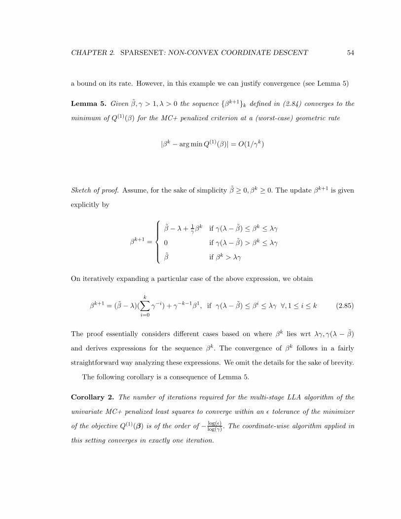
CHAPTER 2. SPARSENET: NON-CONVEX COORDINATE DESCENT 54
a bound on its rate. However, in this example we can justify convergence (see Lemma 5)
Lemma 5. Given β, γ > 1, λ > 0 the sequence βk+1k defined in (2.84) converges to the
minimum of Q(1)(β) for the MC+ penalized criterion at a (worst-case) geometric rate
|βk − argminQ(1)(β)| = O(1/γk)
Sketch of proof. Assume, for the sake of simplicity β ≥ 0, βk ≥ 0. The update βk+1 is given
explicitly by
βk+1 =
β − λ+ 1γβk if γ(λ− β) ≤ βk ≤ λγ
0 if γ(λ− β) > βk ≤ λγ
β if βk > λγ
On iteratively expanding a particular case of the above expression, we obtain
βk+1 = (β − λ)(
k∑
i=0
γ−i) + γ−k−1β1, if γ(λ− β) ≤ βi ≤ λγ ∀, 1 ≤ i ≤ k (2.85)
The proof essentially considers different cases based on where βk lies wrt λγ, γ(λ − β)
and derives expressions for the sequence βk. The convergence of βk follows in a fairly
straightforward way analyzing these expressions. We omit the details for the sake of brevity.
The following corollary is a consequence of Lemma 5.
Corollary 2. The number of iterations required for the multi-stage LLA algorithm of the
univariate MC+ penalized least squares to converge within an ǫ tolerance of the minimizer
of the objective Q(1)(β) is of the order of − log(ǫ)log(γ) . The coordinate-wise algorithm applied in
this setting converges in exactly one iteration.

CHAPTER 2. SPARSENET: NON-CONVEX COORDINATE DESCENT 55
Section 2.8.1, in the text describes empirical results and comparisons showing the per-
formance of SparseNet as an optimization algorithm. In the spirit of Figure 2.7, attached
below is a figure showing the objective value curves for all the 24 simulation examples.

Part II
Matrix Completion &
Collaborative Filtering
56

Chapter 3
Spectral Regularization Algorithms
Abstract: In this chaper, we use convex relaxation techniques to provide a sequence of regularized
low-rank solutions for large-scale matrix completion problems. Using the nuclear norm as a regular-
izer, we provide a simple and very efficient convex algorithm for minimizing the reconstruction error
subject to a bound on the nuclear norm. Our algorithm Soft-Impute iteratively replaces the miss-
ing elements with those obtained from a soft-thresholded SVD. With warm starts this allows us to
efficiently compute an entire regularization path of solutions on a grid of values of the regularization
parameter. The computationally intensive part of our algorithm is in computing a low-rank SVD
of a dense matrix. Exploiting the problem structure, we show that the task can be performed with
a complexity of order linear in the matrix dimensions. Our semidefinite-programming algorithm is
readily scalable to large matrices; for example Soft-Impute takes a few hours to compute low-rank
approximations of a 106 × 106 incomplete matrix with 107 observed entries, and fits a rank-95 ap-
proximation to the full Netflix training set in 3.3 hours. Our methods achieve good training and test
errors and exhibit superior timings when compared to other competitive state-of-the-art techniques.
This chapter is based on joint work with Trevor Hastie and Robert Tibshirani; and appears in
our paper Mazumder et al. (2010).
57
CHAPTER 3. SPECTRAL REGULARIZATION ALGORITHMS 58
3.1 Introduction
In many applications measured data can be represented in a matrix Xm×n, for which only
a relatively small number of entries are observed. The problem is to “complete” the matrix
based on the observed entries, and has been dubbed the matrix completion problem (Candes
& Recht 2008, Candes & Tao 2009, Rennie & Srebro 2005). The “Netflix” competition
(SIGKDD & Netflix 2007, for example,) is a popular example, where the data is the basis
for a recommender system. The rows correspond to viewers and the columns to movies,
with the entry Xij being the rating ∈ 1, . . . , 5 by viewer i for movie j. There are about
480K viewers and 18K movies, and hence 8.6 billion (8.6× 10⁹) potential entries. However,
on average each viewer rates about 200 movies, so only 1.2% or 108 entries are observed.
The task is to predict the ratings that viewers would give to movies they have not yet rated.
These problems can be phrased as learning an unknown parameter (a matrix Zm×n) with
very high dimensionality, based on very few observations. In order for such inference to be
meaningful, we assume that the parameter Z lies in a much lower dimensional manifold.
In this chapter, as is relevant in many real life applications, we assume that Z can be well
represented by a matrix of low rank, that is, Z ≈ Vm×kGk×n, where k ≪ min(n,m). In
this recommender-system example, low rank structure suggests that movies can be grouped
into a small number of “genres”, with Gℓj the relative score for movie j in genre ℓ. Viewer
i on the other hand has an affinity Viℓ for genre ℓ, and hence the modeled score for viewer i
on movie j is the sum∑k
ℓ=1 ViℓGℓj of genre affinities times genre scores. Typically we view
the observed entries in X as the corresponding entries from Z contaminated with noise.
Srebro, Alon & Jaakkola (2005) studied generalization error bounds for learning low-
rank matrices. Recently Candes & Recht (2008), Candes & Tao (2009), and Keshavan et al.
(2009) showed theoretically that under certain assumptions on the entries of the matrix,
locations, and proportion of unobserved entries, the true underlying matrix can be recovered
within very high accuracy.

CHAPTER 3. SPECTRAL REGULARIZATION ALGORITHMS 59
For a matrixXm×n let Ω ⊂ 1, . . . ,m×1, . . . , n denote the indices of observed entries.
We consider the following optimization problem:
minimize rank(Z)
subject to∑
(i,j)∈Ω(Xij − Zij)
2 ≤ δ, (3.1)
where δ ≥ 0 is a regularization parameter controlling the tolerance in training error. The
rank constraint in (3.1) makes the problem for general Ω combinatorially hard (Srebro
& Jaakkola 2003). For a fully-observed X on the other hand, the solution is given by
a truncated singular value decomposition (SVD) of X. The following seemingly small
modification to (3.1),
minimize ‖Z‖∗
subject to∑
(i,j)∈Ω(Xij − Zij)
2 ≤ δ, (3.2)
makes the problem convex (Fazel 2002). Here ‖Z‖∗ is the nuclear norm, or the sum of
the singular values of Z. Under many situations the nuclear norm is an effective convex
relaxation to the rank constraint (Fazel 2002, Candes & Recht 2008, Candes & Tao 2009,
Recht et al. 2007). Optimization of (3.2) is a semi-definite programming problem (Boyd &
Vandenberghe 2004) and can be solved efficiently for small problems, using modern convex
optimization software like SeDuMi and SDPT3 (Grant & Boyd. 2009). However, since
these algorithms are based on second order methods (Liu & Vandenberghe 2009), they can
become prohibitively expensive if the dimensions of the matrix get large (Cai et al. 2010).
Equivalently we can reformulate (3.2) in Lagrange form
minimizeZ
12
∑
(i,j)∈Ω(Xij − Zij)
2 + λ‖Z‖∗. (3.3)

CHAPTER 3. SPECTRAL REGULARIZATION ALGORITHMS 60
Here λ ≥ 0 is a regularization parameter controlling the nuclear norm of the minimizer Zλ
of (3.3); there is a 1-1 mapping between δ ≥ 0 and λ ≥ 0 over their active domains.
In this chapter we propose an algorithm Soft-Impute for the nuclear norm regularized
least-squares problem (3.3) that scales to large problems with m,n ≈ 105–106 with around
106–108 or more observed entries. At every iteration Soft-Impute decreases the value
of the objective function towards its minimum, and at the same time gets closer to the
set of optimal solutions of the problem (3.2). We study the convergence properties of this
algorithm and discuss how it can be extended to other more sophisticated forms of spectral
regularization.
To summarize some performance results1
• We obtain a rank-40 solution to (3.2) for a problem of size 105×105 and |Ω| = 5×10⁶
observed entries in less than 18 minutes.
• For the same sized matrix with |Ω| = 107 we obtain a rank-5 solution in less than 21
minutes.
• For a 106 × 105 sized matrix with |Ω| = 108 a rank-5 solution is obtained in approxi-
mately 4.3 hours.
• We fit a rank-66 solution for the Netflix data in 2.2 hours. Here there are 108 observed
entries in a matrix with 4.8 × 10⁵ rows and 1.8 × 10⁴ columns. A rank 95 solution
takes 3.27 hours.
The chapter is organized as follows. In Section 3.2, we discuss related work and provide
some context for this chapter. In Section 3.3 we introduce the Soft-Impute algorithm and
study its convergence properties in Section 3.4. The computational aspects of the algorithm
are described in Section 3.5, and Section 3.6 discusses how nuclear norm regularization can
1For large problems data transfer, access and reading take quite a lot of time and is dependent upon theplatform and machine. Over here we report the times taken for the computational bottle-neck, that is, theSVD computations over all iterations. All times are reported based on computations done in a Intel XeonLinux 3GHz processor using MATLAB, with no C or Fortran interlacing.

CHAPTER 3. SPECTRAL REGULARIZATION ALGORITHMS 61
be generalized to more aggressive and general types of spectral regularization. Section 3.7
describes post-processing of “selectors” and initialization. We discuss comparisons with
related work, simulations and experimental studies in Section 3.9 and application to the
Netflix data in Section 3.10.
3.2 Context and Related Work
Candes & Tao (2009), Cai et al. (2010), and Candes & Recht (2008) consider the criterion
minimize ‖Z‖∗
subject to Zij = Xij, ∀(i, j) ∈ Ω. (3.4)
With δ = 0, the criterion (3.1) is equivalent to (3.4), in that it requires the training error to
be zero. Cai et al. (2010) propose a first-order singular-value-thresholding algorithm SVT
scalable to large matrices for the problem (3.4). They comment on the problem (3.2) with
δ > 0, but dismiss it as being computationally prohibitive for large problems.
We believe that (3.4) will almost always be too rigid and will result in over-fitting. If
minimization of prediction error is an important goal, then the optimal solution Z will
typically lie somewhere in the interior of the path indexed by δ (Figures 3.2, 3.3 and 3.4).
In this chapter we provide an algorithm Soft-Impute for computing solutions of (3.3)
on a grid of λ values, based on warm restarts. The algorithm is inspired by SVD-Impute
(Troyanskaya et al. 2001)—an EM-type (Dempster et al. 1977) iterative algorithm that
alternates between imputing the missing values from a current SVD, and updating the
SVD using the “complete” data matrix. In its very motivation, Soft-Impute is different
from generic first order algorithms (Cai et al. 2010, Ma et al. 2011, Ji & Ye 2009). The
latter require the specification of a step size, and can be quite sensitive to the chosen value.
Our algorithm does not require a step-size, or any such parameter.

CHAPTER 3. SPECTRAL REGULARIZATION ALGORITHMS 62
The iterative algorithms proposed in Ma et al. (2011) and Ji & Ye (2009) require the
computation of a SVD of a dense matrix (with dimensions equal to the size of the matrix
X) at every iteration, as the bottleneck. This makes the algorithms prohibitive for large
scale computations. Ma et al. (2011) use randomized algorithms for the SVD computation.
Our algorithm Soft-Impute also requires an SVD computation at every iteration, but by
exploiting the problem structure, can easily handle matrices of very large dimensions. At
each iteration the non-sparse matrix has the structure:
Y = YSP (Sparse) + YLR (Low Rank). (3.5)
In (3.5) YSP has the same sparsity structure as the observed X, and YLR has rank r ≪ m,n,
where r is very close to r≪ m,n the rank of the estimated matrix Z (upon convergence of
the algorithm). For large scale problems, we use iterative methods based on Lanczos bidiago-
nalization with partial re-orthogonalization (as in the PROPACK algorithm, (Larsen 1998)),
for computing the first r singular vectors/values of Y. Due to the specific structure of (3.5),
multiplication by Y and Y ′ can both be achieved in a cost-efficient way. In decomposition
(3.5), the computationally burdensome work in computing a low-rank SVD is of an order
that depends linearly on the matrix dimensions. More precisely, evaluating each singular
vector requires computation of the order of O((m + n)r) + O(|Ω|) flops and evaluating r′
of them requires O((m + n)rr′) + O(|Ω|r′) flops. Exploiting warm-starts, we observe that
r ≈ r—hence every SVD step of our algorithm computes r singular vectors, with complexity
of the order O((m+ n)r2) +O(|Ω|r) flops. This computation is performed for the number
of iterations Soft-Impute requires to run till convergence or a certain tolerance.
In this chapter we show asymptotic convergence of Soft-Impute and further derive its
non-asymptotic rate of convergence which scales as O(1/k) (k denotes the iteration number).
However, in our experimental studies on low-rank matrix completion, we have observed
that our algorithm is faster (based on timing comparisons) than the accelerated version of

CHAPTER 3. SPECTRAL REGULARIZATION ALGORITHMS 63
Nesterov (Ji & Ye 2009, Nesterov 2007), having a provable (worst case) convergence rate
of O( 1k2) . With warm-starts Soft-Impute computes the entire regularization path very
efficiently along a dense series of values for λ.
Although the nuclear norm is motivated here as a convex relaxation to a rank constraint,
we believe in many situations it will outperform the rank-restricted estimator (3.1). This is
supported by our experimental studies. We draw the natural analogy with model selection
in linear regression, and compare best-subset regression (ℓ0 regularization) with the lasso
(Tibshirani 1996, Hastie et al. 2009, ℓ1 regularization,). There too the ℓ1 penalty can be
viewed as a convex relaxation of the ℓ0 penalty. But in many situations with moderate
sparsity, the lasso will outperform best subset in terms of prediction accuracy (Friedman
2008, Hastie et al. 2009, Mazumder et al. 2011). By shrinking the parameters in the model
(and hence reducing their variance), the lasso permits more parameters to be included.
The nuclear norm is the ℓ1 penalty in matrix completion, as compared to the ℓ0 rank. By
shrinking the singular values, we allow more dimensions to be included without incurring
undue estimation variance.
Another class of techniques used in collaborative filtering problems are close in spirit
to (3.2). These are known as maximum margin matrix factorization methods—in short
MMMF—and use a factor model for the matrix Z (Srebro, Rennie & Jaakkola 2005). Let
Z = UV ′ where Um×r′ and Vn×r′ , and consider the following problem
minimizeU,V
12
∑
(i,j)∈Ω(Xij − (UV ′)ij)
2 +λ
2(‖U‖2F + ‖V ‖2F ). (3.6)
It turns out that (3.6) is intimately related to (3.3), since (see Lemma 11)
||Z||∗ = minimizeU,V : Z=UV ′
12
(‖U‖2F + ‖V ‖2F
).

CHAPTER 3. SPECTRAL REGULARIZATION ALGORITHMS 64
For example, if r′ = min(m,n), the solution to (3.6) coincides with the solution to (3.3).2
However, (3.6) is not convex in its arguments, while (3.3) is. We compare these two criteria
in detail in Section 3.8, and the relative performance of their respective algorithms in
Section 3.9.2.
3.3 Soft-Impute–an Algorithm for Nuclear Norm Regular-
ization
We first introduce some notation that will be used for the rest of this article.
3.3.1 Notation
We adopt the notation of Cai et al. (2010). Define a matrix PΩ(Y ) (with dimension m×n)
PΩ(Y ) (i, j) =
Yij if (i, j) ∈ Ω
0 if (i, j) /∈ Ω,(3.7)
which is a projection of the matrix Ym×n onto the observed entries. In the same spirit,
define the complementary projection P⊥Ω (Y ) via P⊥
Ω (Y ) + PΩ(Y ) = Y. Using (3.7) we can
rewrite∑
(i,j)∈Ω(Xij − Zij)2 as ‖PΩ(X)− PΩ(Z)‖2F .
3.3.2 Nuclear Norm Regularization
We present the following lemma, which forms a basic ingredient in our algorithm.
Lemma 6. Suppose the matrix Wm×n has rank r. The solution to the optimization problem
minimizeZ
12‖W − Z‖2F + λ‖Z‖∗ (3.8)
2We note here that the original MMMF formulation uses r′ = minm,n. In this chapter we will considerit for a family of r′ values.

CHAPTER 3. SPECTRAL REGULARIZATION ALGORITHMS 65
is given by Z = Sλ(W ) where
Sλ(W ) ≡ UDλV′ with Dλ = diag [(d1 − λ)+, . . . , (dr − λ)+] , (3.9)
UDV ′ is the SVD of W , D = diag [d1, . . . , dr], and t+ = max(t, 0).
The notation Sλ(W ) refers to soft-thresholding (Donoho et al. 1995). Lemma 6 appears
in Cai et al. (2010) and Ma et al. (2011) where the proof uses the sub-gradient characteri-
zation of the nuclear norm. In Appendix 3.A.1 we present an entirely different proof, which
can be extended in a relatively straightforward way to other complicated forms of spectral
regularization discussed in Section 3.6. Our proof is followed by a remark that covers these
more general cases.
3.3.3 Algorithm
Using the notation in 3.3.1, we rewrite (3.3) as:
minimizeZ
fλ(Z) := 12‖PΩ(X)− PΩ(Z)‖2F + λ‖Z‖∗ . (3.10)
We now present Algorithm 2—Soft-Impute—for computing a series of solutions to
(3.10) for different values of λ using warm starts.
The algorithm repeatedly replaces the missing entries with the current guess, and then
updates the guess by solving (3.8). Figures 3.2, 3.3 and 3.4 show some examples of solutions
using Soft-Impute (blue continuous curves). We see test and training error in the top
rows as a function of the nuclear norm, obtained from a grid of values Λ. These error curves
show a smooth and very competitive performance.

CHAPTER 3. SPECTRAL REGULARIZATION ALGORITHMS 66
Algorithm 2 Soft-Impute
1. Initialize Zold = 0.
2. Do for λ1 > λ2 > . . . > λK :
(a) Repeat:
i. Compute Znew ← Sλk(PΩ(X) + P⊥
Ω (Zold)).
ii. If‖Znew−Zold‖2F
‖Zold‖2F
< ǫ exit.
iii. Assign Zold ← Znew.
(b) Assign Zλk← Znew.
3. Output the sequence of solutions Zλ1, . . . , ZλK
.
3.4 Convergence Analysis
In this section we study the convergence properties of Algorithm 2. Unlike generic first-
order methods (Nesterov 2003) including competitive first-order methods for nuclear norm
regularized problems (Cai et al. 2010, Ma et al. 2011), Soft-Impute does not involve the
choice of any additional step-size. Most importantly our algorithm is readily scalable for
solving large scale semidefinite programming problems (3.2) and (3.10) as will be explained
later in Section 3.5.
For an arbitrary matrix Z, define
Qλ(Z|Z) = 12‖PΩ(X) + P⊥
Ω (Z)− Z‖2F + λ‖Z‖∗ (3.11)
as a surrogate of the objective function fλ(z). Note that fλ(Z) = Qλ(Z|Z) for any Z.
In Section 3.4.1, we show that the sequence Zkλ generated via soft-impute converges
asymptotically, that is, as k → ∞ to a minimizer of the objective function fλ(Z). soft-
impute produces a sequence of solutions for which the criterion decreases to the optimal
solution with every iteration and the successive iterates get closer to the optimal set of
solutions of the problem 3.10. Section 3.4.2 derives the non-asymptotic convergence rate

CHAPTER 3. SPECTRAL REGULARIZATION ALGORITHMS 67
of the algorithm. The latter analysis concentrates on the objective values fλ(Zkλ). Due
to computational resources if one wishes to stop the algorithm after K iterations, then
Theorem 7 provides a certificate of how far Zkλ is from the solution. Though Section 3.4.1
alone establishes the convergence of fλ(Zkλ) to the minimum of fλ(Z), this does not, in
general, settle the convergence of Zkλ unless further conditions (like strong convexity) are
imposed on fλ(·).
3.4.1 Asymptotic Convergence
Lemma 7. For every fixed λ ≥ 0, define a sequence Zkλ by
Zk+1λ = argmin
ZQλ(Z|Z
kλ)
with any starting point Z0λ. The sequence Zk
λ satisfies
fλ(Zk+1λ ) ≤ Qλ(Z
k+1λ |Zk
λ) ≤ fλ(Zkλ).
Proof. Note that
Zk+1λ = Sλ(PΩ(X) + P⊥
Ω (Zkλ)). (3.12)

CHAPTER 3. SPECTRAL REGULARIZATION ALGORITHMS 68
By Lemma 6 and the definition (3.11) of Qλ(Z|Zkλ), we have:
fλ(Zkλ) = Qλ(Z
kλ |Z
kλ)
= 12‖PΩ(X) + P⊥
Ω (Zkλ)− Zk
λ‖2F + λ‖Zk
λ‖∗
≥ minZ
12
‖PΩ(X) + P⊥
Ω (Zkλ)− Z‖2F
+ λ‖Z‖∗
= Qλ(Zk+1λ |Zk
λ)
= 12‖PΩ(X)− PΩ(Z
k+1λ )
+P⊥Ω (Zk
λ)− P⊥Ω (Zk+1
λ )‖2F + λ‖Zk+1
λ ‖∗
= 12
‖PΩ(X)− PΩ(Z
k+1λ )‖2F + ‖P⊥
Ω (Zkλ)− P⊥
Ω (Zk+1λ )‖2F
+λ‖Zk+1λ ‖∗ (3.13)
≥ 12 ‖PΩ(X) − PΩ(Z
k+1λ )‖2F + λ‖Zk+1
λ ‖∗ (3.14)
= Qλ(Zk+1λ |Zk+1
λ )
= f(Zk+1λ ).
Lemma 8. The nuclear norm shrinkage operator Sλ(·) satisfies the following for any
W1, W2 (with matching dimensions)
‖Sλ(W1)− Sλ(W2)‖2F ≤ ‖W1 −W2‖
2F .
In particular this implies that Sλ(W ) is a continuous map in W .
Lemma 8 is proved in Ma et al. (2011); their proof is complex and based on trace
inequalities. We give a concise proof based on elementary convex analysis in Appendix 3.A.2.
Lemma 9. The successive differences ‖Zkλ − Zk−1
λ ‖2F of the sequence Zkλ are monotone
decreasing:
‖Zk+1λ − Zk
λ‖2F ≤ ‖Z
kλ − Zk−1
λ ‖2F ∀k. (3.15)

CHAPTER 3. SPECTRAL REGULARIZATION ALGORITHMS 69
Moreover the difference sequence converges to zero. That is
Zk+1λ − Zk
λ → 0 as k →∞.
The proof of Lemma 9 is given in Appendix 3.A.3.
Lemma 10. Every limit point of the sequence Zkλ defined in Lemma 7 is a stationary point
of
12‖PΩ(X)− PΩ(Z)‖2F + λ‖Z‖∗.
Hence it is a solution to the fixed point equation
Z = Sλ(PΩ(X) + P⊥Ω (Z)). (3.16)
The proof of Lemma 10 is given in Appendix 3.A.4.
Theorem 6. The sequence Zkλ defined in Lemma 7 converges to a limit Z∞
λ that solves
minimizeZ
12‖PΩ(X) − PΩ(Z)‖2F + λ‖Z‖∗. (3.17)
Proof. It suffices to prove that Zkλ converges; the theorem then follows from Lemma 10.
Let Zλ be a limit point of the sequence Zkλ . There exists a subsequence mk such that
Zmk
λ → Zλ. By Lemma 10, Zλ solves the problem (3.17) and satisfies the fixed point equation
(3.16).
Hence
‖Zλ − Zkλ‖
2F = ‖Sλ(PΩ(X) + P⊥
Ω (Zλ))− Sλ(PΩ(X) + P⊥Ω (Zk−1
λ ))‖2F (3.18)
≤ ‖(PΩ(X) + P⊥Ω (Zλ))− (PΩ(X) + P⊥
Ω (Zk−1λ ))‖2F
= ‖P⊥Ω (Zλ − Zk−1
λ )‖2F
≤ ‖Zλ − Zk−1λ ‖2F . (3.19)

CHAPTER 3. SPECTRAL REGULARIZATION ALGORITHMS 70
In (3.18) two substitutions were made; the left one using (3.16) in Lemma 10, the right
one using (3.12). Inequality (3.19) implies that the sequence ‖Zλ − Zk−1λ ‖2F converges as
k →∞. To show the convergence of the sequence Zkλ it suffices to prove that the sequence
Zλ − Zkλ converges to zero. We prove this by contradiction.
Suppose the sequence Zkλ has another limit point Z+
λ 6= Zλ. Then Zλ − Zkλ has two
distinct limit points 0 and Z+λ − Zλ 6= 0. This contradicts the convergence of the sequence
‖Zλ − Zk−1λ ‖2F . Hence the sequence Zk
λ converges to Zλ := Z∞λ .
The inequality in (3.19) implies that at every iteration Zkλ gets closer to an optimal
solution for the problem (3.17).3 This property holds in addition to the decrease of the
objective function (Lemma 7) at every iteration.
3.4.2 Convergence Rate
In this section we derive the worst case convergence rate of soft-impute.
Theorem 7. For every fixed λ ≥ 0, the sequence Zkλ ; k ≥ 0 defined in Lemma 7 has the
following non-asymptotic (worst) rate of convergence:
fλ(Zkλ)− fλ(Z
∞λ ) ≤
2‖Z0λ − Z∞
λ ‖2F
k + 1. (3.20)
The proof of this theorem is in Appendix 3.A.6.
In light of Theorem 7, a δ > 0 accurate solution of fλ(Z) is obtained after a maximum of
2δ‖Z0
λ−Z∞λ ‖
2F iterations. Using warm-starts, soft-impute traces out the path of solutions
on a grid of λ values λ1 > λ2 > . . . > λK with a total of 4
K∑
i=1
2
δ‖Zλi−1
− Z∞λi‖2F (3.21)
3In fact this statement can be strengthened further—at every iteration the distance of the estimatedecreases from the set of optimal solutions.
4We assume the solution Zλ at every λ ∈ λ1, . . . , λK is computed to an accuracy of δ > 0.

CHAPTER 3. SPECTRAL REGULARIZATION ALGORITHMS 71
iterations. Here Zλ0= 0 and Zλi
denotes the output of soft-impute (upon convergence)
for λ = λi (i ∈ 1, . . . ,K − 1). The solutions Z∞λi
and Z∞λi−1
are likely to be close to each
other, especially on a dense grid of λi’s. Hence every summand of (3.21) and the total
number of iterations is expected to be significantly smaller than that obtained via arbitrary
cold-starts.
3.5 Computational Complexity
The computationally demanding part of Algorithm 2 is in Sλ(PΩ(X) + P⊥Ω (Zk
λ)). This
requires calculating a low-rank SVD of a matrix, since the underlying model assumption is
that rank(Z)≪ minm,n. In Algorithm 2, for fixed λ, the entire sequence of matrices Zkλ
have explicit5 low-rank representations of the form UkDkV′k corresponding to Sλ(PΩ(X) +
P⊥Ω (Zk−1
λ )).
In addition, observe that PΩ(X) + P⊥Ω (Zk
λ) can be rewritten as
PΩ(X) + P⊥Ω (Zk
λ) =PΩ(X) − PΩ(Z
kλ)
+ Zkλ
= Sparse + Low Rank.(3.22)
In the numerical linear algebra literature, there are very efficient direct matrix factorization
methods for calculating the SVD of matrices of moderate size (at most a few thousand).
When the matrix is sparse, larger problems can be solved but the computational cost de-
pends heavily upon the sparsity structure of the matrix. In general however, for large
matrices one has to resort to indirect iterative methods for calculating the leading singular
vectors/values of a matrix. There is a lot research in numerical linear algebra for develop-
ing sophisticated algorithms for this purpose. In this chapter we will use the PROPACK
algorithm (Larsen 2004, Larsen 1998) because of its low storage requirements, effective flop
5Though we cannot prove theoretically that every iterate of the sequence Zkλ will be of low-rank; this
observation is rather practical based on the manner in which we trace out the entire path of solutions basedon warm-starts. Our simulation results support this observation as well.

CHAPTER 3. SPECTRAL REGULARIZATION ALGORITHMS 72
count and its well documented MATLAB version. The algorithm for calculating the trun-
cated SVD for a matrix W (say), becomes efficient if multiplication operations Wb1 and
W ′b2 (with b1 ∈ ℜn, b2 ∈ ℜ
m) can be done with minimal cost.
Algorithm Soft-Impute requires repeated computation of a truncated SVD for a matrix
W with structure as in (3.22). Assume that at the current iterate, the matrix Zkλ has rank
r. Note that in (3.22) the term PΩ(Zkλ) can be computed in O(|Ω|r) flops using only the
required outer products (i.e., our algorithm does not compute the matrix explicitly).
The cost of computing the truncated SVD will depend upon the cost in the operations
Wb1 and W ′b2 (which are equal). For the sparse part these multiplications cost O(|Ω|).
Although it costs O(|Ω|r) to create the matrix PΩ(Zkλ), this is used for each of the r such
multiplications (which also cost O(|Ω|r)), so we need not include that cost here. The
Low Rank part costs O((m+n)r) for the multiplication by b1. Hence the cost is O(|Ω|)+
O((m + n)r) per vector multiplication. Supposing we want a r rank SVD of the matrix
(3.22), the cost will be of the order of O(|Ω|r) + O((m + n)(r)2) (for that iteration, that
is, to obtain Zk+1λ from Zk
λ). Suppose the rank of the solution Zkλ is r, then in light of our
above observations r ≈ r ≪ minm,n and the order is O(|Ω|r) +O((m+ n)r2).
For the reconstruction problem to be theoretically meaningful in the sense of Candes &
Tao (2009) we require that |Ω| ≈ nr · poly(log n). In practice often |Ω| is very small. Hence
introducing the Low Rank part does not add any further complexity in the multiplication
by W and W ′. So the dominant cost in calculating the truncated SVD in our algorithm
is O(|Ω|). The SVT algorithm (Cai et al. 2010) for exact matrix completion (3.4) involves
calculating the SVD of a sparse matrix with costO(|Ω|). This implies that the computational
order of Soft-Impute and that of SVT is the same. This order computation does not
include the number of iterations required for convergence. In our experimental studies we
use warm-starts for efficiently computing the entire regularization path. On small scale
examples, based on comparisons with the accelerated gradient method of Nesterov (Ji &
Ye 2009, Nesterov 2007, see Section 3.9.3;) we find that our algorithm converges faster than

CHAPTER 3. SPECTRAL REGULARIZATION ALGORITHMS 73
the latter in terms of run-time and number of SVD computations/ iterations. This supports
the computational effectiveness of Soft-Impute. In addition, since the true rank of the
matrix r ≪ minm,n, the computational cost of evaluating the truncated SVD (with rank
≈ r) is linear in matrix dimensions. This justifies the large-scale computational feasibility
of our algorithm.
The above discussions focus on the computational complexity for obtaining a low-rank
SVD, which is to be performed at every iteration of soft-impute. Similar to the total iter-
ation complexity bound of soft-impute (3.21), the total cost to compute the regularization
path on a grid of λ values is given by:
K∑
i=1
O
((|Ω|rλi
+ (m+ n)r2λi)2
δ‖Zλi−1
− Z∞λi‖2F
).
Here rλ denotes the rank6 (on an average) of the iterates Zkλ generated by soft-impute
for fixed λ.
The PROPACK package does not allow one to request (and hence compute) only the
singular values larger than a threshold λ—one has to specify the number in advance. So
once all the computed singular values fall above the current threshold λ, our algorithm
increases the number to be computed until the smallest is smaller than λ. In large scale
problems, we put an absolute limit on the maximum number.
3.6 Generalized Spectral Regularization: From Soft to Hard
Thresholding
In Section 3.1 we discussed the role of the nuclear norm as a convex surrogate for the rank
of a matrix, and drew the analogy with lasso regression versus best-subset selection. We
argued that in many problems ℓ1 regularization gives better prediction accuracy. However,
6We assume, above that the grid of values λ1 > . . . λK is such that all the solutions Zλ, λ ∈ λ1, . . . , λKare of small rank, as they appear in Section 3.5.

CHAPTER 3. SPECTRAL REGULARIZATION ALGORITHMS 74
if the underlying model is very sparse, then the lasso with its uniform shrinkage can both
overestimate the number of non-zero coefficients (Friedman 2008) in the model, and overly
shrink (bias) those included toward zero. In this section we propose a natural generalization
of Soft-Impute to overcome these problems.
Consider again the problem
minimizerank(Z)≤k
12‖PΩ(X)− PΩ(Z)‖2F ,
a rephrasing of (3.1). This best rank-k solution also solves
minimize 12‖PΩ(X)− PΩ(Z)‖2F + λ
∑
j
I(γj(Z) > 0),
where γj(Z) is the jth singular value of Z, and for a suitable choice of λ that produces a
solution with rank k.
The “fully observed” matrix version of the above problem is given by the ℓ0 version of
(3.8) as follows:
minimizeZ
12‖W − Z‖2F + λ‖Z‖0, (3.23)
where ‖Z‖0 = rank(Z). The solution of (3.23) is given by a reduced-rank SVD of W ; for
every λ there is a corresponding q = q(λ) number of singular-values to be retained in the
SVD decomposition. Problem (3.23) is non-convex in W but its global minimizer can be
evaluated. As in (3.9) the thresholding operator resulting from (3.23) is
SHλ (W ) = UDqV′ where Dq = diag (d1, . . . , dq, 0, . . . , 0) .
Similar to Soft-Impute (Algorithm 2), we present below Hard-Impute (Algorithm 3)
for the ℓ0 penalty. The continuous parameterization via λ does not appear to offer obvious

CHAPTER 3. SPECTRAL REGULARIZATION ALGORITHMS 75
Algorithm 3 Hard-Impute
1. Initialize Zλkk = 1, . . . ,K (for example, using Soft-Impute; see Section 3.7).
2. Do for λ1 > λ2 > . . . > λK :
(a) Repeat:
i. Compute Znew ← SHλk(PΩ(X) + P⊥
Ω (Zold)).
ii. If‖Znew−Zold‖2
F
‖Zold‖2F
< ǫ exit.
iii. Assign Zold ← Znew.
(b) Assign ZH,λk← Znew.
3. Output the sequence of solutions ZH,λ1, . . . , ZH,λK
.
advantages over rank-truncation methods. We note that it does allow for a continuum of
warm starts, and is a natural post-processor for the output of Soft-Impute (next section).
But it also allows for further generalizations that bridge the gap between hard and soft
regularization methods.
In penalized regression there have been recent developments directed towards “bridging”
the gap between the ℓ1 and ℓ0 penalties (Friedman 2008, Zhang 2010, Mazumder et al. 2011).
This is done via using non-convex penalties that are a better surrogate (in the sense of
approximating the penalty) to ℓ0 over the ℓ1. They also produce less biased estimates than
those produced by the ℓ1 penalized solutions. When the underlying model is very sparse they
often perform very well, and enjoy superior prediction accuracy when compared to softer
penalties like ℓ1. These methods still shrink, but are less aggressive than the best-subset
selection.
By analogy, we propose using a more sophisticated version of spectral regularization.
This goes beyond nuclear norm regularization by using slightly more aggressive penalties
CHAPTER 3. SPECTRAL REGULARIZATION ALGORITHMS 76
that bridge the gap between ℓ1 (nuclear norm) and ℓ0(rank constraint). We propose mini-
mizing
fp,λ(Z) = 12‖PΩ(X)− PΩ(Z)‖2F + λ
∑
j
p(γj(Z);µ), (3.24)
where p(|t|;µ) is concave in |t|. The parameter µ ∈ [µinf , µsup] controls the degree of con-
cavity. We may think of p(|t|;µinf) = |t| (ℓ1 penalty) on one end and p(|t|;µsup) = ‖t‖0
(ℓ0 penalty) on the other. In particular for the ℓ0 penalty denote fp,λ(Z) by fH,λ(Z) for
“hard” thresholding. See Friedman (2008), Mazumder et al. (2011) and Zhang (2010) for
examples of such penalties.
In Remark 1 in Appendix 3.A.1 we argue how the proof can be modified for general
types of spectral regularization. Hence for minimizing the objective (3.24) we will look at
the analogous version of (3.8, 3.23) which is
minimizeZ
12‖W − Z‖2F + λ
∑
j
p(γj(Z);µ).
The solution is given by a thresholded SVD of W ,
Spλ(W ) = UDp,λV′,
where Dp,λ is a entry-wise thresholding of the diagonal entries of the matrix D consisting
of singular values of the matrix W . The exact form of the thresholding depends upon the
form of the penalty function p(·; ·), as discussed in Remark 1. Algorithm 2 and Algorithm 3
can be modified for the penalty p(·;µ) by using a more general thresholding function Spλ(·)
in Step 2(a)i. The corresponding step becomes:
Znew ← Spλ(PΩ(X) + P⊥Ω (Zold)).

CHAPTER 3. SPECTRAL REGULARIZATION ALGORITHMS 77
However these types of spectral regularization make the criterion (3.24) non-convex and
hence it becomes difficult to optimize globally. Recht et al. (2007) and Bach (2008) also
consider the rank estimation problem from a theoretical standpoint.
3.7 Post-processing of “Selectors” and Initialization
Because the ℓ1 norm regularizes by shrinking the singular values, the number of singular
values retained (through cross-validation, say) may exceed the actual rank of the matrix. In
such cases it is reasonable to undo the shrinkage of the chosen models, which might permit
a lower-rank solution.
If Zλ is the solution to (3.10), then its post-processed version Zuλ obtained by “unshrink-
ing” the eigen-values of the matrix Zλ is obtained by
α = argminαi≥0, i=1,...,rλ
‖PΩ(X)−
rλ∑
i=1
αiPΩ(uiv′i)‖
2 (3.25)
Zuλ = UDαV
′,
where Dα = diag(α1, . . . , αrλ). Here rλ is the rank of Zλ and Zλ = UDλV′ is its SVD. The
estimation in (3.25) can be done via ordinary least squares, which is feasible because of
the sparsity of PΩ(uiv′i) and that rλ is small.7 If the least squares solutions α do not meet
the positivity constraints, then the negative sign can be absorbed into the corresponding
singular vector.
Rather than estimating a diagonal matrix Dα as above, one can insert a matrix Mrλ×rλ
between U and V above to obtain better training error for the same rank. Hence given
7Observe that the PΩ(uiv′
i), i = 1, . . . , rλ are not orthogonal, though the uiv′
i are.

CHAPTER 3. SPECTRAL REGULARIZATION ALGORITHMS 78
U, V (each of rank rλ) from the Soft-Impute algorithm, we solve
M = argminM
‖PΩ(X)− PΩ(UMV ′)‖2, (3.26)
where, Zλ = UMV ′.
The objective function in (3.26) is the Frobenius norm of an affine function of M and
hence can be optimized very efficiently. Scalability issues pertaining to the optimization
problem (3.26) can be handled fairly efficiently via conjugate gradients. Criterion (3.26)
will definitely lead to a decrease in training error as that attained by Z = UDλV′ for the
same rank and is potentially an attractive proposal for the original problem (3.1). However
this heuristic cannot be caste as a (jointly) convex problem in (U,M, V ). In addition, this
requires the estimation of up to r2λ parameters, and has the potential for over-fitting. In
this chapter we report experiments based on (3.25).
In many simulated examples we have observed that this post-processing step gives a
good estimate of the underlying true rank of the matrix (based on prediction error). Since
fixed points of Algorithm 3 correspond to local minima of the function (3.24), well-chosen
warm starts Zλ are helpful. A reasonable prescription for warms-starts is the nuclear norm
solution via (Soft-Impute), or the post processed version (3.25). The latter appears to
significantly speed up convergence for Hard-Impute. This observation is based on our
simulation studies.
3.8 Soft-Impute and Maximum-Margin Matrix Factorization
In this section we compare in detail the MMMF criterion (3.6) with the Soft-Impute
criterion (3.3). For ease of comparison here, we put down these criteria again using our PΩ
notation.

CHAPTER 3. SPECTRAL REGULARIZATION ALGORITHMS 79
MMMF solves
minimizeU,V
12 ||PΩ(X − UV )||2F +
λ
2(‖U‖2F + ‖V ‖2F ), (3.27)
where Um×r′ and Vn×r′ are arbitrary (non-orthogonal) matrices. This problem formulation
and related optimization methods have been explored by Srebro, Rennie & Jaakkola (2005)
and Rennie & Srebro (2005).
Soft-Impute solves
minimizeZ
12 ||PΩ(X − Z)||2F + λ‖Z‖∗. (3.28)
For each given maximum rank, MMMF produces an estimate by doing further shrinkage
with its quadratic regularization. Soft-Impute performs rank reduction and shrinkage at
the same time, in one smooth convex operation. The following theorem shows that this
one-dimensional Soft-Impute family lies exactly in the two-dimensional MMMF family.
Theorem 8. Let X be m× n with observed entries indexed by Ω.
1. Let r′ = min(m,n). Then the solutions to (3.27) and (3.28) coincide for all λ ≥ 0.
2. Suppose Z∗ is a solution to (3.28) for λ∗ > 0, and let r∗ be its rank. Then for any
solution U , V to (3.27) with r′ = r∗ and λ = λ∗, U V T is a solution to (3.28). The
SVD factorization of Z∗ provides one such solution to (3.27). This implies that the
solution space of (3.28) is contained in that of (3.27).
Remarks:
1. Part 1 of this theorem appears in a slightly different form in Srebro, Rennie & Jaakkola
(2005).
2. In part 1, we could use r′ > min(m,n) and get the same equivalence. While this
might seem unnecessary, there may be computational advantages; searching over a
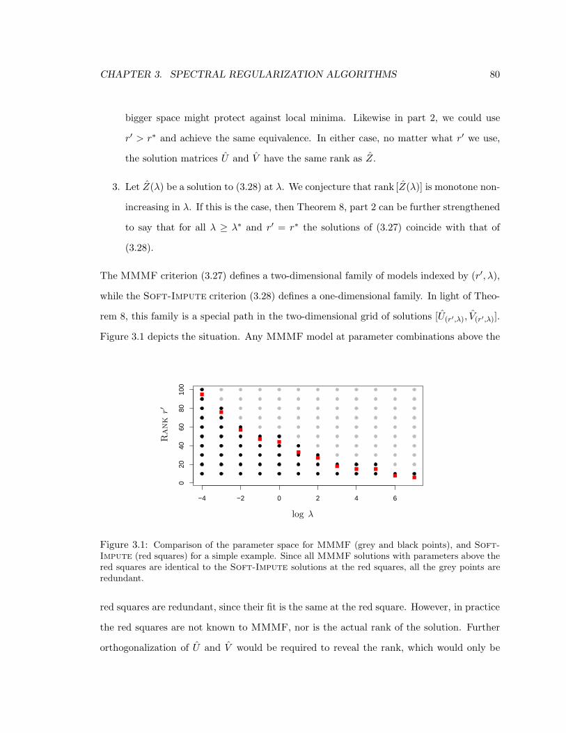
CHAPTER 3. SPECTRAL REGULARIZATION ALGORITHMS 80
bigger space might protect against local minima. Likewise in part 2, we could use
r′ > r∗ and achieve the same equivalence. In either case, no matter what r′ we use,
the solution matrices U and V have the same rank as Z.
3. Let Z(λ) be a solution to (3.28) at λ. We conjecture that rank [Z(λ)] is monotone non-
increasing in λ. If this is the case, then Theorem 8, part 2 can be further strengthened
to say that for all λ ≥ λ∗ and r′ = r∗ the solutions of (3.27) coincide with that of
(3.28).
The MMMF criterion (3.27) defines a two-dimensional family of models indexed by (r′, λ),
while the Soft-Impute criterion (3.28) defines a one-dimensional family. In light of Theo-
rem 8, this family is a special path in the two-dimensional grid of solutions [U(r′,λ), V(r′,λ)].
Figure 3.1 depicts the situation. Any MMMF model at parameter combinations above the
−4 −2 0 2 4 6
020
4060
8010
0
Rank
r′
log λ
Figure 3.1: Comparison of the parameter space for MMMF (grey and black points), and Soft-Impute (red squares) for a simple example. Since all MMMF solutions with parameters above thered squares are identical to the Soft-Impute solutions at the red squares, all the grey points areredundant.
red squares are redundant, since their fit is the same at the red square. However, in practice
the red squares are not known to MMMF, nor is the actual rank of the solution. Further
orthogonalization of U and V would be required to reveal the rank, which would only be

CHAPTER 3. SPECTRAL REGULARIZATION ALGORITHMS 81
approximate (depending on the convergence criterion of the MMMF algorithm).
Despite the equivalence of (3.27) and (3.28) when r′ = min(m,n), the criteria are
quite different. While (3.28) is a convex optimization problem in Z, (3.27) is a non-convex
problem in the variables U, V and has possibly several local minima; see also Abernethy et al.
(2009). It has been observed empirically and theoretically (Burer & Monteiro 2005, Rennie
& Srebro 2005) that bi-convex methods used in the optimization of (3.27) can get stuck in
sub-optimal local minima for a small value of r′ or a poorly chosen starting point. For a
large number of factors r′ and large dimensions m,n the computational cost may be quite
high (See also experimental studies in Section 3.9.2).
Criterion (3.28) is convex in Z for every value of λ, and it outputs the solution Z in the
form of its soft-thresholded SVD, implying that the “factors” U, V are already orthogonal
and the rank is known.
MMMF has two different tuning parameters r′ and λ, both of which are related to
the rank or spectral properties of the matrices U, V . Soft-Impute has only one tuning
parameter λ. The presence of two tuning parameters is problematic:
• It results in a significant increase in computational burden, since for every given value
of r′, one needs to compute an entire system of solutions by varying λ (see Section 3.9
for illustrations).
• In practice when neither the optimal values of r′ and λ are known, a two-dimensional
search (for example, by cross validation) is required to select suitable values.
Further discussions and connections between the tuning parameters and spectral properties
of the matrices can be found in Burer & Monteiro (2005) and Abernethy et al. (2009).
The proof of Theorem 8 requires a lemma.
Lemma 11. For any matrix Z, the following holds:
||Z||∗ = minU,V : Z=UV T
12
(‖U‖2F + ‖V ‖2F
). (3.29)

CHAPTER 3. SPECTRAL REGULARIZATION ALGORITHMS 82
If rank(Z) = k ≤ minm,n, then the minimum above is attained at a factor decomposition
Z = Um×kVTn×k.
Note that in the decomposition Z = UV T in (3.29) there is no constraint on the number
of columns r of the factor matrices Um×r and Vn×r. Lemma 11 is stronger than similar results
appearing in Rennie & Srebro (2005) and Abernethy et al. (2009) which establish (3.29) for
r = minm,n—we give a tighter estimate of the rank k of the underlying matrices. The
proof is given in Appendix 3.A.5.
3.8.1 Proof of Theorem 8
Part 1. For r = min(m,n), any matrix Zm×n can be written in the form of Z = UV T . The
criterion (3.27) can be written as
minU,V
12 ||PΩ(X − UV T )||2F + λ
2 (‖U‖2F + ‖V ‖2F ) (3.30)
= minU,V
12 ||PΩ(X − UV T )||2F + λ‖UV T ‖∗ (by Lemma 11)
= minZ
12 ||PΩ(X − Z)||2F + λ‖Z‖∗. (3.31)
The equivalence of the criteria in (3.30) and (3.31) completes the proof of part 1.
Part 2. Note that if we know that the solution Z∗ to (3.28) with λ = λ∗ has rank r∗, then
Z∗ also solves
minZ, rank(Z)=r∗
12 ||PΩ(X − Z)||2F +λ‖Z‖∗.
We now repeat the steps (3.30)—(3.31), restricting the rank r′ of U and V to be r′ = r∗,
and the result follows.

CHAPTER 3. SPECTRAL REGULARIZATION ALGORITHMS 83
3.9 Numerical Experiments and Comparisons
In this section we study the performance of Soft-Impute, its post-processed variants,
and Hard-Impute for noisy matrix completion problems. The examples assert our claim
that the matrix reconstruction criterion (3.4) (Cai et al. 2010) is too rigid if one seeks
good predictive models. We include the related procedures of Rennie & Srebro (2005) and
Keshavan et al. (2009) in our comparisons.
The reconstruction algorithm OptSpace, described in Keshavan et al. (2009) considers
criterion (3.1) (in the presence of noise). It uses the representation Z = USV ′ (which
need not correspond to the SVD). OptSpace alternates between estimating S and U, V
(in a Grassmann manifold) for computing a rank-r decomposition Z = U SV ′. It starts
with a sparse SVD on a clean version of the observed matrix PΩ(X). This is similar to the
formulation of MMMF (3.27) as detailed in Section 3.8, without the squared Frobenius
norm regularization on the components U, V .
To summarize, we study the following methods:
1. Soft-Impute–Algorithm 2; denoted by SoftImp in the figure labels.
2. Soft-Impute+–post-processing on the output of Soft-Impute, as in Section 3.7;
denoted by SoftImp+ in the figure labels.
3. Hard-Impute–Algorithm 3, starting with the output of Soft-Impute+. We denote
this by HardImp in the figure labels.
4. SVT–algorithm by Cai et al. (2010);
5. OptSpace–reconstruction algorithm by Keshavan et al. (2009);
6. MMMF–algorithm for (3.6) as in Rennie & Srebro (2005).
In all our simulation studies we use the underlying model Zm×n = Um×rV′r×n + ε, where U
and V are random matrices with standard normal Gaussian entries, and ε is i.i.d. Gaussian.

CHAPTER 3. SPECTRAL REGULARIZATION ALGORITHMS 84
Ω is uniformly random over the indices of the matrix with p% percent of missing entries.
These are the models under which the coherence conditions hold true for the matrix com-
pletion problem to be meaningful (Candes & Tao 2009, Keshavan et al. 2009). The signal
to noise ratio for the model and the test-error (standardized) are defined as
SNR =
√var(UV ′)var(ε)
; Test Error =‖P⊥
Ω (UV ′ − Z)‖2F‖P⊥
Ω (UV ′)‖2F.
Training error (standardized) is defined as
Training Error =‖PΩ(Z − Z)‖2F‖PΩ(Z)‖2F
,
the fraction of the error explained on the observed entries by the estimate relative to a zero
estimate.
Figures 3.2, 3.3 and 3.4 show training and test error for all of the algorithms mentioned
above—both as a function of nuclear norm and rank—for the three problem instances.
The results displayed in the figures are averaged over 50 simulations, and also show one-
standard-error bands (hardly visible). In all examples (m,n) = (100, 100). For MMMF
we use r′ = min(m,n) = 100, the number of columns in U and V . The performance of
MMMF is displayed only in the plots with the nuclear norm along the horizontal axis,
since the algorithm does not deliver a precise rank. SNR, true rank and percentage of
missing entries are indicated in the figures. There is a unique correspondence between λ
and nuclear norm. The plots versus rank indicate how effective the nuclear norm is as a
rank approximation—that is whether it recovers the true rank while minimizing prediction
error.
For routines not our own we use the MATLAB code as supplied on webpages by the
authors. For SVT second author of Cai et al. (2010), for OptSpace third author of
Keshavan et al. (2009), and for MMMF first author of Rennie & Srebro (2005).

CHAPTER 3. SPECTRAL REGULARIZATION ALGORITHMS 85
50% missing entries with SNR=1, true rank =10
0 1000 20000.5
0.55
0.6
0.65
0.7
0.75
0.8
0.85
0.9
0.95
1
0 1000 20000
0.1
0.2
0.3
0.4
0.5
0.6
0.7
0.8
0.9
1
Training ErrorTest Error
Nuclear NormNuclear Norm
SoftImp
OptSpaceSVT
MMMF
HardImpSoftImp+
20 40 600.5
0.55
0.6
0.65
0.7
0.75
0.8
0.85
0.9
0.95
1
20 40 600
0.1
0.2
0.3
0.4
0.5
0.6
0.7
0.8
0.9
1
Training ErrorTest Error
RankRank
SoftImp
OptSpaceSVT
HardImpSoftImp+
Figure 3.2: Figure showing training/test error profiles for Soft-Impute+, Soft-Impute, Hard-Impute OptSpace, SVT, MMMF (with full rank 100). Values of test error larger than one arenot shown in the figure. OptSpace is evaluated for ranks ≤ 30.

CHAPTER 3. SPECTRAL REGULARIZATION ALGORITHMS 86
50% missing entries with SNR=1, true rank =6
0 500 1000 15000.3
0.4
0.5
0.6
0.7
0.8
0.9
1
0 500 1000 15000
0.1
0.2
0.3
0.4
0.5
0.6
0.7
0.8
0.9
Training ErrorTest Error
Nuclear NormNuclear Norm
SoftImp
OptSpaceSVT
MMMF
HardImpSoftImp+
20 40 600.3
0.4
0.5
0.6
0.7
0.8
0.9
1
20 40 600
0.1
0.2
0.3
0.4
0.5
0.6
0.7
0.8
0.9
Training ErrorTest Error
RankRank
SoftImp
OptSpaceSVT
HardImpSoftImp+
Figure 3.3: Soft-Impute+ has the best prediction error, closely followed by Soft-Impute andMMMF. Both Hard-Impute and OptSpace have poor prediction error apart from near the truerank. OptSpace is evaluated for a series of ranks ≤ 35. SVT has poor predictiion error with rankof the solution being > 60.

CHAPTER 3. SPECTRAL REGULARIZATION ALGORITHMS 87
80% missing entries with SNR=10, true rank =5
0 200 4000
0.1
0.2
0.3
0.4
0.5
0.6
0.7
0.8
0.9
1
0 200 4000
0.1
0.2
0.3
0.4
0.5
0.6
0.7
0.8
0.9
1
Training ErrorTest Error
Nuclear NormNuclear Norm
SoftImp
OptSpaceSVT
MMMF
HardImpSoftImp+
10 20 300
0.1
0.2
0.3
0.4
0.5
0.6
0.7
0.8
0.9
1
10 20 300
0.1
0.2
0.3
0.4
0.5
0.6
0.7
0.8
0.9
1
Training ErrorTest Error
RankRank
SoftImp
OptSpaceSVT
HardImpSoftImp+
Figure 3.4: With low noise, the performance of Hard-Impute improves and has the best predictionerror, followed by OptSpace. SVT did not converge within 1000 iterations, and the solution seemsto be different from the limiting solution of Soft-Impute

CHAPTER 3. SPECTRAL REGULARIZATION ALGORITHMS 88
3.9.1 Observations
The captions of each of Figures 3.2–3.4 detail the results, which we summarize here. For
the first two figures, the noise is quite high with SNR= 1, and 50% of the entries are miss-
ing. In Figure 3.2 the true rank is 10, while in Figure 3.3 it is 6. Soft-Impute, MMMF
and Soft-Impute+ have the best prediction performance, while Soft-Impute+ is bet-
ter at estimating the correct rank. The other procedures perform poorly here, although
OptSpace improves somewhat in Figure 3.3. SVT has very poor prediction error, sug-
gesting once again that exactly fitting the training data is far too rigid. Soft-Impute+
has the best performance in Figure 3.3 (smaller rank—more aggressive fitting), and Hard-
Impute starts recovering here. In both figures the training error for Soft-Impute (and
hence MMMF) wins as a function of nuclear norm (as it must, by construction), but the
more aggressive fitters Soft-Impute+ and Hard-Impute have better training error as a
function of rank.
Though the nuclear norm is often viewed as a surrogate for the rank of a matrix, we
see in these examples that it can provide a superior mechanism for regularization. This
is similar to the performance of lasso in the context of regression. Although the lasso
penalty can be viewed as a convex surrogate for the ℓ0 penalty in model selection, its ℓ1
penalty provides a smoother and often better basis for regularization.
In Figure 3.4 with SNR= 10 the noise is relatively small compared to the other two
cases. The true underlying rank is 5, but the proportion of missing entries is much higher
at eighty percent. Test errors of both Soft-Impute+ and Soft-Impute are found to
decrease till a large nuclear norm after which they become roughly the same, suggesting no
further impact of regularization. MMMF has slightly better test error than Soft-Impute
around a nuclear norm of 350, while in theory they should be identical. Notice, however,
that the training error is slightly worse (everywhere), suggesting that MMMF is sometimes
trapped in local minima. The fact that this slightly underfit solution does better in test error
CHAPTER 3. SPECTRAL REGULARIZATION ALGORITHMS 89
is a quirk of this particular example. OptSpace performs well in this high-SNR example,
achieving a sharp minima at the true rank of the matrix. Hard-Impute performs the best
in this example. The better performance of bothOptSpace and Hard-Impute over Soft-
Impute can be attributed both to the low-rank truth and the high SNR. This is reminiscent
of the better predictive performance of best-subset or concave penalized regression often
seen over lasso in setups where the underlying model is very sparse (Friedman 2008).
3.9.2 Comparison with Fast MMMF
In this section we compare Soft-Impute with MMMF (Rennie & Srebro 2005) in terms of
computational efficiency. We also examine the consequences of two regularization parame-
ters (r′, λ) for MMMF over one for Soft-Impute.
Rennie & Srebro (2005) describes a fast algorithm based on conjugate-gradient descent
for minimization of the MMMF criterion (3.6). With (3.6) being non-convex, it is hard
to provide theoretical optimality guarantees for the algorithm for arbitrary r′, λ—that is,
what type of solution it converges to or how far it is from the global minimizer.
In Table 3.1 we summarize the performance results of the two algorithms. For both
Soft-Impute and MMMF we consider a equi-spaced grid of 150 λ ∈ [λmin, λmax], with
λmin corresponding to a full-rank solution of Soft-Impute and λmax the zero solution. For
MMMF, three different values of r′ were used, and for each (U , V ) were solved for over
the grid of λ values. A separate held-out validation set with twenty percent of the missing
entries sampled from Ω⊥ were used to train the tuning parameter λ (for each value of r′) for
MMMF and Soft-Impute. Finally we evaluate the standardized prediction errors on a
test set consisting of the remaining eighty percent of the missing entries in Ω⊥. In all cases
we report the training errors and test errors on the optimally tuned λ. Soft-Impute was
run till a tolerance of 10−4 was achieved (fraction of decrease of objective value). Likewise
for MMMF we set the tolerance of the conjugate gradient method to 10−4.

CHAPTER 3. SPECTRAL REGULARIZATION ALGORITHMS 90
Data Method (rank) Test error Training error Time (secs)
(m,n) = (102, 102) Soft-Impute (39) 0.7238 (0.0027) 0.0720 4.1745|Ω| = 5× 10³(50%) MMMF (20) 0.7318 (0.0031) 0.2875 48.1090SNR= 3 MMMF (60) 0.7236 (0.0027) 0.1730 62.0230rank (R)= 30 MMMF (100) 0.7237 (0.0027) 0.1784 96.2750
(m,n) = (102, 102) Soft-Impute (37) 0.5877 (0.0047) 0.0017 4.0976|Ω| = 2× 10³(20%) MMMF (20) 0.5807 (0.0049) 0.0186 53.7533SNR= 10 MMMF (60) 0.5823 (0.0049) 0.0197 62.0230rank(R)= 10 MMMF (100) 0.5823 (0.0049) 0.0197 84.0375
(m,n) = (102, 102) Soft-Impute (59) 0.6008 (0.0028) 0.0086 3.8447|Ω| = 8× 10³(80%) MMMF (20) 0.6880 (0.0029) 0.4037 33.8685SNR= 10 MMMF (60) 0.5999 (0.0028) 0.0275 57.3488rank(R)= 45 MMMF (100) 0.5999 (0.0028) 0.0275 89.4525
Table 3.1: Performances of Soft-Impute and MMMF for different problem instances, in termsof test error (with standard errors in parentheses), training error and times for learning the models.Soft-Impute,“rank” denotes the rank of the recovered matrix, at the optimally chosen value ofλ. For the MMMF, “rank” indicates the value of r′ in Um×r′, Vn×r′ . Results are averaged over 50simulations.
In Table 3.1, for every algorithm total time indicates the time required for evaluating so-
lutions over the entire grid of λ values. In these examples, we used direct SVD factorization
based methods for the SVD computation, since the size of the problems were quite small.
In all these examples we observe that Soft-Impute performs very favorably in terms of
total times. For MMMF the time to train the models increase with increasing rank r′; and
in case the underlying matrix has rank which is larger than r′, the computational cost will
be large in order to get competitive predictive accuracy. This point is supported in the
examples of Table 3.1. It is important to note that, the prediction error of Soft-Impute
as obtained on the validation set is actually within standard error of the best prediction
error produced by all the MMMF models.
In addition we also performed some medium-scale examples increasing the dimensions of the
matrices. To make comparisons fair, Soft-Impute made use of direct SVD computations
(in MATLAB) instead of iterative algorithms exploiting the specialized Sparse+Low-Rank

CHAPTER 3. SPECTRAL REGULARIZATION ALGORITHMS 91
structure (3.22). We report our findings on one such simulation example:
• For (m,n) = (2000, 1000), |Ω|/(m ·n) = 0.2, rank = 500 and SNR=10; Soft-Impute
takes 1.29 hours to compute solutions on a grid of 100 λ values. The test error on the
validation set and training error are 0.9630 and 0.4375 with the recovered solution
having a rank of 225.
For the same problem, MMMF with r′ = 200 takes 6.67 hours returning a solution
with test-error 0.9678 and training error 0.6624. With r′ = 400 it takes 12.89 hrs with
test and training errors 0.9659 and 0.6564 respectively.
We will like to note that DeCoste (2006) proposed an efficient implementation of MMMF
via an ensemble based approach, which is quite different in spirit from the batch optimization
algorithms we are studying in this paper. Hence we do not compare it with soft-impute.
3.9.3 Comparison with Nesterov’s Accelerated Gradient Method
Ji & Ye (2009) proposed a first-order algorithm based on Nesterov’s acceleration scheme
(Nesterov 2007), for nuclear norm minimization for a generic multi-task learning problem
(Argyriou et al. 2008, Argyriou et al. 2007). Their algorithm (Liu et al. 2009, Ji & Ye 2009)
can be adapted to the Soft-Impute problem (3.10); hereafter we refer to it as Nesterov.
It requires one to compute the SVD of a dense matrix having the dimensions of X, which
makes it prohibitive for large-scale problems. We instead would make use of the structure
(3.22) for the SVD computation, a special characteristic of matrix completion which is
not present in a generic multi-task learning problem. Here we compare the performances of
Soft-Impute and Nesterov on small scale examples, where direct SVDs can be computed
easily.
Since both algorithms solve the same criterion, the quality of the solutions—objective
values, training and test errors—will be the same (within tolerance). We hence compare
their performances based on the times taken by the algorithms to converge to the optimal

CHAPTER 3. SPECTRAL REGULARIZATION ALGORITHMS 92
solution of (3.10) on a grid of values of λ. Both algorithms compute a path of solutions
using warm starts. Results are shown in Figure 3.5, for four different scenarios described
in Table 3.2.
Example (m,n) |Ω|/(m · n) Rank Test Error
i (100, 100) 0.5 5 0.4757ii (100, 100) 0.2 5 0.0668iii (100, 100) 0.8 5 0.0022iv (1000, 500) 0.5 30 0.0028
Table 3.2: Four different examples used for timing comparisons of Soft-Impute and (accelerated)Nesterov. In all cases the SNR= 10.
Figure 3.5 shows the time to convergence for the two algorithms. Their respective
number of iterations are not comparable. This is because Nesterov uses a line-search
to compute an adaptive step-size (approximate the Lipschitz constant) at every iteration,
whereas Soft-Impute does not.
Soft-Impute has a rate of convergence given by Theorem 7, which for large k is worse
than the accelerated version Nesterov with rate O(1/k2). However, timing comparisons
in Figure 3.5 show that soft-impute performs very favorably. We do not know the exact
reason behind this, but mention some possibilities. Firstly the rates are worst case conver-
gence rates. On particular problem instances of the form (3.10), the rates of convergence in
practice of soft-impute and Nesterov may be quite similar. Since Ji & Ye (2009) uses an
adaptive step-size strategy, the choice of a step-size may be time consuming. soft-impute
on the other hand, uses a constant step size.
Additionally, it appears that the use of the momentum term in Nesterov affects the
Sparse+Low-rank decomposition (3.22). This may prevent the algorithm to be adapted for
solving large problems, due to costly SVD computations.

CHAPTER 3. SPECTRAL REGULARIZATION ALGORITHMS 93
0 0.2 0.4 0.60
0.5
1
1.5
2
2.5
3
Soft−ImputeNesterov
Tim
e(insecs)
i
0 0.2 0.4 0.60
0.5
1
1.5
2
2.5
3ii
0.1 0.2 0.3 0.4 0.5 0.60
0.5
1
1.5
2
2.5
3
Tim
e(insecs)
iii
log(‖Zλ‖∗/C + 1)0.45 0.5 0.55 0.6 0.65 0.7
0
20
40
60
80
100
120iv
log(‖Zλ‖∗/C + 1)
Figure 3.5: Timing comparisons of Soft-Impute and (accelerated) Nesterov over a grid of λvalues for examples i–iv. The horizontal axis corresponds to the standardized nuclear norm, withC = maxλ ‖Zλ‖∗. Results are averaged over 10 simulations.
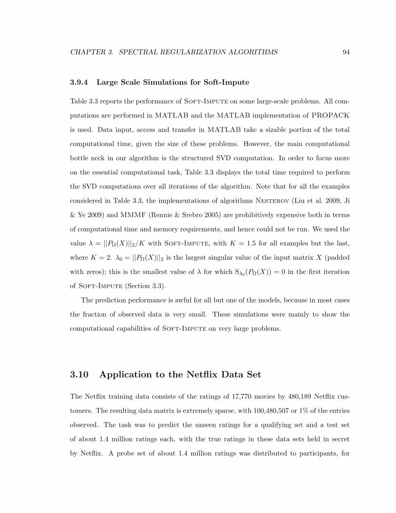
CHAPTER 3. SPECTRAL REGULARIZATION ALGORITHMS 94
3.9.4 Large Scale Simulations for Soft-Impute
Table 3.3 reports the performance of Soft-Impute on some large-scale problems. All com-
putations are performed in MATLAB and the MATLAB implementation of PROPACK
is used. Data input, access and transfer in MATLAB take a sizable portion of the total
computational time, given the size of these problems. However, the main computational
bottle neck in our algorithm is the structured SVD computation. In order to focus more
on the essential computational task, Table 3.3 displays the total time required to perform
the SVD computations over all iterations of the algorithm. Note that for all the examples
considered in Table 3.3, the implementations of algorithms Nesterov (Liu et al. 2009, Ji
& Ye 2009) and MMMF (Rennie & Srebro 2005) are prohibitively expensive both in terms
of computational time and memory requirements, and hence could not be run. We used the
value λ = ||PΩ(X)||2/K with Soft-Impute, with K = 1.5 for all examples but the last,
where K = 2. λ0 = ||PΩ(X)||2 is the largest singular value of the input matrix X (padded
with zeros); this is the smallest value of λ for which Sλ0(PΩ(X)) = 0 in the first iteration
of Soft-Impute (Section 3.3).
The prediction performance is awful for all but one of the models, because in most cases
the fraction of observed data is very small. These simulations were mainly to show the
computational capabilities of Soft-Impute on very large problems.
3.10 Application to the Netflix Data Set
The Netflix training data consists of the ratings of 17,770 movies by 480,189 Netflix cus-
tomers. The resulting data matrix is extremely sparse, with 100,480,507 or 1% of the entries
observed. The task was to predict the unseen ratings for a qualifying set and a test set
of about 1.4 million ratings each, with the true ratings in these data sets held in secret
by Netflix. A probe set of about 1.4 million ratings was distributed to participants, for
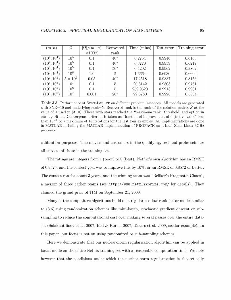
CHAPTER 3. SPECTRAL REGULARIZATION ALGORITHMS 95
(m,n) |Ω| |Ω|/(m · n) Recovered Time (mins) Test error Training error×100% rank
(104, 104) 105 0.1 40∗ 0.2754 0.9946 0.6160(104, 104) 105 0.1 40∗ 0.3770 0.9959 0.6217(104, 104) 105 0.1 50∗ 0.4292 0.9962 0.3862(104, 104) 106 1.0 5 1.6664 0.6930 0.6600(105, 105) 5× 10⁶ 0.05 40∗ 17.2518 0.9887 0.8156(105, 105) 107 0.1 5 20.3142 0.9803 0.9761(106, 105) 108 0.1 5 259.9620 0.9913 0.9901(106, 106) 107 0.001 20∗ 99.6780 0.9998 0.5834
Table 3.3: Performance of Soft-Impute on different problem instances. All models are generatedwith SNR=10 and underlying rank=5. Recovered rank is the rank of the solution matrix Z at thevalue of λ used in (3.10). Those with stars reached the “maximum rank” threshold, and option inour algorithm. Convergence criterion is taken as “fraction of improvement of objective value” lessthan 10−4 or a maximum of 15 iterations for the last four examples. All implementations are donein MATLAB including the MATLAB implementation of PROPACK on a Intel Xeon Linux 3GHzprocessor.
calibration purposes. The movies and customers in the qualifying, test and probe sets are
all subsets of those in the training set.
The ratings are integers from 1 (poor) to 5 (best). Netflix’s own algorithm has an RMSE
of 0.9525, and the contest goal was to improve this by 10%, or an RMSE of 0.8572 or better.
The contest ran for about 3 years, and the winning team was “Bellkor’s Pragmatic Chaos”,
a merger of three earlier teams (see http://www.netflixprize.com/ for details). They
claimed the grand prize of $1M on September 21, 2009.
Many of the competitive algorithms build on a regularized low-rank factor model similar
to (3.6) using randomization schemes like mini-batch, stochastic gradient descent or sub-
sampling to reduce the computational cost over making several passes over the entire data-
set (Salakhutdinov et al. 2007, Bell & Koren. 2007, Takacs et al. 2009, see,for example). In
this paper, our focus is not on using randomized or sub-sampling schemes.
Here we demonstrate that our nuclear-norm regularization algorithm can be applied in
batch mode on the entire Netflix training set with a reasonable computation time. We note
however that the conditions under which the nuclear-norm regularization is theoretically

CHAPTER 3. SPECTRAL REGULARIZATION ALGORITHMS 96
λ Rank Time (hrs) RMSE
λ0/250 42 1.36 0.9622λ0/300 66 2.21 0.9572λ0/500 81 2.83 0.9543λ0/600 95 3.27 0.9497
Table 3.4: Results of applying Soft-Impute to the Netflix data. λ0 = ||PΩ(X)||2; see Section 3.9.4.The computations were done on a Intel Xeon Linux 3GHz processor; timings are reported based onMATLAB implementations of PROPACK and our algorithm. RMSE is root-mean squared error, asdefined in the text.
meaningful (Candes & Tao 2009, Srebro, Alon & Jaakkola 2005) are not met on the Netflix
data set.
We applied Soft-Impute to the training data matrix and then performed a least-
squares unshrinking on the singular values with the singular vectors and the training data
row and column means as the bases. The latter was performed on a data-set of size 105
randomly drawn from the probe set. The prediction error (RMSE) is obtained on a left out
portion of the probe set. Table 3.4 reports the performance of the procedure for different
choices of the tuning parameter λ (and the corresponding rank); times indicate the total
time taken for the SVD computations over all iterations. A maximum of 10 iterations were
performed for each of the examples. Again, these results are not competitive with those of
the competition leaders, but rather demonstrate the feasibility of applying Soft-Impute
to such a large data set.
3.A Appendix to Chapter 3
We begin with the proof of Lemma 6.

CHAPTER 3. SPECTRAL REGULARIZATION ALGORITHMS 97
3.A.1 Proof of Lemma 6
Proof. Let Z = Um×nDn×nV′n×n be the SVD of Z. Assume without loss of generality, m ≥ n.
We will explicitly evaluate the closed form solution of the problem (3.8). Note that
12‖Z −W‖2F + λ‖Z‖∗ = 1
2
‖W‖2F − 2
n∑
i=1
diu′iWvi +
n∑
i=1
d2i
+ λ
n∑
i=1
di (3.32)
where
D = diag[d1, . . . , dn
], U = [u1, . . . , un] , V = [v1, . . . , vn] .
Minimizing (3.32) is equivalent to minimizing
−2
n∑
i=1
diu′iWvi +
n∑
i=1
d2i +
n∑
i=1
2λdi; w.r.t. (ui, vi, di), i = 1, . . . , n,
under the constraints U ′U = In, V′V = In and di ≥ 0 ∀i.
Observe the above is equivalent to minimizing (w.r.t. U , V ) the function Q(U , V ):
Q(U , V ) = minD≥0
12
−2
n∑
i=1
diu′iWvi +
n∑
i=1
d2i
+ λ
n∑
i=1
di. (3.33)
Since the objective (3.33) to be minimized w.r.t. D, is separable in di, i = 1, . . . , n; it suffices
to minimize it w.r.t. each di separately.
The problem
minimizedi≥0
12
−2diu
′iWvi + d2i
+ λdi (3.34)
can be solved looking at the stationary conditions of the function using its sub-gradient
(Nesterov 2003). The solution of the above problem is given by Sλ(u′iWvi) = (u′iWvi−λ)+,
the soft-thresholding of u′iWvi (without loss of generality, we can take u′iWvi to be non-
negative). More generally the soft-thresholding operator (Friedman, Hastie, Hoefling &

CHAPTER 3. SPECTRAL REGULARIZATION ALGORITHMS 98
Tibshirani 2007, Hastie et al. 2009) is given by Sλ(x) = sgn(x)(|x| − λ)+. See Fried-
man, Hastie, Hoefling & Tibshirani (2007) for more elaborate discussions on how the
soft-thresholding operator arises in univariate penalized least-squares problems with the
ℓ1 penalization.
Plugging the values of optimal di, i = 1, . . . , n; obtained from (3.34) in (3.33) we get
Q(U , V ) = 12
‖W‖2F − 2
n∑
i=1
(u′iWvi − λ)+(u′iWvi − λ) + (u′iXvi − λ)2+
. (3.35)
Minimizing Q(U , V ) w.r.t. (U , V ) is equivalent to maximizing
n∑
i=1
2(u′iWvi − λ)+(u
′iWvi − λ)− (u′iWvi − λ)2+
=
∑
u′
iWvi>λ
(u′iWvi − λ)2. (3.36)
It is a standard fact that for every i the problem
maximize‖u‖2
2≤1,‖v‖2
2≤1
u′Wv; such that u ⊥ u1, . . . , ui−1, v ⊥ v1, . . . , vi−1
is solved by ui, vi, the left and right singular vectors of the matrix W corresponding to
its ith largest singular value. The maximum value equals the singular value. It is easy
to see that maximizing the expression to the right of (3.36) wrt (ui, vi), i = 1, . . . , n is
equivalent to maximizing the individual terms u′iWvi. If r(λ) denotes the number of singular
values of W larger than λ then the (ui, vi) , i = 1, . . . that maximize the expression (3.36)
correspond to[u1, . . . , ur(λ)
]and
[v1, . . . , vr(λ)
]; the r(λ) left and right singular vectors ofW
corresponding to the largest singular values. From (3.34) the optimal D = diag[d1, . . . , dn
]
is given by Dλ = diag [(d1 − λ)+, . . . , (dn − λ)+] .
Since the rank of W is r, the minimizer Z of (3.8) is given by UDλV′ as in (3.9).
Remark 1. For a more general spectral regularization of the form λ∑
i p(γi(Z)) (as com-
pared to∑
i λγi(Z) used above) the optimization problem (3.34) will be modified accordingly.
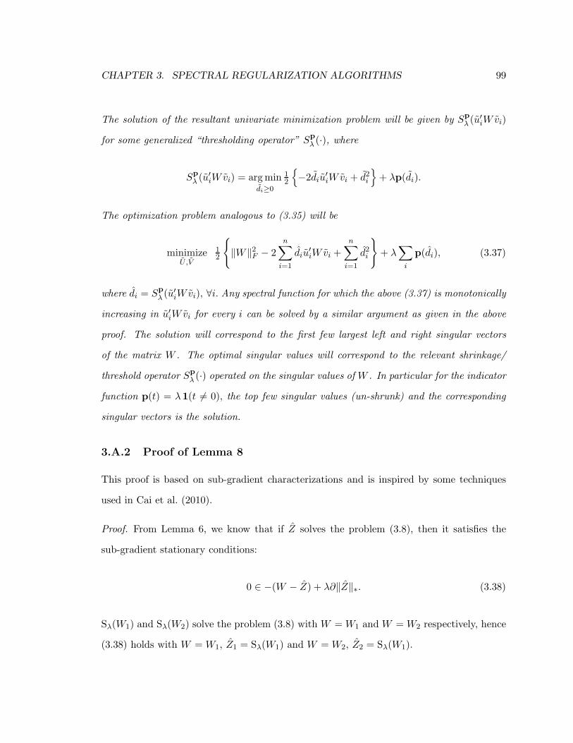
CHAPTER 3. SPECTRAL REGULARIZATION ALGORITHMS 99
The solution of the resultant univariate minimization problem will be given by Spλ (u
′iWvi)
for some generalized “thresholding operator” Spλ (·), where
Spλ (u
′iWvi) = argmin
di≥0
12
−2diu
′iWvi + d2i
+ λp(di).
The optimization problem analogous to (3.35) will be
minimizeU ,V
12
‖W‖2F − 2
n∑
i=1
diu′iWvi +
n∑
i=1
d2i
+ λ
∑
i
p(di), (3.37)
where di = Spλ (u
′iWvi), ∀i. Any spectral function for which the above (3.37) is monotonically
increasing in u′iWvi for every i can be solved by a similar argument as given in the above
proof. The solution will correspond to the first few largest left and right singular vectors
of the matrix W . The optimal singular values will correspond to the relevant shrinkage/
threshold operator Spλ (·) operated on the singular values of W . In particular for the indicator
function p(t) = λ1(t 6= 0), the top few singular values (un-shrunk) and the corresponding
singular vectors is the solution.
3.A.2 Proof of Lemma 8
This proof is based on sub-gradient characterizations and is inspired by some techniques
used in Cai et al. (2010).
Proof. From Lemma 6, we know that if Z solves the problem (3.8), then it satisfies the
sub-gradient stationary conditions:
0 ∈ −(W − Z) + λ∂‖Z‖∗. (3.38)
Sλ(W1) and Sλ(W2) solve the problem (3.8) with W = W1 and W = W2 respectively, hence
(3.38) holds with W = W1, Z1 = Sλ(W1) and W = W2, Z2 = Sλ(W1).

CHAPTER 3. SPECTRAL REGULARIZATION ALGORITHMS 100
The sub-gradients of the nuclear norm ‖Z‖∗ are given by
∂‖Z‖∗ = UV ′ + ω : ωm×n, U′ω = 0, ωV = 0, ‖ω‖2 ≤ 1, (3.39)
where Z = UDV ′ is the SVD of Z.
Let p(Zi) denote an element in ∂‖Zi‖∗. Then
Zi −Wi + λp(Zi) = 0, i = 1, 2.
The above gives
(Z1 − Z2)− (W1 −W2) + λ(p(Z1)− p(Z2)) = 0, (3.40)
from which we obtain
〈Z1 − Z2, Z1 − Z2〉 − 〈W1 −W2, Z1 − Z2〉+ λ〈p(Z1)− p(Z2), Z1 − Z2〉 = 0,
where 〈a, b〉 = trace(a′b).
Now observe that
〈p(Z1)− p(Z2), Z1 − Z2〉 = 〈p(Z1), Z1〉 − 〈p(Z1), Z2〉 − 〈p(Z2), Z1〉+ 〈p(Z2), Z2〉. (3.41)
By the characterization of subgradients as in (3.39), we have
〈p(Zi), Zi〉 = ‖Zi‖∗ and ‖p(Zi)‖2 ≤ 1, i = 1, 2.
This implies
|〈p(Zi), Zj〉| ≤ ‖p(Zi)‖2‖Zj‖∗ ≤ ‖Zj‖∗ for i 6= j ∈ 1, 2.

CHAPTER 3. SPECTRAL REGULARIZATION ALGORITHMS 101
Using the above inequalities in (3.41) we obtain:
〈p(Z1), Z1〉+ 〈p(Z2), Z2〉 = ‖Z1‖∗ + ‖Z2‖∗ (3.42)
−〈p(Z1), Z2〉 − 〈p(Z2), Z1〉 ≥ −‖Z2‖∗ − ‖Z1‖∗. (3.43)
Using (3.42,3.43) we see that the r.h.s. of (3.41) is non-negative. Hence
〈p(Z1)− p(Z2), Z1 − Z2〉 ≥ 0.
Using the above in (3.40), we obtain:
‖Z1 − Z2‖2F = 〈Z1 − Z2, Z1 − Z2〉 ≤ 〈W1 −W2, Z1 − Z2〉. (3.44)
Using the Cauchy-Schwarz Inequality, ‖Z1 − Z2‖F ‖W1 −W2‖F ≥ 〈Z1 − Z2,W1 −W2〉
in (3.44) we get
‖Z1 − Z2‖2F ≤ 〈Z1 − Z2,W1 −W2〉 ≤ ‖Z1 − Z2‖F ‖W1 −W2‖F
and in particular
‖Z1 − Z2‖2F ≤ ‖Z1 − Z2‖F ‖W1 −W2‖F .
The above further simplifies to
‖W1 −W2‖2F ≥ ‖Z1 − Z2‖
2F = ‖Sλ(W1)− Sλ(W2)‖
2F .

CHAPTER 3. SPECTRAL REGULARIZATION ALGORITHMS 102
3.A.3 Proof of Lemma 9
Proof. We will first show (3.15) by observing the following inequalities:
‖Zk+1λ − Zk
λ‖2F = ‖Sλ(PΩ(X) + P⊥
Ω (Zkλ))− Sλ(PΩ(X) + P⊥
Ω (Zk−1λ ))‖2F
(by Lemma 8) ≤ ‖(PΩ(X) + P⊥
Ω (Zkλ))−(PΩ(X) + P⊥
Ω (Zk−1λ )
)‖2F
= ‖P⊥Ω (Zk
λ − Zk−1λ )‖2F (3.45)
≤ ‖Zkλ − Zk−1
λ ‖2F . (3.46)
The above implies that the sequence ‖Zkλ − Zk−1
λ ‖2F converges (since it is decreasing and
bounded below). We still require to show that ‖Zkλ − Zk−1
λ ‖2F converges to zero.
The convergence of ‖Zkλ − Zk−1
λ ‖2F implies that:
‖Zk+1λ − Zk
λ‖2F − ‖Z
kλ − Zk−1
λ ‖2F → 0 as k →∞.
The above observation along with the inequality in (3.45,3.46) gives
‖P⊥Ω (Zk
λ − Zk−1λ )‖2F − ‖Z
kλ − Zk−1
λ ‖2F → 0 =⇒ PΩ(Zkλ − Zk−1
λ )→ 0, (3.47)
as k →∞.
Lemma 7 shows that the non-negative sequence fλ(Zkλ) is decreasing in k. So as k →∞
the sequence fλ(Zkλ) converges.
Furthermore from (3.13,3.14) we have
Qλ(Zk+1λ |Zk
λ)−Qλ(Zk+1λ |Zk+1
λ )→ 0 as k →∞,
which implies that
‖P⊥Ω (Zk
λ)− P⊥Ω (Zk+1
λ )‖2F → 0 as k →∞.

CHAPTER 3. SPECTRAL REGULARIZATION ALGORITHMS 103
The above along with (3.47) gives
Zkλ − Zk−1
λ → 0 as k →∞.
This completes the proof.
3.A.4 Proof of Lemma 10
Proof. The sub-gradients of the nuclear norm ‖Z‖∗ are given by
∂‖Z‖∗ = UV ′ +W : Wm×n, U′W = 0, WV = 0, ‖W‖2 ≤ 1, (3.48)
where Z = UDV ′ is the SVD of Z. Since Zkλ minimizes Qλ(Z|Z
k−1λ ), it satisfies:
0 ∈ −(PΩ(X) + P⊥Ω (Zk−1
λ )− Zkλ) + ∂‖Zk
λ‖∗ ∀k. (3.49)
Suppose Z∗ is a limit point of the sequence Zkλ . Then there exists a subsequence nk ⊂
1, 2, . . . such that Znk
λ → Z∗ as k →∞.
By Lemma 9 this subsequence Znk
λ satisfies
Znk
λ − Znk−1λ → 0
implying
P⊥Ω (Znk−1
λ )− Znk
λ −→ P⊥Ω (Z∗
λ)− Z∗λ = −PΩ(Z
∗).
Hence,
(PΩ(X) + P⊥Ω (Znk−1
λ )− Znk
λ ) −→ (PΩ(X)− PΩ(Z∗λ)). (3.50)
For every k, a sub-gradient p(Zkλ) ∈ ∂‖Zk
λ‖∗ corresponds to a tuple (uk, vk, wk) satisfying

CHAPTER 3. SPECTRAL REGULARIZATION ALGORITHMS 104
the properties of the set ∂‖Zkλ‖∗ (3.48).
Consider p(Znk
λ ) along the sub-sequence nk. As nk −→∞, Znk
λ −→ Z∗λ.
Let
Znk
λ = unkDnk
v′nk, Z∗ = u∞D∗v′∞
denote the SVD’s. The product of the singular vectors converge u′nkvnk→ u′∞v∞. Further-
more due to boundedness (passing on to a further subsequence if necessary) wnk→ w∞.
The limit u∞v′∞ + w∞ clearly satisfies the criterion of being a sub-gradient of Z∗. Hence
this limit corresponds to p(Z∗λ) ∈ ∂‖Z∗
λ‖∗.
Furthermore from (3.49, 3.50), passing on to the limits along the subsequence nk, we
have
0 ∈ −(PΩ(X) − PΩ(Z∗λ)) + ∂‖Z∗
λ‖∗.
Hence the limit point Z∗λ is a stationary point of fλ(Z).
We shall now prove (3.16). We know that for every nk
Znk
λ = Sλ(PΩ(X) + P⊥Ω (Znk−1
λ )). (3.51)
From Lemma 9, we know Znk
λ − Znk−1λ → 0. This observation along with the continuity of
Sλ(·) gives
Sλ(PΩ(X) + P⊥Ω (Znk−1
λ ))→ Sλ(PΩ(X) + P⊥Ω (Z∗
λ)).
Thus passing over to the limits on both sides of (3.51) we get
Z∗λ = Sλ(PΩ(X) + P⊥
Ω (Z∗λ)),
therefore completing the proof.

CHAPTER 3. SPECTRAL REGULARIZATION ALGORITHMS 105
3.A.5 Proof of Lemma 11
The proof is motivated by the principle of embedding an arbitrary matrix into a positive
semidefinite matrix (Fazel 2002). We require the following proposition, which we prove
using techniques used in the same reference.
Proposition 1. Suppose matrices Wm×m, Wn×n, Zm×n satisfy the following:
W Z
ZT W
0.
Then trace(W ) + trace(W ) ≥ 2‖Z‖∗.
Proof. Let Zm×n = Lm×rΣr×rRTn×r denote the SVD of Z, where r is the rank of the matrix
Z. Observe that the trace of the product of two positive semidefinite matrices is always
non-negative. Hence we have the following inequality:
trace
LLT −LRT
−RLT RRT
W Z
ZT W
0.
Simplifying the above expression we get:
trace(LLTW )− trace(LRTZT )− trace(RLTZ) + trace(RRT W ) ≥ 0. (3.52)
Due to the orthogonality of the columns of L,R we have the following inequalities:
trace(LLTW ) ≤ trace(W ) and trace(RRT W ) ≤ trace(W ).
Furthermore, using the SVD of Z:
trace(LRTZT ) = trace(Σ) = trace(LRTZT ).

CHAPTER 3. SPECTRAL REGULARIZATION ALGORITHMS 106
Using the above in (3.52), we have:
trace(W ) + trace(W ) ≥ 2 trace(Σ) = 2 ‖Z‖∗.
Proof of Lemma 11. For the matrix Z, consider any decomposition of the form Z = Um×rVTn×r
and construct the following matrix
U UT Z
ZT V V T
=
U
V
(UT V T ), (3.53)
which is positive semidefinite. Applying Proposition 1 to the left hand matrix in (3.53), we
have:
trace(U UT ) + trace(V V T ) ≥ 2 ‖Z‖∗.
Minimizing both sides above w.r.t. the decompositions Z = Um×rVTn×r; we have
minU ,V ; Z=UV T
trace(U UT ) + trace(V V T )
≥ 2 ‖Z‖∗. (3.54)
Through the SVD of Z we now show that equality is attained in (3.54). Suppose Z is of rank
k ≤ min(m,n), and denote its SVD by Zm×n = Lm×kΣk×kRTn×k. Then for U = Lm×kΣ
12k×k
and V = Rn×kΣ12k×k the equality in (3.54) is attained.
Hence, we have:
‖Z‖∗ = minU ,V ;Z=UV T
trace(U UT ) + trace(V V T )
= minU ,V ;Z=Um×kV
Tn×k
trace(U UT ) + trace(V V T )
.
Note that the minimum can also be attained for matrices with r ≥ k or even r ≥ min(m,n);
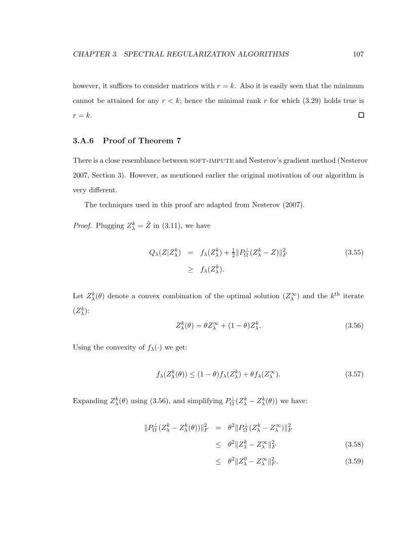
CHAPTER 3. SPECTRAL REGULARIZATION ALGORITHMS 107
however, it suffices to consider matrices with r = k. Also it is easily seen that the minimum
cannot be attained for any r < k; hence the minimal rank r for which (3.29) holds true is
r = k.
3.A.6 Proof of Theorem 7
There is a close resemblance between soft-impute and Nesterov’s gradient method (Nesterov
2007, Section 3). However, as mentioned earlier the original motivation of our algorithm is
very different.
The techniques used in this proof are adapted from Nesterov (2007).
Proof. Plugging Zkλ = Z in (3.11), we have
Qλ(Z|Zkλ) = fλ(Z
kλ) +
12‖P
⊥Ω (Zk
λ − Z)‖2F (3.55)
≥ fλ(Zkλ).
Let Zkλ(θ) denote a convex combination of the optimal solution (Z∞
λ ) and the kth iterate
(Zkλ):
Zkλ(θ) = θZ∞
λ + (1− θ)Zkλ . (3.56)
Using the convexity of fλ(·) we get:
fλ(Zkλ(θ)) ≤ (1− θ)fλ(Z
kλ) + θfλ(Z
∞λ ). (3.57)
Expanding Zkλ(θ) using (3.56), and simplifying P⊥
Ω (Zkλ − Zk
λ(θ)) we have:
‖P⊥Ω (Zk
λ − Zkλ(θ))‖
2F = θ2‖P⊥
Ω (Zkλ − Z∞
λ )‖2F
≤ θ2‖Zkλ − Z∞
λ ‖2F (3.58)
≤ θ2‖Z0λ − Z∞
λ ‖2F . (3.59)

CHAPTER 3. SPECTRAL REGULARIZATION ALGORITHMS 108
Line 3.59 follows from (3.58) by observing that ‖Zmλ − Z∞
λ ‖2F ≤ ‖Z
m−1λ − Z∞
λ ‖2F , ∀m—a
consequence of the inequalities (3.19) and (3.18), established in Theorem 6.
Using (3.55), the value of fλ(Z) at the (k + 1)th iterate satisfies the following chain of
inequalities:
fλ(Zk+1λ ) ≤ min
Z
fλ(Z) + 1
2‖P⊥Ω (Zk
λ − Z)‖2F
≤ minθ∈[0,1]
fλ(Z
kλ(θ)) +
12‖P
⊥Ω (Zk
λ − Zkλ(θ))‖
2F
(3.60)
≤ minθ∈[0,1]
fλ(Z
kλ) + θ(fλ(Z
∞λ )− fλ(Z
kλ)) +
12θ
2‖Z0λ − Z∞
λ ‖2F
. (3.61)
Line 3.61 follows from Line 3.60, by using (3.57) and (3.59).
The r.h.s. expression in (3.61), is minimized at θ(k + 1) given by
θ(k + 1) = min1, θk ∈ [0, 1], where,
θk =fλ(Z
kλ)− fλ(Z
∞λ )
‖Z0λ − Z∞
λ ‖2F
.
If ‖Z0λ − Z∞
λ ‖2F = 0, then we take θk =∞.
Note that θk is a decreasing sequence. This implies that if θk0 ≤ 1 then θm ≤ 1 for all
m ≥ k0.
Suppose, θ0 > 1. Then θ(1) = 1. Hence using (3.61) we have:
fλ(Z1λ)− fλ(Z
∞λ ) ≤ 1
2‖Z0λ − Z∞
λ ‖2F =⇒ θ1 ≤
12 .
Thus we get back to the former case.
Hence θk ≤ 1 for all k ≥ 1.
In addition, observe the previous deductions show that, if θ0 > 1 then (3.20) holds true
for k = 1.
Combining the above observations, plugging in the value of θ in (3.61) and simplifying,

CHAPTER 3. SPECTRAL REGULARIZATION ALGORITHMS 109
we get:
fλ(Zk+1λ )− fλ(Z
kλ) ≤ −
(fλ(Zkλ)− fλ(Z
∞λ ))2
2‖Z0λ − Z∞
λ ‖2F
. (3.62)
For the sake of notational convenience, we define the sequence αk = fλ(Zkλ)− fλ(Z
∞λ ). It is
easily seen that αk is a non-negative decreasing sequence.
Using this notation in (3.62) we get:
αk ≥α2k
2‖Z0λ − Z∞
λ ‖2F
+ αk+1
(Since αk ↓) ≥αkαk+1
2‖Z0λ − Z∞
λ ‖2F
+ αk+1. (3.63)
Dividing both sides of the inequality in (3.63), by αkαk+1 we have:
α−1k+1 ≥
1
2‖Z0λ − Z∞
λ ‖2F
+ α−1k . (3.64)
Summing both sides of (3.64) over 1 ≤ k ≤ (k − 1) we get:
α−1k ≥
k − 1
2‖Z0λ − Z∞
λ ‖2F
+ α−11 . (3.65)
Since θ1 ≤ 1, we observe α1/(2‖Z0λ − Z∞
λ ‖2F ) ≤ 1/2—using this in (3.65) and rearranging
terms we get, the desired inequality (3.20)—completing the proof of the Theorem.

Part III
Covariance Selection & Graphical
Lasso : New Insights &
Alternatives
110

111
This part of the thesis is dedicated to studying properties of the ℓ1 penalized negative
log-likelihood for learning undirected Gaussian graphical models, popularly dubbed as the
Graphical Lasso (Friedman, Hastie & Tibshirani 2007, Banerjee et al. 2008) or glasso . It
is divided into two chapters:
Chapter 4: Exact Covariance Thresholding for glasso :
This is about a previously unknown and interesting property of glasso which es-
tablishes the equivalence between the connected components of the sparse precision
graph and the same of a thresholded version of the sample covariance matrix.
Chapter 5: glasso New Insights and Alternatives :
This chapter highlights some of the properties of the glasso algorithm that appear
mysterious and providing explanations to them. In the process of our analysis, we
propose new and superior algorithm(s) on the primal : p-glasso and dp-glasso and
justify their usefulness.

Chapter 4
Exact Covariance Thresholding for
glasso
Abstract: We consider the sparse inverse covariance regularization problem or graphical lasso with
regularization parameter λ. Suppose the sample covariance graph formed by thresholding the entries
of the sample covariance matrix at λ is decomposed into connected components. We show that the
vertex-partition induced by the connected components of the thresholded sample covariance graph
(at λ) is exactly equal to that induced by the connected components of the estimated concentration
graph, obtained by solving the graphical lasso problem for the same λ. This characterizes a very
interesting property of a path of graphical lasso solutions. Furthermore, this simple rule, when used
as a wrapper around existing algorithms for the graphical lasso, leads to enormous performance
gains. For a range of values of λ, our proposal splits a large graphical lasso problem into smaller
tractable problems, making it possible to solve an otherwise infeasible large-scale problem. We
illustrate the graceful scalability of our proposal via synthetic and real-life microarray examples.
This chapter is based on joint work with Trevor Hastie and appears in our paper Mazumder &
Hastie (2012).
112

CHAPTER 4. EXACT COVARIANCE THRESHOLDING FOR GLASSO 113
4.1 Introduction
Consider a data matrix Xn×p comprising of n sample realizations from a p dimensional
Gaussian distribution with zero mean and positive definite covariance matrix Σp×p (un-
known), i.e. xii.i.d∼ MVN(0,Σ), i = 1, . . . , n. The task is to estimate the unknown Σ
based on the n samples. ℓ1 regularized Sparse Inverse Covariance Selection also known as
graphical lasso (Friedman, Hastie & Tibshirani 2007, Banerjee et al. 2008, Yuan & Lin 2007)
estimates the covariance matrix Σ, under the assumption that the inverse covariance matrix
i.e. Σ−1 is sparse. This is achieved by minimizing the regularized negative log-likelihood
function:
minimizeΘ0
− log det(Θ) + tr(SΘ) + λ∑
i,j
|θij |, (4.1)
where S is the sample covariance matrix and θij is the (i, j)th entry of the matrix Θ.
Problem (4.1) is a convex optimization problem in the variable Θ (Boyd & Vandenberghe
2004). Let Θ(λ)
denote the solution to (4.1). We note that (4.1) can also be used in a
more non-parametric fashion for any positive semi-definite input matrix S, not necessarily
a sample covariance matrix of a MVN sample as described above.
A related criterion to (4.1) is one where the diagonals are not penalized—by substituting
S ← S + λIp×p in the “unpenalized” problem we get (4.1). In this chapter we concentrate
on problem (4.1).
Developing efficient large-scale algorithms for (4.1) is an active area of research across
the fields of Convex Optimization, Machine Learning and Statistics. Many algorithms have
been proposed for this task (Friedman, Hastie & Tibshirani 2007, Banerjee et al. 2008, Lu
2009, Lu 2010, Scheinberg et al. 2010, Yuan 2009, for example). However, it appears that
certain special properties of the solution to (4.1) have been largely ignored. This chapter
is about one such (surprising) property—namely establishing an equivalence between the
vertex-partition induced by the connected components of the non-zero pattern of Θ(λ)
and

CHAPTER 4. EXACT COVARIANCE THRESHOLDING FOR GLASSO 114
the thresholded sample covariance matrix S. This chapter is not about a specific algorithm
for the problem (4.1)—it focuses on the aforementioned observation that leads to a novel
thresholding/screening procedure based on S. This provides interesting insight into the path
of solutions Θ(λ)λ≥0 obtained by solving (4.1), over a path of λ values. The behavior of the
connected-components obtained from the non-zero patterns of Θ(λ)λ≥0 can be completely
understood by simple screening rules on S. This can be done without even attempting to
solve (4.1)—arguably a very challenging convex optimization problem. Furthermore, this
thresholding rule can be used as a wrapper to enormously boost the performance of existing
algorithms, as seen in our experiments. This strategy becomes extremely effective in solving
large problems over a range of values of λ—sufficiently restricted to ensure sparsity and the
separation into connected components. Of course, for sufficiently small values of λ there
will be no separation into components, and hence no computational savings.
At this point we introduce some notation and terminology, which we will use throughout
the chapter.
4.1.1 Notations and preliminaries
For a matrix Z, its (i, j)th entry is denoted by zij .
We also introduce some graph theory notations and definitions (Bollobas 1998, ) suffi-
cient for this exposition. A finite undirected graph G on p vertices is given by the ordered
tuple G = (V,E), where V is the set of nodes and E the collection of (undirected) edges. The
edge-set is equivalently represented via a (symmetric) 0-1 matrix1 (also known as the ad-
jacency matrix) with p rows/columns. We use the convention that a node is not connected
to itself, so the diagonals of the adjacency matrix are all zeros. Let |V| and |E | denote the
number of nodes and edges respectively.
We say two nodes u, v ∈ V are connected if there is a path between them. A maximal
10 denotes absence of an edge and 1 denotes its presence.

CHAPTER 4. EXACT COVARIANCE THRESHOLDING FOR GLASSO 115
connected subgraph2 is a connected component of the graph G. Connectedness is an equiva-
lence relation that decomposes a graph G into its connected components (Vℓ,Eℓ)1≤ℓ≤K—
with G = ∪Kℓ=1(Vℓ,Eℓ), where K denotes the number of connected components. This de-
composition partitions the vertices V of G into Vℓ1≤ℓ≤K . Note that the labeling of the
components is unique upto permutations on 1, . . . ,K. Throughout this chapter we will
often refer to this partition as the vertex-partition induced by the components of the graph
G. If the size of a component is one i.e. |Vℓ| = 1, we say that the node is isolated . Suppose a
graph G defined on the set of vertices V admits the following decomposition into connected
components: G = ∪Kℓ=1(Vℓ, Eℓ). We say the vertex-partitions induced by the connected
components of G and G are equal if K = K and there is a permutation π on 1, . . . ,K
such that Vπ(ℓ) = Vℓ for all ℓ ∈ 1, . . . ,K.
The chapter is organized as follows. Section 4.2 describes the covariance graph thresh-
olding idea along with theoretical justification and related work, followed by complexity
analysis of the algorithmic framework in Section 4.3. Numerical experiments appear in
Section 4.4, concluding remarks in Section 4.5 and the proofs are gathered in the Appendix
4.A.
4.2 Methodology: Exact Thresholding of the Covariance Graph
The sparsity pattern of the solution Θ(λ)
to (4.1) gives rise to the symmetric edge ma-
trix/skeleton ∈ 0, 1p×p defined by:
E(λ)ij =
1 if θ(λ)ij 6= 0, i 6= j;
0 otherwise.(4.2)
The above defines a symmetric graph G(λ) = (V,E(λ)), namely the estimated concentration
graph (Cox & Wermuth 1996, Lauritzen 1996) defined on the nodes V = 1, . . . , p with
2G′ = (V ′,E′) is a subgraph of G if V ′ ⊂ V and E′ ⊂ E.

CHAPTER 4. EXACT COVARIANCE THRESHOLDING FOR GLASSO 116
edges E(λ).
Suppose the graph G(λ) admits a decomposition into κ(λ) connected components:
G(λ) = ∪κ(λ)ℓ=1 G
(λ)ℓ , (4.3)
where G(λ)ℓ = (V
(λ)ℓ ,E
(λ)ℓ ) are the components of the graph G(λ). Note that κ(λ) ∈ 1, . . . , p,
with κ(λ) = p (large λ) implying that all nodes are isolated and for small enough values of
λ, there is only one component i.e. κ(λ) = 1.
We now describe the simple screening/thresholding rule. Given λ, we perform a thresh-
olding on the entries of the sample covariance matrix S and obtain a graph edge skeleton
E(λ) ∈ 0, 1p×p defined by:
E(λ)ij =
1 if |sij | > λ, i 6= j;
0 otherwise.(4.4)
The symmetric matrix E(λ) defines a symmetric graph on the nodes V = 1, . . . , p given
by G(λ) = (V,E(λ)). We refer to this as the thresholded sample covariance graph. Similar
to the decomposition in (4.3), the graph G(λ) also admits a decomposition into connected
components:
G(λ) = ∪k(λ)ℓ=1G
(λ)ℓ , (4.5)
where G(λ)ℓ = (V
(λ)ℓ ,E
(λ)ℓ ) are the components of the graph G(λ).
Note that the components of G(λ) require knowledge of Θ(λ)
—the solution to (4.1).
Construction of G(λ) and its components require operating on S—an operation that can
be performed completely independent of the optimization problem (4.1), which is arguably
more expensive (See Section 4.3). The surprising message we describe in this chapter is
that the vertex-partition of the connected components of (4.5) is exactly equal to that of
(4.3).

CHAPTER 4. EXACT COVARIANCE THRESHOLDING FOR GLASSO 117
This observation has the following consequences:
1. We obtain a very interesting property of the path of solutions Θ(λ)λ≥0—the behavior
of the connected components of the estimated concentration graph can be completely
understood by simple screening rules on S.
2. The cost of computing the connected components of the thresholded sample covariance
graph (4.5) is orders of magnitude smaller than the cost of fitting graphical models
(4.1). Furthermore, the computations pertaining to the covariance graph can be done
off-line and are amenable to parallel computation (See Section 4.3).
3. The optimization problem (4.1) completely separates into k(λ) separate optimization
sub-problems of the form (4.1). The sub-problems have size equal to the number of
nodes in each component pi := |Vi|, i = 1, . . . , k(λ). Hence for certain values of λ,
solving problem (4.1) becomes feasible although it may be impossible to operate on
the p× p dimensional (global) variable Θ on a single machine.
4. Suppose that for λ0, there are k(λ0) components and the graphical model compu-
tations are distributed3. Since the vertex-partitions induced via (4.3) and (4.5) are
nested with increasing λ (see Theorem 10), it suffices to operate independently on
these separate machines to obtain the path of solutions Θ(λ)λ for all λ ≥ λ0.
5. Consider a distributed computing architecture, where every machine allows operating
on a graphical lasso problem (4.1) of maximal size pmax. Then with relatively small
effort we can find the smallest value of λ = λpmax, such that there are no connected
components of size larger than pmax. Problem (4.1) thus ‘splits up’ independently
into manageable problems across the different machines. When this structure is not
exploited the global problem (4.1) remains intractable.
3Distributing these operations depend upon the number of processors available, their capacities, com-munication lag, the number of components and the maximal size of the blocks across all machines. Theseof-course depend upon the computing environment. In the context of the present problem, it is oftendesirable to club smaller components into a single machine.

CHAPTER 4. EXACT COVARIANCE THRESHOLDING FOR GLASSO 118
The following theorem establishes the main technical contribution of this chapter—the
equivalence of the vertex-partitions induced by the connected components of the thresholded
sample covariance graph and the estimated concentration graph.
Theorem 9. For any λ > 0, the components of the estimated concentration graph G(λ), as
defined in (4.2) and (4.3) induce exactly the same vertex-partition as that of the thresholded
sample covariance graph G(λ), defined in (4.4) and (4.5). That is κ(λ) = k(λ) and there
exists a permutation π on 1, . . . , k(λ) such that:
V(λ)i = V
(λ)π(i), ∀i = 1, . . . , k(λ). (4.6)
Proof. The proof of the theorem appears in Appendix 4.A.1.
Since the decomposition of a symmetric graph into its connected components depends
upon the ordering/ labeling of the components, the permutation π appears in Theorem 9.
Remark 2. Note that the edge-structures within each block need not be preserved. Under
a matching reordering of the labels of the components of G(λ) and G(λ):
for every fixed ℓ such that V(λ)ℓ = V
(λ)ℓ the edge-sets E
(λ)ℓ and E
(λ)ℓ are not necessarily equal.
Theorem 9 leads to a special property of the path-of-solutions to (4.1), i.e. the vertex-
partition induced by the connected components of G(λ) are nested with increasing λ. This
is the content of the following theorem.
Theorem 10. Consider two values of the regularization parameter such that λ > λ′ > 0,
with corresponding concentration graphs G(λ) and G(λ′) as in (4.2) and connected compo-
nents (4.3). Then the vertex-partition induced by the components of G(λ) are nested within
the partition induced by the components of G(λ′). Formally, κ(λ) ≥ κ(λ′) and the vertex-
partition V(λ)ℓ 1≤ℓ≤κ(λ) forms a finer resolution of V
(λ′)ℓ 1≤ℓ≤κ(λ′).
Proof. The proof of this theorem appears in the Appendix 4.A.2.

CHAPTER 4. EXACT COVARIANCE THRESHOLDING FOR GLASSO 119
Remark 3. It is worth noting that Theorem 10 addresses the nesting of the edges across
connected components and not within a component. In general, the edge-set E(λ) of the
estimated concentration graph need not be nested as a function of λ:
for λ > λ′, in general, E(λ) 6⊂ E(λ′).
See Friedman, Hastie & Tibshirani (2007, Figure 3), for numerical examples demon-
strating the non-monotonicity of the edge-set across λ, as described in Remark 3.
Node-Thresholding
A simple consequence of Theorem 9 is that of node-thresholding. If λ ≥ maxj 6=i |Sij|, then the
ith node will be isolated from the other nodes, the off-diagonal entries of the ith row/column
are all zero i.e. maxj 6=i |θ(λ)ij | = 0. Furthermore, the ith diagonal entries of the estimated
covariance and precision matrices are given by (sii + λ) and 1sii+λ
, respectively. Hence,
as soon as λ ≥ maxi=1,...,pmaxj 6=i |sij|, the estimated covariance and precision matrices
obtained from (4.1) are both diagonal.
4.2.1 Related Work
Witten et al. (2011) independently discovered block screening as described in this chapter.
At the time of our writing, an earlier version of their chapter was available (Witten &
Friedman 2011); it proposed a scheme to detect isolated nodes for problem (4.1) via a
simple screening of the entries of S, but no block screening. Earlier, Banerjee et al. (2008,
Theorem 4) made the same observation about isolated nodes. The revised manuscript
(Witten et al. 2011) that includes block screening became available shortly after our chapter
was submitted for publication.
Zhou et al. (2011) use a thresholding strategy followed by re-fitting for estimating Gaus-
sian graphical models. Their approach is based on the node-wise lasso-regression procedure
of Meinshausen & Buhlmann (2006). A hard thresholding is performed on the ℓ1-penalized

CHAPTER 4. EXACT COVARIANCE THRESHOLDING FOR GLASSO 120
regression coefficient estimates at every node to obtain the graph structure. A restricted
MLE for the concentration matrix is obtained for the graph. The proposal in our chapter
differs since we are interested in solving the glasso problem (4.1).
4.3 Computational Complexity
The overall complexity of our proposal depends upon (a) the graph partition stage and
(b) solving (sub)problems of the form (4.1). In addition to these, there is an unavoidable
complexity associated with handling and/or forming S.
The cost of computing the connected components of the thresholded covariance graph is
fairly negligible when compared to solving a similar sized graphical lasso problem (4.1)—see
also our simulation studies in Section 4.4. In case we observe samples xi ∈ ℜp, i = 1, . . . , n
the cost for creating the sample covariance matrix S is O(n · p2). Thresholding the sample
covariance matrix costs O(p2). Obtaining the connected components of the thresholded
covariance graph costs O(|E(λ)| + p) (Tarjan 1972). Since we are interested in a region
where the thresholded covariance graph is sparse enough to be broken into smaller connected
components—|E(λ)| ≪ p2. Note that all computations pertaining to the construction of the
connected components and the task of computing S can be computed off-line. Furthermore
the computations are parallelizable. Gazit (1991, for example) describes parallel algorithms
for computing connected components of a graph—they have a time complexity O(log(p))
and require O((|E(λ)|+ p)/ log(p)) processors with space O(p+ |E(λ)|).
There are a wide variety of algorithms for the task of solving (4.1). While an exhaustive
review of the computational complexities of the different algorithms is beyond the scope of
this chapter, we provide a brief summary for a few algorithms below.
Banerjee et al. (2008) proposed a smooth accelerated gradient based method (Nesterov
2005) with complexity O(p4.5
ǫ) to obtain an ǫ accurate solution—the per iteration cost being
O(p3). They also proposed a block coordinate method which has a complexity of O(p4).

CHAPTER 4. EXACT COVARIANCE THRESHOLDING FOR GLASSO 121
The complexity of the glasso algorithm (Friedman, Hastie & Tibshirani 2007) which
uses a row-by-row block coordinate method is roughly O(p3) for reasonably sparse-problems
with p nodes. For denser problems the cost can be as large as O(p4).
The algorithm smacs proposed in Lu (2010) has a per iteration complexity of O(p3)
and an overall complexity of O( p4√ǫ) to obtain an ǫ > 0 accurate solution.
It appears that most existing algorithms for (4.1), have a complexity of at least O(p3)
to O(p4) or possibly larger, depending upon the algorithm used and the desired accuracy of
the solution—making computations for (4.1) almost impractical for values of p much larger
than 2000.
It is quite clear that the role played by covariance thresholding is indeed crucial in
this context. Assume that we use a solver of complexity O(pJ) with J ∈ 3, 4, along
with our screening procedure. Suppose for a given λ, the thresholded sample covari-
ance graph has k(λ) components—the total cost of solving these smaller problems is then
∑k(λ)i=1 O(|V
(λ)i |
J )≪ O(pJ), with J ∈ 3, 4. This difference in practice can be enormous—
see Section 4.4 for numerical examples. This is what makes large scale graphical lasso
problems solvable!
4.4 Numerical examples
In this section we show via numerical experiments that the screening property helps in
obtaining many fold speed-ups when compared to an algorithm that does not exploit it.
Section 4.4.1 considers synthetic examples and Section 4.4.2 discusses real-life microarray
data-examples.
4.4.1 Synthetic examples
Experiments are performed with two publicly available algorithm implementations for the
problem (4.1):

CHAPTER 4. EXACT COVARIANCE THRESHOLDING FOR GLASSO 122
glasso: The algorithm of Friedman, Hastie & Tibshirani (2007). We used the MATLAB
wrapper available at http://www-stat.stanford.edu/~tibs/glasso/index.html
to the Fortran code. The specific criterion for convergence (lack of progress of the
diagonal entries) was set to 10−5 and the maximal number of iterations was set to
1000.
smacs: denotes the algorithm of Lu (2010). We used the MATLAB implementation smooth_covsel
available at http://people.math.sfu.ca/~zhaosong/Codes/SMOOTH_COVSEL/. The
criterion for convergence (based on duality gap) was set to 10−5 and the maximal
number of iterations was set to 1000.
We will like to note that the convergence criteria of the two algorithms glasso and smacs
are not the same. For obtaining the connected components of a symmetric adjacency
matrix we used the MATLAB function graphconncomp. All of our computations are done
in MATLAB 7.11.0 on a 3.3 GhZ Intel Xeon processor.
The simulation examples are created as follows. We generated a block diagonal matrix
given by S = blkdiag(S1, . . . , SK), where each block Sℓ = 1pℓ×pℓ—a matrix of all ones and
∑ℓ pℓ = p. In the examples we took all pℓs to be equal to p1 (say). Noise of the form σ ·UU ′
(U is a p × p matrix with i.i.d. standard Gaussian entries) is added to S such that 1.25
times the largest (in absolute value) off block-diagonal (as in the block structure of S) entry
of σ · UU ′ equals the smallest absolute non-zero entry in S i.e. one. The sample covariance
matrix is S = S + σ · UU ′.
We consider a number of examples for varying K and p1 values, as shown in Table 4.1.
Sizes were chosen such that it is at-least ‘conceivable’ to solve (4.1) on the full dimensional
problem, without screening. In all the examples shown in Table 4.1, we set λI := (λmax +
λmin)/2, where for all values of λ in the interval [λmin, λmax] the thresh-holded version of
the sample covariance matrix has exactly K connected components. We also took a larger
value of λ i.e. λII := λmax, which gave sparser estimates of the precision matrix but the

CHAPTER 4. EXACT COVARIANCE THRESHOLDING FOR GLASSO 123
number of connected components were the same.
The computations across different connected blocks could be distributed into as many
machines. This would lead to almost a K fold improvement in timings, however in Table
4.1 we report the timings by operating serially across the blocks. The serial ‘loop’ across
the different blocks are implemented in MATLAB.
Table 4.1 shows the rather remarkable improvements obtained by using our proposed
covariance thresholding strategy as compared to operating on the whole matrix. Timing
comparisons between glasso and smacs are not fair, since glasso is written in Fortran
and smacs in MATLAB. However, we note that our experiments are meant to demonstrate
how the thresholding helps in improving the overall computational time over the baseline
method of not exploiting screening. Clearly our proposed strategy makes solving larger
problems (4.1), not only feasible but with quite attractive computational time. The time
taken by the graph-partitioning step in splitting the thresholded covariance graph into its
connected components is negligible as compared to the timings for the optimization problem.
4.4.2 Micro-array Data Examples
The graphical lasso is often used in learning connectivity networks in gene-microarray data
(Friedman, Hastie & Tibshirani 2007, see for example). Since in most real examples the
number of genes p is around tens of thousands, obtaining an inverse covariance matrix
by solving (4.1) is computationally impractical. The covariance thresholding method we
propose easily applies to these problems—and as we see gracefully delivers solutions over a
large range of the parameter λ. We study three different micro-array examples and observe
that as one varies λ from large to small values, the thresholded covariance graph splits
into a number of non-trivial connected components of varying sizes. We continue till a
small/moderate value of λ when the maximal size of a connected component gets larger
than a predefined machine-capacity or the ‘computational budget’ for a single graphical
lasso problem. Note that in relevant micro-array applications, since p≫ n (n, the number

CHAPTER 4. EXACT COVARIANCE THRESHOLDING FOR GLASSO 124
K p1 / p λ AlgorithmAlgorithm Timings (sec) Ratio Time (sec)with without Speedup graphscreen screen factor partition
2 200 / 400λI
glasso 11.1 25.97 2.330.04
smacs 12.31 137.45 11.16
λIIglasso 1.687 4.783 2.83
0.066smacs 10.01 42.08 4.20
2 500 /1000λI
glasso 305.24 735.39 2.400.247
smacs 175 2138* 12.21
λIIglasso 29.8 121.8 4.08
0.35smacs 272.6 1247.1 4.57
5 300 /1500λI
glasso 210.86 1439 6.820.18
smacs 63.22 6062* 95.88
λIIglasso 10.47 293.63 28.04
0.123smacs 219.72 6061.6 27.58
5 500 /2500λI
glasso 1386.9 - -0.71
smacs 493 - -
λIIglasso 17.79 963.92 54.18
0.018smacs 354.81 - -
8 300 /2400λI
glasso 692.25 - -0.713
smacs 185.75 - -
λIIglasso 9.07 842.7 92.91
0.023smacs 153.55 - -
Table 4.1: Table showing (a) the times in seconds with screening, (b) without screening i.e. onthe whole matrix and (c) the ratio (b)/(a) – ‘Speedup factor’ for algorithms glasso and smacs.Algorithms with screening are operated serially—the times reflect the total time summed acrossall blocks. The column ‘graph partition’ lists the time for computing the connected componentsof the thresholded sample covariance graph. Since λII > λI , the former gives sparser models. ‘*’denotes the algorithm did not converge within 1000 iterations. ‘-’ refers to cases where the respectivealgorithms failed to converge within 2 hours.

CHAPTER 4. EXACT COVARIANCE THRESHOLDING FOR GLASSO 125
of samples is at most a few hundred) heavy regularization is required to control the variance
of the covariance estimates—so it does seem reasonable to restrict to solutions of (4.1) for
large values of λ.
Following are the data-sets we used for our experiments:
(A) This data-set appears in Alon et al. (1999) and has been analyzed by Rothman
et al. (2008, for example). In this experiment, tissue samples were analyzed using
an Affymetrix Oligonucleotide array. The data were processed, filtered and reduced
to a subset of p = 2000 gene expression values. The number of Colon Adenocarcinoma
tissue samples is n = 62.
(B) This is an early example of an expression array, obtained from the Patrick Brown
Laboratory at Stanford University. There are n = 385 patient samples of tissue
from various regions of the body (some from tumors, some not), with gene-expression
measurements for p = 4718 genes.
(C) The third example is the by now famous NKI dataset that produced the 70-gene
prognostic signature for breast cancer van de Vijver et al. (2002). Here there are
n = 295 samples and p = 24481 genes.
Among the above, both (B) and (C) have few missing values—which we imputed by the
respective global means of the observed expression values. For each of the three data-
sets, we took S to be the corresponding sample correlation matrix. The exact thresholding
methodolgy could have also been applied to the sample covariance matrix. Since it is a
common practice to standardize the “genes”, we operate on the sample correlation matrix.
Figure 4.1 shows how the component sizes of the thresholded covariance graph change
across λ. We describe the strategy we used to arrive at the figure. Note that the connected
components change only at the absolute values of the entries of S. From the sorted absolute
values of the off-diagonal entries of S, we obtained the smallest value of λ, say λ′min, for

CHAPTER 4. EXACT COVARIANCE THRESHOLDING FOR GLASSO 126
which the size of the maximal connected component was 1500. For a grid of values of
λ till λ′min, we computed the connected components of the thresholded sample-covariance
matrix and obtained the size-distribution of the various connected components. Figure 4.1
shows how these components change over a range of values of λ for the three examples
(A), (B) and (C). The number of connected components of a particular size is denoted
by a color-scheme, described by the color-bar in the figures. With increasing λ: the larger
connected components gradually disappear as they decompose into smaller components; the
sizes of the connected components decrease and the frequency of the smaller components
increase. Since these are all correlation matrices, for λ ≥ 1 all the nodes in the graph
become isolated. The range of λ values for which the maximal size of the components is
smaller than 1500 differ across the three examples. For (C) there is a greater variety in
the sizes of the components as compared to (A) and (B). Note that by Theorem 9, the
pattern of the components appearing in Figure 4.1 are exactly the same as the components
appearing in the solution of (4.1) for that λ.
For examples (B) and (C) we found that the full problem sizes are beyond the scope of
glasso and smacs—the screening rule is apparently the only way to obtain solutions for
a reasonable range of λ-values as shown in Figure 4.1.
4.5 Conclusions
In this chapter we present a novel property characterizing the family of solutions to the
graphical lasso problem (4.1), as a function of the regularization parameter λ. The prop-
erty is fairly surprising—the vertex partition induced by the connected components of the
non-zero pattern of the estimated concentration matrix (at λ) and the thresholded sample
covariance matrix S (at λ) are exactly equal. This property seems to have been unobserved
in the literature. Our observation not only provides interesting insights into the properties
of the graphical lasso solution-path but also opens the door to solving large-scale graphical

CHAPTER 4. EXACT COVARIANCE THRESHOLDING FOR GLASSO 127
0 0.5 1 1.5 2 2.5 3
0.86
0.87
0.88
0.89
0.9
0.91
0.92
0.93
0.94
0.95
11−510−2020−100200−800>800
(A) p=2000λ
log10(Size of Components)0 0.5 1 1.5 2 2.5 3
0.6
0.65
0.7
0.75
0.8
0.85
0.9
11−1030−80200−800800−1500>1500
(B) p=4718
log10(Size of Components)0 0.5 1 1.5 2 2.5 3
0.78
0.8
0.82
0.84
0.86
0.88
0.9
0.92
0.94
0.96
0.98
11−1010−50100−8001500−8000>8000
(C) p=24281
log10(Size of Components)
Figure 4.1: Figure showing the size distribution (in the log-scale) of connected components arisingfrom the thresholded sample covariance graph for examples (A)-(C). For every value of λ (verticalaxis), the horizontal slice denotes the sizes of the different components appearing in the thresholdedcovariance graph. The colors represent the number of components in the graph having that specificsize. For every figure, the range of λ values is chosen such that the maximal size of the connectedcomponents do not exceed 1500.
lasso problems, which are otherwise intractable. This simple rule when used as a wrapper
around existing algorithms leads to enormous performance boosts—on occasions by a factor
of thousands!
4.A Appendix to Chapter 4
4.A.1 Proof of Theorem 9
Proof. Suppose Θ (we suppress the superscript λ for notational convenience) solves problem
(4.1), then standard KKT conditions of optimality (Boyd & Vandenberghe 2004) give:
|sij − wij| ≤ λ ∀ θij = 0; and (4.7)
wij = sij + λ ∀ θij > 0; wij = sij − λ ∀ θij < 0; (4.8)

CHAPTER 4. EXACT COVARIANCE THRESHOLDING FOR GLASSO 128
where W = (Θ)−1. The diagonal entries satisfy wii = sii + λ, for i = 1, . . . , p.
Using (4.4) and (4.5), there exists an ordering of the vertices 1, . . . , p of the graph such
that E(λ) is block-diagonal. For notational convenience, we will assume that the matrix is
already in that order. Under this ordering of the vertices, the edge-matrix of the thresholded
covariance graph is of the form:
E(λ) =
E(λ)1 0 · · · 0
0 E(λ)2 0 · · ·
......
. . ....
0 · · · 0 E(λ)k(λ)
(4.9)
where the different components represent blocks of indices given by: V(λ)ℓ , ℓ = 1, . . . , k(λ).
We will construct a matrix W having the same structure as (4.9) which is a solution to
(4.1). Note that if W is block diagonal then so is its inverse. Let W and its inverse Θ be
given by:
W =
W1 0 · · · 0
0 W2 0 · · ·
......
. . ....
0 · · · 0 Wk(λ)
, Θ =
Θ1 0 · · · 0
0 Θ2 0 · · ·
......
. . ....
0 · · · 0 Θk(λ)
(4.10)
Define the block diagonal matrices Wℓ or equivalently Θℓ via the following sub-problems
Θℓ = argminΘℓ
− log det(Θℓ) + tr(SℓΘℓ) + λ∑
ij
| (θℓ)ij | (4.11)
for ℓ = 1, . . . , k(λ), where Sℓ is a sub-block of S, with row/column indices from V(λ)ℓ ×V
(λ)ℓ .
The same notation is used for Θℓ. Denote the inverses of the block-precision matrices by
Θℓ−1 = Wℓ. We will show that the above Θ satisfies the KKT conditions—(4.7) and

CHAPTER 4. EXACT COVARIANCE THRESHOLDING FOR GLASSO 129
(4.8).
Note that by construction of the thresholded sample covariance graph,
if i ∈ V(λ)ℓ and j ∈ V
(λ)ℓ′ with ℓ 6= ℓ′, then |sij | ≤ λ.
Hence, for i ∈ V(λ)ℓ and j ∈ V
(λ)ℓ′ with ℓ 6= ℓ′; the choice θij = wij = 0 satisfies the KKT
conditions (4.7)
|sij − wij | ≤ λ
for all the off-diagonal entries in the block-matrix (4.9).
By construction (4.11) it is easy to see that for every ℓ, the matrix Θℓ satisfies the KKT
conditions (4.7) and (4.8) corresponding to the ℓth block of the p× p dimensional problem.
Hence Θ solves problem (4.1).
The above argument shows that the connected components obtained from the estimated
precision graph G(λ) leads to a partition of the vertices V(λ)ℓ 1≤ℓ≤κ(λ) such that for every
ℓ ∈ 1, . . . , k(λ), there is a ℓ′ ∈ 1, . . . , κ(λ) such that V(λ)ℓ′ ⊂ V
(λ)ℓ . In particular k(λ) ≤
κ(λ).
Conversely, if Θ admits the decomposition as in the statement of the theorem, then it
follows from (4.7) that:
for i ∈ V(λ)ℓ and j ∈ V
(λ)ℓ′ with ℓ 6= ℓ′; |sij − wij | ≤ λ. Since wij = 0, we have |sij | ≤ λ. This
proves that the connected components of G(λ) leads to a partition of the vertices, which is
finer than the vertex-partition induced by the components of G(λ). In particular this implies
that k(λ) ≥ κ(λ).
Combining the above two we conclude k(λ) = κ(λ) and also the equality (4.6). The
permutation π in the theorem appears since the labeling of the connected components is
not unique.
CHAPTER 4. EXACT COVARIANCE THRESHOLDING FOR GLASSO 130
4.A.2 Proof of Theorem 10
Proof. This proof is a direct consequence of Theorem 9, which establishes that the vertex-
partitions induced by the the connected components of the estimated precision graph and
the thresholded sample covariance graph are equal.
Observe that, by construction, the connected components of the thresholded sample co-
variance graph i.e. G(λ) are nested within the connected components of G(λ′). In particular,
the vertex-partition induced by the components of the thresholded sample covariance graph
at λ, is contained inside the vertex-partition induced by the components of the thresholded
sample covariance graph at λ′. Now, using Theorem 9 we conclude that the vertex-partition
induced by the components of the estimated precision graph at λ, given by V(λ)ℓ 1≤ℓ≤κ(λ) is
contained inside the vertex-partition induced by the components of the estimated precision
graph at λ′, given by V(λ′)ℓ 1≤ℓ≤κ(λ′). The proof is thus complete.

Chapter 5
glasso New Insights and
Alternatives
Abstract: The graphical lasso (Friedman, Hastie & Tibshirani 2007) is an algorithm for learning
the structure in an undirected Gaussian graphical model, using ℓ1 regularization to control the
number of zeros in the precision matrix Θ = Σ−1 (Banerjee et al. 2008, Yuan & Lin 2007). The R
package glasso (Friedman, Hastie & Tibshirani 2007) is popular, fast, and allows one to efficiently
build a path of models for different values of the tuning parameter. Convergence of glasso can
be tricky; the converged precision matrix might not be the inverse of the estimated covariance, and
occasionally it fails to converge with warm starts. In this chapter we explain this behavior, and
propose new algorithms that appear to outperform glasso.
By studying the “normal equations” we see that, glasso is solving the dual of the graphical
lasso penalized likelihood, by block coordinate ascent; a result which can also be found in (Banerjee
et al. 2008). In this dual, the target of estimation is Σ, the covariance matrix, rather than the
precision matrix Θ. We propose similar primal algorithms p-glasso and dp-glasso, that also
operate by block-coordinate descent, where Θ is the optimization target. We study all of these
algorithms, and in particular different approaches to solving their coordinate sub-problems. We
conclude that dp-glasso is superior from several points of view.
131

CHAPTER 5. GLASSO NEW INSIGHTS AND ALTERNATIVES 132
This chapter is based on joint work with Trevor Hastie and appears in our article Mazumder &
Hastie (2011).
5.1 Introduction
We consider the same set-up as introduced in Chapter 4, where Xn×p, the data matrix
denotes a a sample of n realizations from a p-dimensional Gaussian distribution with zero
mean and positive definite covariance matrix Σ. The focus of this chapter is to analyze the
Graphical Lasso (Friedman, Hastie & Tibshirani 2007) algorithm and understand some of
the apparent mysteries associated with it. Our algorithms focus either on the restricted ver-
sion of Θ or its inverse W = Θ−1. The graphical lasso problem minimizes a ℓ1-regularized
negative log-likelihood:
minimizeΘ≻0
f(Θ) := − log det(Θ) + tr(SΘ) + λ‖Θ‖1. (5.1)
In this chapter we revisit the glasso algorithm proposed by Friedman, Hastie & Tib-
shirani (2007) for solving (5.1); we analyze its properties, expose problems and issues, and
propose alternative algorithms more suitable for the task.
Some of the results and conclusions of this chapter can be found in (Banerjee et al. 2008),
both explicitly and implicitly. We re-derive some of the results and derive new results,
insights and algorithms, using a unified and more elementary framework.
Notation As in Chapter 4, we denote the entries of a matrix An×n by aij . ‖A‖1 denotes
the sum of its absolute values, ‖A‖∞ the maximum absolute value of its entries, ‖A‖F is its
Frobenius norm, and abs(A) is the matrix with elements |aij |. For a vector u ∈ ℜq, ‖u‖1
denotes the ℓ1 norm, and so on.
From now on, unless otherwise specified, we will assume that λ > 0.

CHAPTER 5. GLASSO NEW INSIGHTS AND ALTERNATIVES 133
5.2 Review of the glasso algorithm.
We use the frame-work of “normal equations” as in (Hastie et al. 2009, Friedman, Hastie &
Tibshirani 2007). Using sub-gradient notation, we can write the optimality conditions (aka
“normal equations”) for a solution to (5.1) as
−Θ−1 + S+ λΓ = 0, (5.2)
where Γ is a matrix of component-wise signs of Θ:
γjk = sign(θjk) if θjk 6= 0
γjk ∈ [−1, 1] if θjk = 0(5.3)
(we use the notation γjk ∈ Sign(θjk)). Since the global stationary conditions of (5.2) require
θjj to be positive, this implies that
wii = sii + λ, i = 1, . . . , p, (5.4)
where W = Θ−1.
glasso uses a block-coordinate method for solving (5.2). Consider a partitioning of Θ
and Γ:
Θ =
Θ11 θ12
θ21 θ22
, Γ =
Γ11 γ12
γ21 γ22
(5.5)
where Θ11 is (p− 1)× (p− 1), θ12 is (p− 1)× 1 and θ22 is scalar. W and S are partitioned
the same way. Using properties of inverses of block-partitioned matrices, observe that

CHAPTER 5. GLASSO NEW INSIGHTS AND ALTERNATIVES 134
W = Θ−1 can be written in two equivalent forms:
W11 w12
w21 w22
=
(Θ11 −θ12θ21
θ22)−1 −W11
θ12
θ22
· 1θ22− θ21W11θ12
θ222
(5.6)
=
Θ−111 +
Θ−111
θ12θ21Θ−111
(θ22−θ21Θ−111
θ12)−
Θ−111
θ12
θ22−θ21Θ−111
θ12
· 1(θ22−θ21Θ
−111
θ12)
. (5.7)
glasso solves for a row/column of (5.2) at a time, holding the rest fixed. Considering the
pth column of (5.2), we get
−w12 + s12 + λγ12 = 0. (5.8)
Reading off w12 from (5.6) we have
w12 = −W11θ12/θ22 (5.9)
and plugging into (5.8), we have:
W11θ12
θ22+ s12 + λγ12 = 0. (5.10)
glasso operates on the above gradient equation, as described below.
As a variation consider reading off w12 from (5.7):
Θ−111 θ12
(θ22 − θ21Θ−111 θ12)
+ s12 + λγ12 = 0. (5.11)
The above simplifies to
Θ−111 θ12w22 + s12 + λγ12 = 0, (5.12)
where w22 = 1/(θ22 − θ21Θ−111 θ12) is fixed (by the global stationary conditions (5.4)). We

CHAPTER 5. GLASSO NEW INSIGHTS AND ALTERNATIVES 135
will see that these two apparently similar estimating equations (5.10) and (5.12) lead to
very different algorithms.
The glasso algorithm solves (5.10) for β = θ12/θ22, that is
W11β + s12 + λγ12 = 0, (5.13)
where γ12 ∈ Sign(β), since θ22 > 0. (5.13) is the stationarity equation for the following ℓ1
regularized quadratic program:
minimizeβ∈ℜp−1
12β
′W11β + β′s12 + λ‖β‖1, (5.14)
where W11 ≻ 0 is assumed to be fixed. This is analogous to a lasso regression problem of
the last variable on the rest, except the cross-product matrix S11 is replaced by its current
estimate W11. This problem itself can be solved efficiently using elementwise coordinate
descent, exploiting the sparsity in β. From β, it is easy to obtain w12 from (5.9). Using
the lower-right element of (5.6), θ22 is obtained by
1
θ22= w22 − β
′w12. (5.15)
Finally, θ12 can now be recovered from β and θ22. Notice, however, that having solved for β
and updated w12, glasso can move onto the next block; disentangling θ12 and θ22 can be
done at the end, when the algorithm over all blocks has converged. The glasso algorithm
is outlined in Algorithm 4. We show in Lemma 14 in Section 5.8 that the successive updates
in glasso keep W positive definite.
Figure 5.1 (left panel, black curve) plots the objective f(Θ(k)) for the sequence of solu-
tions produced by glasso on an example. Surprisingly, the curve is not monotone decreas-
ing, as confirmed by the middle plot. If glasso were solving (5.1) by block coordinate-
descent, we would not anticipate this behavior.

CHAPTER 5. GLASSO NEW INSIGHTS AND ALTERNATIVES 136
Algorithm 4 glasso algorithm
1. Initialize W = S+ λI.
2. Cycle around the columns repeatedly, performing the following steps till convergence:
(a) Rearrange the rows/columns so that the target column is last (implicitly).
(b) Solve the lasso problem (5.14), using as warm starts the solution from the pre-vious round for this column.
(c) Update the row/column (off-diagonal) of the covariance using w12 (5.9).
(d) Save β for this column in the matrix B.
3. Finally, for every row/column, compute the diagonal entries θjj using (5.15), andconvert the B matrix to Θ.
100 200 300 400 500
−71
.0−
70.5
−70
.0
Iteration Index
Crit
erio
n
Primal ObjectiveDual Objective
100 200 300 400 500
−0.
06−
0.02
0.02
0.04
0.06
Iteration Index
Prim
al D
iffer
ence
s
0 100 200 300 400 500
−0.
010
0.00
00.
010
0.02
0
Iteration Index
Dua
l Diff
eren
ces
Figure 5.1: [Left panel] The objective values of the primal criterion (5.1) and the dual crite-rion (5.19) corresponding to the covariance matrix W produced by glasso algorithm as a functionof the iteration index (each column/row update). [Middle Panel] The successive differences of theprimal objective values — the zero crossings indicate non-monotonicity. [Right Panel] The succes-sive differences in the dual objective values — there are no zero crossings, indicating that glassoproduces a monotone sequence of dual objective values.

CHAPTER 5. GLASSO NEW INSIGHTS AND ALTERNATIVES 137
A closer look at steps (5.9) and (5.10) of the glasso algorithm leads to the following
observations:
(a) We wish to solve (5.8) for θ12. However θ12 is entangled in W11, which is (incorrectly)
treated as a constant.
(b) After updating θ12, we see from (5.7) that the entire (working) covariance matrix W
changes. glasso however updates only w12 and w21.
These two observations explain the non-monotone behavior of glasso in minimizing f(Θ).
Section 5.3 shows a corrected block-coordinate descent algorithm for Θ, and Section 5.4
shows that the glasso algorithm is actually optimizing the dual of problem (5.1), with the
optimization variable being W.
5.3 A Corrected glasso block coordinate-descent algorithm
Recall that (5.12) is a variant of (5.10), where the dependence of the covariance sub-matrix
W11 on θ12 is explicit. With α = θ12w22 (with w22 ≥ 0 fixed), Θ11 ≻ 0, (5.12) is equivalent
to the stationary condition for
minimizeα∈ℜp−1
12α
′Θ−111 α+α′s12 + λ‖α‖1
. (5.16)
If α is the minimizer of (5.16), then θ12 = α/w22. To complete the optimization for the
entire row/column we need to update θ22. This follows simply from (5.7)
θ22 =1
w22+ θ21Θ
−111 θ12, (5.17)
with w22 = s22 + λ.
To solve (5.16) we need Θ−111 for each block update. We achieve this by maintaining
W = Θ−1 as the iterations proceed. Then for each block

CHAPTER 5. GLASSO NEW INSIGHTS AND ALTERNATIVES 138
• we obtain Θ−111 from
Θ−111 = W11 −w12w21/w22; (5.18)
• once θ12 is updated, the entire working covariance matrix W is updated (in particular
the portions W11 and w12), via the identities in (5.7), using the known Θ−111 .
Both these steps are simple rank-one updates with a total cost of O(p2) operations.
We refer to this as the primal graphical lasso or p-glasso, which we present in Algo-
rithm 5.
Algorithm 5 p-glasso Algorithm
1. Initialize W = diag(S) + λI, and Θ = W−1.
2. Cycle around the columns repeatedly, performing the following steps till convergence:
(a) Rearrange the rows/columns so that the target column is last (implicitly).
(b) Compute Θ−111 using (5.18).
(c) Solve (5.16) for α, using as warm starts the solution from the previous round ofrow/column updates. Update θ12 = α/w22, and θ22 using (5.17).
(d) Update Θ and W using (5.7), ensuring that ΘW = Ip.
3. Output the solution Θ (precision) and its exact inverse W (covariance).
The p-glasso algorithm requires slightly more work than glasso, since an additional
O(p2) operations have to be performed before and after each block update. In return we
have that after every row/column update, Θ and W are positive definite (for λ > 0) and
ΘW = Ip.
5.4 What is glasso actually solving?
Building upon the framework developed in Section 5.2, we now proceed to establish that
glasso solves the convex dual of problem (5.1), by block coordinate ascent. We reach
this conclusion via elementary arguments, closely aligned with the framework we develop

CHAPTER 5. GLASSO NEW INSIGHTS AND ALTERNATIVES 139
in Section 5.2. The approach we present here is intended for an audience without much of
a familiarity with convex duality theory (Boyd & Vandenberghe 2004).
Figure 5.1 illustrates that glasso is an ascent algorithm on the dual of the problem 5.1.
The red curve in the left plot shows the dual objective rising monotonely, and the rightmost
plot shows that the increments are indeed positive. There is an added twist though: in
solving the block-coordinate update, glasso solves instead the dual of that subproblem.
5.4.1 Dual of the ℓ1 regularized log-likelihood
We present below the following lemma, the conclusion of which also appears in (Banerjee
et al. 2008), but we use the framework developed in Section 5.2.
Lemma 12. Consider the primal problem (5.1) and its stationarity conditions (5.2). These
are equivalent to the stationarity conditions for the box-constrained SDP
maximizeΓ: ‖Γ‖∞≤λ
g(Γ) := log det(S + Γ) + p (5.19)
under the transformation S + Γ = Θ−1.
Proof. The (sub)gradient conditions (5.2) can be rewritten as:
−(S + λΓ)−1 +Θ = 0 (5.20)
where Γ = sgn(Θ). We write Γ = λΓ and observe that ‖Γ‖∞ ≤ λ. Denote by abs(Θ) the
matrix with element-wise absolute values.
Hence if (Θ,Γ) satisfy (5.20), the substitutions
Γ = λΓ; P = abs(Θ) (5.21)

CHAPTER 5. GLASSO NEW INSIGHTS AND ALTERNATIVES 140
satisfy the following set of equations:
−(S + Γ)−1 +P ∗ sgn(Γ) = 0
P ∗ (abs(Γ)− λ1p1′p) = 0
‖Γ‖∞ ≤ λ.
(5.22)
In the above, P is a symmetric p × p matrix with non-negative entries, 1p1′p denotes a
p × p matrix of ones, and the operator ‘∗’ denotes element-wise product. We observe that
(5.22) are the KKT optimality conditions for the box-constrained SDP (5.19). Similarly,
the transformations Θ = P ∗ sgn(Γ) and Γ = Γ/λ show that conditions (5.22) imply
condition (5.20). Based on (5.20) the optimal solutions of the two problems (5.1) and
(5.19) are related by S + Γ = Θ−1.
Notice that for the dual, the optimization variable is Γ, with S + Γ = Θ−1 = W. In
other words, the dual problem solves for W rather than Θ, a fact that is suggested by the
glasso algorithm.
Remark 2. The equivalence of the solutions to problems (5.19) and (5.1) as described above
can also be derived via convex duality theory (Boyd & Vandenberghe 2004), which shows that
(5.19) is a dual function of the ℓ1 regularized negative log-likelihood (5.1). Strong duality
holds, hence the optimal solutions of the two problems coincide (Banerjee et al. 2008).
We now consider solving (5.22) for the last block γ12 (excluding diagonal), holding the
rest of Γ fixed. The corresponding equations are
−θ12 + p12 ∗ sgn(γ12) = 0
p12 ∗ (abs(γ12)− λ1p−1) = 0
‖γ12‖∞ ≤ λ.
(5.23)
The only non-trivial translation is the θ12 in the first equation. We must express this in
terms of the optimization variable γ12. Since s12 + γ12 = w12, using the identities in (5.6),

CHAPTER 5. GLASSO NEW INSIGHTS AND ALTERNATIVES 141
we have W−111 (s12 + γ12) = −θ12/θ22. Since θ22 > 0, we can redefine p12 = p12/θ22, to get
W−111 (s12 + γ12) + p12 ∗ sgn(γ12) = 0
p12 ∗ (abs(γ12)− λ1p−1) = 0
‖γ12‖∞ ≤ λ.
(5.24)
The following lemma shows that a block update of glasso solves (5.24) (and hence (5.23)),
a block of stationary conditions for the dual of the graphical lasso problem. Curiously,
glasso does this not directly, but by solving the dual of the QP corresponding to this
block of equations.
Lemma 13. Assume W11 ≻ 0. The stationarity equations
W11β + s12 + λγ12 = 0, (5.25)
where γ12 ∈ Sign(β), correspond to the solution of the ℓ1-regularized QP:
minimizeβ∈ℜp−1
12β
′W11β + β′s12 + λ‖β‖1. (5.26)
Solving (5.26) is equivalent to solving the following box-constrained QP:
minimizeγ∈ℜp−1
12(s12 + γ)′W−1
11 (s12 + γ) subject to ‖γ‖∞ ≤ λ, (5.27)
with stationarity conditions given by (5.24), where the β and γ12 are related by
β = −W−111 (s12 + γ12). (5.28)
Proof. (5.25) is the KKT optimality condition for the ℓ1 regularized QP (5.26). We rewrite
(5.25) as
β +W−111 (s12 + λγ12) = 0. (5.29)

CHAPTER 5. GLASSO NEW INSIGHTS AND ALTERNATIVES 142
Observe that βi = sgn(βi)|βi| ∀i and ‖γ12‖∞ ≤ 1. Suppose β, γ12 satisfy (5.29), then the
substitutions
γ12 = λγ12, p12 = abs(β) (5.30)
in (5.29) satisfy the stationarity conditions (5.24). It turns out that (5.24) is equivalent to
the KKT optimality conditions of the box-constrained QP (5.27). Similarly, we note that
if γ12, p12 satisfy (5.24), then the substitution
γ12 = γ12/λ; β = p12 ∗ sgn(γ12)
satisfies (5.29). Hence the β and γ12 are related by (5.28).
Remark 3. The above result can also be derived via convex duality theory(Boyd & Vandenberghe
2004), where (5.27) is actually the Lagrange dual of the ℓ1 regularized QP (5.26), with (5.28)
denoting the primal-dual relationship. (Banerjee et al. 2008, Section 3.3) interpret (5.27)
as an ℓ1 penalized regression problem (using convex duality theory) and explore connections
with the set up of (Meinshausen & Buhlmann 2006).
Note that the QP (5.27) is a (partial) optimization over the variable w12 only (since
s12 is fixed); the sub-matrix W11 remains fixed in the QP. Exactly one row/column of
W changes when the block-coordinate algorithm of glasso moves to a new row/column,
unlike an explicit full matrix update in W11, which is required if θ12 is updated. This again
emphasizes that glasso is operating on the covariance matrix instead of Θ. We thus arrive
at the following conclusion:
Theorem 11. glasso performs block-coordinate ascent on the box-constrained SDP (5.19),
the Lagrange dual of the primal problem (5.1). Each of the block steps are themselves box-
constrained QPs, which glasso optimizes via their Lagrange duals.
In our annotation perhaps glasso should be called dd-glasso, since it performs dual
block updates for the dual of the graphical lasso problem. (Banerjee et al. 2008), the paper

CHAPTER 5. GLASSO NEW INSIGHTS AND ALTERNATIVES 143
that inspired the original glasso article (Friedman, Hastie & Tibshirani 2007), also operates
on the dual. They however solve the block-updates directly (which are box constrained QPs)
using interior-point methods.
5.5 A New Algorithm — dp-glasso
In Section 5.3, we described p-glasso, a primal coordinate-descent method. For every
row/column we need to solve a lasso problem (5.16), which operates on a quadratic form
corresponding to the square matrix Θ−111 . There are two problems with this approach:
• the matrix Θ−111 needs to be constructed at every row/column update with complexity
O(p2);
• Θ−111 is dense.
We now show how a simple modification of the ℓ1-regularized QP leads to a box-constrained
QP with attractive computational properties.
The KKT optimality conditions for (5.16), following (5.12), can be written as:
Θ−111 α+ s12 + λ sgn(α) = 0. (5.31)
Along the same lines of the derivations used in Lemma 13, the condition above is equivalent
to
q12 ∗ sgn(γ) +Θ11(s12 + γ) = 0
q12 ∗ (abs(γ)− λ1p−1) = 0
‖γ‖∞ ≤ λ
(5.32)
for some vector (with non-negative entries) q12. (5.32) are the KKT optimality conditions
for the following box-constrained QP:
minimizeγ∈ℜp−1
12(s12 + γ)′Θ11(s12 + γ); subject to ‖γ‖∞ ≤ λ. (5.33)

CHAPTER 5. GLASSO NEW INSIGHTS AND ALTERNATIVES 144
The optimal solutions of (5.33) and (5.31) are related by
α = −Θ11(s12 + γ), (5.34)
a consequence of (5.31), with α = θ12 · w22 and w22 = s22 + λ. The diagonal θ22 of the
precision matrix is updated via (5.7):
θ22 =1− (s12 + γ)′θ12
w22(5.35)
By strong duality, the box-constrained QP (5.33) with its optimality conditions (5.32)
is equivalent to the lasso problem (5.16). Now both the problems listed at the beginning
of the section are removed. The problem matrix Θ11 is sparse, and no O(p2) updating is
required after each block.
Algorithm 6 dp-glasso algorithm
1. Initialize Θ = diag(S + λI)−1.
2. Cycle around the columns repeatedly, performing the following steps till convergence:
(a) Rearrange the rows/columns so that the target column is last (implicitly).
(b) Solve (5.33) for γ and update
θ12 = −Θ11(s12 + γ)/w22
(c) Solve for θ22 using (5.35).
(d) Update the working covariance w12 = s12 + γ.
The solutions returned at step 2(b) for θ12 need not be exactly sparse, even though
it purports to produce the solution to the primal block problem (5.16), which is sparse.
One needs to use a tight convergence criterion when solving (5.33). In addition, one can
threshold those elements of θ12 for which γ is away from the box boundary, since those
values are known to be zero.

CHAPTER 5. GLASSO NEW INSIGHTS AND ALTERNATIVES 145
Note that dp-glasso does to the primal formulation (5.1) what glasso does to the dual.
dp-glasso operates on the precision matrix, whereas glasso operates on the covariance
matrix.
5.6 Computational Costs in Solving the Block QPs
The ℓ1 regularized QPs appearing in (5.14) and (5.16) are of the generic form
minimizeu∈ℜq
12u
′Au+ a′u+ λ‖u‖1, (5.36)
for A ≻ 0. In this chapter, we choose to use cyclical coordinate descent for solving (5.36), as
it is used in the glasso algorithm implementation of Friedman, Hastie & Tibshirani (2007).
Moreover, cyclical coordinate descent methods perform well with good warm-starts. These
are available for both (5.14) and (5.16), since they both maintain working copies of the
precision matrix, updated after every row/column update. There are other efficient ways
for solving (5.36), capable of scaling to large problems — for example first-order proximal
methods (Beck & Teboulle 2009, Nesterov 2007), but we do not pursue them in this chapter.
The box-constrained QPs appearing in (5.27) and (5.33) are of the generic form:
minimizev∈ℜq
12(v + b)′A(v + b) subject to ‖v‖∞ ≤ λ (5.37)
for some A ≻ 0. As in the case above, we will use cyclical coordinate-descent for optimiz-
ing (5.37).
In general it is more efficient to solve (5.36) than (5.37) for larger values of λ. This is
because a large value of λ in (5.36) results in sparse solutions u; the coordinate descent
algorithm can easily detect when a zero stays zero, and no further work gets done for
that coordinate on that pass. If the solution to (5.36) has κ non-zeros, then on average κ
coordinates need to be updated. This leads to a cost of O(qκ), for one full sweep across all
CHAPTER 5. GLASSO NEW INSIGHTS AND ALTERNATIVES 146
the q coordinates.
On the other hand, a large λ for (5.37) corresponds to a weakly-regularized solution.
Cyclical coordinate procedures for this task are not as effective. Every coordinate update
of v results in updating the gradient, which requires adding a scalar multiple of a column of
A. If A is dense, this leads to a cost of O(q), and for one full cycle across all the coordinates
this costs O(q2), rather than the O(qκ) for (5.36).
However, our experimental results show that dp-glasso is more efficient than glasso,
so there are some other factors in play. When A is sparse, there are computational savings.
If A has κq non-zeros, the cost per column reduces on average to O(κq) from O(q2). For
the formulation (5.33) A is Θ11, which is sparse for large λ. Hence for large λ, glasso and
dp-glasso have similar costs.
For smaller values of λ, the box-constrained QP (5.37) is particularly attractive. Most
of the coordinates in the optimal solution v will pile up at the boundary points −λ, λ,
which means that the coordinates need not be updated frequently. For problem (5.33)
this number is also κ, the number of non-zero coefficients in the corresponding column of
the precision matrix. If κ of the coordinates pile up at the boundary, then one full sweep
of cyclical coordinate descent across all the coordinates will require updating gradients
corresponding to the remaining q−κ coordinates. Using similar calculations as before, this
will cost O(q(q − κ)) operations per full cycle (since for small λ, A will be dense). For the
ℓ1 regularized problem (5.36), no such saving is achieved, and the cost is O(q2) per cycle.
Note that to solve problem (5.1), we need to solve a QP of a particular type (5.36) or
(5.37) for a certain number of outer cycles (ie full sweeps across rows/columns). For every
row/column update, the associated QP requires varying number of iterations to converge.
It is hard to characterize all these factors and come up with precise estimates of conver-
gence rates of the overall algorithm. However, we have observed that with warm-starts,
on a relatively dense grid of λs, the complexities given above are pretty much accurate for
dp-glasso (with warmstarts) specially when one is interested in solutions with small /

CHAPTER 5. GLASSO NEW INSIGHTS AND ALTERNATIVES 147
moderate accuracy. Our experimental results in Section 5.9.1 and Appendix Section 5.B
support our observation.
We will now have a more critical look at the updates of the glasso algorithm and study
their properties.
5.7 glasso: Positive definiteness, Sparsity and Exact Inver-
sion
As noted earlier, glasso operates on W — it does not explicitly compute the inverse
W−1. It does however keep track of the estimates for θ12 after every row/column update.
The copy of Θ retained by glasso along the row/column updates is not the exact inverse
of the optimization variable W. Figure 5.2 illustrates this by plotting the squared-norm
‖(Θ−W−1)‖2F as a function of the iteration index. Only upon (asymptotic) convergence,
will Θ be equal to W−1. This can have important consequences.
0 100 200 300
02
46
8
Iteration Index
Err
or in
Inve
rse
0 100 200 300
−6
−2
02
Iteration Index
Min
imal
Eig
en V
alue
Figure 5.2: Figure illustrating some negative properties of glasso using a typical numerical ex-ample. [Left Panel] The precision matrix produced after every row/column update need not be theexact inverse of the working covariance matrix — the squared Frobenius norm of the error is beingplotted across iterations. [Right Panel] The estimated precision matrix Θ produced by glasso neednot be positive definite along iterations; plot shows minimal eigen-value.
In many real-life problems one only needs an approximate solution to (5.1):

CHAPTER 5. GLASSO NEW INSIGHTS AND ALTERNATIVES 148
• for computational reasons it might be impractical to obtain a solution of high accuracy;
• from a statistical viewpoint it might be sufficient to obtain an approximate solution
for Θ that is both sparse and positive definite
It turns out that the glasso algorithm is not suited to this purpose.
Since the glasso is a block coordinate procedure on the covariance matrix, it main-
tains a positive definite covariance matrix at every row/column update. However, since
the estimated precision matrix is not the exact inverse of W, it need not be positive defi-
nite. Although it is relatively straightforward to maintain an exact inverse of W along the
row/column updates (via simple rank-one updates as before), this inverse W−1 need not
be sparse. Arbitrary thresholding rules may be used to set some of the entries to zero, but
that might destroy the positive-definiteness of the matrix. Since a principal motivation of
solving (5.1) is to obtain a sparse precision matrix (which is also positive definite), returning
a dense W−1 to (5.1) is not desirable.
Figures 5.2 illustrates the above observations on a typical example.
The dp-glasso algorithm operates on the primal (5.1). Instead of optimizing the ℓ1
regularized QP (5.16), which requires computing Θ−111 , dp-glasso optimizes (5.33). After
every row/column update the precision matrix Θ is positive definite. The working covari-
ance matrix maintained by dp-glasso via w12 := s12 + γ need not be the exact inverse
of Θ. Exact covariance matrix estimates, if required, can be obtained by tracking Θ−1 via
simple rank-one updates, as described earlier.
Unlike glasso, dp-glasso (and p-glasso) return a sparse and positive definite preci-
sion matrix even if the row/column iterations are terminated prematurely.
5.8 Warm Starts and Path-seeking Strategies
Since we seldom know in advance a good value of λ, we often compute a sequence of solutions
to (5.1) for a (typically) decreasing sequence of values λ1 > λ2 > . . . > λK . Warm-start

CHAPTER 5. GLASSO NEW INSIGHTS AND ALTERNATIVES 149
or continuation methods use the solution at λi as an initial guess for the solution at λi+1,
and often yield great efficiency. It turns out that for algorithms like glasso which operate
on the dual problem, not all warm-starts necessarily lead to a convergent algorithm. We
address this aspect in detail in this section.
The following lemma states the conditions under which the row/column updates of the
glasso algorithm will maintain positive definiteness of the covariance matrix W.
Lemma 14. Suppose Z is used as a warm-start for the glasso algorithm. If Z ≻ 0 and
‖Z− S‖∞ ≤ λ, then every row/column update of glasso maintains positive definiteness of
the working covariance matrix W.
Proof. Recall that the glasso solves the dual (5.19). Assume Z is partitioned as in (5.5),
and the pth row/column is being updated. Since Z ≻ 0, we have both
Z11 ≻ 0 and(z22 − z21(Z11)
−1z12)> 0. (5.38)
Since Z11 remains fixed, it suffices to show that after the row/column update, the expression
(w22 − w21(Z11)−1w12) remains positive. Recall that, via standard optimality conditions
we have w22 = s22 + λ, which makes w22 ≥ z22 (since by assumption, |z22 − s22| ≤ λ and
z22 > 0). Furthermore, w21 = s21+ γ, where γ is the optimal solution to the corresponding
box-QP (5.27). Since the starting solution z21 satisfies the box-constraint (5.27) i.e. ‖z21−
s21‖∞ ≤ λ, the optimal solution of the QP (5.27) improves the objective:
w21(Z11)−1w12 ≤ z21(Z11)
−1z12
Combining the above along with the fact that w22 ≥ z22 we see
w22 − w21(Z11)−1w12 > 0, (5.39)
CHAPTER 5. GLASSO NEW INSIGHTS AND ALTERNATIVES 150
which implies that the new covariance estimate W ≻ 0.
Remark 4. If the condition ‖Z − S‖∞ ≤ λ appearing in Lemma 14 is violated, then the
row/column update of glasso need not maintain PD of the covariance matrix W.
We have encountered many counter-examples that show this to be true, see the discus-
sion below.
The R package implementation of glasso allows the user to specify a warm-start as a
tuple (Θ0,W0). This option is typically used in the construction of a path algorithm.
If (Θλ,Wλ) is provided as a warm-start for λ′ < λ, then the glasso algorithm is not
guaranteed to converge. It is easy to find numerical examples by choosing the gap λ−λ′ to
be large enough. Among the various examples we encountered, we briefly describe one here.
Details of the experiment/data and other examples can be found in the Appendix 5.A.1. We
generated a data-matrixXn×p, with n = 2, p = 5 with iid standard Gaussian entries. S is the
sample covariance matrix. We solved problem (5.1) using glasso for λ = 0.9×maxi 6=j |sij|.
We took the estimated covariance and precision matrices: Wλ and Θλ as a warm-start for
the glasso algorithm with λ′ = λ × 0.01. The glasso algorithm failed to converge with
this warm-start. We note that ‖Wλ − S‖∞ = 0.0402 λ′ (hence violating the sufficient
condition in Lemma 15) and after updating the first row/column via the glasso algorithm
we observed that “covariance matrix” W has negative eigen-values — leading to a non-
convergent algorithm. The above phenomenon is not surprising and easy to explain and
generalize. Since Wλ solves the dual (5.19), it is necessarily of the form Wλ = S + Γ,
for ‖Γ‖∞ ≤ λ. In the light of Lemma 14 and also Remark 4, the warm-start needs to
be dual-feasible in order to guarantee that the iterates W remain PD and hence for the
sub-problems to be well defined convex programs. Clearly Wλ does not satisfy the box-
constraint ‖Wλ − S‖∞ ≤ λ′, for λ′ < λ. However, in practice the glasso algorithm is
usually seen to converge (numerically) when λ′ is quite close to λ.
The following lemma establishes that any PD matrix can be taken as a warm-start for

CHAPTER 5. GLASSO NEW INSIGHTS AND ALTERNATIVES 151
p-glasso or dp-glassoto ensure a convergent algorithm.
Lemma 15. Suppose Φ ≻ 0 is a used as a warm-start for the p-glasso (or dp-glasso)
algorithm. Then every row/column update of p-glasso (or dp-glasso) maintains positive
definiteness of the working precision matrix Θ.
Proof. Consider updating the pth row/column of the precision matrix. The condition Φ ≻ 0
is equivalent to both
Φ11 ≻ 0 and(φ22 −Φ21(Φ11)
−1Φ12
)> 0.
Note that the block Φ11 remains fixed; only the pth row/column of Θ changes. φ21 gets
updated to θ21, as does θ12. From (5.7) the updated diagonal entry θ22 satisfies:
θ22 − θ21(Φ11)−1θ12 =
1
(s22 + λ)> 0.
Thus the updated matrix Θ remains PD. The result for the dp-glasso algorithm follows,
since both the versions p-glasso and dp-glasso solve the same block coordinate problem.
Remark 5. A simple consequence of Lemmas 14 and 15 is that the QPs arising in the
process, namely the ℓ1 regularized QPs (5.14), (5.16) and the box-constrained QPs (5.27)
and (5.33) are all valid convex programs, since all the respective matrices W11, Θ−111 and
W−111 , Θ11 appearing in the quadratic forms are PD.
As exhibited in Lemma 15, both the algorithms dp-glasso and p-glasso are guaran-
teed to converge from any positive-definite warm start. This is due to the unconstrained
formulation of the primal problem (5.1).
glasso really only requires an initialization for W, since it constructs Θ on the fly.
Likewise dp-glasso only requires an initialization for Θ. Having the other half of the

CHAPTER 5. GLASSO NEW INSIGHTS AND ALTERNATIVES 152
tuple assists in the block-updating algorithms. For example, glasso solves a series of lasso
problems, where Θ play the role as parameters. By supplying Θ along with W, the block-
wise lasso problems can be given starting values close to the solutions. The same applies
to dp-glasso. In neither case do the pairs have to be inverses of each other to serve this
purpose.
If we wish to start with inverse pairs, and maintain such a relationship, we have described
earlier how O(p2) updates after each block optimization can achieve this. One caveat for
glasso is that starting with an inverse pair costs O(p3) operations, since we typically start
with W = S + λI. For dp-glasso, we typically start with a diagonal matrix, which is
trivial to invert.
5.9 Experimental Results & Timing Comparisons
We compared the performances of algorithms glasso and dp-glasso (both with and with-
out warm-starts) on different examples with varying (n, p) values. While most of the results
are presented in this section, some are relegated to the Appendix 5.B. Section 5.9.1 describes
some synthetic examples and Section 5.9.2 presents comparisons on a real-life micro-array
data-set.
5.9.1 Synthetic Experiments
In this section we present examples generated from two different covariance models — as
characterized by the covariance matrix Σ or equivalently the precision matrix Θ. We create
a data matrix Xn×p by drawing n independent samples from a p dimensional normal distri-
bution MVN(0,Σ). The sample covariance matrix is taken as the input S to problem (5.1).
The two covariance models are described below:
Type-1 The population concentration matrix Θ = Σ−1 has uniform sparsity with approx-
imately 77 % of the entries zero.

CHAPTER 5. GLASSO NEW INSIGHTS AND ALTERNATIVES 153
We created the covariance matrix as follows. We generated a matrix B with iid
standard Gaussian entries, symmetrized it via 12 (B+B′) and set approximately 77%
of the entries of this matrix to zero, to obtain B (say). We added a scalar multiple of
the p dimensional identity matrix to B to get the precision matrix Θ = B + ηIp×p,
with η chosen such that the minimum eigen value of Θ is one.
Type-2 This example, taken from (Yuan & Lin 2007), is an auto-regressive process of order
two — the precision matrix being tri-diagonal:
θij =
0.5, if |j − i| = 1, i = 2, . . . , (p − 1);
0.25, if |j − i| = 2, i = 3, . . . , (p − 2);
1, if i = j, i = 1, . . . , p; and
0 otherwise.
For each of the two set-ups Type-1 and Type-2 we consider twelve different combinations
of (n, p):
(a) p = 1000, n ∈ 1500, 1000, 500.
(b) p = 800, n ∈ 1000, 800, 500.
(c) p = 500, n ∈ 800, 500, 200.
(d) p = 200, n ∈ 500, 200, 50.
For every (n, p) we solved (5.1) on a grid of twenty λ values linearly spaced in the
log-scale, with λi = 0.8i × 0.9λmax, i = 1, . . . , 20, where λmax = maxi 6=j |sij |, is the off-
diagonal entry of S with largest absolute value. λmax is the smallest value of λ for which
the solution to (5.1) is a diagonal matrix.
Since this article focuses on the glasso algorithm, its properties and alternatives that
stem from the main idea of block-coordinate optimization, we present here the performances
CHAPTER 5. GLASSO NEW INSIGHTS AND ALTERNATIVES 154
of the following algorithms:
Dual-Cold glasso with initialization W = S + λIp×p, as suggested in (Friedman, Hastie
& Tibshirani 2007).
Dual-Warm The path-wise version of glassowith warm-starts, as suggested in (Friedman,
Hastie & Tibshirani 2007). Although this path-wise version need not converge in gen-
eral, this was not a problem in our experiments, probably due to the fine-grid of λ
values.
Primal-Cold dp-glasso with diagonal initialization Θ = (diag(S) + λI)−1.
Primal-Warm The path-wise version of dp-glasso with warm-starts.
We did not include p-glasso in the comparisons above since p-glasso requires additional
matrix rank-one updates after every row/column update, which makes it more expensive.
None of the above listed algorithms require matrix inversions (via rank one updates). Fur-
thermore, dp-glasso and p-glasso are quite similar as both are doing a block coordinate
optimization on the dual. Hence we only included dp-glasso in our comparisons. We used
our own implementation of the glasso and dp-glasso algorithm in R. The entire program
is written in R, except the inner block-update solvers, which are the real work-horses:
• For glassowe used the lasso code crossProdLasso written in FORTRAN by (Friedman,
Hastie & Tibshirani 2007);
• For dp-glasso we wrote our own FORTRAN code to solve the box QP.
An R package implementing dp-glasso will be made available in CRAN.
In the figure and tables that follow below, for every algorithm, at a fixed λ we report the
total time taken by all the QPs — the ℓ1 regularized QP for glasso and the box constrained
QP for dp-glasso till convergence All computations were done on a Linux machine with
model specs: Intel(R) Xeon(R) CPU 5160 @ 3.00GHz.

CHAPTER 5. GLASSO NEW INSIGHTS AND ALTERNATIVES 155
Convergence Criterion: Since dp-glasso operates on the the primal formulation and
glasso operates on the dual — to make the convergence criteria comparable across exam-
ples we based it on the relative change in the primal objective values i.e. f(Θ) (5.1) across
two successive iterations:
f(Θk)− f(Θk−1)
|f(Θk−1)|≤ TOL, (5.40)
where one iteration refers to a full sweep across p rows/columns of the precision matrix (for
dp-glasso ) and covariance matrix (for glasso ); and TOL denotes the tolerance level or
level of accuracy of the solution. To compute the primal objective value for the glasso
algorithm, the precision matrix is computed from W via direct inversion (the time taken
for inversion and objective value computation is not included in the timing comparisons).
Computing the objective function is quite expensive relative to the computational cost
of the iterations. In our experience convergence criteria based on a relative change in the
precision matrix for dp-glasso and the covariance matrix for glasso seemed to be a
practical choice for the examples we considered. However, for reasons we described above,
we used criterion 5.40 in the experiments.
Observations: Figure 5.4 presents the times taken by the algorithms to converge to an
accuracy of TOL = 10−4 on a grid of λ values.
The figure shows eight different scenarios with p > n, corresponding to the two different
covariance models Type-1 (left panel) and Type-2 (right panel). It is quite evident that
dp-glasso with warm-starts (Primal-Warm) outperforms all the other algorithms across all
the different examples. All the algorithms converge quickly for large values of λ (typically
high sparsity) and become slower with decreasing λ. For large p and small λ, convergence
is slow; however for p > n, the non-sparse end of the regularization path is really not
that interesting from a statistical viewpoint. Warm-starts apparently do not always help in
speeding up the convergence of glasso ; for example see Figure 5.4 with (n, p) = (500, 1000)
(Type 1) and (n, p) = (500, 800) (Type 2). This probably further validates the fact that
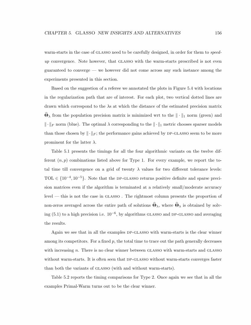
CHAPTER 5. GLASSO NEW INSIGHTS AND ALTERNATIVES 156
warm-starts in the case of glasso need to be carefully designed, in order for them to speed-
up convergence. Note however, that glasso with the warm-starts prescribed is not even
guaranteed to converge — we however did not come across any such instance among the
experiments presented in this section.
Based on the suggestion of a referee we annotated the plots in Figure 5.4 with locations
in the regularization path that are of interest. For each plot, two vertical dotted lines are
drawn which correspond to the λs at which the distance of the estimated precision matrix
Θλ from the population precision matrix is minimized wrt to the ‖ · ‖1 norm (green) and
‖ · ‖F norm (blue). The optimal λ corresponding to the ‖ · ‖1 metric chooses sparser models
than those chosen by ‖ ·‖F ; the performance gains achieved by dp-glasso seem to be more
prominent for the latter λ.
Table 5.1 presents the timings for all the four algorithmic variants on the twelve dif-
ferent (n, p) combinations listed above for Type 1. For every example, we report the to-
tal time till convergence on a grid of twenty λ values for two different tolerance levels:
TOL ∈ 10−4, 10−5. Note that the dp-glasso returns positive definite and sparse preci-
sion matrices even if the algorithm is terminated at a relatively small/moderate accuracy
level — this is not the case in glasso . The rightmost column presents the proportion of
non-zeros averaged across the entire path of solutions Θλ, where Θλ is obtained by solv-
ing (5.1) to a high precision i.e. 10−6, by algorithms glasso and dp-glasso and averaging
the results.
Again we see that in all the examples dp-glasso with warm-starts is the clear winner
among its competitors. For a fixed p, the total time to trace out the path generally decreases
with increasing n. There is no clear winner between glasso with warm-starts and glasso
without warm-starts. It is often seen that dp-glasso without warm-starts converges faster
than both the variants of glasso (with and without warm-starts).
Table 5.2 reports the timing comparisons for Type 2. Once again we see that in all the
examples Primal-Warm turns out to be the clear winner.

CHAPTER 5. GLASSO NEW INSIGHTS AND ALTERNATIVES 157
For n ≤ p = 1000, we observe that Primal-Warm is generally faster for Type-2 than
Type-1. This however, is reversed for smaller values of p ∈ 800, 500. Primal-Cold is has a
smaller overall computation time for Type-1 over Type-2. In some cases (for example n ≤
p = 1000), we see that Primal-Warm in Type-2 converges much faster than its competitors
on a relative scale than in Type-1 — this difference is due to the variations in the structure
of the covariance matrix.
p / nrelative Total time (secs) to compute a path of solutions Average %
error (TOL) Dual-Cold Dual-Warm Primal-Cold Primal-Warm Zeros in path
1000 / 50010−4 3550.71 6592.63 2558.83 2005.25
80.210−5 4706.22 8835.59 3234.97 2832.15
1000 / 100010−4 2788.30 3158.71 2206.95 1347.05
83.010−5 3597.21 4232.92 2710.34 1865.57
1000 / 150010−4 2447.19 4505.02 1813.61 932.34
85.610−5 2764.23 6426.49 2199.53 1382.64
800 / 50010−4 1216.30 2284.56 928.37 541.66
78.810−5 1776.72 3010.15 1173.76 798.93
800 / 80010−4 1135.73 1049.16 788.12 438.46
80.010−5 1481.36 1397.25 986.19 614.98
800 / 100010−4 1129.01 1146.63 786.02 453.06
80.210−5 1430.77 1618.41 992.13 642.90
500 / 20010−4 605.45 559.14 395.11 191.88
75.910−5 811.58 795.43 520.98 282.65
500 / 50010−4 427.85 241.90 252.83 123.35
75.210−5 551.11 315.86 319.89 182.81
500 / 80010−4 359.78 279.67 207.28 111.92
80.910−5 416.87 402.61 257.06 157.13
200 / 5010−4 65.87 50.99 37.40 23.32
75.610−5 92.04 75.06 45.88 35.81
200 / 20010−4 35.29 25.70 17.32 11.72
66.810−5 45.90 33.23 22.41 17.16
200 / 30010−4 32.29 23.60 16.30 10.77
66.010−5 38.37 33.95 20.12 15.12
Table 5.1: Table showing the performances of the four algorithms glasso (Dual-Warm/Cold)and dp-glasso (Primal-Warm/Cold) for the covariance model Type-1. We present the times (inseconds) required to compute a path of solutions to (5.1) (on a grid of twenty λ values) for different(n, p) combinations and relative errors (as in (5.40)). The rightmost column gives the averagedsparsity level across the grid of λ values. dp-glasso with warm-starts is consistently the winneracross all the examples.

CHAPTER 5. GLASSO NEW INSIGHTS AND ALTERNATIVES 158
0.4 0.6 0.8 1.0
100
200
300
400
500
600
700
0.4 0.6 0.8 1.0
020
040
060
080
010
00
0.2 0.4 0.6 0.8 1.0
5010
015
0
0.2 0.4 0.6 0.8 1.0
100
200
300
400
0.3 0.4 0.5 0.6 0.7 0.8 0.9 1.0
020
4060
8010
012
014
0
0.3 0.4 0.5 0.6 0.7 0.8 0.9 1.0
050
100
150
200
250
300
350
0.5 0.6 0.7 0.8 0.9 1.0
05
1015
Primal−ColdDual−ColdPrimal−WarmDual−Warm
0.4 0.5 0.6 0.7 0.8 0.9 1.0
05
1015
2025
Proportion of Zeros Proportion of Zeros
Tim
e in
Sec
onds
Tim
e in
Sec
onds
Tim
e in
Sec
onds
Tim
e in
Sec
onds
Type = 1 Type = 2
n = 500/p = 1000 n = 500/p = 1000
n = 500/p = 800 n = 500/p = 800
n = 200/p = 500 n = 200/p = 500
n = 50/p = 200 n = 50/p = 200
Figure 5.3: The timings in seconds for the four different algorithmic versions: glasso (with andwithout warm-starts) and dp-glasso (with and without warm-starts) for a grid of λ values on thelog-scale. [Left Panel] Covariance model for Type-1, [Right Panel] Covariance model for Type-2.The horizontal axis is indexed by the proportion of zeros in the solution. The vertical dashed linescorrespond to the optimal λ values for which the estimated errors ‖Θλ−Θ‖1 (green) and ‖Θλ−Θ‖F(blue) are minimum.

CHAPTER 5. GLASSO NEW INSIGHTS AND ALTERNATIVES 159
p / nrelative Total time (secs) to compute a path of solutions Average %
error (TOL) Dual-Cold Dual-Warm Primal-Cold Primal-Warm Zeros in path
1000 / 50010−4 6093.11 5483.03 3495.67 1661.93
75.610−5 7707.24 7923.80 4401.28 2358.08
1000 / 100010−4 4773.98 3582.28 2697.38 1015.84
76.7010−5 6054.21 4714.80 3444.79 1593.54
1000 / 150010−4 4786.28 5175.16 2693.39 1062.06
78.510−5 6171.01 6958.29 3432.33 1679.16
800 / 50010−4 2914.63 3466.49 1685.41 1293.18
74.310−5 3674.73 4572.97 2083.20 1893.22
800 / 80010−4 2021.55 1995.90 1131.35 618.06
74.410−5 2521.06 2639.62 1415.95 922.93
800 / 100010−4 3674.36 2551.06 1834.86 885.79
75.910−5 4599.59 3353.78 2260.58 1353.28
500 / 20010−4 1200.24 885.76 718.75 291.61
70.510−5 1574.62 1219.12 876.45 408.41
500 / 50010−4 575.53 386.20 323.30 130.59
72.210−5 730.54 535.58 421.91 193.08
500 / 80010−4 666.75 474.12 373.60 115.75
73.710−5 852.54 659.58 485.47 185.60
200 / 5010−4 110.18 98.23 48.98 26.97
73.010−5 142.77 133.67 55.27 33.95
200 / 20010−4 50.63 40.68 23.94 9.97
63.710−5 66.63 56.71 31.57 14.70
200 / 30010−4 47.63 36.18 21.24 8.19
65.010−5 60.98 50.52 27.41 12.22
Table 5.2: Table showing comparative timings of the four algorithmic variants of glasso and dp-glasso for the covariance model in Type-2. This table is similar to Table 5.1, displaying results forType-1. dp-glasso with warm-starts consistently outperforms all its competitors.
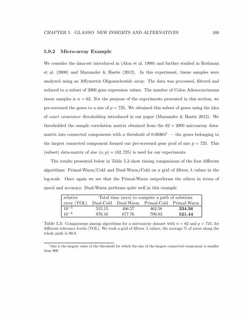
CHAPTER 5. GLASSO NEW INSIGHTS AND ALTERNATIVES 160
5.9.2 Micro-array Example
We consider the data-set introduced in (Alon et al. 1999) and further studied in Rothman
et al. (2008) and Mazumder & Hastie (2012). In this experiment, tissue samples were
analyzed using an Affymetrix Oligonucleotide array. The data was processed, filtered and
reduced to a subset of 2000 gene expression values. The number of Colon Adenocarcinoma
tissue samples is n = 62. For the purpose of the experiments presented in this section, we
pre-screened the genes to a size of p = 725. We obtained this subset of genes using the idea
of exact covariance thresholding introduced in our paper (Mazumder & Hastie 2012). We
thresholded the sample correlation matrix obtained from the 62 × 2000 microarray data-
matrix into connected components with a threshold of 0.003641 — the genes belonging to
the largest connected component formed our pre-screened gene pool of size p = 725. This
(subset) data-matrix of size (n, p) = (62, 725) is used for our experiments.
The results presented below in Table 5.3 show timing comparisons of the four different
algorithms: Primal-Warm/Cold and Dual-Warm/Cold on a grid of fifteen λ values in the
log-scale. Once again we see that the Primal-Warm outperforms the others in terms of
speed and accuracy. Dual-Warm performs quite well in this example.
relative Total time (secs) to compute a path of solutionserror (TOL) Dual-Cold Dual-Warm Primal-Cold Primal-Warm
10−3 515.15 406.57 462.58 334.5610−4 976.16 677.76 709.83 521.44
Table 5.3: Comparisons among algorithms for a microarray dataset with n = 62 and p = 725, fordifferent tolerance levels (TOL). We took a grid of fifteen λ values, the average % of zeros along thewhole path is 90.8.
1this is the largest value of the threshold for which the size of the largest connected component is smallerthan 800

CHAPTER 5. GLASSO NEW INSIGHTS AND ALTERNATIVES 161
5.10 Conclusions
This chapter explores some of the apparent mysteries in the behavior of the glasso al-
gorithm introduced in (Friedman, Hastie & Tibshirani 2007). These have been explained
by leveraging the fact that the glasso algorithm is solving the dual of the graphical lasso
problem (5.1), by block coordinate ascent. Each block update, itself the solution to a convex
program, is solved via its own dual, which is equivalent to a lasso problem. The optimization
variable is W, the covariance matrix, rather than the target precision matrix Θ. During the
course of the iterations, a working version of Θ is maintained, but it may not be positive
definite, and its inverse is not W. Tight convergence is therefore essential, for the solution
Θ to be a proper inverse covariance. There are issues using warm starts with glasso, when
computing a path of solutions. Unless the sequence of λs are sufficiently close, since the
“warm start”s are not dual feasible, the algorithm can get into trouble.
We have also developed two primal algorithms p-glasso and dp-glasso. The former
is more expensive, since it maintains the relationship W = Θ−1 at every step, an O(p3)
operation per sweep across all row/columns. dp-glasso is similar in flavor to glasso
except its optimization variable is Θ. It also solves the dual problem when computing its
block update, in this case a box-QP. This box-QP has attractive sparsity properties at both
ends of the regularization path, as evidenced in some of our experiments. It maintains a
positive definite Θ throughout its iterations, and can be started at any positive definite
matrix. Our experiments show in addition that dp-glasso is faster than glasso.
An R package implementing dp-glasso will be made available in CRAN.
5.A Appendix to Chapter 5
This section complements the examples provided in the chapter with further experiments
and illustrations.

CHAPTER 5. GLASSO NEW INSIGHTS AND ALTERNATIVES 162
5.A.1 Examples: Non-Convergence of glasso with warm-starts
This section illustrates with examples that warm-starts for the glasso need not converge.
This is a continuation of examples presented in Section 5.8.
Example 1:
We took (n, p) = (2, 5) and setting the seed of the random number generator in R as
set.seed(2008) we generated a data-matrix Xn×p with iid standard Gaussian entries. The
sample covariance matrix S is given below:
0.03597652 0.03792221 0.1058585 −0.08360659 0.1366725
0.03597652 0.03792221 0.1058585 −0.08360659 0.1366725
0.10585853 0.11158361 0.3114818 −0.24600689 0.4021497
−0.08360659 −0.08812823 −0.2460069 0.19429514 −0.3176160
0.13667246 0.14406402 0.4021497 −0.31761603 0.5192098
With q denoting the maximum off-diagonal entry of S (in absolute value), we solved (5.1)
using glasso at λ = 0.9×q. The covariance matrix for this λ was taken as a warm-start for
the glasso algorithm with λ′ = λ×0.01. The smallest eigen-value of the working covariance
matrix W produced by the glasso algorithm, upon updating the first row/column was:
−0.002896128, which is clearly undesirable for the convergence of the algorithm glasso .
This is why the algorithm glasso breaks down.
Example 2:
The example is similar to above, with (n, p) = (10, 50), the seed of random number generator
in R being set to set.seed(2008) and Xn×p is the data-matrix with iid Gaussian entries.
If the covariance matrix Wλ which solves problem (5.1) with λ = 0.9 × maxi 6=j |sij | is
taken as a warm-start to the glasso algorithm with λ′ = λ × 0.1 — the algorithm fails

CHAPTER 5. GLASSO NEW INSIGHTS AND ALTERNATIVES 163
to converge. Like the previous example, after the first row/column update, the working
covariance matrix has negative eigen-values.
5.B Further Experiments and Numerical Studies
This section is a continuation to Section 5.9, in that it provides further examples comparing
the performance of algorithms glasso and dp-glasso . The experimental data is generated
as follows. For a fixed value of p, we generate a matrix Ap×p with random Gaussian entries.
The matrix is symmetrized by A ← (A + A′)/2. Approximately half of the off-diagonal
entries of the matrix are set to zero, uniformly at random. All the eigen-values of the
matrix A are lifted so that the smallest eigen-value is zero. The noiseless version of the
precision matrix is given by Θ = A + τIp×p. We generated the sample covariance matrix
S by adding symmetric positive semi-definite random noise N to Θ−1; i.e. S = Θ−1 +N,
where this noise is generated in the same manner as A. We considered four different values
of p ∈ 300, 500, 800, 1000 and two different values of τ ∈ 1, 4.
For every p, τ combination we considered a path of twenty λ values on the geometric
scale. For every such case four experiments were performed: Primal-Cold, Primal-Warm,
Dual-Cold and Dual-Warm (as described in Section 5.9). Each combination was run 5 times,
and the results averaged, to avoid dependencies on machine loads. Figure 5.4 shows the
results. Overall, dp-glasso with warm starts performs the best, especially at the extremes
of the path. We gave some explanation for this in Section 5.6. For the largest problems
(p = 1000) their performances are comparable in the central part of the path (though
dp-glasso dominates), but at the extremes dp-glasso dominates by a large margin.

CHAPTER 5. GLASSO NEW INSIGHTS AND ALTERNATIVES 164
0.0 0.2 0.4 0.6 0.8 1.0
12
34
5p = 300
0.0 0.2 0.4 0.6 0.8 1.0
12
34
5
p = 300
0.0 0.2 0.4 0.6 0.8 1.0
510
1520
25
p = 500
0.0 0.2 0.4 0.6 0.8 1.0
510
1520
25
p = 500
0.0 0.2 0.4 0.6 0.8 1.0
2040
6080
100
p = 800
0.0 0.2 0.4 0.6 0.8 1.0
2040
6080
100
p = 800
0.0 0.2 0.4 0.6 0.8 1.0
5010
015
020
0
p = 1000
Primal−ColdDual−ColdPrimal−WarmDual−Warm
0.0 0.2 0.4 0.6 0.8 1.0
5010
015
020
0
p = 1000
Proportion of Zeros Proportion of Zeros
Tim
e in
Sec
onds
Tim
e in
Sec
onds
Tim
e in
Sec
onds
Tim
e in
Sec
onds
τ = 1 τ = 4
Figure 5.4: The timings in seconds for the four different algorithmic versions glasso (with andwithout warm-starts) and dp-glasso (with and without warm-starts) for a grid of twenty λ valueson the log-scale. The horizontal axis is indexed by the proportion of zeros in the solution.

Bibliography
Abernethy, J., Bach, F., Evgeniou, T. & Vert, J.-P. (2009), ‘A new approach to collabo-
rative filtering: operator estimation with spectral regularization’, Journal of Machine
Learning Research 10, 803–826.
Alon, U., Barkai, N., Notterman, D. A., Gish, K., Ybarra, S., Mack, D. & Levine, A. J.
(1999), ‘Broad patterns of gene expression revealed by clustering analysis of tumor
and normal colon tissues probed by oligonucleotide arrays’, Proceedings of the National
Academy of Sciences of the United States of America 96(12), 6745–6750.
URL: http://dx.doi.org/10.1073/pnas.96.12.6745
Argyriou, A., Evgeniou, T. & Pontil, M. (2007), Multi-task feature learning, in ‘Advances
in Neural Information Processing Systems 19’, MIT Press.
Argyriou, A., Evgeniou, T. & Pontil, M. (2008), ‘Convex multi-task feature learning’, Ma-
chine Learning 73(3), 243–272.
Bach, F. (2008), ‘Consistency of trace norm minimization’, Journal of Machine Learning
Research 9, 1019–1048.
Banerjee, O., Ghaoui, L. E. & d’Aspremont, A. (2008), ‘Model selection through sparse
maximum likelihood estimation for multivariate gaussian or binary data’, Journal of
Machine Learning Research 9, 485–516.
165

BIBLIOGRAPHY 166
Beck, A. & Teboulle, M. (2009), ‘A fast iterative shrinkage-thresholding algorithm for linear
inverse problems’, SIAM J. Imaging Sciences 2(1), 183–202.
Bell, R. M. & Koren., Y. (2007), Lessons from the Netflix prize challenge, Technical report,
AT&T Bell Laboratories.
Bollobas, B. (1998), Modern graph theory, Springer, New York.
Borwein, J. & Lewis, A. (2006), Convex Analysis and Nonlinear Optimization, Springer.
Boyd, S. & Vandenberghe, L. (2004), Convex Optimization, Cambridge University Press.
Breiman, L. (1996), ‘Heuristics of instability and stabilization in model selection’, Annals
of Statistics 24, 2350–2383.
Burer, S. & Monteiro, R. D. (2005), ‘Local minima and convergence in low-rank semidefinite
programming’, Mathematical Programming 103(3), 427–631.
Cai, J.-F., Candes, E. J. & Shen, Z. (2010), ‘A singular value thresholding algorithm for
matrix completion’, SIAM Journal on Optimization 20(4), 1956–1982.
URL: http://dx.doi.org/10.1137/080738970
Candes, E. J. & Tao, T. (2009), ‘The power of convex relaxation: near-optimal matrix
completion’, IEEE Transactions on Information Theory 56(5), 2053–2080.
Candes, E. J., Wakin, M. B. & Boyd, S. (2008), ‘Enhancing sparsity by reweighted l1
minimization’, Journal of Fourier Analysis and Applications 14(5), 877–905.
Candes, E. & Recht, B. (2008), ‘Exact matrix completion via convex optimization’, Foun-
dations of Computational Mathematics 9, 717–772.
Chen, S. & Donoho, D. (1994), On basis pursuit, Technical report, Department of Statistics
Stanford University.

BIBLIOGRAPHY 167
Cox, D. & Wermuth, N. (1996), Multivariate Dependencies, Chapman and Hall, London.
DeCoste, D. (2006), Collaborative prediction using ensembles of maximum margin matrix
factorizations, in ‘Proceedings of the 23rd International Conference on Machine Learn-
ing’, ACM, pp. 249–256.
Dempster, A., Laird, N. & Rubin, D. (1977), ‘Maximum likelihood from incomplete data
via the EM algorithm (with discussion)’, Journal of the Royal Statistical Society Series
B 39, 1–38.
Donoho, D. (2006), ‘For most large underdetermined systems of equations, the minimal
ℓ1-norm solution is the sparsest solution’, Communications on Pure and Applied Math-
ematics 59, 797–829.
Donoho, D., Johnstone, I., Kerkyachairan, G. & Picard, D. (1995), ‘Wavelet shrinkage;
asymptopia? (with discussion)’, Journal of the Royal Statistical Society: Series B
57, 201–337.
Efron, B., Hastie, T., Johnstone, I. & Tibshirani, R. (2004), ‘Least angle regression (with
discussion)’, Annals of Statistics 32(2), 407–499.
Fan, J. & Li, R. (2001), ‘Variable selection via nonconcave penalized likelihood and its oracle
properties’, Journal of the American Statistical Association 96(456), 1348–1360(13).
Fazel, M. (2002), Matrix Rank Minimization with Applications, PhD thesis, Stanford Uni-
versity.
Frank, I. & Friedman, J. (1993), ‘A statistical view of some chemometrics regression tools
(with discussion)’, Technometrics 35(2), 109–148.
Friedman, J. (2008), Fast sparse regression and classification, Technical report, Department
of Statistics, Stanford University.

BIBLIOGRAPHY 168
Friedman, J., Hastie, T., Hoefling, H. & Tibshirani, R. (2007), ‘Pathwise coordinate opti-
mization’, Annals of Applied Statistics 2(1), 302–332.
Friedman, J., Hastie, T. & Tibshirani, R. (2007), ‘Sparse inverse covariance estimation with
the graphical lasso’, Biostatistics 9, 432–441.
Friedman, J., Hastie, T. & Tibshirani, R. (2009), glmnet: Lasso and elastic-net regularized
generalized linear models. R package version 1.1-4.
URL: http://www-stat.stanford.edu/ hastie/Papers/glmnet.pdf
Gao, H.-Y. & Bruce, A. G. (1997), ‘Waveshrink with firm shrinkage’, Statistica Sinica
7, 855–874.
Gazit, H. (1991), ‘An optimal randomized parallel algorithm for finding connected compo-
nents in a graph’, SIAM J. on Computing 20(6), 1046–1067.
Grant, M. & Boyd., S. (2009), ‘CVX: Matlab software for disciplined convex programming’.
Web page and software available at http://stanford.edu/∼boyd/cvx.
Hastie, T., Tibshirani, R. & Friedman, J. (2009), The Elements of Statistical Learning,
Second Edition: Data Mining, Inference, and Prediction (Springer Series in Statis-
tics), 2 edn, Springer New York.
URL: ”http://www.amazon.ca/exec/obidos/redirect?tag=citeulike09-
20&path=ASIN/0387848576”
Huang, J., Ma, S. & Zhan, C.-H. (2008), ‘Adaptive lasso for sparse high-dimensional re-
gression models’, Statistica Sinica 18, 1603–1618.
Ji, S. & Ye, J. (2009), An accelerated gradient method for trace norm minimization, in
‘Proceedings of the 26th International Conference on Machine Learning’, pp. 457–464.
Keshavan, R. H., Oh, S. & Montanari, A. (2009), ‘Matrix completion from a few entries’,
IEEE Transactions on Information Theory 56(6), 2980–2998.

BIBLIOGRAPHY 169
Knight, K. & Fu, W. (2000), ‘Asymptotics for lasso-type estimators’, Annals of Statistics
28(5), 1356–1378.
Larsen, R. (2004), ‘Propack-software for large and sparse svd calculations’. Available at
http://sun.stanford.edu/∼rmunk/PROPACK.
Larsen, R. M. (1998), Lanczos bidiagonalization with partial reorthogonalization, Technical
Report DAIMI PB-357, Department of Computer Science, Aarhus University.
Lauritzen, S. (1996), Graphical Models, Oxford University Press.
Liu, J., Ji, S. & Ye, J. (2009), SLEP: Sparse Learning with Ef-
ficient Projections, Arizona State University. Available at
http://www.public.asu.edu/∼jye02/Software/SLEP.
Liu, Z. & Vandenberghe, L. (2009), ‘Interior-point method for nuclear norm approxima-
tion with application to system identfication’, SIAM Journal on Matrix Analysis and
Applications 31(3), 1235–1256.
Lu, Z. (2009), ‘Smooth optimization approach for sparse covariance selection’, SIAM J. on
Optimization 19, 1807–1827.
URL: http://portal.acm.org/citation.cfm?id=1654243.1654257
Lu, Z. (2010), ‘Adaptive first-order methods for general sparse inverse covariance selection’,
SIAM J. Matrix Anal. Appl. 31, 2000–2016.
URL: http://dx.doi.org/10.1137/080742531
Ma, S., Goldfarb, D. & Chen, L. (2011), ‘Fixed point and bregman iterative methods for
matrix rank minimization’, Mathematical Programmming 128(1-2), 321–353.
URL: http://dx.doi.org/10.1007/s10107-009-0306-5
Mazumder, R., Friedman, J. & Hastie, T. (2011), ‘Sparsenet: coordinate descent with
non-convex penalties’, Journal of the American Statistical Association (Theory and

BIBLIOGRAPHY 170
Methods) 106(495), 1125–1138.
URL: doi:10.1198/jasa.2011.tm09738
Mazumder, R. & Hastie, T. (2011), ‘The graphical lasso : New insights and alternatives’,
available at arXiv:1111.5479v2 .
URL: http://arxiv.org/abs/1111.5479v2
Mazumder, R. & Hastie, T. (2012), ‘Exact covariance thresholding into connected compo-
nents for large-scale graphical lasso’, Journal of Machine Learning Research 13, 781794.
URL: http://arxiv.org/abs/1108.3829
Mazumder, R., Hastie, T. & Tibshirani, R. (2010), ‘Spectral regularization algorithms for
learning large incomplete matrices’, Journal of Machine Learning Research 11, 2287–
2322.
URL: http://jmlr.csail.mit.edu/papers/volume11/mazumder10a/mazumder10a.pdf
Meinshausen, N. & Buhlmann, P. (2006), ‘High-dimensional graphs and variable selection
with the lasso’, Annals of Statistics 34, 1436–1462.
Nesterov, Y. (2003), ‘Introductory lectures on convex optimization: Basic course’, Kluwer,
Boston .
Nesterov, Y. (2005), ‘Smooth minimization of non-smooth functions’, Math. Program., Serie
A 103, 127–152.
Nesterov, Y. (2007), Gradient methods for minimizing composite objective function, Tech-
nical report, Center for Operations Research and Econometrics (CORE), Catholic
University of Louvain. Tech. Rep, 76.
Nikolova, M. (2000), ‘Local strong homogeneity of a regularized estimator’, SIAM J. Appl.
Math. 61, 633–658.

BIBLIOGRAPHY 171
Osborne, M., Presnell, B. & Turlach, B. (2000), ‘A new approach to variable selection in
least squares problems’, IMA Journal of Numerical Analysis 20, 389–404.
Recht, B., Fazel, M. & Parrilo, P. A. (2007), ‘Guaranteed minimum-rank solu-
tions of linear matrix equations via nuclear norm minimization’. Available at
http://www.citebase.org/abstract?id=oai:arXiv.org:0706.4138.
Rennie, J. & Srebro, N. (2005), Fast maximum margin matrix factorization for collaborative
prediction, in ‘Proceedings of the 22nd International Conference on Machine Learning’,
ACM, pp. 713–719.
Rothman, A., Bickel, P., Levina, E. & Zhu, J. (2008), ‘Sparse permutation invariant covari-
ance estimation’, Electronic Journal of Statistics 2, 494–515.
Salakhutdinov, R., Mnih, A. & Hinton, G. E. (2007), Restricted Boltzmann machines for
collaborative filtering, in ‘Proceedings of the 24th International Conference on Machine
Learning’, AAAI Press, pp. 791–798.
Scheinberg, K., Ma, S. & Goldfarb, D. (2010), ‘Sparse inverse covariance selection via
alternating linearization methods’, NIPS pp. 1–9.
URL: http://arxiv.org/abs/1011.0097
She, Y. (2009), ‘Thresholding-based iterative selection procedures for model selection and
shrinkage’, Electronic Journal of Statistics .
SIGKDD, A. & Netflix (2007), Soft modelling by latent variables: the nonlinear iterative
partial least squares (NIPALS) approach, in ‘Proceedings of KDD Cup and Workshop’.
Available at http://www.cs.uic.edu/∼liub/KDD-cup-2007/proceedings.html.
Srebro, N., Alon, N. & Jaakkola, T. (2005), Generalization error bounds for collabora-
tive prediction with low-rank matrices, in ‘Advances in Neural Information Processing
Systems 17’, MIT Press, pp. 5–27.

BIBLIOGRAPHY 172
Srebro, N. & Jaakkola, T. (2003), Weighted low-rank approximations, in ‘Proceedings of
the 20th International Conference on Machine Learning’, AAAI Press, pp. 720–727.
Srebro, N., Rennie, J. & Jaakkola, T. (2005), Maximum-margin matrix factorization, in
‘Advances in Neural Information Processing Systems 17’, MIT Press, pp. 1329–1336.
Stein, C. (1981), ‘Estimation of the mean of a multivariate normal distribution’, Annals of
Statistics 9, 1131–1151.
Takacs, G., Pilaszy, I., Nemeth, B. & Tikk, D. (2009), ‘Scalable collaborative filtering
approaches for large recommender systems’, Journal of Machine Learning Research
10, 623–656.
Tarjan, R. E. (1972), ‘Depth-first search and linear graph algorithms’, SIAM Journal on
Computing 1(2), 146160.
Tibshirani, R. (1996), ‘Regression shrinkage and selection via the lasso’, Journal of the
Royal Statistical Society, Series B 58, 267–288.
Tibshirani, R. (2011), ‘Regression shrinkage and selection via the lasso: a retrospective’,
Journal of the Royal Statistical Society: Series B (Statistical Methodology) 73(3), 273–
282.
URL: http://dx.doi.org/10.1111/j.1467-9868.2011.00771.x
Troyanskaya, O., Cantor, M., Sherlock, G., Brown, P., Hastie, T., Tibshirani, R., Botstein,
D. & Altman, R. B. (2001), ‘Missing value estimation methods for DNA microarrays’,
Bioinformatics 17(6), 520–525.
Tseng, P. (2001), ‘Convergence of a block coordinate descent method for nondifferentiable
minimization’, Journal of Optimization Theory and Applications 109, 475–494.
Tseng, P. & Yun, S. (2009), ‘A coordinate gradient descent method for nonsmooth separable
minimization’, Mathematical Programming B 117, 387–423.

BIBLIOGRAPHY 173
van de Vijver, M. J., He, Y. D., van’t Veer, L. J., Dai, H., Hart, A. A., Voskuil, D. W.,
Schreiber, G. J., Peterse, J. L., Roberts, C., Marton, M. J., Parrish, M., Atsma, D.,
Witteveen, A., Glas, A., Delahaye, L., van der Velde, T., Bartelink, H., Rodenhuis, S.,
Rutgers, E. T., Friend, S. H. & Bernards, R. (2002), ‘A gene-expression signature as a
predictor of survival in breast cancer’, N. Engl. J. Med. 347, 1999–2009.
Witten, D. & Friedman, J. (2011), ‘A fast screening rule for the graphical lasso.’, Journal
of Computational and Graphical Statistics: In Press. . Report dated 3-12-2011.
Witten, D., Friedman, J. & Simon, N. (2011), ‘New insights and faster computations for
the graphical lasso’, Journal of Computational and Graphical Statistics 20(4), 892–900.
(Reference draft dated 9/8/2011).
Yuan, M. & Lin, Y. (2007), ‘Model selection and estimation in the gaussian graphical
model’, Biometrika 94(1), 19–35.
Yuan, X. (2009), ‘Alternating direction methods for sparse covariance selection’, Methods
(August), 1–12.
URL: http://www.optimization-online.org/DB-FILE/2009/09/2390.pdf
Zhang, C. H. (2010), ‘Nearly unbiased variable selection under mnimax concave penalty’,
Annals of Statistics 38(2), 894–942.
Zhang, C.-H. & Huang, J. (2008), ‘The sparsity and bias of the lasso selection in high-
dimensional linear regression’, Annals of Statistics 36(4), 1567–1594.
Zhang, T. (2009), Multi-stage convex relaxation for non-convex optimization, Technical
report, Rutgers Tech Report.
Zhao, P. & Yu, B. (2006), ‘On model selection consistency of lasso’, Journal of Machine
Learning Research 7, 2541–2563.

BIBLIOGRAPHY 174
Zhou, S., Rutimann, P., Xu, M. & Buhlmann, P. (2011), ‘High-dimensional covariance
estimation based on gaussian graphical models’, Journal of Machine Learning Research
999888, 2975–3026.
URL: http://dl.acm.org/citation.cfm?id=2078183.2078201
Zou, H. (2006), ‘The adaptive lasso and its oracle properties’, Journal of the American
Statistical Association 101, 1418–1429.
Zou, H., Hastie, T. & Tibshirani, R. (2007), ‘On the degrees of freedom of the lasso’, Annals
of Statistics 35(5), 2173–2192.
Zou, H. & Li, R. (2008), ‘One-step sparse estimates in nonconcave penalized likelihood
models’, The Annals of Statistics 36(4), 1509–1533.