topic 3 - heriotjphillips/das/dataanalysistopic3.pdf · probability distributions ... 3.3 the...

1

Topic 3

Probability Distributions

Contents

3.1 Discrete Random Variables . . . . . . . . . . . . . . . . . . . . . . . . . . . . . 2

3.1.1 Random Variables and Expected Value . . . . . . . . . . . . . . . . . . 2

3.1.2 The Binomial Probability Distribution . . . . . . . . . . . . . . . . . . . . 4

3.1.3 The Geometric Probability Distribution . . . . . . . . . . . . . . . . . . . 9

3.1.4 The Hypergeometric Distribution . . . . . . . . . . . . . . . . . . . . . . 11

3.1.5 The Poisson Distribution . . . . . . . . . . . . . . . . . . . . . . . . . . . 14

3.2 Continuous Random Variables . . . . . . . . . . . . . . . . . . . . . . . . . . . 18

3.2.1 The Uniform Probability Distribution . . . . . . . . . . . . . . . . . . . . 22

3.2.2 The Gamma Distribution . . . . . . . . . . . . . . . . . . . . . . . . . . . 23

3.2.3 The Chi-Square Distribution . . . . . . . . . . . . . . . . . . . . . . . . . 25

3.2.4 The Exponential Probability Distribution . . . . . . . . . . . . . . . . . . 25

3.2.5 The Weibull Distribution . . . . . . . . . . . . . . . . . . . . . . . . . . . 26

3.3 The Normal Distribution . . . . . . . . . . . . . . . . . . . . . . . . . . . . . . . 28

3.3.1 Everyday examples of Normal Distribution . . . . . . . . . . . . . . . . . 28

3.3.2 Drawing the Curve . . . . . . . . . . . . . . . . . . . . . . . . . . . . . . 30

3.3.3 Calculations Using Normal Distribution . . . . . . . . . . . . . . . . . . . 31

3.3.4 Properties of Normal Distribution Curves . . . . . . . . . . . . . . . . . 32

3.3.5 Link with Probability . . . . . . . . . . . . . . . . . . . . . . . . . . . . . 33

3.3.6 Upper and Lower Bounds . . . . . . . . . . . . . . . . . . . . . . . . . . 38

3.4 Summary . . . . . . . . . . . . . . . . . . . . . . . . . . . . . . . . . . . . . . . 41

2 TOPIC 3. PROBABILITY DISTRIBUTIONS

3.1 Discrete Random Variables

Many problems in statistics can be solved by classifying them into particular types. Forexample, in quality control the probability of finding faulty goods is an important issue.This is a standard situation where we are dealing with success or failure and there aretried and trusted approaches to tackling a problem like this (in fact it can be dealt with byusing the binomial distribution to be explained shortly). Since the number of successesor failures must necessarily be a whole number, the only probabilities we can calculateare things like "the probability of 5 failures". It does not make sense to deal with, forexample, 2.56 failures. Therefore, the numbers in question are not continuous and aredefined instead as discrete. A discrete set could be something like {0,1,2,3,4}.

We will consider many different probability distributions, some relevant to discreterandom variables and, in the next section, others using the continuous type.

3.1.1 Random Variables and Expected Value

A random variable is a function taking numerical values which is defined over a samplespace. Simple random variables could be the temperature of a chemical process or thenumber of heads when a coin is tossed twice (0,1 or 2). Such a random variable iscalled discrete if it only takes countably many values.

Example

Problem:

A quality control engineer checks randomly the content of bags, each of whichcontains 100 resistors. He selects 10 resistors and measures whether they match thespecification (exact value plus or minus 10% tolerance).

Solution:

The number of resistors not matching the specification is a discrete random variable. (Itcan be anything from 0 to 10). Another random variable would be the function takingvalues 0 and 1, for the outcomes that there are faulty resistors in the bag, or not.

The probability distribution of a random variable is a table, graph, or formula that givesthe probability �� for each possible value of the random variable � . The requirementsare that� 0 � �� 1, i.e., the probability must lie between 0 and 1, and that�� .For a discrete random variable � with probability distribution �� the expected value (ormean) is defined as ��

all x

� ��!��c"

HERIOT-WATT UNIVERSITY 2004

3.1. DISCRETE RANDOM VARIABLES 3

The variance of a discrete random variable # with probability distribution $�%�#�& is definedas '�(*) +-, %�#/.102& (43the standard deviation is defined as 5 +6, %�# .702& (43 .Example

Problem:

Consider the random variable which shows the outcome of rolling a die and calculatethe Expected Value.

Solution:

Each possible outcome between 1 and 6 is equally likely, so $�%�#�& = 1/6 for # )�8:9<;=;=;=9�> .For the expected value we calculate+ %�#& )@?ACBDB<E # ; $�%�#&)!8:; 8>/F@G ; 8> F ;=;=; F >H; 8>) G 8>)JIH;DKClearly this is a statistic like "the average number of children in a family in the UK is 2.4"which is a single result that cannot happen, but it does give a mean value.

Let # be any discrete random variable with probability distribution $�%�#�& , and let L be anyfunction of # . Theexpected value of LM%�#& is defined as+ N LO%�#�&QP )R?

all x

LJ%�#&�S�$!%�#&Example:

Suppose we are rolling a die for gambling. If we roll 1,2, or 3 we lose 1 pound, ifwe roll 4 or 5 we win 1 pound, and if we roll 6 we will win 2 pounds. The functionLM%�#�& , sending each possible outcome 1,.....,6 to the win -1,-1,-1,1,1,2 is a function of therandom variable # , and the expected value+ %TLO%�#�&U& ) ?

all x

g % x &�S�$�%�#&) . 8 S 8> F %V. 8 &�S 8>/F 8 S 8>WF 8 S 8>/F@G S 8>) 8>is the average value that we are going to win (or lose) in each round of the game. (Inother words, 17p here)

cX



The following is a list of basic properties of expected values:Y@Z/[�\^]`_ \ , for every constant \ ;Y@Z/[�\4a]`_b\4Zc[�a] , for every constant \ ;Y@Z/d eHfg[�a]ihjelkm[�a]Qn�_ Z/d eHfg[�a]Qnoh@Z/d elkp[�a]Qn ,for any two functions eqf<r�e:k on a .

It follows the important formula used in many calculations thats k _ ZutDa k4vxw1yikFor the proof of this formula note thats k _zZ6{|[�a w1y ] k4} _ Z t a k wj~�y a!h y k4v_zZ t a k4v wj~�y Z�d a�noh y k Z�d��4n_zZ t a k4v wj~�y�y h y kActivity

An insurance company plans to introduce a new life insurance scheme for people aged50. The scheme will require a customer to pay a single premium when they reach theage of 50. If the customer dies within the next 10 years their heirs will receive � 10 000.If they don’t die they receive nothing.

From actuarial life tables the company knows that 15% of people aged 50 will die beforethey are 60.

Ignoring administrative costs, etc., what minimum premium should the company chargethe customer?

3.1.2 The Binomial Probability Distribution

The following statistical experiments have all common features:Y Tossing a coin 10 times.Y Asking 100 people on Princes Street in Edinburgh if they know that Madonna’swedding took place in a Scottish castle.Y Checking whether or not batches of transistors contain faulty transistors.

These experiments or observations are all examples of what is called abinomial experiment(the corresponding discrete random variable is called abinomial random variable). The examples have the following common characteristics:Y The experiment consists of � identical trials.Y In each trial there are exactly two possible outcomes (yes/no, pass/failure, or

success/failure).

c�


3.1. DISCRETE RANDOM VARIABLES 5� The probability of success is usually referred to as � and the probability of failureas � , with �� .� The discrete (binomial) random variable � is the number of successes in the �trials.

The binomial probability distributionis given by the formula ��J�� R� ��l��p��H�� <�=�=�=�� where� � is the probability of a success in a single trial, and �J� ��¡� ;� � is the number of trials; and� � is the number of successes; and� � � �R� is the binomial coefficient given by the number �p¢�:¢ (n - x)!

The expected value (mean) and standard deviation are given by the formulae £¤�¥�o�and ¦§�©¨ �o�ª�Example

Problem:

Tests show that about 20% of all private wells in some specific region are contaminated.What are the probabilities that in a random sample of 4 wells:

a) exactly 2

b) fewer than 2

c) at least 2

wells are contaminated?

Solution:

The random variable "number of contaminated wells" is clearly modelled by a binomialrandom variable. The probability that one particular well is contaminated is independentof the probability that some other well is contaminated, and for each well this probabilityis 0.2. Thus the parameters for the distribution are ��« and �¬� � �D .

a) ® ��¡�Rm�`�°¯ «:± � �D:² � �D³�´ � ²� «qµHµDHµ � �D ² � �D³ ²� «W¶§·!¶1� � �D ² � �D³ ²�J¸H� � �D ² � � �D³ ²� � �¹�^ºl·l¸c»



b) ¼ ½�¾§¿�ÀmÁ�ÂO¼ ½�¾�Â ÃpÁiÄ�¼ ½�¾�Â�ÅÆÁÂ°ÇÉÈÃmÊ ÃoËDÀ:Ì^ÃoËDÍ�ÎxÄÏÇzÈ Å^Ê ÃoËDÀÑÐCÃoËDÍ:ÒÂOÃoËDÍoÅ^ÓlÀc) ¼ ½�¾ÁÕÔ�ÀmÁ`Âz¼ ½�¾�ÂbÀmÁiÄÖ¼ ½�¾¡Âb×mÁiÄÖ¼/½�¾¡Â È ÁÂzÃoË¹Å^Øl×lÙzÄ ÇÉÈ×lÊ ÃoËDÀ Ò ÃoËDÍ Ð Ä ÇÉÈÃpÊ ÃoËDÀ Î ÃoËDÍ ÌÂzÃoË¹Å^Í:ÃmÍ

Expected value (mean) of binomial Ú Â ÛoÜ so this gives a value of 4 Ý 0.2 = 0.8

The following figure shows the graph for the corresponding probability distribution. (i.e.it shows the probabilities for x = 0, 1, 2, 3 and 4.)

00

0.1

0.4

0.2

0.3

41 2 3

outcome

prob

abili

ty

The graph can be shown in several different ways, e,g. using lines or points rather thanthe "bars".

cÞ



00

0.4

0.2

41 2 3

outcome

prob

abili

ty

00

0.1

0.25

0.4

0.05

0.2

0.3

0.45

4

0.15

0.35

0.5 1 1.5 2 2.5 3 3.5

The following graphs show binomial distributions for different values n and p, where p isalways on the y-axis and the random variable on the x-axis.

cß



00

0.2

0.1

outcome

prob

abili

ty

2 4 6 8 10 00

0.2

0.1

outcome

prob

abili

ty2 4 6 8 10

n = 10, p = 0.7 n = 10, p = 0.7

0 2 4 6 8 100

0.1

0.2

0.05

0.15

0.25

0 2 4 6 8 100

0.1

0.2

0.05

0.15

0.25

n = 10, p = 0.5 n = 10, p = 0.5

0 5 10 15 20 250

0.1

30 0 5 10 15 20 250

0.1

30

n = 30, p = 0.7 n = 30, p = 0.7

cà



Activity

Q1: In a large school it was reported that 1 out of 3 pupils take school meals regularly.In a random sample of 20 pupils from this school, calculate the probability that exactly 5do not take school meals regularly.á�â�ãä�å æ�çã ç â æ¡è ã�ä çêépë â�ì è é ä|íÑî ë å ï:ðoçñ ç ì ñ ç ðoòDólómô�õgðoòDölölöÑ÷Qõ å ðoòøðlðlð ìúù ð ñQ2:

A company provides an emergency service to domestic customers to repair applianceslike fridges, freezers etc. on site. The company offers a guaranteed same-day response.One day the company gets 20 requests for a call-out.

There are currently 25 authorised repair technicians on their payroll. From records, ithas been estimated that the probability of a technician not being available for work is 0.1.What is the probability that there will be enough technicians to meet demand? (Eachtechnician does only one job a day).

3.1.3 The Geometric Probability Distribution

Again we start with a typical application:

Example:

Customers wait in line to be served by a bank teller. Per minute the probability thata customer is served is 10%. What is the probability that a customer has to wait 15minutes before being served?

Such and similar events are modeled by the geometric probability distribution.Eachtime interval we have an ‘independent experiment’ which can succeed or fail withsuccess probability á (as for the binomial probability distribution). To be successful inthe ã th try we need ã è ì failures (with probability û åüá è ì ) and one success (withprobability á ).The data for the geometric probability distribution areý P(x) = pqx-1, for x = 1, 2, .....,

where ã is the number of trials until the first success; andýÖþ = 1/ÿ , andý��å � �ÿ�� .

c�



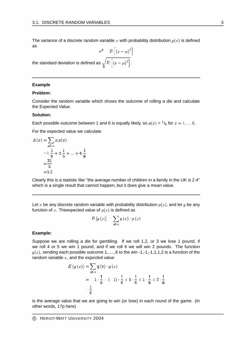
Figure 3.1: Geometric probability distribution, �� Example

Problem:

The average life expectancy of a fuse is 15 months. What is the probability that the fusewill last exactly 20 months?

Solution:

We have that � = 15 (months), or � = 1/15, which is the probability that a fuse will break.

For � = 20 we obtain �� "!$#&%('")which is approximately 0.018.

For * we find + � �,.-/�102�3054 . The two graphs Figure 3.2 Figure 3.3 below show theprobability distribution and the cumulative distribution, which is the function showing foreach possible value � of the random variable the function

�6� � ’ 78�"� .

c9



Figure 3.2: Geometric probability distribution, :;=<?> <A@

Figure 3.3: Geometric cumulative distribution, :B; < > <[email protected] The Hypergeometric Distribution

The binomial and the geometric probability distribution are to be applied if, afterobserving a result, the sample is put back into the population. However, in practice,we often sample without replacement:C If we test a bag of 1000 resistors whether they meet certain specifications we

usually will not put back the tested items.

cD


12 TOPIC 3. PROBABILITY DISTRIBUTIONSE Suppose people are randomly selected on Princes Street in Edinburgh to fill in aquestionnaire about a new product. When people are approached they are usuallyfirst asked whether they have already taken part in this marketing research.E A big manufacturing company maintains their machines on a regular basis.Suppose that on average 15% of the machines need repair. What is the probabilitythat among the five machines inspected this week, one of them needs repair?E A box of 1000 fuses is tested one by one until the first defective fuse is found.Supposing that about 5% of the fuses are defective, what is the probability that adefective fuse is among the first 5 fuses tested?

Such and similar random variables have a hypergeometric probability distribution.

The hypergeometric probability distribution is a discrete distribution that modelssampling without replacement.E The populations consists if F objects.E The possible outcomes of the experiment are success or failure.E Each sample of size G is equally likely to be drawn.

The formula for the hypergeometric probability distribution is

HJILKNMPORQ�SK�T Q FVU SGBU KWTQ F G T XZY X GBU[F]\ S_^ K ^ G X SwhereE F is the number of elements in the population;E S is the number in the population for success;E G is the number of elements drawn; andE`K is the number of successes in the G randomly drawn elements.

The mean and standard deviation are given byabO G SF XZc Ged�f O S I FgU S M G I FVU�G MFih I FVU8j MIf we write HOlknm�o then expected value and standard deviation becomea = G H and f Oqp FgUrGFsU�j G H_I j U HNMThis shows that the binomial and the hypergeometric distributions have the same

expected value, but different standard deviations. The correction factor t onuwvonu"x is

cy



less than z , but close to z if { is small relative to | . The following two graphsFigure 3.4 Figure 3.5 show the binomial and the hypergeometric distribution for differentparameters:

Figure 3.4: Comparing the binomial and the hypergeometric distribution,{b}~z,� ��|�}�� &��}~z,� ��Z}��

Figure 3.5: Comparing the binomial and the hypergeometric distribution,{b}~z,� ��|�}~z,�� &�J}�� }�� c�



Examples

1.

Problem:

A retailer sells computers. He buys lots of 10 motherboards from a manufacturer whosells them cheaply, but offers low quality only. Suppose the current lot contains onedefective item. If the retailer usually tests 4 items per lot, what is the probability that thelot is accepted?

Solution:

Here ��~�,� , ��~� , and �b�.� , and we are looking for �=�L��5� , which is

��L�B�� ¡ �,��¢ � �n£ � £¥¤¦£¨§©£¥ª� £�«l£�¬l£,� � £�«l£�¬ £,��,�£ � £¥¤¦£¨§� ª�,�We would use the same calculation if we would only know thaton average 10% of themotherboards are faulty.

2.

Problem:

We test lots of 100 fuses. On average 5% of the fuses are defective. If we test 4 fuses,what is the probability that we accept the current lot?

Solution:

Again, the random variable is hypergeometric, and since � � �,�� is large we canassume that there are 5 defective fuses in this lot. We find

��L�� l®� � ¡ � ®® ¢¡ �,��® ¢ � ¯(°± ° ¯(°³² ¯(°¯(° ² ± °´A±&± °¯(° ² ¯(°� � ®¶µ � � µ � ¬ µ � « µ � ��,�� µ �� µ � ¤ µ � § µ � ª· � ¸¹§�ª � ªLater we will see how reliable this value is, as we don’t know the exact number of faultyfuses in this lot.

3.1.5 The Poisson Distribution

The Poisson probability distribution provides a model for the frequency of events,like the number of people arriving at a counter, the number of plane crashes per month,or the number of micro-cracks in steel. (Micro-cracks in steel wheels of a Germanhigh-speed train ICE led to a disastrous rail accident in 1998 killing 101 people.) Thecharacteristics of a Poisson random variable are as follows:

cº


3.1. DISCRETE RANDOM VARIABLES 15» The experiment consists of counting events in a particular unit (time, area, volume,etc.).» The probability that an event occurs in a given unit is the same for every unit.» The number of events that occur in one unit is independent of the number of eventsthat occur in other units

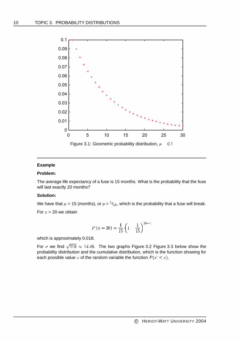
The Poisson probability distribution with parameter ¼ is given by the formula½J¾L¿NÀPÁ ¼wÂ�Ã�ÄÆÅ¿ÈÇÊÉ ¾L¿BÁ�Ë É�Ì�ÉÎÍÐÏÑÏÑÏÑÏ Àwhere Ã is the mathematical constant 2.71828..... The expected value and standarddeviation are Ò = ¼ and Ó Á~Ô ¼Example

Problem:

Suppose customers arrive at a counter at an average rate of 6 per minute, and supposethat the random variable ’customer arrival’ has a Poisson distribution. What is theprobability that in a half-minute interval at most one new customer arrives?

Solution:

Here ¼ = 6/2 = 3 customers per half-minute. SoÕ ¾L¿bÖ Ì À�Á Õ ¾×¿Á�Ë5ÀeØ Õ ¾L¿Á Ì ÀÁ Ã�ÄÆÙ�Ú�ÛË Ç Ø Ã�ÄÆÙ,Ú�ÜÌ ÇÁÞÝÃ Ùwhich equals approximately 0.1991.

The following graphs show the probability distribution ½ß¾L¿NÀ for this example, and thecumulative distributionà ¾L¿"ÀPÁ�á Â,âäãwÂ ½J¾L¿Æå�ÀNote that the highest outcome on the graph is 15 and that its probability is almostnegligible. In theory there is no upper limit on the graphs, but they have to stopsomewhere!

cæ



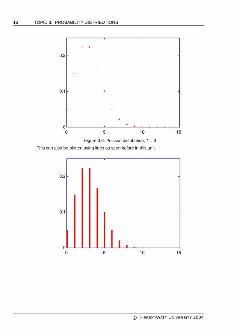
Figure 3.6: Poisson distribution, ç = 3

This can also be plotted using lines as seen before in this unit.

0 150

5 10

0.2

0.1

cè



The cumulative distribution can be shown as:

4

Figure 3.7: Cumulative Poisson distribution, é = 3

or alternatively, it can be drawn as:

0 150

0.4

1

5 10

0.2

0.6

0.8

Now, as a theoretical example we will verify that the Poisson probability distribution p(x)really is a distribution, and that the mean is é . The reader not familiar with infinite sumsshould skip the rest of this subsection.

cê



We note first that 0 ë p(x) for all values of x. Also, since we have the infinite sumì�í�î ïðñ�òNó³ô ñõÈöwe can calculate ÷ î�ì�øÆí5ì�í�î�ì�øÆí�ïðñ�òNó ô ñõùö îúïðñ�òNó ì øÆí ô ñõÈö îúïðñ�òNó¨ûJü õNýwhich shows that p(x) ë 1 andþ�ÿ��

x ûJü õNý�î÷.

For the mean we calculate � ü õNýPî ïðñ�òNó õ ì øÆí ô ñõùöî�� ïðñ�òNó õ ì øÆí ô ñõÈöî ïðñ�òNó õ ì øÆí ô ñ ø�ü õ� ÷ ý öî ô ïðñ�òNó õ ì øÆí ô ñõÈöî ôHere from line 2 to line 3 we cancelled x and took out one ? in the numerator, and in thenext step replaced x-1 (running through x = 1,2,...) by x (running through x = 0,1,....).

Activity

Emails come in to a university at a rate of 3 per minute. Assuming a Poisson distribution,calculate the probability that in any two-minute period, more than 2 emails arrive.

3.2 Continuous Random Variables

Many random variables arising in practice are not discrete. Examples are the strengthof a beam, the height of a person, the capacity of a conductor, or time it takes to accessmemory, etc. Such random variables are called continuous.

A practical problem arises, as it is impossible to assign finite amounts of probabilities touncountably many values of the real axis (or some interval) so that the values add up to1. Thus, continuous probability distributions are usually based on cumulative distributionfunctions.

c�


3.2. CONTINUOUS RANDOM VARIABLES 19

The cumulative distribution �� of a random variable � is the function �� .The following graphs Figure 3.8 Figure 3.9 show the binomial probability distributionwith �� , !"�#�%$�& , and the corresponding cumulative distribution, and as a secondexample, a Poisson distribution and the corresponding cumulative distribution. Bothdistributions are, or course, discrete examples.

0 2 4 6 8 100

0.1

0.2

0.3

0.05

0.15

0.25

0.35

Figure 3.8: Binomial distribution, n = 10, p = 0.3

0 2 4 6 8 100

0.8

1

0.2

0.6

0.4

Figure 3.9: Cumulative binomial distribution, �'�(� �%)*!+��%$�&If is the cumulative distribution of a continuous random variable � then the density

c,



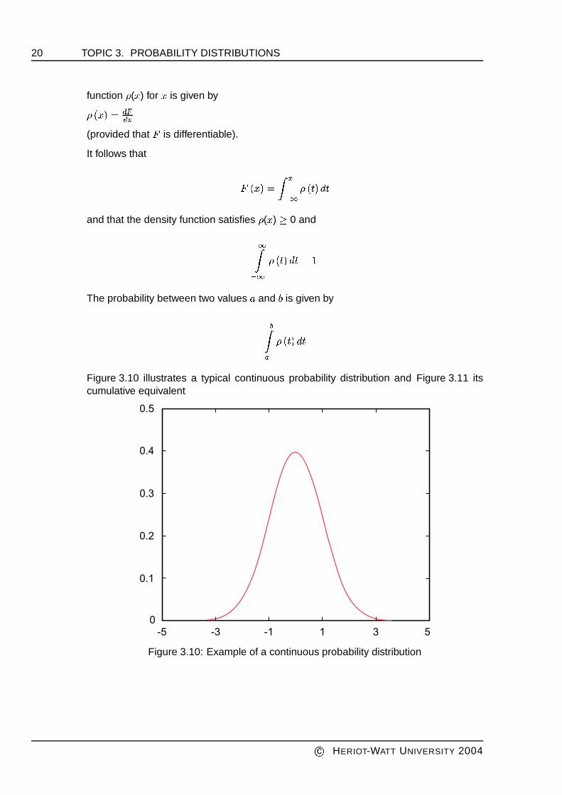
function - ( . ) for . is given by-0/1.�24365875:9(provided that ; is differentiable).

It follows that ;</*.243 = 9>@? -A/�B:2DCEBand that the density function satisfies - ( . ) F 0 and?=>@? -0/�B82%CEB43(GThe probability between two values H and I is given byJ= K -A/�B:2%CEBFigure 3.10 illustrates a typical continuous probability distribution and Figure 3.11 itscumulative equivalent

Figure 3.10: Example of a continuous probability distribution

cL



Figure 3.11: The corresponding cumulative distribution

Let us recall from calculus that an integral is a limit process of a summation. FindingM�N�O@PRQ4SUTWVYXZ@[W\ N�O�Q%]EOfor a continuous random variable is analogous to finding

FNx0

Q^S`_VbacV X \ N*OQfor a discrete random variable. Thus, we define theexpected value analogous to thediscrete case.

The expected value of a continuous random variableO

with density function \ (O) is given

by d S�efN�OQgS T [Z@[Wh \ N h Qi] hIf j is any function we define the expected value of j N�O�Q ase�k j N�OQml�SUT [Z@[ j N h Q \ N h Qi] hprovided that these integrals exist. The standard deviation is defined asn = o E p N x - d Qiqsr .ct



Note thatu"v�w*xYygz�x , for every constant x ;u"v�w*xs{�ygz|xsv}w�{�y , for every constant x ;u"v�~ �D��w*{�y��gw�{�yi��z�vf~ �D��w�{�yi�D��v�~ ��gw�{�ym� ,for any two functions �� b� on { .u"� 2 = v}~ { 2 � - � 2.

3.2.1 The Uniform Probability Distribution

If we select randomly a number in the interval [ � �� ] then the corresponding randomvariable { is called auniform random variable.Its density function is

�Aw�{�ygz �� ^� � if a � x � b

0 else

For the mean and standard deviation it can be shown that

� z � �"�� and � =b - a

2 � 3z � �� w�� y

Example

Problem:

A manufacturer of wires believes that one of her machines makes wires with diameteruniformly distributed between 0.98 and 1.03 millimeters.

Solution:

The mean of the thickness (in mm) is�:� �: 8¡��s� ¢:£� z �b¤¦¥�¥¨§and the standard deviation (in mm) is�'z#© ª w �b¤¦¥ � � ¥%¤�«�¬ y4 ¥%¤¦¥��¯®The density function for this uniform random variable is�0w1{�y4z �� :° z � ¥for 0.98 ± { ± 1.03, and ¥ elsewhere.

c²



And, for example, ³<´ µ'¶¸·b¹¦º�º¼»g½¿¾�ÀsÁ Â:ÃÄ@Å Æ´*Ç »DÈ ÇÉ ¾�Ê:Á À:ÀÀsÁ Â:Ã Æ

´*Ç »DÈ Ç½ ¾ Ê:Á À:ÀÀsÁ Â:ÃUË º�ÈÇ

½ Ë ºÍÌÎ·b¹¦º�ºÐÏÑº%¹�Ò�ÓÕÔ½0º%¹�ÖThe corresponding distribution is shown in uniformdistributionFigure 3.12

019

21

1.060.96 0.98 1 1.02

19.2

19.4

19.6

19.8

20

20.2

20.4

20.6

20.8

1.04

Figure 3.12: Uniform distribution, [0.98,1.03]

3.2.2 The Gamma Distribution

Many continuous random variables can only take positive values, like height, thickness,life expectations of transistors, etc. Such random variables are often modeled by gammatype random variables. The corresponding density functions contain two parameters× , Ø . The first is known as the shape parameter, the second as the scale parameter.

Figure 3.13 shows Gamma density function with ×Ù½Ú·bÛ�ÜDÛ�Ý and Ø ½(·

cÞ



Figure 3.13: Gamma density functions, ßÙàÚábâ�ãDâ�äbåEæèçêéëàÚáThe density function is given by

ì0í�îï à ðñò ñóî@ôDõö�÷ õùøúéûß�ü í ß ï if 0 ý x ý�þ , ß , é�ÿ 0

0 else

whereü í ß ï à�� ôDõö ÷ õ�� ç �is the gamma function, giving the gamma distribution its name.

The mean and standard deviation are à�ß�é and = � ß�é 2

The gamma function plays an important role in mathematics. It holds thatü í ß ��á ï à�ß�ü í ß ïandü í á ï à(áso that for integer values of ü í ß ï à í ß��<á ï�� . However, in general there is no closedform for the gamma function, and its values are approximated and taken from tables.

c�



Example

Problem:

A manufacturer of CPUs knows that the relative frequency of complaints from customers(in weeks) about total failures is modeled by a gamma distribution with � =2 and�

=4. Exactly 12 weeks after the quality control department was restructured the next(first) major complaint arrives. Does this suggest that the restructuring resulted in animprovement of quality control?

Solution:

We calculate � = � � =8 and �� ! #"%$& (' . The value ) =12 lies well within onestandard deviation from the (old) mean, so we would not consider it an exceptionalvalue. Thus there is insufficient evidence to indicate an improvement in quality controlgiven just this data.

3.2.3 The Chi-Square Distribution

The * 2 (chi-square) probability distribution plays an important role in statistics. Thedistribution is a special case of the gamma distribution for�+�-,. and

�=2

( / is called the number of degrees of freedom).

The density function is 021 * .43 �65 1 * .73 , 8#9;:=< 9?>(@.where5 1 * . 3 � :. , .�A�B , .DCFor mean and standard deviation one finds�E��/ and � = � 2 /3.2.4 The Exponential Probability Distribution

The exponential density function is a gamma density function with � =1,0 B ) C � < 9GFH� I x J 0

with mean � =�

and standard deviation � =�

.

The corresponding random variable models for example the length of time betweenevents (arrivals at a counter, requests to a CPU, etc) when the probability of an arrival inan interval is independent from arrivals in other intervals. This distribution also models

cK



the life expectancy of equipment or products, provided that the probability that theequipment will last L more time intervals is the same as for a new product (this holdsfor well-maintained equipment).

If the arrival of events follows a Poisson distribution with mean MN (arrivals per unitinterval), then the time interval between two successive arrivals is modeled by theexponential distribution with mean O .

3.2.5 The Weibull Distribution

The Weibull distribution is used extensively in reliability and life data analysis such assituations involving failure times of items. Since this failure time may be any positivenumber, the distribution is continuous. It has been used successfully to model suchthings as vacuum tube failures and ball bearing failures.

The formula for the probability density function initially looks quite complicated becauseit depends on three parameters, P , Q and R . It can, however, be made easier to workwith by assigning appropriate values to these.

The probability density function is:SUTWVYX[Z PR \ V^] QR _a`&b M�c b T4d�e&fg Xihwhere x jkQ and P and Rml 0

The value P is called the shape parameter, Q is the location parameter and R is the scaleparameter. The case where Q =0 and R =1 is called the standard Weibull distribution.Since the general form of probability functions can be expressed in terms of the standarddistribution, this simpler version is often used and the probability density function thenbecomes: SUTnV;X[Z P V `&b M c b;oqp hsrut VEvkwDx PEl wThe cumulative distribution function is:y TnVYX[Z{za] c b;o|p hsrThe mean of the distribution is given by:} \ P�~ zP _Where as usual, } Tn��X?Z�� L�� b M c b�� LFinally, the standard deviation is given by:

c�


3.2. CONTINUOUS RANDOM VARIABLES 27�� i��[�� k� ��6�� Some example graphs of the probability density function for various standard Weibulldistributions are shown below.

50

30

10

00 1 2 3 4 5

0.8

0.4

00 1 2 3 4 5

0.8

0.4

00 1 2 3 4 5

1

00 1 2 3 4 5

prob

abili

ty

prob

abili

ty

prob

abili

ty

prob

abili

ty

x x

x x

shape parameter 0.5 shape parameter 1

shape parameter 2 shape parameter 5

Example

Problem:

The time to failure (in hours) of bearings in a mechanical shaft is satisfactorily modelledas a Weibull random variable with � =0.5, =0 and ¡ =5000. Determine the probabilitythat a bearing lasts fewer than 6000 hours and also the mean time to failure.

Solution:

It can be shown that the cumulative distribution function is given by¢¤£W¥;¦?§ � ��¨&© £sª« ¦i¬This translates as: ¢£¯®±°&°&°#¦?§ � �m¨ © £4²¯³¯³¯³´ ³¯³¯³ ¦ ³¶µ ´The number calculates as 0.666.

c·



The mean time to failure is given by: ¸º¹�»[¼�½¿¾¼ ÀThis calculates as 5000?(3)=5000x2!=10000 hours.

Activity

Fans to cool microelectronics may fail in several ways and failure may be defineddifferently depending upon the applications. Fan failures typically include excessivevibration, noise, rubbing or hitting of the propeller, reduction in rotational speed, lockedrotor, failure to start, etc.

The time to failure (in hours) of a fan is satisfactorily modelled as a Weibull randomvariable with

¼=4.9, Á =0 and

¸=9780. Calculate the probability that a fan lasts longer

than 10000 hours and also the mean time to failure.

3.3 The Normal Distribution

3.3.1 Everyday examples of Normal Distribution

A number of continuous distributions have been defined in the previous section. By farthe most common to be used, however, is the Normal distribution and so it is describedin detail here

In day to day life much use is made of statistics, in many cases without the persondoing so even realising it. If you were to go into a shop and you noticed that everybodywaiting to be served was over 6 and a half feet tall, you would more than likely be a bitsurprised. You probably would have expected most people to be around the "average"height, maybe spotting just one or two people in the shop that would be taller than 6 anda half feet. In making this judgement you are actually employing a well used statisticaldistribution known as the Normal Distribution. There are numerous things that displaythe same characteristic including body temperature, shoe size, IQ score and diameterof trees to name but a few. Recall that in Topic 1, when a histogram was plotted of thechest sizes of Scottish soldiers, the graph had the appearance:

cÂ


3.3. THE NORMAL DISTRIBUTION 29

Now consider changing the number of class intervals. The image below will show youwhat happens to the histogram as the number of class intervals increases.

Notice that as the number of class intervals increases the graph begins to take on theshape of a bell. Of course, as more and more class intervals are formed, the size ofeach class interval will become smaller and smaller. If it were possible to make a classinterval of just the value itself, the graph would actually become a smooth curve asshown below.

This will hopefully soon become the very familiar shape to you of the Normal distributionthat will be used many times throughout this course. Much work on this topic wascarried out by a German mathematician called Johann Carl Friedrich Gauss; indeed thedistribution is also sometimes called the Gaussian distribution.

cÃ



3.3.2 Drawing the Curve

The probability density function of one particular normal distribution curve is given byÄÆÅnÇ;È[É ÊËºÌ Í±Î�Ï&Ð�Ñ�Ò Ó�Ô|Õ±Ð�Ö±×ÙØÛÚ�Ü Ø

It may seem difficult to accept that so many examples from real life can producediagrams that have this same shape, as clearly there will be major differences; thenumbers for heights of humans, for example, will have values like 175, 177 or 169(centimetres), whilst the volume of liquid in a sample of milk cartons may havemeasurements like 500, 502 or 498 (millilitres). In addition, some sets of results will bevery tightly clustered around the mean whilst other data sets will have a large spread.

In fact, the curve drawn above is the Standardised Normal Distribution and relates to apopulation with mean=0 and standard deviation=1. By simply using a transformation toscale results, though, it is possible to represent any Normal distribution by a curve likethe one shown. So it is an important fact, then, that a Normal distribution is dependenton two variables, the mean ( Ý ) and standard deviation ( Ë ).

In general, the probability density function of a normal distribution curve is:ÄÆÅ¯ÇYÈ[É ÞÜàß á�â Ï Ð�Ñ�Ò Ó�ÔqÕ±Ð�Öà× Ø Ú�Ü ØA few examples of Normal distribution curves are now drawn on the same diagram.Series 1 represents lifetimes of a certain type of battery which has mean 82 andstandard deviation 15. Series 2 represents diameters of leaves on a particular plant

cã



that has mean leaf diameter 60mm and standard deviation 5mm. Series 3 is from apopulation consisting of weights of cement bags with mean 85kg and standard deviation40kg.

Each series displays a typical Normal distribution shape. It should be becoming clear,then, that by making a transformation on the units of measurement, all three graphscould be redrawn as the standardised normal curve discussed earlier.

It must be mentioned here that you will never have to use the equation for the Normalcurves to carry out any calculations so do not be frightened off by the complicatedlooking formula. The equation is simply mentioned to show you that the normal curvecan be drawn in the same way as any other much simpler curve could be (e.g. ä�åçæºè ).3.3.3 Calculations Using Normal Distribution

To transform the data for a particular example into values appropriate to the standardisedNormal curve requires the use of a formula. This produces what are sometimes calledz-scores.

The formula is given by éUåëê±ì�íîWhere ï is the population mean, ð is the standard deviation and x represents the resultthat is to be standardised.

Example

Problem:

cñ



The lifetime of a particular type of light-bulb has been shown to follow a Normaldistribution with mean lifetime of 1000 hours and standard deviation of 125 hours. Threebulbs are found to last 1250, 980 and 1150 hours. Convert these values to standardisednormal scores.

Solution:

Using the formula òôóöõ±÷�øù1250 converts to 1250 - 1000/125=2

980 converts to 980 - 1000/125=-0.16

1150 converts to 1150 - 1000/125=1.2

This therefore gives equivalencies - in much the same way as temperatures can beconverted from Celsius to Fahrenheit. Each x value is equivalent to another z value -the z results simply measure the number of standard deviations away from the meanof the corresponding x result. The important fact is that the converted z scores can berepresented by the standardised normal curve.

3.3.4 Properties of Normal Distribution Curves

The graph of a Normal distributions has a bell shape with the shape and position beingcompletely determined by the mean, ú , and standard deviation, û , of the data.

cü


3.3. THE NORMAL DISTRIBUTION 33ý The curve peaks at the mean.ý The curve is symmetric about the mean.ý Unique to the Normal distribution curve is the property that the mean, median, andmode are the same value.ý The tails of the curve approach the x-axis, but never touch it.ý Although the graph will go on indefinitely, the area under the graph is consideredto have a value of 1.ý Because of symmetry, the area of the part of the graph less than the mean is 0.5.The same is true for more than the mean.

3.3.5 Link with Probability

Recall that the Normal distribution graph was first observed by looking at a histogramof results and it was stated then that the size of each "bar" in the histogram wasproportional to the probability of that particular outcome occurring. Since measuringsize involves an examination of an area, this implies that the area of the bar is equivalentto the probability of that particular outcome happening. This gives one of the mostimportant properties of the Normal distribution, that areas under the curve enablecalculations about probabilities to be made. The fact that the total area under thecurve is 1 is consistent with saying that the probability of finding values from the verylowest possible z value to the very highest possible z value is 1 (a certainty). It isdesirable to calculate the areas between values - this will in turn result in discovering thecorresponding probability of an event occurring.

Example

Problem:

For a population of data following the standardised Normal distribution, calculate theprobability of finding a result greater than 1

cþ



Solution:

Areas under curves can be found using a mathematical technique called Integration. Ifyou have done any work in this area before you will know that for complicated equationslike the one for the standardised Normal curve the process can be lengthy and difficult.Fortunately, statistical tables have been produced to give you the answer without toomuch hard work. A portion of one such set of tables is shown below.

This extract is taken from tables by J. Murdoch and J. A. Barnes.

For this example, it is necessary to look up the value 1.00. This is achieved by moving

cÿ



down the first column to the value 1.0 and then moving along to the second columnheaded .00. The result is clearly 0.1587. Because of the way these tables are compiled,this automatically gives the area to the right of the value 1, as required. So the answerto the problem is a probability of 0.1587 (or approximately 16%).

Similarly the tables can be used to find the probability of finding a result greater than anyother number; if you were asked to find the probability of finding a value greater than,for example, 0.57, the answer would be a probability of 0.2843.

Notice that these particular statistical tables are calculated to give the area to the rightof certain values. In other variations, tables give areas between the mean and a certainvalue. The work carried out in this topic, however, assumes the use of tables like thoseof Murdoch and Barnes.

Because of the symmetry of the Normal graphs, Murdoch and Barnes tables can beused directly to give the probability of finding results less than a given (negative) value.It can be seen from the graphs below that one is simply the mirror image of the other.

So the probability of finding a result less than -1 is 0.1587, and the probability of findinga value less than -0.57 is 0.2843. Note that probabilities are never negative.

Also, by making more use of symmetry it is possible to obtain the probability of finding aresult between ANY two values.

c�



Examples

1.

Problem:

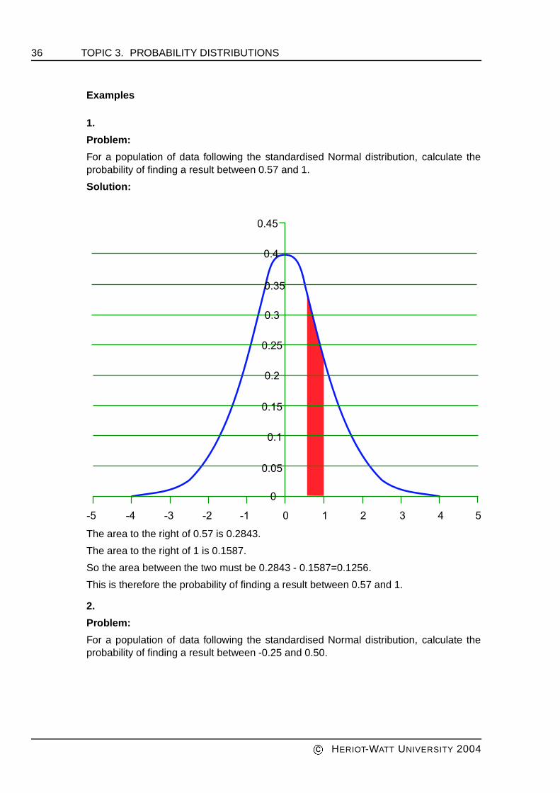
For a population of data following the standardised Normal distribution, calculate theprobability of finding a result between 0.57 and 1.

Solution:

The area to the right of 0.57 is 0.2843.

The area to the right of 1 is 0.1587.

So the area between the two must be 0.2843 - 0.1587=0.1256.

This is therefore the probability of finding a result between 0.57 and 1.

2.

Problem:

For a population of data following the standardised Normal distribution, calculate theprobability of finding a result between -0.25 and 0.50.

c�



Solution:

From tables, the area to the LEFT of-0.25 is 0.4013.

From tables, the area to the RIGHT of 0.50 is 0.3085.

Since the total area under the curve is 1, the area between the two numbers is

1 - (0.4013 + 0.3085)=0.2902.

So the probability of finding a result between -0.25 and 0.50 is 0.2902.

Of course, it is very rare that you will be working with numbers that follow thestandardised normal distribution, but the techniques shown here work equally well aslong as the appropriate results are converted into z-values.

Example

Problem:

For the earlier example of IQ scores which it has been suggested follow a Normaldistribution with mean 100 and standard deviation 15, find the probability that any personchosen at random will have

a) An IQ greater than 110

b) An IQ less than 70

c�



c) An IQ between 70 and 110.

Solution:

The x values (70 and 110 ) must first be converted to z values so that the tables can beused.��

a) z=110 -100/15=0.67

Looking up 0.67 in tables gives 0.2514. This is, therefore, the probability of findingsomeone with an IQ greater than 110.

b) z=70 -100/15=-2.00

Looking up 2.00 in the tables gives 0.0228 (not shown in the sample tables above).By symmetry this is, therefore, the probability of finding someone with an IQ lessthan 70 (in other words, approximately 2%).

c) All the work has been done, so the required probability is 1 -(0.2514 +0.0228)=0.7258.

3.3.6 Upper and Lower Bounds

Sometimes it is useful to START with a probability and then work out related z or xvalues. To do this, the statistical tables can be used in reverse to give upper and lowerbounds as to where, say, 95% of all the data will lie. Take the example of the IQ scoresjust given and use a 95% interval. Now, the area between the two bounded values isknown, but it is the corresponding x values that are not.

c



Since the area to the right of �� is 0.025 (this is because the total area under the curveis 1 and by symmetry the remaining 0.05 must be split in two), statistical tables can beused in reverse to find the appropriate z value of the standardised normal distributionthat gives a probability of 0.025.

Examination of the tables shows this to be 1.96, but for illustrative purposes, this willbe rounded to 2. It was stated earlier that the standardised z distribution measures thenumber of standard deviations away from the mean so the point x2 is therefore 100 +2 � 15=130.

Similarly the value �� can be calculated as 100 - 2 � 15=70

These numbers could also be found by solving the equations�� So � �"! �$#%#�$& �� i.e. �'� �)(+*, , and similarly for �� .Thus it is expected that 95% of the population will have IQ values between 70 and130. The animation below shows the range of values that it would be expected otherpercentages of the population would lie between.

c-



Notice that the range of values increases as a greater percentage of the population isrequired.

In general, for a Normally distributed data set, an empirical rule states that 68% ofthe data elements are within one standard deviation of the mean, 95% are within twostandard deviations, and 99.7% are within three standard deviations. This rule is oftenstated simply as 68-95-99.7.

This type of reasoning can be extended to other distributions that do not have the familiarNormal shape. The Russian mathematician Chebyshev (1821-1894) primarily workedon the theory of prime numbers, although his writings covered a wide range of subjects.One of those subjects was probability and he produced a theorem which states that theproportion of any set of data within K standard deviations of the mean is always at least.0/ 1243 , where K may be any number greater than 1. Note that this theorem applies toany data set, not only Normally distributed ones.

So for K=2, this gives a proportion of.4/ 12 3 , i.e.

.5/ .7678:9<;$678. Thus at least 75% of the

data must always be within two standard deviations of the mean. It has already beenshown that for a Normal distribution the value is 95% (and 75% is clearly less than that).

Similarly, for K=3, it can be seen that.0/�.=>;? 9 .5/�. 6A@�9CBD6A@

. Thus at least 89% ofthe data must always be within three standard deviations of the mean.

Example

Problem:

A machine is designed to fill packets with sugar and the mean value over a long periodof time has been found to be 1kg. The standard deviation has also been measured andthis is given as 0.02kg. What are the upper and lower limits that it would be expected95% of the bags would lie between? Assume the distribution to be Normal.

Solution:

Upper limit : E 3"F 1GIH G ? 9�J. Thus K ? 9 .LNM 8

Lower limit : EO F 1GIH G ? 9 / J. Thus K 1 9 MPL @AQ

cR


3.4. SUMMARY 41

95% of the bags of sugar will lie between 0.96kg and 1.04kg.

Activity

You are given that the mean salary of a UK middle manager is 54.3 thousand pounds,with a standard deviation of 20.1. Assuming a Normal Distribution:

Q3: Calculate the probability that a UK middle manager will earn between 45 and 60thousand pounds.

Q4: Calculate the salary that only 5% of middle managers will earn more than.

3.4 SummaryS Statistics is about collecting, presenting and characterizing data and assists indata analysis and decision making.S Statistics is usually about quantitative data. Often, such data is presented indiagrams.S Basic analysis of data is about the central tendency of data (mean, median, mode),and about the variance of data (variance, standard deviation).S Random variables are functions assigning numerical values to each simple eventof a sample space. We distinguish discrete and continuous random variables.S The probability distribution of a discrete random variable is a function that gives foreach event the probability that the event occurs.S The expected value T�UWVYX is the mean, the standard deviation the square root ofT[Z\UWV�]^T[UWV�X%X`_ba .S Examples of discrete probability distribution are the binomial, geometric,hypergeometric and the Poisson distribution.S For continuous random variables we have to give the cumulative probabilitydistribution.S The relative frequency distribution for a population with continuous randomvariable can be modeled using a density function c'UWVYX (usually a smooth curve)

such that cdUeV�Xgfih and- jkj clU x XnmDVpo)qS Examples of continuous distributions are the uniform distribution, normal

distribution, gamma distribution, the exponential distribution and the Weibulldistribution, of which the normal distribution is the most important.

cr


42 GLOSSARY

Glossary

binomial probability distribution

The binomial probability distributionis given by the formula s�tWuYv wxzyu|{ s~}A��}n��u�w��P��\�\�\� y � where� s is the probability of a success in a single trial, and ��w)��s ;� yis the number of trials; and� u is the number of successes; and� xzyu { is the binomial coefficient given by the number ��}� (n - x)!

binomial random variable

A binomial random variable is a discrete random variable with probabilitydistribution the Binomial distribution.

chi-square distribution

The � 2 (chi-square) probability distribution plays an important role in statistics. Thedistribution is a special case of the gamma distribution for� w�� and � =2

( � is called the number of degrees of freedom).

continuous random variable

A random variable is called continuous if it does not take discrete values.

cumulative distribution of a random variable

The cumulative distribution ��tWu�v of a random variable u is the function ��tWu�v�w��tWu�� uYv .density function

If � is the cumulative distribution of a continuous random variable u then the densityfunction � ( u ) for u is given by�dtWuYv�w��¡ � }(provided that � is differentiable).

expected value of a continuous random variable

The expected value of a continuous random variable u with density function � ( u )is given by ¢ w�£�tWuYv�w|¤¦¥� ¥¨§ �lt § v%© §

expected value of a discrete random variable

For a discrete random variable u with probability distribution sªtWu�v the expectedvalue (or mean) is defined as

c«


GLOSSARY 43

¬®�¯�°W±Y²³|´all x

±�µ·¶�°¸±Y²expected value of a function of a random variable

Theexpected value of ¹ °W±Y² is defined as¯»º ¹ °e±�²$¼' ´all x

¹ °W±Y²�µ%¶�°W±�²exponential density function

The exponential density function is a gamma density function with ½ =1,¾l°W±Y²�À¿AÁgÂÃÄÆÅ x Ç 0

with mean ¬ =Ä

and standard deviation È =Ä

.

gamma random variable

A gamma random variable is a continuous random variable with density functionthe gamma distribution.

geometric probability distribution

The geometric probability distribution is a discrete distribution modeling the eventof a first success after ±¦É�Ê failures. The data for the geometric probabilitydistribution areË P(x) = pqx-1, for x = 1, 2, .....,

where ± is the number of trials until the first success; andËÌ¬ = 1/Í , andË È ÏÎ ÐÍ Ñ .hypergeometric probability distribution

The hypergeometric probability distribution is a discrete distribution that modelssampling without replacement.

Poisson probability distribution

The Poisson probability distribution is a discrete probability distribution. It is oftenused to model frequencies of events.

probability distribution

The probability distribution of a random variable is a table, graph, or formula thatgives the probability ¶ª°W±Y² for each possible value of the random variable ± .

random variable

A random variable is a function taking numerical values which is defined over asample space. Simple random variables could be the temperature of a chemicalprocess or the number of heads when a coin is tossed twice (0,1 or 2). Such arandom variable is called discrete if it only takes countably many values.

cÒ


44 GLOSSARY

standard deviation of a continuous random variable

The standard deviation is defined as Ó = Ô E Õ×Ö x - ØÚÙ·Û"Ü .

standard deviation of a discrete random variable

The variance of a discrete random variable Ý with probability distribution ÞªÖWÝ�Ù isdefined as Ó Û5ß�à Õ×ÖWÝ�á^Ø�Ù`ÛIÜthe standard deviation is defined as Ô à Õ$ÖWÝ[áâØ�Ù`ÛIÜ .

uniform random variable

If we select randomly a number in the interval [ ã>äæå ] then the corresponding randomvariable Ý is called auniform random variable.

cç


ANSWERS: TOPIC 3 45

Answers to questions and activities

3 Probability Distributions

Activity (page 4)

There are two outcomes

A) the company has to pay è 10 000

B) the company doesn’t pay and keeps the premium

p(A) = 0.15

p(B) = 0.85

Assume that the company breaks even and that X is the premium charged.

The Expected Value to the company is 0.15 é (-10 000 + X) + 0.85 é X

To break even this should equal 0

Therefore 0.85X = 1 500 - 0.15X

X = è 1 500

Activity (page 9)

Q1: Binomial distribution. Probability of success, a, is equal to 0.667. This is theprobability of NOT taking school meals regularly. Sample size, n, is equal to 20, so theappropriate formula gives

Q2:

The solution to this uses the fact that we need no more than 5 technicians not to beavailable. This is a binomial probability with p = 0.1 and n = 25.

Required probability is p(0) + p(1) + p(2) + p(3) + p(4) + p(5)

(Probabilities are added because we have a collection of "or" probabilities)

The binomial probability distribution is given by the formulaê�ëWì�í³îðïòñì|ó ê>ôõ�öø÷�ôøù%ìpî�úPù�û\û\û\ù ñThe following values can be calculated easily.

Number not available Probability

0 0.071791 0.199422 0.265893 0.226504 0.138425 0.06459

This gives a total value of 0.96661

cü


46 ANSWERS: TOPIC 3

Activity (page 18)

ýÿþ�� and m=6 (in 2 minutes)

Required probability is p( � 2) = 1- [p(0) + p(1) + p(2)]

Now, ý�þ�� "!$#�%'& ý�þ)(*�� +�-,(�� .(/#�%"0-& ý�þ�!"�� 1!'� �2�� ## � !So p( � 2)=1 - (0.00248 + 0.01487 + 0.04462)=0.93803

Activity (page 28)

The cumulative probability function is given by:3 þ��4��5(76 � � þ*89 �;:For our example, this translates as:3 þ)(��'�<�5(=6 � � þ�>@?�?�?�?ACB�D ? �;E;F AThis calculates as 0.672

So the probability of lasting longer than 10000 hours is 1- 0.672=0.328

The mean (expected value) of the lifetime is:

GIHKJ�LNM (L OExpanding, this gives 9780 P H (1.204).

Using an approximation (tables or computer package), H (1.204) is equal to 0.917.

The mean is therefore 8968 hours.

Activity (page 41)

Q3: The data follows a Normal distribution as follows:

cQ


ANSWERS: TOPIC 3 47

45 54.3 60

Area to the right of 60:

z =x - RS T�U�VXWZY$[.\^]_ V�\a` T V�\ _b

Looking up tables gives a value of 0.3897

Area to the left of 45:

z =x - RS Tc[�YdWZY$[.\^]_ V�\a` T W V�\e[�U

Looking up tables gives a value of 0.3228

The required area is the "bit in the middle" and this is equal to 1 - (0.3897+0.3228). Theanswer is 0.2875.

Q4: Let the point at which the "cut-off" occurs for the top 5% be called t. The areamust be 5% (or 0.05) so using the tables in reverse gives a z value of 1.64.

Therefore, f Thg�i�jk becomes `�\^U$[ Thl i�m)n/o pqsr oetvuxw T _ V�\a`zy{`�\^U$[X|}Y$[.\^] T b"~ \^]So only 5% will earn more than 87.3 thousand.

c�


topic 3 - heriotjphillips/das/dataanalysistopic3.pdf · probability distributions ... 3.3 the...

Documents