topa - 2002 - wavefront reconstruction for the shack-hartmann wavefront sensor

5/9/2018 Topa - 2002 - Wavefront Reconstruction for the Shack-Hartmann Wavefront Sensor - slidepdf.com

http://slidepdf.com/reader/full/topa-2002-wavefront-reconstruction-for-the-shack-hartmann-wavefront-sensor 1/15

SPIE 2002 4769-13 1 of 15 12:21:16, 8/1/02

Wavefront reco nstruc tion for the

Shack-Hartmann w avefront sen sor

Daniel M. Topaa

WaveFr ont Sciences, Inc.

ABSTRACT

The Shack-Hartmann wavefront sensor is powerful tool for optical analysis. A vital step in the data analysis chain

involves reconstructing the wavefront incident upon the lenslet array from hundreds or thousands of slope measure-

ments. We discuss here the basics of reconstruction and the differences in reconstruction for the case of Hartmann and

Shack-Hartmann sensors. Hartmann sensors take point samples of the wavefront but Shack-Hartmann sensors mea-

sure the average slope over small regions. This results in subtle differences in the reconstruction.

Keywords: wavefront reconstruction, direct reconstruction, modal reconstruction, zonal reconstruction, Shack-Hart-

mann

1. INTRODUCTION

A Shack-Hartmann sensor is a simple device. A micro optic array of lenslets dissects an incoming wavefront and cre-

ates a pattern of focal spots on a CCD array. The lenslet array typically contains hundreds or thousands of lenslets,

each on the size scale of a hundred microns. In typical operation, a reference beam is first imaged and the location of

the focal spots is recorded. Then the wavefront of interest is imaged and a second set of focal spot locations is

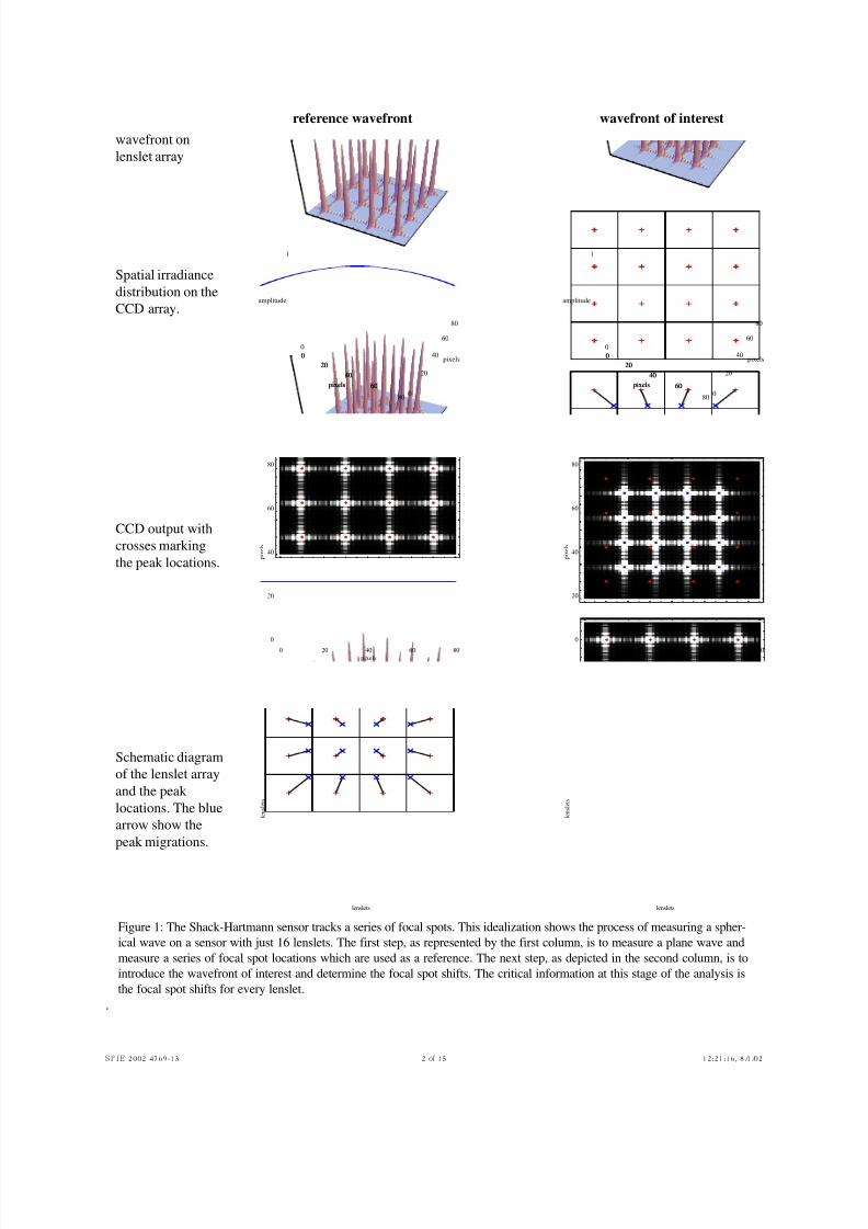
recorded. Figure 1 shows this process graphically. The software then computes the shift in each focal spot. As shown

in another paper in this volume [1], the shift in the focal spot is proportional to the average of the slopes of the wave-

front over the region sampled by the lenslet.

To better understand the main points of this paper, it is worthwhile to discuss the operation in more detail. Usually,

some optical system delivers a wavefront onto the lenslet array which samples the wavefront over the tiny regions of

each lenslet. As pointed out in [1], the lenslets should be much smaller than the wavefront variation, that is, the wave-

front should be isoplanaticb over the sampled region. When the CCD array is in the focal plane of the lenslet array,

each lenslet will create a focal spot on the CCD array. The location of these focal spots is the critical measurement for

it reveals the average of the wavefront slopes across each region. If the wavefront is not isoplanatic, the quality of thefocal spot erodes rapidly and it becomes more difficult to determine the peak location.

This paper will consider the case where the isoplanatic condition is satisfied and where the focal spot shift is con-

sistent with the small angle approximation of Fresnel [2]. In these limits, the focal spot location is exactly propor-

tional to the average of the wavefront slope over the lenslet.

Now the issue becomes how does one take a series of hundreds or thousands of measurements of the average of the

slopes and reconstitute the incident wavefront? This process of taking the measurements and reconstituting the wave-

front incident upon the lenslet array is called reconstruction and is the subject of this paper.

2. WAVEFRONT RECONSTRUCTION

One uses the results of myriad averaged slope measurements to reconstruct the wavefront incident upon the lenslet

array. It is common to hear people describe reconstruction as an integration process. This is malapropos and ironic.

The irony is that Nature has already done the integration for us; as shown below the measured quantity is already an

integrated form of the incident wavefront.

Given a wavefront incident upon a lenslet, what exactly does the sensor measure in the isoplanatic and

small angle limits? It measures the average of the wavefront slopes over each lenslet. So for an integration

domain of , the average of the µ derivative of is given by

a. Phone 505.275.4747; http:/www.wavefrontsciences.com; WaveFront Sciences, Inc., 14810 Central Ave SE, Albu-

querque, NM, 87123-3905. E-mail address: [email protected].

b. Here isoplanatic has the geometric context of being flat “like a plane.” This is different from the context articulated

by Goodman in [2].

ψ x1 x2,( )∂µψ

x1 a b,[ ]∈ x2 c d ,[ ]∈ ψ x1 x2,( )



SPIE 2002 4769-13 2 of 15 12:21:16, 8/1/02

Figure 1: The Shack-Hartmann sensor tracks a series of focal spots. This idealization shows the process of measuring a spher-

ical wave on a sensor with just 16 lenslets. The first step, as represented by the first column, is to measure a plane wave and

measure a series of focal spot locations which are used as a reference. The next step, as depicted in the second column, is to

introduce the wavefront of interest and determine the focal spot shifts. The critical information at this stage of the analysis is

the focal spot shifts for every lenslet.

.

0 20 40 60 80

pixels

0

20

40

60

80

p i x e l s

lenslets

l e n s l e t s

0

20

40

60

80

pixels

0

20

40

60

80

pixels

0

1

amplitude

0

20

40

60pixels

0

20

40

60

80

pixels

0

20

40

60

80

pixels

0

1

amplitude

0

20

40

60pixels

0 20 40 60 80

pixels

0

20

40

60

80

p i x e l s

lenslets

l e n s l e t s

reference wavefront wavefront of interest

wavefront on

lenslet array

Spatial irradiance

distribution on the

CCD array.

CCD output with

crosses marking

the peak locations.

Schematic diagram

of the lenslet array

and the peak

locations. The blue

arrow show the

peak migrations.



SPIE 2002 4769-13 3 of 15 12:21:16, 8/1/02

(1)

where the operator denotes partial differentiation along a line parallel to the µ axis. Defining the antiderivative of

as

, (2)

the average of the slope is written as

(3)

where the domain area has be recast as and ν represents the orthogonal direction. The message

of equation 3 is quite clear: the measurement of the focal spot shift tells us about differences in the antiderivatives

evaluated at the lenslet vertices.

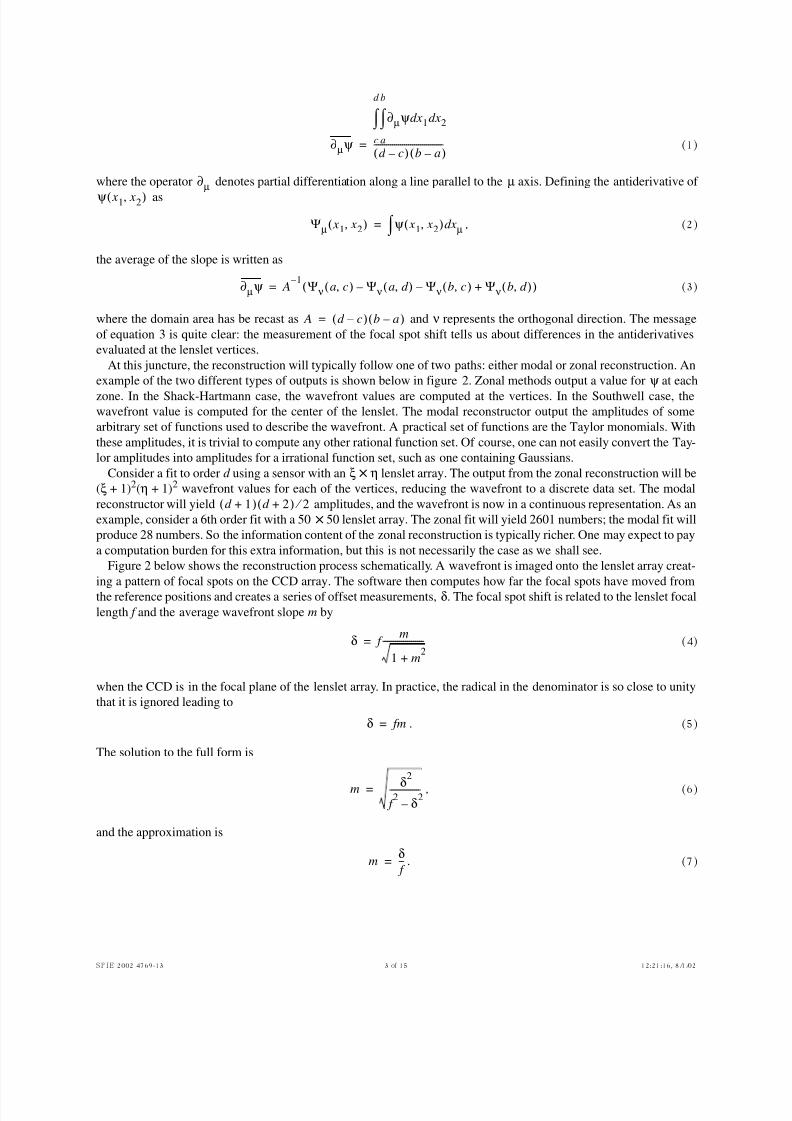
At this juncture, the reconstruction will typically follow one of two paths: either modal or zonal reconstruction. An

example of the two different types of outputs is shown below in figure 2. Zonal methods output a value for ψ at each

zone. In the Shack-Hartmann case, the wavefront values are computed at the vertices. In the Southwell case, the

wavefront value is computed for the center of the lenslet. The modal reconstructor output the amplitudes of some

arbitrary set of functions used to describe the wavefront. A practical set of functions are the Taylor monomials. With

these amplitudes, it is trivial to compute any other rational function set. Of course, one can not easily convert the Tay-

lor amplitudes into amplitudes for a irrational function set, such as one containing Gaussians.

Consider a fit to order d using a sensor with an ξ × η lenslet array. The output from the zonal reconstruction will be

(ξ + 1)2(η + 1)2 wavefront values for each of the vertices, reducing the wavefront to a discrete data set. The modal

reconstructor will yield amplitudes, and the wavefront is now in a continuous representation. As an

example, consider a 6th order fit with a 50 × 50 lenslet array. The zonal fit will yield 2601 numbers; the modal fit will

produce 28 numbers. So the information content of the zonal reconstruction is typically richer. One may expect to pay

a computation burden for this extra information, but this is not necessarily the case as we shall see.

Figure 2 below shows the reconstruction process schematically. A wavefront is imaged onto the lenslet array creat-

ing a pattern of focal spots on the CCD array. The software then computes how far the focal spots have moved fromthe reference positions and creates a series of offset measurements, δ. The focal spot shift is related to the lenslet focal

length f and the average wavefront slope m by

(4)

when the CCD is in the focal plane of the lenslet array. In practice, the radical in the denominator is so close to unity

that it is ignored leading to

. (5)

The solution to the full form is

, (6)

and the approximation is

. (7)

∂µψ

∂µψ xd 1 x2d

a

b

∫ c

d

∫ d c–( ) b a–( )

----------------------------------=

∂µ

ψ x1 x2,( )

Ψµ x1 x2,( ) ψ x1 x2,( ) xµd ∫ =

∂µψ A1– Ψ ν a c,( ) Ψ ν a d ,( )– Ψ ν b c,( ) Ψ ν b d ,( )+–( )=

A d c–( ) b a–( )=

d 1+( ) d 2+( ) 2 ⁄

δ f m

1 m2

+

--------------------=

δ fm=

m δ2

f 2 δ2

–

---------------=

mδ f --=



SPIE 2002 4769-13 4 of 15 12:21:16, 8/1/02

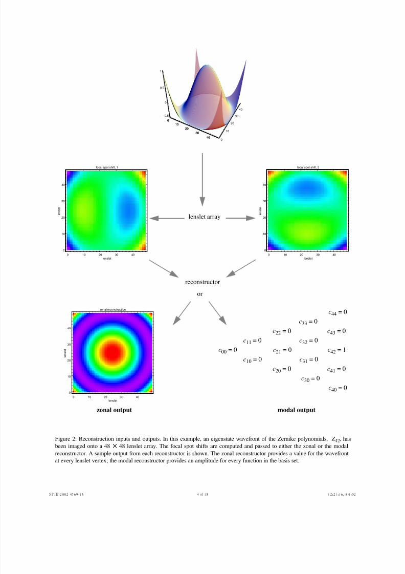
Figure 2: Reconstruction inputs and outputs. In this example, an eigenstate wavefront of the Zernike polynomials, Z 42, has

been imaged onto a 48 × 48 lenslet array. The focal spot shifts are computed and passed to either the zonal or the modal

reconstructor. A sample output from each reconstructor is shown. The zonal reconstructor provides a value for the wavefront

at every lenslet vertex; the modal reconstructor provides an amplitude for every function in the basis set.

0

10

20

30

400

10

20

30

40

-0.5

0

0.5

1

0

10

20

30

40

lenslet array

0 10 20 30 40

lenslet

0

10

20

30

40

l e n s l e t

focal spot shift, 1

0 10 20 30 40

lenslet

0

10

20

30

40

l e n s l e t

focal spot shift, 2

reconstructor

0 10 20 30 40

lenslet

0

10

20

30

40

l e n s l e t

zonal reconstruction

c00 = 0 c21 = 0 c42 = 1

c11 = 0 c32 = 0

c10 = 0 c31 = 0

c20 = 0 c41 = 0

c22 = 0 c43 = 0

c33 = 0

c30 = 0

c44 = 0

c40 = 0

or

zonal output modal output



SPIE 2002 4769-13 5 of 15 12:21:16, 8/1/02

For example, an array with a focal length of 20 mm is imaged onto a CCD array with 24 µm pixels. A shift of two

pixels is measured. The wavefront slope then is 1.2 mr using the approximation in equation 7, and is 1.200000864 mr

using the exact form in equation 6. So for practical purposes, the approximation is adequate for lenslet arrays with

long focal lengths.

The measurement of the focal spot shift δ then is a measurement of the average slope over the lenslet. In the

isoplanatic limit the average slope can be thought of as a tilt. The effect then of a measurement is to reduce the wave-

front into a series of planar patches of the size of each lenslet, with a tilt in each direction corresponding to the focalspot shift in that direction.

To delve deeper into the details of the calculation, we need to introduce some notation. There are a series of N off-

set measurements where is the number of lenslets. Eventually, the linear algebra of zonal reconstruction is

going to force the lenslets to be ordered in a linear fashion. In the interest of expediency, we will use the same order-

ing for both the zonal and the modal cases.

The ordering of the lenslets is completely arbitrary: it can be row major, column major or even random. The posi-

tion vector p describes the linear ordering of the addresses. A sample p vector is

(8)

where the address pairs (u, v) denote rows and columns. On an array, the address (u, v) would be at position

in the p vector. The reverse look-up procedure is a bit more involved. It is simple to compute, but in

practice, it is convenient to construct a lookup table q which is really an matrix. A sample q matrix is shown

below

. (9)

3. MODAL RECONSTRUCTION

Equation 3 has already paved the road for modal reconstruction. Before beginning with the details of reconstruction,

it is helpful to define the box operator for an arbitrary function over the domain , . This

operator combines the values of a function at the domain corners in the following way:

. (10)

Having seen the box operator in an explicit form, we will now generalize its formulation. Consider the rectangular

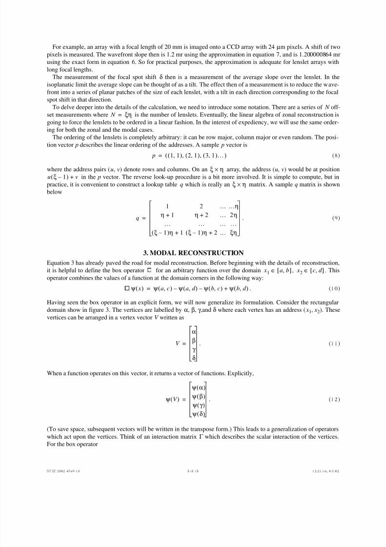
domain show in figure 3. The vertices are labelled by α, β, γ ,and δ where each vertex has an address ( x1, x2). These

vertices can be arranged in a vertex vector V written as

. (11)

When a function operates on this vector, it returns a vector of functions. Explicitly,

. (12)

(To save space, subsequent vectors will be written in the transpose form.) This leads to a generalization of operators

which act upon the vertices. Think of an interaction matrix Γ which describes the scalar interaction of the vertices.

For the box operator

N ξη=

p 1 1,( ) 2 1,( ) 3 1,( )…, ,( )=

ξ η×u ξ 1–( ) v+

ξ η×

q

1 2 … …ηη 1+ η 2+ … 2η

… … … …ξ 1–( )η 1+ ξ 1–( )η 2+ … ξη

=

x1 a b,[ ]∈ x2 c d ,[ ]∈

ψ x( ) ψ a c,( ) ψ a d ,( )– ψ b c,( )– ψ b d ,( )+=

V

αβγ δ

=

ψ V ( )

ψ α( )ψ β( )ψ γ ( )ψ δ( )

=



SPIE 2002 4769-13 6 of 15 12:21:16, 8/1/02

Figure 3: The vertices of a lenslet. Here the vertex points are labelled with the Greek letters α through δ. Each of these letters

is really an address pair. The indexing of the vertices is tied to the indexing for the lenslet. If this is lenslet (u, v), then α is ver-

tex (u-1, v-1); β is (u, v-1), γ is (u, v), and δ is (u-1, v).

(13)

and we can now write

. (14)

With this box operator, the average of the µ slope mµ over the lenslet at address pi is expressed as

(15)

In this case is the predicted value. But the actual measurement is of . To find the wavefront which best

describes the measurements, one simply needs to minimize the merit function

(16)

where σi represents an error estimate. However, since these errors do not depend upon the amplitudes, they can be

treated as weighting factors and are withheld from explicit evaluation.

All that remains now is to chose a set of basis functions. This set should be complete. Orthogonal sets are attrac-

tive, but often involve unneeded overhead as shown in [3]. The set we will choose is the basis set for all rational func-

tions: the Taylor monomials. These monomials are given by

(17)

and the wavefront described as a d th order expansion would be written as

. (18)

We specify this set because it contains all the information needed to construct the functions of all other rational basis

sets, such as the polynomials of Zernike or Legendre. It is easiest to work in the Taylor basis and then use an affine

transformation on the Taylor amplitudes to compute the amplitudes in the other bases. These transformations matri-

ces are written in terms of integers, so there is no loss of precision.

Also, the Taylor basis far easier to work with. Consider the case of the antiderivatives. They can be written to arbi-

trary order as

α β

γ δ

Γ B

1– 0 0 0

0 1 0 0

0 0 1– 0

0 0 0 1

=

ψ x( ) Γ Bψ V ( )=

mµ pi, A

1– Ψ ν V pi( )=

mµ pi, δ pi

µ

χ

2δ pi

µ f

A--- Ψ ν pi

,– 2

σi2

--------------------------------------------

i 1=

N

∑µ 1=

2

∑=

T i j j,–

x1 x2,( ) x1

i j– x2

j=

ψ x1 x2,( ) ai j j,– x1i j– x2

j

j 0=

i

∑i 0=

d

∑=



SPIE 2002 4769-13 7 of 15 12:21:16, 8/1/02

, (19)

and

(20)

By comparison, writing out the two antiderivatives for each of the 66 Zernike polynomials through 10th order would

fill several pages.

Anyway, the following analysis does not depend upon the basis set. The minimization of the merit function pro-

ceeds in the canonical way: the derivatives with respect to each amplitude are set to zero,

. (21)

This will generate a series of linear equations to solve. Since this is a linear least squares fit,

we expect to find a direct solution. All that remains are some linear algebra details unique to the basis set chosen. In

the interest of brevity, we will focus to the issue of zonal reconstruction.

4. ZONAL RECONSTRUCTION

We now consider the problem of zonal reconstruction for the Shack-Hartmann sensor. Here too we start with equation

3 and derive the merit function ∆ (which is χ2 without the σi terms):

(22)

There is a problem with the antiderivative terms. They are quite unwelcome for a zonal fit because it would require

discrete differentiation to recover to wavefront values. It is better to recast ∆ to explicitly compute the wavefront val-

ues. So we turn our attention to the task of eliminating the antiderivatives. We begin with a close examination of

equation 1. Note that in one dimension, the average value of the derivative of a function g(x) over the linear domain

is trivial to compute:

. (23)

The trouble arises when we average in the orthogonal direction. This is what creates the troublesome antiderivatives.

So in lieu of an exact average over an area, we use an approximation by computing the average of equation 23 evalu-

ated at the endpoints of the domain . This process is

(24)

Defining the vertex interaction matrix Γ 1 as

(25)

and the lenslet width vector h as

T 1i j j,–

x1 x2,( ) 1

i j– 1+------------------ x1

i j– 1+ x2

j=

T 2i j j,–

x1 x2,( ) 1

j 1+----------- x1

i j– x2

j 1+=

∂ai j j,–

χ20=

n d 1+( ) d 2+( ) 2 ⁄ =

∆ δ pi

µ f

A--- Ψ ν pi,–

2

i 1=

N

∑µ 1=

2

∑=

x1 a b,[ ]∈

∂1g x1 x2,( )linear g b x2,( ) g a x2,( )–

b a–---------------------------------------------=

x2 c d ,[ ]∈

∂1g x1 x2,( ) 1

2 b a–( )-------------------- g b x2,( ) g a x2,( )–( )

x2 c=g b x2,( ) g a x2,( )–( )

x2 d =+≈

1

2 b a–( )-------------------- g b c,( ) g a c,( )– g b d ,( ) g a d ,( )–+( )=

Γ 1

1– 0 0 0

0 1 0 0

0 0 1 0

0 0 0 1–

=



SPIE 2002 4769-13 8 of 15 12:21:16, 8/1/02

(26)

allows us to write the approximation as

(27)

where the vertex vector V is given by

. (28)

Similar machinations yield the result

(29)

where the interaction matrix is

. (30)

The approximations in equations 27 and 29 are now the surrogate values for the exact form of the averaged slopes.

The appendix explores the validity of these approximations and shows that it many cases it is exact.

At last we can replace equation 22 and pose the new merit function as

, (31)

liberating us from the problems of having to deal with antiderivatives. The minimization is routine. The quantitiesbeing varied are the wavefront values at each vertex. All the derivatives with respect to the wavefront values at the

vertices are set equal to zero:

. (32)

The vector p now indexes the vertices, not the lenslets.

The net effect is a series of linear equations that look like this (after the simplification h1 = h2 = h):

(33)

where s is an alignment spinor given by

. (34)

hb a–

d c–=

∂1g x1 x2,( ) 1

2h1

--------Γ 1g V ( )≈

V T

a c,( ) b c,( ) b d ,( ) a d ,( ), , ,( )=

∂2g x1 x2,( ) 1

2h2

--------Γ 2g V ( )≈

Γ 2

1– 0 0 0

0 1– 0 0

0 0 1 0

0 0 0 1

=

∆ δ pi

µ f

2hµ---------Γ µψ V pi

( )– 2

i 1=

N

∑µ 1=

2

∑=

∂ψ p

i

∆ 0=

4ψ u v, ψ

u 1 v 1–,–– ψ u 1+ v 1–,– ψ

u 1+ v, 1+– ψ u 1– v, 1+–

h

f --- s1

T δ u v,( ) s2T δ u 1 v,+( ) s2

T δ u v, 1+( )– s1T δ u 1 v 1+,+( )–+( )=

s

1

1

1

1–

=



SPIE 2002 4769-13 9 of 15 12:21:16, 8/1/02

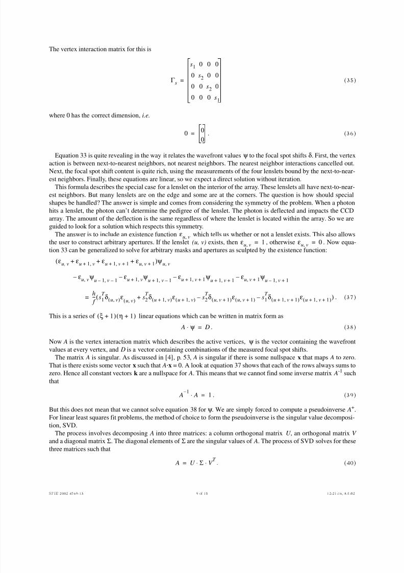
The vertex interaction matrix for this is

(35)

where 0 has the correct dimension, i.e.

. (36)

Equation 33 is quite revealing in the way it relates the wavefront values ψ to the focal spot shifts δ. First, the vertex

action is between next-to-nearest neighbors, not nearest neighbors. The nearest neighbor interactions cancelled out.

Next, the focal spot shift content is quite rich, using the measurements of the four lenslets bound by the next-to-near-

est neighbors. Finally, these equations are linear, so we expect a direct solution without iteration.

This formula describes the special case for a lenslet on the interior of the array. These lenslets all have next-to-near-

est neighbors. But many lenslets are on the edge and some are at the corners. The question is how should special

shapes be handled? The answer is simple and comes from considering the symmetry of the problem. When a photon

hits a lenslet, the photon can’t determine the pedigree of the lenslet. The photon is deflected and impacts the CCD

array. The amount of the deflection is the same regardless of where the lenslet is located within the array. So we are

guided to look for a solution which respects this symmetry.

The answer is to include an existence function which tells us whether or not a lenslet exists. This also allows

the user to construct arbitrary apertures. If the lenslet (u, v) exists, then , otherwise . Now equa-

tion 33 can be generalized to solve for arbitrary masks and apertures as sculpted by the existence function:

. (37)

This is a series of linear equations which can be written in matrix form as

. (38)

Now A is the vertex interaction matrix which describes the active vertices, ψ is the vector containing the wavefront

values at every vertex, and D is a vector containing combinations of the measured focal spot shifts.

The matrix A is singular. As discussed in [4], p. 53, A is singular if there is some nullspace x that maps A to zero.

That is there exists some vector x such that A·x = 0. A look at equation 37 shows that each of the rows always sums to

zero. Hence all constant vectors k are a nullspace for A. This means that we cannot find some inverse matrix A-1 such

that

. (39)

But this does not mean that we cannot solve equation 38 for ψ . We are simply forced to compute a pseudoinverse A+.

For linear least squares fit problems, the method of choice to form the pseudoinverse is the singular value decomposi-

tion, SVD.

The process involves decomposing A into three matrices: a column orthogonal matrix U , an orthogonal matrix V

and a diagonal matrix Σ. The diagonal elements of Σ are the singular values of A. The process of SVD solves for these

three matrices such that

. (40)

Γ s

s1 0 0 0

0 s2 0 0

0 0 s2 0

0 0 0 s1

=

00

0=

εu v,εu v, 1= εu v, 0=

εu v, ε

u 1+ v, εu 1+ v, 1+ ε

u v, 1++ + +( )ψ u v,

εu v, ψ u 1 v 1–,–

– εu 1+ v, ψ u 1+ v 1–,– εu 1+ v, 1+ ψ

u 1+ v, 1+– εu v, 1+ ψ

u 1– v, 1+–

h

f ---

s1

T

δ u v,( )ε u v,( ) s2

T

δ u 1 v,+( )ε u 1 v,+( ) s2

T

δ u v, 1+( )ε u v, 1+( )– s1

T

δ u 1 v 1+,+( )ε u 1 v 1+,+( )–+( )=

ξ 1+( ) η 1+( )

A ψ ⋅ D=

A1–

A⋅ 1=

A U Σ V T ⋅ ⋅=

http://-/?-

http://-/?-

http://-/?-

http://-/?-



SPIE 2002 4769-13 10 of 15 12:21:16, 8/1/02

The pseudoinverse is now given by

. (41)

The entire process of reconstruction distills down to the matrix multiplication.

. (42)

This is a very powerful statement for it shows how most of the computation can be done in advance. For a fixed lens-

let geometry, the matrix A+ can be precomputed and stored. It does not need to be created during the measurement

process.

There is some fine print however. First of all, A+ is very large. For a 64 × 64 lenslet array, A+ has 654 elements

which is about 136 MB of data. Next, the computation may take hours. So it behooves the user find ways to avoid

recomputation when the aperture changes. Some strategies involve storing A+ for many common apertures such as a

series of circular masks. Another strategy is to pad the data. Consider A+ for a full aperture. All lenslets are active.

Then for some reason a cluster of three lenslets is excluded from the data. A good idea is to use the same A+ matrix

and just pad the data in the excluded regions with some form of average data from the neighbors and exclude these

vertices in the final result.

So in closing, zonal reconstruction starts with the antiderivatives and uses matrix multiplication to compute the

wavefront values at each vertex in one step.

5. SOUTHWELL REDUX

In a very influential paper published in 1980 [5], W. Southwell set forth what has become the standard method for

wavefront reconstruction. The paper very clearly describes his reconstructor and is worth reading. Surprisingly

though, Southwell solved his linear equations using successive overrelaxation (SOR). While SOR is an extremely

valuable method, we feel that SVD is usually the better choice.

We will compare the philosophical differences between the two reconstructors in the following section. Here we

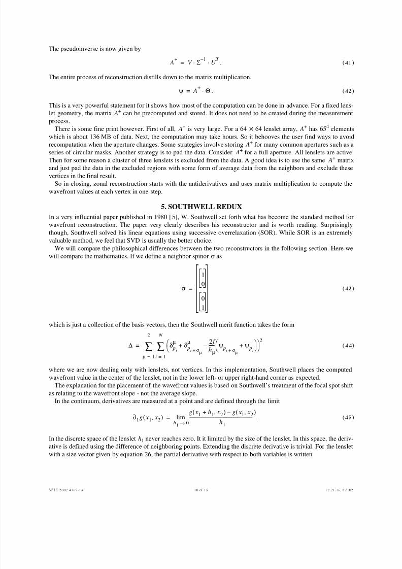
will compare the mathematics. If we define a neighbor spinor σ as

(43)

which is just a collection of the basis vectors, then the Southwell merit function takes the form

(44)

where we are now dealing only with lenslets, not vertices. In this implementation, Southwell places the computed

wavefront value in the center of the lenslet, not in the lower left- or upper right-hand corner as expected.

The explanation for the placement of the wavefront values is based on Southwell’s treatment of the focal spot shift

as relating to the wavefront slope - not the average slope.

In the continuum, derivatives are measured at a point and are defined through the limit

. (45)

In the discrete space of the lenslet h1 never reaches zero. It it limited by the size of the lenslet. In this space, the deriv-

ative is defined using the difference of neighboring points. Extending the discrete derivative is trivial. For the lenslet

with a size vector given by equation 26, the partial derivative with respect to both variables is written

A+

V Σ 1–U

T ⋅ ⋅=

ψ A+ Θ⋅=

σ

1

0

01

=

∆ δ pi

µ δ pi σµ+

µ 2 f

hµ----- ψ pi σµ+

ψ pi+

–+ 2

i 1=

N

∑µ 1=

2

∑=

∂1g x1 x2,( )g x1 h1 x2,+( ) g x1 x2,( )–

h1

-------------------------------------------------------------h

10→

lim=



SPIE 2002 4769-13 11 of 15 12:21:16, 8/1/02

. (46)

In light of this equation 3 can be viewed as

. (47)

This seems to suggest that if the measurements are treated as slope measurements, and not averaged slope measure-

ments, then the wavefront values should be placed in the lower left-hand corner of the lenslet or the upper right-hand

corner depending on whether the limit is approaching zero from the right or the left.

Returning to the Southwell minimization problem, we proceed as before. The parameters being computed are the

wavefront values at the center of the lenslet and we vary ∆ with respect to these values and set the derivative equal to

zero:

. (48)

For a ξ × η lenslet array with h1 = h2 = h, this leads to linear equations of the form

. (49)

(The existence function has been eliminated to facilitate comparison). So the Southwell interaction involves nearest-

neighbor lenslets and uses only four measured values.

As before we can write a matrix expression just like equation 42. The lenslet interaction matrix A here is singular

and we again resort to SVD. This allows for a direct solution and in many cases, we may precompute A+. Both meth-

ods will execute in equivalent times.

6. PHILOSOPHICAL DIFFERENCES

It is time to step away from the mathematical details and talk about the differences between the two reconstruction

strategies. The new method strictly adheres to the assumptions of Shack-Hartmann operation. It treats the measure-

ments as being extended quantities, not point measurements. This is why the wavefront value cannot be placed at a

single point. In this model, we are only permitted to make statements about the values at the vertices. Subsequent

mathematics are then dictated.In Southwell’s venerable model, he assumes that the difference between the wavefront values in adjacent lenslets is

related to the average slope across those two lenslets. One thing that seemed unusual was that the average of the two

measurements was not placed on the boundary between the two lenslets. Regardless, the Southwell model looks at a

lenslet, it averages the δ1 measurement with the lenslet in the 1 direction and averages the δ2 measurement with the

lenslet in the 2 direction.

Southwell’s model mixes information from lenslets immediately. The new model assumes that the measurement of

a focal spot shift reveals information about the differences in wavefront values at the vertices. However, the neighbor-

ing lenslets each share two vertices. So the competing values for the shared vertices are adjudicated by the least

squares fit. So clearly, the new model is also sharing information between lenslets, but not until the least squares fit.

Perhaps the most obvious shortcoming with an immediate averaging is that small features of the order of a lenslet

will be diminished. In day to day practice, this will probably not be noticed by most users. Only those requiring

exquisite detail resolution would be driven towards the new method.

Another interesting difference between the two is in the wavefront value interaction. The Southwell equations bal-ance the wavefront values with the four nearest neighbors. In the new method, the nearest neighbors interactions can-

cel out, and the surviving interaction is between the next-to-nearest neighbor vertices. This is shown schematically in

figure 4 below. So it is not that the nearest neighbor interaction is avoided, it is just that they exactly cancel out.

Finally we note that the measurement content of the Θ matrix is richer in the new model. Southwell blends together

four measurements, and the new model blends eight.

In summary, both methods have a comparable run time and the memory requirements are virtually identical. They

are both direct methods and both allow for arbitrary aperture shapes. The primary difference seems to be an improve-

ment in resolution of fine details. Comparisons in the way the two models handle noise need to be done yet.

∂1 2, g x1 x2,( )g x1 x2,( ) g x1 h1+ x2 h2+,( ) g x1 h1+ x2,( )– g x1 x2 h2+,( )–+

h1h2

---------------------------------------------------------------------------------------------------------------------------------------------------------≈

∂1 2, Ψµ x1 x2,( ) ∂υψ x1 x2,( )≈

∂ψ pi

∆ 0=

N ξη=

4ψ u v, ψ u 1 v,–– ψ u 1+ v,– ψ u v, 1+– ψ u v, 1––h

2 f ----- δ u 1 v,–( )

1 δ u 1 v,+( )1 δ u v 1–,( )

2– δ u v 1+,( )

2–+( )=



SPIE 2002 4769-13 12 of 15 12:21:16, 8/1/02

(a) (b)

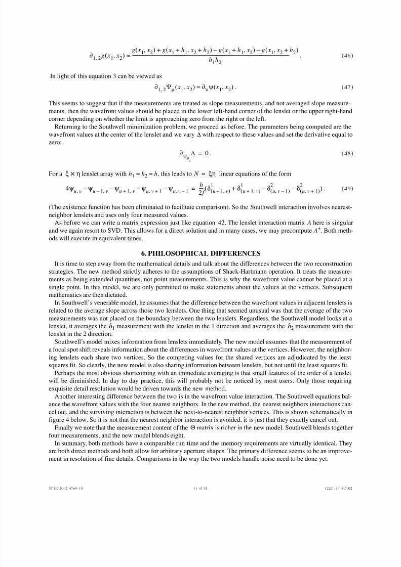
Figure 4: Comparing the interactions of the wavefront values in the least squares fit. In the Southwell model depicted in (a),

the wavefront value is balanced between a central lenslet (marked in red) and the four nearest neighbors. This can be seen in

equation 49. In the new model shown in (b), the wavefront value is balanced between a central vertex and the four next -to-

nearest neighbors and the nearest neighbor interactions exactly cancel. The resultant interaction is specified in equation 33.

7. COMPARISON OF THE TWO METHODSThis section evaluates some sample wavefront that we put into both models and give the reader a visual comparison

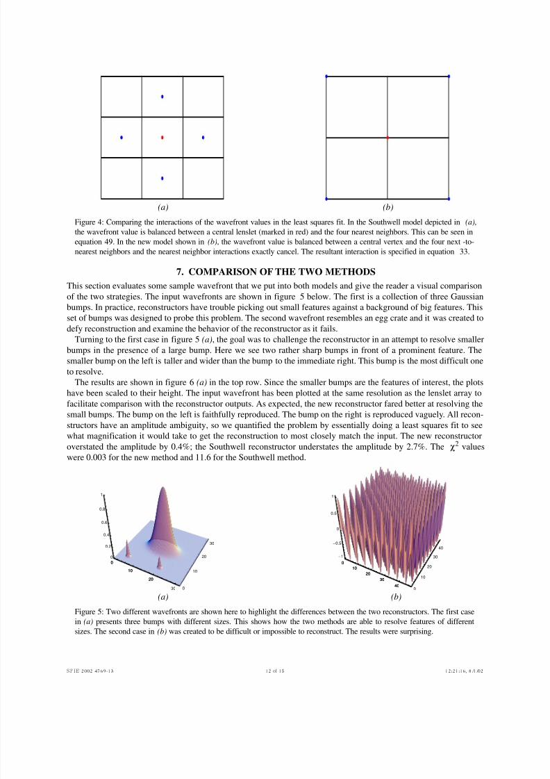
of the two strategies. The input wavefronts are shown in figure 5 below. The first is a collection of three Gaussian

bumps. In practice, reconstructors have trouble picking out small features against a background of big features. This

set of bumps was designed to probe this problem. The second wavefront resembles an egg crate and it was created to

defy reconstruction and examine the behavior of the reconstructor as it fails.

Turning to the first case in figure 5 (a), the goal was to challenge the reconstructor in an attempt to resolve smaller

bumps in the presence of a large bump. Here we see two rather sharp bumps in front of a prominent feature. The

smaller bump on the left is taller and wider than the bump to the immediate right. This bump is the most difficult one

to resolve.

The results are shown in figure 6 (a) in the top row. Since the smaller bumps are the features of interest, the plots

have been scaled to their height. The input wavefront has been plotted at the same resolution as the lenslet array to

facilitate comparison with the reconstructor outputs. As expected, the new reconstructor fared better at resolving thesmall bumps. The bump on the left is faithfully reproduced. The bump on the right is reproduced vaguely. All recon-

structors have an amplitude ambiguity, so we quantified the problem by essentially doing a least squares fit to see

what magnification it would take to get the reconstruction to most closely match the input. The new reconstructor

overstated the amplitude by 0.4%; the Southwell reconstructor understates the amplitude by 2.7%. The χ2 values

were 0.003 for the new method and 11.6 for the Southwell method.

(a) (b)

Figure 5: Two different wavefronts are shown here to highlight the differences between the two reconstructors. The first case

in (a) presents three bumps with different sizes. This shows how the two methods are able to resolve features of different

sizes. The second case in (b) was created to be difficult or impossible to reconstruct. The results were surprising.

0

10

20

30 0

10

20

30

0

0.2

0.4

0.6

0.8

1

0

10

20

0

10

20

30

400

10

20

30

40

-1

-0.5

0

0.5

1

0

10

20

30

40

http://-/?-

http://-/?-

http://-/?-

http://-/?-

http://-/?-

http://-/?-



SPIE 2002 4769-13 13 of 15 12:21:16, 8/1/02

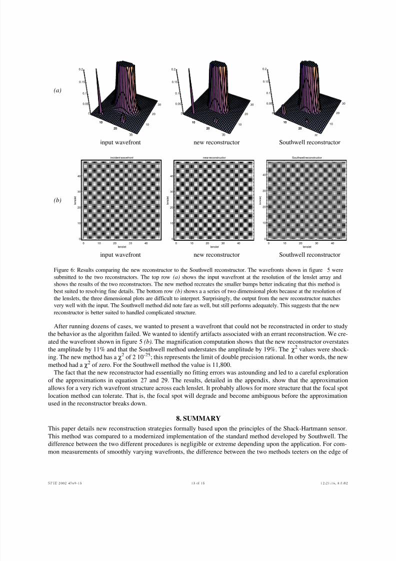
Figure 6: Results comparing the new reconstructor to the Southwell reconstructor. The wavefronts shown in figure 5 were

submitted to the two reconstructors. The top row (a) shows the input wavefront at the resolution of the lenslet array and

shows the results of the two reconstructors. The new method recreates the smaller bumps better indicating that this method is

best suited to resolving fine details. The bottom row (b) shows a a series of two dimensional plots because at the resolution of the lenslets, the three dimensional plots are difficult to interpret. Surprisingly, the output from the new reconstructor matches

very well with the input. The Southwell method did note fare as well, but still performs adequately. This suggests that the new

reconstructor is better suited to handled complicated structure.

After running dozens of cases, we wanted to present a wavefront that could not be reconstructed in order to study

the behavior as the algorithm failed. We wanted to identify artifacts associated with an errant reconstruction. We cre-

ated the wavefront shown in figure 5 (b). The magnification computation shows that the new reconstructor overstates

the amplitude by 11% and that the Southwell method understates the amplitude by 19%. The χ2 values were shock-

ing. The new method has a χ2 of 2 10-25; this represents the limit of double precision rational. In other words, the new

method had a χ2 of zero. For the Southwell method the value is 11,800.

The fact that the new reconstructor had essentially no fitting errors was astounding and led to a careful exploration

of the approximations in equation 27 and 29. The results, detailed in the appendix, show that the approximation

allows for a very rich wavefront structure across each lenslet. It probably allows for more structure that the focal spot

location method can tolerate. That is, the focal spot will degrade and become ambiguous before the approximation

used in the reconstructor breaks down.

8. SUMMARY

This paper details new reconstruction strategies formally based upon the principles of the Shack-Hartmann sensor.

This method was compared to a modernized implementation of the standard method developed by Southwell. The

difference between the two different procedures is negligible or extreme depending upon the application. For com-

mon measurements of smoothly varying wavefronts, the difference between the two methods teeters on the edge of

10

20

30

10

20

30

0

0.05

0.1

0.15

0.2

10

20

10

20

30

10

20

30

0

0.05

0.1

0.15

0.2

10

20

10

20

30

10

20

30

0

0.05

0.1

0.15

0.2

10

20

0 10 20 30 40

lenslet

0

10

20

30

40

l e n s l e t

new reconstructor

0 10 20 30 40

lenslet

0

10

20

30

40

l e n s l e t

incident wavefront

0 10 20 30 40

lenslet

0

10

20

30

40

l e n s l e t

Southwell reconstructor

(a)

(b)

input wavefront new reconstructor Southwell reconstructor

input wavefront new reconstructor Southwell reconstructor

http://-/?-

http://-/?-

http://-/?-

http://-/?-



SPIE 2002 4769-13 14 of 15 12:21:16, 8/1/02

imperceptible. However if the wavefront of interest is richly structured or finely detailed, then the new method is a

substantial improvement.

APPENDIX: VALIDATING THE APPROXIMATION

The results on the egg crate reconstruction (figure 5 (b)) were startling. After all, the wavefront was designed to break

the reconstructor, yet the χ2

was zero to the limit of machine precision. This inspired a detailed look at the approxi-mation used in equations 27 and 29. This section documents the investigation.

To recap, the merit function (equation 22) for Shack-Hartmann sensors involves antiderivatives, which are unwel-

come in a zonal reconstruction. An approximation was used to bypass the nettlesome antiderivatives and formulate a

merit function based on the wavefront values. The approximation is contained in the two equations

. (50)

We start by forming the sum and the difference of the two equations represented above. Remembering that the

domain is , we find that

, (51)

and

. (52)

At this point we need to be more specific about . We can represent this function as a Taylor series. This is

not because we champion the use of the Taylor monomials in modal reconstruction; it is because any piecewise con-

tinuous function can be described exactly by an infinite series of the monomials. We now write

. (53)

When this expansion is substituted into equations 51 and 52, we see

, (54)

and

. (55)

Using the identity

1

2h ν---------Γ µψ V ( ) 1

hµh ν------------Γ BΨ ν V ( )≈

x1 a b,[ ]∈ x2 c d ,[ ]∈

ψ b d ,( ) ψ a c,( )–1

h2

----- Ψ2 x1 x2,( ) 1

h1

----- Ψ1 x1 x2,( )+=

ψ b c,( ) ψ a d ,( )–1

h2

----- Ψ2 x1 x2,( ) 1

h1

----- Ψ1 x1 x2,( )–=

ψ x1 x2,( )

ψ x1 x2,( ) αi j j,– x

i j– y

j

j 0=

i

∑i 0=

∞

∑=

αi j j,– bi j–

d j

ai j–

c j

–( )

j 0=

i

∑i 0=

d

∑

1

h2

-----α

i j j,–

j 1+--------------- b

i j–a

i j––( ) d

j 1+c j 1+

–( )

j 0=

i

∑i 0=

d

∑1

h1

-----α

i j j,–

i j– 1+------------------ b

i j– 1+a

i j– 1+–( ) d

jc j

–( )

j 0=

i

∑i 0=

d

∑+=

αi j j,– bi j– c j ai j– d j–( )

j 0=

i

∑i 0=

d

∑

1

h2

-----αi j j,–

j 1+--------------- b

i j–a

i j––( ) d

j 1+c j 1+

–( )

j 0=

i

∑i 0=

d

∑1

h1

-----αi j j,–

i j–--------------- b

i j– 1+a

i j– 1+–( ) d

jc j

–( )

j 0=

i

∑i 0=

d

∑+=

http://-/?-

http://-/?-



SPIE 2002 4769-13 15 of 15 12:21:16, 8/1/02

(56)

one can show that the approximations in equation 50 are exact whenever the wavefront over the lenslet has a structure

like

. (57)

This allows for an incredible amount of structure over the lenslet. For example, any separable function

(58)

will be handled exactly; in other words, there is an exact solution and it is described by equation 42. Or any separable

function with the lowest order torsion term, for example

. (59)

The egg crate wavefront in figure 5(b) is

(60)

which is exactly the form of equation 58.

ACKNOWLEDGMENTS

We are grateful to D. McMahon and C. Burak for many enlightening discussions. The editorial help of J. Copland, G.

Pankretz, P. Pulaski, and P. Riera was quite helpful.

REFERENCES

1. Topa, D.M., Optimized methods for focal spot location using center of mass algorithms, SPIE Vol. 4769, 2002.

2. Goodman, J.W., Introduction to Fourier Optics 2e, McGraw-Hill, 1988, p. 66.

3. Riera, P.R., Pankretz, G.S., and Topa, D.M., Efficient computation with special functions like the circle polynomials

of Zernike, SPIE Vol. 4769, 2002.

4. Press, W.H., Teukolsky, S.A., Vetterling, W.T., and Flannery, B.P., Numerical Recipes in FORTRAN 2e, Cam-

bridge, 1992.

5. Southwell, W.H., Wave-front estimation from wave-front slope measurements, J. Opt. Soc. Am., 70(8), p.988, 1980.

sk 1+

t k 1+

–

s t –----------------------------- s

k i–t i

i 0=

k

∑=

ψ x1 x2,( ) α00 α11 x1 x2 αi0 x1

i α0i x2

i

i 1=

∞

∑+

i 1=

∞

∑+ +=

ψ x1 x2,( ) X x1( )Y x2( )=

ψ x1 x2,( ) X x1( )Y x2( ) kx1 x2+=

ψ x1 x2,( ) k 1 x1( ) k 2 x2( )cossin=

http://-/?-

http://-/?-

topa - 2002 - wavefront reconstruction for the shack-hartmann wavefront sensor

Documents