top-k with diversity-m data retrieval in wireless sensor
TRANSCRIPT

Scholars' Mine Scholars' Mine
Masters Theses Student Theses and Dissertations
Fall 2014
Top-K with diversity-M data retrieval in wireless sensor networks Top-K with diversity-M data retrieval in wireless sensor networks
Kiran Kumar Puram
Follow this and additional works at: https://scholarsmine.mst.edu/masters_theses
Part of the Computer Sciences Commons
Department: Department:
Recommended Citation Recommended Citation Puram, Kiran Kumar, "Top-K with diversity-M data retrieval in wireless sensor networks" (2014). Masters Theses. 7338. https://scholarsmine.mst.edu/masters_theses/7338
This thesis is brought to you by Scholars' Mine, a service of the Missouri S&T Library and Learning Resources. This work is protected by U. S. Copyright Law. Unauthorized use including reproduction for redistribution requires the permission of the copyright holder. For more information, please contact [email protected].


TOP-K WITH DIVERSITY-M DATA RETRIEVAL IN
WIRELESS SENSOR NETWORKS
by
KIRAN KUMAR PURAM
A THESIS
Presented to the Faculty of the Graduate School of the
MISSOURI UNIVERSITY OF SCIENCE AND TECHNOLOGY
In Partial Fulfillment of the Requirements for the Degree
MASTER OF SCIENCE IN COMPUTER SCIENCE
2014
Approved by
Sanjay Kumar Madria, Advisor
Sriram Chellappan
Maciej Zawodniok

iii
ABSTRACT
Wireless Sensor Network is a network of a few to several thousand sensors
deployed over an area to sense data and report that data back to the base station. There
are many applications of wireless sensor networks including environment monitoring,
wildlife tracking, troop tracking etc. The deployed sensors have many constraints like
limited battery, limited memory and very little processing capacity. These constraints
show direct effect on the network life time.
In many applications of Wireless Sensor Networks, such as monitoring chemical
leak, the user is not interested in all the data points from the entire region, but may want
only top-k values. Moreover, a user may also be interested in getting top-k with diversity-
m, Top (k,m), that is, top-k data should come from m different sub-regions (i.e., clusters).
In this thesis, thus, we have considered the problem of continuous top-k query with
diversity-m, i.e. we want to find the k highest values from at least m different clusters
over a period of time in a wireless sensor network. In this context, we introduce an
energy efficient scheme called Top (k,m). Our scheme is to utilize the Gaussian's
probability function in estimating the probability of a sensor node value being in the final
top-k set. Based on the probability, the node decides whether to forward data values to
the base station or not. Moreover, we also make sure that top-k data items are coming
from at least m-clusters, which is very helpful in monitoring applications. We have
examined the performance of our scheme with respect to EXTOK and Grid approaches in
terms of communication, energy usage and network life time.

iv
ACKNOWLEDGEMENTS
I would like to express my gratitude to all those who have helped me with this
research. First, I would like to thank my advisor Dr. Sanjay Kumar Madria who gave me
the opportunity to work on this research topic. I am grateful to him for the advice and
guidance he gave me throughout my Master’s program. Secondly, I would like to thank
Dr. Sriram Chellappan and Dr. Maciej Jan Zawodniok for being part of my thesis
committee and taking time to review this work.
A special thanks to all my friends for understanding and standing by me during
my tough times. Finally, I would like to dedicate this work to my parents and my brother
for their emotional support and unconditional love and sacrifices.

v
TABLE OF CONTENTS
Page
ABSTRACT ....................................................................................................................... iii
ACKNOWLEDGEMENTS ............................................................................................... iv
LIST OF ILLUSTRATIONS ............................................................................................. vi
LIST OF TABLES ........................................................................................................... viii
SECTION
1. INTRODUCTION ................................................................................................1
1.1 ENERGY EFFICIENT TOP (k,m)-MOTIVATION.………................…....2
1.2 ORGANIZATION OF THESIS ....................................................................2
2. LITERATURE REVIEW ....................................................................................3
2.1 TINY AGGREGATION SERVICE (TAG) ..................................................3
2.2 FILTER BASED MONITORING APPROACH (FILA) ..............................3
2.3 EXACT TOP-K IN WSN (EXTOK)…………………………....………….4
2.4 DATA AWARE PRIORITY ALGORITHM (PRIM)...………….………...4
2.5 AN EFFICEINT DATA STORAGE SCHEME (GRID)...…...….….……...5
3. TOP(K,M):TOP-K DATA ITEMS WITH DIVERSITY M……...………….…6
3.1 NODE DEPLYMENT AND CLUSTERING ................................................6
3.2 INITIALIZATION PHASE ...........................................................................7
3.3 VERIFICATION PHASE ............................................................................12
3.4 VALIDATION PHASE ...............................................................................14
3.5 CORRECTNESS OF TOP (k,m) ................................................................15
3.6 TOP (k,m) ILLUSTRATION WITH EXAMPLE..………...…..….....…...18
4. EXPERIMENTS AND RESULTS ....................................................................25
5. CONCLUSIONS................................................................................................34
BIBILOGRAPHY .............................................................................................................35
VITA .................................................................................................................................37

vi
LIST OF ILLUSTRATIONS
Page
Figure 3.1 A wireless sensor network divided into 4 clusters…………………….………6
Figure 3.2 A wireless sensor network consists of 25 nodes divided into
5 different cluster…...................................................................................…..10
Figure 3.3 A wireless sensor network consists of 25 nodes divided into
5 different clusters ….......................................................................................18
Figure 3.4 A sensor node S4, senses 30 values, calculates mean,
standard deviation, H.A.R and sends it to cluster head C3..........…..……......19
Figure 3.5 Cluster head C4 receiving values from C3, adding its values
and then forwarding them to C1......................................................................20
Figure 3.6 Cluster head C1 receiving values from C4, adding its values
and then looks into diversity…………………………...…………………….21
Figure 3.7 Base station computing the final Top-4 and the low approximation ranges....22
Figure 3.8 Base station computing threshold value T, checking for overlapping
with L.A.R of non-contributing clusters and then computing the final
Top-4...............................................................................................................23
Figure 4.1 The node locations of sensors inside Intel Lab………………………………25
Figure 4.2 Clustering of sensor nodes…………………....……………………………...26
Figure 4.3 Energy Consumption Vs Rounds for k=5 and initial E = 50000mJ…………28
Figure 4.4 Energy Consumption Vs Rounds for k=10 and initial E = 50000mJ………..28
Figure 4.5 Energy Consumption Vs Rounds for k=15 and initial E = 50000mJ………..29
Figure 4.6 Total number of rounds for each scheme using different ‘K’ values and
same initial energy E = 50000mJ ……………………………………...…....29
Figure 4.7 Average number of messages for every 25 rounds when ‘K’ = 5, ‘n’=30
and error in data set ………………………………………………………....30
Figure 4.8 Average number of messages for every 25 rounds when ‘K’ = 5, ‘n’=30
and without error in data set ………...……………………………………....30
Figure 4.9 Average number of messages for every 50 rounds when ‘K’ = 5, ‘n’=50
and error in data set …………………………………………………………31

vii
Figure 4.10 Average number of messages for every 50 rounds when ‘K’ = 5, ‘n’=50
and without error in data set ....………..……………………………………..31
Figure 4.11 Comparison for different ‘k’ values within our scheme………..….....……..33

viii
LIST OF TABLES
Page
Table 3.1 Algorithm for sensor nodes to compute mean, standard deviation and H.A.R .. 8
Table 3.2 Algorithm for non-aggregating and aggregating cluster head ............................ 9
Table 3.3 An example of non-aggregating cluster head ................................................... 11
Table 3.4 An example of a aggregator cluster head .......................................................... 11
Table 3.5 Algorithm for the base station .......................................................................... 12
Table 3.6 Algorithm for sensor nodes to compute and decide on whether to send
present value to the Cluster Head or not…………………………………...... 13
Table 3.7 Algorithm for the base station to validate the final top-K…………………….15
Table 3.8 Cluster head C3 calculating H.A.R’s………………………...………………..20
Table 4.1 Comparison of Average messages/round, average energy/ round and
total number of round for a given constant energy E = 50000mJ ………........27
Table 4.2 Percentage improvement in our scheme compared to GRID scheme…….…..27
Table 4.3 Percentage improvement in our scheme compared to EXTOK scheme……... 27
Table 4.4 Comparison within our scheme for different ‘k’ Values…………...…………32

1. INTRODUCTION
Wireless sensor networks are mainly used for habitat monitor, environment
monitoring, and battlefield surveillance and to control a forest fire. These types of
networks consist of a base station and huge number of sensor nodes deployed over a large
area. The base station is the central unit of the network, which has high energy and is
responsible for collecting and storing the data values generated by the sensor nodes. The
deployed sensor nodes sense data values periodically and send them to the base station
when queried. These queried results are then forwarded to the respective users who need
them.
Wireless sensor networks are low in resources; they have constraints like slow
processing speed, limited memory space and low bandwidth. Another major drawback of
wireless sensor networks is the energy limitation. The sensor nodes are battery powered,
equipped with two AA size batteries which cannot be replaced every time they are dead.
The main reason these batteries cannot be replaced is because these sensor nodes are
deployed in dense forest or under water or hard to reach areas.
There are several applications where top-k is very useful, for example, tracking
chemical leak in a region. In addition, a user may be interested in monitoring top-k with
diversity m so that all the values are not drawn from say the same cluster. The final top-k
results produced by the network are based on the nodes that reply; some nodes may be
dead. The most accurate top-k is when all the nodes reply.

2
1.1 ENERGY EFFCIENT TOP (K,M) - MOTIVATION
There is always a need to reduce the energy consumption in wireless sensor
networks in finding top-k. Therefore, our main objective is to reduce the number of
messages exchanged between the sensor nodes and the base station in finding top-k with
diversity m. A sensor node consumes good amount of energy for sending or receiving a
message (energy required to establish a connection between the nodes plus actual energy
required to transfer the data packet). This energy is almost 100 times to that of
computational energy within each sensor. Thus, we would reduce the unnecessary
updates from being forwarded to the base station, i.e. we try to restrict the propagation of
values that do not contribute to the final top-k with diversity-m set. By reducing the
energy required for communication, we would like to increase the network life time; the
time starting from the deployment of sensors to the time when the first sensor node in the
network goes down.
1.2 ORGANIZATION OF THESIS
The rest of the thesis is organized as follows. Section 2 reviews the related work
on top-k query processing in wireless sensor networks. Section 3 introduces our proposed
approach, Top (k,m), and discusses how we can reduce the number of messages
exchanged between sensor nodes and the base station to increase the network life time
and followed by a detailed illustration of our approach. Section 4 contains the
experimental results for the simulation of the proposed scheme and other schemes which
are used for comparison and finally, Section 5 concludes the thesis.

3
2. LITRATURE REVIEW
2.1 TINY AGGRAGATION SERVICE (TAG)
Retrieving top-k data items in wireless sensor networks has been extensively
studied in the literature. One of the first approaches that talk about top-K in WSN is TAG
approach given by Madden et al [1]. In TAG approach, a logical tree topology is used for
data aggregation. All the values sensed by sensors are forwarded to the base station. As
the data flows up this tree, it is aggregated according to the aggregation function. The
major drawback of this approach is that it incurs unnecessary updates in the network and
is not energy efficient.
2.2 FILTER BASED MONITORING APPROACH (FILA)
Minji Wu et al [2] proposed a novel filter-based monitoring approach called
FILA. The basic idea of this scheme was to install a filter at each sensor node and
suppress unnecessary updates. The sensor nodes will update its readings only when the
reading passes the filter. The base station will then probe the other sensor to send its
current reading to evaluate the final top-K. This scheme has two drawbacks, the first one
is the efficiency of this scheme depends on the filter settings. If the filter range is small,
then there will be too many updates and also the filter ranges may overlap with one
another. Second, this scheme has to do a lot of probing to determine the final top-K.

4
2.3 EXACT TOP-K IN WSN (EXTOK)
Malhotra et al [3] et al proposed an energy efficient scheme called EXact TOp-K
or simply EXTOK. EXTOK is a continuous data retrieval scheme, where previously
contributed top-K nodes or Triggering nodes have to send their update to the base station
which will generate a threshold and broadcast it to all non-top-K nodes or filtering nodes.
The filtering nodes, when encounter values greater than the received threshold, send an
update to the base station. The base station will then calculate the final top-K. The major
drawback of this approach is in the generation of threshold values. If a threshold value
generated is too small, then there will be a lot of updates, which is almost equal to normal
data collection.
2.4 DATA AWARE PRIORITY ALGORITHM (PRIM)
Yeo et al [4] have proposed a data-aware approach called PRIM to monitor top-K
queries in wireless sensor networks. The basic idea of this scheme is to collect readings
sequentially with highest readings being collected first. A data-aware priority algorithm is
proposed which allocates a particular timeslot to each sensor to transmit its data to the
base station. When the base station receives enough values to determine the final top-k, it
sends a broadcast message to all the sensor nodes to stop transmitting any more data
packets. This scheme has two disadvantages. First, the sensed data of sensor nodes far
away from the base station may be ignored as the time during which it arrives at the base
station. Second, the broadcast message consumes at lot of energy.

5
2.5 AN EFFICIENT DATA STORAGE SCHEME (GRID)
Liao et al [5] have proposed an energy efficient storage method to process top-k
queries. The sensor network is divided into a number of GRIDs and there is a grid head
present at the center of each grid. Each grid is assigned a definite sub-range and the grid
head stores only those sensed data. The base station will query the grid head which is
responsible for storing the highest values. If the grid head has ‘k’ values, then it will
update it to the base station. If the grid head does not have ‘k’ values, then it will forward
the request and the values it has to the next grid head. The next grid head is now
responsible to handle the query. The same procedure is repeated until top-K values are
obtained. This scheme has two major drawbacks. First, in worst case scenario, a lowest
value sensed by a node has to be sent to a grid head present far away from the base
station, though it does not participate in the top-k. Second, if all the sensed values fall
into a particular sub-range then the grid head will not have enough storage memory.
There are also many other schemes [6], [7], [8], [9], [10] in the literature which
deal with monitoring top-k queries in wireless sensor networks. Each scheme has its own
advantages and dis-advantages.

6
3. TOP(K,M): TOP-K DATA ITEMS WITH DIVERSITY M
3.1 NODE DEPLOYMENT AND CLUSTERING
We consider a network of S nodes, S= {si: i=1, 2…N} where si is the ith node
deployed randomly in a given area. We use LEACH clustering algorithm [10] with an
exception that every cluster head(CH) is accesable by its parent cluster head in one-hop
and divide the entire network into ‘C’ hierarchical clusters. The network deployment and
clustering can be seen in the below Figure 3.1.
Figure 3.1 A wireless sensor network divided into 4 clusters.
In a given time interval or round, a sensor node senses one value v (si), where si is
the sensor id. The problem we address in this thesis is to find the k-highest/lowest data
values with diversity-m, Dk,m= {v ((si)p,j) : p=1, 2…k & j=1, 2..m}, i.e. we try to find the
k-highest/lowest values in the network from at least m-different clusters where m≤C.
Base Station
30
25 2
9
2
7
2
8
15
12 1
3
1
6
1
7
48
41 4
5
5
1
5
0
18
14 1
1
1
9
2
2
A B
D C
A

7
3.2 INITIALIZATION PHASE
Once the node deployment and clustering is done, our process enters initialization
phase. In this phase, all the sensor nodes (including the cluster heads) in the network
sense data values over a period of ‘n’ rounds. The number of round should be large
enough to satisfy the Gaussian's probability distribution function requirements.
According to Gaussian’s pdf the minimum number of values should not be less than 30.
Here, while considering the value of ‘n’, the memory constraint of the sensor node should
also be taken into consideration. Increasing the ‘n’ value will increase the network life
time by certain rounds. During these ‘n’ rounds, our scheme will not send any updates to
the base station. Once the readings are obtained, each sensor nodes calculate the mean
and standard deviation from the collected readings. The nodes will use their respective
means and standard deviations along with Gaussian's probability distribution function
properties (according to Gaussian’s probability function, if the values fall under normal
distribution, then there is a 97% probability of the future values to fall around ±3 standard
deviation around the mean) and generate an approximation range called high
approximation range. These ranges will be used in the later stages of the scheme. Now,
each node will send its mean, standard deviation, high approximation range and the most
recent sensed values to the cluster head in which it is present. The algorithm at each node
executes in the initial 30 rounds in presented in Table 3.1. The calculation of means,
standard deviation and high approximation ranges in done every ‘n’ round from here on.

8
Table 3.1 Algorithm for sensor nodes to compute mean, standard deviation and H.A.R.
Now the cluster head will add its own reading to the received values, arrange
them in decreasing order and will send the top-k data set from all the available readings
(its own reading and the recent values sent by cluster nodes) to the hierarchal above
cluster. Along with the top-k readings, the cluster head will also send the highest mean
and standard deviation.
The intermediate clusters in the hierarchal path can act as aggregating or non-
aggregating clusters. A non-aggregating cluster is the one which does not look into the
diversity part. On the other hand an aggregating cluster is the one which looks into the
Algorithm for Sensor Nodes in initialization Phase
Input: Given N nodes in a network and n rounds of sensed data {a1,
a2….an}.
Output: Send SM, SSD , H.A.R and Sid[n] to the cluster head CH.
Variables Used: N:Total nodes, n:Initial rounds for determining
range, Sid:Sensor Id, SM: Mean of Sensor Values, SSD: Standard
deviation of Sensor Values, H.A.R: High approximation range.
----------------------------------------------------------------------------------
for id= 1 to N
{
for i= 1 to n (n≥30)
Sid [i] = {a1, a2….an}
Calculate Mean SM = 𝑎1+𝑎2+.…+𝑎𝑛
𝑛 ,
Standard Deviation SSD = √1
𝑛 ∑ (𝑎𝑖 − 𝑆𝑀)2𝑛
1
Generate H.A.R (high approximation ranges) based on Gaussian’s
pdf for each element in R.
H.A.R = {SM – 3 SSD, SM + 3 SSD }
}

9
diversity part, i.e. if a cluster head gets values from at least 'm' different clusters then it
acts as a aggregating cluster and looks into the diversity part. Table 3.2 shows the
algorithm for both non-aggregating and aggregating cluster head.
Table 3.2 Algorithm for non-aggregating and aggregating cluster head.
.
Algorithm for non-aggregating Cluster Heads
Input: Receive RCHi = {top-k values, highest SM, SSD} from all cluster
heads below it.
Output: Send ‘Top-K set’ to the cluster above it.
Variables Used: RCHi:Readings from Cluster head i, RCH:Its own readings,
v1:First value from R, DS:Diversity Set, m:User specified diversity,
CH:Cluster Head, k:User specified top-k.
----------------------------------------------------------------------------------------
CH = Non-Aggregating Cluster
Add RCH = {top-k values, highest SM, SSD} its own readings.
R = 𝑅𝐶𝐻𝑖 ∪ 𝑅𝐶𝐻
CH = Aggregating Cluster
Add RCH = {top-k values, highest SM, SSD} its own readings.
R = 𝑅𝐶𝐻𝑖 ∪ 𝑅𝐶𝐻 = {v1, v2,……vt}
Diversity
Insert v1 from R to set DS
While (DS.size < m)
Insert vi (i≥2) from R to set DS such that CH(vi)≠CH(vj) ∀vj ∈ DS
Top-K
k1 = k-m
R1 = Set containing top k1 elements from set (R – DS)
Top-K set = R1 ∪ DS

10
The concept of aggregating and non-aggregating cluster heads in explained using
the Figure 3.2. In this figure we have a networks of 25 nodes divided into 5 clusters. If
we consider a top-4 query with diversity-3, the intermediate cluster, say CH2 is just a
non- aggregating cluster, it will simply receive the values from clusters below it, add its
own reading to the received readings and forward it to the cluster above it (refer Table
3.3).
Figure 3.2 A wireless sensor network consists of 25 nodes divided into 5 different
clusters
.
Base Station
5
1 2
3 4
18
16 17
20 19
10
6 7
9 8
23 21 2
25 24
CH1 CH4
A
CH5
13
11 12
15 14
CH2
CH3 Cluster Heads
Cluster Nodes

11
Table 3.3 An example of non-aggregating cluster head.
If the intermediate cluster, say CH1 is an aggregating cluster, it will receive the
values from clusters below it, adds its own reading to the received readings and compute
the top-k in such a way that the top-k will at least come from 'm' different clusters (refer
Table 3.4).
Table 3.4 An example of a aggregator cluster head.
Once the base station receives values from all the clusters, it will decide on the
final top-k set and also it uses the means and standard deviations sent by the cluster heads
to compute an approximation range know as low approximation range. These ranges will
Received: {CH3:: top-4 {11, 13, 14, 15}, Highest
Mean:30, Standard Deviation: 1.5}
Own Reading: {CH2:: top-4 {6, 7, 9, 10}, Highest
Mean:26.4, Standard Deviation: 2.3}
Send: {{CH3:: top-4 {11,13,14,15}, Highest Mean:30,
Standard Deviation: 1.5} +
{CH2:: top-4 {6,7,9,10}, Highest Mean:26.4, Standard
Deviation: 2.3}}
Received: {{CH3:: top-4 {11,13,14,15}, Highest
Mean:30, Standard Deviation: 1.5} +
{CH2:: top-4 {6,7,9,10}, Highest Mean:26.4, Standard
Deviation: 2.3}}
Own Reading: {CH1:: top-4 {1,2,4,5} , Highest
Mean:24.4 , Standard Deviation: 2.7}
Send: {{CH1:: top-4 {1,2,11,6} , Highest Mean:30 ,
Standard Deviation: 1.5}

12
be used in later stages for verification of top-k set. The base station will also broadcast
the final top-k nodes. The algorithm is presented in Table 3.5.
Table 3.5 Algorithm for the base station
3.3 VERIFICATION PHASE
In the second phase, the nodes who previously contributed to the final top-k, and
the non-top-k nodes who encounter a value exceeding the local or high approximation
range have to send their values to the cluster head. Here, we are limiting the number of
messages exchanged between nodes and the base station to a very large extent. Therefore,
by decreasing the number of messages, we decrease the energy spent for communication
and thereby, we can say that this is the first step towards increasing the network life time.
The algorithm for top-k nodes and non-top-k nodes in explained in Table 3.6.
Algorithm for Base Station
Input: Receive ‘top-k’ data sets from all CHi
Output: Broadcast final top-k values and the sensor id’s.
Variables Used: k:User specified top-k, L.A.R:Low
approximation range.
---------------------------------------------------------------------
SELECT first “k” values from the all the received sets
and forward to the respective users.
Compute Low Approximation Ranges (L.A.R)
L.A.R= {Highest Mean – 3S.D, Highest Mean + 3S.D}

13
Table 3.6 Algorithm for sensor nodes to compute and decide on whether to send present
value to the Cluster Head or not.
Once the cluster head receives values from top-k and non-top-k nodes, it will
check if the lowest received value overlaps with H.A.R of other nodes which did not send
their value. If there is any such node who’s H.A.R is overlapped, the cluster head will
probe that particular node to send its recent value. Once the node sends its value, the
cluster head will compute the present top-k and send it to its parent cluster. This process
will repeat until all the values reach the base station.
Once the base station receives reading from all its previous contributed top-k
nodes and non-top-k nodes (who encounter a value exceeding the approximation range),
it will start the validation phase.
Algorithm for Nodes in Verification Phase
Variable Used: Sid: Sensor Id, pV: Present Value, CH:
Cluster Head, k:top-k, H.A.R:High approximation range.
--------------------------------------------------------------------------
top-k Nodes
Generate Sid.presentValue (Sid.pV)
send Sid.pV to C.H
non-top-k Nodes
Generate Sid.presentValue (Sid.pV)
Check if Sid.pV exceeds H.A.R
send Sid.pV to C.H
else
ignore Sid.pV

14
3.4 VALIDATION PHASE
In this phase, after receiving values from the top-k nodes and non-top-k nodes
(who encounter a value exceeding the approximation range), the base station will take the
lowest value from all the received values as threshold “T”. This threshold is used to
check whether it overlaps with any low approximation range of clusters which did not
participate in the verification phase. If no such overlapping is found, the base station will
compute the final top-k and broadcast it. If it finds any such overlapping of threshold and
L.A.R’s, then it will probe only that particular non-top-k cluster to send its recent values
if their recent values is greater than threshold T sent by base station. The algorithm for
base station is explained in Table 3.7.
Once the non-top-k cluster sends its values, the base station will decide on the
final top-k. While this entire processing is going on, the clusters which already
participated in verification phase will enter sleep mode i.e. they do not receive any
messages from the base station until the next round has started.
There is one special case in which the base station will omit a top-k value sent by
the non-top-k cluster node. This case arises when the non-top-k node senses a value
greater than the threshold value and sends it to the base station. The base station cannot
include this value in the final top-k as the diversity constraint is already fulfilled. This
special case in explained in Section 3.6.

15
Table 3.7 Algorithm for the base station to validate the final top-k.
This step will terminate the current round and after a certain amount of time the
next round will be started and this process will be continued until the first node in the
network dies.
3.5 CORRECTNESS OF TOP (k,m)
The correctness of our scheme can be proved round-by-round. Let us consider a
sensor network ‘S’ containing ‘N’ nodes be divided into ‘C’ clusters with each cluster
having its own cluster head (CH) and data is retrieved in continuous rounds and let ‘r’ be
the round number.
Algorithm for Validation Phase
Base Station
Input: Receive values from both top-k and non-top-k nodes
Output: Send top-k to respective users and broadcast the final top-k values and the sensor
id’s.
Variables Used: T:Threshold, L.A.R:Low approximantion range, k: user specified top-k.
---------------------------------------------------------------------------------
Compute Threshold (T) = Lowest of all received values.
Check if ‘T’ overlaps any L.A.R
then probe non-top-k clusters to send values if greater that ‘T’
Receive all such values.
Compute final top-k
else
decide on final top-k without any probing.

16
Theorem: In any round ‘r’, the base station will receive a minimum of ‘k’ values to
decide the final top-k set with diversity-m.
Proof: In the first round (r=1).
Every sensor node in the cluster will send its most recent value to the cluster head.
The cluster head will select top-k values from the received set and forward it to the base
station. These values are routed to the base station via intermediate cluster heads. Every
intermediate cluster head CHi will receive c*k values from its children clusters heads,
where ‘c’ is the number of children cluster heads CHi has. Here, intermediate cluster
heads can be non-aggregating cluster heads or aggregating cluster heads.
Case 1: Intermediate cluster head is a non-aggregating cluster head.
Let CHnA be a non-aggregating cluster head. The cluster head CHnA will receive
c*k values from children cluster heads and add its own top-k values to the received set.
Now, as the cluster head CHnA does not look into diversity part, it will just forward (c+1)
* k values to the cluster head above it.
Case 2: Intermediate cluster head is an aggregating cluster head.
Let CHA be an aggregating cluster head. The cluster head CHA will receive c*k
values, adds its own k values to the received set. The total number of values CHA has is
equal to k + c*k or simply (c+1)*k. Now CHA will select top-k values from the available
(c+1)*k values such that they come from ‘m’ different clusters. Therefore, an aggregating
cluster head (CHA) forwards only top-k values with diversity-m.
From both the above cases, it is clear that the base station will receive a minimum
of k values (only top-k values from aggregating cluster heads or a mixture of top-k values

17
from aggregating cluster heads and (c+1)*k values from non-aggregating cluster heads )
to decide the final top-k.
In consecutive rounds (r>1).
According to our scheme, in consecutive rounds the previously contributed top-k
nodes and non-top-k nodes (who encounter a value exceeding their approximation range)
have to send an update. Once the base station receives these values, it will verify and
decide on final top-k.
Case 1: Only previous top-k nodes send an update.
In this case, the base station receives exactly ‘k’ values from previous top-k
nodes. The base station will now select the lowest received value as threshold and
broadcast it to non-top-k clusters to verify and decide the final top-k. If any non-top-k
clusters encounter a value exceeding threshold, it will send an update to the base station.
Here, the base station will have ‘k’ values from the previously contributed top-k nodes
and ‘k’ values from non-top-k clusters (if no non-top-k clusters encounter a value
exceeding threshold, then ‘k’ can be zero). This proves that base station will have at least
‘k’ values to decide the final top-k.
Case 2: Both previous top-k nodes and non-top-k nodes send an update.
In this case, the base station receives exactly ‘k’ values from the previous top-k
nodes and say ‘k’ values from non-top-k nodes. The base station will now select the
lowest received value as the threshold and broadcast it to non-top-k clusters which did
not send an update. If any non-top-k cluster encounters a value exceeding threshold, it
will send an update to the base station. In this case, the base station will have ‘k’ values
from previously contributed top-k nodes, ‘k’ values from non-top-k nodes (values that

18
were received initially and values received during verification). This proves that the base
station will have at least ‘k’ values to decide the final top-k.
3.6 TOP (k,m) ILLUSTRATION WITH EXAMPLE
Consider a network of 25 nodes, divided into 5 clusters (Figure 3.3). The base
station has issued a query to retrieve top-4 data items with diversity 3. In the initialization
phase, each node will sense and stores around 30 values (in this example the n value used
for Gaussian’s pdf is taken as 30). Once the 30 values are sensed, the sensor nodes will
calculate the mean, standard deviation and high approximation ranges of the values. The
mean, standard deviation, H.A.R and the most recent value will be sent to the cluster
head.
Figure 3.3 A wireless sensor network consists of 25 nodes divided into 5 different
clusters.
Base Station
S11
S12 S15
S13 S14
S16
S17 S20
S18 S19
S6
S7 S10
S8 S9
S21 S22
S25
S23 S24
C1 C2 A
C5
S1
S2 S4
S3 S5
C4
C3 Cluster Heads
Cluster Nodes
Cluster Nodes

19
For example in Figure 3.4, Cluster C3 is a part of the entire network shown in
Figure 3.3. This cluster contains 5 node(S1,S2,S3,S4 and S5). Here, the sensor nodes S4
belonging to cluster C3, senses 30 values (29, 30, 31….28, 32) in the initialization phase
or the first phase of our scheme (during this period our scheme will not send any updates
to the base station), then using these values it calculates mean (M) = 28, standard
deviation (SD) = 1.5, H.A.R = [M-3SD,M+3SD] = [23.5,32.5] and the most recent value
s[30] = 32. These values are stored in the sensor node memory for next 30 rounds. This
process is repeated for all other nodes in the cluster as well as all other nodes in the
network. Now the node S4, sends these values (Mean, Standard Deviation, Range and the
most recent sensed value) to the cluster head C3.
Figure 3.4 A sensor node S4, senses 30 values, calculates mean, standard deviation,
H.A.R and sends it to cluster head C3.
Once the cluster head receives all the means, standard deviations, H.A.R and
recent values from all its cluster nodes, it adds its own reading to the list and stores them
in a table. This can be seen in Table 3.8.
S2
S3
S4
S5
C3
(S1)
n value
1 29
2 30
3 31
.
.
29 28
30 32
Node S4 Cluster C3
Send to C3
SM= 28
SSD=1.5
H.A.R = [23.5,32.5]
s[n]=32

20
Table 3.8 Cluster head C3 calculating H.A.R’s.
Now the cluster head C3 computes top-4 values (32, 31, 27, 26) from the sorted
list. It sends the top-4 values, their respective Id’s, highest value from all the means
(mean = 30 in this example), its respective standard deviation (standard deviation = 1.5)
and its H.A.R’s it to the cluster above it. In the example we considered, cluster head C3
sends it values to cluster head C4. Here, C4 is a non-aggregating cluster head (as it
receives values from only one cluster and it cannot look into the diversity part as the user
specified m is 3). It receives values from C3, adds its own values and forwards it to the
cluster C1 which is above it. This is shown in Figure 3.5.
Figure 3.5 Cluster head C4 receiving values from C3, adding its values and then
forwarding them to C1.
The cluster head C1 is an aggregating cluster (as it receives values from 2
different clusters and it can look into the diversity part). It receives values from C4, adds
its own values to the list and then sorts then in decreasing order. Our algorithm works in
Data stored in C3
Node id
SM SSD Si[n] H.A.R
C3/S1 30 1.5 32 25.5-34.5
S2 26 1.5 27 21.5-30.5
S3 26.4 1.6 31 21.6-31.2
S4 24 1.5 26 19.5-28.5
S5 24 1.5 25 19.5-28.5
Non-Aggregating Cluster Head- C4
Receives from C3 Values
Highest SM Standard Deviation
{32,31,27,26} 30 1.5
Adds its own Values Highest SM Standard Deviation
{30,29,26,25} 26.4 2.3
Sends to C1 Values Highest SM Standard Deviation
{32,31,27,26} + {30,29,26,25}
30 from CH3 + 26.4 from CH4
1.5 from CH3 + 2.3 from CH4

21
such a way that it will select ‘m’ values coming from ‘m’ different clusters. These values
are selected to satisfy the diversity constraint which is m=3 in this example. After
selecting the ‘m’ values, our algorithm will again start from the top of the sorted table
and select the first ‘k-m’ values. In Figure 3.6, the cluster head C1 receives eight values
from C4, adds its values to the list and sort them in decreasing order. Now it will select
values ‘32’ from C3, ‘30’ from C4 and ‘27’ from C1 to satisfy the diversity constraint
m=3. Later it will loop back and select the value ‘30’ from C3 (k-m values have to be
selected, here k=4 and m=3. Therefore, 1 value has to be selected).
Figure 3.6 Cluster head C1 receiving values from C4, adding its values and then looks
into diversity.
Receives from CH4
Values Highest SM Standard Deviation
{32,31,27,26} + {30,29,26,25}
30 from CH3 + 26.4 from CH4
1.5 from CH3 + 2.3 from CH4
Adds its own Values
Values Highest SM Standard Deviation
{27,22,21,20} 24.4 2.7
Arranges all the values in decreasing order
Cluster Head Value
CH3 32
CH3 31
CH4 30
CH4 29
CH3 27
CH1 27
CH3 26
CH4 26
CH4 25
CH1 22
CH1 21
CH1 20
Sends to BS
Values Highest SM Standard Deviation
{32, 31 from CH3, 30 from CH4 and 27 from CH1}
30 from CH3 + 26.4 from CH4 + 24.4 from CH1
1.5 from CH3 + 2.3 from CH4 + 2.7 from CH1
Aggregating Cluster Head- CH1
Initially our algorithm selects
the values in red to satisfy the
diversity and once the diversity
is achieved, the algorithm again
starts from the top of the table
and picks value in green to
satisfy the ‘K’ value.

22
On the other hand, the base station will receive values from all the cluster heads
(both aggregated and non-aggregated). These values are sorted in decreasing order and
the first ‘k’ values are sent to the desired user. The means and standard deviations
received are used to compute low approximation ranges (L.A.R) as shown in Figure 3.7.
Figure 3.7 Base station computing the final Top-4 and the low approximation ranges.
In the later stage or the verification phase, all the previously contributed top-4
nodes and the non-top-4 nodes who encounter a value exceeding their H.A.R have to
send their data values. In our example, node S1, S3, S6 and S11 have to send their values.
For instance if the value of node S1 changes from 32 to 30 and all other values remain
same, then before sending the value to the base station, the cluster head C3 has to check
with the H.A.R’s of all the cluster nodes. In our case, the node S2 H.A.R overlaps with
the S1 present value. Therefore cluster head C3 has to probe the node S2 to send it value.
Once S2 sends its value, the cluster head C3 or simply the node s1 will compare the
Base Station receives the following values
Cluster Values Highest Mean
Standard Deviation
L.A.R
C1 27 24.4 2.7 16.3-32.5
C2 14,12,11,10 11 1.1 7.7-14.3
C3 32,31 30 1.5 25.5-34.5
C4 30 26.4 2.3 19.5-33.3
C5 14,13,10,9 11.5 1.6 6.7-16.3
Final Top-4
Cluster Value
C3/S1 32
C3/S3 31
C4/S6 30
C1/S11 27

23
values and send the highest of two to the cluster above it. This process is continued for
C4 and C1 as the previous top-4 values came from these clusters.
The base station after receiving the values from the all the previously contributed
top-4 nodes and non-top-4 nodes (if any node senses value exceeding H.A.R), it will start
the verification phase. First it will take the least value from the received values as the
Threshold (T). Later this T value is checked with the L.A.R’s of non-contributing
clusters. If any overlapping is found, the base station will probe that particular cluster to
send its recent values which are greater that the threshold value T. If no such value is
sensed, the base station will simply compute the final top-4 from the received values. If
any value greater that threshold T is sensed, then it is sent to the base station and base
station will then compute the final top-4.
In our example (see Figure 3.8), the threshold value T will be 27 (least of all
received values) and as the threshold T does not overlap with any non-contributing
clusters (C2 and C5), the base station can directly compute the final top-4 set.
Figure 3.8 Base station computing threshold value T, checking for overlapping with
L.A.R of non-contributing clusters and then computing the final Top-4.
Base Station receives the following values
Cluster Values L.A.R
C1 27
C2 7.7-14.3
C3 31,30
C4 30
C5 6.7-16.3
Final Top-4
Cluster Value
C3 31
C3 30
C4 30
C1 27
T= 27

24
Special Case: Let us consider the same example as discussed above, but here the
values sent by previous top-k nodes of C3 are different. The new values sent by C3 are 31
and 15 and rest is same. In this case, the threshold T will be equal to 15. As this threshold
overlaps with the low approximation range of cluster head C5, this cluster head C5 is
probed to send its value if it is greater than generated threshold. Let us assume C5
encounters a value 16. As this value is greater than the threshold (T=15), it is updated to
the base station. Here, the base station will omit this value from the final top-k list,
because the base station already has top-3 values (31 from C3, 30 from C4 and 27 from
C1) coming from 3 different clusters. This has satisfied the diversity constraint m=3.
Therefore, it cannot include a new value coming from a different cluster. It will select
value 15 coming from C3 instead of 16 from C5. This is the case where our scheme
produces an approximate top-k instead of exact top-k. This case will be ruled out if we
switch off the diversity part in our scheme.

25
4. EXPERIMENTS AND RESULTS
In order to evaluate our scheme, we have performed simulations using Matlab.
For our experiments we have considered the Intel Berkeley Research lab data [11], where
they have deployed a network for 54 nodes and collected temperature readings every 31
seconds. The arrangement of sensor nodes can be found in the Figure 4.1.
Figure 4.1 The node locations of sensors inside Intel Lab
Once we had the node locations, we have used the LEACH algorithm with an
exception for clustering. The exception we had was the children cluster heads have to be
within one-hop distance from its parent cluster. The clustering of nodes into different
clusters can be seen in Figure 4.2.
0 5 10 15 20 25 30 35 400
5
10
15
20
25
30

26
Figure 4.2 Clustering of sensor nodes
Our initial experiments were performed to evaluate the performance of our
scheme with respect to EXTOK [3] and GRID [5] schemes. The parameters used in our
experiments are ‘n’ which specifies the initial number of round where the sensor nodes
have to just sense values, store them and compute Mean, Standard Deviation, High
Approximation ranges. Until ‘n’ rounds are completed our scheme will not send any
updates to the base station. For our experiments ‘n’ value is initialized to 30. Other
parameters used include ‘k’ which is used to specify the number of top values required,
‘m’ which is used to specify the diversity required. In all the experiments, used for
comparisons with other schemes, the value of ‘m’ were set to 0 i.e. we have tested our
scheme without any diversity constraint. All the experiments were performed to evaluate
Average Messages per Round, Average Energy per Round and to determine the total
number of rounds for each scheme given a constant initial energy. The comparison of our
scheme to EXTOK and GRID scheme yielded the following results presented in Table
4.1, 4.2 and 4.3.
0 5 10 15 20 25 30 35 400
5
10
15
20
25
30
1 CH
23
4
56
7
8
9 CH
10
11
12
1314
1516 CH
17
18
19
2021
2223
24 CH 2526
27
28
29
30
31
32
33
34
35
36 CH
37
38
39
40
41 42
43
44
45
46
47 CH
48
49
50
51
5253
54 CH

27
Table 4.1 Comparison of Average messages/round, average energy/ round and total
number of round for a given constant energy E = 50000mJ.
E = 50000mJ
Avg
Messages/Round
Avg
Energy/Round
Total Rounds
GRID
k =5 55.2 108.93 459
k =10 55.2 110.61 452
k = 15 55.2 112.35 445
EXTOK
k =5 42.45 92.59 540
k=10 46.60 93.10 537
k=15 62.60 99.60 502
OUR
SCHEME
k =5 23.89 67.47 741
k =10 25.74 70.72 707
k =15 27.64 73.96 676
Table 4.2 Percentage improvement in our scheme compared to GRID scheme.
PERCENTAGE IMPROVEMENT IN NETWORK LIFE TIME
k =5 61.43%
k=10 56.41%
k =15 51.91%
Table 4.3 Percentage improvement in our scheme compared to EXTOK scheme.
PERCENTAGE IMPROVEMENT IN NETWORK LIFE TIME
K =5 37.22%
K=10 31.65%
K =15 27.06%
Graphical representation of the above data can be seen in the Figures 4.3, 4.4, 4.5
and 4.6. In Figure 4.3, the ‘k’ value was set to 5, i.e. each scheme will result in top-5
values. Similarly in Figure 4.4, ‘k’ value was set to 10 and in Figure 4.5, ‘k’ value was

28
set to 15. Each of the experiment was done by taking an initial energy (E) of 50000mJ.
Whenever the energy goes below 0, the network will be collapsed, that means the first
node in the network has died. If a node in the network dies, the yielded results are not
100% accurate. This can also be termed as network life time. In Figure 4.3, the network
life time of GRID scheme is 459 rounds, the network life time of EXTOK scheme is 540
rounds and network life time of our scheme is 741 rounds. This implies that our scheme
network life time has increased by 61.43% when compared to GRID scheme and has
increased by 37.22% when compared to EXTOK scheme.
Figure 4.3 Energy Consumption Vs Rounds for K=5 and initial E = 50000mJ.
Figure 4.4 Energy Consumption Vs Rounds for K=10 and initial E = 50000mJ.
0 100 200 300 400 500 600 700 8000
1
2
3
4
5x 10
4
Rounds
Ener
gy [m
J]
K=5
Our Scheme
EXTOK Scheme
GRID Scheme
0 100 200 300 400 500 600 700 8000
1
2
3
4
5x 10
4
Rounds
Ene
rgy
[mJ]
K=10
Our Scheme
EXTOK Scheme
GRID Scheme

29
Figure 4.5 Energy Consumption Vs Rounds for K=15 and initial E = 50000mJ.
In Figure 4.6, the bar graph represents the total number of rounds for each scheme
for different ‘K’ values [5, 10, 15], and a constant initial energy (E) = 50000mJ.
Figure 4.6 Total number of rounds for each scheme using different ‘K’ values and same
initial energy E = 50000mJ.
The Figure 4.7 represents the average number of messages exchanged for every
25 rounds when the ‘k’ is 5 and ‘n’ is 30. In the Figure 4.7, the average number of
messages from round 50 to round 150 is more in our scheme that is because of the error
values in the Intel data set. In the Intel data set we considered for our experiments, there
were a few values missing, which were replaced by a default value much higher than the
regular values. These error values showed effect on our scheme performance as they were
0 100 200 300 400 500 600 7000
1
2
3
4
5x 10
4
Rounds
Ene
rgy
[mJ]
K =15
Our Scheme
EXTOK
GRID
5 10 150
100
200
300
400
500
600
700
800
K Values
Ro
un
ds
Round vs K-Values
Our Scheme
Exact Scheme
Grid Scheme

30
changing the approximation ranges drastically. The Figure 4.8 represents the same
average messages for every 25 rounds but after replacing the error values with its
previously sensed value in the Intel data set.
Figure 4.7 Average number of messages for every 25 rounds when ‘K’ = 5, ‘n’=30 and
error in data set.
Figure 4.8 Average number of messages for every 25 rounds when ‘K’=5, ‘n’=30 and
without any error in data set.
0 50 100 150 200 250 300 350 400 45010
20
30
40
50
60
70
Rounds
Messa
ges
Average messages for every 25 rounds when K = 5
Our Scheme
EXTOK
GRID
0 50 100 150 200 250 300 350 400 45010
20
30
40
50
60
70
Rounds
Mes
sag
es
Average messages for every 25 rounds when K = 5
Our Scheme
EXTOK
GRID
31
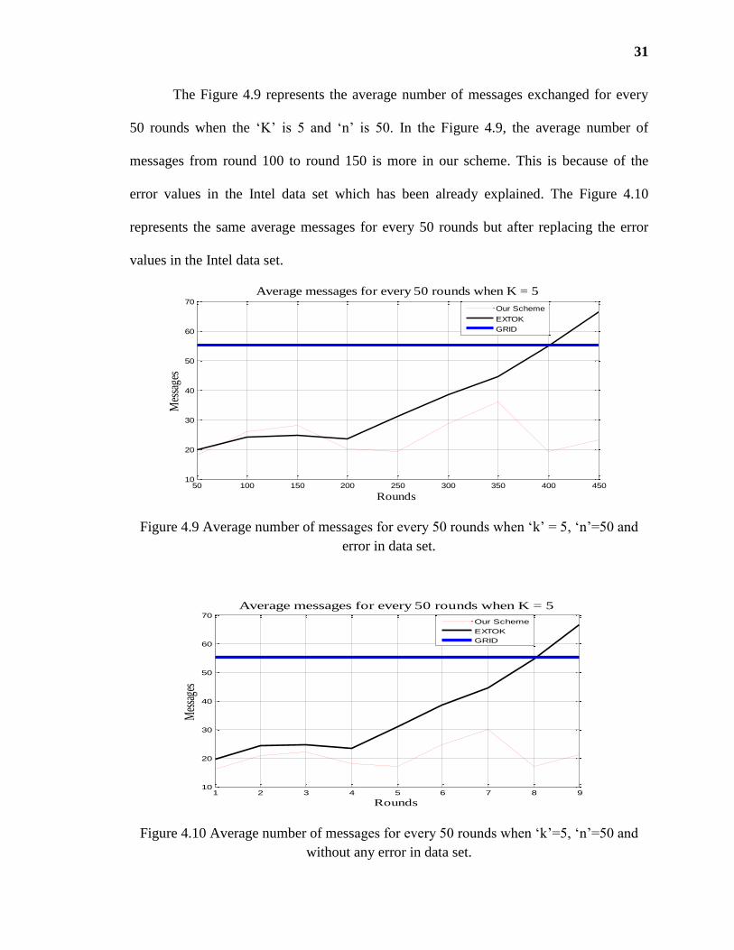
The Figure 4.9 represents the average number of messages exchanged for every
50 rounds when the ‘K’ is 5 and ‘n’ is 50. In the Figure 4.9, the average number of
messages from round 100 to round 150 is more in our scheme. This is because of the
error values in the Intel data set which has been already explained. The Figure 4.10
represents the same average messages for every 50 rounds but after replacing the error
values in the Intel data set.
Figure 4.9 Average number of messages for every 50 rounds when ‘k’ = 5, ‘n’=50 and
error in data set.
Figure 4.10 Average number of messages for every 50 rounds when ‘k’=5, ‘n’=50 and
without any error in data set.
50 100 150 200 250 300 350 400 45010
20
30
40
50
60
70
Rounds
Mes
sage
s
Average messages for every 50 rounds when K = 5
Our Scheme
EXTOK
GRID
1 2 3 4 5 6 7 8 910
20
30
40
50
60
70
Rounds
Mes
sage
s
Average messages for every 50 rounds when K = 5
Our Scheme
EXTOK
GRID

32
Our second set of experiments were performed to evaluate the performance of our
scheme with respect to different ‘k’ values. This set of experiments was also performed
to check the diversity part of our scheme. In these experiments only the ‘k’ value was
changed i.e. ‘k’ was initially 5 and then 10 and later 15. We have fixed the ‘m’ value to 4.
We have not changed the ‘m’ value as the change of ‘m’ value will not have much effect
on the energy required for communication i.e. for any given ‘m’ value the number of
messages exchanged between the nodes will be same, the changing ‘m’ value will just
have very minute impact on the processing energy, which is almost negligible. For our
experiments ‘n’ value is initialized to 30. All the experiments were performed to evaluate
Average Messages per Round, Average Energy per Round and to determine the total
number of rounds for each scheme given a constant initial energy (E=50000mJ). The
comparison of our scheme for different ‘k’ values is shown in Table 4.4.
Table 4.4 Comparison within our scheme for different ‘K’ Values
E = 50000mJ
Avg Messages/Round
Avg Energy/Round
Total Rounds for given E
OUR SCHEME
K =5 25.29 48.73 1026
K =10 23.28 47.43 1054
K =15 21.27 46.21 1082
Graphical representation of the above data can be seen in the Figure 4.11. In the
Figure 4.11, the ‘k’ values are being varied, ‘k’ = [5, 10, 15]. Each of the experiment was
done by taking an initial energy (E) of 50000mJ. Whenever the energy goes below 0, the

33
network will collapse, that means the first node in the network has died. If a node in the
network dies, the yielded results are not 100% accurate.
Figure 4.11 Comparison for different ‘k’ values within our scheme.
0 200 400 600 800 100 12000
0.5
1
1.5
2
2.5
3
3.5
4
4.5
5x 10
4
Rounds
Ene
rgy
[mJ]
For Same m, varing K values
K = 5
K = 10
K = 15

34
5. CONCLUSIONS
In this thesis, we have proposed an energy efficient scheme called Top (k,m) for
processing top-K queries with diversity m in wireless sensor network. By using the
Gaussian’s properties to estimate the probabilities of a nodes contribution to the final top-
k, we could limit the number of message exchanged between nodes and the base station.
By doing so, we have not only decreased the messages exchanged per round, but also
increased the network life time which was our primary goal. This has been
experimentally shown by comparing our results with EXTOK scheme and GRID scheme
by using different performance parameters. Thereby, we conclude that our scheme is
efficient enough for processing top-k queries in wireless sensor networks with better
network life time.
.

35
BIBLIOGRAPHY
[1] S. Madden, M.J. Franklin, J.M. Hellerstein and W. Hong, “TAG: A Tiny
Aggregation Service for Ad Hoc Sensor Networks”, Operating Systems Design and
Implementation, 2002.
[2] W. Minji, X. Jianliang, T. Xueyan, L. Wang-Chien, "Top-k Monitoring in Wireless
Sensor Networks", IEEE Trans. Knowledge and Data Engineering, vol. 19, no. 7,
pp. 962- 976, Jul. 2007.
[3] Baljeet Malhotra, Mario A. Nascimento and Ioanis Nikolaidis, “Exact Top-K
Queries in Wireless Sensor Networks”, IEEE Trans. Knowledge and Data
Engineering, vol. 23, no. 10, pp. 1513-1525, Oct. 2011.
[4] Myungho Yeo, Dongook Seong and Jaesoo Yoo, “Data-aware top-k monitoring in
wireless sensor networks”, IEEE International Conference on Radio and Wireless
Symposium, Jan. 2009.
[5] Wen-Hwa Liao and Chong-Hao Huang, “An efficient Data Storage Scheme for
Top-k Query in Wireless Sensor Networks”, IEEE International Conference on
Network Operations and Management Symposium, April 2012.
[6] Xingjie Liu, Jianliang Xu and Wang-Chien Lee, “A Cross Pruning Framework for
Top-k Data Collection in Wireless Sensor Networks”, Eleventh International
Conference on Mobile Data Management (MDM), May 2010.
[7] Hai Thanh Mai and Myoung Ho Kim, “Processing continuous top-k data collection
queries in lifetime constrained wireless sensor networks”, Fifth international
conference on Ubiquitous Information Management and Communication, Feb.
2011.
[8] Minji Wu, Jianliang Xu, Xueyan Tang, “Processing Precision-Constrained
Approximate Queries in Wireless Sensor Networks”, Seventh international
conference on Mobile Data Management, May 2006.
[9] Baichen Chen, Weifa Liang, Jeffrey Xu Yu, “Online Time Interval Top-k Queries
in Wireless Sensor Networks”, Eleventh International Conference on Mobile Data
Management (MDM), May 2010.

36
[10]
M.J. Handy, M. Haase, D. Timmermann, "Low Energy Adaptive Clustering
Hierarchy with Deterministic Cluster-Head Selection", 4th International Workshop
on Mobile and Wireless Communication Networks, 2002.
[11] Peter Bodik, Wei Hong, Carlos Guestrin, Sam Madden, Mark Paskin, Romain
Thibaux, Joe Polastre and Rob SzewczykOnline resource of Intel Berkeley lab
project, http://db.csail.mit.edu/labdata/labdata.html

37
VITA
Kiran Kumar Puram was born on 14th May 1990 in the town of Hyderabad,
Telangana, India. He received his Bachelors of Technology degree in Computer Science
and Engineering from Jawaharlal Nehru Technological University, Hyderabad,
Telangana, India in 2011. He has been a graduate student in the Computer Science
Department at Missouri University of Science and Technology since January 2012 and
worked as a Graduate Research assistant under Dr. Sanjay Kumar Madria from August
2012 to August 2014. He received his Masters in Computer Science at Missouri
University of Science and Technology in December 2014.
