to the instrument landing system yeang, chen-pang
TRANSCRIPT
ANALYSIS OF INTERMODULATION INTERFERENCE
TO THE INSTRUMENT LANDING SYSTEM
by
YEANG, CHEN-PANG
B.S., National Taiwan University, Taipei, Taiwan
June 1992
Submitted to the Department of Electrical Engineering and Computer Science
in Partial Fulfillment of the Requirements for the Degree of
MASTER OF SCIENCE
at the
MASSACHUSETTS INSTITUTE OF TECHNOLOGY
January 1996
@ Massachusetts Institute of Technology 1996
All rights reserved
Signature of Author
Department of ElectricalYngineerii (and Corri. ter Science
.January 18, 1996
Certified by
/Certified by
e (I I A ,
Accepted by..A•Ai.-USE CTS INS'I'U'TE"
OF TECHNOLOGY
APR 1 1 1996
LIBRARIES
/# Dr. Ying-Ching Eric YangThesis Supervisor
Professor Jin Au Kong
Thesis Supervisor
S-Frederic R. MorgenthlalerClhaima'an, )epar men t Conmmittee on Graduate Studeuts
.L-t-- --
`\I r-\

)

ANALYSIS OF INTERMODULATION INTERFERENCE
TO THE INSTRUMENT LANDING SYSTEM
by
Yeang, Chen-Pang
Submitted to the Department of Electrical Engineering and Computer Science
on January 18, 1996 in partial fulfillment of the requirements for the degree of
Master of Science
ABSTRACT
This thesis provides a model that could quantitatively evaluate intermodulation
interference for the localizer receivers of instrument landing system. In this model a receiver
is divided into frequency selection stage, which selects the desirable RF signal and converts
it to IF; and baseband stage, which retrieves course deviation from the localizer baseband
waveform. Both stages are characterized by a set of parameters. The parameters are
inverted by matching simulation results with experimental data for standard interference
conditions. The model is then used to predict the course deviation current under any given
interference environment.
Thesis Supervisor: Jin Au Kong
Title: Professor of Electrical Engineering
Thesis Supervisor: Ying-Ching Eric Yang
Title: Research Scientist, Research Laboratory of Electronics

-1

Contents
Acknowledgment .................................................. 7
List of Figures .......... .... ..... ........................................... 11
List of Tables ................... ....................................... ...... 13
Chapter 1 Introduction 15
1.1 Background ................................................................ 15
1.2 ILS Localizer Operating Principle .............................................. 17
1.3 Types of Radio Interference to ILS ........................................ 21
1.4 Overview of Problem and Methodology ...................................... 23
Chapter 2 Generic Model for ILS Receiver 25
2.1 Localizer Receiver Architecture ............................................... 25
2.2 Modeling of a Nonlinear Device .......................... ...... ........... 27
2.3 Modeling of Frequency Selection Stage ............. ....................... 33
2.4 Modeling of Baseband Stage ......... .................................... 44
Chapter 3 Model Synthesis 58
3. 1 Experiilllents for ILS Receiveri Inlterfeieilce(' ...................................... 58
3.2 M odel S ,tlt llesis-Inlversioll of RIeceiverI lara• I tI I('ers .......... ....... ............. .. 61
3.3 Iive I '('ive s a 1 1 reshold C rves ............................... ..... .(
Chapter 4 Simulation Results 74
4.1 Designing Future Receivers ................................................. 74
4.2 Pure-Carrier Intermodulation Interference ...................................... 78
4.3 Calculation of Course Deviation Current ....................................... 81
Chapter 5 Conclusion 83
Reference 85
Acknowledgment
I wish to express my appreciation to my advisor Professor J. A. Kong, who provides
me the chance to embark this study. His enthusiasm and kindness encourages the author
of this thesis in many aspects.
I am deeply indebted to my research mentor, Dr. Eric Y. Yang. He gave me a lot of
very precious guides and suggestions from shaping research scheme to conducting detailed
theorization and simulation as well as writing a technical text. In a sense I am enlightened
by him. I am also grateful to Dr. Robert T. Shin and Dr. A. Jordan for their direction
on me to the methodology of scientific research.
I wish to thank Mr. Yan Zhang, my research partner. Some of the important ideas
in this thesis were initiated by him. His warmth and diligence prove him a best research
partner. I also wish to thank my senior Mr. Chih-Chien Hsu. He gave me a lot of help
in familiarity with computers. My senior Shih-En Shih and my friend Tza-Jing Gung
were the ones I can always count on. I would also like to thank them for their spiritual
support. I am very fortunate to be surround with excellent persons in Professor Kong's
group, Dr. Kung-Hau Ding, Dr. Jean-Claude Souyris, Dr. Joel Johnson, Mr. Jung Yan,
other colleagues and our secretary Ms. Kit-Wali Lai.
Fi inally I wish to thank my parents for their support all these years.


" You don't want to become Buddha, nor do you want to learn alchemy "
Said the Master, " Then the only thing I can teach you is Magic "
" Gee! ", the Monkey starts to contemplate
" I heard his 108 Varieties are pretty fantastic, can I try them ? "
-- Monkey King


List of Figures
1.1 Instrument Landing System ................. ................................. 19
1.2 ILS operating principle .................................. .................... 20
2.1 ILS receiver configuration ............................................... . 26
2.2 Typical nonlinear input/output relationship .................................... 29
2.3 RF-section block diagram ......... ............. ............... 34
2.4 Block diagram of a balanced mixer ............................................. 37
2.5 Sixth-order Chebyshev filter ................................................... 40
2.6 IF-section block diagram ...................................................... 40
2.7a Configuration of AGC ................. ........................................ 43
2.7b Procedures for AGC simulation ............................................... 43
2.8a FM power spectrum. The 20-dB bandwidth is 64 KHz .......................... 47
2.81) M odeled FM power spectrum ................................................... 47
2.9 Envelope detector circuit .............................................. ...... 50
2.10 IF and baseband noise spectrum (one side) ..................................... 54
2.11 CDI output based on simulated and approximate(d clnvelopc detector ............ 57
2.12 CI)I imean and standard deviation ..................... ....................... 57
3.1 ExI)erimncental SCtup) for ILS Bl-interference tests .............................. 59
3.2 FAA intermodulation threshold test results ................................... 62
3.3 Parameter inversion procedures ................. ............................... 68
3.4 Inverted AAM RF pre-filter response .......................................... 71
3.5 Inverted ITU RF pre-filter response ............................................ 71
3.6 AAM two-frequency B1 curves ................................................. 72
3.7 AAM three-frequency B1 curves ............................................... 72
3.8 ITU two-frequency B1 curves ................. ................................. 73
3.9 ITU three-frequency B1 curves ................................................ 73
4.1 Inverted ICAO RF pre-filter response ........................................... 76
4.2 ICAO two-frequency B1 curves ............................................... 77
4.3 ICAO three-frequency B131 curves ............................................... 77
4.4 Comparison of pure-carrier interference with FM interference: AAM model ...... 79
4.5 Comparison of pure-carrier interference with FM interference: ITU model ....... 79
4.6 Comparison of pure-carrier interference with FM interference: ICAO model ..... 80
4.7 Specification of over-threshold, threshold and under-threshold conditions ........ 81
4.8 CDI distribution: over-threshold ................. .............................. 82
4.9 CDI distribution: threshold ......................................... 82
4.10 CDI distribution: under-threshold ................ ...................... 82

List of Tables
2.1 Simulated CDI for zero-noise conditions .......................... ............ 56
3.1 Intermodulation frequencies (two frequencies) ................................... 70
3.2 Intermodulation frequencies (three frequencies) ................................ 70
3.3 Inverted receiver parameters ................................................... 70
4.1 Inverted ICAO receiver parameters ............................................ 76

Chapter 1
Introduction
1.1 BACKGROUND
For the past few decades, Instrument Landing System (ILS) has been used to
provide precision landing aid for aircraft during the period of low visibility. The
operation of instrument landing system depends on the communication of radio
signals between ground-based transmitters and airborne receivers. The ILS radio
signals provide information of the aircraft course deviation, height and distance
from the landing spot. The messages retrieved from airborne sensor can be
fed into the aircraft control system. Newly developed landing systems such as
Microwave Landing System (MLS) and Global Positioning System (GPS) adopt
different spectrum regions, system architecture or coding characteristics; but they
also rely on propagation of EM waves to get information of the airplane.
- 15

Chapter 1 Introduction
Since its invention ILS has worked well for the airports around the world
without serious incidence. However, increasingly hostile radio environment around
the airports due to urban development has gradually threatened its performance.
Larger number of airport within a region makes it difficult to find ILS frequencies
for different runways without running into interfering with other radio navigation
systems. Buildings construction around the airport increases the opportunity of
multipath interference to ILS radio signals. In addition, growth of FM stations,
Industrial-Scientific-Medical equipment (ISM) and other instruments which radiate
frequencies adjacent to ILS spectrum region also aggravates interference potential.
The affore mentioned new systems is under consideration but the civil aviation
authorities also made significant effort to alleviate those existing problems. The new
landing systems utilizing different frequency band and signal processing schemes, such
as MLS and GPS, have been developed. Before the transition to new systems has
completed, however, the principal system is still ILS. Therefore the evaluation and
improvement of ILS interference immunity are very important.
An appropriate way to conduct the evaluation of automatic landing system is
to do statistical simulation on the landing process under realistic radio environment.
The statistical parameters obtained from simulation such as failure rate are the basis
for performance evaluation. In order to complete this simulation a theoretical ILS
receiver model studying at the effect of radio interference is necessary. It is known that
ILS interference comes from different types of mechanisms. In this thesis we choose
intermodulation interference to be tile target of analysis. It is because the spectrum
range of a specific ILS subsystem: localizer (108.1 MHz to 111.95 MHz) is very close
to FM broadcast band (88.1 MHz to 107.9 MHz), FM power (1 to 100 KW) is much
larger than localizer power (15W), and therefore FM broadcasting signals are capable
of driving the receiver into nonlinear region to generate interimodulation components.
The fi-eeuencies of low-order internlmodulation components, which often posses larger
power, are close to localizer band. Apparently FM interlnodlllation interferenice is a
non-negligible problem for ILS localizer.

1.2 ILS Localizer Operating Principle
The purpose of this thesis is to present an analysis of intermodulation interference
on ILS localizer receiver. A generic model based on ILS circuit configuration is
developed to cover the general population of receivers in service. This model contains
the frequency selection part which include sections from RF to IF, and baseband signal
processing part which include sections from IF envelope detector to output. The
output error as a function of interfering frequencies is simulated and compared with
empirical results. In order to invert appropriate receiver parameters an optimization
technique is adopted to fit experimental results. This generic model is then used to
extrapolate system response in other radio environments.
1.2 ILS LOCALIZER OPERATING PRINCIPLE
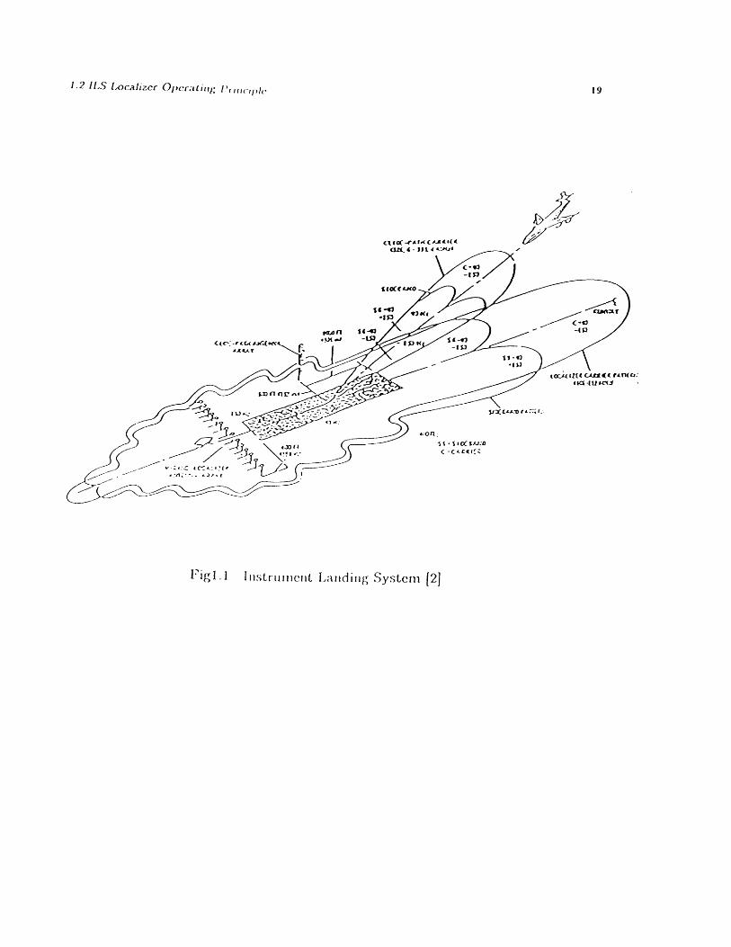
Instrument landing system (ILS) consists of three subsystems: localizer trans-
mitter for azimuth guidance, glide slope transmitter for vertical guidance and marker
beacons or distance measuring equipment (DME) for distance-to-threshold guidance.
The placement of ground systems and rough sketch of operating principles are indi-
cated in Figure 1.1. The localizer frequencies span from 108.1 to 111.95 MHz. There
are altogether 40 channels, allocated at odd 100 KHz and 50 KHz frequencies. The
glide slope frequencies span from 328.6 to 335 MHz. The DME frequencies span from
960 to 1215 MHz. These three components are tied together, so there are 40 channels
in glide slope and DME as well [10].
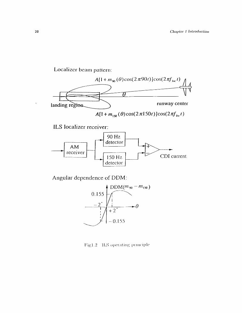
ILS localizer provides the measure of azimuth deviation of airplane from the
runway center line. Its operating principle is illustrated in Figure 1.2. The ground
system contains a set of transmitting antenna arrays near the end of runway. The
transimitted signal has two components, which are 90 IHz and 150 Hz respectively,
anmll)lit ucle-nmlodulate(d with localizer carrier frequency flo( . The arlrays are arranged
such that. the lbeamln patterns for the two Imodulated signals point to differeint sides
of the runlway and are symmmietric. Thus along the runway centerline, their signal
Chapter 1 Introduction
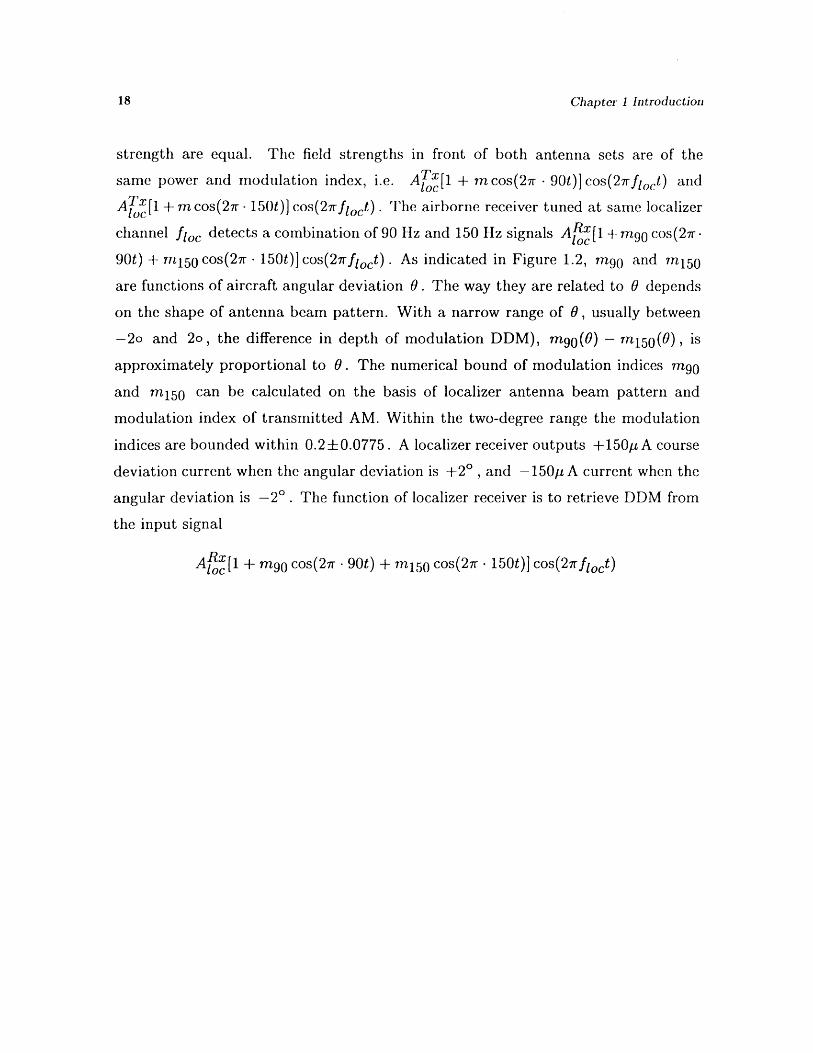
strength are equal. The field strengths in front of both antenna sets are of the
same power and modulation index, i.e. Aoc[1 + m cos(2r 90t)] cos(27rfloct) and
AT [1 + mcos(2r- 150t)] cos( 2 7rfloct). The airborne receiver tuned at same localizer
channel floc detects a combination of 90 Hz and 150 Hz signals ARx[1 + m9 0 cos(27r
90t) + m 150 cos(2r - 150t)] cos(27rfloct). As indicated in Figure 1.2, m90 and m150
are functions of aircraft angular deviation 0. The way they are related to 0 depends
on the shape of antenna beam pattern. With a narrow range of 0, usually between
-20 and 20, the difference in depth of modulation DDM), m 9g(0) - m 1 50 (0), is
approximately proportional to 0. The numerical bound of modulation indices m 90
and m150 can be calculated on the basis of localizer antenna beam pattern and
modulation index of transmitted AM. Within the two-degree range the modulation
indices are bounded within 0.2 0.0775. A localizer receiver outputs +150, A course
deviation current when the angular deviation is +20 , and -150pi A current when the
angular deviation is -2 . The function of localizer receiver is to retrieve DDM from
the input signal
AlocR[1 + m 90 cos(27r - 90t) + mn150 cos(27r - 150t)] cos(27rfloct)
al go( -eAI.( 4(AAAI(4(A-- . ... I --. ac(
S (Or(eHKO.
Ka 4 %-404%Xf "- A
-AC& CA oAA CA 7C~
(i-u -•u
VXtrAO rf g .
S- 1 I 1 SJ:O
c -CkC(ffz
Figl. Ilistrliiumint Landiing System f(2
a a
1.2 ILS Localizer Operatil, PI incilh
Chapter 1 Introduction
Localizer beam pattern.:
A + mingo (0) cos(2 r90 t) ]cos(2 7f,,t)
landing reg runway center
A [I + mso (O) cos(2 rl50t)] cos(2 xf,,.t)
ILS localizer receiver:
:urrent
Angular dependence of DDM:
0.155
-2
mr,.so )
+2
-0.155
I.i,1.2 ILS operat.ing primcip1le

1.3 Types of Radio Interference to ILS
1.3 TYPES OF RADIO INTERFERENCE TO ILS
Several physical mechanisms have been identified as possible causes of radio in-
terference to ILS. They are divided into four classes by the International Telecommu-
nication Union (ITU): Al, A2, B2 and Bi. Al is in-band interference. It refers to the
condition when the input noise spectrum directly overlaps with localizer passband
such that the amplitude of 90 Hz and 150 Hz subcarriers are changed. The band to
cause Al interference is very narrow: centered at the operating localizer frequency
it spans the width of localizer passband (several hundreds Hz). Since no other radio
communication than ILS localizer is allowed within 108.1 MHz to 111.95 MHz, the
likely source of interference is the harmonics of transmitters at other bands.
A2 covers the general adjacent-band interference. It is generated by the noise
with spectrum not exactly in but very close to localizer band such that part of it falls
in the receiver passband. The noise cannot be completely got rid of before receiver
baseband so the amplitudes of 90 Hz and 150 Hz subcarriers are changed accordingly.
A2 happens only when both localizer channel and interference spectrum are very close
to 108.1 MHz, for example, localizer channel 108.1 MHz and FM channel 107.9 MHz.
When the radio frequency is far away from the desired receiver frequency but causes
interference the mechanism is classified as B2. It occurs when the input noise power
level is relatively high. Because of the high input power the mechanism responsible
for B2 is probably receiver nonlinearity.
The type of interference dealt in this thesis is B1 - intermodulation interference.
A l, A2 and B2 can be induced by one frequency, but B2 should be induced by two or
more. Interniodulation is also the product of receiver nonlinearity. For a nonlinear
systemlll, the out)plut includes not only those frequencies which are present in input
excitation, b)ut also numiblers of harInon(ics which are the coiimbinations of the input,
fre ueilcies. Interlnodulation interference to the receiver occurs when the receiver
is d(rivell inIto a nonlinear region of operation by high-powered signal such that, the
larllonilics wilch lie within time receiver passband are geierated and appeared at the

22 Chapter 1 Introduction
output. For the intermodulation to occur, at least two signals need to be present.
And the harmonics are linear combinations of input frequencies. For example, if the
input of a nonlinear device contains two frequencies fl and f2, then the second-
order intermodulation components occur at fl + f2 and fl - f2, the third-order
intermodulation components occur at 2 fl + f2, 2 fl - f2, 2f2 + fl and 2f2 - fl ,
and so on. Even if all the interfering frequencies lie out of the receiver passband, their
intermodulation components can fall right at the desired frequency. The proximity of
FM broadcasting frequencies to ILS localizer band makes localizer receiver susceptible
to FM-generated intermodulation interference.

1.4 Overview of Problem and Methodology
1.4 OVERVIEW OF PROBLEM AND METHODOLOGY
The calculation of intermodulation products from multiple input frequencies has
been known to be a tedious problem [11] [28]. In the past half century intensive study
of intermodulation interference in communication and broadcasting technology have
been conducted. Some of the most distinguishable cases of interest can be found in
wireless communication circuits [6] [8] [13] [14] [22] and cable TV circuits [1] [4] [18]
[22]. Most literature put emphasis on analyzing intermodulation effect of individual
nonlinear device, for example, RF amplifiers and mixers. However, quantitative study
of intermodulation on the whole system has been lacking. The latter is important for
analyzing the interaction between RF systems and control systems, as in the case of
ILS-driven aircraft automatic landing system. Only when we construct the model of
whole system on the basis of available empirical data can we achieve this goal.
Out of this concern, the aviation community has studied ILS interference problem
through a series of bench experiments on different kinds of operational receivers.
These experiments consist of measuring the "threshold" of interfering power as a
function of frequency under Al, A2/B2 and B1 conditions. Regression formula
derived from the performance of typical receivers were derived. These empirical
formula is important for radio environment evaluation since they specify the cut-off
level at which interfering power is considered intolerable.
However, the regression curves specify the threshold conditions only. They do
not provide the information of ILS response to the cases under or above the threshold
conditions. Thlis information is important for the overall simulation of aircraft landing
process. Therefore a receiver simulation model is necessary. Since it is impossible to
run tihe detailed simulation for all kinds of ILS receivers on the miarket, we develotp a
"gelieric" M11odel based o011 tihe regressioll formula. The ilmethodology is described
as follows: (1) Based oil real operations of ILS receivers and certain accept able
assulmill)tiolls, a simplified llatlienmatical nmodel is derived. This niodel is characterized
b)y a set, of parammeters. (2) Thie paramneter values are inverted(l fronil a set of regressionl

Chapter 1 Introduction
curves. In this thesis two-frequency B1 curves are chosen as the objective to be fitted.
(3) Apply the model to other conditions and compare the simulation results with new
regression curves to verify the consistency of the generic receiver model.
The following chapters are arranged as follows: Chapter two is the detailed
description of mathematical model. It includes frequency selection stage which
converts RF into IF signal and baseband stage which extracts course deviation
current from IF signal. Chapter three is the synthesis of receiver model with
respect to empirical results. It contains the experimental procedures for ILS B1 test,
regression formula for experimental results, inversion procedures for retrieving values
of parameters, the values of receiver parameters inverted from regression formula of
two-frequency intermodulation, and simulated threshold curves. Chapter four extends
current model to different interference conditions. It includes the extrapolation of
future-standard ILS receivers, simulation on pure-carrier intermodulation interference
and CDI calculation under non-threshold interference conditions.

2.1 Localizer Receiver Architecture
Chapter 2
Generic Model for ILS Receiver
2.1 LOCALIZER RECEIVER ARCHITECTURE
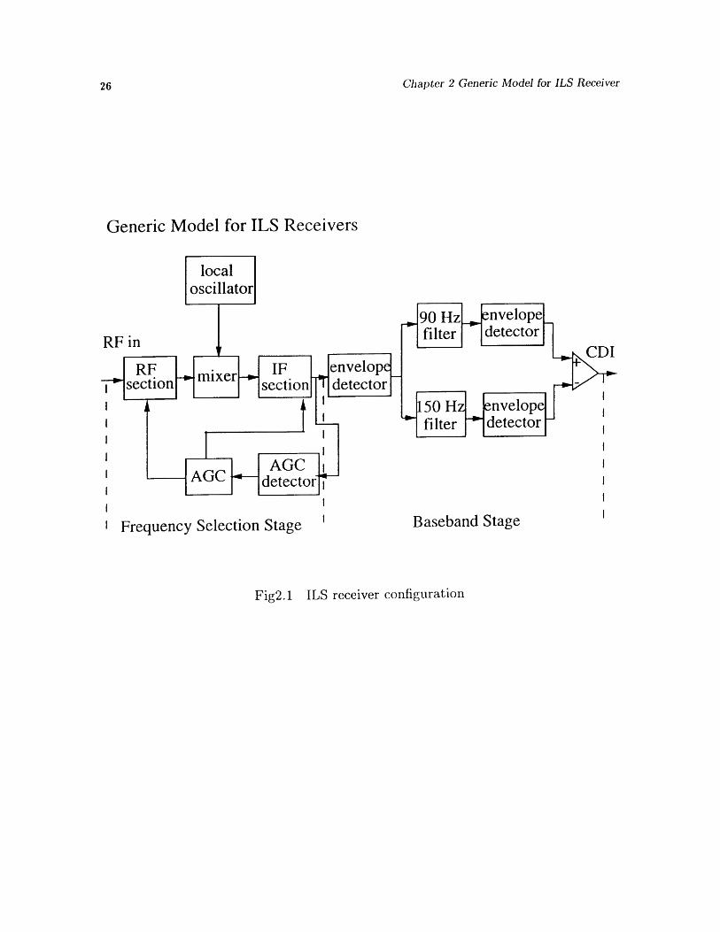
The configuration of localizer receiver is in Figure 2.1. There are two principalstages in the receiver. The first stage, or frequency selection stage, recovers basebandsignal from its amplitude-modulated form. It functions like a regular AM receiver,converting RF input into baseband output. At the very front an RF section filters
and amplifies the input. Its output is fed into a mixer which multiplies the incoming
RF signal by a local oscillator carrier to down-convert the operating frequency to IF.The IF signal is filtered and amplified in IF section. After IF an envelope detectoris followed to detect the amplitude of IF output. Baseband signal is retrieved at theoutput of envelope detector. In additional to RF, mixer and IF, Automatic GainControl (AGC) which confines the output power level of frequency selection stagewithin a narrow range is also incorporated.
Chapter 2 Generic Model for ILS Receiver
Generic Model for ILS Receivers
RF inCDI
Frequency Selection Stage I Baseband Stage
Fig2.1 ILS receiver configuration

2.2 Modeling of a Nonlinear Device
The second stage converts processed IF signal into Course Deviation Indicator
(CDI) current. We shall call it baseband stage. Baseband signal is splitted into
two paths: the first one contains a 90 Hz-centered bandpass filter and an envelope
detector, the second one contains an 150 HZ-centered bandpass filter and an envelope
detector. The output of the two paths are fed into a differential amplifier to get the
course deviation current. Among all the sections IF envelope detector is the interface
between the frequency selection stage and the baseband stage. In the following
paragraphs IF envelope detector is attributed as a part of baseband stage.
A generic receiver model is built by linking all the models of function blocks
in Figure 2.1 and cascading them together. The following sections will discuss the
construction of frequency-selection-stage model and baseband-stage model in more
detail. The modeling of a single nonlinear device is necessary before starting a
macroscopic consideration.
2.2 MODELING OF A NONLINEAR DEVICE
Intermodulation interference is the result of receiver nonlinearity. For modeling
purpose, we consider a nonlinear system S with one input x(t) and one output
y(t). Similar to the way a linear system is represented by an impulse response
h(t), a nonlinear system will be represented by a series of impulse responses hl (t),
hI2 (tl, t2 ), h 3 (t 1 t2, t3), .... such that
(t)= / dT1 ... dThi(T1,...,rj)x(t - T1 ) .. x(t - i) (2.2.1)

Chapter 2 Generic Model for ILS Receiver
The form of (2.2.1) is called the Volterra-series representation [27] [29]. This
representation takes into account not only high-order terms due to nonlinearity but
also the temporal variation. In general y(t) cannot be expanded into a power series
of x(t) but is a integral-transform type series with which transfer functions hl(t),
112(tl, t2 ), .... are involved.
Rather than sticking to this rigorous but complicated proposition, the thesis
assumed that output y(t) is a functional of input x(t).
y(t) = F(x(t)) (2.2.2)
This assumption is correct if the operating amplitude and frequency are within
reasonable regions. For example, to the first-order approximation the capacitive
effect of a PN junction could be ignored and diode current (output) Id(t) is related
to diode voltage Vd(t) by the formula Id(t) = Io(exp(Vd(t)/VT) - 1). The source of
ILS receiver nonlinearity is mainly amplifier. It is well known that temporal variation
is secondary in nonlinear amplifiers like FET or BJT. Modeling i/o relationship as a
functional is a valid approximation. If y is a function of x then it could be expanded
into a power series of x:
y = Kxz (2.2.3)i=1
How many terms should we keep in order to cover the dominant nonlinear effect
depends on the function itself and input amplitude. For a nonlinear amplifier, the
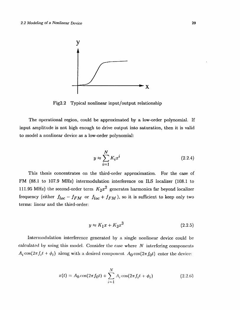
in)put/output relationship usually resembles a curve like the one in Figure 2.2.
2.2 Modeling of a Nonlinear Device
y
Fig2.2 Typical nonlinear input/output relationship
The operational region, could be approximated by a low-order polynomial. If
input amplitude is not high enough to drive output into saturation, then it is valid
to model a nonlinear device as a low-order polynomial:
N
yx Ki x i (2.2.4)i=l
This thesis concentrates on the third-order approximation. For the case of
FM (88.1 to 107.9 MHz) intermodulation interference on ILS localizer (108.1 to
111.95 MHz) the second-order term K 2 x 2 generates harmonics far beyond localizer
frequency (either floc - fFM or floc + fFM ), so it is sufficient to keep only two
terms: linear and the third-order:
y K1 x +1 +- K 3 x3 (2.2.5)
Intermodulation interference generated by a single nonlinear device could be
calculated bly using this model. Consider the case where N interfering components
Ai cos(27rft -4- 0i) along with a desired component Ao0 os(27rf 0 t) enter the device:
Nx(t) = A0 cos(2 7rf 0 t) + t Ai cos(2T fit + 4i) (2.2.6)
i==1
Chapter 2 Generic Model for ILS Receiver
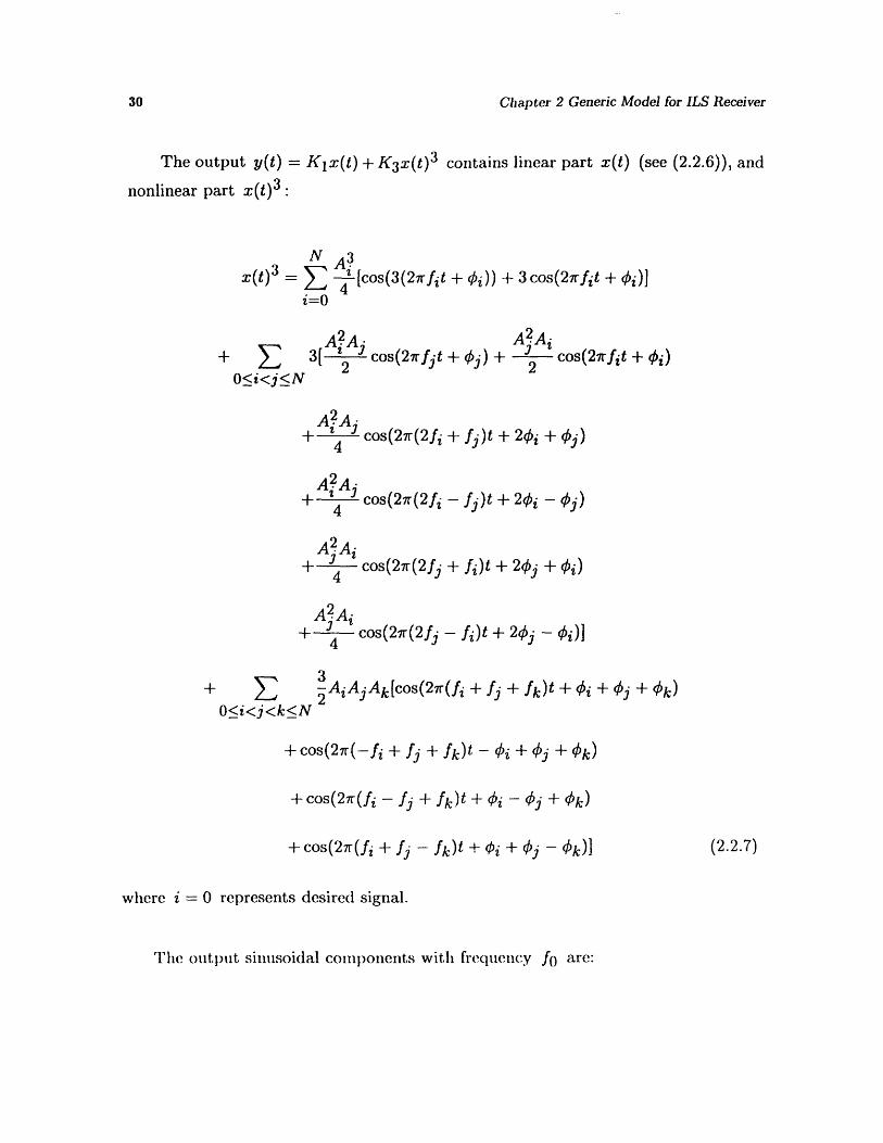
The output y(t) = Kjx(t) + K 3 x(t) 3 contains linear part x(t) (see (2.2.6)), and
nonlinear part x(t)3 :
N A3=(t)3 - [cos(3(2wrfit
i=O
A2 A+ 3[ 2 cos(27rfjt
O<i<j<N
A2 A+ 4 cos(27r(2fi
+ cos(2~(2fi
A2 A-+ 4 cos(27r(2fj
+ 0i)) + 3 cos(27rfit + 0i)]
A2 Ai+ j) + 2 cos(21rfit +
+ fj)t + 20i + 0j)
- fj)t + 20i - j)
+ fi)t + 20j + 0i)
A2Ai+ • cos(2r(2fj - fi)t + 20j - i)]
4
+ OjO<i<j<k<N
2AiAjAk[cos(2r(fi + fj + fk)t + Pi
+ cos(27r(-fi + fj + fk)t - €i + ±j + €k)
+ cos(27(fi - fj + fk)t + 0i - ±j + Ok)
+ cos(27r(fi + fj - fk)t + ¢i + Oj - k)0]
where i = 0 represents desired signal.
The output sinusoidal components with frequency fJ are:
+ Oj + ¢k)
(2.2.7)

2.2 Modeling of a Nonlinear Device
(a) K 1Ao cos(2rf0ot)
(b) 4K 3 A 03 cos(27rf 0 t)
(c) EN_1 3K3 AoA cos(27rf 0t)
(d) 2f-fj=fo •A Ajcos(27r(2fi - fi)t + 20i - j)
(e) Efi+fj-fk=f AiAjAk cos(2r(fi + fj - fk)t + €i + j - 46k)
(a) is the linear term. (b) is generated by third-order intermodulation of localizer
frequency with itself, fo - f0 + f . It is named 'self-modulation' component [23]. (c)
is generated by third-order intermodulation of localizer frequency with one interfering
frequency, fi-fi+fo. It is named 'cross-modulation' components [22]. (d) and (e) are
generated by third-order intermodulation of two and three interfering frequencies. (b)
and (c) have exactly the same spectra as localizer signal (a) since no qi(t) appears in
the phases. They essentially modifies the amplitude of localizer signal but eventually
would not effect the output CDI value. So (b) and (c) can be seen as parts of signal.
Combination of (d) and (e) is third-order intermodulation interference generated by
device nonlinearity. To summarize, the signal part at output is
[KIA + + K3A0 3 A0 A 2]cos(27rfot)i=1
And the interference part is
3 K 3 A Aj cos(27rf 0 t + 25i - j)+2ffi-j =ffo
2 I3AAAk cos(27rfot + 5i + cj - Ok)fi+fj--fk-=fo

Chapter 2 Generic Model for ILS Receiver
Let the summation of these two parts equal to y(t). Its total amplitude depends
on phases 41, 2,.... In the case of ILS localizer, the most serious source of
intermodulation interference is FM broadcasting. The phases of FM carriers are the
messages to be transmitted, therefore they are functions of time. In general they are
stochastic processes and uncorrelated with one another. The ensemble average power
of y(t) is the summation of coherent (signal) power and incoherent (interference)
power:
3N 22 < y(t) 2 >= [K 1AO + 4K3Ao3 + j -K 3 AoA?]
i=1
+ 29 2•A + 9K2A2A2 (2.2.8)163 4 3 i j k(2.2
2fi-f=fo fi+fj-fk fo
Taking the square root of average power to be the effective amplitude, the fo
component at the output becomes
y(t) < y(t) 2 > cos(27rfot + q) (2.2.9)
Equation (2.2.8) and (2.2.9) apply to other frequencies as well. They provide the
formulation to calculate a nonlinear device's output.
2.3 Modeling of Frequency Selection Stage
2.3 MODELING OF FREQUENCY SELECTION STAGE
In a receiver the RF signal should be processed and converted into baseband
signal. This is done by frequency selection stage. As indicated in Figure 2.1, the
frequency selection stage consists of RF, mixer, and IF sections, like a typical AM
receiver. A realistic AM receiver may have more than one IF section. In our simplified
model only one IF section is presented. This should not, however, affect the simulation
results significantly.
In the frequency selection stage model we also only need to treat either localizer
signal or undesired FM interference at a specific broadcasting frequency like a pure
carrier, and leave those detailed phase terms to the baseband signal processing stage.
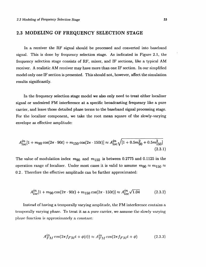
For the localizer component, we take the root mean square of the slowly-varying
envelope as effective amplitude:
A"n[1 + mgg cos(27r 90t) + m1 5 0 cos(27r 150t)] . A [1 + O.5m 0 + 0.5m250
(2.3.1)
The value of modulation index m9 0 and m 1 50 is between 0.2775 and 0.1125 in the
operation range of localizer. Under most cases it is valid to assume m 90 1 1.m1 50
0.2. Therefore the effective amplitude can be further approximated:
Aloc[1 + m90 cos(2r - 90t) + m150 cos(27r - 150t)] A AlocV/i.0i (2.3.2)
Instead of having a temporally varying amplitude, the FM interference contains a
tellmporally varying phase. To treat it as a pure carrier, we assume the slowly varying
phase flinc:tion is approximately a constant:
Az7.1 cosI( (2 rfFAt )) cos(2 r fF + 0 )) (2 )(2.3.3)

Chapter 2 Generic Model for ILS Receiver
The pure-carrier approximation is valid since either the localizer signal bandwidth
(no more than several KHz) or the FM bandwidth (64 KHz for standard test
condition, see [20]) is much narrower than RF (88 to 112 MHz), RF bandwidth
(several MHz) and IF center frequency (5 to 30 MHz).
2.3.1 RF Section
Xin Xout
Fig2.3 RF-section block diagram
Figure 2.3 is a RF-section block diagram. It contains an RF pre-filter, an
amplifier and a post-filter. A pre-filter is often a tuned LC circuit or other equivalent
passive bandpass filter. It can be characterized by a frequency response function
H"F(f) = Hr (f)I exp(i RreF(f)) For an input x(t) = N1 A i cos(27rfit+ i), the
output of pre-filter is y(t) = E 1 Hp Fi)ji cos(2rfit+ 4 ()) Typically
IHRrF(f)I peaks around the center frequency fc and drops monotonically on both
sides. The center frequency fc is usually tunable with localizer frequency floc. The
filter transfer function is usually normalized such that the peak value is unity. Here we
adopt the same convention to split RF pre-filter characteristics into two parameters:
normalized filter response and front-end gain:
lHRFold(f) HI. (f) (2.3.4)
where JIHF (fc) = 1.
The RF post-filter is modeled exactly the same way as pre-filter excCp)t with a
(different frequency response Hp (f) and normalization constant AI "

2.3 Modeling of Frequency Selection Stage
The RF amplifier is often a transistor device such as field effect transistor (FET).
The effect of temporal variation in this kind of device is considered secondary within
the operating frequency range. However its nonlinear effect cannot be ignored. The
model described in Section 2.2 could apply here. From experiments it is observed
that nonlinearity of RF amplifier K3 /K 1 varies with different input power levels [7].
In this thesis, third-order nonlinearity is specified at few discrete input power levels.
Given Hprelf\ Apre KK post post
Given HrF( f) , A RF K3 , K1, HRF (f , RF and input amplitude for
each frequency component, the amplitude of each frequency at RF output could be
evaluated. Ideally a pre-filter is very selective so that all interference other than
localizer frequency is suppressed. But it is difficult to implement such a filter.
Separation between localizer and FM is less than 200 KHz, a bandwidth RF filters
could hardly achieve. Thus significant amount of energy in the FM signal can pass
the filter and cause intermodulation interference. The interference amplitude is a
function of pre-filter response at input FM frequencies Hre(f1 ), H•' .e2 ). .If
RF pre-filter and post-filter cannot suppress interference well, then nonlinearity after
RF section has to be considered. In this case mixer would produce non-negligible
intermodulation interference.

Chapter 2 Generic Model for ILS Receiver
2.3.2 Mixer
Mixer is also a nonlinear device. Unlike an amplifier, a mixer has two input:
one is from RF section and the other is from local oscillator. Ideally the output of a
mixer is the product of two inputs. Without interference, the RF-section output is
pure localizer signal x(t) = AOR F cos(21rfloct) . The local oscillator output is a pure
sinusoidal wave xosc(t) = Aosc cos(2irfosct + Oosc) , where the frequency difference
between both is IF, Ifosc - flocl = fIF - fosc could be larger or smaller than floc.
In the model we assume a superheterodyne receiver, i.e. fosc - floc = !IF . Thus
the ideal mixer output y(t) is
y(t) = x(t) -. osc(t) = AORFAosc/2[cos(21r(fosc + floc)t + 0osc)
+ cos(27r(fosc - floc)t + qosc)] (2.3.5)
The first term, which is far above the IF band, can be removed by the IF filter.
A real mixer contains more terms than (2.3.5). We consider the following
approximation model represented by the fourth-order Taylor series expansion over
two variables: Generally a mixer is a nonlinear 'three-port'. The output y is a
function of x and Xosc. It can be expanded into a Tayler series
y = f(z, Xosc) = f(xo, xzosc) + o( )o+ sc )oX0
( 2 + 2 ( xxo + (o 2 f f:2o+ ++s +z os
ta3 f af 03f ( j3 . 3K XXsc +)
o 0 o (oS) 0)
S( f x4 0f "3 1 9 2 2+4( +4 x + o6 , x, .... OSC

2.3 Modeling of Frequency Selection Stage
+4 04jf XX +o3sc t- ox sc + H.O.T. (2.3.6)
where O represents operating point, e.g. () ° means the value of function (_-)at the operating point (x, Xosc) = (x0 , Isc) . H.O.T. refers to high-order terms.
It is obvious that in (2.3.6) the odd-order terms do not lie in the IF passband
provided input frequencies are not far from RF. Unlike a nonlinear amplifier, the
relevant intermodulation components of a mixer are second-order, fourth-order,...
and so on. XXosc provides desired localizer signal, x2 and x2sc generate baseband
frequencies and fourth order plays the role of amplifier's third order. For example, if
there are two interfering frequencies fi f2 satisfying 2fl - f2 = floc, then X3 Xosc
would produce intermodulation term with frequency fosc - fl - fi + f2 which is
exactly equal to fIF (fosc - floc)"
Eight terms in (2.3.6) should be kept (second and fourth order) to include both
linear and third-order intermodulation effects. This means generally a mixer is
characterized by eight coefficients, which makes the model more complicated. We
shall consider a simpler but realistic situation, i.e. the balanced mixer. The balanced
mixer uses two symmetric nonlinear devices to eliminate the first-order components.
Its configuration is in Figure 2.4.
-1
XXOSC )
out
XOSC )
Fig2.4 Block diagraml of a balanced inixer

Chapter 2 Generic Model for ILS Receiver
The output of a balanced mixer y(t) is a nonlinear function of x and Xosc with
form:
y = g(x + Xosc) - g(x - Xosc) = g(1)(o) • 2xosc + g(2 )(o) -2xxosc
+1/3g(3 )(o) - (3x 2Xosc + Z3sc) + 1/3g(4)(o) (x 3Xosc + X3scx) + H.O.T. (2.3.7)
Among the lower-order terms in (2.3.7) the ones capable of generating IF are
g(2 )(o) 2zxosc and 1/3g(4 )(o). (x 3 Xosc+ X3scz). Let 2g(2 )(o) = K 2 , 1/3g(4 )(o)=
K 4 , x = N= An cos(2rfnt + On) and Xosc = Aosc cos(2irfosct + osc) . Substitute
into (2.3.7) and get rid of out-of-IF-band components, the resultant y would be
N
y = (1/2K 2 Aosc + 3/8K4 Aosc3 ) E An cos(27r(fosc - fn)t + qosc - On)+n=1
M1/2K 4 A o sc E Bm cos(27r(fosc - fm)t + Oosc - Om) (2.3.8)
m=1
where Em=1 Bm cos(2r fmt + Om) = N An cos(27rfnt + On) 3
Therefore the operation of balanced mixer resembles that of a nonlinear amplifier
with linear coefficient 1/2K 2 A os c +3/8K4 Aosc 3 and third-order nonlinear coefficient
1/2K 4 Aosc, except that every sinusoid contains a phase difference qosc. Only two
coefficients are required to characterize a balanced mixer.

2.3 Modeling of Frequency Selection Stage
2.3.3 IF Section
Generally IF section is similar to RF section, but they differ from each other in
several aspects. The IF filter is much more selective than the RF filter. In the case
of ILS localizer the 3-dB bandwidth is usually no more than 100 KHz, and at least
60 to 80 dB attenuation would be reached for the FM interference. The IF amplifier
can also achieve higher gain than is possible for RF amplifier. A common IF circuit
consists of a highly selective crystal filter followed by a series of cascading amplifiers.
The crystal filter corresponds to IF pre-filter. Typically IF filters used in localizer
receivers are implemented as Chebyshev filters having order 6, 8 or 10 [26]. For the
worst-case consideration, sixth-order Chebyshev filter is used in receiver model. It
has the magnitude response:
1H e (2.3.9)f1 + 1.512T12(f)
where T1 (f) = 4TO3(f) - 3TO(f), To(f) = B f 2)
The frequency response of sixth-order Chebyshev filter is demonstrated in Figure
2.5.
The amplifier set is not only a nonlinear device but also contains RC circuits
that serve as filters. It corresponds to IF amplifier and IF post-filter. Notice that IF
amplifier may perform a better linearity either because more linear device could be
used (e.g. BJT) or more delicate design could be applied to reduce nolincarity (e.g.
log amplifier) under lower frequency range. Because IF pre-filter is highly selective,
illtermnodulatioIL at tie IF amlplifier is negligible unless incoming FM interference
is extremlnely large. In our receiver imodel IF section is characterized by a sixth-
order Clmlebyslhev p)re-filter Hl) ,' a 'good' amplifier withl large linear gain K[IF andIF
Ilegligible noilimar coefficient K IF , an11 a fiat, post-filt'er Httl . Figure 2.6 is IF-
s -ech(.iin block (liagraImI.

Chapter 2 Generic Model for ILS Receiver
Chebyshev Filter (Center= 30.5MHz, BW=50kHz)
0
-10
-20
-30
-40
-50
-60
-70
-Rn
-400-300-200-100 100 200 300 400
frequency deviation from center (kHz)
Fig2.5 Sixth-order Chebyshev filter
Xout
Fig2.6 IF-section block diagram
X

2.3 Modeling of Frequency Selection Stage
2.3.4 Automatic Gain Control
Automatic Gain Control (AGC) is the mechanism that keeps output voltage
approximately at a constant level. AGC is a simple feedback control system. Its
structure is indicated in Figure 2.7a. An AGC detector at the IF output is responsible
for the detection of output voltage level. Sometimes it is just the IF envelope detector.
When the input level increases too much such that output level exceeds the allowable
range, the detected level from AGC detector drives AGC control circuit to decrease
the RF as well as IF amplifier gain. Therefore output voltage level comes back within
range. The reverse operation is carried out when input level is too low. For an ILS
localizer receiver AGC is necessary to implement in frequency selection stage in order
to fix the voltage level at the output of IF envelope detector (see Figure 2.1).
In practical term, we need to consider several points to implement the AGC
simulation model. First, the term "voltage level" is ambiguous. What is the exact
quantity to trigger AGC operation? The purpose of AGC is to confine the envelope
level of IF output so that the output of AM detector (i.e. the input of baseband
stage) is roughly a constant. With respect to this consideration the time average of
envelope-detected output is a good measurable. But to obtain this quantity one would
need the knowledge of individual phase terms. To avoid the complication in involving
the phase we use another quantity as the AGC input: the square root of the sum of
the amplitudes at all frequency components. For an IF output j:i Ai cos(27rfit + i) ,
the average amplitude level Eil 2A should lie within the designated range, or else
AGC is triggered to pull it back.
Chapter 2 Generic Model for ILS Receiver
The exact mathematical relationship between IF average amplitude level and
linear/nonlinear coefficients of RF/IF amplifier is determined by circuit analysis, and
varies with different kinds of receivers. For a generic receiver model the following
iterative algorithm is a reasonable approximation: if the output level is beyond upper
(or lower) limit of the designated range, then K1KR, K , K I F , and K I F are
decreased (or increased) in small steps. The same input is applied and the same
process is repeated again until the output level falls into the specified range. This
mechanism is indicated in Figure 2.7b. The underlying assumption of this model is
that RF/IF nonlinearity K 3 /K 1 keeps exactly the same no matter how large the
automatic gain control signal is fed into the amplifier. However it is not always true.
Take an FET amplifier as an example. The gain of an FET amplifier is controlled
by gate voltage. When different gate voltage values are applied, the amplifier has
different i/o curves. These curves could have different nonlinearity K 3 /K 1 near
the operating point. This problem becomes worse when input level is so large that
amplifier is saturated, which means the polynomial model is no more appropriate for
the amplifier. If input localizer and interference power is small enough such that the
amplifiers are still 'weakly nonlinear', then the above assumption is valid.
Therefore AGC could be simulated in the following procedures.
(1) Pick up initial values for KRF, KRF, KIF, KIF
(2) Run the frequency-selection stage simulation
(3) If the summation of every sinusoidal component's mean power at IF output is
above/below the prescribed range, then decrease/increase KRF, KRF , KIF, KIF
by the same ratio. Go to (2).

2.3 Modeling of Frequency Selection Stage
Fig2.7a Configuration of AGC
xili
Root-mean-square detection:N
xout(t)= - An cos(2frft + m,, )7m=1
NV0 = I At 2
I--I
Fig2.71)b ProccduIes for AGC sinulat ion
outputxout (t)

Chapter 2 Generic Model for ILS Receiver
2.4 MODELING OF BASEBAND STAGE
The localizer signal at IF output
AlocF [ + m 90 cos(27r - 90t) + m 150 cos(27r - 150t)] cos(27rflFt)
is converted into CDI output Abase (i - mi15 ) via the baseband stage. As
indicated in Figure 2.1, the IF signal is processed by an envelope detector first.
The amplitudes of 90 Hz and 150 Hz components are retrieved by a 90 Hz and a
150 Hz detector and are passed through a comparator to get the CDI output. Unlike
frequency selection stage, the baseband stage model is a statistical model because the
interference signal is random in nature. We should apply the Monte Carlo technique.
The objective of this section is to construct a simple relation of CDI with IF interfering
power, given modulation depth mgg0 and m150 .
2.4.1 Conversion of Frequency Selection Output Into Baseband Input
There is an essential distinction between the frequency selection stage model and
baseband stage model. Frequency selection stage model treats either localizer signal
or undesired FM interference at a specific broadcasting channel as a pure carrier. Its
task is to evaluate the frequency and amplitude of each carrier at IF output. So the
IF output xIF calculated by model can be represented as follows:out
NIF F IFcos(2,rI IF Vout= AO cos(2 flFt)+ cos( flFt f ) + Ai cos(27rfit+ki) (2.4.1)
i=1
where AIf' cos(27rflFt) is the intermodulation interference with frequency exactly
at localizer IF.
2.4 Modeling of Baseband Stage
On the other hand, baseband stage should take the temporal variation of localizer
amplitude and FM phase, which were hidden in frequency selection stage model, into
account since its objective is to detect out the very low frequency components. So
the detector input xdet should be
xdet = AIF[l + m90 cos(2r - 90t) + m150 cos(27r - 150t)] cos( 2 7rflFt)+
NAIF oIFst27 V'lt 2Aintf cos(2rfFt (t)) + Am cos(2rfmt + m(t)) (2.4.2)
m=1
Frequency selection stage model only provides each component's amplitude value
( AF, Anf' or Ai) and frequency value (fIF or fi). It doesn't provide the
information of modulation indices m9 0 and m 150 and phase functions IF(t)
and Oi(t). Modulation indices are inherent in localizer input. They are set at the
beginning. Phase functions are important parts of the FM signal. The baseband
stage model should include their effect. The phase function of an FM input channel
is time integration of audio message. It may also involve more signal processing like
stereo and pre-emphasis in frequency domain in order to improve the performance
[20]. In the model we convert the effect of phase functions on baseband stage to
the effect of spectra. Each RF input component is not treated as a carrier with
varying phase in time domain, but a collection of multiple frequencies with a specific
spectrum, so does the IF output components in (2.4.2). Take for example the third-
order intermodulation product fl + f2 - f3. Suppose at IF output the amplitude
of this component (as evaluated by frequency selection stage model) is A, then its
spectrum is approximately the convolution of three FM channels fl, f2 and f3, with
center frequency Ifl + f2 - f3 - foscl , and total power 0.5A 2 . (Strictly speaking, the
resultantt spectrum is derived from (1) the convolution of fl , f2 and f 3 channels after
RF pre-filter, and (2) the convoltution of IF iml)ulsC response with (1). The spectra
after RF filter are slightly differcnt, from those of FM input spectra. And the l)rod((ct's
sl)ectrullll after IF is slightly (lifferent from that, at RF section.) Mathemnat.ically,
the colnversion of p)hase-fllnctio• effect in (2.4.2) into contitnuous spectrul is tHt,
i1p)leineint.attion of F(ourier transform:

Chapter 2 Generic Model for ILS Receiver
+ooA i cos(27rfmlt + Pm(t)) = J dfHm(f) exp(i • 2rft) (2.4.3)-- OO
Under intermodulation condition, the dominant interference term is the one
with carrier frequency exactly the same as localizer signal, i.e. Aint cos( 2 rfIFt +
int~f(t)) in (2.4.2). The other interfering components are suppressed to a large
extent by IF filter. Even though some are passed, they usually fail to penetrate
the extremely sharp baseband filters. Therefore this kind of noise could desensitize
CDI output value via automatic gain control, but has no direct contribution to
'in-band' interference. The only spectrum we need to model at IF output is that
of Ant cos( 2 fnFt ff(t)) Notice that the FM noise can not be seen as
deterministic. It is a stochastic process, so is its spectrum.
2.4.2 The Construction of Baseband Stage Model
Several observations are essential for the construction of an accurate and simple
baseband stage model.
(1) It has been shown in Section 2.4.1 that in baseband stage input (2.4.2) only three
variables are relevant: localizer amplitude AIF IM interfering amplitude AIFSloc intf
and spectrum of IM interference. Given these three variables the CDI value could be
calculated.

*R8 3.86 kIHz 8 3.88 kHz ST 333.1 aecC
Fig2.8a FM power spectrum [20). The 20-dB bandwidth.is 64 KHz.
< INFM (f 2 >
fIi, -' j
IFig2.81t Modlled(i FIN1 po)()wr s')('ct, rI1iII
2.4 Modeling of Baseband Stage
-- J FM 0 JFM
f

Chapter 2 Generic Model for ILS Receiver
(2) Due to Automatic Gain Control the sum of localizer power and total interfering
power 1.04AIF 2 + AIF 2 i= A is approximately constant. Therefore theloc inf Z z
variable localizer amplitude AIF can be replaced by the square root of total
interfering power Pintf n= AFf + Z1 Ai.
(3) Monte Carlo simulation is carried out for CDI evaluation. Since FM signal is
a stochastic process, the spectrum mentioned here refers to the ensemble average
of the Fourier transform of waveform in time domain, i.e. average spectrum. The
IM spectrum in real radio environment differs from that in experimental condition.
In real environment IM interference is the product of three FM signals, therefore
the shape of its spectrum is the convolution of three FM spectra. In B1 immunity
experiments one FM channels along with two pure carriers are served as input noises,
so the shape of IM spectrum is the same as FM spectrum. Because the reproduction
of experimental results is the pre-requisite to the theoretical works proposed here,
the latter condition is adapted in our model. International Telecommunication Union
(ITU) has defined the average power spectrum of an FM channel used in interference
immunity experiments on ILS localizer receivers [20](see Figure 2.8a). The FM
spectrum in Figure 2.8a has the 20-dB bandwidth 34 KHz. The power of frequency
components outside the bandwidth is at most 0.01 times of that at center frequency.
For simplicity we could assume that their contribution is negligible. In this thesis
the shape of ITU FM power spectrum SFM(f) is approximated as a triangle within
bandwidth BW and vanishes out of bandwidth, as in Figure 2.8b. The absolute
value of average FM spectrum HFM(f) equals to V/SFM(f). Based on average FM
power spectrum Monte Carlo simulation on baseband model is possible. The ensemble
average and standard deviation of CDI values are functions of total interfering power
and IM interfering power.
2.4 Modeling of Baseband Stage
(4) Baseband stage model should confirm to the ILS localizer receiver standards when
there is no interference. First, CDI current is proportional to DDM (= m90 - m15 0 ).
If DDM= d corresponds to CDI= cIL A, then DDM= -d corresponds to CDI= -cpL A.
Second, at full deflection DDM=0.155 corresponds to CDI current 150/LA. Before
feeding into noise baseband stage model should be calibrated accordingly.
We use the following procedure to estimate CDI mean and standard deviation:
1. Calibrate the parameters of baseband stage model under signal-only conditions.
The conditions needed to be satisfied are that (1) the simulated CDI equal to 150
p•A when DDM=0.155; (2) if the simulated CDI value is cI A when DDM value is
d, then the simulated CDI value will be -cIp A when DDM value becomes -d. 90
Hz filter gain and bandwidth, 150 Hz filter gain and bandwidth, and comparator gain
are adjusted accordingly.
2. Choose the appropriate DDM value such that the simulated CDI=90 p A under
signal-only conditions. This is the standard condition under which localizer receiver
bench experiments were conducted. For a realistic receiver this DDM value is about
0.093.
3. Pick up a value for the average intermodulation interference power level. Generate
a random interference spectrum by using the given average power level and the average
power spectrum prescribed in Figure 2.8b.
4. Convert the intermodulation interference from frequency domain to time domain.
Incorporate with the localizer component at IF output, Alo[1 + mgg cos(290 90t) +
Tm150 cos(27r- 150t)] cos( 2 7rflFt) . Use the resultant temporal signal as baseband input
to do the baseband-stage simulation.
5. Carry out different realizations from 3. to 4. Calculate the average and standard
(deviatioin of CII values and other necessary statistical quantities.

Chapter 2 Generic Model for ILS Receiver
6. Pick up different values for average interference power level, repeat 3. to 5.
Construct the relationship of CDI mean and standard deviation to interference power
level.
2.4.3 Modeling of Envelope Detector
The operation of an envelope detector could be obtained from circuit analysis.
The structure of an envelope detector is a full-wave rectifier followed by a low-pass
filter. Usually a four-diode bridge is served as rectifier, and a parallel RC circuit is
served as low-pass filter. Figure 2.9 illustrates its circuit diagram.
out
Fig2.9 Envelope detector circuit
Assume D1, D2, D3, D4 are idea diodes. Only ON and OFF states apply to
those diodes. For the ON state, the forward diode voltage Vd = 0 if the forward
d(iolde current Id > 0; for the OFF state the diode current Id = 0 if the diode
voltage Vd < 0 . Then the output is switched between two conditions: when D1/D3
or I)2/I)4 are ON, the output voltage follows the input voltage; when all diodes
are OFF, the output voltage decays exlponentially with RC time constant. And the
swit.chmiig is determined by the polarity of current. It is formulated as follows.
2.4 Modeling of Baseband Stage
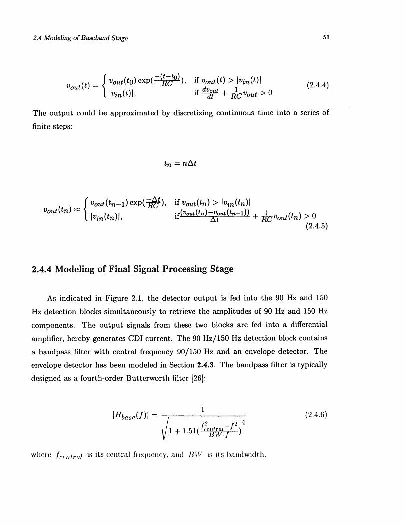
v0111() Vuit(t 0)cxp(VOI~ { Ivin(Ol)I,if vout(t) > Ivin(t)lif vo + •Vout > 0
The output could be approximated by discretizing continuous time into a series of
finite steps:
tn = nAt
t V(( out(tn-1) exp( -), if vout(tn) > Ivin(tn)lf(vout (tn) -Vout (tn-)) + E vo u t (t n ) > 0
(2.4.5)
2.4.4 Modeling of Final Signal Processing Stage
As indicated in Figure 2.1, the detector output is fed into the 90 Hz and 150
Hz detection blocks simultaneously to retrieve the amplitudes of 90 Hz and 150 Hz
components. The output signals from these two blocks are fed into a differential
amplifier, hereby generates CDI current. The 90 Hz/150 Hz detection block contains
a bandpass filter with central frequency 90/150 Hz and an envelope detector. The
envelope detector has been modeled in Section 2.4.3. The bandpass filter is typically
designed as a fourth-order Butterworth filter [26]:
IHbase(f)l =
1I+i f2 4)
wllere f(.(lt?.,rl is its central frequllency, and 1311' is its bandwidth.
(2.4.4)
(2.4.6)

Chapter 2 Generic Model for ILS Receiver
Similar to Section 2.4.3, all the signal flow is simulated in discrete level. The
simulation processes are arranged in this way:
1. Convert the discrete-time input signal (see (2.4.5)) into frequency-domain signal.
2. Multiply it with 90 Hz bandpass filter response Hbase(f) (see eqno(2.4.6)).
3. Inverse transform the resultant frequency-domain signal into time domain.
4. Pass through the envelope detector. Use (2.4.5) to evaluate the output.
5. Repeat (2) to (4) for 150 Hz portion.
6. Pass the results obtained from (4) and (5) into a differential amplifier to obtain
the difference. Multiply it by a constant gain. Take time average of the result to get
CDI output.
2.4.5 Approximation Scheme of IF Envelope Detector
The input of IF envelope detector (denoted by i,,(t)) contains IF localizer
signal and IF noise (denoted by N fM(t) ) with the specific average power spectrum
(as indicated in Figure 2.10),
(t) = A IF[1 + Trg9 0 cos(2r -90t) + t 1L50 cos(27r - 150t)] cos(27rfIFt) + NI (t)

2.4 Modeling of Baseband Stage
The function of envelope detector model is to simulate the output temporal signal
zout(t) in response to the input xin (t). As described in Section 2.4.3, the operation of
an envelope detector can be numerically simulated by using finite-difference method.
The IF envelope detector receives IF localizer signal and noise and converts them
into the baseband. In order to avoid under-sampling the sampling rate should be
comparable to fIF (or even higher since the interference contains higher frequency
components). For a fixed total simulation duration T, the number of time steps for
a single realization is -. O(T - fIF). The total simulation duration T is related to
the frequency resolution. It should be longer than one period of 90 Hz ( 0.011sec).
fIF is in the order of MHz. In sixth-order Chebyshev model it is 30.5 MHz. So the
number of time steps, if estimated practically, is about the order of 106. A lot of
computation time should be spent on simulating envelope detector.
An approximation scheme can be used to reduce computational complexity of
direct simulation on envelope detector. The rationality of this scheme is that by
replacing the original IF interference with a baseband interference at input, we can
get approximately the same output. And the computational complexity of envelope
detector simulation in response to this new input is much lower since the input has a
much smaller bandwidth. The method is depicted as follows.
Define a baseband noise Nbase(t) such that
NIMF(t) = NIM (t) - 2 cos(27rfIFt)
The Fourier transform of a time-domain signal x(t) is denoted by xF(f). It is
obvious that the spectrum of baseband noise Nbse is a direct translation of IF noise
spectrum.
IF f) bas ase (2.F
NIMIF(= NIAt F(f - f( F) + NI •! F(f + fIF) (2.7)
Now define a new inllut x*:r(t) to the samIie envClopC detector. It. contaills l)asc)ill(ld
localizer signal and btaselani noise,

Chapter 2 Generic Model for ILS Receiver
(t)= AIF + 0 cos(2r -90t) + ml150 cos(2r - 150t)] + Nb e(t)
The average power spectrum of Nbase and baseband localizer are demonstrated in
Figure 2.10 Denote the envelope detector output in response to xin(t) as Xout(t )
Then xout(t) z out(t) if the relaxation time of envelope detector is much longer
than the period (or the duration when signal level approaches but not exactly equals
to original values, i.e. quasiperiod) of Xin(t)*. The reason is obvious: Xn(t) is the
envelope of Xin(t), and xut(t) is the envelope of x• (t); if detector's relaxation time
is too long to follow the variation of xin(t), then the envelope of Xin(t) 's envelope
will be detected at output. Under this approximation, the sampling rate that could
recover characteristics of baseband signal xin(t) is adequate. Therefore it is in the
order of baseband noise bandwidth BW. The number of time steps ~ O(T- BW).
Compared with direct simulation, it would save computation time with the ratio
(4•) . The FM bandwidth BW is usually tens of KHz. So the computational
complexity is reduced by three orders of magnitude compared to the original scheme.
The validity of this approximation scheme could be illustrated by comparing the
direct simulation results with approximated simulation results.
pure carrier pure carrier
<INbase (f 2 > 90 Hz subcarrier< NIF(f2
150 Hz subcarrier90 Hz subcarrier
150 Hz subcarrierit \t-00-
Fig2.10 IF and baseband noise s)pectrull(one side)
0 flF
N--BW - d- RW ---

2.4 Modeling of Baseband Stage
In the following paragraph we conduct numerical simulation on baseband stage
( including envelope detector ) to show that our approximation scheme is valid.
The baseband receiver parameters and other simulation conditions are described as
follows:
Receiver Parameters:
IF center frequency : flF = 30.5 MHz
IF envelope detector bandwidth: 500 Hz
IF reference voltage level: Vref = 0.212V
90/150 Hz filter bandwidth: BWbase = 30 Hz
90/150 Hz filter gain: Ag9 = 1.0, A 150 = 1.021
90/150 Hz envelope detector bandwidth: 10 Hz
differential amplifier gain: Ad = 4.96
output impedance: Ro = lkQ
Simulation Conditions:
noise bandwidth: BWN = 64.0 KHz
simulation period T = 0.1 sec
number of IF noise levels bl)t,ween and 100% noise: 50
number of samiples for IF-cnvclope-detcctor simulattion: 3072000
number of samlllles for basel)anl( simulation: 10241
Chapter 2 Generic Model for ILS Receiver
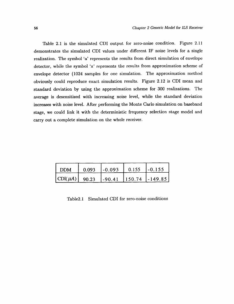
Table 2.1 is the simulated CDI output for zero-noise condition. Figure 2.11
demonstrates the simulated CDI values under different IF noise levels for a single
realization. The symbol 'a' represents the results from direct simulation of envelope
detector, while the symbol 'x' represents the results from approximation scheme of
envelope detector (1024 samples for one simulation. The approximation method
obviously could reproduce exact simulation results. Figure 2.12 is CDI mean and
standard deviation by using the approximation scheme for 300 realizations. The
average is desensitized with increasing noise level, while the standard deviation
increases with noise level. After performing the Monte Carlo simulation on baseband
stage, we could link it with the deterministic frequency selection stage model and
carry out a complete simulation on the whole receiver.
Table2.1 Simulated CDI for zero-noise conditions
DDM 0.093 -0.093 0.155 -0.155
CDI(pA) 90.23 -90.41 150.74 -149.85

2.4 Modeling of Basebaind Stage
CDI output from baseband stage
ILU
110100908070
605040
302010n
0 0.04 0.08 0.12 0.16 0.2
IF noise level(V)
Fig2.11 CDI output based on simulated and approximated envelope detector
CDI output from baseband stage
1 2 0 ......... ................. .........110 Mean
- - - Standard deviation100
908070605040
302010 ---
0 AJLA A-L1I.LL IJ4.J IAJlW~ALL
0 0.04 0.08 0.12 0.16 0.2
IF noise level(V)
Fig2.12 Cl)l iean and standard deviation
v

Chapter 3 Model Synthesis
Chapter 3
Model Synthesis
3.1 EXPERIMENTS FOR ILS RECEIVER INTERFERENCE
In order to understand ILS localizer receiver's susceptibility to interference,
Federal Aviation Administration (FAA) and other civil aviation authorities conducted
a series of bench tests over different kinds of receivers. The focus is to measure the
'threshold' of input interfering power; that is, for a certain localizer power level
and a set of interfering frequencies, to what extent the input interfering power
should reach in order to cause 'intolerable' CDI error. FAA and International
Telecommunication Union (ITU) have developed different regression formula to
describe these experimental data in different perspective. These formula serve as
reference of theoretical model proposed in Chapter 2: simulation results from a correct
model should fit experimental data.
The standard experimental procedures for two-frequency intermodulation (B131)
interference of ILS localizer receivers could be outlined as follows. Figure 3.1 is the
corresponding equipment setup for two-frequency Bi experiments.
1. Use localizer simrulator to generate localizer sigiial with clloseii carrier
freqiuency floc and(l power level (e.g. -86 dBmn). Pick iup a type of localizer receivcr
set.. Inlject localiz(er signal into localizer receiver and i rcadl CI)I ciirrienlt valuti. Adjuist.
D)I)MN1 value until 90 ILA C)1 curr.ent, is read.

3.1 Experiments for ILS Receiver Interference
CDI = 90uA CDI = 90GMA ± error
erf2
Fig3.1 Experimental setup for ILS Bl-interference tests
Reference: Test Condition:
0

Chapter 3 Model Synthesis
2. Use noise simulator and frequency modulator to generate FM noise with
carrier frequency fl . The other interference component is FM without audio message
(i.e. a pure carrier) with chosen frequency f2- fl and f2 are chosen to satisfy
intermodulation condition 2fl - f2 = floc. Feed both components into receiver.
Their power levels are set equal all the time. The level is called equisignal level.
3. At a fixed interference power level, CDI output is not always at constant
level but fluctuates with time. Write down all the CDI sample values at that level.
Do statistical analysis on those sample data to see if the statistical outcomes meet
the threshold condition. If not, increase input interference power level by 1-dB
step and repeat the process until threshold condition is reached. The corresponding
equisignal level is defined as the 'threshold' of input interference power. Write down
the threshold value. The threshold conditions for different models are different. For
AAM the threshold is defined as the condition when 10% of CDI sample values fall
out of (90 ± 9)pA (i.e. > 99pA or < 81/A). For ITU model if the CDI standard
deviation exceeds 2.25 pIA then threshold is reached.
4. Change different FM channels fl f2 that satisfy intermodulation condition.
Carry out 2 to 3. Get threshold values corresponding to different frequency
combinations.
5. Change localizer power to different levels (e.g. -49dBm, -67dBm). Repeat 1
to 4.
6. Repeat procedures 1 to 5 for different types of localizer receiver sets.

3.1 Experiments for ILS Receiver Interference
IM threshold varies with input interfering frequencies. In two-frequency Bi case
IM threshold is a function of fl and f2. However, casting the experimental outcome
into multi-dimensional domain would make regression analysis more complicated.
From statistical analysis of experimental data, it was found that the most relevant
single variable to IM threshold is the product of separation between localizer and
interfering frequencies (floc - fl)(floc- fl)(floc - f2)- So the FAA and ITU
represent IM threshold as a dependent variable of only one independent parameter
which measures the frequency separation. For two-frequency IM case it is defined
this way:
AAM Model:
ga = log (floc - fl)(floc - f)(floc - f2) (3.1.1)
ITU Model:
git = log JIMax(l.O, fioc - fl)Max(l .0 , floc - fl)Max(l .0 , floc - f2)1 (3.1.2)
where all frequencies are in MHz unit.
The experimental procedure for three-frequency intermodulation interference is
almost the same as two-frequency except three different noise sources with frequencies
fl, f2, f3 (one is FM, the other two are pure carriers) satisfying intermodulation
condition are fed into localizer receiver. The definition of g for AAM and ITU models
are similar t.o (3.1.1) and (3.1.2) except an fl is replaced by f3.
Chapter 3 Model Synthesis
Loc power=-86dBm
E
().
7)3
W-CCn
10:
0
-10
-20
-30
-40
-2 -1 0 1 2 3
g=log((fl -floc)*(f2-floc)*(f2-floc))
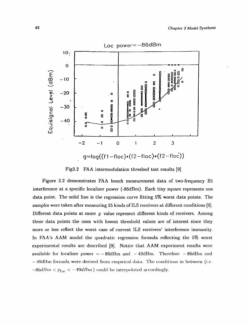
Fig3.2 FAA intermodulation threshed test results [9]
Figure 3.2 demonstrates FAA bench measurement data of two-frequency Bi
interference at a specific localizer power (-86dBm). Each tiny square represents one
data point. The solid line is the regression curve fitting 5% worst data points. The
samples were taken after measuring 25 kinds of ILS receivers at different conditions [9].
Different data points at same g value represent different kinds of receivers. Among
these data points the ones with lowest threshold values are of interest since they
more or less reflect the worst case of current ILS receivers' interference immunity.
In FAA's AAM model the quadratic regression formula reflecting the 5% worst
experimental results are described [9]. Notice that AAM experiment results were
available for localizer power = - 86dBmi and - 49dBm. Therefore - 86dBm and
- 49d(B113n formula were derived from enipirical data. Thle (:cond(litions in between (i.e.
-86dlhn < Plc < -- 49dBm ) coul(l l)e int.erpolat.e(l accordingly.

3.1 Experiments for ILS Receiver Interference
Th(ga, -86) = -40.2590 + 2 .9 7 2 8ga + 1.6895g2
Th(ga, -49) = -18.1980 + 2.0070ga + 1.0596ga
Th(ga, Ploc)1
= -(Th(ga, -49) - Th(ga, - 8 6 ))(ga + 86)37
+Th(ga, -86)
AAM Three Frequencies:
(3.1.5)
(3.1.6)Th(ga, -86) = -40.1634 + 2 .19 7 7 ga + 1.5668g 2
Th(ga, -49) = -18.9296 + 1.0941ga + 1.2215g 2 (3.1.7)
Th(ga, Ploc) = Th(ga, -86)+
-(Th(ga, -49) - Th(ga, -86))(ga + 86)37
(3.1.8)
The unit of Th(.,.) and ploc is dBm. ga is calculated from (3.1.1)
I'TU lmodel lhas differenlt regression formula [3]. Tile equisignal threshold is linear
wit.h both g and localizer power. The depend(ence of localizcr power is also included
ill tllew forullla.
AAM Two Frequencies:
(3.1.3)
(3.1.4)

Chapter 3 Model Synthesis
ITU Two Frequencies:
282= g- 513
+ Ploc3 (3.1.9)
ITU Three Frequencies:
Th(git, ploc) =2828 git - 533
Ploc3 (3.1.10)
The unit of Th(., .) and ploc is dBm. git is calculated from (3.1.2)
3.2 MODEL SYNTHESIS-INVERSION OF RECEIVER PARAME-TERS
Chapter two gives a detailed description of ILS generic receiver model. This
model is generic in the sense that it is characterized by a set of receiver parameters.
The receiver parameters are listed below:
Frequency Selection Stage:
Front End: equivalent input impedance Rin
RF: APreRF' KRF , KRF, Apot Hpost(f)1 F 3 R' IRF
Mixer: K•Z ix , K4Mix
Local oscillator output: frequency fos c, amplitude Aose
I 4 1 3IF: t (f)t v Kge Klevel:
IF output voltage level: V0
jj~ 7t (j)
Th(git, Ploc)

3.2 Model Synthesis-In version of Receiver Parameters
Baseband Stage:
IF envelope detector: time constant tlF
90/150 Hz Bandpass filter: bandwidth BW9 0 / BW 150 , gain A9g / A1 50
90/150 Hz envelope detector: time constant t90 / t 150
differential amplifier: gain Ad, impedance Rd
In this model the determination of baseband-stage parameters is based on the
criterion mentioned in Section 2.4.2: baseband simulation model should satisfy the
proportional condition - if DDM= d corresponds to CDI= cp A then DDM= -d
corresponds to CDI= -cpi A; as well as the maximal deviation condition - DDM=
0.0155 corresponding to 150 pA CDI current. The former could be achieved by
adjusting the ratio BW 9 0 /BW 15 0 and A 90 /A 150 . The later could be achieved by
adjusting others. However, the two conditions do not uniquely determine the value of
every baseband parameter. In realistic situation these values, depending on different
circuit designs, vary from one to another type of ILS receivers. We assign these values
such that they approximately fit the scale of real receiver circuits.
Unlike baseband parameters which are determined by the response to pure local-
izer signal, frequency-selection stage parameters could be inverted from experimental
results. Setting the input interference power at the equisignal threshold, we can sim-
ulate the receiver response. The total (third-order)IM power depends on RF filters
response A ,F' HW'(f), Ap't, H o t (f), as well as RF amplifier (third-order)
K3F KMixnonlinearity , and balanced mixer (fourth-order) nonlinearity . Note the2
local oscillator output voltage Aosc. and input impedlance Rin also have effects since
the former is relat.ed to the value of mixer nonlinearity (see (2.3.7)) and the latter
transfers power level into voltage level. The( regressioll culrves of AAM, ITU and
ICA() miiodels l)rovi(de the lower bountd for the IM interference imnmunity of ILS re-
ceivers. If we could find out a set. of p)arallleter values that, fit, simulation result's with

Chapter 3 Model Synthesis
empirical regression curves, then these values are considered a characterization of ILS
localizer receivers. The set of parameters corresponding to AAM regression curves is
the representation of so-called "AAM receiver", and the set corresponding to ITU or
ICAO regression curves is the representation of so-called "ITU receiver" or "ICAO
receiver".
This inverse problem could be formulated as a least-square optimization problem.
Parameters are denoted by a vector b = (b1 , b2 , ..., bM). Input quantities are denoted
by x = (g, Ploc)" There are N different sampling points related to N different
input conditions x,, x2, .... ,xN. The threshold value corresponding to input xi is
Yiref from regression formula, and is yi from theoretical model. yi is a function
of receiver parameters, yi = Yi(b) . The inverse problem is to find out a parameter
vector bo such that the distance between empirical and theoretical results, defined
as E 1 yref - Yi(bo) 2 , is minimal. In another word, let Y = (YlY2, .,YN),
yref = (yref ,ef y ef), the problem is to find out b0 such that the objective
IIY(bo) - Y*112 is minimal.
The input variable g is actually a specification of input interfering frequen-
cies. For two-frequency intermodulation case, the input frequencies are uniquely
determined by g, for three-frequency intermodulation case they are not uniquely
determined. The inversion scheme adopts regression formula of two-frequency B1 as
reference to inverse receiver parameters. The parameters to be inverted and input
conditions designated in our inversion scheme are depicted below:
Inverted Parameters:
R i A- pr, Hpre (f KMix KMix, AoscKI /' R lF' =RFf/' / , os
K3RFr/K•F(Ploc = -86NdBrn), K R F 1 K R r (P = -67dI37n),3 3 / 1 lo
K(1?/Kf/(()1oc = -49dBr) , KMijlx/K lirX , Aosc
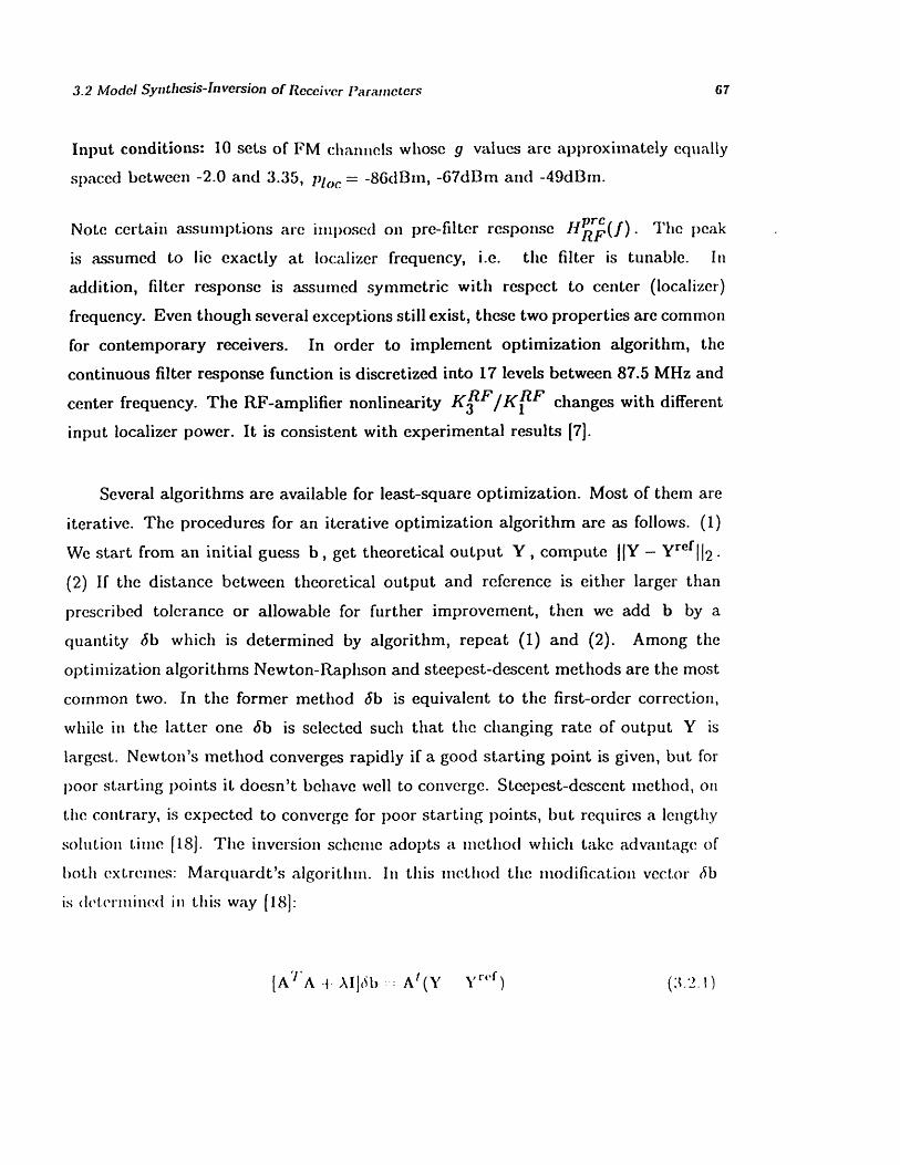
3.2 Model Synthesis-In version of Receiver Parameters
Input conditions: 10 sets of FM channels whose g values are approximately equally
spaced between -2.0 and 3.35, poc = -86dBin, -67dBm and -49dBm.
Note certain assumptions are impll)osed on pre-filter response HR(f). The peak
is assumed to lie exactly at localizer frequency, i.e. the filter is tunable. In
addition, filter response is assumed symmetric with respect to center (localizer)
frequency. Even though several exceptions still exist, these two properties are common
for contemporary receivers. In order to implement optimization algorithm, the
continuous filter response function is discretized into 17 levels between 87.5 MHz and
center frequency. The RF-amplifier nonlinearity KgRF/KIRF changes with different
input localizer power. It is consistent with experimental results [7].
Several algorithms are available for least-square optimization. Most of them are
iterative. The procedures for an iterative optimization algorithm are as follows. (1)
We start from an initial guess b, get theoretical output Y, compute IlY - yrefil2 .
(2) If the distance between theoretical output and reference is either larger than
prescribed tolerance or allowable for further improvement, then we add b by a
quantity 6b which is determined by algorithm, repeat (1) and (2). Among the
optimization algorithms Newton-Raphson and steepest-descent methods are the most
common two. In the former method Jb is equivalent to the first-order correction,
while in the latter one 6b is selected such that the changing rate of output Y is
largest. Newton's method converges rapidly if a good starting point is given, but for
poor starting points it doesn't behave well to converge. Steepest-descent method, on
the contrary, is expected to converge for poor starting points, but requires a lengthy
solution time [18]. The inversion scheme adopts a method which take advantage of
bothi extremes: Marquardt's algorithmln. In this method the modification vector (5b
is etermllined in this way [18]:
[A"'A + Al]h t ( A t ( Y Y"rf) (3. 2.1 )

Chapter 3 Model Synthesis
A is an N x M matrix with element Aij - . A T is A 's transpose matrix. I
is an N x N identity matrix. A is a correction factor. It can be shown that when
A = 0 Marquardt's algorithm becomes Newton's miethod, when A = oo it becomes
steepest-descent method. Thus in Marquardt procedure the initial values of A are
large and will decrease toward zero as the optimum is approached.
Figure 3.3 is a diagrammatic representation of model synthesis procedures. By
the accomplishment of these procedures we should be able to invert AAM, ITU and
ICAO receivers.
,Pi)
out[)tut X
ig3 3 1i;r eter ini versio)Ii Icoc ires

3.3 Inverted Receivers and Threshold Curves
3.3 INVERTED RECEIVERS AND THRESHOLD CURVES
The inverted results are demonstrated as follows. Figure 3.4 and 3.5 are pre-
filter's frequency responses of inverted AAM and ITU receivers. Table 3.3 lists the
values for the other inverted AAM and ITU receiver parameters. These parameter
values are obtained by optimizing simulation results to empirical data for two-
frequency regression curves at localizer power levels -86dBm, -67dBm and -49dBm.
Figure 3.6 and 3.8 demonstrate the simulated as well as regression two-frequency
B1 threshold curves for AAM and ITU models. If the derived model is self-consistent,
the simulation results should also fit empirical data well for other intermodulation
conditions. Figure 3.7 and 3.9 demonstrate the simulated as well as regression three-
frequency B1 threshold curves for AAM and ITU models. Both two-frequency and
three-frequency curves represent finite numbers of frequency combinations. The pairs
chosen for two-frequency and three-frequency intermodulation are listed in Table 3.1
and 3.2. The localizer frequency is 108.1 MHz.
As indicated in Figure 3.6 and 3.7, the AAM simulation results deviate more
from regression curves when interfering frequencies are close to localizer frequency.
From the quadratic regression formula the value increases as frequency separation
decreases in this region. On the other hand, receiver model predicts monotonically
decreasing when filter responses are monotonic. This discrepancy, in additional to the
incompleteness of receiver model or inversion scheme, may be derived from the way
AAM empirical formula are developed. AAM formula correspond to the regression
of performance among 5% worst receivers. However, the numbers of receivers under
test are not all the same for different frequency pairs. There are fewer data points
whlien is extremely low or high (see Figure 3.2). The 5% lowest data points at low
y -values (e.g. g < -1.0 in Figure 3.2) may not rep)resent the same kinds of receivers
as those at nlormlal g -values. Tlheir t.hlreshold( equisignal levels at highler g -values
may be higher thlman 5% worst cases.

Chapter 3 Model Synthesis
fl(MHz) 107.9 107.7 107.5 107.3 107.1
f2(MHz) 1107.7 107.3 1 106.9 106.5 1 106.1
Ifl(MHz) 106.5 105.5 103.9 101.5 98.1f 2(MHz) 104.9 102.9 99.7 94.9 88.1
Table3.1 Intermodulation frequencies(two frequencies)
fl(MHz) 107.9 107.9 107.9 107.9 107.7
f 2(MHz) 107.7 107.5 106.7 106.1 105.3
f 3(MHz) 107.5 107.3 106.5 105.9 104.9
fi(MHz) 107.3 105.9 104.3 102.7 102.1
f2(MHz) 104.7 103.9 103.5 100.5 94.1f3(MHz) 103.9 101.7 99.7 95.1 88.1
Table3.2 Intermodulation frequencies(three frequencies)
Model AAM ITU
Ri,, (KO) 82.22 99.91A Pr
RF 0.3 0.8
K'F I K F(-8 6 dBm) 1.266 1.333RF RFK3 / K, (-67dBm) 0.949 1.167
K3F / K F(- 4 9dBm) 0.522 1.000
A,S,. 0.283 0.600
K""'r / K"' •" 0.310 0.259
Tablc3.3 Inverted receiver p)arameters
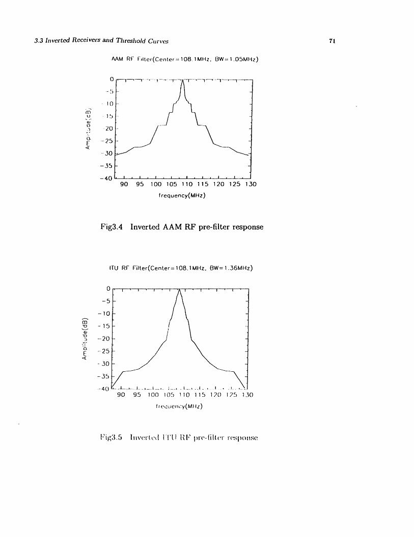
3.3 Inverted Receivers and Threshold Curves
AAM RF Filter(Center- 108.1 MHz. 3W= 1 .05MHz)
--5 t
10
1 .)
20
-25
-30
-35
-4090 95 100 105 110 115 120 125 130
frequency(MHz)
Fig3.4 Inverted AAM RF pre-filter response
ITU RF Filter(Center= 108.1 MHz. BW=1.36MHz)
-5
-10
-15
-20
-25
- 30
-35
-4090 95 100 105 110 115 120 125 130
frecuency(Mflz)
I'ig:3.5 lnverYt.el IT'il Ri' plre-(iler rceslOIlse
I'A
r,-
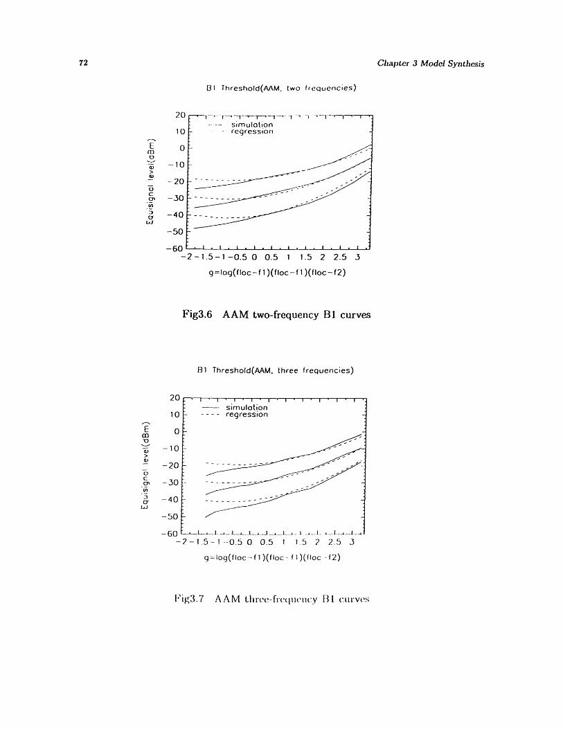
Chapter 3 Model Synthesis
631 Threshold(AAM. two frequencies)
1CC
-10
- 20
-30
-40
-50
-F;n-2-1 .5-1 -0.5 0 0.5 1 1.5 2 2.5 3
g=Iog(floc-f 1)(floc-f 1 )(floc-f2)
Fig3.6 AAM two-frequency BI curves
B1 Threshold(AAM, three frequencies)
I I'I' Isimulotion
- regression
-2-1.5-1 --0.5 0 0.5 1 1.5 2 2.5 3
g =log(floc--fl)(floc- f 1l)(floc -f 2)
!'ig3.7 AAM4 I.ree-frcIeluiency 1l1 curv~es
0
-10
-20
-30
-40
-50
-60
------------
-----------
L1~..1. _1~_ I__.i.__L_.I___1 _4._1.__1._ i ~1_.~1~ 1.~~ 1._~1.~.

3.3 Inverted Receivers and Threshold Curves
31 Threshold(ITU. two frequencies)
simulation-- regression
-2-1.5-1-0.5 0 0.5 1 1.5 2 2.5 3
g=log(floc-f1 )(floc-f 1 )(floc-f2)
Fig3.8 ITU two-frequency Bl curves
B1 Threshold(ITU. three frequencies)
--2-1.5-1-0.5 0 0.5 1 1 5 2 2.5 3
g log(floc- (1)(floc -- 1)(floc- -2)
I"ig3.9 1'*I'1..J tIIr('c- II('(f1I&'IIU~' I I (1V('M
'U
10
0
--10
-20
-30
-40
-50-60
20
10
0
-10
-20
- 30
-40
-50
-fA
zu
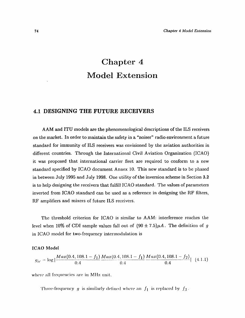
Chapter 4 Model Extension
Chapter 4
Model Extension
4.1 DESIGNING THE FUTURE RECEIVERS
AAM and ITU models are the phenomenological descriptions of the ILS receivers
on the market. In order to maintain the safety in a "noiser" radio environment a future
standard for immunity of ILS receivers was envisioned by the aviation authorities in
different countries. Through the International Civil Aviation Organization (ICAO)
it was proposed that international carrier fleet are required to conform to a new
standard specified by ICAO document Annex 10. This new standard is to be phased
in between July 1995 and July 1998. One utility of the inversion scheme in Section 3.2
is to help designing the receivers that fulfill ICAO standard. The values of parameters
inverted from ICAO standard can be used as a reference in designing the RF filters,
RF amplifiers and mixers of future ILS receivers.
The threshold criterion for ICAO is similar to AAM: interference reaches the
level when 10% of CDI sample values fall out of (90 ± 7.5)ILA. The definition of g
in ICAO model for two-frequency interinodulation is
ICAO Model
log Max(0.4, 108.1 - fl) Max)(0.4, 108.1 - fl) Mal:(0.4, 108.1 - f2)y . = lo' | | (41.1.1)().4 0.4 0.4
where all frequencies are ini MHz unit.
'l'lhree-frequency g is similarly detinled where all fl is repllaced by f'3-

4.1 Designing the Future Receivers
ICAO curves are similar to their counterparts of ITU regression curves:
ICAO Two Frequencies:
20Th(gic, Ploc) = -ic + 12.625467 + (4.1.2)
ICAO Three Frequencies:
20Th(gic, ploc) = gic + 10.625467 + Ploc
3 (4.1.3)
Figure 4.1 is pre-filter's frequency responses of inverted ICAO receiver. Table
4.1 lists the values for the other inverted ICAO receiver parameters. Notice that
compared with Table 3.3 ICAO standard could be achieved by desensitizing RF
input 26.03 dB with respect to ITU. If we don't resort to this approach but only
to sharpen the filter response or to lessen the coefficient of third-order nonlinearity
or to both we could still get ICAO receiver. But the filter or amplifier would go far
beyond the realizable ranges. Therefore from an engineering point of view RF input
desensitization is a sensible design for the fulfillment of higher interference-immunity
standard. The reason for it is obvious. Suppose the input localizer level is Alo c ,
and input noise levels for three channels are N 1 , N 2 , N3 (all in dB scale). The
intermodulation level would be N 1 + N2 + N3 - (filter effect). Now the RF input
is desensitized by a coefficient A, then localizer level becomes Aloe - A, while the
intermodulation level becomes N 1 + N2 + N3 - 3A- (filter effect). The (4) ratio
improves 2A than original one. So intermodulation interference is better suppressed.
1Figure 4.2 dehmonstrates the silmulatedl as well as regression t.wo-fr(lIequency 131
thiresldohi cuirves for ICAO() iodel. Figure -1.3 cellonstrates tile siIlllatedl as well Ias
regression three-frequiellcy 131 thiresholdlh cir-ves for ICAO miodel. The input.t, friequency
pairs choseil for two-frequency aiidl t.lree-ftreq(iemcy interimoldulation1 are samle as those
in Tabhle 3.1 and 3.2. I'lThe localizer 'freqmen.cy is 108.1 MIIz.

Model
R,, ( K )
A reRF
K3R" I K RF(.-86dBm)
K F I K RF ( - 6 7 d B m )
KRF / KF (-49dBm)
A oC
KxN' / K •̀4 2
ICAO
82.22
0.04
1.266
0.949
0.522
3.283
0.310
Table4.1 Inverted ICAO receiver parameters
ICAO RF Fifter(Center= 108.1 MHz. BW= 1.04MHz)
-10
-15
-20
-25
-30
-35
-4090 95 100 105 110 115 120 125 130
frequency(MHz)
Fig4.1 Inverted ICAO RF pre-filter response
Chapter 4 Model Extension
I

4.1 Designing the Future Receivers
B1 Threshold(ICAO. two frequencies)
10 - --. regression -
10
- 10 -
-- 20
-30
-40
-50
-6 A..f)~~t-2-1.5-1-0.5 0 0.5 1 1.5 2 2.5 3
g=log(floc- f 1)(floc- f 1 )(floc-f2)
Fig4.2 ICAO two-frequency B1 curves
81 Threshold(ICAO. three frequencies)
"9/'0
10
0
-10
-20
-30
-40
-50
-ýn-2-1.5-1-050 0.5 1 1.5 2 2.5 3
g= -og(floc -- f 1)(floc -fl )(iluc -f2)
l"ig4.3 ICA() .iree-frequeicY 131 curves
20simulation

Chapter 4 Model Extension
4.2 PURE-CARRIER INTERMODULATION INTERFERENCE
The extent of pure-carrier intermodulation interference is also of concern to the
aviation communities. In order to certify a new receiver radio interference immunity
needs to be treated on pure-carrier noise as well as FM noise. It is observed that
intermodulation interference from pure carrier might be more serious than that from
FM. The simulation procedures are exactly the same as those of Section 4.2 except
the noise spectrum mentioned in Section 2.4.2 is replaced by a single component.
Notice even though pure carrier, unlike FM noise, has a deterministic spectrum,
Monte Carlo simulation is still required since the relative phase of noise carrier with
respect to localizer carrier is a random variable. Figure 4.4, 4.5 and 4.6 compare the
two-frequency threshold curves for pure-carrier noise with those for FM noise. Even
though the total power of pure carrier locates out of both the 90 HZ and 150 Hz filter
passband, this comparison shows that pure-carrier intermodulation interference is at
least as serious as FM intermodulation interference. In AAM and ITU models the
former ones are even more serious. It is because the impact of interference cannot be
comprehend as direct 'leaking' to baseband stage but involves the envelope extraction
which in itself is a nonlinear operation.

4.2 Pure-Carrier Intermodulation Interference
(31 Threshold(AAM. two frequencies)
0
-- 10
--20
--30
-40
-50
-fn
-2- 1.5-1 -0.5 0 0.5 1 1.5 2 2.5 3
g=Iog(floc-f 1 )(floc - f 1 )(floc-f2)
Fig4.4 Comparison of pure-carrier interference with FM interference: AAM model
81 Threshold(ITU. two frequencies)
10
0
-10
-20
-30
-40
-50
- (;o
Pure carrier
-2--1.5 -1 -0.5 0 0.5 1 1.5 2 2.5 3
g=-Iog(floc--f 1)(floc f 1)(floc--12)
I"ig.1r.5 (, illiarisoI of iirre1-carrier iinterfernce wit. ' IMI iiniterference:I l'lT I1odelc

Chapter 4 Model Extension
B1 Threshold(ICAO. two frequencies)
0
-10
-20
-30
-40
-50
-FO-2-1.5-1 -0.5 0 0.5 1 1.5 2 2.5 3
g=log(floc-f 1 )(floc-f 1 )(floc-f2)
Fig4.6 Comparison of pure-carrier interference with FM interference: ICAO model

4.3 Calculation of Course Deviation Current
4.3 CALCULATION OF COURSE DEVIATION CURRENT
The function of this model is to calculate CDI under various interference
conditions, including both threshold and non-threshold. By using this model as a
tool the simulation on aircraft landing process could be carried out.
Since the noise assumed in this model is stochastic, CDI value is also non-
deterministic. We could simulate its statistical behavior. Take AAM receiver as
an example. Figure 4.7 is the simulated AAM threshold curve at localizer power
-86 dBm and frequency 108.1 MHz. Icons 'A', 'B', and 'C' represent over-threshold
(noise power -- 37 dBm), threshold (noise power -39 dBm) and under-threshold
(noise power - 41 dBm) conditions when a specific intermodulation pair is selected
(fl = 107.1 MHz, f2 = 106.1 MHz). Figure 4.8 to Figure 4.10 represent CDI
distribution under condition 'A', 'B' and 'C'. The number of realizations is 200.
81 Threshold(AAM. two frequencies)
-z
-30
-40
-50o -LJa
.-•t
-2-15--1-0.50 05 5 1 5 2 2.5 3
q Ioq(floc--f )(flo" 'I )it'oC f 2)
l'igl.7 Specif ic(al.i() (of over-t.hreslhold, thiresihold aid( III (ler-t.lhreshold col(it. ioIS

82 Chapter 4 Model Extension
CDI Di.strbut.on(nos - -3 7dcU[l A)
0 25
02
0 15
0.05 * *
40 50 60 70 80 90 100 110 120
CDO(uA)
Fig4.8 CDI distribution(over-threshold): mean=78.01 I A, deviation= 13.66z A
CDI D;stributlion(noise--39d8m. 8)
O.3
0.25
0.2
o 0.15
0.1
0.05
40 50 60 70 80 90 100 110 120
CDI(uA)
Fig4.9 CDI distribution(threshold): mean=84.77 p A, deviation=6.90 p A
CDI 0.stribution(nose= -4 IdBm C)
o03
0.25
02S 0.15
01
0 05
4) 50 60 70 80 90 100 r10 tO20
"igl.10 (CI)1 (istriit. i( der-t .reshl)() mean= 88.53 p A, d(eviatioll - 3.5 I pA

Chapter 5
Conclusion
This thesis proposes a stochastic ILS localizer receiver simulation model to
estimate CDI output values given the power and frequencies of localizer signal and
noise components. It is achieved by parametrizing each stage in an ILS receiver,
including RF section, mixer, IF section, automatic gain control, IF envelope detector
and 90/150 Hz detection stage. The nonlinear characteristics of RF amplifier,
mixer and IF amplifier is approximated by a third-order polynomial. All receiver
characteristics are parametrized, and the values of parameters are inverted by
fitting simulation results with AAM, ITU and ICAO curves for a chosen test
condition. The inverted receiver model could be verified from other test conditions.
Simulation results fit empirical data well for three-frequency, pure-carrier and fifth-
order intermodulation conditions. It is an indication that our generic model could
capture the performance of ILS localizer receivers. For brute-force interference,
simulation results indicate that intermodulation and AGC may not be the principal
causes. Other nonlinear mechanism, such as clamping effect at front end, may take
the responsibility for interference at high input noise level.
Chapter 5 Conclusion
The purpose of this research is embedded in a broader scenario: the overall
simulation of the aircraft landing process under the realistic radio environment. The
combination of receiver model with aircraft aerodynamic model, aircraft control
law model, EM propagation model and the database of the position, power,
frequency of ILS localizer and FM stations offer a tool for the simulation of aircraft
landing trajectory. The statistics obtained from Monte Carlo simulation on landing
trajectories such as failure rate provides a clear reference of automatic landing
system performance within a specific geographic region. A complete receiver is an
indispensible part of the overall system evaluation model.
The ILS localizer receiver model is still far from comprehensive. Several issues
are important for the achievement of a more accurate model in the future. Fifth-
order intermodulation effect should be considered when input noise power is relatively
higher than that at third-order threshold level. The immediate modification is
replacing the transfer function of nonlinear amplifier, y = K 1 x + K 3 x 3 , by y =
K l x + K3 x3 + K 5 x 5 . And the fifth-order intermodulation is generated by the fifth-
order harmonic K 5 x 5 . But more complication is involved for the contribution of
intermodulation power when more than one nonlinear stage are connected. It requires
more theoretical and simulation works. In addition, intermodulation cannot explain
the brute-force(B2) interference. It is generally believed that brute-force interference
happens because the high noise power level desensitizes the receiver thus to change
localizer output. It could result from AGC desensitization - the noise power leaks
through IF filter therefore to drive AGC to reduce localizer amplitude, or from front-
stage nonlinearity - the high noise power at front stages (e.g. RF section, mixer)
drives the device into highly nonlinear region to distort baseband localizer signal. To
understand the mechanism of brute-force interference further investigation is required,
too.

Reference
[1] Bennett, W. R., " Cross modulation requirements on multi-channel amplifiers
below overload, " Bell Syst. Tech. J., Vol. 19, pp. 587-610, 1940
[2] Bose, K. W., Aviation Electronics, Indiana: Howard W. Sams & Co., Inc., 1981
[3] CCIR Study Groups, Compatibility between the sound broadcasting service in the
band of about 87 -108 MHz and the aeronautical service in the band 108 -137
MHz, CCIR Draft Recommendation [F/12], 1992
[4] Chang, K. Y., " Intermodulation noise and products due to frequency dependent
nonlinearities in CATV systems, " IEEE Tran. on Comm., Vol. COM-23, No.
1, pp. 142-155, 1925
[5] Chua, L. O., Desoer, C. A., Kuh, E. S., Linear and nonlinear circuits, New York:
McGrall-Hill, 1987
[6] Edwards, R., Durkin, J., Green, D.H., " Selection of intcrmodulation-frcc
frequencies for multiple-channel mobile radio systems, " Proc. IEEE, Vol. 56,
No. 12, pp. 862-870, 1968
[7] Essiiaii, J. E., Loos, T., Analytical determCinaltlion of the intcfercfuc of
co7lmmercial FAM stations wizth airborine communicationtzhtL and navigation reccive.rs
(1and e:perimntal verzifications, FAA technical report, FAA-R-6050-1, 1978
Reference
[8] Evans, B. G., Ganem, H., " Simulation of FM/FDM blocks for interference and
interinodulation calculations, " Electro. Letter, Vol. 17, No. 25, pp. 963-964,
1981
[9] Federal Aviation Administration, User's manual and technical reference for the
airspace analysis: mathematical model, FAA Spectrum Engineering Division,
ASM-500, Version 4.1, 1992.
[10] Federal Aviation Administration, Microwave landing system demonstration
program, project summaries and MLS user financial analysis, FAA project report,
1991
[11] Gardiner, J. G., Magaza, M. S. A., " Some alternative frequency assignment
procedure for mobile radio systems, " Radio and Electro. Eng., Vol. 52, No. 4,
pp. 193-197, 1982
[12] Gavan, J., Shulman, M. B., " Effect of desensitization on mobile radio system
performance, part I: qualitative analysis, " IEEE Tran. on Vehicular Tech., Vol.
VT-33, No. 4, pp. 285-290, 1984
[13] Gavan, J., Shulman, M. B., " Effect of desensitization on mobile radio system
performance, part II: quantitative analysis, " IEEE Tran. on Vehicular Tech.,
Vol. VT-33, No. 4, pp. 291-300, 1984
[14] Gavan, J., " Main effect of mutual interference in radio communication systems
using broad-band transmitters, " IEEE Tran. on EMC., Vol. EMC-28, No. 4,
pp. 211-219, 1986

[15] Jones, J. R., Jones, S. H., Tait, G. B., Zybura, M. F., " Heterostructure barrier
varactor simulation using an integrated hydrodynamic device/harmonic-balance
circuit analysis technique, " IEEE Microwave and Guided Wave Letter, Vol. 4,
No. 12, pp. 411-413, 1994
[16] Kavehrad, M., " Multiple FM/FDM carriers through nonlinear amplifiers, "
IEEE Tran. on Comm., Vol. COM-29, No. 5, pp. 751-756, 1981
[17] Koh, P. J., Peatman, C. B., Crowe, T. W., " Millimeter wave tripler evaluation
of a metal/2-deg Schottky diode varactor, " IEEE Microwave and Guided Wave
Letter, Vol. 5, No. 2, pp. 73-75, 1995
[18] Kuester, J. L., Mize, J. H., Optimization techniques with Fortran, 1973
[19] Perlow, S. W., " Third-order distortion in amplifiers and mixers, " RCA Review,
Vol. 37, pp. 234-266, 1976
[20] Radiocommunication Study Groups, International Telecommunication Union
(ITU), Test procedures for measuring aeronautical receiver characteristics used
for determining compatibility between the sound-broadcasting service in the band
of about 87 -108 MHz and the aeronautical service in the band 108 -118 MHz,
Draft New Recommendation ITU-R [DOC.2/XX], 1995
[21] Sedra, A. S., Smith, K. C., Microelectronic circuits, New York: Holt, Rinehart
and Winston, 1982
[22] Shen, Y. C., Ton, C. P., " A scheme for further strengthening interference
protcctioll of spread spectrulI communication systems, " 1990 International
Syrmp. on EMAC, Symp. Record, pp. 532-536. 199()

Reference
[23] Simons, K. A., " The decibel relationships between amplifier distortion products,
" Proc. IEEE, Vol. 56, No. 12, pp. 862-870, 1968
[24] Stapleton, S. P., Quach, L., " Reduction of adjacent channel interference using
postdistortion, " 42th Vehicular Tech. Soc. Conference, 1992, Vol. 2, pp. 915-
918, 1992
[25] Steiner, J. W., " An analysis of radio frequency interference due to mixer
intermodulation products, " IEEE 'Tan. on EMC, Vol. EMC-6, No. 1, pp.
62-68, 1964
[26] The Analytic Science Corporation (TASC), Description of ILS localizer receiver
models and signal environment models, Technical information memorandum,
1990
[27] Wang, L. F., Intermodulation analysis of receivers, M.S. thesis, Dept. of Electri-
cal Engineering and Computer Science, Massachusetts Institute of Technology,
1992
[28] Wass, C. A. A., " A table of intermodulation products, " IEE Journal, Vol. 95,
Part 3, pp. 31-39, 1948
[29] Weiner, D. D., Spina, J. F., Sinusoidal analysis and modeling of weakly nonlinear
circuits, Van Nostrand Reinhold, 1980