to enhance learning exercise your knowledge -...
TRANSCRIPT

1
1
To Enhance Learning Exercise your Knowledge
This collection of Exercises with Solutions is a Part of My Course in
Statistical Thinking for Managerial Decisions http://home.ubalt.edu/ntsbarsh/Business-stat/opre504.htm
Contents Page Numbers 1. Descriptive Statistics 2 - 16 2. Probability Concepts and Applications 17 - 20 3. Probability Distributions with Applications 21 - 26 4. Estimation with Confidence 28 - 35 5. Hypothesis Testing with Applications 36 - 45 6. Analysis of Variance (ANOVA) 45 - 53 7. Linear Regression with Applications 54 - 59

2
2
1. Descriptive Statistics 1.1: Complete the following table: Grade on Business Statistics Exam
Frequency
Relative Frequency
A: 90-100 16 .08 B: 80-89 36 C: 65-79 90 D: 50-64 30 F: below 50 28 TOTAL
1.00
Solution Complete the following table:
Grades on Business Statistics Exam Frequency Relative Frequency
A: 90-100 16 .08 B: 80-89 36 .18 C: 65-79 90 .45 D: 50-64 30 .15 F: Below 50 28 .14 TOTAL 200 1.00 For B: 80-89: 36 / 200 = .18 1.2: The Journal of Consumer Marketing reported on a study of company response to letters of consumer complaints. Marketing students at a large Midwest public university “were asked to write letters of compliant to companies whose products legitimately caused them to be dissatisfied”. Of the 750 students in the class, 286 wrote letters of complaint. The table shows the type of response received from the companies and number of each type.

3
3
Type of Response Number
Letter and product replacement 42 Letter and good coupon 36 Letter and cents-off coupon 29 Letter and refund check 23 Letter, refund check and coupon 13 Letter only 76 No response 67 TOTAL
286
a. Display the study results in a relative frequency bar graph. b. What percentage of consumers received a response to their letter of complaint?
Solution
Type of Response Number Relative
Frequency 1-Letter and product replacement 42 .147 2-Letter and good coupon 36 .126 3-Letter and cents-off coupon 29 .101 4-Letter and refund check 23 .08 5-Letter, refund check and coupon 12 .042 6-Letter only 76 .266 7-No response 67 .234 Total 286 1.00
4
4
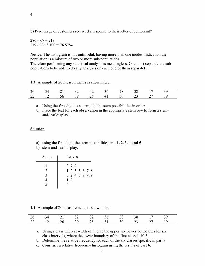
b) Percentage of customers received a response to their letter of complaint? 286 – 67 = 219 219 / 286 * 100 = 76.57% Notice: The histogram is not unimodal, having more than one modes, indication the population is a mixture of two or more sub-populations. Therefore performing any statistical analysis is meaningless. One must separate the sub-populations to be able to do any analyses on each one of them separately. 1.3: A sample of 20 measurements is shown here: 26 34 21 32 42 36 28 38 17 39 22 12 56 39 25 41 30 23 27 19
a. Using the first digit as a stem, list the stem possibilities in order. b. Place the leaf for each observation in the appropriate stem row to form a stem-
and-leaf display. Solution
a) using the first digit, the stem possibilities are: 1, 2, 3, 4 and 5 b) stem-and-leaf display:
Stems Leaves 1 2, 7, 9 2 1, 2, 3, 5, 6, 7, 8 3 0, 2, 4, 6, 8, 9, 9 4 1, 2 5 6
1.4: A sample of 20 measurements is shown here: 26 34 21 32 32 36 28 38 17 39 22 12 26 39 25 31 30 23 27 19
a. Using a class interval width of 5, give the upper and lower boundaries for six class intervals, where the lower boundary of the first class is 10.5.
b. Determine the relative frequency for each of the six classes specific in part a. c. Construct a relative frequency histogram using the results of part b.

5
5
Solution A sample of 20 measurements is shown here:
26 34 21 32 32 36 28 38 17 39 22 12 26 39 25 31 30 23 27 19
Class Class Interval Class Frequency Class Relative Frequency
1 10.5 – 15.5 1 .05 2 15.5 – 20.5 2 .1 3 20.5 – 25.5 4 .2 4 25.5 – 30.5 5 .25 5 30.5 – 35.5 4 .2 6 35.5 – 40.5 4 .2
Total 20 1.00
1.5: Suppose a data set contains the observations 3, 8, 4, 5, 3, 4, 6. Find: a. ∑x b. ∑x² c. ∑ (x-5) ² d. ∑ (x-2) ² e. (∑x) ² Solution a.
b.

6
6
c.
d.
e. 1.6: Find the mean and the median for the following sample of n = 6 measurements: 7, 3, 4, 1, 5, 6 Solution
1.7: Find the range, variance, and standard deviation for the following data set:
3 9 0 7 4 Use the shortcut procedure to calculate s². Solution Set: 3, 9, 0, 7, 4 Range = 9 – 0 = 9 Variance = s2 = [∑x2 - (∑x)2 /n] / n – 1 = ∑x2 - n(xbar)2 / n – 1 = [155 – 4.6] / 4 = 37.6 Standard Deviation = square root [∑(x – xbar)2 / n – 1] = sr [5.76 + 19.36 + 21.16 + 5.76 + 0.36] / 4 = sr(52.4 / 4) = sr(13.1) = 3.62 1.8: Compute z scores for each of the following situations. Then determine which x values lies the greatest distance above the mean; the greatest distance below the mean. a. x = 77, x = 58, s = 8 b. x = 8.8, x = 11, s = 2
7
7
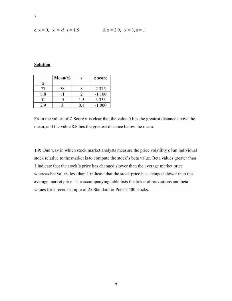
c. x = 0, x = -5, s = 1.5 d. x = 2.9, x = 3, s = .1
Solution
x
Mean(x) s z score
77 58 8 2.375 8.8 11 2 -1.100 0 -5 1.5 3.333
2.9 3 0.1 -1.000
From the values of Z Score it is clear that the value 0 lies the greatest distance above the
mean, and the value 8.8 lies the greatest distance below the mean.
1.9: One way in which stock market analysts measure the price volatility of an individual
stock relative to the market is to compute the stock’s beta value. Beta values greater than
1 indicate that the stock’s price has changed slower than the average market price
whereas bet values less than 1 indicate that the stock price has changed slower than the
average market price. The accompanying table lists the ticker abbreviations and beta
values for a recent sample of 25 Standard & Poor’s 500 stocks.
8
8
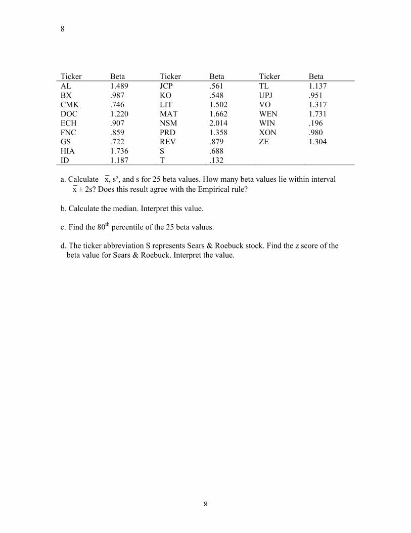
Ticker Beta Ticker Beta Ticker Beta AL 1.489 JCP .561 TL 1.137 BX .987 KO .548 UPJ .951 CMK .746 LIT 1.502 VO 1.317 DOC 1.220 MAT 1.662 WEN 1.731 ECH .907 NSM 2.014 WIN .196 FNC .859 PRD 1.358 XON .980 GS .722 REV .879 ZE 1.304 HIA 1.736 S .688 ID 1.187 T .132 a. Calculate x, s², and s for 25 beta values. How many beta values lie within interval x ± 2s? Does this result agree with the Empirical rule? b. Calculate the median. Interpret this value. c. Find the 80th percentile of the 25 beta values. d. The ticker abbreviation S represents Sears & Roebuck stock. Find the z score of the
beta value for Sears & Roebuck. Interpret the value.

9
9
Solution
Ticker Beta (x) x2 AL 1.489 2.217 BX 0.987 0.974 CMK 0.746 0.557 DOC 1.220 1.488 ECH 0.907 0.823 FNC 0.859 0.738 GS 0.722 0.521 HIA 1.736 3.014 ID 1.187 1.409 JCP 0.561 0.315 KO 0.548 0.300 LIT 1.502 2.256 MAT 1.662 2.762 NSM 2.014 4.056 PRD 1.358 1.844 REV 0.879 0.773 S 0.688 0.473 T 0.132 0.017 TL 1.137 1.293 UPJ 0.951 0.904 VO 1.317 1.734 WEN 1.731 2.996 WIN 0.196 0.038 XON 0.980 0.960 ZE 1.304 1.700 Total 26.813 34.165 a. ∑x =26.813
∑x2 =26.813 (∑x)2 =718.94 _ Mean xbar = 1.073 Variance, s2 = 0.225313 Standard deviation, s = 0.474671 Range : xbar - 2s = 0.123178, and xbar + 2s = 2.021862 All 25 values lies between these ranges. The Empirical rule states that close to 95% of observations will lie in this range for symmetric distributions, it also states that the percentage will be near 100% for highly skewed distributions. In this case because all 25 values lie in this range we can say that the values are symmetric and highly skewed.

10
10
b. Sorting the 25 numbers in ascending order we can see that the 13th number. 0.987, is the median. This means that of the remaining 24 numbers, 50%, or 12 numbers are smaller than this number and the other 12 numbers are greater than the mean.
0.132 0.196 0.548 0.561 0.688 0.722 0.746 0.859 0.879 0.907 0.951 0.980 0.987 1.137 1.187 1.220 1.304 1.317 1.358 1.489 1.502 1.662 1.731 1.736 2.014

11
11
c.
The 80th percentile = 80 x (25 + 1)/100
= 21
Therefore the 21st number, 1.502, is in the 80th percentile.
d.
Z Score of S = (x - xbar)/s
= (0.688 - 1.073)/ 0.474671
= -0.81008
The negative sign in the z score means that the observation lies to the left of the mean, because the absolute value. More Detailed Solution: One way in which stock market analysts measure the price volatility of an individual stock relative to the market is to compute the stock’s beta value. Beta values greater than 1 indicates that the stock’s price has changed faster than the average market price, whereas beta values less than 1 indicate that the stock’s price changed slower than the average market price. The accompanying table lists the ticker abbreviations and beta values for a recent sample of 25 Standard & Poor’s: http://www2.standardandpoors.com/servlet/Satellite?pagename=sp/Page/HomePg&r=1&l=EN 500 stocks.
12
12
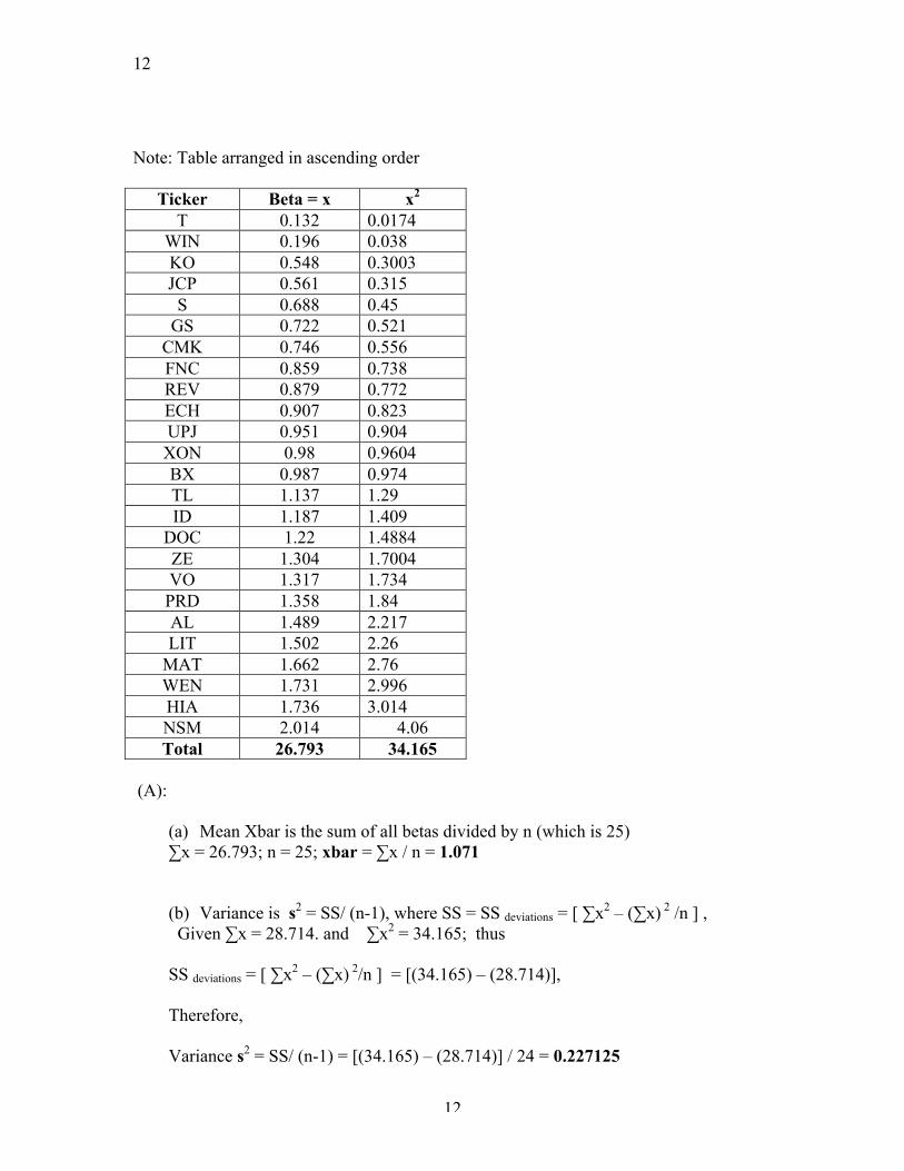
Note: Table arranged in ascending order
Ticker Beta = x x2 T 0.132 0.0174
WIN 0.196 0.038 KO 0.548 0.3003 JCP 0.561 0.315
S 0.688 0.45 GS 0.722 0.521
CMK 0.746 0.556 FNC 0.859 0.738 REV 0.879 0.772 ECH 0.907 0.823 UPJ 0.951 0.904 XON 0.98 0.9604 BX 0.987 0.974 TL 1.137 1.29 ID 1.187 1.409
DOC 1.22 1.4884 ZE 1.304 1.7004 VO 1.317 1.734
PRD 1.358 1.84 AL 1.489 2.217 LIT 1.502 2.26
MAT 1.662 2.76 WEN 1.731 2.996 HIA 1.736 3.014 NSM 2.014 4.06 Total 26.793 34.165
(A):
(a) Mean Xbar is the sum of all betas divided by n (which is 25) ∑x = 26.793; n = 25; xbar = ∑x / n = 1.071
(b) Variance is s2 = SS/ (n-1), where SS = SS deviations = [ ∑x2 – (∑x) 2 /n ] , Given ∑x = 28.714. and ∑x2 = 34.165; thus SS deviations = [ ∑x2 – (∑x) 2/n ] = [(34.165) – (28.714)], Therefore, Variance s2 = SS/ (n-1) = [(34.165) – (28.714)] / 24 = 0.227125
13
13
(c) Standard Deviation is s = √s2 = √ (0.227125) = 0.4765
(d) xbar + 2 s = 2.024 ; xbar – 2s = 0.118;
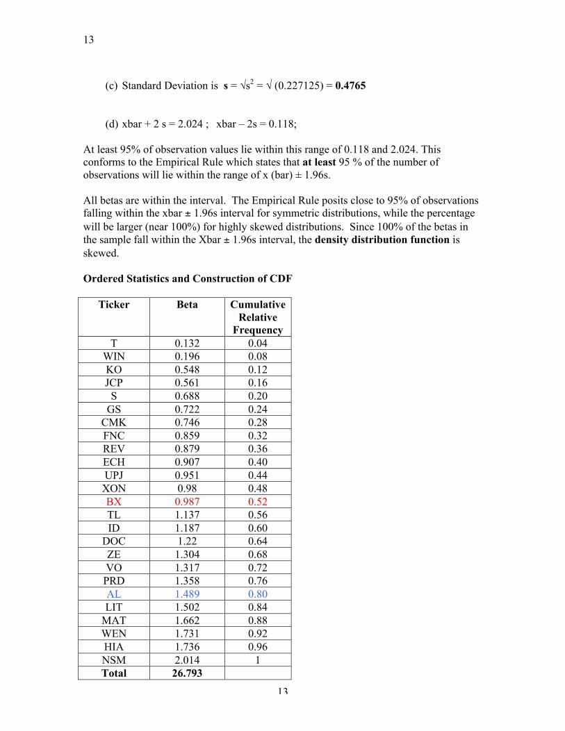
At least 95% of observation values lie within this range of 0.118 and 2.024. This conforms to the Empirical Rule which states that at least 95 % of the number of observations will lie within the range of x (bar) ± 1.96s. All betas are within the interval. The Empirical Rule posits close to 95% of observations falling within the xbar ± 1.96s interval for symmetric distributions, while the percentage will be larger (near 100%) for highly skewed distributions. Since 100% of the betas in the sample fall within the Xbar ± 1.96s interval, the density distribution function is skewed. Ordered Statistics and Construction of CDF
Ticker Beta Cumulative Relative
Frequency T 0.132 0.04
WIN 0.196 0.08 KO 0.548 0.12 JCP 0.561 0.16
S 0.688 0.20 GS 0.722 0.24
CMK 0.746 0.28 FNC 0.859 0.32 REV 0.879 0.36 ECH 0.907 0.40 UPJ 0.951 0.44 XON 0.98 0.48 BX 0.987 0.52 TL 1.137 0.56 ID 1.187 0.60
DOC 1.22 0.64 ZE 1.304 0.68 VO 1.317 0.72
PRD 1.358 0.76 AL 1.489 0.80 LIT 1.502 0.84
MAT 1.662 0.88 WEN 1.731 0.92 HIA 1.736 0.96 NSM 2.014 1 Total 26.793

14
14
(B): Median is the 13th number as there are odd numbers of observations. Hence median is 0.987. Notice that, the median value is .987 and the mean is 1.073. The data set is skewed to the right (C): pth percentile = p(n+1) / 100; Hence the 80th percentile = 80(25+1) / 100 = 20.8 which is approximated to the 21st number which is 1.502. (D): z = {x – xbar) / s = (0.668 – 1.071) / 0.4765 = - 0.8458 A negative z – score indicates that the observation lies to the left of the mean. Because the data set is skewed, the Z score needs to be less than 1 for this value not to be an outlier. Therefore the beta of Sears & Roebuck is most likely not an outlier.

15
15

16
16
Notice: The histogram is not unimodal, having more than one modes, indication the population is a mixture of two or more sub-populations. Therefore performing any statistical analysis is meaningless. One must separate the sub-populations to be able to do any analyses on each one of them separately. - Other applications of Z-Scores

17
17
2. Probability Concepts and Applications 2.1: In New York City, the leading cause of death on the job is not construction accidents, machinery malfunctions, or car crashes – it is homicide! A federal Bureau of labor Statistics study revealed that of 177 New York City workers who died of injuries sustained on the job last year,122 were homicide victims. Use this information to estimate the probability that an on-the-job death of a New York City worker is the result of a homicide. Solution The probability that an on-the-job death of a New York City worker is the result of a homicide is:
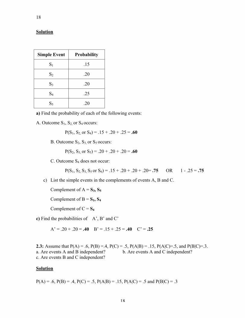
2.2: An experiment has 5 possible outcomes (simple events) with the following probabilities:
Simple Event Probability
S1 .15 S2 .20 S3 .20 S4 .25 S5 .20
a. Find the probability of each of the following events:
A: Outcome S1, S2, or S4 occurs. B: Outcome S2, S3, or S5 occurs. C: Outcome S4 does not occur.
b. List the simple events in the complements of events A, B and C. c. Find the probabilities of Ā, B and C.
18
18
Solution
Simple Event Probability
S1 .15
S2 .20
S3 .20
S4 .25
S5 .20
a) Find the probability of each of the following events:
A. Outcome S1, S2, or S4 occurs:
P(S1, S2, or S4) = .15 + .20 + .25 = .60
B. Outcome S2, S3, or S5 occurs:
P(S2, S3, or S5) = .20 + .20 + .20 = .60
C. Outcome S4 does not occur:
P(S1, S2, S3, S5 or S6) = .15 + .20 + .20 + .20= .75 OR 1 - .25 = .75
c) List the simple events in the complements of events A, B and C.
Complement of A = S3, S5
Complement of B = S1, S4
Complement of C = S4
c) Find the probabilities of A’, B’ and C’
A’ = .20 + .20 = .40 B’ = .15 + .25 = .40 C’ = .25
2.3: Assume that P(A) = .6, P(B) =.4, P(C) = .5, P(A|B) = .15, P(A|C)=.5, and P(B|C)=.3. a. Are events A and B independent? b. Are events A and C independent? c. Are events B and C independent? Solution P(A) = .6, P(B) = .4, P(C) = .5, P(A|B) = .15, P(A|C) = .5 and P(B|C) = .3

19
19
2.3: According to a report from the Newspaper Advertising Bureau, 40% of all primary car maintainers are women. Consequently, advertisements for car care products, traditionally geared toward men, are now being aimed at women also. Consider the population consisting of all primary car maintainers.
a. What is the probability that a primary car maintainer, selected from the population, is a woman? A man?
b. What is the probability that both primary car maintainers in a sample of two selected from the population are women?
Solution
P(woman) = .40 P(man) = .60
b) What is the probability that both car maintainers in a sample of two selected from the population are women?
P(W) = .40 * .40 = .16
2.4: For two events A and B, P(A) = .5, P(B) = .6, and P(both A and B occur) = .4. Find the probability that either A or B or both occur. Solution
a) Are events A and B independent?
P(A) = .6, P(B) = .4 and P(A|B) = .15. They are not independent, because P(A|B) ≠ P(A)
b) Are events A and C independent?
P(A) = .6, P(C) = .5 and P(A|C) = .5. They are not independent, because P(A|C) ≠ P(A)
c) Are events B and C independent?
P(B) = .4, P(C) = .5 and P(B|C) = .3. They are not independent, because P(B|C) ≠ P(B)
2.5: P(A or B or both) = P(A) + P(B) – P(A and B) = .5 + .6 - .4 = .7 The merging process from an acceleration lane to the through lane of a freeway constitutes an important aspect of traffic operation at interchanges. From a study of parallel and tapered interchange ramps in Israel, the table provides information on traffic

20
20
lags (where a lag is defined as an interval of time between arrivals of major streams of vehicles) accepted and rejected by drivers in the merging lane.
Type of Interchange
Lane
Traffic Condition
On Freewway
Number of Merging Drivers Accepting the First Available
Lag
Number of Merging Drivers Rejecting the First Available
Lag Tapered Heavy Traffic
Little Traffic 16 67
115 121
Parallel Heavy Traffic Little Traffic
40 144
139 331
a. What is the probability that a driver in a tapered merging lane with heavy traffic
will accept the first available lag? b. What is the probability that a driver in a parallel merging lane with heavy traffic
will reject the first available lag? c. Given that a driver accepts the first available lag in little traffic, what is the
probability that the driver is in a parallel merging lane?
a)
b)
c)

21
21
3. Probability Distributions with Applications
3.1: A discrete random variable can assume 5 possible values, as listed in the accompanying probability distribution. X 1 2 4 5 8 P (x) .20 .25 - .30 .10
a. Find the missing value for p(4). b. Find the probability that x = 2 or x = 4.
Solution a) P (4) = 1 – (.20 + .25 + .30 + .10) = .15
b) x = 2 or x = 4?
P(2) = .25 P(4) = .15
P(x=2 or x=4) = P(2) + P(4) = .25 + .15 = .40
c) P(x≤ 4) = P(1) + P(2) + P(4) = .20 + .25 + .15 = .60
3.2: Find µ and σ for the probability distribution in exercise 3.1 Solution
3.3: A coin is tossed 10 times and the number of heads is recorded. To a reasonable degree of approximation, is this a binomial experiment? Check to determine whether each of the five conditions required for a binomial experiment is satisfied. Solution The example is a binomial experiment, because it meets all the required conditions for a binomial experiment.
1. A sample of n experiment units is selected from a population.
Yes, n is 10 in this example.

22
22
2. Each experimental unit possesses one of two characteristics, success or failure.
Each flip of the coin is one experimental unit. Heads can represent “success”, while the tail represents “failure”.
3. The probability that a single experimental unit possesses the “success” characteristic is equal to π. This probability is the same for all experimental units.
Each flip of coin has the same probability of having a “success” or a “failure”.
4. The outcome for any one experimental unit is independent of the outcome for any other experimental unit.
Each flip of coin is independent of the other.
5. The random variable x counts the number of “successes” in n trails.
This is also true for tossing of coins.
3.4: In a study, Consumer Reports found widespread contamination and mislabeling of seafood in the markets in New York City and Chicago. The study revealed one alarming statistic: 40% of the swordfish pieces available for sale had a high level of mercury above the Food and Drug administration (FDA) maximum amount. In a random sample of the three swordfish pieces, find the probability that:
a. All three swordfish pieces have a mercury level above FDA maximum. b. Exactly one swordfish piece has a mercury level above the FDA maximum. c. At most one swordfish piece has a mercury level above the FDA maximum.
Solution
a)
b)
c) P(x=0 or x=1) = P(x=0) + P(x=1)

23
23
P(x=0 or x=1) = .216+ .432 = .648 3.5: Occupational Outlook Quarterly recently reported that 1% of all the drywall installers employed in the construction industry are women. In a random sample of 10 drywall installers find the probability that at most one is a woman. Solution A binomial distribution with n = 10, and π = 0.01 P(at most one woman) = P (x less than OR equal to 1) From the Binomial, with n = 10 and π = 0.01, we find P(at most one woman) = 0.9957 3.6: According to the American Hotel and Motel Association, women are expected to account for half of all business travelers by the last year. To attract these women business travelers, hotels are providing more amenities that women particularly like, such as shampoo, conditioner, and body lotion. A survey of American hotels found that 86% offer shampoo in their guest rooms. Consider random sample of five hotels, and let x be the number that provide shampoo as a guest room amenity.
a. To a reasonable degree of approximation, is this a binomial experiment? b. What is the “success” in the context of this experiment? c. What is the value of π ? d. Find the probability that x = 4. e. Find the probability that x ≥ 4.
Solution
A). Yes, because: 1. n=5 2. Two outcomes 3. π = 86% 4. outcome independent 5. random variable counts number of successes Therefore qualifies as a binomial experiment. B.) a hotel that has shampoo C.) pie = 86% D.) P(x = 4) = 0. 3829

24
24
E.) P(x > 4) = P (4) + P (5) = 0.3829 + 0.4704 = 0.8533 3.7: Find the area under the standard normal curve: a. Between z = 0 and z = 1.96 b. Between z = -1.96 and z = 0 c. Between z = -1.96 and z = 1.96 d. For values of z larger than .55 f. For values of z less than –1.24. Show the values of z and corresponding area of interest on a sketch of the normal curve for each part of the exercise. Solution Using the left margin column together with the top margin row of Normal Table:
A.) .4750 B.) .4750 C.) 0.4750 + 0.4750 = .9500 D.) 0.5 - 0.2088 = 0.2912 E.) 0.5 - 0.3925 = 0.1075
3.8: Find the value of z (to 2 decimal places) that cuts off an area in the upper tail of the standard normal curve equal to: a. 0.25 b. 0.05 c. 0.005 d. 0.01 e. 0.10 Show the area and corresponding value of z on a sketch of the normal curve for each part of the exercise. Solution Looking in the body of Normal Table
A.) 1.96 B.) 1.64 or 1.65. Better to say 1.645 C.) 2.57 or 2.58. Better to say 2.575 D.) 2.33 E.) 1.28
3.9: Find the approximate value for z0 such that the probability that z is larger than z0 is:

25
25
a. P = .10 b. P= .15 c. P = .20 d. P = .25 Locate z0 and the corresponding probability P on a sketch of the normal curve for each part of the exercise. Solution P-value is the area to the tail, therefore using Normal Table:
A.) 1.28 B.) 1.04 C.) .84 D.) .67
3.10: Researchers have developed sophisticated intrusion-detection algorithms to protect eth security of computer-based systems. These algorithms use principles of statistics to identify unusual or expected data, i.e., “intruders.” One popular intrusion-detection system assumes the data being monitored are normally distributed. As an example, the researcher considered system data with a mean of .27, a standard deviation of 1.473, and an intrusion-detection algorithm that assumes normal data.
a. Find the probability that a data value observed by the system will fall between - .5 and .5.
b. Find the probability that a data value observed bye the system exceeds 3.5. c. Comment on whether a data value of 4 observed by the system should be
considered an “intruder”. Solution After Z-transformation of the random variable X, you use Normal Table:
A.) x between -0.5, and 0.5 is equivalent to z between -.53 and 0.16. Using From Normal Table, we have 0.2019 + 0.0636 = 0.2655
B.) x greater than 3.5 is equivalent to z greater than 2.19. Using From Normal Table, we have 0.5 - 0.4857 = 0.0143
C.) Based on Part B. an observed value of 4 is very unlikely, therefore, it is an “intruder”
3.11: The Journal of Information Systems study of intrusion-detection systems. According to the study many intrusion-detection systems assume that data being monitored are normally distributed when such data are clearly non-normal. Consequently, the intrusion-detection system may lead to inappropriate conclusions. Te researcher considered the following data on input-output (I/O) units utilized by a sample of 44 users of a system.

26
26
15 5 2 17 4 3 1 1 0 0 0 0 0 0 0 20 9 0 0 0 1 6 1 3 1 0 6 0 0 0 0 1 14 0 7 0 2 9 4 0 0 0 9 10 Based on the accompanying MINITAB printouts, assess whether the data are normally distributed. Stem-and-leaf of I/O N = 44 Leaf Unit = 1.0
(26) 0 00000000000000000000111111 18 0 2233 14 0 445 11 0 667 8 0 999 5 1 0 4 1 4 1 45 2 1 7 1 1 1 2 0
I/O N
44 MEAN 3.432
MEDIAN 1.000
TRMEAN 2.850
STDEV 5.160
SEMEAN 0.778
I/0 MIN
0.000 MAX 20.000
Q1 0.000
Q3 5.750
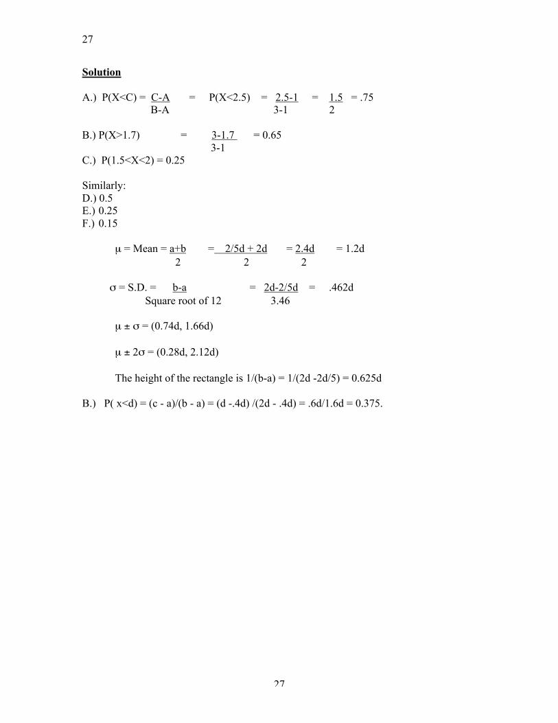
Solution The stem and leaf plot does not show a symmetric shape 3.12: Suppose x is a uniform random variable over the interval 1≤ x ≤ 3. Find the following probabilities: a. P (x <2.5) b. P ( x > 1.7) c. P (1.5 < x < 2) d. P ( x < 2) e. p(1.1 ≤ x ≤ 1.6) f. P(x ≤ 1.3)
27
27
Solution A.) P(X<C) = C-A = P(X<2.5) = 2.5-1 = 1.5 = .75 B-A 3-1 2 B.) P(X>1.7) = 3-1.7 = 0.65 3-1 C.) P(1.5<X<2) = 0.25 Similarly: D.) 0.5 E.) 0.25 F.) 0.15 µ = Mean = a+b = 2/5d + 2d = 2.4d = 1.2d 2 2 2 σ = S.D. = b-a = 2d-2/5d = .462d Square root of 12 3.46 µ ± σ = (0.74d, 1.66d) µ ± 2σ = (0.28d, 2.12d) The height of the rectangle is 1/(b-a) = 1/(2d -2d/5) = 0.625d B.) P( x<d) = (c - a)/(b - a) = (d -.4d) /(2d - .4d) = .6d/1.6d = 0.375.

28
28
4. Estimation with Confidence
4.1: Suppose a random sample of n measurements is selected from a population with mean µ = 60 and variance σ ² = 100. For each of the following values of n, give the mean and standard deviation of the sampling distribution of the sample mean, x: a. n = 10 b. n = 25 c. n = 50 d. n = 75 e. n = 100 f. n = 500 g. n = 1,000 Solution µ = 60,
n Mean Standard Deviation
10 60 3.1623
25 60 2
50 60 1.414
75 60 1.555
100 60 1
500 60 0.447
1000 60 0.316
For ex a)
4.2: The National Institute for Occupational Safety and Health (NIOSH) recently completed a study to evaluate the level of exposure of workers to the chemical dioxin, 2, 3, 7, 8-TCDD. The distribution of TCDD levels in parts per trillion (ppt) in production workers at a Newark, New Jersey, chemical plant had a mean of 293 ppt and a standard deviation of 847 ppt. A graph of the distribution is shown here.
500 1000 1500 2000
.20
.10

29
29
In a random sample of n = 50 workers selected at eth New Jersey plant, let x represent the sample TDCC level.
a. Find the mean and standard deviation of the sampling distribution of x. b. Draw a sketch of the sampling distribution of x. Locate the mean on the graph. c. Find the probability that x exceeds 550 ppt.
Solution n = 50, µ = 293,
a) µ = 293,
b)
µ = 293
c) z-score =
P(x exceeds 550ppt) = 0.5 – 0.4842 = 0.0158 = 1.58% 4.3: The manufacturer of a new instant-picture camera claims that its product had “the world’s fastest-developing color film by far.” Extensive laboratory testing has shown that the relative frequency distribution for the time it takes the new instant camera to begin to reveal the image after shooting has a mean of 9.8 seconds and a standard deviation of .55 second. Suppose 50 of these cameras are randomly selected from the production line and tested. The time until the image is revealed, x, is recorded fro each.
a. Describe the sampling distribution of x, the mean time it takes the sample of 50 cameras begin to reveal the image.
b. Find the probability that the mean time until the image is first revealed for the 50 sampled cameras is greater than 9.70 seconds.
c. If the mean and standard deviation of the population relative frequency distribution for the times until the cameras begin to reveal the image are correct, would you expect to observe a value of x less than 9.55 seconds? Explain.

30
30
d. Refer to part a. Describe the changes in the sampling distribution of x if the sample size were decreased from n = 50 to n = 20.
e. Repeat part d if the sample size were increased from n = 50 to n = 100.
Solution n = 50, µ = 9.8, a) It is approximately normal. The standard deviation of the sampling distribution would be smaller than that of the population.
b)
z-score = (9.7 – 9.8) / 0.07778 = -1.286
P(x>9.70) = 0.5 + 0.4015 = 0.9015
c) z-score = (9.55 – 9.8) / 0.07778 = -3.21
P(x<9.55) = 0.00065. The probability is almost zero. I would not expect to observe a value less than 9.55 seconds.
d) n=20 , with a smaller sample size, the sampling distribution would become more spread out and start to deviate from normal
e) n=100, with a larger sample size, the sampling distribution would become less spread out and would be closer to normal distribution.
4.4: A random sample of size n is selected from an unknown population with mean µ and standard deviation σ. Calculate a 95% confidence interval for µ for each of eth following situations: a. n = 35, x = 26, s² = 228.2 b. n = 70,x = 24.1, s² = 198.4 c. n = 105,x = 24.2, s² = 216.9 Solution 95% confidence interval
n xbar s2 min max
35 26 228.2 21.00 31.00
70 24.1 198.4 20.80 27.40
105 24.2 216.9 21.38 27.02

31
31
4.5: According to a study in Administrative Science Quarterly, the salary gap between Chief executive officer (CEO) of a firm and a Vice President (VP) is often very large, and the gap appears to increase the more VPs a firm employs. Based on data collected for a sample of 105 U.S. firms drawn from Business Week’s executive Compensation Scoreboard, the mean and standard deviation of the number of VPs employed by a firm are x = 19.4 and s = 10.1. Use this information to estimate the true mean number of VPs at U.S. firms with a 90% confidence interval. Interpret the result. Solution
n xbar s min max
105 19.4 10.1 17.78 21.02
We are 90% confident that the mean number of VPs for all US firms will fall between 18 and 21. 4.6: Give two reasons why the CLT-based interval estimation procedure for the population mean may not be applicable when the sample size is small. Solution When the sample size is small, the central limit theorem does not apply. The standard deviation of the sample does not approximate the true standard deviation of the population. 4.7: The following data represent a random sample of five measurements from a normally distributed population:
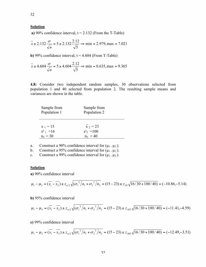
7 4 2 5 7 a. Find a 90% confidence interval for µ. B. Find a 99% confidence interval for µ.
32
32
Solution a) 90% confidence interval, t = 2.132 (From the T-Table)
b) 99% confidence interval, t = 4.604 (From T-Table)
4.8: Consider two independent random samples, 30 observations selected from population 1 and 40 selected from population 2. The resulting sample means and variances are shown in the table.
Sample from Population 1
Sample from Population 2
x 1 = 15
x 2 = 23
s² 1 =16 s²2 =100 n1 = 30 n2 = 40
a. Construct a 90% confidence interval for (µ1 - µ2 ). b. Construct a 95% confidence interval for (µ1 - µ2 ). c. Construct a 99% confidence interval for (µ1 - µ2 ). Solution a) 90% confidence interval
b) 95% confidence interval
c) 99% confidence interval

33
33
4.9: A Harris Corporation/University of Florida study was undertaken to determine whether a manufacturing process performed at a remote location can be established locally. Test devices (pilots) were set up at both the old and new locations, and voltage readings on the process were obtained. A “good process” was considered to be one with voltage readings of at least 9.2 volts (with larger readings being better than small readings).The table contains voltage readings for 30 production runs at each location. Descriptive statistics for both sample data sets are provided in the SAS printout below. We wish to determine whether a manufacturing process performed at a remote location can be established locally, test devices (pilots) were set up at both the old and new locations and voltage readings on 30 production runs at each location were obtained. The data are reproduced in the table. Descriptive statistics are displayed in the accompanying SAS printout. [Note: larger voltage readings are better tan smaller voltage readings.]
Old Location New Location 9.98 10.12 9.84 9.19 10.01 8.82 10.26 10.05 10.15 9.63 8.82 8.65 10.05 9.80 10.02 10.10 9.43 8.51 10.29 10.15 9.80 9.70 10.03 9.14 10.03 10.00 9.73 10.09 9.85 9.75 8.05 9.87 10.01 9.60 9.27 8.78 10.55 9.55 9.98 10.05 8.83 9.35 10.26 9.95 8.72 10.12 9.39 9.54 9.97 9.70 8.80 9.49 9.48 9.36 9.87 8.72 9.84 9.37 9.64 8.68 Analysis Variable: Voltage
----------------------------------------LOCATION=OLD-------------------------------------------
N Obs N Minimum Maximum Mean Std Dev ------------------------------------------------------------------------------------------------------------ 30 30 8.0500000 10.5500000 9.8036667 0.5409155 ------------------------------------------------------------------------------------------------------------ -----------------------------------------LOCATION=NEW-----------------------------------------
N Obs N Minimum Maximum Mean Std Dev ------------------------------------------------------------------------------------------------------ 30 30 8.5100000 10.1200000 9.4223333 0.4788757
34
34
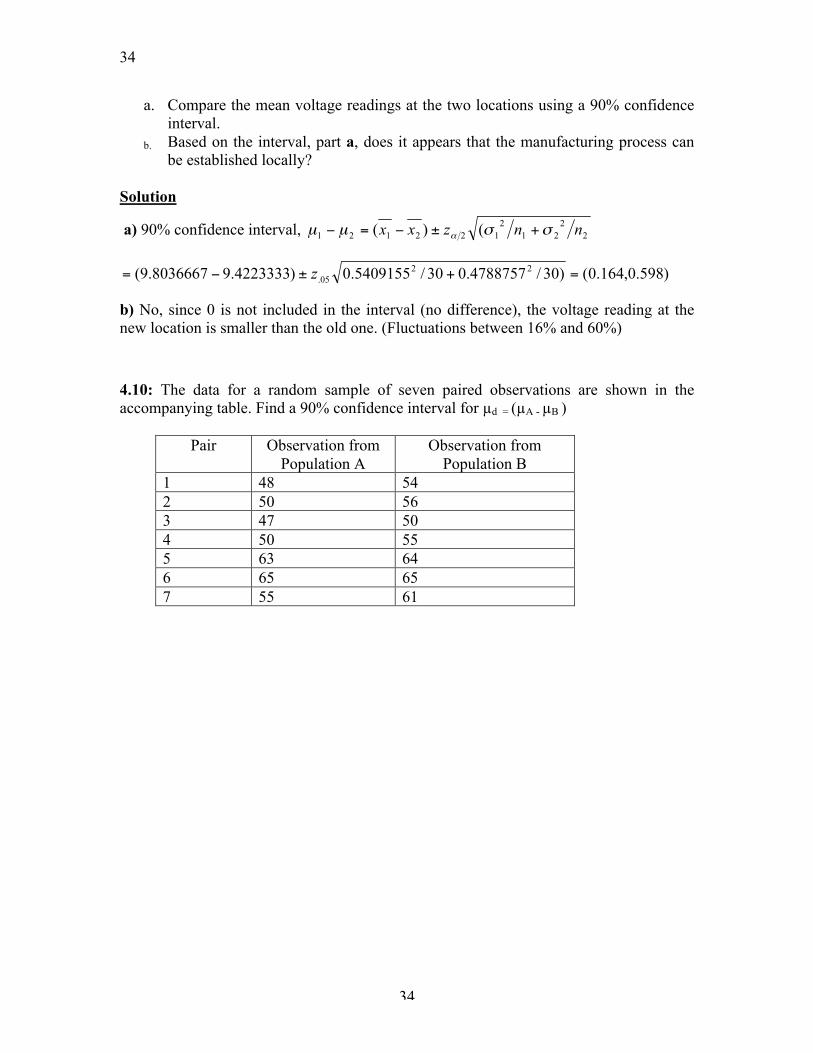
a. Compare the mean voltage readings at the two locations using a 90% confidence interval.
b. Based on the interval, part a, does it appears that the manufacturing process can be established locally?
Solution
a) 90% confidence interval,
b) No, since 0 is not included in the interval (no difference), the voltage reading at the new location is smaller than the old one. (Fluctuations between 16% and 60%) 4.10: The data for a random sample of seven paired observations are shown in the accompanying table. Find a 90% confidence interval for µd = (µA - µB )
Pair Observation from Population A
Observation from Population B
1 48 54 2 50 56 3 47 50 4 50 55 5 63 64 6 65 65 7 55 61

35
35
Solution
Pair Observation from A Observation from B Difference
1 48 54 -6
2 50 56 -6
3 47 50 -3
4 50 55 -5
5 63 64 -1
6 65 65 0
7 55 61 -6
(-6)+(-6)+(-3)+(-5)+(-1)+(0)+(-6) = - 27 / 7 = -3.857 =dbar
4.11: Given the following values x, s, n, calculate a 90% confidence interval for σ² a. x = 21, s = 2.5, n = 50 b. x = 1.3, s = .02, n = 15 c. x = 167, s = 31.6, n = 22 d. x = 9.4, s = 1.5, n = 5 Solution
xbar s n min max
21 2.5 50 4.536 8.809
1.3 .02 15 0.00023 0.00085
167 31.6 22 641.856 1809.095
9.4 1.5 5 0.946 12.663
= (50-1)2.52/67.5048 ≤ σ2 ≤(50-1)2.52/34.7647 (From Chi-Squired Table)
= (4.536, 8.809)

36
36
5. Hypothesis Testing with Applications 5.1: A study reported whether the mean performance appraisal of “leavers” at a large national oil company is less than the mean performance appraisal of “stayers.” Formulate the appropriate null and alternative hypotheses for the study.
Solution
The researcher is interested to know if the mean performance appraisal of "leavers" is
less than the mean performance appraisal of the "stayers".
If µ1 is the mean performance appraisal of "leavers", and µ1, the mean performance
appraisal of the "stayers" then:
Ha: (µ1 - µ2) < 0
H0: (µ1 - µ2) = 0
One tailed test is performed because the researchers are interested only if the mean
performance appraisal of "leavers" if less than the mean performance appraisal of
"stayers".
5.2: Refer to exercise the above problem. Interpret the Type I and Type II errors in the context of the problem. Using the hypothesis from above;
Ha: (µ1 - µ2) < 0
H0: (µ1 - µ2) = 0
Solution
A Type I error is that of incorrectly rejecting the null hypothesis. This would occur if we
conclude that the mean performance appraisal of "leavers" is less than the mean
performance appraisal of "stayers", when, in fact, when they are equal.
The consequence of making such an error is that we are loosing more good employees
thinking that they are under performers.
A Type II error is that of incorrectly accepting the null hypothesis. This would occur if
we conclude that the mean performance appraisal of "leavers" is equal to the mean
performance appraisal of "stayers", when, in fact, when they are less.

37
37
The consequence of making such an error is that we are retaining more under performing
employees thinking that they are good performers.
5.3: Suppose it is desired to test H0 : µ = 65. Specify the form of the rejection region for each of the following (assume tat the sample size will be sufficient to guarantee the approximate normality of the sampling distribution of x): a. Ha : µ ≠ 65, α = .02 b. Ha : µ > 65, α = .05 c. Ha : µ < 5, α = .01 d. Ha : µ < 65, α = .10
Solution
a. Ha : µ ≠ 65, α =.02
Because this is a two sided alternate hypothesis, Zα/2 =Z.01 = 2.326
Chance of observing a sample mean Xbar less than 2.33 standard deviations below 65
or more than 2.326 standard deviations above 65, when H0 is true, is only .02, i.e.,
probability of type 1 error is .02
b. Ha : µ > 65, α =.05
Because this is a one sided alternate hypothesis, Zα/ =Z.05 = 1.645
Chance of observing a sample mean Xbar more than 1.645 standard deviations above
65, when H0 is true, is only .05, i.e., probability of type 1 error is .05
c. Ha : µ < 65, α =.01
Because this is a one sided alternate hypothesis, Zα/ =Z.01 = -2.326
Chance of observing a sample mean Xbar more than 2.326 standard deviations below
65, when H0 is true, is only .01, i.e., probability of type 1 error is .01
d. Ha : µ < 65, α =.10
Because this is a one sided alternate hypothesis, Zα/ =Z.10 = -1.282
Chance of observing a sample mean Xbar more than 1.282 standard deviations below
65, when H0 is true, is only .10, i.e., probability of type 1 error is .10
38
38
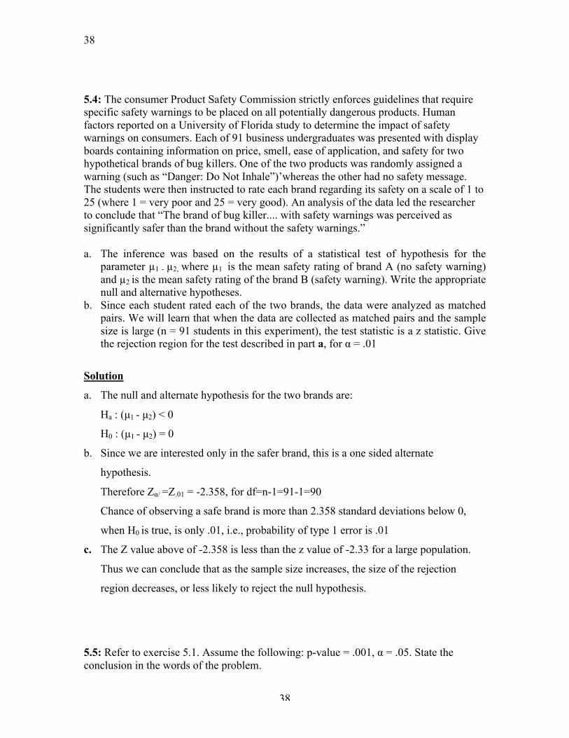
5.4: The consumer Product Safety Commission strictly enforces guidelines that require specific safety warnings to be placed on all potentially dangerous products. Human factors reported on a University of Florida study to determine the impact of safety warnings on consumers. Each of 91 business undergraduates was presented with display boards containing information on price, smell, ease of application, and safety for two hypothetical brands of bug killers. One of the two products was randomly assigned a warning (such as “Danger: Do Not Inhale”)’whereas the other had no safety message. The students were then instructed to rate each brand regarding its safety on a scale of 1 to 25 (where 1 = very poor and 25 = very good). An analysis of the data led the researcher to conclude that “The brand of bug killer.... with safety warnings was perceived as significantly safer than the brand without the safety warnings.” a. The inference was based on the results of a statistical test of hypothesis for the
parameter µ1 - µ2, where µ1 is the mean safety rating of brand A (no safety warning) and µ2 is the mean safety rating of the brand B (safety warning). Write the appropriate null and alternative hypotheses.
b. Since each student rated each of the two brands, the data were analyzed as matched pairs. We will learn that when the data are collected as matched pairs and the sample size is large (n = 91 students in this experiment), the test statistic is a z statistic. Give the rejection region for the test described in part a, for α = .01
Solution
a. The null and alternate hypothesis for the two brands are:
Ha : (µ1 - µ2) < 0
H0 : (µ1 - µ2) = 0
b. Since we are interested only in the safer brand, this is a one sided alternate
hypothesis.
Therefore Zα/ =Z.01 = -2.358, for df=n-1=91-1=90
Chance of observing a safe brand is more than 2.358 standard deviations below 0,
when H0 is true, is only .01, i.e., probability of type 1 error is .01
c. The Z value above of -2.358 is less than the z value of -2.33 for a large population.
Thus we can conclude that as the sample size increases, the size of the rejection
region decreases, or less likely to reject the null hypothesis.
5.5: Refer to exercise 5.1. Assume the following: p-value = .001, α = .05. State the conclusion in the words of the problem.

39
39
Solution
Since the p-value of .001 is less than .01, we would see very strong evidence against H0.
Also, because it is less than the maximum tolerable Type I error of α = .05, we will reject
the null hypothesis and conclude that the mean performance appraisal of "leavers" is less
than the mean performance appraisal of "stayers".
5.6: A random sample of n observations is selected from a population with unknown mean µ and variance σ². For each of the following situations, specify the test statistic and rejection region.
a. H0 : µ = 50, Ha : µ > 50, n = 36, x = 60, s² = 64, α = .05 b. H0 : µ = 140, Ha : µ ≠ 140, n = 40, x = 143.2, s = 9.4, α = .01 c. H0 : µ = 10, Ha : µ < 10, n = 50, x = 9.5, s = .35, α = .10
Solution
Since the sample size for all the three problems is greater than 30, we will use the Large-
sample Test statistic using the Z value.
a. H0 : µ = 50, Ha : µ > 50, n = 36, Xbar = 60, s2 = 64, α =.05
This is a one-tailed test, therefore using the significant level of α =.05, we will reject
the null
hypothesis for this one tailed test if Z > Z.05 = 1.645
Test statistic: z = (Xbar - µ0)/(s/√n) = (60 - 50)/( 8/√36) = 7.5
b. H0 : µ = 140, Ha : µ ≠ 140, n = 40, Xbar = 143.2 , s = 9.4, α =.01
This is a two-tailed test, therefore using the significant level of α =.01, we will reject
the null
hypothesis for this one tailed test if |Z| > Zα//2 (Zα//2 = Z.005 = 2.576)
Test statistic: z = (Xbar - µ0)/(s/√n) = (143.2 - 140)/(9.4/√40) = 2.1530
c. H0 : µ = 10, Ha : µ < 10, n = 50, Xbar = 9.5, s = .35, α =.10
This is a one-tailed test, therefore using the significant level of α =.10 we will reject
the null
hypothesis for this one tailed test if Z < -Z.10 = -1.282
Test statistic: z = (Xbar - µ0)/(s/√n) = (9.5 - 10)/( .35/√50) = -10.1015

40
40
5.7: Stocks on the National Association of Security Dealers (NASD) system were analyzed in Financial Analysts Journal. The annualized monthly returns for a sample of 13 large-firm NASD stocks were computed and are summarized as follows: x = 13.50%, s = 23.84%. Conduct a test hypothesis to determine whether the mean annualized monthly return for large-firm NASD stocks exceeds 10%. Use α = .05.
Solution
In this problem, the experimental units are the large-firm NASD stocks, and the variables
measured are the annualized monthly returns of 13 firms.
To determine whether the annualized monthly return for these stocks exceed 10%, we
will conduct a test of:
H0 : µ = 10 (no change in annualized monthly return)
Ha : µ > 10 (annualized monthly return has increased)
Since n is small we will treat this as a small sample and use the one-tailed test.
Using the significant level of α =.05 we will reject the null hypothesis for this one tailed
test if
t > t.05 = 1.782, df= (13-1) =12
Test statistic: t = (Xbar - µ0)/(s/√n) = (13.5 - 10)/ (23.84/√13) = 0.5293
Since the Z value does not fall within the rejection region, for α = .05, we will accept the
null hypothesis, and conclude that the annualized monthly return does not exceed 10%.
5.8: As a result of recent advances in educational telecommunications, many colleges and universities are utilizing instruction by interactive television for “distance” education. For example, each semester, Ball State University televises six graduate business courses to students at remote off-campus sites. To compare the performance of the off-campus MBA students at Ball State (who take the televised classes) to the on –campus MBA students (who have a “live” professor), a test devised by the assembly of Collegiate Schools of Business (AACSB) was administered to a sample of both groups of students. (The test included seven exams covering accounting, business strategy, finance, human resources, marketing, management information systems, and production and operations management.) The AACSB test scores (50 points maximum) are summarized in the table. Based on these results, the researchers report that “there was no significant difference between the two groups of students.” Mean Standard Deviation On-Campus Students 41.93 2.86

41
41
Off-Campus TV Students 44.56 1.42
Solution
a. The null and alternate hypothesis for the two groups are:
Ha : (µ1 - µ2) = 0 (no difference between groups)
H0 : (µ1 - µ2) ≠ 0 (the two groups differ)
This is a two-tailed test, and because the sample size is 50, the test is based on z
statistic.
Because the researcher was pretty confident about the outcome we will use a 99%
confidence
interval. i.e. (1- α = .99) or α =.01
Thus we will reject the null hypothesis if |Z| > Zα//2 (Zα//2 = Z.005 = 2.576)
Test statistic Z = (X1bar - X2bar)/ √(s12/n1 + s2
2/n2)
= (41.93 - 44.56)/ √(2.862/50 + 1.422/50) = -5.8240
Because the Z value falls within the rejection region, for α = .01, we will reject the null
hypothesis, and conclude that there is some significant difference between the two
groups.
b. If only 15 students are used we will have to use the small-sample test using the t
statistic, and
the formula where n1= n2 = n
Again because the researcher was pretty confident about the outcome we will use a
99%
confidence interval. i.e. (1- α = .99) or α =.01, and get the z value for df = 2(n-1) =
2(14) = 28
Thus we will reject the null hypothesis if |t| > tα//2 (tα//2 = t.005 = 2.763)
Test statistic t = (X1bar - X2bar)/ √1/n(s12
+ s22)
= (41.93 - 44.56)/ √1/15(2.862 + 1.422) = -3.1899
Because the Z value falls within the rejection region, for α = .01, we will reject the null hypothesis, and conclude that there is some significant difference between the two groups.

42
42
5.9: Consider the following summary statistics for a matched-pairs experiment: d = 10.5 Sd = 10
a. Suppose n = 10. Test H0 : (µ1 - µ2 ) = 0 against Ha : (µ1 - µ2 ) > 0 at α = .05. b. Suppose n = 4. Test H0 : (µ1 - µ2 ) = 0 against Ha : (µ1 - µ2 ) > 0 at α = .05. dbar = 10.5, sd = 10
Solution
Since the sample size for both the problems is less than 30, the test statistic will have the t
distribution.
a. n =10, H0 : (µ1 - µ2) = 0, Ha : (µ1 - µ2) > 0, α =.05
Because α =.05, we will reject the hypothesis if t > t.05 = 1.833, df =(10-1)=9
Test statistic t = (dbar - D0)/(sd/√n)
= (10.5 - 0)/(10/√10) = 3.3204
Because the t value falls within the rejection region, for α = .05, we will reject the null
hypothesis, and conclude that there is some significant difference between the two
pairs.
b. n =4, H0 : (µ1 - µ2) = 0, Ha : (µ1 - µ2) > 0, α =.05
Because α =.05, we will reject the hypothesis if t > t.05 = 2.353, df =(4-1)=3
Test statistic t = (dbar - D0)/(sd/√n)
= (10.5 - 0)/(10/√4) = 2.1
Because the t value does not falls within the rejection region, for α = .05, we will accept
the null hypothesis, and conclude that there no significant difference between the two
pairs.
5.10: A paired comparison of grocery items at Winn-Dixie and Publix Supermarkets has the following SAS printout for testing the hypothesis of no difference between the mean prices of grocery items purchased at two supermarkets. Analysis Variable: Voltage
N Obs Mean Std Dev Std Error T Prob>|T| ------------------------------------------------------------------------------------------------------------ 60 -0.2540000 0.2741223 0.0353890 -7.1773633 0.0001
a. Locate the test statistic on the SAS printout. Interpret its value.

43
43
b. Locate the p-value of the test statistic on the SAS printout. Interpret its value. Solution
a. The test statistic is the value -7.1773633 in the column T. Because the test statistic
has a absolute value that is much higher than 3, it will fall in the rejection region ,
and we will reject the null hypothesis and conclude that the mean price at Winn is less
than the mean price at Publix
b. The p-value is 0.0001. This value tells us that the maximum probability of a Type I
error that we are willing to tolerate is 0.0001. Because the p-value of .0001 is less
than .01, we would see very strong evidence against H0 (i.e. mean prices being equal),
and we will reject the null hypothesis and conclude that the mean price at Winn is less
than the mean price at Publix.
5.11: A random sample of n observations, selected from a normal population, is used to test the null hypothesis H0 : σ² = 9. Specify the appropriate rejection region for each of the following:
a. Ha : σ² > 9, n = 20, α = .01 b. Ha : σ² ≠ 9, n = 20, α = .01 c. Ha : σ² < 9, n = 12, α = .05 d. Ha : σ² < 9, n = 12, α = .10 Solution
The null hypothesis is, H0 : σ2 = 9
a. Ha : σ2 > 9, n=20, α =.01
The critical value, χ 2, from table 7 for α =.01 and (20-1) = 19 df is 36.1908
We will reject H0 if χ 2 > 36.1908
b. Ha: σ2 ≠ 9, n=20, α =.01
The critical value, χ 2, from table 7 for α =.01, and (20-1) = 19 d.f., are 6.84398 and
38.5822
for χ 21- α /2 and χ 2α /2
We will reject H0 if χ 2 < 6.84398 or χ 2 > 38.5822
c. Ha: σ2 < 9, n=12, α =.05
44
44
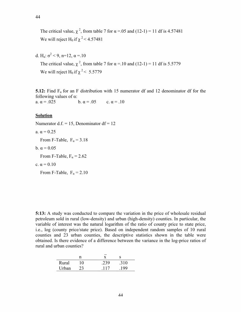
The critical value, χ 2, from table 7 for α =.05 and (12-1) = 11 df is 4.57481
We will reject H0 if χ 2 < 4.57481
d. Ha: σ2 < 9, n=12, α =.10
The critical value, χ 2, from table 7 for α =.10 and (12-1) = 11 df is 5.5779
We will reject H0 if χ 2 < 5.5779
5.12: Find Fα for an F distribution with 15 numerator df and 12 denominator df for the following values of α: a. α = .025 b. α = .05 c. α = .10
Solution
Numerator d.f. = 15, Denominator df = 12
a. α = 0.25
From F-Table, Fα = 3.18
b. α = 0.05
From F-Table, Fα = 2.62
c. α = 0.10
From F-Table, Fα = 2.10
5:13: A study was conducted to compare the variation in the price of wholesale residual petroleum sold in rural (low-density) and urban (high-density) counties. In particular, the variable of interest was the natural logarithm of the ratio of county price to state price, i.e., log (county price/state price). Based on independent random samples of 10 rural counties and 23 urban counties, the descriptive statistics shown in the table were obtained. Is there evidence of a difference between the variance in the log-price ratios of rural and urban counties?
n x s Rural 10 .239 .310 Urban 23 .117 .199

45
45
Solution
Let
σ12 = Log price variance for rural counties
σ22 = Log price variance for urban counties.
The elements of the two tailed hypothesis test are:
H0: σ12 / σ2
2 = 1
Ha: σ12 / σ2
2 ≠ 1
Test statistic F = Larger s2/ Smaller s2
= s12/ s2
2
= (.310) 2/ (.199) 2
= 2.4267,
for the two-tailed test, we will use α = .10 and α/2 = .05, d.f. for numerator (10 -1) =9,
and d.f. for denominator (23 -1) = 22. Thus the rejection region from table 9 is:
Reject H0 if F > 2.34
since the test statistic F = 2.4267, falls in the rejection region, we fail to accept the null
hypothesis. Therefore at α = .10, the data provides sufficient evidence to indicate a
difference between log price ratios of rural and urban counties.
6. Analysis of Variance: Equality of Several Populations
6.1: Independent random samples were selected from two populations, with the results shown in the table.
Sample 1 Sample 2 10 12 7 8 8 13 11 10 10 10 9 11 9

46
46
a. Construct a line plot of the data. Do you think the data provide evidence of a
difference between the population means? b. Calculate MST. What type of variability is measured by this quantity? c. Calculate MSE. What type of variability is measured by this quantity? d. How many degrees of freedom are associated with MST? e. How many degrees of freedom are associated with MSE? f. Compute the test statistic appropriate for testing H0: µ1 = µ2 against the alternative
hypothesis that the two means differ. g. Summarize the results of parts b-f in an ANOVA table. h. Specify the rejection region, using the significance level of α = 05 i. Make the proper conclusion. How does this compare to your answer to part a?
Solution
a.
sample 1 sample 2 10 12 7 8 8 13 11 10 10 10 9 11 9
Sum 64 64 sample mean
9.14 10.67
Grand mean
9.90

47
47
Because the difference between the sample means is small relative to the variability
within the sample observations, the data does not give a clear evidence of difference
between µ1 and µ2.
b. Here n1 = 7, and n2 = 6 SST is calculated using the formula SST = n1(y1bar - ybar)2 + n2 (y2bar - ybar)2
= 7 * (9.14 - 9.90) 2 + 6* (10.67 - 9.90)2 = 7.55
MST = SST/(k -1) = 7.55/(2-1) = 7.55 MST measures the variability explained by the difference between the sample means of the two treatments.
c. SSE calculation shown in table below is based on the formula,
SSE = ∑ (yi1 - y1bar)2 + ∑ (yi2 - y2bar)2
SSE
Calculation
0.73 1.78 4.59 7.11 1.31 5.44 3.45 0.44 0.73 0.44 0.02 0.11 0.02
Total 10.86 15.33
SSE = 10.86 + 15.33 = 26.19 MSE = SSE/(n - k) = 26.19/(13 - 2)
= 2.38 MSE measures the unexplained variability - that is, it measures variability unexplained by the differences between the sample means of the two treatments.
d. MST has (k - 1) = 2 - 1 = 1 degree of freedom.

48
48
e. MSE has (n - k) = 13 - 2 = 11 degree of freedom. f. Test statistic, F = MST/MSE = 7.55/2.38 = 3.17 g.
The AVOVA table Source Degree
of freedom
Sum of squares
Mean Squares
F-Statistic
Among treatment means 1 7.55 7.55 3.17 Within Samples 11 26.19 2.38
Total 12 33.74 h. α = .05, v1 = 1, and v2=11 Therefore from table 9 of Appendix B, F.05 = 4.84, and the rejection region is F > F.05
= 4.84
i. Because the computed value is less than F.05 = 4.84, we will fail to reject the null hypothesis, and conclude that the data does not give sufficient evidence to show that the sample means are different. This concurs with the findings in (a).
6.2: Independent random samples were selected from three populations. The data are shown in the accompanying table, followed by a SAS printout of the analysis of variance.
Sample 1 Sample 2 Sample 3 2.1 4.4 1.1 3.3 2.6 .2 .2 3.0 2.0 1.9
Analysis of Variance Procedure Dependent Variable: Y Source DF Sum of
Squares Mean Square
F value Pr > F

49
49
Model 2 6.22183333 3.11091667 2.21 0.1798 Error 7 9.83416667 1.40488095 Corrected Total
9 16.05600000
R-Square 0.387508
C.V 56.98446
Root MSE 1.185277
Y Mean 2.08000000
Source DF Anova SS Mean
Square F value Pr > F
SAMPLE 2 6.22183333 3.11091667 2.21 0.1798
a. Locate the value of MST. What type of variability is measured by this quantity? b. Locate the value of MSE. What type of variability is measured by this quantity? c. How many degrees of freedom are associated with MST? d. How many degrees of freedom are associated with MSE? e. Locate the value of the test statistic for testing H0: µ1 = µ2 = µ3 against the
alternative hypothesis that at least one population mean is different from the other two.
f. Summarize the results of parts a-e in an ANOVA table. g. Specify the rejection region, using a significance level of α = .05. h. State the proper conclusion. i. Locate and interpret the p-value for the test of part e. Does this agree with your
answer to part h? Solution
a. The value of MST is 3.11091667. MST measures the variability explained by the difference between the sample means
of the two treatments.
b. The value of MSE is 1.40488095. MSE measures the unexplained variability - that is, it measures variability
unexplained by the differences between the sample means of the two treatments.
c. MST has 2 degree of freedom.
d. MSE has 7 degree of freedom.
e. The value of test statistic is the F-value of 2.21
f.

50
50
The AVOVA table Source Degree of
freedom Sum of squares
Mean Squares
F-Statistic
Among treatment means
2 6.22 3.11 2.21
Within Samples
7 9.83 1.40
Total 9 16.06 g. α = .05, v1 = 2, and v2=7 Therefore from table 9 of Appendix B, F.05 = 4.74, and the rejection region is F > F.05
= 4.74
h. Because the computed value is less than F.05 = 4.74, we will fail to reject the null hypothesis,
and conclude that the data does not give sufficient evidence to show that the sample means are different.
i. P-value, p(Z > 2.21) = 1 - p(Z < 2.21) = 1 - .4864 = .5136 Because the observed p-value is greater than the fixed significance level, α = .05, we will fail to reject the null hypothesis. This concurs with the answer to part (h).
6.3: A few weeks after the end of each academic semester, the career Resource center (CRC) at University of Florida mails out questionnaires pertaining to the employment status and starting salary of all students gradating that particular semester. This information is used to compare the mean starting salaries of graduates of the various university colleges. The following table lists the starting salaries of independent random samples of eight graduates selected from each of five colleges – Business Administration, Education, Engineering, Liberal Arts and Sciences. Business Administration
Education
Engineering
Liberal Arts
Sciences
$13,400 $12,400 $27,200 $9,600 $15,200 23,400 14,700 16,000 11,300 20,300 15,100 11,500 29,200 12,800 15,600 22,900 21,800 24,400 10,700 14,400 18,000 7,700 25,700 13,100 18,100 19,300 11,900 18,000 17,800 14,800 22,600 10,700 21,900 12,600 15,900 18,100 6,100 25,700 21,600 15,200

51
51
To perform the comparison, the data were subjected to an analysis of variance using SPSS. The SPSS printout appears here. ------------------------------ONEWAY---------------------------------------------- Variable SALARY By Variable COLLEGE
Analysis of Variance Procedure Source D.F. Sum of
Squares Mean Squares
F Ratio F Prob.
Between Groups 4 659451500.0 164862875.0 10.6550 .0000 Within Groups 35 541546250.0 15472750.00 Total 39 1200997750
a. Give the null and alternative hypotheses appropriate for this analysis. b. Find the value of the test statistic. c. Do the data provide evidence of a difference in mean starting salaries among the
five colleges? (Interpret the p-value for the test) d. Estimate the difference between the mean starting salaries of Business
Administration and Engineering graduates at the University of Florida using a 95% confidence interval.
Solution
a. Our objective is to determine if there are any differences in starting salaries of
graduates of the various university colleges. Let µ1, µ2, µ3, µ4, and µ5 be the mean salaries of the five colleges. Therefore the null and alternate hypotheses are: H0 : µ1= µ2 = µ3 = µ4 = µ5 Ha : At least two mean salaries are different.
b. Test statistic, F = MST/MSE The values of MST, and MSE from the SPSS printout are 1.64862875.0 and 15472750.0 Substituting these values in the above formula, we get F = 164862875.0 / 15472750.0 = 10.6550
52
52
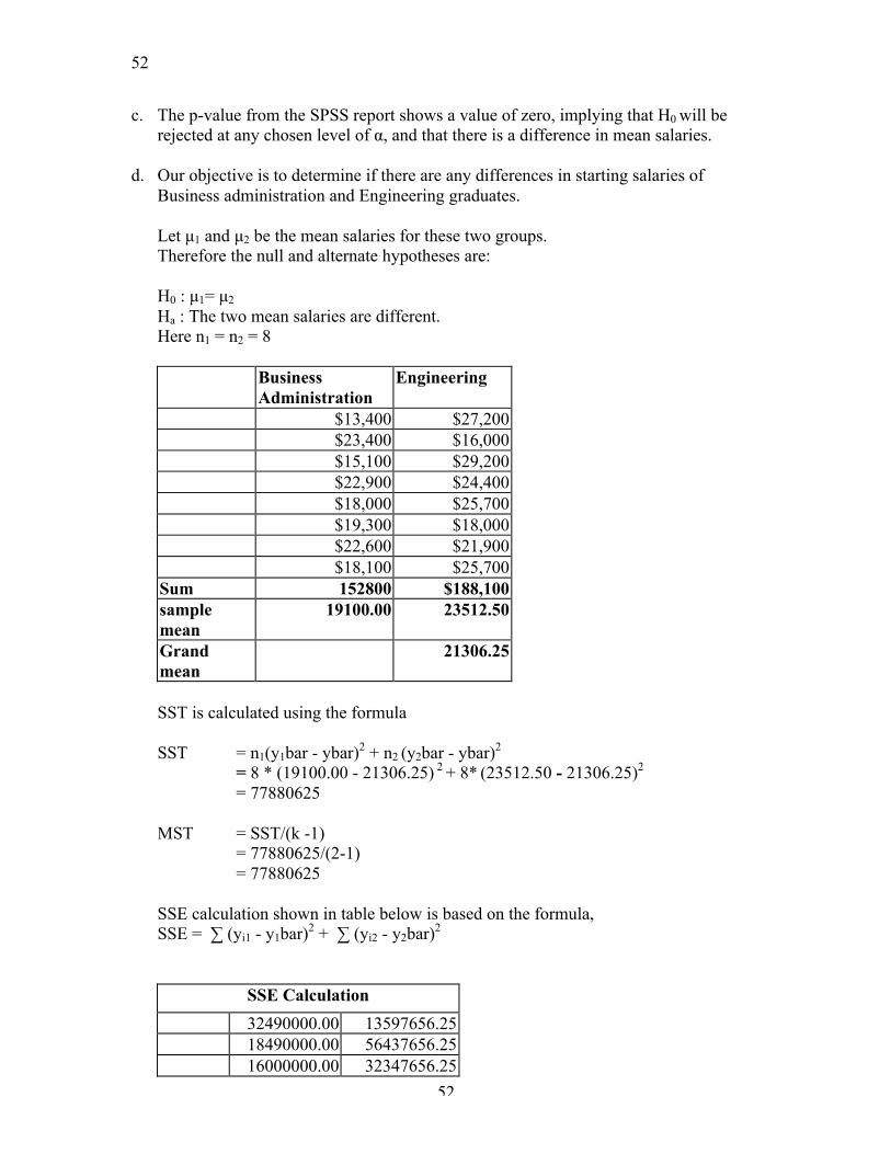
c. The p-value from the SPSS report shows a value of zero, implying that H0 will be rejected at any chosen level of α, and that there is a difference in mean salaries.
d. Our objective is to determine if there are any differences in starting salaries of Business administration and Engineering graduates.
Let µ1 and µ2 be the mean salaries for these two groups. Therefore the null and alternate hypotheses are: H0 : µ1= µ2 Ha : The two mean salaries are different. Here n1 = n2 = 8
Business Administration
Engineering
$13,400 $27,200 $23,400 $16,000 $15,100 $29,200 $22,900 $24,400 $18,000 $25,700 $19,300 $18,000 $22,600 $21,900 $18,100 $25,700
Sum 152800 $188,100 sample mean
19100.00 23512.50
Grand mean
21306.25
SST is calculated using the formula SST = n1(y1bar - ybar)2 + n2 (y2bar - ybar)2
= 8 * (19100.00 - 21306.25) 2 + 8* (23512.50 - 21306.25)2 = 77880625
MST = SST/(k -1) = 77880625/(2-1) = 77880625
SSE calculation shown in table below is based on the formula, SSE = ∑ (yi1 - y1bar)2 + ∑ (yi2 - y2bar)2
SSE Calculation 32490000.00 13597656.25 18490000.00 56437656.25 16000000.00 32347656.25

53
53
14440000.00 787656.25 1210000.00 4785156.25 40000.00 30387656.25 12250000.00 2600156.25 1000000.00 4785156.25
Total 95920000.00 145728750.00
SSE = 95920000.00 + 145728750.00 = 241648750
MSE = SSE/(n - k) = 241648750/(16 - 2)
= 17260625 Test statistic, F = MST/MSE = 77880625/17260625
= 4.51 MST has (k - 1) = 2 - 1 = 1 degree of freedom. MSE has (n - k) = 16 - 2 = 14 degree of freedom. The AVONA table is shown below.
The AVOVA table Source Degree of
freedom
Sum of squares
Mean Squares
F Statisti
c Among treatment means 1 77880625.00 77880625.00 4.51 Within Samples 14 241648750.00 17260625.00
Total 15 319529375.00 α = .05, v1 = 1, and v2=14
Therefore from table 9 of Appendix B, F.05 = 4.60, and the rejection region is F > F.05 = 4.60
Because the computed value of F = 4.51, is less than F.05 = 4.60, at 95% confidence,
we will fail to reject the null hypothesis, and conclude that the data does not give
sufficient evidence to show that the mean salaries are different.

54
54
7. Linear Regression with Applications 7.1: Consider the five data points:
x -1 0 1 2 3 y -1 1 1 2.5 3.5
a. Construct a scatter diagram for the data. b. Find the least squares prediction equation c. Graph the least squares line on the scatter diagram and visually confirm that it
provides a good fit to the data points.
Solution
a.
x -1 0 1 2 3 y -1 1 1 2.5 3.5
The scatter diagram for the above data is shown below:
b. Sum of squares for the above data is shown in the table below:

55
55
x y x2 x.y y2 -1 -1 1 1 1 0 1 0 0 1 1 1 1 1 1 2 2.5 4 5 6.25 3 3.5 9 10.5 12.25
∑x=5 ∑y=7 ∑x2=15 ∑xy=17.5 ∑y2=21.5
Here n = 5, therefore
SSxy = ∑xy - (∑x)( ∑y)/n = 17.5 - (5)(7)/5 = 10.5
SSxx = ∑x2 - (∑x)2/n = 15 - (5)2/5 = 10 Slope, β1 = SSxy/SSxx
= 10.5/10= 1.05
Y-intercept, β0 = ybar - β1 xbar = 7/5 - 1.05(5/5)= 0.35
The least square prediction equation is y = 0.35 + 1.05x
c. Since the y-intercept is .35, and because the least square line will always pass through
the point (Xbar,Ybar)= (1,1.4), the least square line is as shown below.
Because two of the five points lie on the line and because the individual deviations of the other points are small, we can consider this a good fit.

56
56
7.2: The data for exercise 7.1. are reproduced here.
x -1 0 1 2 3 y -1 1 1 2.5 3.5
a. Calculate SSE for the data. b. Calculate s² and s.
Solution
a. SSyy = ∑y2 - (∑y)2/n = 21.5 - (7) 2/5 = 11.7 Using value of β1=1.05 and SSxy =10.5 from the above problem, we can calculate SSE
using the formula: SSE = SSyy - β1 SSxy = 11.7 - 1.05 (10.5) = 0.675
b. s2 = SSE/(n - 2) = 0.675/(5 - 2) = 0.225
S = √S = √0.225 = 0.474342
7.3: The data for exercise 17.1 and 7.2 are reproduced here.
x -1 0 1 2 3 y -1 1 1 2.5 3.5
a. Test the null hypothesis that the slope β1 of the line equals 0 against the
alternative hypothesis that β1 is not equal to 0. Use α = .10 b. Compute the approximate observed significance level of the test. c. Find a 90% confidence interval for the slope β1.
Solution
a. The test hypotheses are: H0: β1 = 0
Ha: β1 ≠ 0
When n=5 and α = .10, the critical value based on (5 - 2) = 3 df is obtained from table 6 of appendix B: tα/2 = t.05 = 2.353
Thus we will reject the null hypothesis H0 if |t| > 2.353.

57
57
Using the values of β1= 1.05, s=0.474342, and SSxx = 0.474342 from the above solutions, we can calculate the test statistic as follows.
t = β1/(s/√SSxx) = 1.05 /(0.474342/√10) = 6.999995
Since the calculated t value falls in the rejection region, we will reject the null hypothesis and conclude that the slope β1 is not 0.
b. The observed significance level of the test is P=0.005986 c. We can calculate the 90% confidence interval using the formula β1 + tα/2 (s/√SSxx) When n=5 and α = .10, the critical value based on (5 - 2) = 3 df is obtained from table
6 of appendix B: tα/2 = t.05 = 2.353 β1 + tα/2 (s/√SSxx) = 1.05 + 2.353 (0.474342/√10) = 1.05 + 0.35295 Therefore confidence interval is 0.69705 to 1.40295.
7.4: Give an Example of two economic or business variables that are: a. Positively correlated b. Negatively correlated.
Solution
a. Retail sales growth is positively correlated with gross domestic product (GDP) growth. b. Sales are negatively correlated with net price levels.
7.5: Refer to data of Exercises 7.1-7.3. Calculate the coefficient of determination r2 and interpret its value.
Solution
The coefficient of determination, r2, is calculated using the formula
r2 = (SSyy - SSE)/ SSyy
From previous solution we have SSyy = 11.7 and SSE = 0.675. Substituting these values
in the above equation we have,
r2 = (11.7 - 0.675)/11.7 = 0.9423
58
58
We interpret this value as follows: The use of value x, to predict value y with the least
square line accounts for approximately 94% of the total sum of squares of deviations
of the five sample y values about their mean.
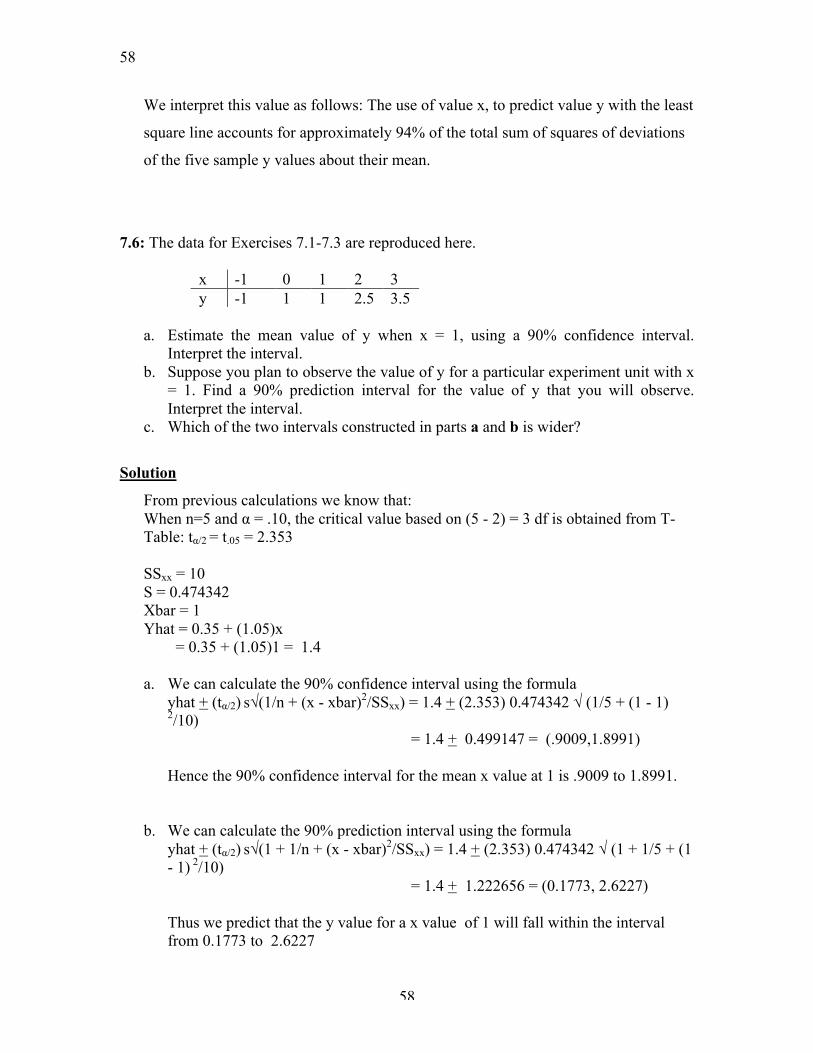
7.6: The data for Exercises 7.1-7.3 are reproduced here.
x -1 0 1 2 3 y -1 1 1 2.5 3.5
a. Estimate the mean value of y when x = 1, using a 90% confidence interval.
Interpret the interval. b. Suppose you plan to observe the value of y for a particular experiment unit with x
= 1. Find a 90% prediction interval for the value of y that you will observe. Interpret the interval.
c. Which of the two intervals constructed in parts a and b is wider?
Solution
From previous calculations we know that: When n=5 and α = .10, the critical value based on (5 - 2) = 3 df is obtained from T-Table: tα/2 = t.05 = 2.353 SSxx = 10 S = 0.474342 Xbar = 1 Yhat = 0.35 + (1.05)x
= 0.35 + (1.05)1 = 1.4
a. We can calculate the 90% confidence interval using the formula yhat + (tα/2) s√(1/n + (x - xbar)2/SSxx) = 1.4 + (2.353) 0.474342 √ (1/5 + (1 - 1)
2/10) = 1.4 + 0.499147 = (.9009,1.8991) Hence the 90% confidence interval for the mean x value at 1 is .9009 to 1.8991.
b. We can calculate the 90% prediction interval using the formula yhat + (tα/2) s√(1 + 1/n + (x - xbar)2/SSxx) = 1.4 + (2.353) 0.474342 √ (1 + 1/5 + (1 - 1) 2/10) = 1.4 + 1.222656 = (0.1773, 2.6227) Thus we predict that the y value for a x value of 1 will fall within the interval from 0.1773 to 2.6227

59
59
c. The prediction interval is wider than the confidence interval.