title: nikon a1plus confocal user manual - … · title: nikon a1plus confocal user manual date of...
TRANSCRIPT
Title: Nikon A1Plus Confocal User Manual
Date of first issue:
23/10/2015
Date of review: 26/09/2016 Version:
V2 Admin
For assistance or to report an issue
Office: CG.07 or CG.05
Email: [email protected]
Website: www.igmm-imaging.com
Download a PDF copy of manual:
\\smbhost\microscope-users\microscope user manuals\Nikon A1Plus
Facility Usage Policy
1. You must have the relevant Risk Assessment/COSHH form for the work you are undertaking before using imaging facility resources
2. Users must be trained before using facility equipment
3. Please leave the microscope clean and tidy for the next user
4. Please report any issue, even if it seems minor, to facility staff
5. Any clinical waste must be placed in the orange bins provided
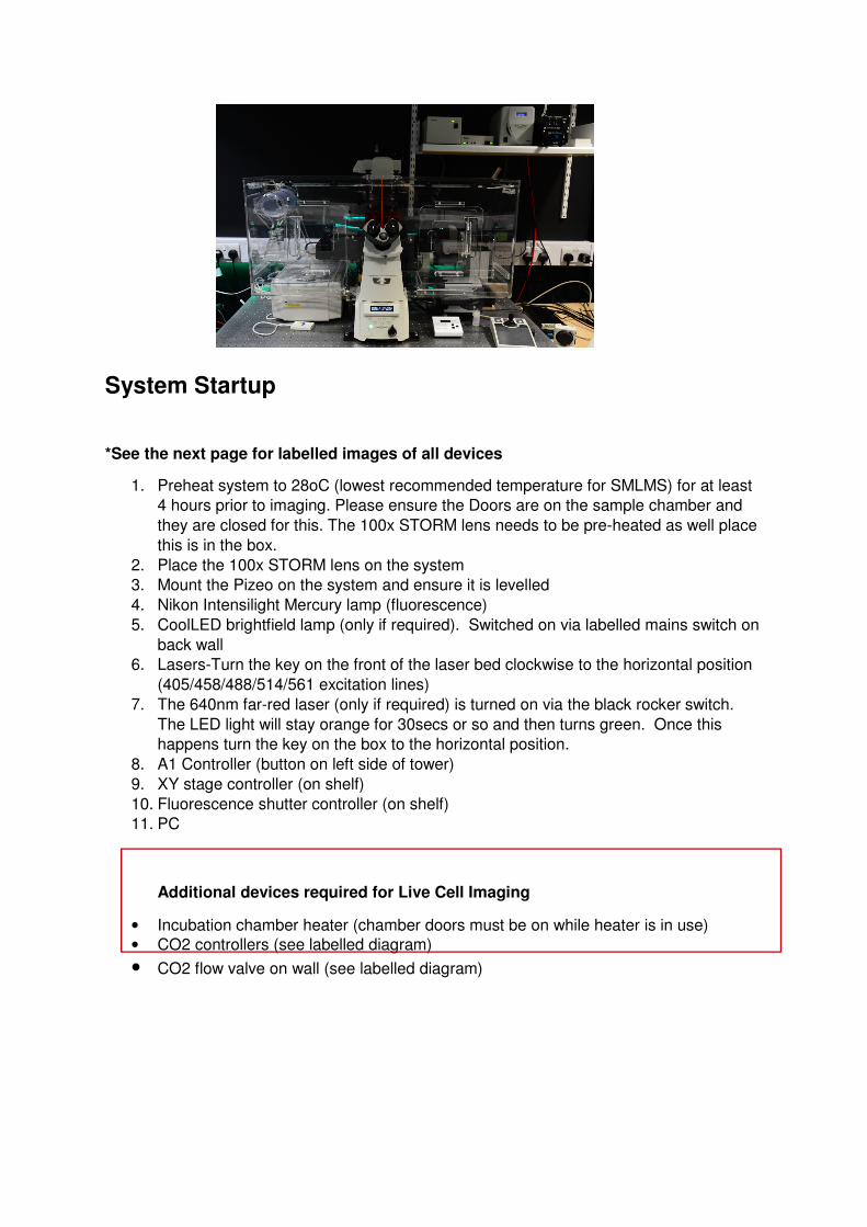
System Startup
*See the next page for labelled images of all devices
1. Preheat system to 28oC (lowest recommended temperature for SMLMS) for at least
4 hours prior to imaging. Please ensure the Doors are on the sample chamber and
they are closed for this. The 100x STORM lens needs to be pre-heated as well place
this is in the box.
2. Place the 100x STORM lens on the system
3. Mount the Pizeo on the system and ensure it is levelled
4. Nikon Intensilight Mercury lamp (fluorescence)
5. CoolLED brightfield lamp (only if required). Switched on via labelled mains switch on
back wall
6. Lasers-Turn the key on the front of the laser bed clockwise to the horizontal position
(405/458/488/514/561 excitation lines)
7. The 640nm far-red laser (only if required) is turned on via the black rocker switch.
The LED light will stay orange for 30secs or so and then turns green. Once this
happens turn the key on the box to the horizontal position.
8. A1 Controller (button on left side of tower)
9. XY stage controller (on shelf)
10. Fluorescence shutter controller (on shelf)
11. PC
Additional devices required for Live Cell Imaging
• Incubation chamber heater (chamber doors must be on while heater is in use)
• CO2 controllers (see labelled diagram)
• CO2 flow valve on wall (see labelled diagram)

1. Log in to Windows using the “User” account
2. If using the 640nm laser launch its control software from the desktop icon
3. Select the Power mW button and type 3 into the text box
4. Press the “On” button
5. You can minimise the Fiber laser window but don't close it
6. Launch Nis-Elements from the desktop icon. If you have been trained then you will have a username to log in to Elements
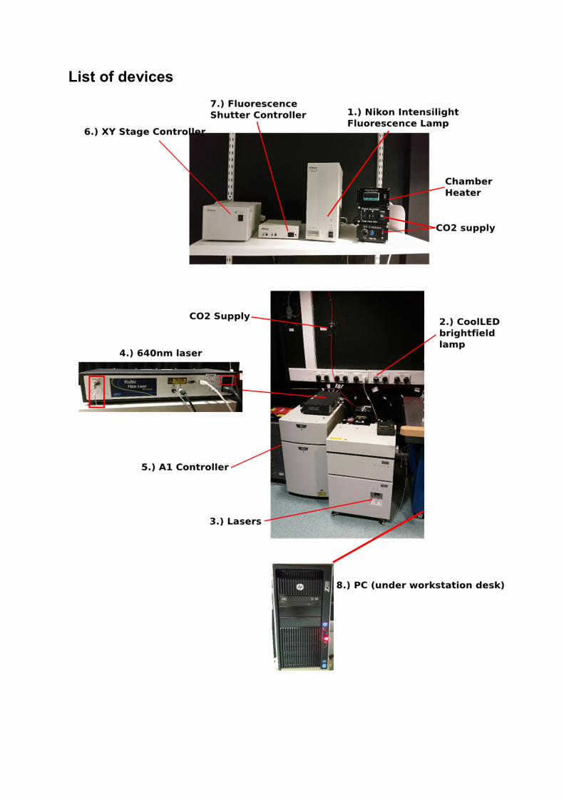
List of devices

System Shutdown
1. Clean any oil immersion lenses used with the lens tissue 2. Close Nikon Nis-Elements 3. If the 640nm laser is turned on, maximise the 640 control software and select Off
then close the window 4. Shutdown the PC
Incubation chamber heater and CO2 supply if used
5. Fluorescence shutter controller (on shelf) 6. XY stage controller (on shelf) 7. A1 Controller 8. CoolLED brightfield lamp, Switched off via labelled mains switch on back wall 9. Lasers Turn the key on the front of the laser bed anticlockwise to the vertical position
10. Nikon Intensilight Mercury lamp (fluorescence)
Mounting a sample
1. Ensure the correct stage insert is mounted (see facility staff if unsure)
2. Select a low magnification (10-20x) lens from the touchpad objective menu
3. Use the joystick to move the stage if necessary. Change the speed of the stage by twisting the joystick.
4. Before mounting the slide on the stage, turn the microscope focus knob, if the Z value on the microscopes front LCD display doesn't change as you turn, the lens is in the Escape position. Press the Refocus button on the right side of the microscope body.
5. Remember to invert your slide so that the cover glass is the closest surface to the lens

ALIGN TIRF Illumination
1) Launch 647 laser
Launch GUI-VFL software
Press On
Press Activate
The TIRF illumination will need to be aligned, initially set the power to
30mw for alignment (see below).
For SMLM imaging power of between 100 and 300mw is recommended.
2) Launch NIS Elements
3) Align the TIRF illumination:

4) Locate the sample (1 colour 647)
i) To find the sample by eye select the Eyes options. Ensure
the sample is in the very centre of the field of view. If
included use the fiducial marker to locate the sample.
ii) Switch on the Perfect focus system
To locate the sample on the camera select STORM 647 which will
go into TIRF illumination or STORM-647 HiLo which will use near
TIRF.
iii) Set up the camera, Ensure the setting are
a. Readout mode: EM Gain 17MHz at 16 bit
b. EM Gain Multiplier: 300
c. Conversion Gain: 3
d. Adjust autoexposure, generally 1 frame is ok.
iv) Visualise the sample on the camersa
a. Press the Green Arrow in the top menu
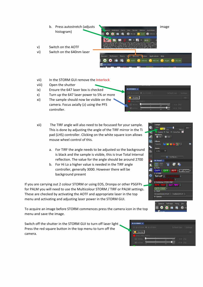
b. Press autostretch (adjusts image
histogram)
v) Switch on the AOTF
vi) Switch on the 640nm laser
vii) In the STORM GUI remove the Interlock
viii) Open the shutter
ix) Ensure the 647 laser box is checked
x) Turn up the 647 laser power to 5% or more
xi) The sample should now be visible on the
camera. Focus axially (z) using the PFS
controller.
xii) The TIRF angle will also need to be focussed for your sample.
This is done by adjusting the angle of the TIRF mirror in the Ti
pad (LHS) controller. Clicking on the white square icon allows
mouse wheel control of this.
a. For TIRF the angle needs to be adjusted so the background
is black and the sample is visible, this is true Total Internal
reflection. The value for the angle should be around 2700
b. For Hi Lo a higher value is needed in the TIRF angle
controller, generally 3000. However there will be
background present
If you are carrying out 2 colour STORM or using EOS, Dronpa or other PSGFPs
for PALM you will need to use the Multicolour STORM / TIRF or PALM settings.
These are checked by activating the AOTF and appropriate laser in the top
menu and activating and adjusting laser power in the STORM GUI.
To acquire an image before STORM commences press the camera icon in the top
menu and save the image.
Switch off the shutter in the STORM GUI to turn off laser light
Press the red square button in the top menu to turn off the
camera.
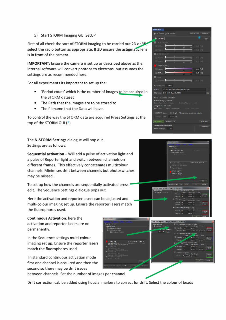
5) Start STORM Imaging GUI SetUP
First of all check the sort of STORM imaging to be carried out 2D or 3D,
select the radio button as appropriate. If 3D ensure the astigmatic lens
is in front of the camera.
IMPORTANT: Ensure the camera is set up as described above as the
internal software will convert photons to electrons, but assumes the
settings are as recommended here.
For all experiments its important to set up the:
• ‘Period count’ which is the number of images to be acquired in
the STORM dataset
• The Path that the images are to be stored to
• The filename that the Data will have.
To control the way the STORM data are acquired Press Settings at the
top of the STORM GUI (*)
The N-STORM Settings dialogue will pop out.
Settings are as follows:
Sequential activation – Will add a pulse of activation light and
a pulse of Reporter light and switch between channels on
different frames. This effectively concatenates multicolour
channels. Minimises drift between channels but photoswitches
may be missed.
To set up how the channels are sequentially activated press
edit. The Sequence Settings dialogue pops out
Here the activation and reporter lasers can be adjusted and
multi-colour imaging set up. Ensure the reporter lasers match
the fluorophores used.
Continuous Activation: here the
activation and reporter lasers are on
permanently.
In the Sequence settings multi-colour
imaging set up. Ensure the reporter lasers
match the fluorophores used.
In standard continuous activation mode
first one channel is acquired and then the
second so there may be drift issues
between channels. Set the number of images per channel
Drift correction cab be added using fiducial markers to correct for drift. Select the colour of beads
*
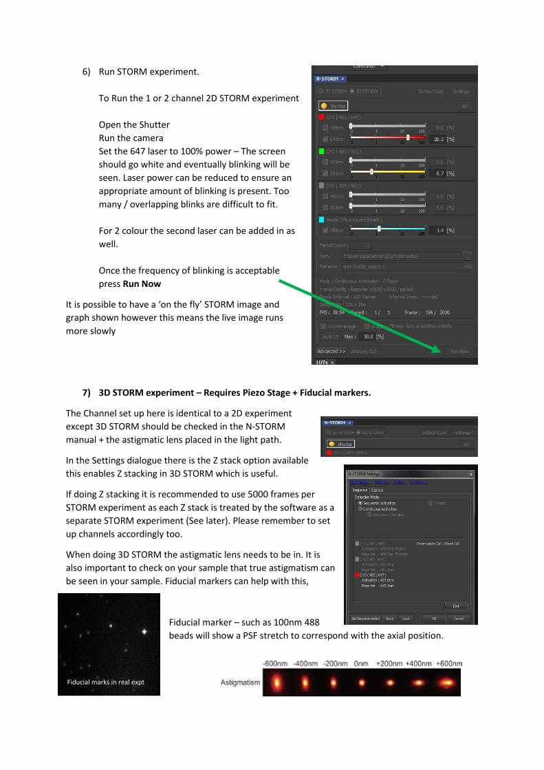
6) Run STORM experiment.
To Run the 1 or 2 channel 2D STORM experiment
Open the Shutter
Run the camera
Set the 647 laser to 100% power – The screen
should go white and eventually blinking will be
seen. Laser power can be reduced to ensure an
appropriate amount of blinking is present. Too
many / overlapping blinks are difficult to fit.
For 2 colour the second laser can be added in as
well.
Once the frequency of blinking is acceptable
press Run Now
It is possible to have a ‘on the fly’ STORM image and
graph shown however this means the live image runs
more slowly
7) 3D STORM experiment – Requires Piezo Stage + Fiducial markers.
The Channel set up here is identical to a 2D experiment
except 3D STORM should be checked in the N-STORM
manual + the astigmatic lens placed in the light path.
In the Settings dialogue there is the Z stack option available
this enables Z stacking in 3D STORM which is useful.
If doing Z stacking it is recommended to use 5000 frames per
STORM experiment as each Z stack is treated by the software as a
separate STORM experiment (See later). Please remember to set
up channels accordingly too.
When doing 3D STORM the astigmatic lens needs to be in. It is
also important to check on your sample that true astigmatism can
be seen in your sample. Fiducial markers can help with this,
Fiducial marker – such as 100nm 488
beads will show a PSF stretch to correspond with the axial position.
Fiducial marks in real expt
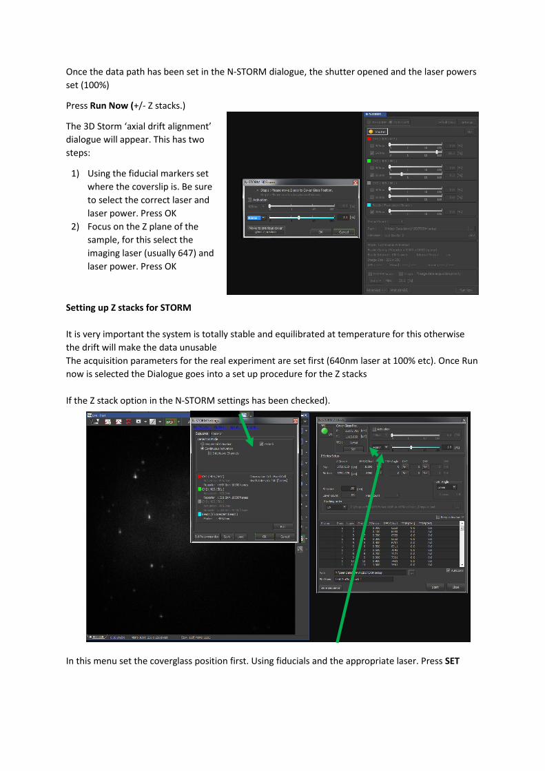
Once the data path has been set in the N-STORM dialogue, the shutter opened and the laser powers
set (100%)
Press Run Now (+/- Z stacks.)
The 3D Storm ‘axial drift alignment’
dialogue will appear. This has two
steps:
1) Using the fiducial markers set
where the coverslip is. Be sure
to select the correct laser and
laser power. Press OK
2) Focus on the Z plane of the
sample, for this select the
imaging laser (usually 647) and
laser power. Press OK
Setting up Z stacks for STORM
It is very important the system is totally stable and equilibrated at temperature for this otherwise
the drift will make the data unusable
The acquisition parameters for the real experiment are set first (640nm laser at 100% etc). Once Run
now is selected the Dialogue goes into a set up procedure for the Z stacks
If the Z stack option in the N-STORM settings has been checked).
In this menu set the coverglass position first. Using fiducials and the appropriate laser. Press SET

Next, the Z series is set up.
• This is done using the channel of interest so
the laser needs to be changed to the
imaging laser at low power.
• The Axial and TIRF angles are both set and
step size starting with the z position and
TIRF angle at the top (both are set using
separate SET buttons). Then the bottom z
position and TIRF angle (again both set
using appropriate SET buttons).
• The stacking order can be set and the TIRF
angle. I used Linear. The Path and Filename
of data are set. Then START is pressed.
• Acquistion of the data will now start.
Each Z stack is cycled through and on the dialogue it
is noted if the Z stack is capturing or finished.
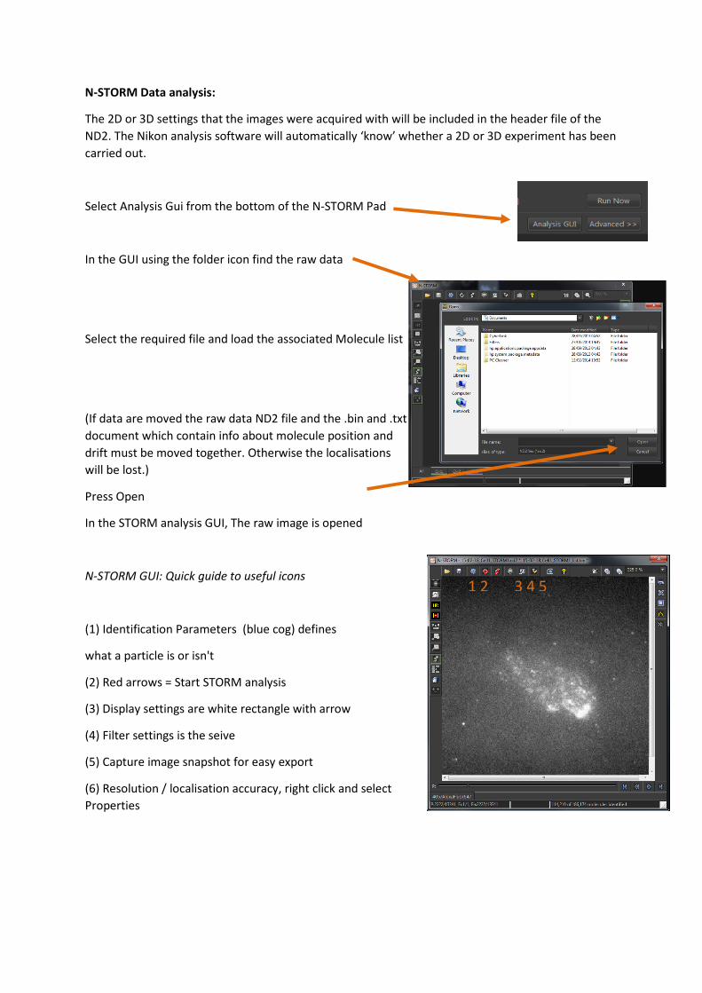
N-STORM Data analysis:
The 2D or 3D settings that the images were acquired with will be included in the header file of the
ND2. The Nikon analysis software will automatically ‘know’ whether a 2D or 3D experiment has been
carried out.
Select Analysis Gui from the bottom of the N-STORM Pad
In the GUI using the folder icon find the raw data
Select the required file and load the associated Molecule list
(If data are moved the raw data ND2 file and the .bin and .txt
document which contain info about molecule position and
drift must be moved together. Otherwise the localisations
will be lost.)
Press Open
In the STORM analysis GUI, The raw image is opened
N-STORM GUI: Quick guide to useful icons
(1) Identification Parameters (blue cog) defines
what a particle is or isn't
(2) Red arrows = Start STORM analysis
(3) Display settings are white rectangle with arrow
(4) Filter settings is the seive
(5) Capture image snapshot for easy export
(6) Resolution / localisation accuracy, right click and select
Properties
1 2 3 4 5

The 2D fitting is centroid fitting like QuickPALM (2)
When analysing a Storm experiment the ID settings need to be carefully set up.Press
the blue cog to open the Identification settings GUI. In the ‘Start STORM Analysis’
dialogue box press Identification Settings to optimise how the photoswitching
molecules are identified.
It is recommended that the ROI is autofitted. To define the
parameters for autofitting press >> (*)
Expands showing the Screening menu.
This allows definition of the minimum and maximum width
expected of a fluorophore blink
The initial fit width (i.e. how large the expected diffraction
limited blink is) and the expected discrepancy in the ratio in
the x and y plane (fit tolerance).
The centroid fitting cannot cope with overlapping blinks
from 2 or more fluorophores and rejects them.
If the structure is filamentous or densely labelled the centroid fitting will not work. Instead
overlapping pixels can be fitted by checking the box. This is multiple emitter fit code written by the
Zhuang lab (3) . This is slower.
For 3D STORM analysis the Auto Fit ROI should be checked. The Maximum
width should also be adjusted, initially try 800 and an axial ratio of 3
Once the ID settings have been set up they can be tested to see how well
they perform by pressing Test in the Start STORM analysis GUI
It is recommended that a period (i.e. frame) is chosen in the middle of the
experiment as there will be quite a few images which are too saturated
with blinks at the beginning to localise.
*

An example of localisations is shown (right)
False positives are indicated. (*)
These can be removed by adjustment of the Identification
setting parameters
False negatives (i.e. blinks which aren’t identified by the
system – can be corrected for by refining the ID settings
N.B. To remove the yellow squares the icon on the LHS menu
with a yellow square around it can be pressed.
The data to be analysed can be cropped in the
analysis window by right clicking at the bottom of
the image on the frame and selecting the start
and end period to analyse
To start the STORM analysis once the experiment is complete
press Start in the Storm Analysis gui
This will automatically start processing the image and generate an output image which is an overlay
of the low resolution STORM image and the high resolution fitting.
*
*

Post processing the 2D/3D STORM image
The processed STORM image (right) consists of dots, these indicate blinks and their size and shape
depend on the localisation accuracy which can be adjusted.
(1A) Correct system drift: Drift can be corrected by pressing the drift correction button. If the system
has fiducials + these have been detected these are used. Otherwise an autocorrelation algorithm
corrects dirft
The drift correction can be applied or removed once calculated using the snake icon in the LHS menu
(1B) If the first few frames are saturated these can be
removed from the analysis so only the photo-switching
events are analysed
The data to be analysed can be cropped in the analysis
window by right clicking at the bottom of the image on
the frame and selecting the start and end period to analyse
(2) Remove false positive localisations:
An example of localisations is shown (right)
False positives are indicated (*)
These can be removed by adjustment of the Identification
setting parameters
False negatives (i.e. blinks which aren’t identified by the
system (Purple arrow) can be corrected for by refining
the ID settings
N.B. To remove the yellow squares the icon on the LHS
menu with a yellow square around it can be pressed.
*
*
*
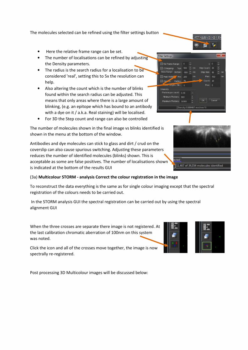
The molecules selected can be refined using the filter settings button
• Here the relative frame range can be set.
• The number of localisations can be refined by adjusting
the Density parameters.
• The radius is the search radius for a localisation to be
considered 'real', setting this to 5x the resolution can
help.
• Also altering the count which is the number of blinks
found within the search radius can be adjusted. This
means that only areas where there is a large amount of
blinking, (e.g. an epitope which has bound to an antibody
with a dye on it / a.k.a. Real staining) will be localised.
• For 3D the Step count and range can also be controlled
The number of molecules shown in the final image vs blinks identified is
shown in the menu at the bottom of the window.
Antibodies and dye molecules can stick to glass and dirt / crud on the
coverslip can also cause spurious switching. Adjusting these parameters
reduces the number of identified molecules (blinks) shown. This is
acceptable as some are false positives. The number of localisations shown
is indicated at the bottom of the results GUI
(3a) Multicolour STORM - analysis Correct the colour registration in the image
To reconstruct the data everything is the same as for single colour imaging except that the spectral
registration of the colours needs to be carried out.
In the STORM analysis GUI the spectral registration can be carried out by using the spectral
alignment GUI
When the three crosses are separate there image is not registered. At
the last calibration chromatic aberration of 100nm on this system
was noted.
Click the icon and all of the crosses move together, the image is now
spectrally re-registered.
Post processing 3D Multicolour images will be discussed below:

(4) Determine localisation precision (standard error of fitting) to do this the photons per count
should be entered into this box. They can be calculated the following information:
Photons per count calibration (filter settings STORM GUI)
Use Andor DU897 camera settings:
• EM gain 17MHz at 16-bit
• Conversion gain of 3
• Photons per count = 4.85/EM gain
(5) Export all the information about localisations right click in the STORM imaging analysis menu
It is essential when images are reported in the literature that they contain not only a scale bar but
also information about the error of localisation as this depends on how much light is collected. This
data also should be kept in case of editors questions
NB Error of precision must not be used until the calibration for photons per intensity count has been
entered into the filter settings menu as an incorrect value will invalidate the
equation (see Betzig Science 2006 for more info about how the maths
works)
The information about the STORM experiment can be saved by right
clicking in the STORM image and choosing properties.
Information about the Experiment, the positions of the
molecules and statistics is kept here. This file should be saved
for each experiment.
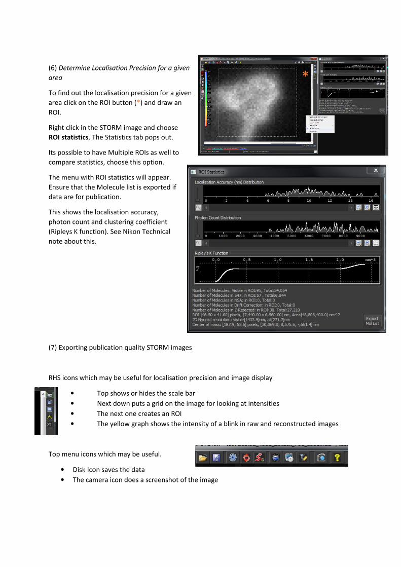
(6) Determine Localisation Precision for a given
area
To find out the localisation precision for a given
area click on the ROI button (*) and draw an
ROI.
Right click in the STORM image and choose
ROI statistics. The Statistics tab pops out.
Its possible to have Multiple ROIs as well to
compare statistics, choose this option.
The menu with ROI statistics will appear.
Ensure that the Molecule list is exported if
data are for publication.
This shows the localisation accuracy,
photon count and clustering coefficient
(Ripleys K function). See Nikon Technical
note about this.
(7) Exporting publication quality STORM images
RHS icons which may be useful for localisation precision and image display
• Top shows or hides the scale bar
• Next down puts a grid on the image for looking at intensities
• The next one creates an ROI
• The yellow graph shows the intensity of a blink in raw and reconstructed images
Top menu icons which may be useful.
• Disk Icon saves the data
• The camera icon does a screenshot of the image
*

Post processing the 3D multicolour STORM image
The output image shows the Z information which was
included and excluded. The Axial (3D) drift needs to be
corrected using drift correction:
LHS Icons:
• 3D drift correction
• For depth coding the 3D image,
• For controlling 3D in time
• Batch process
• 3D Volume viewer
• Colour correction of the 3D image
3D display of the STORM image can be visualised by pressing the 3D
volume icon
(top menu)
• In the 3D viewer you can control the display of the rendered
image. The camera icon allows the output to be stored.
• The camcorder allows a movie to be taken.
• The crosses for localisation can be viewed.
• Different planes (X, Y or Z can be visualised using the View
tab).
To change the depth coding in the image Right click the Depth coding icon
Here Height map can be selected/
By pressing the Advanced tab the
look up table for the height map
By changing the Min + Max and
colours in the box the 3D rendering
colours alter and a scale coding
depth intensity (LHS) appears
The z rejected blinks (because they
were a funny shape) are shown or
hidden here and the height map
can be toggled on and off.
Data should be exported in the
same way as a 2D imaging

N-STORM Analysis Tools:
Filter Settings (Density)
Density: This is a density based filter whose main purpose is to clean up the background
localizations outside of the structure of interest. It is implemented using publicized DBSCAN
algorithm. The algorithm groups points into clusters by exploring their topological relationships.
The filter can be enabled or disabled with its check box. Just like its underlying algorithm it
requires two parameters: Radius and Count. Radius is the max neighborhood search radius. Count is the min count for a group of points to
form a cluster. Points that don’t form clusters of required density are considered noise and get
hidden. Density filter is applied last. This allows all other filters to form the input for the density
filter. This filter is interactive. Its effect can be visible without closing Filter Settings dialog.
Radius and Count can be changed by either typing new values followed by Enter or via mouse
scroll wheel while the cursor is hovering over the corresponding edit box. The adjustment range
and acceleration options can be found in the tooltips.
The status bar at the bottom of the Filter Settings dialog pertains to Density Filter. The right
pane displays the density calculated as the ratio of the current count over the round area for
2D data (or over the sphere volume for 3D) with current radius. Double clicking the right pane
toggles the area or volume units between nanometers and micrometers (squared or cubed
correspondingly). As the radius and count are adjusted the density is recalculated.
N-STORM Analysis Tools:
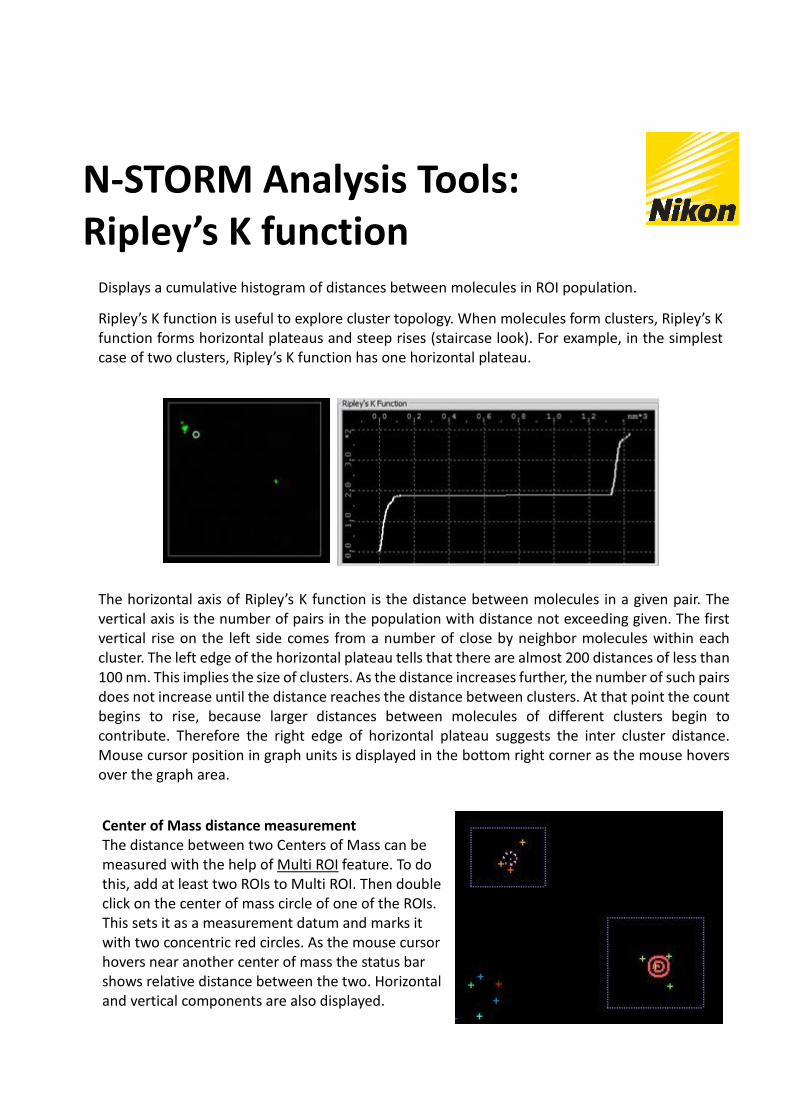
Ripley’s K function
Displays a cumulative histogram of distances between molecules in ROI population.
Ripley’s K function is useful to explore cluster topology. When molecules form clusters, Ripley’s K
function forms horizontal plateaus and steep rises (staircase look). For example, in the simplest
case of two clusters, Ripley’s K function has one horizontal plateau.
The horizontal axis of Ripley’s K function is the distance between molecules in a given pair. The
vertical axis is the number of pairs in the population with distance not exceeding given. The first
vertical rise on the left side comes from a number of close by neighbor molecules within each
cluster. The left edge of the horizontal plateau tells that there are almost 200 distances of less than
100 nm. This implies the size of clusters. As the distance increases further, the number of such pairs
does not increase until the distance reaches the distance between clusters. At that point the count
begins to rise, because larger distances between molecules of different clusters begin to
contribute. Therefore the right edge of horizontal plateau suggests the inter cluster distance.
Mouse cursor position in graph units is displayed in the bottom right corner as the mouse hovers
over the graph area.
Center of Mass distance measurement The distance between two Centers of Mass can be
measured with the help of Multi ROI feature. To do
this, add at least two ROIs to Multi ROI. Then double
click on the center of mass circle of one of the ROIs.
This sets it as a measurement datum and marks it
with two concentric red circles. As the mouse cursor
hovers near another center of mass the status bar
shows relative distance between the two. Horizontal
and vertical components are also displayed.
