FLIM/FFS

FLIM & FFS UPGRADE FOR NIKON SYSTEMS

PHOTO CREDIT / NIKON

Laser scanning confocal microscopy provides a wealth of information in the life sciences (cell biology, genetics, physiology, neurobiology, and developmental biology), tissue engineering, quantum optics and material sciences.

Typically, the instrumentation uses the fluorescence emission properties to detect the presence of the fluorophores targeted for the measurement. Yet, if two distinct fluorophores emit the fluorescence in a similar wavelength range, their respective contributions cannot be individually resolved and separated; moreover, the intensity depends upon the concentration of the fluorophores.

Fluorescence LifetimeThe measurement of fluorescence decay times, or lifetime, addresses these limitations. What is the fluorescence lifetime of an ensemble of molecules? Assuming the molecules have absorbed photons, it is a measure of the average time they retain the photons before returning them as fluorescence. Using the quantum mechanics description of the energy levels of a molecule, a number (N) of fluorophores, upon absorption of photons, undergoes a jump from the ground level to the excited levels. From there, the fluorophores decay to the lowest of the excited levels; hence, they decay back to the ground level with emission of photons, or fluorescence. The decay is a random process occurring at different times for different molecules of the ensemble. If the process is described by a single exponential decay, the lifetime is the time for the population in the lowest excited level to decrease by about 63%; or, it is the time the number of molecules in the excited level decreases to 36% of its original value. Decay times range typically from 50 picoseconds to hundreds of nanoseconds (although there are processes shorter and longer).

The decay time of the fluorescence is a property peculiar to each fluorophore, therefore it can be used to identify the presence of two or more fluorophores in a mixture and separate their individual contributions to the overall fluorescence even if they have overlapping emission spectra. Moreover, within some wide range, the lifetime values are independent of the fluorophore concentration, a property than can be used in several experimental situation with great advantage.

The lifetime of a fluorophore is affected by the environment (pH, presence of ions, temperature, electrical fields, viscosity of the solution) and, for this unique property, several information can be inferred from its measurement. Moreover, the lifetime of a fluorophore is affected by the close presence of another fluorophore (a principle used in the Förster Resonance Energy Transfer, or FRET); the FRET measurement can be used to determine and quantify these interactions and determine the intramolecular distance.

The measurement of the decay time offers new potentialities for the understanding and quantification of molecular dynamics at a single XYZ point of a system under study using your Nikon A1 confocal microscope.

Fluorescence Lifetime Imaging Fluorescence Lifetime Imaging (FLIM) is a technique that allows for the determination, at each pixel of the image, of the decay times of the fluorophores imaged in the pixel. The FLIM data are analyzed by the user friendly VistaVision software using the fitting algorithm to present the lifetime image, that is an image where at each pixel of the image the values of the decay times are plotted.

Alternatively, VistaVision analyzes the decay rates using the phasor technique, an approach that greatly simplifies the FLIM analysis and provides the FRET efficiency in a direct straightforward way. In addition to the standard intensity measurements, FLIM opens another horizon of measurement capabilities for your Nikon A1 confocal microscope.

Why FLIM?

FLIM provides the following information:

• Protein-protein interactions

• Molecular interactions

• Conformational dynamics

• Protein folding

• Rotational motion information

(local viscosity)

• Oxygen concentration

• Ion concentrations (Ca++, Cl-)

• pH measurements in cells

• Molecular distances (through FRET)

2

Figure 1. An aminoacid rigid linker was built with a total of 5-, 17- and 32-bases, respectively. Cerulean (donor) was bound to one end and Venus (acceptor) to the other extremity of each linker, identified as C5V, C17V and C32V. Cells were expressed with the three different constructs; separate cells were expressed with Cerulean only. The figures, starting from the left top include the cell expressed with Cerulean only (blue); the C5v (red), the C17V (yellow) and the C32V (green). The lifetime of the Cerulean decreases as the number of bases decreases; moreover, an additional decay rate is present. This is shown on the phasor plot to the right, where the position of the pixels from each cell are enclosed by a circle of the respective color. Excitation wavelength was 440nm from a laser diode. Measurements were acquired on a Nikon Ti microscope using the CFI 60x/1.2 NA water objective. (courtesy of Dr. A. Periasamy, University of Virginia).

Figure 2. NADH in live cells displaying the intensity (top) and the lifetime (bottom). Analysis is conducted using the fitting algorithm (right), which provides two decay times, 310 ps (60%) and 4.35 ns (40%). The phasor plot (left) displays the NADH in solution (single exponential, 450 ps) and in the cell. Excitation wavelength was 375 nm from a laser diode; emission was acquired through a filter. Measurements were acquired on a Nikon Ti microscope using the CFI 60x/1.2 NA water objective.

R G S

0.040 0.399 0.481 50.32 0.624 3.20 3.32

En Color

0.020 0.535 0.451 40.14 0.700 2.24 2.71

0.020 0.575 0.428 36.62 0.717 1.97 2.58

0.020 0.617 0.409 33.59 0.740 1.76 2.41

The lifetime of the Cerulean decreases as the number of bases decreases; moreover, an additional decay rate is present.

3

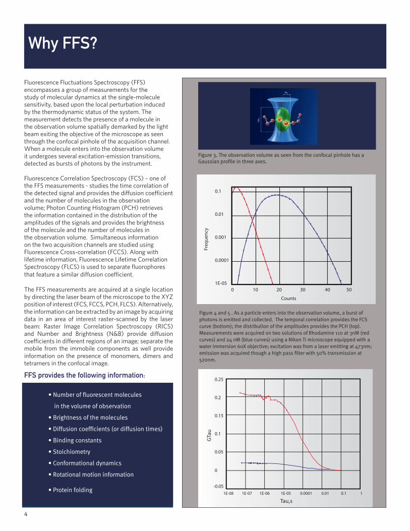
Fluorescence Fluctuations Spectroscopy (FFS) encompasses a group of measurements for the study of molecular dynamics at the single-molecule sensitivity, based upon the local perturbation induced by the thermodynamic status of the system. The measurement detects the presence of a molecule in the observation volume spatially demarked by the light beam exiting the objective of the microscope as seen through the confocal pinhole of the acquisition channel. When a molecule enters into the observation volume it undergoes several excitation-emission transitions, detected as bursts of photons by the instrument.

Fluorescence Correlation Spectroscopy (FCS) – one of the FFS measurements - studies the time correlation of the detected signal and provides the diffusion coefficient and the number of molecules in the observation volume; Photon Counting Histogram (PCH) retrieves the information contained in the distribution of the amplitudes of the signals and provides the brightness of the molecule and the number of molecules in the observation volume. Simultaneous information on the two acquisition channels are studied using Fluorescence Cross-correlation (FCCS). Along with lifetime information, Fluorescence Lifetime Correlation Spectroscopy (FLCS) is used to separate fluorophores that feature a similar diffusion coefficient.

The FFS measurements are acquired at a single location by directing the laser beam of the microscope to the XYZ position of interest (FCS, FCCS, PCH, FLCS). Alternatively, the information can be extracted by an image by acquiring data in an area of interest raster-scanned by the laser beam: Raster Image Correlation Spectroscopy (RICS) and Number and Brightness (N&B) provide diffusion coefficients in different regions of an image; separate the mobile from the immobile components as well provide information on the presence of monomers, dimers and tetramers in the confocal image.

Why FFS?

Figure 3. The observation volume as seen from the confocal pinhole has a Gaussian profile in three axes.

FFS provides the following information:

• Number of fluorescent molecules

in the volume of observation

• Brightness of the molecules

• Diffusion coefficients (or diffusion times)

• Binding constants

• Stoichiometry

• Conformational dynamics

• Rotational motion information

• Protein folding

0.25

0.2

0.15

0.1

0.05

0

-0.05

0 10 20 30 40 50

0.1

0.01

0.001

0.0001

1E-05

1E-08 1E-07 1E-06 1E-05 0.0001 0.01 0.1 1

Figure 4 and 5 . As a particle enters into the observation volume, a burst of photons is emitted and collected. The temporal correlation provides the FCS curve (bottom); the distribution of the amplitudes provides the PCH (top). Measurements were acquired on two solutions of Rhodamine 110 at 3nM (red curves) and 24 nM (blue curves) using a Nikon Ti microscope equipped with a water immersion 60X objective; excitation was from a laser emitting at 473nm; emission was acquired though a high pass filter with 50% transmission at 520nm.

Tau,s

4

With the addition of our upgrade package, the microscope retains all of the original capabilities. In addition to the standard measurements provided by the Nikon confocal microscope, the upgrade package adds the following measurements capabilities to the system:

Fluorescence Fluctuation Spectroscopy utilities:Data can be acquired in the counts, the time tagged or the time tagged time resolved (TTTR) mode.

Autocorrelation (FCS)The FCS function gives the temporal correlation of the fluctuations. It provides the number of molecules in the observation volume and their diffusion coefficient.

Cross-correlation (FCCS)The FCCS function provides the temporal correlation of the fluctuations related to events occurring simultaneously on two or three channels.

Photon Counting Histogram (PCH)The PCH function plots the distribution of photon counts at the specified time interval. It provides the number of molecules in the observation volume and their brightness.

FFS measurement at target XYZ locations in an image

The user selects the XYZ locations by moving the cursor or entering the values in the software. The laser beam moves sequentially to each location to acquire FFS data that are then analyzed.

Fluorescence Lifetime Correlation Spectroscopy (FLCS)

The knowledge of the fluorescence lifetime allows for the correction of detector artifacts, scattering and the recovery of dual species diffusion coefficients when the diffusion coefficients are similar.

Raster Image Correlation Spectroscopy (RICS)

It retrieves the diffusion coefficients at each pixels of a confocal image.

Number & Brightness (N&B)

Raster images are acquired at each pixel with a dwell time that is much less than the decay time of the fluctuations. The measurement separate areas with mobile and immobile molecules; for clusters, it distinguishes between monomers, dimers and higher aggregation orders.

What functionality is added by the upgrade package?

Fluorescence Lifetime Imaging Measurements, can be carried out in a combination of X,Y, Z, and t dimensions.

Digital frequency-domain (DFD) FLIM Acquired by FastFLIM.

Time-domain FLIM Acquired in time-correlated single photon counting (TCSPC).

5

Data acquisition units

FastFLIM Frequency-domain data acquisition.

TCSPCTime correlated single-photon counting data acquisition.

Detector units

Two on- line Detector (connects directly to the confocal head)

The unit is connected directly to the confocal head of the A1. Filters and dichroic are replaced manually.

Detector Unit(connects to the microscope via fiber optics)

The unit is connected to the confocal head via fiber optics. Controlled through the USB port, it includes an automatic dichroic wheel, two filter wheels and two shutters.

Laser launcher and lasers

3-Laser Launcher

Single photon lasers wavelengths include: 375, 405, 440, 473, 488, 514, 640 nm.

(For other wavelengths contact ISS)

4-Laser Launcher

Three components are required for the Upgrade package and their selection is easy; the data acquisition unit, the detector unit and the lasers. All of our units are controlled through the USB port of the computer (ISS VistaVision software runs in Windows 10 OS). The only exception is our TCSPC card that requires a PCI bus in the computer. ISS laser launchers can accommodate 3-, 4- and 6-lasers made by ISS, B&H, Coherent and other laser manufacturers.

Each laser beam can be turned ON/OFF and its intensity can be regulated independently through a computer-controlled variable filter. The lasers beams are superimposed in the laser launcher , using a combination of dichroics and mirrors and focused on a single-mode fiber that delivers the light to the microscope.

Components of the upgrade package

The customer can select any device from the different groups in this chart:

6

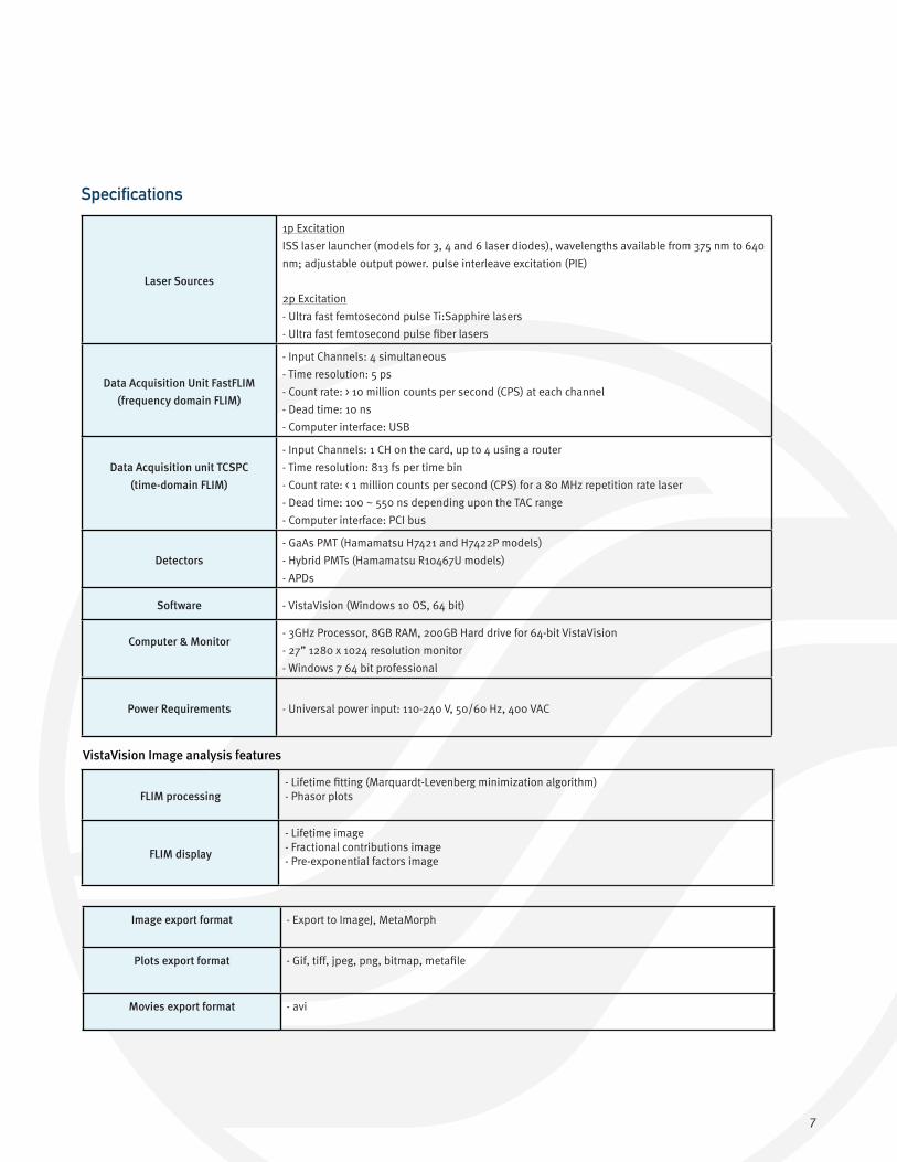
Specifications

Laser Sources

1p Excitation

ISS laser launcher (models for 3, 4 and 6 laser diodes), wavelengths available from 375 nm to 640

nm; adjustable output power. pulse interleave excitation (PIE)

2p Excitation

- Ultra fast femtosecond pulse Ti:Sapphire lasers

- Ultra fast femtosecond pulse fiber lasers

Data Acquisition Unit FastFLIM

(frequency domain FLIM)

- Input Channels: 4 simultaneous

- Time resolution: 5 ps

- Count rate: > 10 million counts per second (CPS) at each channel

- Dead time: 10 ns

- Computer interface: USB

Data Acquisition unit TCSPC

(time-domain FLIM)

- Input Channels: 1 CH on the card, up to 4 using a router

- Time resolution: 813 fs per time bin

- Count rate: < 1 million counts per second (CPS) for a 80 MHz repetition rate laser

- Dead time: 100 ~ 550 ns depending upon the TAC range

- Computer interface: PCI bus

Detectors

- GaAs PMT (Hamamatsu H7421 and H7422P models)

- Hybrid PMTs (Hamamatsu R10467U models)

- APDs

Software - VistaVision (Windows 10 OS, 64 bit)

Computer & Monitor- 3GHz Processor, 8GB RAM, 200GB Hard drive for 64-bit VistaVision

- 27” 1280 x 1024 resolution monitor

- Windows 7 64 bit professional

Power Requirements - Universal power input: 110-240 V, 50/60 Hz, 400 VAC

VistaVision Image analysis features

FLIM processing- Lifetime fitting (Marquardt-Levenberg minimization algorithm)- Phasor plots

FLIM display

- Lifetime image- Fractional contributions image- Pre-exponential factors image

Image export format - Export to ImageJ, MetaMorph

Plots export format - Gif, tiff, jpeg, png, bitmap, metafile

Movies export format - avi

7

For more information please call (217) 359-8681 or visit our website at www.iss.com

Copyright ©2009-2016 ISS, Inc. All Rights Reserved

1602 Newton DriveChampaign, Illinois 61822 USATelephone: (217) 359-8681Telefax: (217) 359-7879Email: iss@iss.com

Statistical function utilized for FFS data analysis

Single set and Global fitting models available in the FFS module

Parameters determined by the FFS module

Autocorrelation (FCS) - One or two species using:

o 2D- or 3D-Gaussian PSF

o 3D-Gaussian-Lorentzian PSF

o one-photon excitation

o two-photon excitation

o presence of flow

- Global analysis fitting

- One or two species using:

o Diffusion coefficient

o Concentration

o Triplet state decay time constant

o Triplet function

o Flow rate

o Size of excitation volume

Photon Counting Histogram (PCH)

Cross-correlation (FCCS)

User Defined Equation

- Up to 50 different user defined equations kept in the panel list for user to choose- Equation could include Sin, Cos, Exponential, etc. Except the integral unclosed form equation- Global analysis fitting

- Up to 30 parameters allowed in the equation

VistaVision FFS analysis features

FastFLIM is covered by US Patent 8,330,123; other patents are pending.

Please email us for specific information on our upgrades packages for Nikon Systems.

8