time response of shape memory alloy actuators
TRANSCRIPT
1
Journal of Intelligent Material Systems and Structures, V.11, Febr.2000, pp.125-134
Time Response of Shape Memory Alloy Actuators
Pavel L. Potapov* and Edson P. da Silva, Technische Universität Berlin, Institute für
Verfahrenstechnik, Salzufer 17/19, D-10587, Berlin, Germany
* Author to whom correspondence should be addressed. Presently with Antwerp University-
RUCA, EMAT, Croenenborgerlaan 171, 2020 Antwerp, Belgium
Key words
shape memory alloy, NiTi, nitinol, flexinol, actuator, time response, convection, transformation
latent heat
Abstract
Force/displacement actuators with the high output power and time response can be fabricated from
shape memory wires or ribbons. Typically Ni-Ti shape memory alloys are used as an active material
in such actuators. They are driven by Joule heating and air convection cooling. In the present work,
the time response of various types of Ni-Ti actuators having different transformation temperatures
and geometrical sizes, is studied systematically under conditions of free and forced air convection
The simple analytical model for calculating the time response is developed which accounts for the
latent heat and thermal hysteresis of transformation. For all the types of considered actuators, the
calculated time response is in a good agreement with that observed experimentally. Finally, on the
base of the suggested model, we present the time response of Ni-Ti actuators calculated as a
function of their transformation temperature and cross section dimensions.
Introduction
2
Linear actuators made from shape memory alloys (SMA) are capable to produce a large actuation
force and/or displacement and can be applied, among others applications, as artificial muscles in
various smart structures. This ability is associated with internal transformations observed in SMA,
most commonly Ni-Ti based alloys. They undergo the diffusionless transformations from the
martensitic (M) to austenitic (A) phase on heating and the A→M transformation on cooling. The
transformations are reversible and can be utilized to convert thermal energy directly into
mechanical work. The dynamic thermomechanical response of shape memory alloys has been
studied experimentally (Leo et al.,1993, Shaw and Kuriakides,1995), however, these authors have
addressed mainly the stress-induced transformations in SMA while practical SMA actuators
normally employ thermally induced phase transformations. A typical method to trigger the
transformations in SMA includes Joule heating for the M→A transition and air convection cooling
for the A→M one. The total time response is composed of the time required for heating up and the
time required for cooling down an actuator. In both the heating and cooling phases, the time
response is strongly controlled by the thermal parameters of SMA and efficiency of the convection
heat exchange between an actuator and surroundings. The dynamic behavior of SMA can be
simulated in the frameworks of constitutive models proposed during last decades. A non-inclusive
list is the theoretical work of Tanaka and Nagaki, 1982, Liang and Roger, 1990, Brinson, 1993,
Likhachev, 1994, Boud and Lagoudas, 1996, Bekker and Brinson, 1997, Seelecke and Müller,
1998, Bo and Lagoudas, 1999. However, in these models, analytical description of the heat transfer
normally neglects the temperature dependence of the SMA heat capacity (Brinson et al, 1996, Liang
and Roger, 1997), while more comprehensive approaches accounting for the latent heat of
transformation need in the complicated numerical algorithms (Bekker et al.,1998, Lagoudas and Bo,
1999).
This paper presents experimental results on impulsive Joule heating and air convection cooling of
several Ni-Ti ribbons and wires having quite different transformation temperatures and geometrical
3
sizes. Due to the small cross-section of the examined ribbons and wires, the heat transfer proceeds
dominantly by convective convection between SMA actuators and surrounding air. The observed
experimental results can be reasonably fitted by the proposed simple analytical model accounting
for the latent heat and thermal hysteresis of transformation. By comparison between the time
responses calculated with different latent heats, it is demonstrated that the effect of the
transformation latent heat cannot be neglected in simulation of the dynamic behavior of SMA. The
proposed model can predict the time response of SMA actuators as a function of their material
parameters and geometrical sizes. Examples of such predictions are given in the last section.
Experimental Procedure and Results
Various types of Ni-Ti ribbons were manufactured by AMT (Herk-de-Stad, Belgium), Raychem
(Menlo Park, California, US) and A.V.Shelyakov (Moscow Engineering Physics Inst., Russia). Ni-
Ti actuator wire (trade mark ”Flexinol 90”) was manufactured by Dynalloy Co. All materials show
approximately the same specific heat capacity of about 0.45mJ/kg/K at room temperature. The
transformation temperatures and latent heat determined by DSC are listed in Table 1 where
actuators are referred as A, R, S, SH and F types depending on their manufacturer. SH ribbons
produced by Shelyakov contained 15 at.% of Hf in order to increase the transformation temperature.
Here, the transformation start and finish temperatures are referred as As and Af for the M→A
transformation and Ms and Mf for the A→M one.
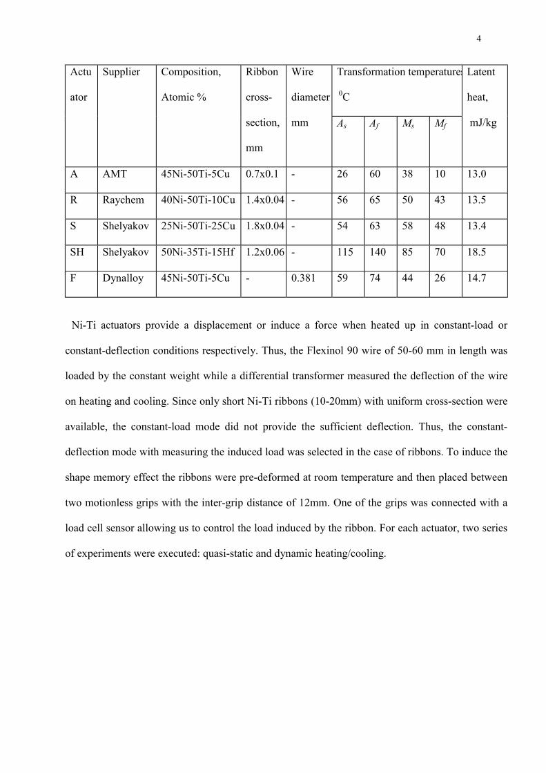
Table 1 Composition, cross section, transformation temperatures and latent heat of Ni-Ti
actuators.
4
Transformation temperatures
0C
Actu
ator
Supplier Composition,
Atomic %
Ribbon
cross-
section,
mm
Wire
diameter
mm As Af Ms Mf
Latent
heat,
mJ/kg
A AMT 45Ni-50Ti-5Cu 0.7x0.1 - 26 60 38 10 13.0
R Raychem 40Ni-50Ti-10Cu 1.4x0.04 - 56 65 50 43 13.5
S Shelyakov 25Ni-50Ti-25Cu 1.8x0.04 - 54 63 58 48 13.4
SH Shelyakov 50Ni-35Ti-15Hf 1.2x0.06 - 115 140 85 70 18.5
F Dynalloy 45Ni-50Ti-5Cu - 0.381 59 74 44 26 14.7
Ni-Ti actuators provide a displacement or induce a force when heated up in constant-load or
constant-deflection conditions respectively. Thus, the Flexinol 90 wire of 50-60 mm in length was
loaded by the constant weight while a differential transformer measured the deflection of the wire
on heating and cooling. Since only short Ni-Ti ribbons (10-20mm) with uniform cross-section were
available, the constant-load mode did not provide the sufficient deflection. Thus, the constant-
deflection mode with measuring the induced load was selected in the case of ribbons. To induce the
shape memory effect the ribbons were pre-deformed at room temperature and then placed between
two motionless grips with the inter-grip distance of 12mm. One of the grips was connected with a
load cell sensor allowing us to control the load induced by the ribbon. For each actuator, two series
of experiments were executed: quasi-static and dynamic heating/cooling.
5
0
2
4
6
8
10
12
14
16
18
20
20 30 40 50 60 70 80 90 100Temperature (0C)
Load
(N)
experimentalapproximated
A-ribbon
S-ribbon
0
1
2
3
4
5
6
7
8
9
10
20 40 60 80 100 120 140Temperature (0C)
Load
(N)
experimentalapproximated
R-ribbon
SH-ribbon
M-M transition
(a) (b)
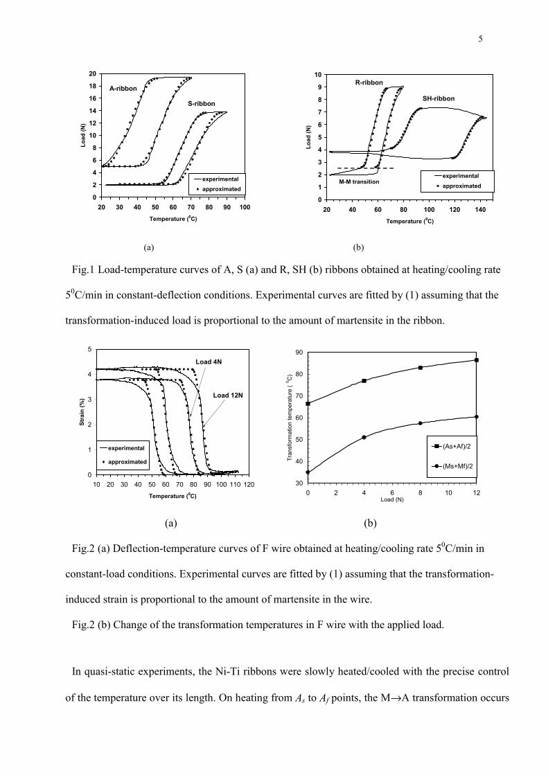
Fig.1 Load-temperature curves of A, S (a) and R, SH (b) ribbons obtained at heating/cooling rate
50C/min in constant-deflection conditions. Experimental curves are fitted by (1) assuming that the
transformation-induced load is proportional to the amount of martensite in the ribbon.
0
1
2
3
4
5
10 20 30 40 50 60 70 80 90 100 110 120
Temperature (0C)
Stra
in (%
)
experimental
approximated
Load 4N
Load 12N
30
40
50
60
70
80
90
0 2 4 6 8 10 12Load (N)
Tran
sfor
mat
ion
tem
pera
ture
( 0 C
)
(As+Af)/2
(Ms+Mf)/2
(a) (b)
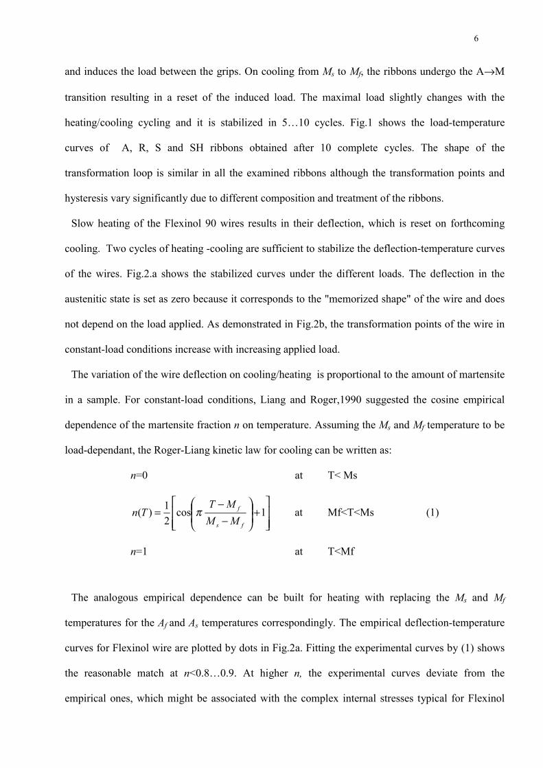
Fig.2 (a) Deflection-temperature curves of F wire obtained at heating/cooling rate 50C/min in
constant-load conditions. Experimental curves are fitted by (1) assuming that the transformation-
induced strain is proportional to the amount of martensite in the wire.
Fig.2 (b) Change of the transformation temperatures in F wire with the applied load.
In quasi-static experiments, the Ni-Ti ribbons were slowly heated/cooled with the precise control
of the temperature over its length. On heating from As to Af points, the M→A transformation occurs
6
and induces the load between the grips. On cooling from Ms to Mf, the ribbons undergo the A→M
transition resulting in a reset of the induced load. The maximal load slightly changes with the
heating/cooling cycling and it is stabilized in 5…10 cycles. Fig.1 shows the load-temperature
curves of A, R, S and SH ribbons obtained after 10 complete cycles. The shape of the
transformation loop is similar in all the examined ribbons although the transformation points and
hysteresis vary significantly due to different composition and treatment of the ribbons.
Slow heating of the Flexinol 90 wires results in their deflection, which is reset on forthcoming
cooling. Two cycles of heating -cooling are sufficient to stabilize the deflection-temperature curves
of the wires. Fig.2.a shows the stabilized curves under the different loads. The deflection in the
austenitic state is set as zero because it corresponds to the "memorized shape" of the wire and does
not depend on the load applied. As demonstrated in Fig.2b, the transformation points of the wire in
constant-load conditions increase with increasing applied load.
The variation of the wire deflection on cooling/heating is proportional to the amount of martensite
in a sample. For constant-load conditions, Liang and Roger,1990 suggested the cosine empirical
dependence of the martensite fraction n on temperature. Assuming the Ms and Mf temperature to be
load-dependant, the Roger-Liang kinetic law for cooling can be written as:
n=0 at T< Ms
+
−
−= 1cos
21)(
fs
f
MMMT
Tn π at Mf<T<Ms (1)
n=1 at T<Mf
The analogous empirical dependence can be built for heating with replacing the Ms and Mf
temperatures for the Af and As temperatures correspondingly. The empirical deflection-temperature
curves for Flexinol wire are plotted by dots in Fig.2a. Fitting the experimental curves by (1) shows
the reasonable match at n<0.8…0.9. At higher n, the experimental curves deviate from the
empirical ones, which might be associated with the complex internal stresses typical for Flexinol
7
wire. In the case of Ni-Ti ribbons, the coupling between the induced load and the martensite
fraction results in an increase of transformation temperatures, especially for Af and Ms points.
Indeed, the comparison of the curves in Fig 1 with the data in Table 1 reveals an increase of all the
transformation points and the transformation ranges (Af-As) and (Ms-Mf). However, Fig.1
demonstrates that the empirical dependence (1) with the modified Ms , Mf , Af and As parameters can
be still used to build the load-temperature curves in constant-deflection conditions. In this case, Ms ,
Mf , Af and As temperatures should be calculated from the well-known Clausius-Clapeiron equation
or taken from experiments. Out of the transformation range, some ribbons show the small negative
slope of the load-temperature curves due to thermal expansion. The R ribbons indicate the more
complex behavior with a positive slope of the load below Mf temperature. Moreover, a positive
slope is observed even on cooling far below room temperature. That is a result of the transition
between different types of martensite reported in a NiTi-10%Cu alloy, which was the material of
the R ribbons. In this paper, we neglect the martensite→martensite transition because it is
associated with the much smaller latent heat and induced load than the A→M one.
0
2
4
6
8
10
12
14
16
18
20
-4 -2 0 2 4 6 8 10 12time (s)
Load
(N)
set: 700C
90% reset: 260C
tH=0.5s
tH=3s
tH=0.1s
A
0
1
2
3
4
5
6
7
8
9
-3 -2 -1 0 1 2 3time (s)
Load
(N)
set: 800C
90% reset: 510C
tH=2s
tH=6s
tH=0.5s
R
(a) (b)
8
0
2
4
6
8
10
12
14
-3 -2 -1 0 1 2 3time (s)
Load
(N)
set: 900C
90% reset: 570C
tH=0.5s
tH=3s
tH=0.1s
S
3
4
5
6
7
8
-3 -2 -1 0 1 2 3time (s)
Load
(N)
set: 1400C
90% reset: 750C
tH=0.5s
tH=3s
tH=0.1s
SH
(c) (d)
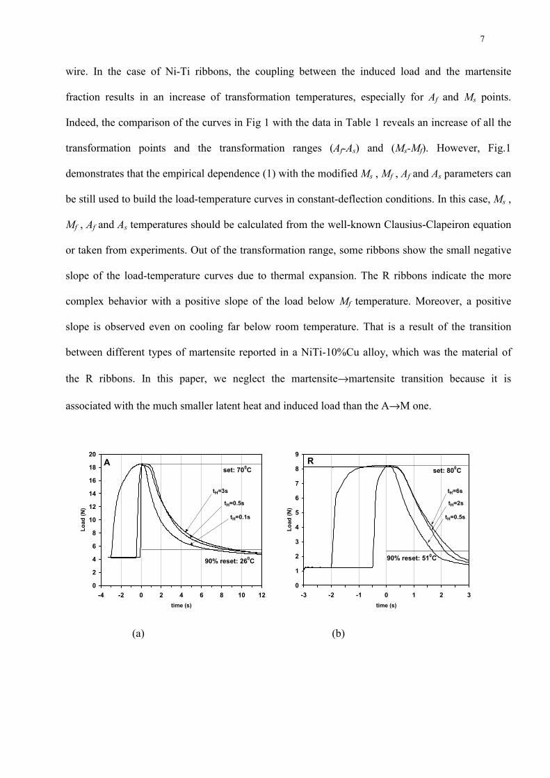
Fig.3 Impulsive Joule heating of A(a), R (b), S (c) and SH (d) ribbons followed by free air
convection cooling. The duration of impulse is denoted by tH. For convenience, each curve is
shifted along the time-axis such as cooling starts always at t=0 regardless of the heating duration.
-0.5
0
0.5
1
1.5
2
2.5
3
-4 -2 0 2 4 6 8 10 12time (s)
Def
lect
ion
(mm
)
set: 890C
90% reset: 540C
tH=0.5stH=2s
tH=0.1s
tH=6s
F6
-0.5
0
0.5
1
1.5
2
2.5
3
-4 -2 0 2 4 6 8 10 12time (s)
Def
lect
ion
(mm
)
set: 950C
90% reset: 600C
tH=0.5s
tH=2s
tH=0.1s
tH=6s
F12
(a) (b)
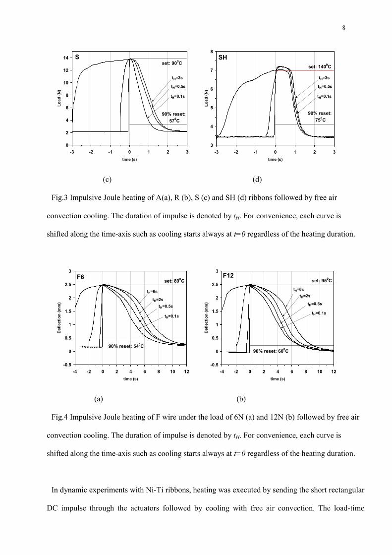
Fig.4 Impulsive Joule heating of F wire under the load of 6N (a) and 12N (b) followed by free air
convection cooling. The duration of impulse is denoted by tH. For convenience, each curve is
shifted along the time-axis such as cooling starts always at t=0 regardless of the heating duration.
In dynamic experiments with Ni-Ti ribbons, heating was executed by sending the short rectangular
DC impulse through the actuators followed by cooling with free air convection. The load-time
9
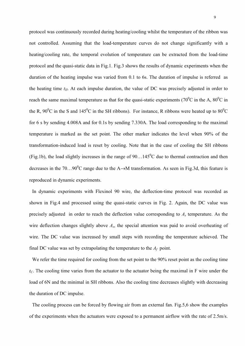
protocol was continuously recorded during heating/cooling whilst the temperature of the ribbon was
not controlled. Assuming that the load-temperature curves do not change significantly with a
heating/cooling rate, the temporal evolution of temperature can be extracted from the load-time
protocol and the quasi-static data in Fig.1. Fig.3 shows the results of dynamic experiments when the
duration of the heating impulse was varied from 0.1 to 6s. The duration of impulse is referred as
the heating time tH. At each impulse duration, the value of DC was precisely adjusted in order to
reach the same maximal temperature as that for the quasi-static experiments (700C in the A, 800C in
the R, 900C in the S and 1450C in the SH ribbons). For instance, R ribbons were heated up to 800C
for 6 s by sending 4.008A and for 0.1s by sending 7.330A. The load corresponding to the maximal
temperature is marked as the set point. The other marker indicates the level when 90% of the
transformation-induced load is reset by cooling. Note that in the case of cooling the SH ribbons
(Fig.1b), the load slightly increases in the range of 90…1450C due to thermal contraction and then
decreases in the 70…900C range due to the A→M transformation. As seen in Fig.3d, this feature is
reproduced in dynamic experiments.
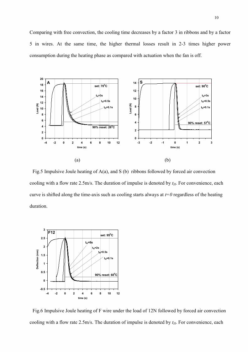
In dynamic experiments with Flexinol 90 wire, the deflection-time protocol was recorded as
shown in Fig.4 and processed using the quasi-static curves in Fig. 2. Again, the DC value was
precisely adjusted in order to reach the deflection value corresponding to As temperature. As the
wire deflection changes slightly above As, the special attention was paid to avoid overheating of
wire. The DC value was increased by small steps with recording the temperature achieved. The
final DC value was set by extrapolating the temperature to the Af point.
We refer the time required for cooling from the set point to the 90% reset point as the cooling time
tC. The cooling time varies from the actuator to the actuator being the maximal in F wire under the
load of 6N and the minimal in SH ribbons. Also the cooling time decreases slightly with decreasing
the duration of DC impulse.
The cooling process can be forced by flowing air from an external fan. Fig.5,6 show the examples
of the experiments when the actuators were exposed to a permanent airflow with the rate of 2.5m/s.
10
Comparing with free convection, the cooling time decreases by a factor 3 in ribbons and by a factor
5 in wires. At the same time, the higher thermal losses result in 2-3 times higher power
consumption during the heating phase as compared with actuation when the fan is off.
0
2
4
6
8
10
12
14
16
18
20
-4 -2 0 2 4 6 8 10 12time (s)
Load
(N)
set: 700C
90% reset: 260C
tH=0.5s
tH=3s
tH=0.1s
A
0
2
4
6
8
10
12
14
-3 -2 -1 0 1 2 3time (s)
Load
(N)
set: 900C
90% reset: 570C
tH=0.5s
tH=3s
tH=0.1s
S
(a) (b)
Fig.5 Impulsive Joule heating of A(a), and S (b) ribbons followed by forced air convection
cooling with a flow rate 2.5m/s. The duration of impulse is denoted by tH. For convenience, each
curve is shifted along the time-axis such as cooling starts always at t=0 regardless of the heating
duration.
-0.5
0
0.5
1
1.5
2
2.5
3
-4 -2 0 2 4 6 8 10 12time (s)
Def
lect
ion
(mm
)
set: 950C
90% reset: 600C
tH=0.5stH=2s
tH=0.1s
tH=6s
F12
Fig.6 Impulsive Joule heating of F wire under the load of 12N followed by forced air convection
cooling with a flow rate 2.5m/s. The duration of impulse is denoted by tH. For convenience, each
11
curve is shifted along the time-axis such as cooling starts always at t=0 regardless of the heating
duration.
Modeling
The existing models can successfully simulate the dynamic behavior of SMA using numerical
algorithms (Bekker et al, 1998, Lagoudas and Bo, 1999). In contrast, in this section, we will
develop the simple model suitable for the easy analytical prediction of the time response of SMA
actuators. Similar analytical modeling has been suggested by Brailovski et al., 1996. They,
however, employed the polynomial kinetic law, which needs a number of experimentally
determined coefficients. In this paper, for the cooling process, we will utilize the Liang-Roger
kinetic law (1) that depends on only the parameters Ms and Mf. The same equation can be applied
for the heating process with replacing the Ms and Mf temperatures for the Af = Ms+∆T and
As=Mf+∆T temperatures correspondingly, where ∆T is the thermal hysteresis of transformation.
Although during actuation the heating phase precedes the cooling one, we shall consider firstly the
cooling phase, which is easier to model.
Cooling Phase
During the cooling phase, a Ni-Ti actuator should be cooled down from the Af temperature. If we
assume that a single temperature characterizes the temperature of an actuator and neglect heat
conduction at the actuator ends, the heat transfer problem is defined by
( ) ( )dtTThFHdndTcV p 0−=∆+− ρ at Ms<T<Af (2)
where ρ is the density of Ni-Ti (about 6500 kg/m3), cp is the Ni-Ti specific heat capacity in the
absence of transformations, V and F are the volume and the free surface of an actuator respectively,
12
∆H is the integral latent heat for transformation on cooling, h is the coefficient of the heat exchange
between an actuator and surroundings, T is the temperature of a Ni-Ti actuator and T0 is the
temperature of surroundings. Introducing, after Wirtz et al., 1995, dimensionless variables
fs
f
MMMT
T−
−=´ t
VchFtp ρ
=´ (dimensionless time),
fs
f
MMTM
S−−
= 0 ( dimensionless difference between the transformation and room temperatures),
)( fsp MMVcHH
−∆=
ρ (dimensionless transformation latent heat)
and fs
sf
fs MMMA
MMTG
−−
=−
∆= (dimensionless transformation hysteresis) and assuming that that
the martensite volume fraction depends on temperature as (1), the Eq.(2) is rewritten as
STdtdT +=− ´
´´ at 1<T´<1+G and at T´<0 (3)
STdtdTTH +=
+− ´
´´´)sin(
21 ππ at 0<T’<1 (4)
Integrating (3) with the boundary condition T'=1+G at t'=0 we obtain the simplest temperature-time
curve:
( ) )1ln(´ln´ SGSTt ++++−= at 1<T´<1+G (5)
In the regime 0<T’<1, integration of (4) with the boundary condition T'=1 at t'=t'1=-
ln(1+S)+ln(1+G+S) gives the solution
( )( ) ( )( ) ( )[ ] ( ) ( )( ) ( )( )[ ]{ }SCiSTCiSSSiSTSiSH
SSTtt
+−+−+−+
−+++−=
1´sin1(´cos2
)1ln(´ln´´ 1
πππππππ at 0<T’<1 (6)
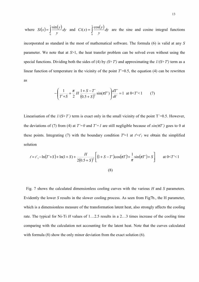
13
where ( ) ( )∫=x
dyy
yxSi0
sin and ( )∫=x
dyy
yxCi0
cos)( are the sine and cosine integral functions
incorporated as standard in the most of mathematical software. The formula (6) is valid at any S
parameter. We note that at S>1, the heat transfer problem can be solved even without using the
special functions. Dividing both the sides of (4) by (S+T') and approximating the 1/(S+T') term as a
linear function of temperature in the vicinity of the point T´=0.5, the equation (4) can be rewritten
as
( ) 1´´´)sin(
5.0´1
2´1
2 =
+−++
+−
dtdTT
STSH
STππ at 0<T’<1 (7)
Linearisation of the 1/(S+T´) term is exact only in the small vicinity of the point T´=0.5. However,
the deviations of (7) from (4) at T´=0 and T´=1 are still negligible because of sin(πT´) goes to 0 at
these points. Integrating (7) with the boundary condition T'=1 at t'=t'1 we obtain the simplified
solution
( )( )
( ) ( ) ( )
++−+
+++++−= STTTS
SHSSTtt ´sin1´cos´15.02
)1ln(´ln´´ 21 ππ
π at 0<T’<1
(8)
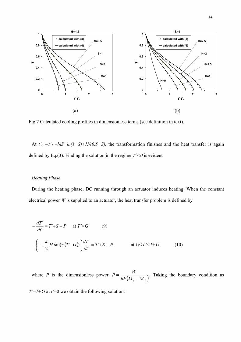
Fig. 7 shows the calculated dimensionless cooling curves with the various H and S parameters.
Evidently the lower S results in the slower cooling process. As seen from Fig7b., the H parameter,
which is a dimensionless measure of the transformation latent heat, also strongly affects the cooling
rate. The typical for Ni-Ti H values of 1…2.5 results in a 2…3 times increase of the cooling time
comparing with the calculation not accounting for the latent heat. Note that the curves calculated
with formula (8) show the only minor deviation from the exact solution (6).
14
0
0.2
0.4
0.6
0.8
1
0 1 2 3t´-t´1
T´
calculated with (8)
calculated with (6)S=0.5
S=1
S=2
S=3
H=1.5
0
0.2
0.4
0.6
0.8
1
0 1 2 3t´-t´1
T´
calculated with (8)
calculated with (6)H=2.5
H=2
H=1.5
H=1H=0
S=1
(a) (b)
Fig.7 Calculated cooling profiles in dimensionless terms (see definition in text).
At t’0 =t’1 –lnS+ln(1+S)+H/(0.5+S), the transformation finishes and the heat transfer is again
defined by Eq.(3). Finding the solution in the regime T´<0 is evident.
Heating Phase
During the heating phase, DC running through an actuator induces heating. When the constant
electrical power W is supplied to an actuator, the heat transfer problem is defined by
PSTdtdT −+=− ´
´´ at T’<G (9)
( ) PSTdtdTGTH −+=
−+− ´
´´)´sin(
21 ππ at G<T’<1+G (10)
where P is the dimensionless power ( )fs MMhFWP
−= . Taking the boundary condition as
T’=1+G at t’=0 we obtain the following solution:
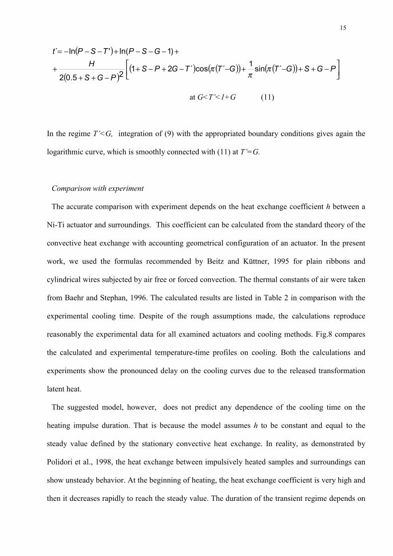
15
( )
( )( ) ( )( ) ( )( )
−++−+−−+−+
−+++
+−−−+−−−=
PGSGTGTTGPSPGS
HGSPTSPt
´sin1´cos´2125.02
)1ln('ln´
ππ
π
at G<T’<1+G (11)
In the regime T’<G, integration of (9) with the appropriated boundary conditions gives again the
logarithmic curve, which is smoothly connected with (11) at T’=G.
Comparison with experiment
The accurate comparison with experiment depends on the heat exchange coefficient h between a
Ni-Ti actuator and surroundings. This coefficient can be calculated from the standard theory of the
convective heat exchange with accounting geometrical configuration of an actuator. In the present
work, we used the formulas recommended by Beitz and Küttner, 1995 for plain ribbons and
cylindrical wires subjected by air free or forced convection. The thermal constants of air were taken
from Baehr and Stephan, 1996. The calculated results are listed in Table 2 in comparison with the
experimental cooling time. Despite of the rough assumptions made, the calculations reproduce
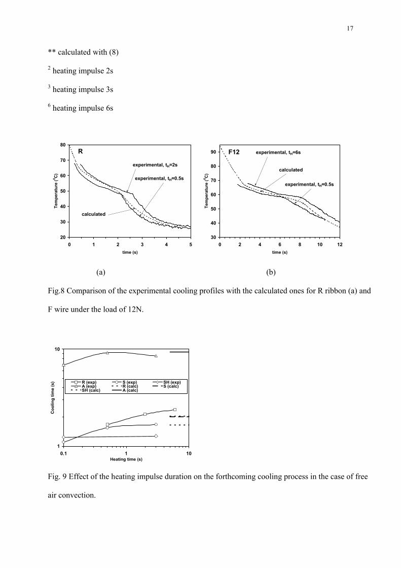
reasonably the experimental data for all examined actuators and cooling methods. Fig.8 compares
the calculated and experimental temperature-time profiles on cooling. Both the calculations and
experiments show the pronounced delay on the cooling curves due to the released transformation
latent heat.
The suggested model, however, does not predict any dependence of the cooling time on the
heating impulse duration. That is because the model assumes h to be constant and equal to the
steady value defined by the stationary convective heat exchange. In reality, as demonstrated by
Polidori et al., 1998, the heat exchange between impulsively heated samples and surroundings can
show unsteady behavior. At the beginning of heating, the heat exchange coefficient is very high and
then it decreases rapidly to reach the steady value. The duration of the transient regime depends on
16
geometry of a sample and properties of surrounding fluid. For actuators examined in the present
work, the transient regime takes approximately 2 s. That can be concluded from the analysis of the
heating branches of the load (deflection) curves in Fig. 3 and 4. The load (deflection) reaches the
steady level in approximately 2 s after switching DC on. In the case of the 0.1 and 0.5s impulses,
the current is cut before the stationary conditions are reached, thus, further cooling proceeds under
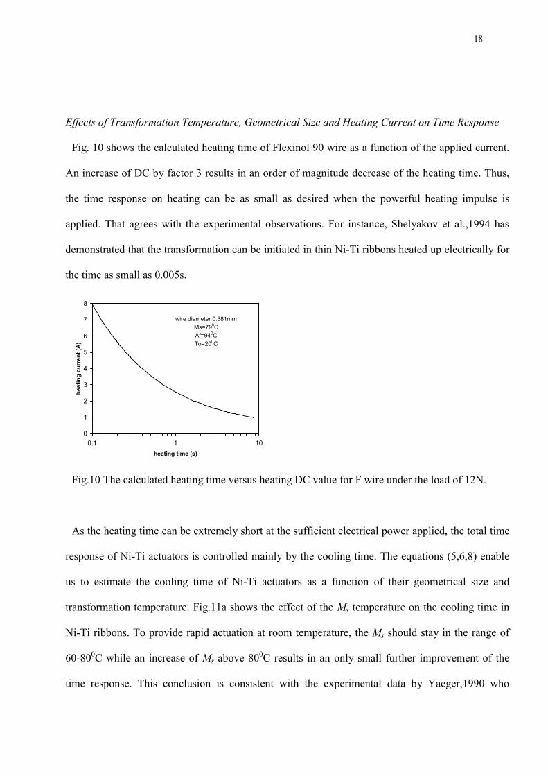
conditions of the unsteady heat exchange with the increased heat exchange coefficient. Fig.9
demonstrates the effect of the heating impulse duration on the forthcoming cooling process. The
cooling time firstly increases with the heating time and then comes to saturation at tH=2…6s. These
saturation values can be adequately modeled in terms of stationary heat exchange as demonstrated
above. The modeling of the shorter heating impulses (0.1…0.5s) should however address the
unsteady heat transfer problem, which can not be solved analytically.
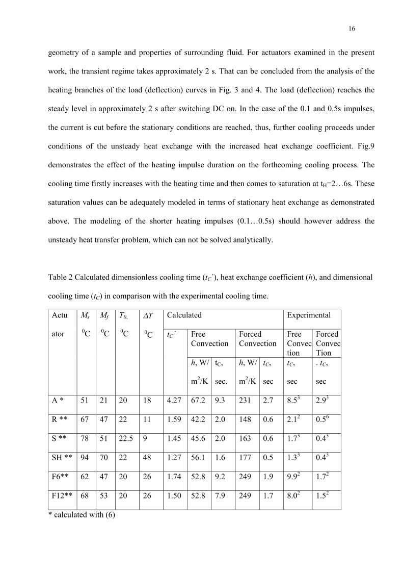
Table 2 Calculated dimensionless cooling time (tC´), heat exchange coefficient (h), and dimensional
cooling time (tC) in comparison with the experimental cooling time.
Calculated Experimental
FreeConvection
ForcedConvection
FreeConvection
ForcedConvecTion
Actu
ator
Ms
0C
Mf
0C
T0,
0C
∆T
0C tC´
h, W/
m2/K
tC,
sec.
h, W/
m2/K
tC,
sec
tC,
sec
. tC,
sec
A * 51 21 20 18 4.27 67.2 9.3 231 2.7 8.53 2.93
R ** 67 47 22 11 1.59 42.2 2.0 148 0.6 2.12 0.56
S ** 78 51 22.5 9 1.45 45.6 2.0 163 0.6 1.73 0.43
SH ** 94 70 22 48 1.27 56.1 1.6 177 0.5 1.33 0.43
F6** 62 47 20 26 1.74 52.8 9.2 249 1.9 9.92 1.72
F12** 68 53 20 26 1.50 52.8 7.9 249 1.7 8.02 1.52
* calculated with (6)
17
** calculated with (8)
2 heating impulse 2s
3 heating impulse 3s
6 heating impulse 6s
20
30
40
50
60
70
80
0 1 2 3 4 5time (s)
Tem
pera
ture
(0 C)
calculated
experimental, tH=2s
experimental, tH=0.5s
R
30
40
50
60
70
80
90
0 2 4 6 8 10 12time (s)
Tem
pera
ture
(0 C)
calculated
experimental, tH=6s
experimental, tH=0.5s
F12
(a) (b)
Fig.8 Comparison of the experimental cooling profiles with the calculated ones for R ribbon (a) and
F wire under the load of 12N.
1
10
0.1 1 10Heating time (s)
Coo
ling
time
(s) R (exp) S (exp) SH (exp)
A (exp) R (calc) S (calc)SH (calc) A (calc)
Fig. 9 Effect of the heating impulse duration on the forthcoming cooling process in the case of free
air convection.
18
Effects of Transformation Temperature, Geometrical Size and Heating Current on Time Response
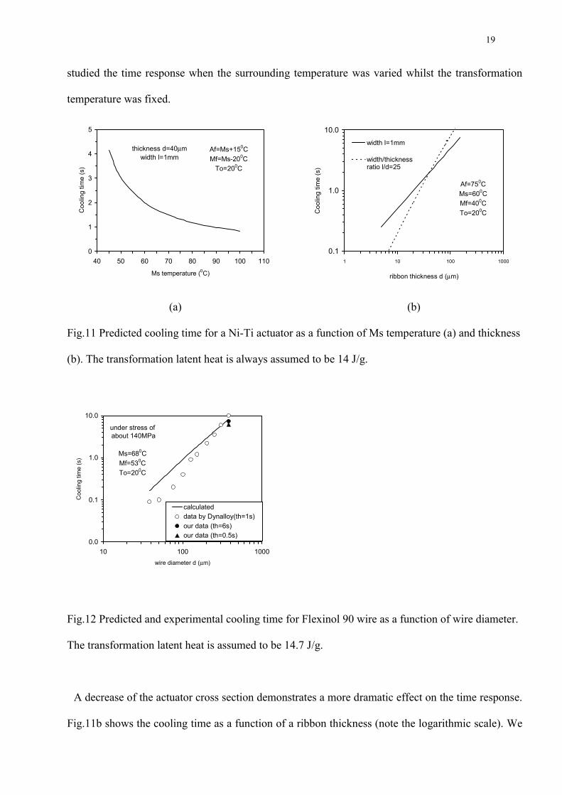
Fig. 10 shows the calculated heating time of Flexinol 90 wire as a function of the applied current.
An increase of DC by factor 3 results in an order of magnitude decrease of the heating time. Thus,
the time response on heating can be as small as desired when the powerful heating impulse is
applied. That agrees with the experimental observations. For instance, Shelyakov et al.,1994 has
demonstrated that the transformation can be initiated in thin Ni-Ti ribbons heated up electrically for
the time as small as 0.005s.
0
1
2
3
4
5
6
7
8
0.1 1 10heating time (s)
heat
ing
curr
ent (
A)
wire diameter 0.381mmMs=790CAf=940CTo=200C
Fig.10 The calculated heating time versus heating DC value for F wire under the load of 12N.
As the heating time can be extremely short at the sufficient electrical power applied, the total time
response of Ni-Ti actuators is controlled mainly by the cooling time. The equations (5,6,8) enable
us to estimate the cooling time of Ni-Ti actuators as a function of their geometrical size and
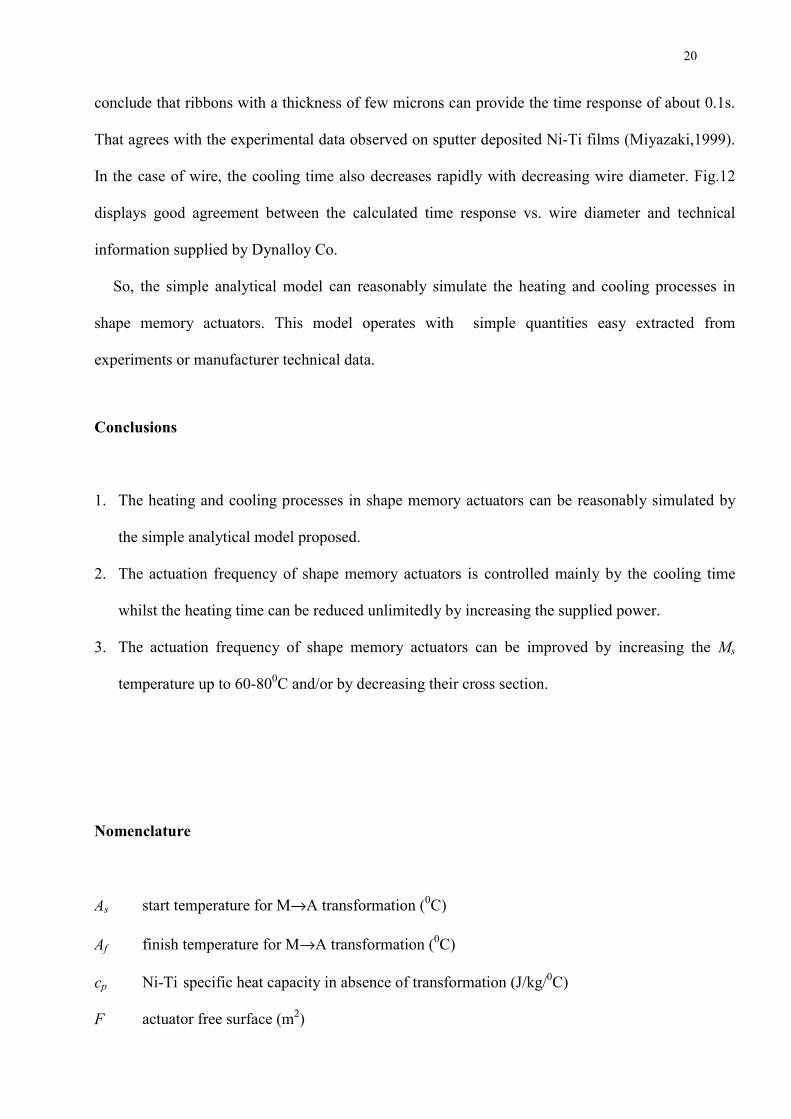
transformation temperature. Fig.11a shows the effect of the Ms temperature on the cooling time in
Ni-Ti ribbons. To provide rapid actuation at room temperature, the Ms should stay in the range of
60-800C while an increase of Ms above 800C results in an only small further improvement of the
time response. This conclusion is consistent with the experimental data by Yaeger,1990 who
19
studied the time response when the surrounding temperature was varied whilst the transformation
temperature was fixed.
0
1
2
3
4
5
40 50 60 70 80 90 100 110
Ms temperature (0C)
Coo
ling
time
(s)
thickness d=40µmwidth l=1mm
Af=Ms+150CMf=Ms-200C
To=200C
0.1
1.0
10.0
1 10 100 1000
ribbon thickness d (µm)
Coo
ling
time
(s)
width l=1mm
width/thicknessratio l/d=25
Af=750CMs=600CMf=400CTo=200C
(a) (b)
Fig.11 Predicted cooling time for a Ni-Ti actuator as a function of Ms temperature (a) and thickness
(b). The transformation latent heat is always assumed to be 14 J/g.
0.0
0.1
1.0
10.0
10 100 1000wire diameter d (µm)
Coo
ling
time
(s)
calculateddata by Dynalloy(th=1s) our data (th=6s)our data (th=0.5s)
under stress of about 140MPa
Ms=680CMf=530CTo=200C
Fig.12 Predicted and experimental cooling time for Flexinol 90 wire as a function of wire diameter.
The transformation latent heat is assumed to be 14.7 J/g.
A decrease of the actuator cross section demonstrates a more dramatic effect on the time response.
Fig.11b shows the cooling time as a function of a ribbon thickness (note the logarithmic scale). We
20
conclude that ribbons with a thickness of few microns can provide the time response of about 0.1s.
That agrees with the experimental data observed on sputter deposited Ni-Ti films (Miyazaki,1999).
In the case of wire, the cooling time also decreases rapidly with decreasing wire diameter. Fig.12
displays good agreement between the calculated time response vs. wire diameter and technical
information supplied by Dynalloy Co.
So, the simple analytical model can reasonably simulate the heating and cooling processes in
shape memory actuators. This model operates with simple quantities easy extracted from
experiments or manufacturer technical data.
Conclusions
1. The heating and cooling processes in shape memory actuators can be reasonably simulated by
the simple analytical model proposed.
2. The actuation frequency of shape memory actuators is controlled mainly by the cooling time
whilst the heating time can be reduced unlimitedly by increasing the supplied power.
3. The actuation frequency of shape memory actuators can be improved by increasing the Ms
temperature up to 60-800C and/or by decreasing their cross section.
Nomenclature
As start temperature for M→A transformation (0C)
Af finish temperature for M→A transformation (0C)
cp Ni-Ti specific heat capacity in absence of transformation (J/kg/0C)
F actuator free surface (m2)
21
G dimensionless hysteresis of transformation
H dimensionless integral latent heat of transformation
∆H integral latent heat of transformation (J/kg)
h coefficient of heat exchange between an actuator and surroundings (m2/K)
Ms start temperature for the A→M transformation (0C)
Mf finish temperature for the A→M transformation (0C)
n volume fracture of martensite
P dimensionless electric power supplied to an actuator
S dimensionless parameter indicating the difference between transformation and room
temperatures
SMA shape memory alloys
T temperature of an actuator (0C)
T0 surroundings temperature (0C)
T' dimensionless temperature of an actuator
t time (s)
tH heating time, i.e. the time required for heating of an actuator from T0 to Af (s)
tC cooling time, i.e. the time required for cooling of an actuator from Af to the temperature at
which 90% of the induced deflection ( or load) is reset (s)
t' dimensionless time
t'0 dimensionless time at which T' reaches 0 on cooling
W electrical power supplied to actuator (W)
∆T thermal hysteresis of transformation
ρ density of Ni-Ti (kg/m3)
22
Acknowledgements
The stay of authors in Germany was supported by Alexander von Humboldt-Stiftung (PLP) and
Deutscher Akademischer Austauschdienst (EPDS). The authors would like to thank Dr.
A.V.Shelyakov for providing ribbons and consultations. The authors acknowledge discussions with
Prof. I.Müller and other members of the Thermodynamik team in Technische Universität Berlin.
References
• Baehr H.D. and Stephan K.. 1996."Wärme-und Stoffübertragung", Springer-Verlag, Berlin.
• Beitz W. and Küttner K.H.. 1995. "Dubbel Tashenbuch für den maschinenbau", Springer-
Verlag, Berlin.
• Bekker A. and Brinson L.C. 1997. "Temperatire-induced phase transformation in a shape
memory alloy: phase diagram based kinetics approach", J. Mech. Solids, 45, pp.949-988.
• Bekker A., Brinson L.C. and Issen K. 1998. "Localized and diffuse thermoinduced phase
transformation in 1-D shape memory alloys", J. of Intell. Mat. Syst.&Struct., 9, pp.355-365.
• Bo Z., LagoudasD.C. and Miller D. 1999."Material characterization of SMA actuators under
nonproportional thermomechanical loading", J. of Eng. Mat. &Tech., 121, pp.75-85.
• Boud J.G. and Lagoudas D.C. 1996."A thermodynamic constitutive model for the shape
memory materials. Part I: The monolithic shape memory alloys", Int. J. of Plasticity, 12,
pp.805-842.
• Brailovski V., Trochu F. and Daigneault G. 1996."Themporal characteristics of shape memory
linear actuators and application to circuit breakers", Mat.&Design, 17, pp.151-158.
23
• Brinson L.C. 1993. "One dimensional constitutive behavior of shape memory aloys", J. of Intell.
Mat. Syst.&Struct., 4(2), pp.229-249.
• Brinson L.C., Bekker A. and Hwang S. 1996. "Deformation of shape memory alloys due to
thermo-induced transformation", J. of Intell. Mat. Syst.&Struct., 7, pp.97-107.
• Lagoudas D.C. and Bo Z. 1999. "Thermomechanical modeling of polycrystalline SMAs under
cyclic loading, Part II: Material characterization and experimental results for a specific
transformation cycle", Int. J. of Eng. Sci., 37, pp.1141-1174.
• Leo P.H.; Shield T.W. and Bruno O.P. 1993."Transient heat transfer effects on the pseudoelastic
behavior of shape-memory wires", Acta Metall. Mater., 41, pp.2477-2485.
• Liang C. and Roger C.A. 1990. "One-dimensional thermomechanical constitutive relations for
shape memory materials", J. of Intell. Mat. Syst.&Struct., 1(2), pp.207-234.
• Liang C. and Roger C.A. 1997."Design of shape memory alloys", J. of Intell. Mat.
Syst.&Struct., 8, pp.303-313.
• Likhachev V.A. 1994. "Theory of functional and mechanical properties of materials undergoing
reversible martensitic tranformations", Physics of Metals &Metallography, 77, pp.120-133.
• Miyazaki S. 1999. "Ni-Ti SMA thin films and their applications", 1st European Conf. on Shape
Memory and Superelastic Technologies, Antwerp, Belgium , in press.
• Polidori G., Lachi M. and Pader J. 1998. "Unsteady convective heat transfer on a semi-infinite
flat surface impulsively heated", Int. Comm. Heat Mass Transfer, 25, pp.33-42.
• Seelecke S. and Müller I. 1998. "Thermodynamic aspects of shape memory alloys in "Shape
memory alloys - from microstructure to macroscopic properties", Airoldi, G. (ed.), TransTech
Publ., Zürich,
• Shaw J.A. and Kuriakides S. 1995. "Thermomechanical aspects of NiTi", J. Mech. Phys. Solids,
43, pp.1243-1281.
24
• Shelyakov A.V., Antonov V.A., Bukovsky Yu.A. and Matveeva N.M.. 1994. "Optical devices
based on shape memory effect for signal processing", Proc. 1st Int. Conf. on Shape Memory and
Superelastic Technologies, Pasific Grove, California, USA, pp.335-340.
• Tanaka Y. and Nagaki S. 1982. "A tharmomechanical description of materials with internal
variables in the process of phase transitions", Ingenier Archiv., 51, pp.287-299.
• Wirtz R.A., Gordaninejad F. and Wu W. 1995. "Free response of a thermally driven, composite
actuator", J. Intell. Mat. Systems and Structures, 5, pp.364-371.
• Yaeger J.R. 1990. "Electrical actuators: alloy selection, processing and evaluation" in
"Engineering Aspects of Shape Memory Alloys", ed. T.W.Duerig et al., Butterworth-
Heinemann, London, pp.219-233.