time frequency analysis – an application to fmcw … · time frequency analysis – an...

The University of KansasDepartment of Electrical Engineering and Computer Science

TIME FREQUENCY ANALYSIS – An Application to FMCW Radars

BALAJI NAGARAJANMaster’s Project Defense

January 27, 2004

Committee:Dr. Glenn Prescott (Chair)

Dr. Christopher AllenDr. Swapan Chakrabarti


OUTLINE Introduction

What is Joint Time – Frequency analysis ? Application of JTFA to radar signal processing

Background FMCW (sea-ice) radar system design & specifications Need for Time – Frequency analysis of radar range profiles

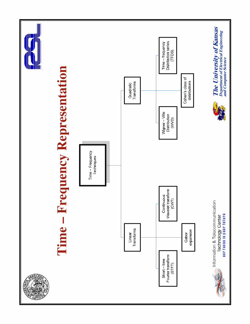
Time – Frequency Representation Different techniques – classification & description

Experiments and Results Ideal simulations Sea-ice radar testing

Conclusions & Future Work


What is Joint Time – Frequency Analysis ? Fourier Analysis

Signal – superposition of weighted sinusoidal functions

Frequency attributes are exactly described

Joint Time – Frequency transforms Characterize behavior of time-varying

frequency content of signal Powerful tool for removing noise &

interference

Drawbacks Inability to express signals whose

frequency contents change over time Examples – speech & music


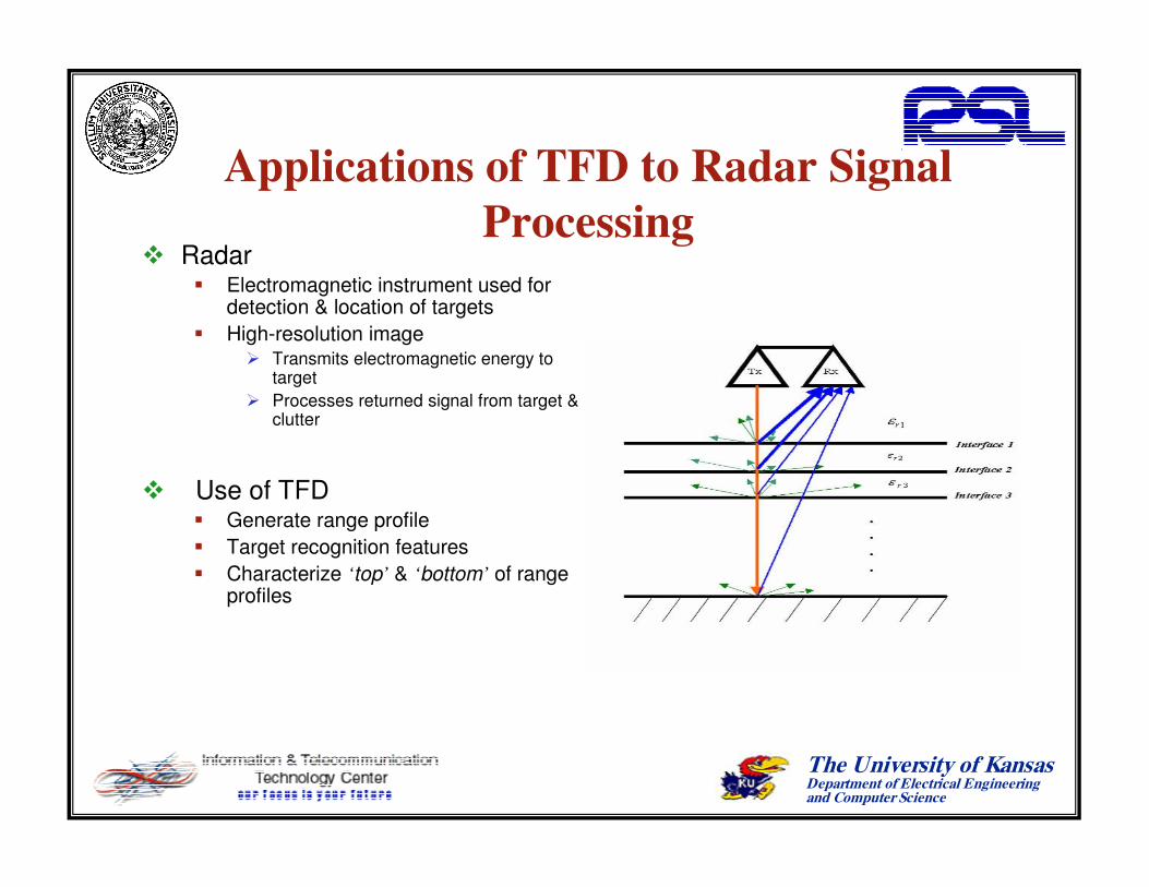
Applications of TFD to Radar Signal Processing

Radar Electromagnetic instrument used for

detection & location of targets High-resolution image

¾ Transmits electromagnetic energy to target

¾ Processes returned signal from target & clutter

Use of TFD Generate range profile Target recognition features Characterize ‘top’ & ‘bottom’ of range

profiles


FMCW Radar Design Background

Measurement of sea-ice thickness VHF pulse radars did not have sufficient range resolution

Frequency Modulated Continuous Wave Radar Developed by RSL at University of Kansas Different types

¾ 50 – 250 MHz radar thick 1st year/multiyear sea-ice thickness in Arctic region¾ 300 – 1300 MHz radar Antarctic region and thin sea-ice in the Arctic

Design Generates linear chirp signal of frequency 4.5 – 6Ghz & down-converted DAC : 16-bit analog-to-digital converter, sampling beat frequencies at 5MHz

⇒⇒


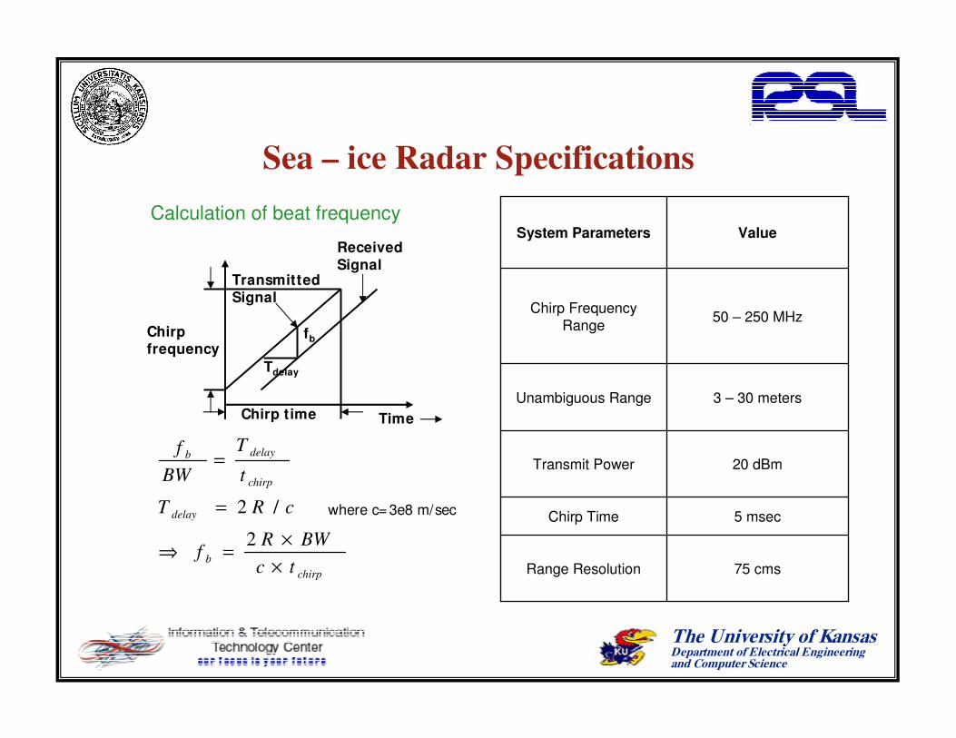
Sea – ice Radar SpecificationsCalculation of beat frequency

Chirp time

Chirp frequency

Transmitted Signal

Received Signal

Time

Tdelay

fb

chirpb

delay

chirp

delayb

tcBWR

f

cRT

t

T

BWf

××=⇒

=

=

2

/2 where c= 3e8 m/sec

75 cmsRange Resolution

5 msecChirp Time

20 dBmTransmit Power

3 – 30 metersUnambiguous Range

50 – 250 MHzChirp Frequency Range

ValueSystem Parameters


Need for Time – frequency analysis of Radar range profiles

Fourier Spectrum Variation of signal amplitude in

decibels over distance traveled by radar signal

Amplitude-scope of sea-ice radar range profile from ‘traverse2.bin’

Features Signals of varying amplitudes over

different distances Highest signal peak at 0dB

indicating ‘Top’ of range profile

Drawbacks Prediction of ice-bottom Distinguish surface returns from

noise signals and multiples


Need for Time – frequency analysis (contd…)

Time – frequency spectrum 2 – dimensional analysis

¾ Determine range to a target – function of time¾ Measure the target speed – function of frequency

Indicates position of different layers ¾ Layers are identified by peaks at specific frequencies for all time ¾ Attempts to distinguish between top and bottom of range profiles from other noise signals

Time – varying filtering¾ Separating noise from data signal

The

Uni

vers

ity o

f Kan

sas

Dep

artm

ent o

f Ele

ctric

al E

ngin

eerin

g an

d Co

mpu

ter S

cien

ce

Tim

e –

Freq

uenc

y R

epre

sent

atio

n


Short Time – Fourier Transform (STFT)

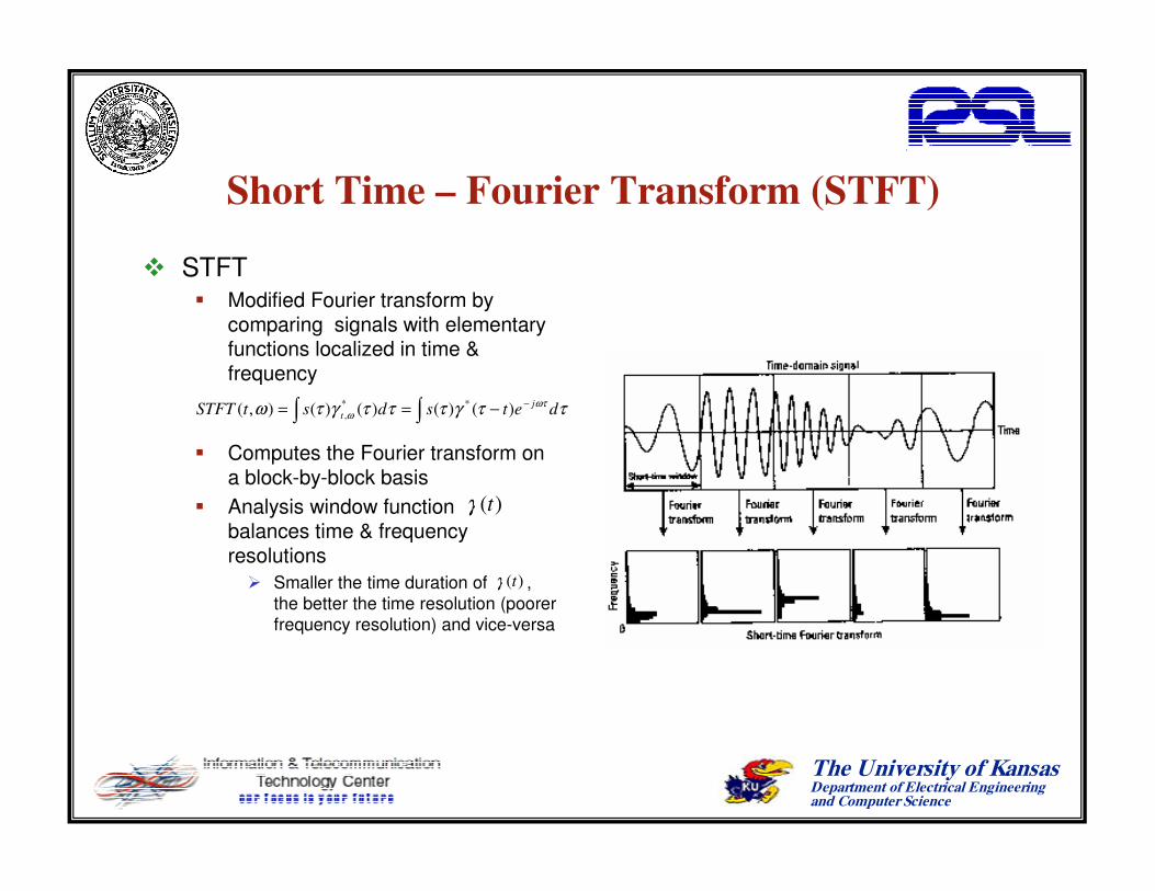
STFT Modified Fourier transform by

comparing signals with elementary functions localized in time & frequency

Computes the Fourier transform on a block-by-block basis

Analysis window function balances time & frequency resolutions

¾ Smaller the time duration of , the better the time resolution (poorer frequency resolution) and vice-versa

∫ ∫ −−== ττγτττγτω ωτω detsdstSTFT j

t )()()()(),( **,

)(tγ

)(tγ


Short – time Fourier transform (contd…)

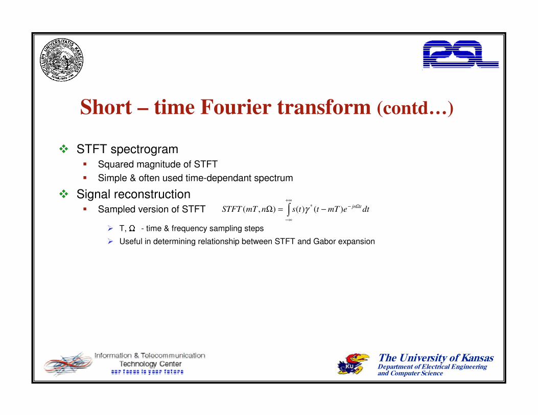
STFT spectrogram Squared magnitude of STFT Simple & often used time-dependant spectrum

Signal reconstruction Sampled version of STFT

¾ T, - time & frequency sampling steps

¾ Useful in determining relationship between STFT and Gabor expansion

∫+∞

∞−

Ω−−=Ω dtemTttsnmTSTFT tjn)()(),( *γ


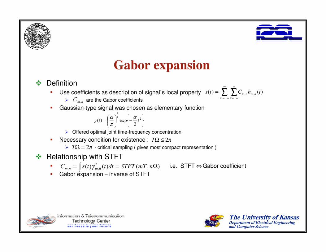
Gabor expansion Definition

Use coefficients as description of signal’s local property ¾ are the Gabor coefficients

Gaussian-type signal was chosen as elementary function

¾ Offered optimal joint time-frequency concentration

Necessary condition for existence : ¾ - critical sampling ( gives most compact representation )

Relationship with STFT i.e. STFT Gabor coefficient Gabor expansion – inverse of STFT

∑ ∑∞

−∞=

∞

−∞=

=m n

nmnm thCts )()( ,,

nmC ,

−

= 24

1

2exp)( ttg

απα

π2=ΩT

⇔

π2≤ΩT

∫ Ω== ),()()( *,, nmTSTFTdtttsC nmnm γ


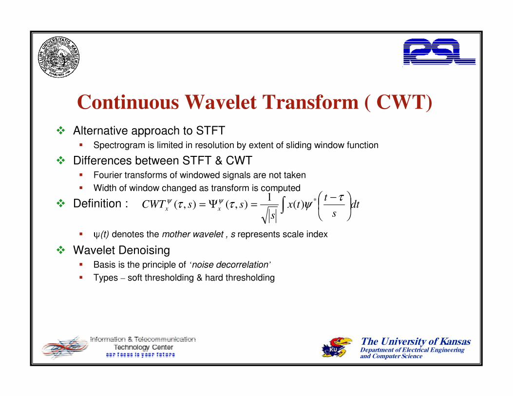
Continuous Wavelet Transform ( CWT) Alternative approach to STFT

Spectrogram is limited in resolution by extent of sliding window function

Differences between STFT & CWT Fourier transforms of windowed signals are not taken Width of window changed as transform is computed

Definition :

(t) denotes the mother wavelet , s represents scale index

Wavelet Denoising Basis is the principle of ‘noise decorrelation’ Types – soft thresholding & hard thresholding

∫

−=Ψ= dt

st

txs

ssCWT xx

τψττ ψψ *)(1

),(),(


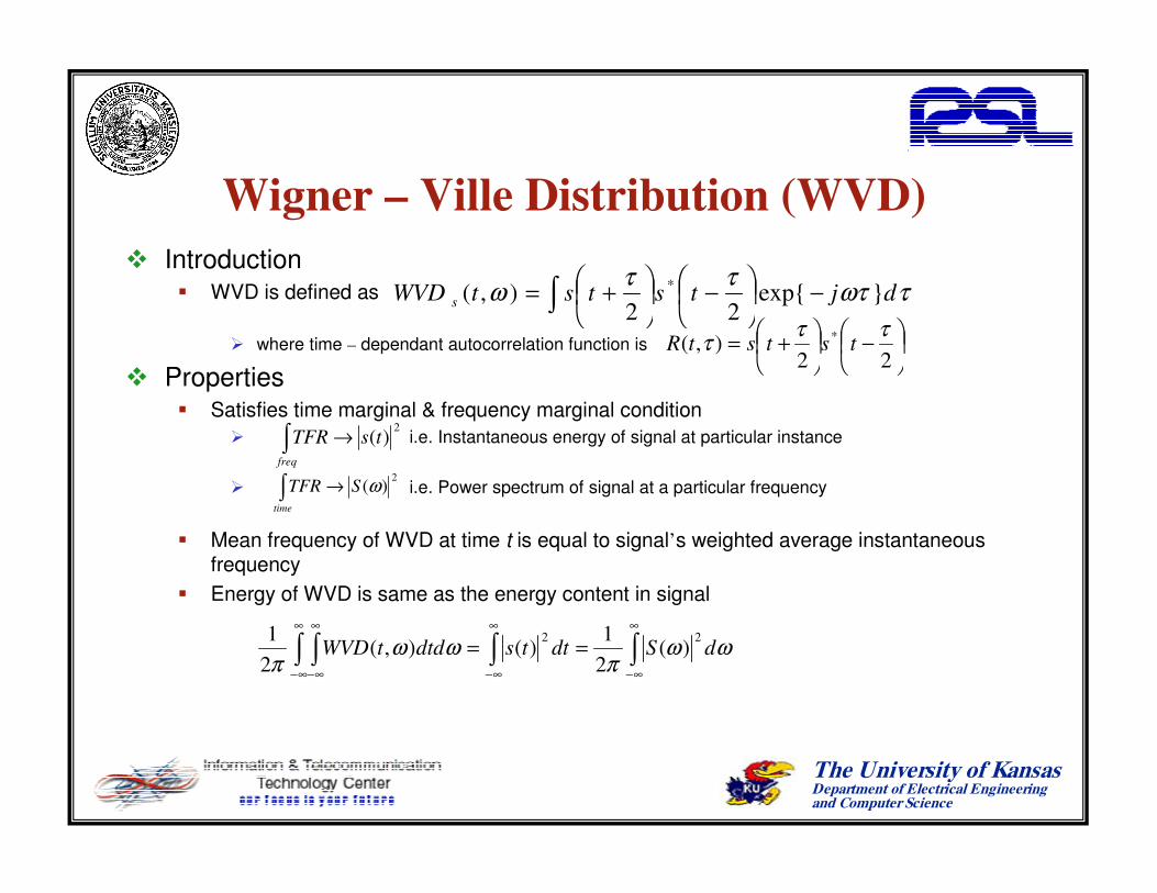
Wigner – Ville Distribution (WVD) Introduction

WVD is defined as

¾ where time – dependant autocorrelation function is

Properties Satisfies time marginal & frequency marginal condition

¾ i.e. Instantaneous energy of signal at particular instance

¾ i.e. Power spectrum of signal at a particular frequency

Mean frequency of WVD at time t is equal to signal’s weighted average instantaneous frequency

Energy of WVD is same as the energy content in signal

−

+=

22),( * τττ tststR

∫ −

−

+= τωτττω djtststWVD s exp

22),( *

2)(tsTFR

freq

→∫2

)(ωSTFRtime

→∫

∫ ∫ ∫ ∫∞

∞−

∞

∞−

∞

∞−

∞

∞−

== ωωπ

ωωπ

dSdttsdtdtWVD22

)(21

)(),(21


Wigner – Ville Distribution ( contd…) Advantages

No window effect Better time & frequency resolutions compared to STFT spectrogram

Drawbacks Cross – term interference

¾ 2 points of TFR interfere to create a contribution on 3rd point located at their geometrical midpoint¾ Oscillate perpendicularly to line joining two points interfering, with a frequency proportional to

distance between two points

Alternatives Cohen’s class of distributions Gabor spectrogram


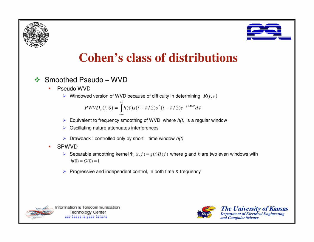
Cohen’s class of distributions Smoothed Pseudo – WVD

Pseudo WVD¾ Windowed version of WVD because of difficulty in determining

¾ Equivalent to frequency smoothing of WVD where h(t) is a regular window

¾ Oscillating nature attenuates interferences

¾ Drawback : controlled only by short – time window h(t)

SPWVD¾ Separable smoothing kernel where g and h are two even windows with

¾ Progressive and independent control, in both time & frequency

),( τtR

∫∞

∞−

−−+= ττττυ πυτ detstshtPWVD js

2* )2/()2/()(),(

)()(),( fHtgftT =Ψ1)0()0( == Gh


Choi – Williams Distribution Kernel design

Theory of interference distributions - developed by Choi & Williams

Exponential kernel: where is scaling parameter

Properties Suppresses the cross-terms created by two functions having different time & frequency

centers controls the decay speed

¾ as decreases the interference is reduced

¾ When we obtain the WVD.

Essentially a low – pass filter in plane which preserves properties of WVD while reducing cross-term interference

2

)(exp),(

2

2

σπϑττϑ −=Φ

∞→σ

),τν(


Time – Variant Filter Application of TFR

Detection & estimation of noise-corrupted signals SNR is substantially improved in joint time-frequency domain

Filtering mechanism Based on both linear & bilinear time-frequency representations Gabor expansion-based filter is most widely used

Techniques Least Square Error (LSE) filter Iterative Time – Variant Filter


Experiments & Results – Outline Ideal Simulations

Sum of frequency tones Linear chirp signal

Sea – ice radar data Measured depth from field tests How does TFD distinguish surface return from noise ?

Time – frequency techniques Linear transforms – STFT Quadratic transforms – WVD, SPWVD, CWD

Time – variant filtering Drawbacks of aforementioned techniques Wavelet denoising


Ideal Simulations Test of TFR with cosine signal

Input frequency tones :

where and

Power spectrum does not indicate when frequency tones occur

TFR results Frequency tones at 50KHz & 150KHz

varying from (0-2ms), (2.5-4.5ms) Image frequencies at 200KHz and

100KHz respectively Differences in amplitudes indicated by

respective colormap scales of frequency tones

KHzfbTsnfbnx

KHzfaTsnfanx

150;1),***2cos(][

50;5.0),***2cos(][

2222

1111

======

ππ

2249:1250,999:0 21 == nn

KhzTsf s 500/1 ==

][][][ 21 nxnxnx +=


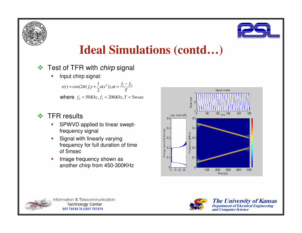
Ideal Simulations (contd…) Test of TFR with chirp signal

Input chirp signal:

where

TFR results SPWVD applied to linear swept-

frequency signal Signal with linearly varying

frequency for full duration of time of 5msec

Image frequency shown as another chirp from 450-300KHz

Tff

ttfts 0120 )),.

21

(2cos()(−=+= ααπ

sec5,200,50 10 mTKhzfKhzf ===


Sea – ice radar experimental data

Sea-ice (FMCW) radar Data set from field experiments in

Barrow, Alaska Measured sea-ice depth compared

with depth calculated from signal processing experiments

Ice thickness data Field experiments show the measured

ice thickness at various depths Ascope-60 of file traverse2.bin at

distance of 0-20m from 1st point Calculations suggest

¾ Antenna feedthrough – 3.45m¾ Ice bottom – 7.35m


How does TFD distinguish surface return from noise ?

Frequency is expressed as function of distance or range

Time – dependant spectrum expresses variation of beat signal at different instances of time for a given frequency

Presence of surface return Signal exists for entire duration of time interval at given frequency Otherwise, signal is assumed to be noise or multiple return


STFT – based Spectrogram

Narrow Window Good time resolution & poor

frequency resolution Peaks are well separated from each

other in time In frequency domain, every peak

covers a range of frequencies instead of a single frequency

Wide Window Good frequency resolution & poor time

resolution Frequency resolution is much better

with continuous variation in time In time domain, peaks are not

observed


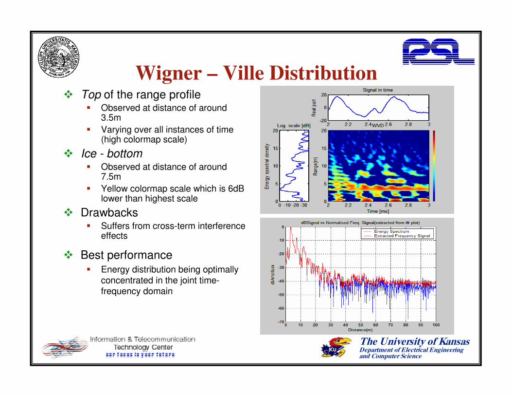
Wigner – Ville Distribution Top of the range profile

Observed at distance of around 3.5m

Varying over all instances of time (high colormap scale)

Ice - bottom Observed at distance of around

7.5m Yellow colormap scale which is 6dB

lower than highest scale

Drawbacks Suffers from cross-term interference

effects

Best performance Energy distribution being optimally

concentrated in the joint time-frequency domain


Smoothed Pseudo WVD

Defined by smoothing kernel

g & h are time and frequency smoothing windows respectively

Trade – off Improves the cross-term

interference at the cost of lower resolution

More the smoothing in time and/or frequency, the poorer the resolution in time and/or frequency

Surface returns clearly visible

)()(),( fHtgftT =ψ


Choi – Williams Distribution

Employs the exponential kernel

where is a scaling factor Effect of :

¾ cross-terms diminish in size¾ width of the signal component

spreads ¾ surface returns distinguished easily ¾ mild loss in resolution

¾ approaches the Wigner transform,

since the kernel is nearly constant¾ interference terms become more

prominent¾ Frequency & time resolution are

comparable to that of WVD

/exp),( 22 σττψ vv −=σ

σ01.0=σ

∞→σ


Time – Variant Filtering

Time – variant denoising Investigated for FMCW radar signals Discrete Gabor transform is used Not suitable for radar chirp signals

Wavelet denoising Radar echogram showing the noisy

signal

Alternative Wavelet transforms can be used Currently used for ‘depth sounder

radar’ in RSL

SNR of denoised signal : 1.4 dB (clean signal)


CONCLUSIONS Comparison between Fourier analysis & Joint time – frequency analysis

Time – frequency analysis Classification Need for TFA of radar range profiles

Time – variant filtering Discrete Gabor transform cannot be used

Signal processing experiments STFT spectrogram – worst resolutions WVD – best performance / optimal concentration in joint time-frequency domain

¾ surface returns clearly visible¾ Depth from radar matched that of measured depth

Cohen’s class of distributions – compromise between interference reduction & loss in resolution


FUTURE WORK

Wavelet denoising can be investigated for FMCW radars

Time – variant filtering can be attempted for other radar signals Particularly for moving targets

Applications of Time – frequency analysis Speech & music signal processing

The

Uni

vers

ity o

f Kan

sas

Dep

artm

ent o

f Ele

ctric

al E

ngin

eerin

g an

d Co

mpu

ter S

cien

ce

time frequency analysis – an application to fmcw … · time frequency analysis – an...

Documents