estimation and compensation of frequency sweep nonlinearity … · · 2017-06-01estimation and...
TRANSCRIPT

1
Estimation and compensation of frequency sweep nonlinearity in FMCW
radar
by
Kurt Peek
Picture: www.thalesgroup.com
A thesis submitted in partial fulfillment
Of the requirements for the degree of
MASTER OF SCIENCE in APPLIED MATHEMATICS
Supervisors: Gjerrit Meinsma, Anton Stoorvogel

2
Table of Contents Abstract ................................................................................................................................................... 4
1 Introduction .................................................................................................................................... 5
1.1 ‘Hardware’ sweep linearization .............................................................................................. 9
1.2 ‘Software’ linearization techniques ...................................................................................... 10
1.3 This thesis .............................................................................................................................. 11
2 Theory of operation of FMCW radar ............................................................................................ 12
2.1 Analytical model of a FMCW radar ....................................................................................... 12
2.1.1 Transmitted signal ......................................................................................................... 12
2.1.2 Received signal .............................................................................................................. 13
2.1.3 Dechirped signal ............................................................................................................ 14
2.1.4 Video signal ................................................................................................................... 18
2.2 The effect of sinusoidal nonlinearity in the frequency sweep .............................................. 20
2.2.1 Analytical development ................................................................................................ 20
3 An algorithm for compensating the effect of phase errors on the FMCW beat signal spectrum 25
3.1 Prior work .............................................................................................................................. 25
3.2 Mathematical preliminaries .................................................................................................. 26
3.2.1 The quadratic phase filter ............................................................................................. 26
3.2.2 The Fresnel transform ................................................................................................... 26
3.3 Description of the phase error compensation algorithm ..................................................... 27
3.4 Derivation of the algorithm for temporally infinite chirps ................................................... 30
3.4.1 Recapitulation of the FMCW principle for linear chirps ............................................... 30
3.4.2 Introduction of phase errors ......................................................................................... 31
3.4.3 First step: removal of phase errors emanating from the transmitted signal ............... 32
3.4.4 Second step: range deskew .......................................................................................... 32
3.4.5 Third step: removal of residual phase errors ................................................................ 34
3.4.6 Comparison with Meta’s algorithm .............................................................................. 35
3.4.7 Narrowband IF signals: comparison with Burgos-Garcia’s algorithm ........................... 35
3.5 Application of the algorithm to finite chirps ......................................................................... 36
3.5.1 Compensation algorithm for narrowband IF signals .................................................... 36
3.5.2 Application to sinusoidal phase errors.......................................................................... 39
4 Simulation ..................................................................................................................................... 45
4.1 Digital implementation of the phase error compensation method ..................................... 45
4.2 Implementation of the deskew filter by the frequency sampling method .......................... 45

3
4.2.1 The frequency sampling method and time-domain aliasing ........................................ 46
4.2.2 Number of FFT points required to prevent time-domain aliasing ................................ 47
4.2.3 Approximating the input signal spectrum .................................................................... 48
4.2.4 Multiplication by the exact deskew filter frequency response..................................... 49
4.2.5 Inverse Fourier transform of the spectrum of the output ............................................ 50
4.2.6 Implementation of the deskew filter as a MATLAB function ....................................... 50
4.2.7 Test of the deskew filter for a known, exact output ..................................................... 51
4.3 Simulation of the phase error compensation algorithm ...................................................... 53
4.4 Results for cases of interest .................................................................................................. 56
4.4.1 Sinusoidal phase errors ................................................................................................. 56
4.4.2 Power-law phase errors ................................................................................................ 58
4.5 Concluding remarks .............................................................................................................. 60
5 Estimation of the phase errors ..................................................................................................... 62
5.1 Review of a known method using a reference delay ............................................................ 62
5.2 Proposal of a novel method using ambiguity functions ....................................................... 62
6 Conclusions and discussion ........................................................................................................... 64
Bibliography .......................................................................................................................................... 65
MATLAB simulation ............................................................................................................................... 69
4
Abstract One of the main issues limiting the range resolution of linear frequency-modulated continuous-wave
(FMCW) radars is nonlinearity of frequency sweep, which results in degradation of contrast and
range resolution, especially at long ranges. Two novel, slightly different, methods to correct for
nonlinearities in the frequency sweep by digital post-processing of the deramped signal were
introduced independently by Burgos-Garcia et al. (Burgos-Garcia, Castillo et al. 2003) and Meta et al.
(Meta, Hoogeboom et al. 2006). In these publications, however, no formal proof of the techniques
was given, and no limitations were described. In this thesis, we prove that the algorithm of Meta is
exact for temporally infinite chirps, and remains valid for finite chirps with large time-bandwidth
products provided the maximum frequency component of the phase error function is sufficiently
low. It is also shown that the algorithm of Meta reduces to that of Burgos-Garcia in this limit. A
digital implementation of the method is described. We also propose a novel method to measure the
systematic phase errors which are required as input to the compensation algorithm. The applicability
of this technique to the field of optical frequency domain reflectometry (OFDR) is noted.

5
1 Introduction Frequency-modulated continuous-wave (FMCW) radars provide high range measurement precision
and high range resolution at moderate hardware expense (Griffiths 1990; Stove 1992). Moreover,
the spreading of the transmitted power over a large bandwidth provides makes FMCW radar difficult
to detect by intercept receivers, providing it with stealth in military applications. In the last two
decades, Thales Netherlands has developed a family of silent radars for air surveillance, coastal
surveillance, navigation, and ground surveillance based on FMCW technology.
In FMCW radar, the range to the target is measured by systematically varying the frequency of a
transmitted radio frequency (RF) signal. Typically, the transmitted frequency is made to vary linearly
with time; for example, a sawtooth or triangular frequency sweep is implemented. The linear
variation of frequency with time is referred to as a chirp, frequency sweep, or frequency ramp. Figure
1 shows a time-frequency plot of a linear sawtooth FMCW transmit signal and its corresponding
amplitude.
6
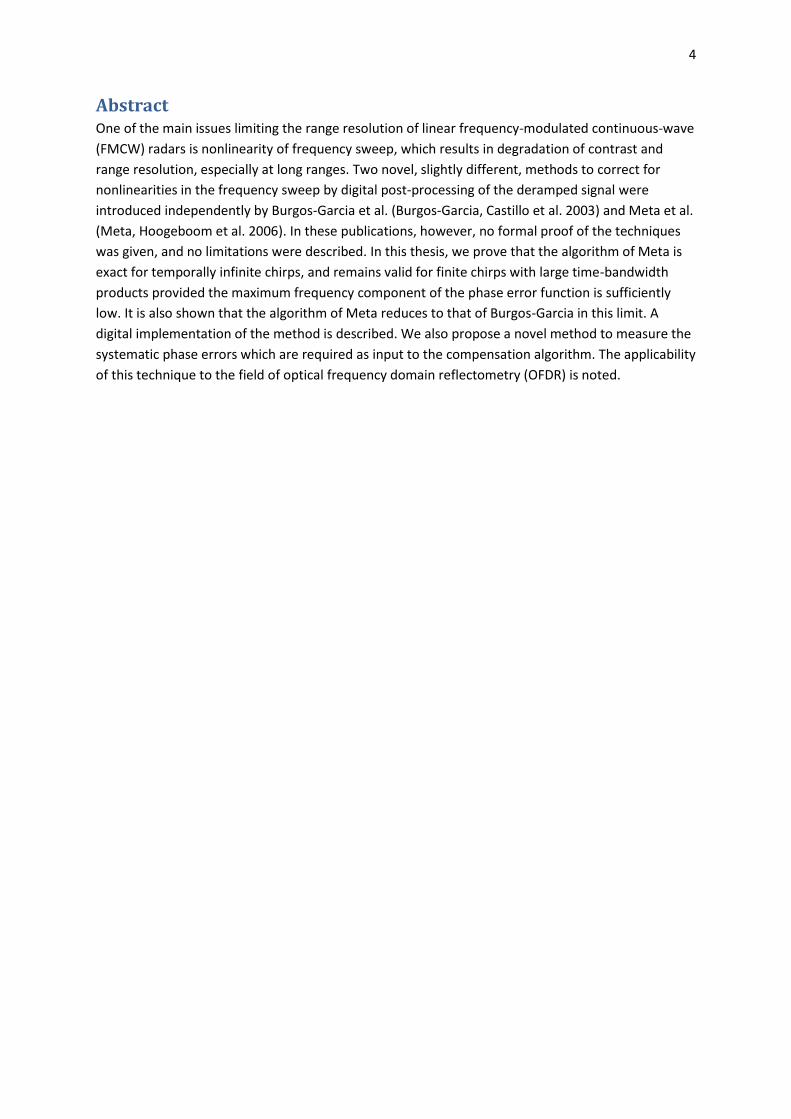
Figure 1 (a) Time-frequency plot of a FMCW transmit signal with carrier frequency , sweep period , and bandwidth1
. Typical parameters are = 10 GHz, = 500 μs, and = 50 MHz. (b) Time-amplitude plot of a transmitted FMCW signal (not with the parameters listed above).
The frequency sweep effectively places a “time stamp” on the transmitted signal at every instant,
and the frequency difference between the transmitted signal and the signal returned from the target
(i.e. the reflected or received signal) can be used to provide a measurement of the target range, as
illustrated in Figure 2. This process is called dechirping or deramping, and the frequency of the
dechirped signal is called the beat or intermediate frequency (IF) signal.
1 The term ‘bandwidth’ is often used in this context to refer to the total excursion of the instantaneous
frequency during one the sweep period. The FMCW signal is not bandlimited in the mathematical sense of the word; however, for large time-bandwidth products it is approximately bandlimited.
time
time
instantaneous
frequency
amplitude
bandwidth
𝐵 = 50 MHz
sweep period
𝑇 = 500 µs
carrier
frequency
𝑓𝑐 = 10 GHz
(a)
(b)
7
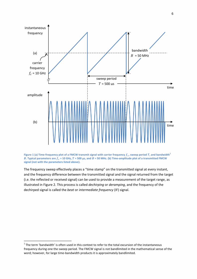
Figure 2 Principle of FMCW range measurement. (a) Time-frequency plots of the transmitted chirp (solid line) and the echoes from two ‘point’ targets (dashed lines), delayed by their respective two-way propagation delays to the target and back. (b) Time-frequency plots of the frequency difference, or ‘beat frequency’, between the transmitted and received chirps. The beat frequency is observed during portion of the sweep period in which the transmitted and received signals overlap.
As seen from Figure 2, the target transit time and target beat frequency are directly proportional,
and their proportionality constant is equal to the chirp rate (i.e., the ratio between the bandwidth
and the sweep period) of the transmitted chirp. Hence, the target transit time – and thus, the target
range – can be inferred by a measurement of the beat frequency.
The beat frequency is generated in the receiver of the FMCW radar by a mixer2 or ‘multiplier’ as
illustrated in Error! Reference source not found.. The local oscillator (LO) port of the mixer is fed by
a portion of the transmit signal3, while the radio frequency (RF) port is fed by the target echo signal
from the receive antenna. As explained in more detail in Section 2.1.3, the output of the mixer,
called the intermediate frequency (IF) signal, has a phase which (after low-pass filtering) is the
2 A mixer is a three-port device that uses a nonlinear or time-varying element to achieve frequency conversion
(Pozar 2005). In its down-conversion configuration, it has two inputs, the radio frequency (RF) signal and the local oscillator (LO) signal. The output, or intermediate frequency (IF) signal, of an idealized mixer is given by the product of RF and LO signals. 3 This is the homodyne receiver architecture, in which the local oscillator signal is provided by the transmitter
itself. Alternatively, the local oscillator can be generated separately and triggered at an appropriate instant; this is commonly referred to as stretch processing (Caputi 1971). Stretch processing has the disadvantage of the additional complexity of another oscillator. Receiver noise effects will also be greater because of the independence of the phase noise of the separate oscillators (Piper 1993).
transmitted
linear chirp
received
target echoes
frequency
after
dechirping
instantaneous
transmit
frequency
time
time
target beat
signals
target round-
trip delays
target beat
frequencies
8
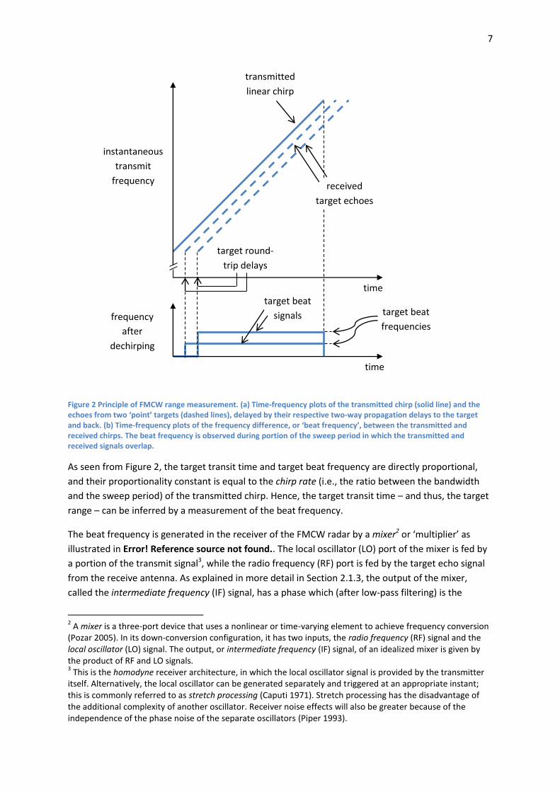
difference of the phases of the LO and RF signals. Hence, its frequency is the ‘beat ‘frequency
described above. The beat signal is passed to a spectrum analyzer, which is a bank of filters used to
resolve targets in to range bins. Typically, the spectrum analyzer is implemented as an analog-to-
digital converter (ADC) followed by a processor based on the fast Fourier transform (FFT).
Figure 3 Simplified block diagram of a homodyne FMCW radar transceiver. A chirp generator generates a linear sawtooth FMCW signal (left, upper inset) which is radiated out to the target scene by a transmit antenna. A portion of the transmitted signal is coupled to the local oscillator (LO) port of a mixer. The target echo received by a separate receive antenna is fed to the radio frequency (RF) port of the mixer. The mixer output at intermediate frequency (IF) is fed to a spectrum analyzer. The output of the spectrum analyzer for a single target is a ‘sinc’ function centered at the target beat frequency (left, lower inset).
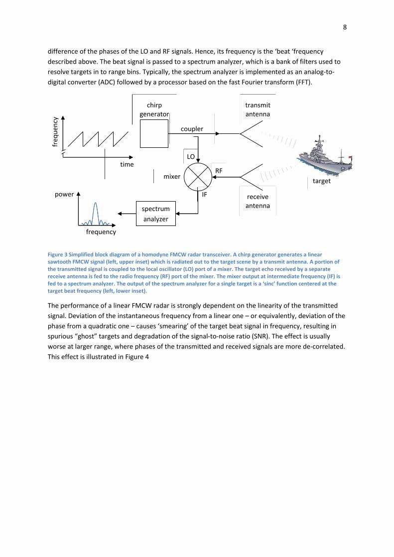
The performance of a linear FMCW radar is strongly dependent on the linearity of the transmitted
signal. Deviation of the instantaneous frequency from a linear one – or equivalently, deviation of the
phase from a quadratic one – causes ‘smearing’ of the target beat signal in frequency, resulting in
spurious “ghost” targets and degradation of the signal-to-noise ratio (SNR). The effect is usually
worse at larger range, where phases of the transmitted and received signals are more de-correlated.
This effect is illustrated in Figure 4
chirp generator
spectrum
analyzer
time
coupler
mixer
transmit antenna
freq
uen
cy
receive antenna
target
RF
LO
IF
frequency
power
9
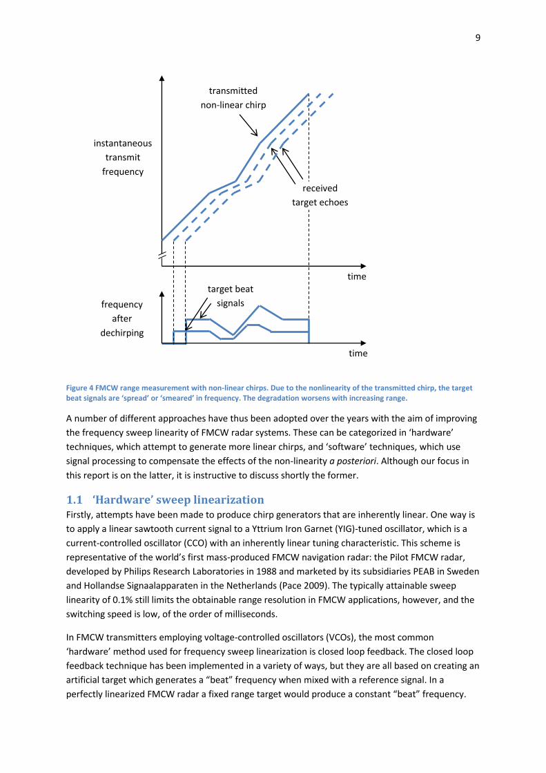
Figure 4 FMCW range measurement with non-linear chirps. Due to the nonlinearity of the transmitted chirp, the target beat signals are ‘spread’ or ‘smeared’ in frequency. The degradation worsens with increasing range.
A number of different approaches have thus been adopted over the years with the aim of improving
the frequency sweep linearity of FMCW radar systems. These can be categorized in ‘hardware’
techniques, which attempt to generate more linear chirps, and ‘software’ techniques, which use
signal processing to compensate the effects of the non-linearity a posteriori. Although our focus in
this report is on the latter, it is instructive to discuss shortly the former.
1.1 ‘Hardware’ sweep linearization Firstly, attempts have been made to produce chirp generators that are inherently linear. One way is
to apply a linear sawtooth current signal to a Yttrium Iron Garnet (YIG)-tuned oscillator, which is a
current-controlled oscillator (CCO) with an inherently linear tuning characteristic. This scheme is
representative of the world’s first mass-produced FMCW navigation radar: the Pilot FMCW radar,
developed by Philips Research Laboratories in 1988 and marketed by its subsidiaries PEAB in Sweden
and Hollandse Signaalapparaten in the Netherlands (Pace 2009). The typically attainable sweep
linearity of 0.1% still limits the obtainable range resolution in FMCW applications, however, and the
switching speed is low, of the order of milliseconds.
In FMCW transmitters employing voltage-controlled oscillators (VCOs), the most common
‘hardware’ method used for frequency sweep linearization is closed loop feedback. The closed loop
feedback technique has been implemented in a variety of ways, but they are all based on creating an
artificial target which generates a “beat” frequency when mixed with a reference signal. In a
perfectly linearized FMCW radar a fixed range target would produce a constant “beat” frequency.
transmitted
non-linear chirp
received
target echoes
frequency
after
dechirping
instantaneous
transmit
frequency
time
time
target beat
signals
10
Therefore, in a practical FMCW radar, if the “beat” frequency drifts from the desired constant
frequency value, an error signal can be generated to fine-tune the VCO to maintain a constant
“beat” frequency. This feedback technique can be implemented at the final RF frequency of the
radar or at a lower, down-converted frequency. Waveforms having sweep linearity4 better than
0.05% have been demonstrated {Fuchs, 1996 #181} but, unless the system is very well designed, the
technique can be prone to instabilities and is typically limited in bandwidth to about 600 MHz. Also,
because the VCO is modulated directly, the phase noise of the resultant transmit signal can be
compromised (Beasley 2009).
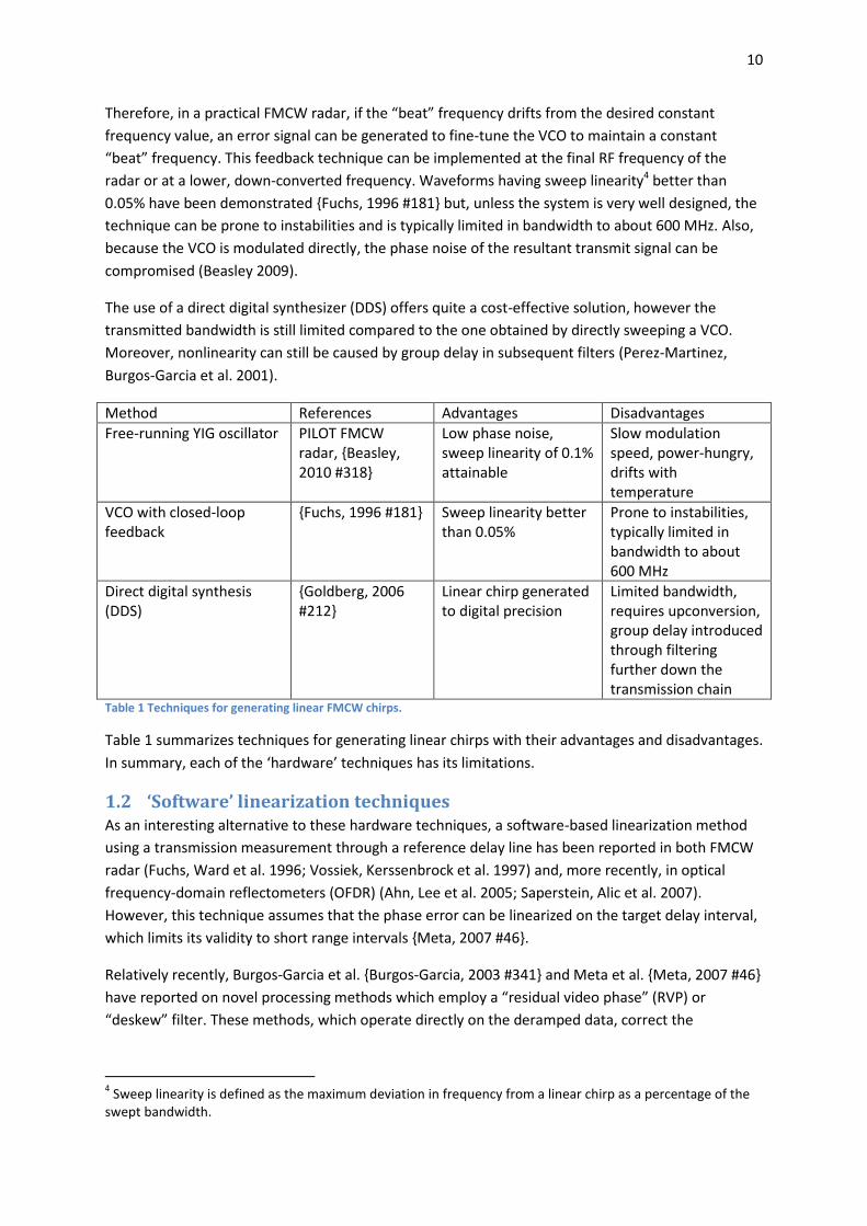
The use of a direct digital synthesizer (DDS) offers quite a cost-effective solution, however the
transmitted bandwidth is still limited compared to the one obtained by directly sweeping a VCO.
Moreover, nonlinearity can still be caused by group delay in subsequent filters (Perez-Martinez,
Burgos-Garcia et al. 2001).
Method References Advantages Disadvantages
Free-running YIG oscillator PILOT FMCW radar, {Beasley, 2010 #318}
Low phase noise, sweep linearity of 0.1% attainable
Slow modulation speed, power-hungry, drifts with temperature
VCO with closed-loop feedback
{Fuchs, 1996 #181} Sweep linearity better than 0.05%
Prone to instabilities, typically limited in bandwidth to about 600 MHz
Direct digital synthesis (DDS)
{Goldberg, 2006 #212}
Linear chirp generated to digital precision
Limited bandwidth, requires upconversion, group delay introduced through filtering further down the transmission chain
Table 1 Techniques for generating linear FMCW chirps.
Table 1 summarizes techniques for generating linear chirps with their advantages and disadvantages.
In summary, each of the ‘hardware’ techniques has its limitations.
1.2 ‘Software’ linearization techniques As an interesting alternative to these hardware techniques, a software-based linearization method
using a transmission measurement through a reference delay line has been reported in both FMCW
radar (Fuchs, Ward et al. 1996; Vossiek, Kerssenbrock et al. 1997) and, more recently, in optical
frequency-domain reflectometers (OFDR) (Ahn, Lee et al. 2005; Saperstein, Alic et al. 2007).
However, this technique assumes that the phase error can be linearized on the target delay interval,
which limits its validity to short range intervals {Meta, 2007 #46}.
Relatively recently, Burgos-Garcia et al. {Burgos-Garcia, 2003 #341} and Meta et al. {Meta, 2007 #46}
have reported on novel processing methods which employ a “residual video phase” (RVP) or
“deskew” filter. These methods, which operate directly on the deramped data, correct the
4 Sweep linearity is defined as the maximum deviation in frequency from a linear chirp as a percentage of the
swept bandwidth.

11
nonlinearity effects for the whole range profile at once, and are based only on the assumption that
the transmitted chirp has a large time-bandwidth product.
1.3 This thesis The algorithms proposed by Burgos-Garcia et al. {Burgos-Garcia, 2003 #341} and Meta et al. {Meta,
2007 #46} are actually slightly different. Further, they are presented based on heuristic reasoning;
no formal proof is given, and no limitations of the algorithm are mentioned.
This thesis makes three main contributions to knowledge:
(1) We give a proof of both Meta’s “wideband” and Burgos-Garcia’s “narrowband” variations of
the phase error compensation algorithm. It is shown that the algorithm of Meta reduces to
that of Burgos-Garcia in the special case that the error frequency components are
sufficiently low. Further, our analytical results indicate that the original algorithm as
presented by Meta {Meta, 2006 #340}{Meta, 2007 #46} contains a sign error. Finally, we
discuss issues which arise when applying the algorithm to time-limited chirps, which have
not been discussed previously.
(2) We implement both phase error compensation algorithms in MATLAB and demonstrate
their effectiveness. (In {Burgos-Garcia, 2003 #341} and {Meta, 2007 #46}, no detail was given
on the digital implementation of the algorithm). The results of our simulation are
inconclusive, however, as to whether there is a minus sign error in Meta’s derivation or not.
Further improvements to the simulation algorithm, which involve taking into account the
“edge effects” due to the time-limited nature of the chirps, are proposed.
(3) We propose a novel method for determining the phase errors using measurements from
targets at different reference delays, based on the synthesis problem of a function from its
ambiguity function as discussed by Wilcox {Wilcox, 1991 #391}. The novel method could
have advantages over known methods, which use just a single reference delay.
The organization of this thesis is as follows. In Chapter 2, we discuss the theory of operation of
FMCW radar in more mathematical detail. In Chapter 3, we derive both variations of the phase error
compensation algorithm analytically and address the issues mentioned above in point (1). In Chapter
0, we perform a simulation of the algorithms and demonstrate their effectiveness. In Chapter 5, we
discuss the estimation of phase errors, which are required as input for the algorithm. Finally, in
Chapter 6, we wrap up with our conclusions and discussion.
12
2 Theory of operation of FMCW radar This chapter presents a tutorial review of the basic principles of FMCW (frequency modulated
continuous wave) radars. The material to follow is on homodyne FMCW radar, i.e., CW radar in
which a microwave oscillator is frequency-modulated and serves as both transmitter and local
oscillator (Skolnik 2008). The effect of frequency sweep nonlinearity is also discussed.
An outline of this chapter is as follows. In Section 2.1, we present an analytical model of the
generation of the target range profile by a FMCW transmitting ideal linear chirps. In Section 2.2, we
discuss how its performance is affected by sinusoidal frequency sweep nonlinearities.
2.1 Analytical model of a FMCW radar In this section, we explain the principle FMCW range measurement in more mathematical detail. In
Section 2.1.1, we formulate an expression for the transmitted signal. In Section 2.1.2, we construct a
model for the received signal. In Section 2.1.3, we explain the generation of the ‘dechirped’,
‘deramped’, or ‘beat’ signal. Of particular importance for the algorithm to be described is the use of
‘coherent detection’ to obtain complex samples of this signal. Finally, in Section 2.1.4, we discuss the
spectrum of the beat signal or ‘video signal’, which is used to visualize the target scene.
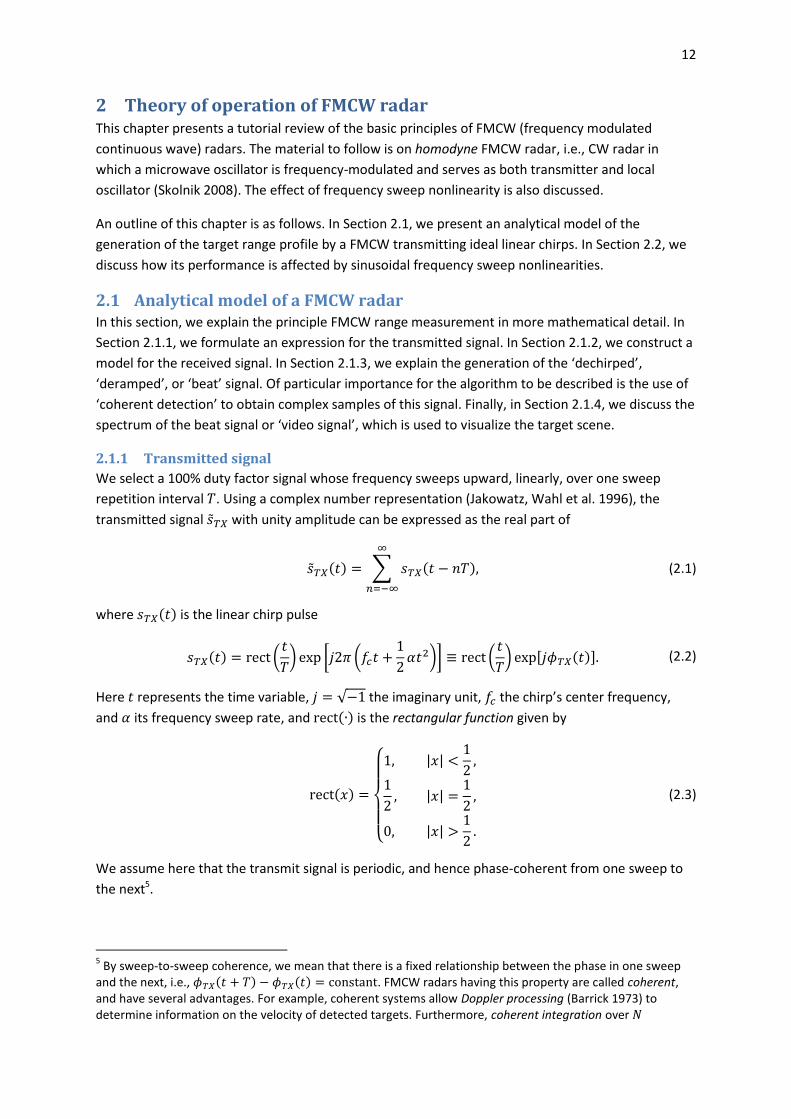
2.1.1 Transmitted signal
We select a 100% duty factor signal whose frequency sweeps upward, linearly, over one sweep
repetition interval . Using a complex number representation (Jakowatz, Wahl et al. 1996), the
transmitted signal with unity amplitude can be expressed as the real part of
( ) ∑ ( )
(2.1)
where ( ) is the linear chirp pulse
( ) (
) [ (
)] (
) , ( )- (2.2)
Here represents the time variable, √ the imaginary unit, the chirp’s center frequency,
and its frequency sweep rate, and ( ) is the rectangular function given by
( )
{
| |
| |
| |
(2.3)
We assume here that the transmit signal is periodic, and hence phase-coherent from one sweep to
the next5.
5 By sweep-to-sweep coherence, we mean that there is a fixed relationship between the phase in one sweep
and the next, i.e., ( ) ( ) . FMCW radars having this property are called coherent, and have several advantages. For example, coherent systems allow Doppler processing (Barrick 1973) to determine information on the velocity of detected targets. Furthermore, coherent integration over

13
Since the instantaneous frequency, ( ), is the derivative of the phase (Carson 1922), we have
( )
(2.4)
Thus it can be seen that the frequency excursion over one sweep repetition interval is , the
chirp bandwidth. The instantaneous frequency of the transmit signal is plotted in Figure 5(a) as the
solid line.
Figure 5 Time-frequency plots of (a) the transmitted (solid line) and received (dashed line) signals, and (b) the intermediate frequency (IF) signal. The IF alternates between two distinct tones: for intervals of duration and ( ) for intervals of duration , where is the frequency sweep rate. Typical chirp parameters for an FMCW navigation radar are = 10 GHz, = 50 MHz, and = 500 μs.
2.1.2 Received signal
After transmission of the radar signal through the transmit antenna, the radar waveform propagates
to the target scene, and part of the energy is scattered back to the radar’s receive antenna. In the
following analytical development, we assume that the target scene consists of a single stationary
‘point’ target such that the echo signal ( ) is simply a delayed replica of the transmit signal:
( ) ( ) (2.5)
where is the two-way propagation delay given by
frequency sweeps improves the signal-to-noise ratio (SNR) by a factor of . This should be contrasted with the
SNR increase of √ typically obtained using incoherent integration of frequency sweeps (Beasley 2009).
𝜏
time
𝑓𝑏1 𝛼𝜏
𝑇
𝐵
𝑓𝑐
𝑇 𝜏
𝑓𝑏 𝛼(𝑇 𝜏)
(a)
(b)
time
target echo
transmitted chirp
beat signal
frequency
frequency
14
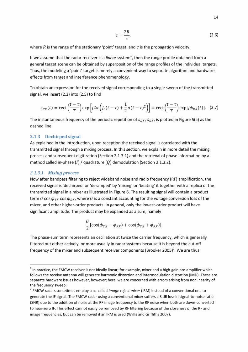
(2.6)
where is the range of the stationary ‘point’ target, and is the propagation velocity.
If we assume that the radar receiver is a linear system6, then the range profile obtained from a
general target scene can be obtained by superposition of the range profiles of the individual targets.
Thus, the modeling a ‘point’ target is merely a convenient way to separate algorithm and hardware
effects from target and interference phenomenology.
To obtain an expression for the received signal corresponding to a single sweep of the transmitted
signal, we insert (2.2) into (2.5) to find
( ) (
) [ ( ( )
( ) )] (
) , ( )- (2.7)
The instantaneous frequency of the periodic repetition of , , is plotted in Figure 5(a) as the
dashed line.
2.1.3 Dechirped signal
As explained in the Introduction, upon reception the received signal is correlated with the
transmitted signal through a mixing process. In this section, we explain in more detail the mixing
process and subsequent digitization (Section 2.1.3.1) and the retrieval of phase information by a
method called in-phase ( ) / quadrature ( ) demodulation (Section 2.1.3.2).
2.1.3.1 Mixing process
Now after bandpass filtering to reject wideband noise and radio frequency (RF) amplification, the
received signal is ‘dechirped’ or ‘deramped’ by ‘mixing’ or ‘beating’ it together with a replica of the
transmitted signal in a mixer as illustrated in Figure 6. The resulting signal will contain a product
term , where is a constant accounting for the voltage conversion loss of the
mixer, and other higher-order products. In general, only the lowest-order product will have
significant amplitude. The product may be expanded as a sum, namely
, ( ) ( )-
The phase-sum term represents an oscillation at twice the carrier frequency, which is generally
filtered out either actively, or more usually in radar systems because it is beyond the cut-off
frequency of the mixer and subsequent receiver components (Brooker 2005)7. We are thus
6 In practice, the FMCW receiver is not ideally linear; for example, mixer and a high-gain pre-amplifier which
follows the receive antenna will generate harmonic distortion and intermodulation distortion (IMD). These are separate hardware issues however, however; here, we are concerned with errors arising from nonlinearity of the frequency sweep. 7 FMCW radars sometimes employ a so-called image reject mixer (IRM) instead of a conventional one to
generate the IF signal. The FMCW radar using a conventional mixer suffers a 3 dB loss in signal-to-noise ratio
(SNR) due to the addition of noise at the RF image frequency to the RF noise when both are down-converted
to near-zero IF. This effect cannot easily be removed by RF filtering because of the closeness of the RF and
image frequencies, but can be removed if an IRM is used (Willis and Griffiths 2007).

15
interested in the function
( ), which is called the ‘dechirped’, ‘deramped’, ‘beat’, or
‘intermediate frequency’ (IF) signal. The IF signal with unity amplitude (we do not consider
amplitude variations in this derivation) is thus
( ) ( ) (2.8)
Figure 6 Simplified block diagram of a homodyne FMCW transceiver. The received (RX) signal is fed to the radio frequency (RF) port of a mixer, while a portion of the transmit (TX) signal is coupled to the local oscillator (LO) port. The mixer output is low-pass filtered to obtain the desired intermediate frequency (IF) signal, which is digitized by an analog-to-digital (A/D) converter at a rate of at least twice the maximum beat frequency .
A complex representation of the IF signal resulting from a single pulse of the transmitted signal is
obtained by Inserting (2.2) and (2.7) into (2.8), a single pulse of the IF signal can be expressed as the
real part of
( ) ( ) ( )
(
) (
) [ (
( )
( ) )]
or, simplifying,
( ) ( ) [ (
)] (2.9)
where the beat signal envelope ( ) is given by
( ) {
(2.10)
During the remaining part of the sweep period, on the interval , ⁄ ⁄ -, the received
signal corresponds to the transmitted signal during the previous sweep. Therefore, the mixer output
will be offset by the sweep width, , as illustrated in Figure 5(b). is much greater than the signal
frequency and the mixer output for ⁄ ⁄ will therefore be filtered and rejected.
Hence, for ⁄ ⁄ , the IF signal will be a transient pulse. If a digital data system is
used to observe the mixer output, the sampling can be delayed at the start of each sweep so the
retrace effects of the local oscillator returning to ⁄ are simply omitted (Strauch 1976).
Let us consider the three terms that comprise the phase of the IF signal (2.9):
A/D
mixer low-pass
filter RF
LO
TX out
RX in
from transmitter directional
coupler
IF
𝑓𝑠 ≥ 𝑓𝑏 𝑚𝑎𝑥

16
is the total number of cycles of that occur during the round trip propagation time for
the target8.
is a term increasing linearly with the time , and represents the target beat frequency
.
is a range-dependent phase term. In the synthetic aperture radar (SAR) literature, it
is called the residual video phase (Carrara, Goodman et al. 1995). As we will see, this term
plays a key role in the phase compensation algorithm.
The third term, the residual video phase, will prove to play a crucial role in the phase error
compensation algorithm.
2.1.3.2 Retrieval of in-phase and quadrature components
The mixing process described above produces a real voltage signal
* + ( ) (2.11)
where is given by (2.9). After analog-to-digital conversion as described in Section 2.1.4, this
appears digitally as an array of real numbers. Ideally, however, we would like to obtain the complex
representation itself, which we refer to as the baseband signal. Knowledge of the baseband
signal has a number of advantages:
It allows positive and negative frequencies to be recovered separately. As pointed out by
Gurgel and Schlick (Gurgel and Schlick 2009), in the case of a linear chirp with increasing
frequency (a positive chirp), the beat frequency defined by (2.9) will always be positive.
Therefore, a 3 dB gain in signal-to-noise ratio (SNR) can be obtained by avoiding the aliasing
noise from the “unused” negative side of the spectrum.
By converting the IF signal into baseband form, a simple multiplication of each sample with
the appropriate complex number achieves any desired phase adjustment of that sample.
The latter point is an essential part of the phase compensation algorithm to be described in the
following chapter. Thus, it is desirable to obtain the beat signal in complex form, but how is this
done?
Mathematically, there are actually two ways of obtaining a complex representation of a signal from
a real one {Boashash, 1992 #363}:
1) The “real plus imaginary quadrature” representation, in which the cosine in (2.11) is
replaced by a complex exponential. The real and imaginary parts of this complex exponential
are called the in-phase ( ) and quadrature (Q) components, respectively:
* + * + (2.12)
8 Incidentally, for coherent FMCW radar applications such as Doppler processing and coherent integration, this
term should ideally be constant for all processed sweeps. However, because this term typically is very large compared to the other terms, this places very stringent requirements on the frequency stability of the chirp generator (Strauch 1976).
17
2) The analytic signal representation, in which the negative frequency components of (2.11)
are discarded and the positive ones multiplied by a factor two. (This is equivalent to adding
to (2.11) an imaginary part equal to its Hilbert transform).
As shown by Nuttall {Nuttall, 1966 #231}, the two approaches are only equivalent if the “real plus
imaginary quadrature” representation is spectrally one-sided. In our case, it is “real plus imaginary
quadrature” representation that corresponds exactly with the desired baseband signal.
The conversion of real signals to a baseband representation, , is performed by a so-called I/Q
demodulator, also known as a quadrature detector, synchronous detector, or coherent detector
(Skolnik 2008). Coherent detection can be performed both before and after digitization.
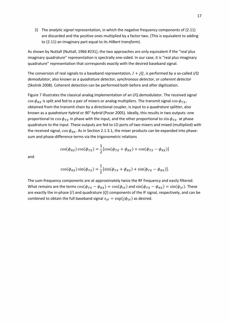
Figure 7 illustrates the classical analog implementation of an I/Q demodulator. The received signal
is split and fed to a pair of mixers or analog multipliers. The transmit signal ,
obtained from the transmit chain by a directional coupler, is input to a quadrature splitter, also
known as a quadrature hybrid or 90° hybrid (Pozar 2005). Ideally, this results in two outputs: one
proportional to in phase with the input, and the other proportional to at phase
quadrature to the input. These outputs are fed to LO ports of two mixers and mixed (multiplied) with
the received signal, . As in Section 2.1.3.1, the mixer products can be expanded into phase-
sum and phase-difference terms via the trigonometric relations
( ) ( )
, ( ) ( )-
and
( ) ( )
, ( ) ( )-
The sum-frequency components are at approximately twice the RF frequency and easily filtered.
What remains are the terms ( ) ( ) and ( ) ( ). These
are exactly the in-phase ( ) and quadrature ( ) components of the IF signal, respectively, and can be
combined to obtain the full baseband signal ( ) as desired.

18
Figure 7 Simplified block diagram of an analog I/Q demodulator for a homodyne FMCW system. The received signal is applied to a 3-dB power splitter, the two outputs of which are applied to the RF ports of (double-balanced) mixers. The local oscillator (LO) ports are driven by two samples of the transmit signal, the two components being in phase quadrature. The resulting outputs from the mixers are low-pass filtered and digitized by analog-to-digital (A/D) converters to obtain the in-phase ( ) and quadrature ( ) representative of the received vector.
Although the classical analog I/Q demodulator provides a clear example of how baseband
conversion can be implemented, in most modern systems I/Q demodulation is performed after
digitization. This has the advantage of avoiding so-called “I/Q mismatch” problems which hamper
the analog implementation (Pun, Franca et al. 2003). The flipside of this, however, is that digital I/Q
demodulators require a rate that is twice that of each of the A/D converters in Figure 7; in effect,
complex sampling requires real sampling at twice the rate. Given the high sample rates obtainable
with modern A/D converters, however, this is usually not a problem.
There are actually several techniques, referred to as “direct sampling digital coherent detection
techniques” (Pun, Franca et al. 2003), for performing baseband conversion after digitization, which
were developed in the early 1980s (Rice and Wu 1982; Waters and Jarrett 1982; Rader 1984). A
detailed discussion of these techniques is beyond the scope of this thesis; we will simply use the
result that the signal given by (2.9) can be obtained in baseband form.
2.1.4 Video signal
After quadrature sampling of the IF signal , a processor based on the fast Fourier transform (FFT)
resolves the beat frequency spectrum into frequency and range bins. Following Stove (Stove 1992),
we refer to the beat signal after frequency analysis as the video signal.
As explained in Section 2.1.3, the portion of the IF signal that is within the receiver bandwidth is a
pulse train with pulse length and pulse repetition interval . Since the IF signal is periodic with
period , its target range information can be obtained from the Fourier transform of a single
pulse:
splitter
quadrature
splitter
A/D
A/D
TX out
RX in
from transmitter
in-phase
component 𝐼
3 dB
directional
coupler
quadrature
component 𝑄
0° 90°
mixer low-pass
filter RF
LO
RF
LO
𝑓𝑠 ≥ 𝑓𝑏 𝑚𝑎𝑥
19
( ) ∫ ( ) ( )
(2.13)
where ( ) is given by (2.9). Here and throughout this thesis, functions represented by uppercase
letters are Fourier transforms of the functions represented by the corresponding lowercase letters.
Substituting (2.9) into (2.13), evaluating the Fourier integral, and taking its absolute value, we find
| ( )| ( ) ,( )( )- (2.14)
where ( ) is the normalized “sinc” function defined as
( ) ( )
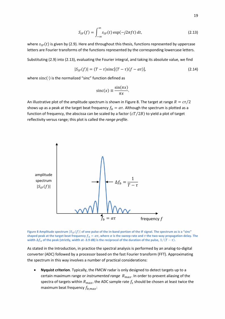
An illustrative plot of the amplitude spectrum is shown in Figure 8. The target at range ⁄
shows up as a peak at the target beat frequency . Although the spectrum is plotted as a
function of frequency, the abscissa can be scaled by a factor ( ⁄ ) to yield a plot of target
reflectivity versus range; this plot is called the range profile.
Figure 8 Amplitude spectrum | ( )| of one pulse of the in-band portion of the IF signal. The spectrum as is a “sinc” shaped peak at the target beat frequency , where is the sweep rate and the two-way propagation delay. The width of the peak (strictly, width at -3.9 dB) is the reciprocal of the duration of the pulse, ( )⁄ .
As stated in the Introduction, in practice the spectral analysis is performed by an analog-to-digital
converter (ADC) followed by a processor based on the fast Fourier transform (FFT). Approximating
the spectrum in this way involves a number of practical considerations:
Nyquist criterion. Typically, the FMCW radar is only designed to detect targets up to a
certain maximum range or instrumented range . In order to prevent aliasing of the
spectra of targets within , the ADC sample rate should be chosen at least twice the
maximum beat frequency :
Δ𝑓𝑏
𝑇 𝜏
frequency 𝑓
amplitude
spectrum
|𝑆𝐼𝐹(𝑓)|
𝑓𝑏 𝛼𝜏
20
≥ (2.15)
In order to prevent out-of-band noise from folding back into the target spectrum, the beat
signal is typically passed through an anti-aliasing filter, which is a low-pass filter with a cutoff
frequency between the maximum beat frequency and the Nyquist frequency .
ADC interval. As explained in Section 2.1.3, during the initial seconds of each sweep, a
portion of the beat signal for targets within the instrumented range is outside the bandwidth
of the ADC. This interval is usually omitted by delaying the sampling by seconds from
the beginning of each sweep, or alternatively by setting the samples collected during the
initial to zero {Adamski, 2000 #24}. As a result, the spectral width of a ‘point’ target is
( )⁄ for all targets within the instrumented range.
Sidelobe apodization. The beat signal spectrum ( ) given by (2.14) has the characteristic
‘sinc’ shape as predicted by Fourier theory. The range side lobes in this case are only 13.3 dB
lower than the main lobe, which is not satisfactory as it can result in the occlusion of small
nearby targets as well as introducing clutter from the adjacent lobes into the main lobes. To
counter these undesirable effects, a window function (Harris 1978) is usually applied to the
sampled IF signal prior to FFT frequency estimation. In our simulation in Chapter 0, we
employ a Hamming window with a highest sidelobe level of -43 dB.
These practical aspects are of importance in explaining our simulation in Chapter 09.
To summarize, we have analyzed the generation and spectral analysis of the beat signal in
mathematical detail for ideal, linear frequency sweeps. In the following section, we investigate how
this process is affected if the sweeps are nonlinear – in particular, if they are perturbed by sinusoidal
frequency sweep nonlinearity.
2.2 The effect of sinusoidal nonlinearity in the frequency sweep This section presents an analysis describing the effects on the range resolution of homodyne linear
FMCW radar of sinusoidal nonlinearities in the frequency sweep. Our discourse follows the analyses
of Richter (Richter, Jensen et al. 1973), Griffiths (Griffiths 1991; Griffiths and Bradford 1992), and
Piper (Piper 1995).
2.2.1 Analytical development
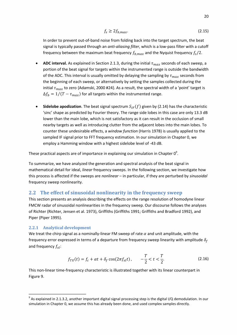
We treat the chirp signal as a nominally-linear FM sweep of rate and unit amplitude, with the
frequency error expressed in terms of a departure from frequency sweep linearity with amplitude
and frequency :
( ) ( )
(2.16)
This non-linear time-frequency characteristic is illustrated together with its linear counterpart in
Figure 9.
9 As explained in 2.1.3.2, another important digital signal processing step is the digital I/Q demodulation. In our
simulation in Chapter 0, we assume this has already been done, and used complex samples directly.
21
Figure 9 Time-frequency characteristics of a linear chirp (blue line) and a non-linear chirp (red curve). The linear chirp on the interval , - has a center frequency , duration , chirp rate , and frequency deviation (or ‘bandwidth’) . The non-linear chirp is
The phase of the transmitted signal is obtained by integrating the instantaneous angular
frequency in accordance with (2.4). Arbitrarily setting at (there is no
loss of generality here), we thus have the relation
( ) ∫ ( )
(2.17)
Inserting the expression (2.16) for into (2.17), we find
( ) (
) ( ) (2.18)
where is the “modulation index” of the transmitted chirp, i.e., its maximum phase
error.
The phase of the beat signal is given by (cf. (2.8))
( ) ( ) ( ) (2.19)
where is the target transit time as defined by (2.6). Inserting (2.18) into (2.19) yields
( ) (
) [ ( ) ( ( ))] (2.20)
or, using trigonometric identities to factorize the IF phase error term,
( ) (
) ( ) 0 .
/1 (2.21)
The baseband dechirped signal with envelope ( ) is therefore given by (cf. (2.9)):
𝑡
𝑓𝑇𝑋
𝑓𝑠𝑙
𝛿𝑓
𝑓𝑐
𝑇 𝑇
𝛼𝑇 linear chirp
non-linear chirp
22
( ) ( ) , ( )-
( ) 0 . 0 .
/1/1
(2.22)
where ( ⁄ ) is a constant phase term and
( ) (2.23)
is the “modulation index”, or maximum phase error, of the IF signal.
The expression (2.22) is recognizable from narrowband phase modulation theory. It can be
expanded as
( ) ( ) , ( )- { 0 .
/1
0 .
/1 }
(2.24)
Now, if we assume that the peak phase error is small, i.e.,
(2.25)
then only the first two terms of the expansion in (2.24) are significant. Thus the baseband dechirped
signal is approximately
( ) ( ) , ( )- {
0 .
/1
0 .
/1} (2.26)
which is the distortionless point-target response, plus a pair of sidelobes, or paired echoes, at .
The amplitude of each of these sidebands is .
2.2.1.1 Limit of long-wavelength phase errors
For long-wavelength phase errors such that the sidelobe ripple period is much larger than the target
transit time, i.e.,
(2.27)
(2.23) is well approximated by
(2.28)
where is the angular ripple frequency. Thus, for long-wavelength phase errors, the
modulation parameter in the beat signal increases linearly with the target transit time , and
hence with target range. Physically, we can say that for delays which are small compared to the
wavelength of the phase error, the transmitted and received phase errors ‘cancel out’10.
10
This is in contrast to conventional pulse compression radars, in which the ‘paired echo’ effect is independent of target range {Klauder, 1960 #20}. As a result, requirements on frequency sweep linearity can be considerably less stringent for FMCW radar than for LFM pulse compression radar, as noted by Griffiths {Griffiths, 1991 #36}.
23
2.2.1.2 General phase errors
In the preceding discussion, we considered a sinusoidal phase error. Here, we argue that the above
analysis can be extended to general phase errors.
A general phase error can be written in the form
( ) ( )
(2.29)
The error frequency ( ) can be expanded as a Fourier series:
( )
∑ [ (
) (
)]
1
(2.30)
where
∫ (
) ( )
∫ (
) ( )
(2.31)
Now, the constant term in (2.30) has only the effect of changing the center frequency of
the chirp, and since the center frequency is present in the beat signal phase only in the constant
phase term , this term has no effect on the amplitude spectrum of the beat signal.
Thus, neglecting the constant frequency term and integrating (2.30), we find that the phase
error ( ) is given by
( ) ∫ ( )
∑[
(
)
(
)]
1
(2.32)
(Here we have omitted a constant phase term which also has no effect on the range profile).
The phase error in the IF signal, , is the difference between the transmitted phase error
and its version delayed by :
( ) ( ) ( ) (2.33)
Inserting (2.32) into (2.33), subtracting term by term, and applying trigonometric identities as
before, we find
( ) ∑ .
/ 6
4
.
/5
4
.
/57
1
(2.34)
Now, a little thought shows that if we substitute (2.34) for the single-tone phase error
( ( )) in (2.22) and expand the factor ( ) as a Taylor series, then the
higher-order terms can be neglected as long as is small compared to unity. A sufficient
condition for this is that the amplitudes of the frequency errors are much smaller than the sweep
repetition frequency, i.e.,

24
(2.35)
In this case, the target beat spectrum consists of a superposition of ‘paired echoes’ spaced at
multiples of the sweep repetition frequency, , from the desired target beat signal.
In short, within small-angle approximations for the phase error, the ‘paired echoes’ associated with
the harmonics of the phase error merely superpose. Hence, an algorithm that compensates the
‘paired echoes’ for a chirp perturbed by sinusoidal phase errors and is linear should also work for
general phase errors, provided that these errors are sufficiently small. The derivation of such phase
error compensation algorithm is the subject of the next chapter.
25
3 An algorithm for compensating the effect of phase errors on the
FMCW beat signal spectrum In this chapter, we present a novel algorithm for compensating the effect of phase errors on the
FMCW beat signal spectrum by digital post-processing of the beat signal. Given amount of effort that
is currently put into making chirps linear, the existence of this algorithm is a very significant in the
field of FMCW ranging, and could render such elaborate chirp linearization methods obsolete.
This chapter is organized in three sections. In Section 3.1, we discuss similar algorithms that were
devised by others, and highlight the differences with our approach. In Section 3.2, we establish some
mathematical preliminaries – namely the quadratic phase filter and the Fresnel transform – which
will allow us to describe the algorithm more succinctly. In Section 3.3, we present a flow chart
describing the algorithm. In Section 3.4, we present an analytical derivation of the algorithm for
temporally infinite chirps, and show that the algorithm is exact in this case. In Section 3.5, we apply
the algorithm to finite chirps, and show that it remains approximately valid for chirps with large
time-bandwidth product and for which the phase error function contains only low frequencies.
3.1 Prior work A signal processing method was devised, apparently independently, by Burgos-Garcia et al. (Burgos-
Garcia, Castillo et al. 2003) and Meta et al. (Meta, Hoogeboom et al. 2006; Meta, Hoogeboom et al.
2007) to compensate for non-linearities in the frequency sweep (or equivalently, phase errors in the
phase) of FMCW signals. (Actually, the system described in (Burgos-Garcia, Castillo et al. 2003) is a
heterodyne time-domain pulse compression radar instead of a homodyne FMCW radar, but the
results can be applied to the latter case). The algorithm, which operates directly on deramped data,
corrects non-linearity effects for the whole range at once, and is computationally efficient.
Burgos-Garcia et al. and Meta et al. present the algorithm in a slightly different form, which is also
different from the one described here. In particular (as we will explain in more detail in Section 3.4),
1. In the last step of the algorithm described by Burgos-Garcia et al. (Burgos-Garcia, Castillo et
al. 2003), the phase error function in the receive signal, which they call ( ), is used
directly to cancel the residual phase error after removal of the transmitted errors and range
deskew. This is based on their stated assumption that the beat signal from the th target is a
narrowband signal centered at the frequency . Our derivation shows that this
assumption is not necessary, and that a skew-filtered version of the phase error function can
be used in the case that the beat signal is not narrowband11.
2. The algorithm described by Meta (Meta, Hoogeboom et al. 2006) does use a filtered version
of the phase error function in the last step. However, this version is a Fresnel transform of
the phase error function, whereas we believe it should be an inverse Fresnel transform12.
11
The author initiated a private e-mail correspondence with Mr. Burgos-Garcia, but unfortunately he was not at liberty to discuss the details of the algorithm under the terms of his project contract with the Spanish defense company Indra EWS. 12
The author also e-mailed Mr. Meta about this, but unfortunately he was too busy to study the derivation. Interestingly, an international an international patent application was submitted for this technique (Meta 2007), but at the time of writing is deemed to be withdrawn.
26
Moreover, (Burgos-Garcia, Castillo et al. 2003) and (Meta, Hoogeboom et al. 2006) use heuristic
arguments to justify the steps, and no formal proof of the algorithm was given. Our analytical
derivation in Section 3.4 is thus a novel contribution to the literature on this subject.
3.2 Mathematical preliminaries The key component of the phase error compensation (PEC) algorithm to be described is the
quadratic phase filter (QPF). As a prelude to our presentation of the algorithm, here we first discuss
the properties of this filter, as well as an integral transform called the Fresnel transform associated
with it (Gori 1994; Papoulis 1994).
3.2.1 The quadratic phase filter
A QPF is an all-pass system with quadratic phase. We denote by ( ) its impulse response and by
( ) its transfer function:
( ) √ ( ) ( ) 4
5 (3.1)
where the double arrow ( ) denotes a Fourier transform pair, and the time and frequency domains
are identified by the arguments and , respectively. Note that since neither ( ) nor ( ) is
square-integrable, this Fourier transform pair should be interpreted in the generalized sense as the
limit as of the Fourier transform of the complex Gaussian beam ( ( ) ), where
and are real parameters (Papoulis 1977).
The QPF is a dispersive filter which introduces a group delay proportional to the frequency. Group
delay is a measure of the time delay of the amplitude envelope of a sinusoidal component; it is in
general different from the phase delay, which is the time delay of the phase. The group delay of a
constant-modulus filter ( ) , ( )- is given by
( )
(3.2)
Thus, the group delay ( ) of the QPF given by (3.1) is
( )
(3.3)
Hence, the group delay of a QPF is linearly proportional to the frequency. (Incidentally, the group
delay of a QPF is the inverse function of the instantaneous frequency of its impulse response:
( ) . This result does not hold in general, but holds here because ( ) is a so-called
‘asymptotic’ signal (Boashash 1992)).
3.2.2 The Fresnel transform
The Fresnel transform with chirp parameter of a function ( ), denoted ( ) here, is by definition
the output of a QPF with input ( ):
( ) √ ∫ ( ) , ( ) -
( ) ( ) (3.4)
where the asterisk ( ) denotes the convolution product. The inversion formula reads
27
( ) √ ∫ ( ) , ( ) -
( ) ( ) (3.5)
so that the inverse transform simply equals the Fresnel transform with parameter .
Let us denote by ( ) the Fourier transform of a function ( ). From the definition (3.4) and the
convolution theorem, it follows that the Fourier transform ( ) of ( ) equals
( ) ( ) 4
5 (3.6)
It is also useful to investigate an asymptotic limit of the Fresnel transform. Based on the limit
(Papoulis 1977)
√ ( ) ( ) (3.7)
where ( ) denotes the Dirac delta function, it follows that in the limit the Fresnel transform
of a function approaches the function itself, i.e.,
( ) ( ) (3.8)
The Fresnel transform manifests itself several areas of signal and image processing, including pulse
compression, fiber-cable communications and dispersion, and Fresnel diffraction and optical filtering
(Papoulis 1994). Here, it will allow us to give a concise description of the PEC algorithm.
3.3 Description of the phase error compensation algorithm Suppose the transmitted signal is perturbed by a phase error ( ). We assume that ( ) is known
(its estimation is discussed in Chapter 0), and define the phase error function
( ) , ( )- (3.9)
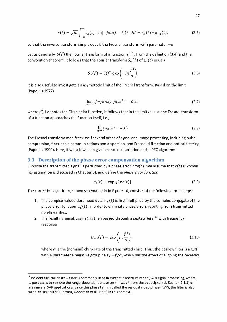
The correction algorithm, shown schematically in Figure 10, consists of the following three steps:
1. The complex-valued deramped data ( ) is first multiplied by the complex conjugate of the
phase error function, ( ), in order to eliminate phase errors resulting from transmitted
non-linearities.
2. The resulting signal, ( ), is then passed through a deskew filter13 with frequency
response
( ) 4
5 (3.10)
where is the (nominal) chirp rate of the transmitted chirp. Thus, the deskew filter is a QPF
with a parameter a negative group delay , which has the effect of aligning the received
13
Incidentally, the deskew filter is commonly used in synthetic aperture radar (SAR) signal processing, where its purpose is to remove the range-dependent phase term from the beat signal (cf. Section 2.1.3) of relevance in SAR applications. Since this phase term is called the residual video phase (RVP), the filter is also called an ‘RVP filter’ (Carrara, Goodman et al. 1995) in this context.
28
non-linearities in time14. (In the parlance of Section 3.2.2, is the inverse Fresnel
transform of ).
3. Finally, the deskewed signal ( ) is multiplied by the Fresnel transform ( ) of the
phase error function ( ). convolution product ( ) of the phase error function ( )
with a skew filter with an impulse response ( ), the frequency response ( ) of which
corresponds to the one in (3.10) with the sign of reversed.
The last step removes the received non-linearities to obtain the compensated signal ( ).
Figure 10 Schematic diagram of the phase error compensation algorithm. In the first step, the intermediate frequency (IF) signal ( ) is multiplied by the complex conjugate of the phase error function,
( ), to the remove the transmitted phase errors. The resulting signal ( ) is inverse Fresnel transformed by passing it through a deskew filter with impulse response ( ). This results in a signal ( ) in which the remaining phase errors, which emanate from the received signal, are aligned in time. Finally, ( ) is multiplied by a the Fresnel transform of the phase error function, ( ) ( ), to obtain the corrected IF signal .
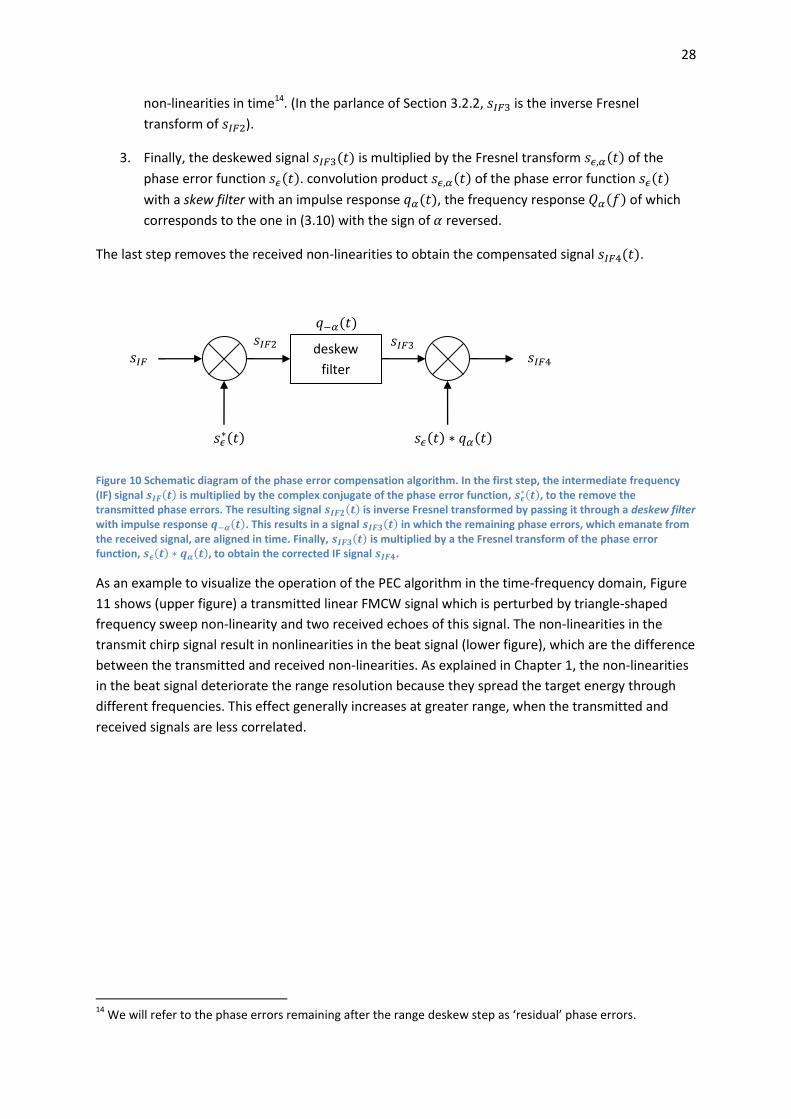
As an example to visualize the operation of the PEC algorithm in the time-frequency domain, Figure
11 shows (upper figure) a transmitted linear FMCW signal which is perturbed by triangle-shaped
frequency sweep non-linearity and two received echoes of this signal. The non-linearities in the
transmit chirp signal result in nonlinearities in the beat signal (lower figure), which are the difference
between the transmitted and received non-linearities. As explained in Chapter 1, the non-linearities
in the beat signal deteriorate the range resolution because they spread the target energy through
different frequencies. This effect generally increases at greater range, when the transmitted and
received signals are less correlated.
14
We will refer to the phase errors remaining after the range deskew step as ‘residual’ phase errors.
𝑞 𝛼(𝑡) 𝑠𝐼𝐹 𝑠𝐼𝐹
deskew
filter 𝑠𝐼𝐹 𝑠𝐼𝐹
𝑠𝜖 (𝑡) 𝑠𝜖(𝑡) 𝑞𝛼(𝑡)
29
Figure 11 Deramping of FMCW signals. The upper figure shows the instantaneous frequency of the transmitted chirp (solid line) and two received echoes (dashed lines). The lower figure depicts the corresponding two beat signals. The resulting frequencies of the beat signals are not constant, and their shape varies with target distance. The spreading of the beat signal in frequency is greater for the target response at larger distance than at the closer. (After (Meta, Hoogeboom et al. 2006)).
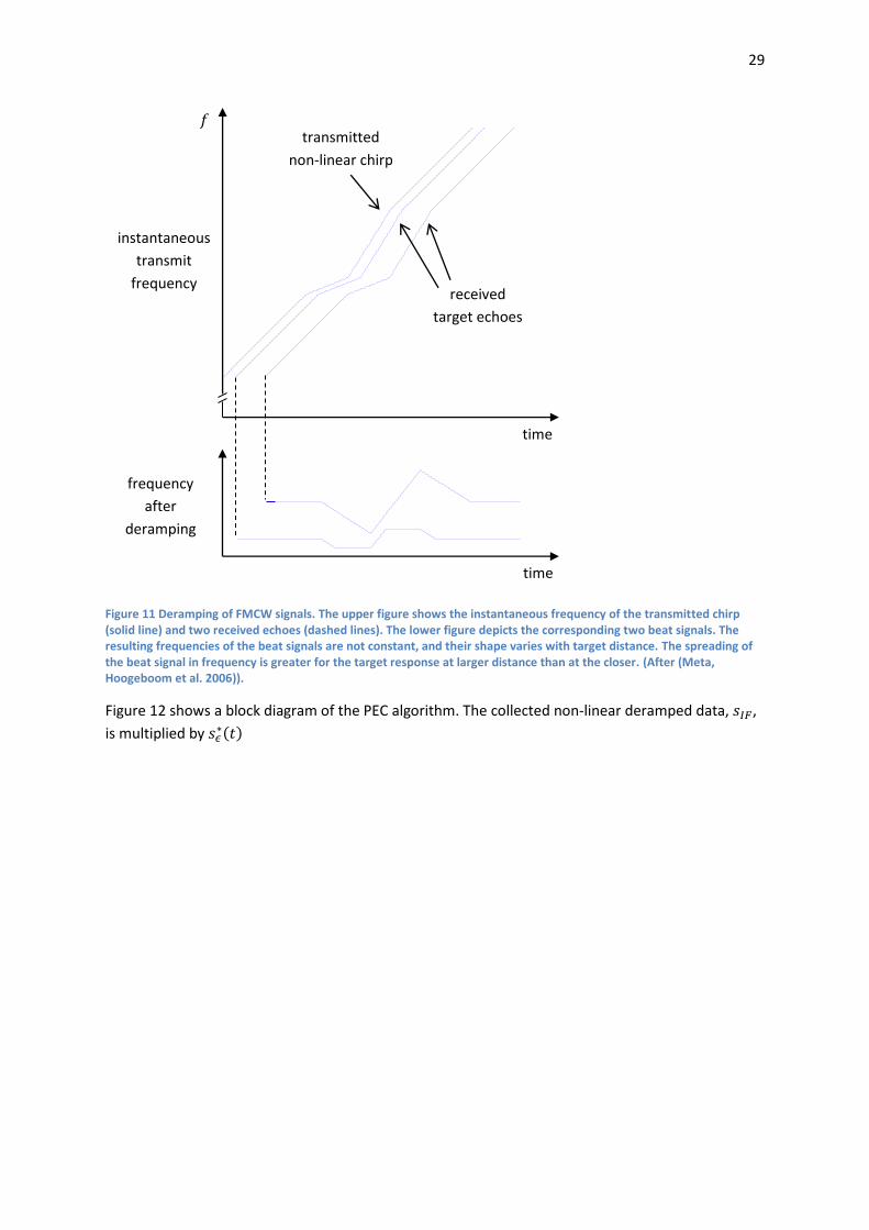
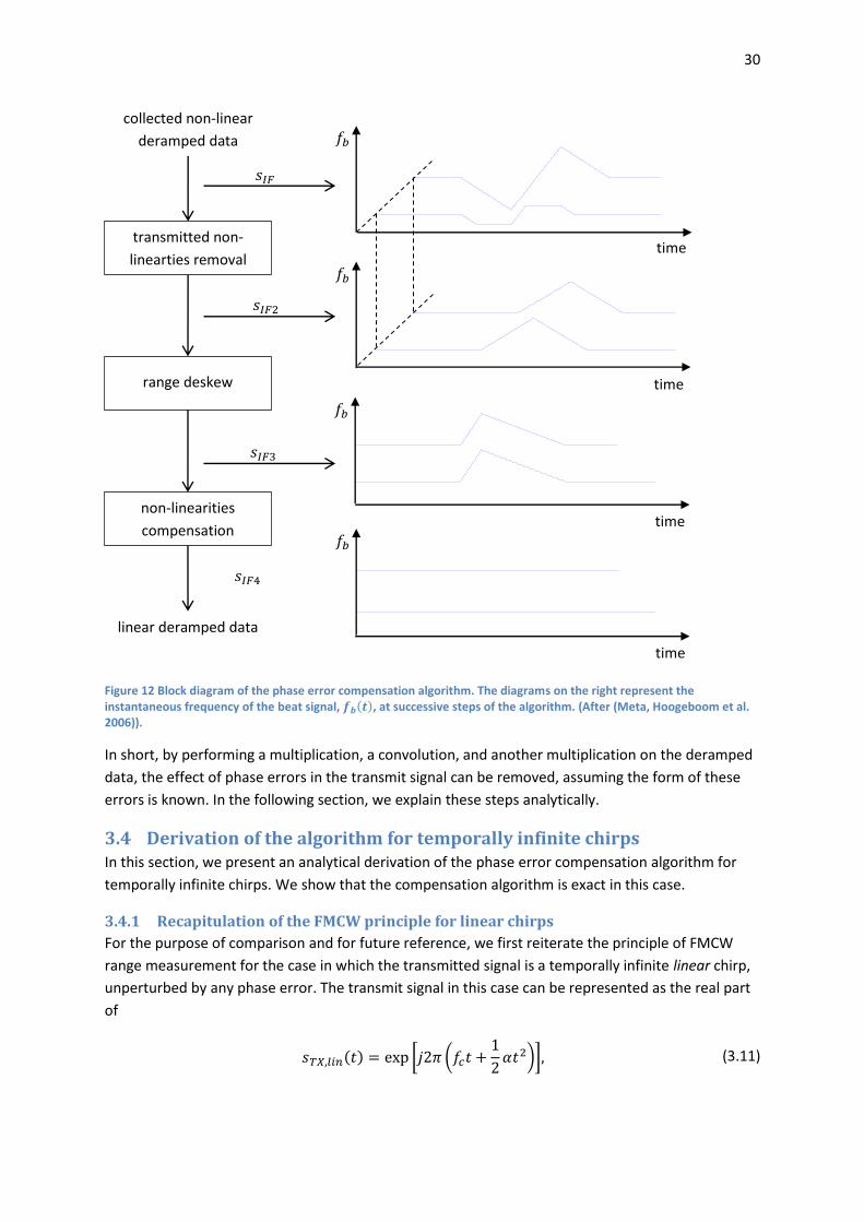
Figure 12 shows a block diagram of the PEC algorithm. The collected non-linear deramped data, ,
is multiplied by ( )
𝑓
time
transmitted
non-linear chirp
received
target echoes
time
frequency
after
deramping
instantaneous
transmit
frequency
30
Figure 12 Block diagram of the phase error compensation algorithm. The diagrams on the right represent the instantaneous frequency of the beat signal, ( ), at successive steps of the algorithm. (After (Meta, Hoogeboom et al. 2006)).
In short, by performing a multiplication, a convolution, and another multiplication on the deramped
data, the effect of phase errors in the transmit signal can be removed, assuming the form of these
errors is known. In the following section, we explain these steps analytically.
3.4 Derivation of the algorithm for temporally infinite chirps In this section, we present an analytical derivation of the phase error compensation algorithm for
temporally infinite chirps. We show that the compensation algorithm is exact in this case.
3.4.1 Recapitulation of the FMCW principle for linear chirps
For the purpose of comparison and for future reference, we first reiterate the principle of FMCW
range measurement for the case in which the transmitted signal is a temporally infinite linear chirp,
unperturbed by any phase error. The transmit signal in this case can be represented as the real part
of
( ) [ (
)] (3.11)
𝑓𝑏
𝑓𝑏
𝑓𝑏
𝑓𝑏
collected non-linear
deramped data
transmitted non-
linearties removal
range deskew
non-linearities
compensation
linear deramped data
𝑠𝐼𝐹
𝑠𝐼𝐹
𝑠𝐼𝐹
𝑠𝐼𝐹
time
time
time
time

31
where is the carrier frequency, is the time variable, and is the frequency sweep rate. Note that
in contrast to Eq. (2.2), there is no envelope factor ( ) in (3.11) since we are assuming that
the transmitted chirp is temporally infinite.
The received signal is a delayed version of the transmitted one (amplitude variations are not
considered in this derivation):
( ) [ ( ( )
( ) )] (3.12)
where is the round-trip time delay. In homodyne FMCW radar, the transmitted and received
signals are then mixed to generate the beat signal:
( ) ( ) ( )
[ (
)]
(3.13)
The beat signal is a sinusoidal signal with a frequency proportional to the round-trip time delay ,
and hence to the target range. The frequency information can be extracted using a Fourier
transform.
More precisely, except for a constant phase term, the Fourier transform ( ) of ( ) is a
Dirac delta function centered at the beat frequency :
( ) [ (
)] ( ) (3.14)
Of course in practice, the beat signal is observed over a finite interval, and the ideal response (3.14)
is convolved with the Fourier transform of the window function used.
3.4.2 Introduction of phase errors
When frequency nonlinearities are present in the transmitted signal, the signal modulation is no
longer an ideal chirp; the phase of the signal can be described as an ideal chirp plus a non-linear
error function ( ):
( ) 6 4
( )57
( ) ( )
(3.15)
The last term, accounting for systematic non-linearity of the frequency modulation, limits the
performance of conventional FMCW sensors. This phase term increases spectral bandwidth,
resulting in range resolution degradation and losses in terms of signal-to-noise ratio.
The beat signal is now represented by
( ) 6 4
( ) ( )57
( ) ( ) ( )
(3.16)
Equation (3.16) differs from (3.11) for the present of the last term ( ( ) ( )).
32
3.4.3 First step: removal of phase errors emanating from the transmitted signal
Assuming the non-linearity function ( ) is known (its estimation is discussed in Chapter 0), the
range-independent effect of the non-linear term in the beat frequency can be removed by the
following multiplication:
( ) ( ) ( )
6 4
( )57
(3.17)
The multiplication – which can because we have assumed that we have complex samples (both and
components) of the beat signal – removes the nonlinearities in the beat signal induced by the
nonlinear part of the transmitted signal. The residual nonlinearity term is present now only as a
result of the received signal. In order to remove this nonlinearity term with a single reference
function, any dependence on the time delay must be eliminated.
3.4.4 Second step: range deskew
To this end, the signal is passed through a quadratic phase filter ( ) with chirp parameter
– , where is the nominal chirp rate of the transmitted sweep; that is, is inverse Fresnel
transformed (or in the parlance of SAR signal processing, deskew-filtered) to obtain a signal :
( ) ( ) ( ) (3.18)
It will be shown that this convolution has the effect of aligning in time the phase errors emanating
from the received signal. This result can be derive d both in the frequency domain and in the time
domain. As an internal check on our results, we have done both, and present the derivations below.
3.4.4.1 Frequency-domain approach
In this approach, we determine the spectrum ( ) of the signal ( ) given by (3.18). Taking the
Fourier transform of (3.18), we obtain, by the convolution theorem and the definition of the deskew
filter transfer function (3.10),
( ) ( ) ( )
( ) 4
5
(3.19)
To evaluate ( ), we depart from the following expression for ( ) (which is easily seen by
comparison of (3.16) and (3.17)):
( ) ( ) ( ) (3.20)
Applying the convolution theorem to (3.20) yields
( ) ( ) * ( )+( ) (3.21)
where * +( ) denotes the Fourier transform with frequency variable . The first term, ( ), is
a Dirac delta function centered at the target beat frequency , as was shown in Eq. (3.14). The
second term can be expressed as
* ( )+( ) ( )
( ) (3.22)

33
where ( ) is the Fourier transform of the error signal ( ). Inserting (3.14) and (3.22) into (3.21)
yields
( ) { [ (
)] ( )} * ( )
( )+ (3.23)
Since convolution with ( ) shifts the spectrum to the right, but leaves it otherwise
unchanged, we have
( ) [ (
)] , ( ) -
, ( )- (3.24)
or, simplifying,
( ) ( ) 0
( )1
, ( )- (3.25)
where we have arranged the argument of the second complex exponential as an “incomplete
square”.
Inserting (3.25) into (3.19), and thus multiplying ( ) with the deskew filter transfer function
( ⁄ ), now “completes the square” in this complex exponential. We obtain
( ) ( ) 0
( ) 1
, ( )- (3.26)
Since the right hand side of (3.26) depends on the frequency through only, we can now use
the sifting property of the Dirac delta function “in reverse” to express ( ) as a convolution
product:
( ) * ( ) ( )+ 2 .
/
( )3 (3.27)
This expression is similar to the one for , Eq. (3.23), with one important difference: the second
factor of the convolution product no longer depends on the target transit time .
By the convolution theorem, the inverse Fourier transform of ( ), ( ), is given by
( ) 1* ( ) ( )+( ) 1 2 .
/
( )3 ( ) (3.28)
where 1* +( ) denotes the inverse Fourier transform with time variable and the bullet ( )
denotes ordinary multiplication. The first term is a pure sinusoid with frequency :
1* ( ) ( )+( ) , ( )- (3.29)
The second term in (3.28) represents the residual phase error after range deskew. Since ( ) is
the Fourier transform of ( ), this term can, using (3.6), immediately be seen to be the inverse
Fresnel transform of the complex conjugate of the error function , i.e.,
1 2 .
/
( )3 ( ) ( ) ( )
, ( ) ( )-
( )
(3.30)
34
where the second lines follows from the identity ( ) ( ). Hence, the residual phase error
function is the complex conjugate of the Fresnel transform of the error function .
Inserting (3.29) and (3.30) into (3.28), we find
( ) , ( )- ( ) (3.31)
Thus, after range deskew, the beat signal is an ideal sinusoid with frequency perturbed by a
phase error term ( ) which is independent of the target transit time .
3.4.4.2 Time-domain approach
The same result (3.31) can also be derived by a time-domain approach. Taking (3.18) as our starting
point and inserting the definition (3.1) of in the convolution integral, we find
( ) ( ) ( )
∫ 6 4
( )57
√ , ( ) -
(3.32)
By “completing the square” in the arguments of the complex exponentials, (3.32) can be written as
( ) , ( )- √ ∫ , ( ) - ( )
(3.33)
or, performing the substitution and some manipulations,
( ) , ( )-√ ∫ , ( ) - ( )
, ( )- 4√ ∫ , ( ) - ( )
5
, ( )- ( )
(3.34)
where ( ) is the Fresnel transform of the error signal ( ), in accordance with the definition
(3.4). This reproduces our result (3.31) obtained by the frequency-domain approach.
3.4.5 Third step: removal of residual phase errors
The last step of the phase error compensation is now clear: multiply by by to remove the
residual phase errors:
( ) ( ) ( )
, ( )- (3.35)
No error terms remain in the final, processed output, in which the residual video phase term
has also been removed. Therefore, spectral analysis of ( ) will yield the ideal target response.
To summarize, we have shown that if a temporally infinite chirp is perturbed by a general phase
error term ( ) , ( )-, then its corresponding IF signal ( ) can be converted into an
ideal response ( ) by three steps: removal of the transmitted phase errors by multiplication with
( ), range deskew by convolution with a quadratic phase filter ( ), and finally, removal of the
residual phase errors by multiplication with ( ) ( ) ( ).
35
3.4.6 Comparison with Meta’s algorithm
At this point, we note that our Equation (3.30) differs from the result obtained by Meta in his
Equation (10) of (Meta, Hoogeboom et al. 2006) by the presence of a minus sign in the complex
exponential. In other words, Meta uses an inverse Fresnel transform of the error function to obtain
the correction factor for the residual phase errors, whereas our formulation uses the Fresnel
transform15. As mentioned earlier, in a private correspondence with Mr. Meta he wrote that he
unfortunately did not have time to look into this discrepancy, but acknowledge that one of his
papers did contain a sign error. (This may, however, refer to the sign of the residual video phase in
equation (3) of (Meta, Hoogeboom et al. 2006), which also contains a sign error).
The author believes that the method described by Meta contains an error or typo, and that the
algorithm described in this thesis is correct. The fact that the two approaches – in the time and
frequency domain – to the derivation of the algorithm lead to the same result corroborates this
statement.
3.4.7 Narrowband IF signals: comparison with Burgos-Garcia’s algorithm
In the algorithm described by Burgos-Garcia et al. (Burgos-Garcia, Castillo et al. 2003), the phase
error ( ) itself is used for the removal of the residual phase errors in the last step, instead of its
Fresnel transform. This is based on their stated assumption that the IF signal is a narrowband signal,
which is equivalent to saying that the error signal spectrum ( ) contains only low frequencies.
Here, we verify that our algorithm reduces to Burgos-Garcia’s algorithm in this case. Specifically, we
will show that if ( ) contains only low frequencies, then
( ) ( ) (3.36)
That is, the Fresnel transform of the error function is approximately equal to the error function itself,
in which case our correction function for obtaining from reduces to the one given by
Burgos-Garcia et al. (Burgos-Garcia, Castillo et al. 2003). We will also derive a quantitative criterion
for the validity of (3.36).
To prove this statement, we adopt a frequency-domain approach. The Fourier transform ( ) of
( ) is given by (cf. (3.1))
( ) ( ) ( )
( ) 4
5
(3.37)
Expanding ( ) as a Taylor series, we obtain
( ) ( ) 6
7 (3.38)
15
Note that whether the Fresnel transform or its inverse is applied at a certain stage depends on how we define the phase of the IF signal. If we choose as we have here, then for positive transmitted chirps we obtain positive beat signals. However, we could have just as well chosen to define as the phase of the IF signal, in which case Fresnel transforms would be replaced by inverse Fresnel transforms and vice versa. In either case, however, two different Fresnel transforms would be used in the algorithm, whereas Meta uses Fresnel transforms of the same sign for both steps.

36
The Fresnel transform of the error function, ( ) is obtained by taking the inverse Fourier
transform of (3.38). The resulting series is called the moment expansion of the convolution product
(Papoulis 1977).
Now, the first term in (3.38) inverse Fourier transforms to ( ), which leads to the desired result
(3.36). Further, it can be seen that in order for the higher-order terms to have negligible
contributions, ( ) must be bandlimited and its maximum frequency component must be
much smaller than √ , i.e.,
√ (3.39)
If (3.39), then the higher-order terms in the square bracket expression of (3.38) will be much smaller
than unity will also increase with increasing order, so that only the zero-order term needs to be
maintained. Thus, if approximation (3.39) is satisfied, then our algorithm reduces to the one
described by Burgos-Garcia et al. (Burgos-Garcia, Castillo et al. 2003).
3.5 Application of the algorithm to finite chirps In the previous section, we derived the PEC algorithm for general phase errors ( ) and temporally
infinite chirps, and showed that it was exact in this case. The purpose of this section is to apply the
algorithm to finite chirps.
Actually, there are two varieties of the algorithm. One, discussed first in Section 3.5.1, is based on
the algorithm for narrowband IF signals discussed in Section 3.4.7. It is shown that this ‘narrowband
algorithm’ carries over directly to finite chirps provided the time-bandwidth product of the chirps is
large (i.e., ). The second variety of the algorithm holds for wideband IF signals, and is the
analog of the algorithm described and proved in Sections 3.4.1-3.4.6, and is described in Section
3.5.2. For the purpose of simplicity, we consider only sinusoidal phase errors (or, equivalently,
sinusoidal frequency sweep non-linearity).
infinite chirps finite chirps
wideband IF Sections 3.4.1-3.4.6 Section 3.5.1
narrowband IF Section 3.4.7 Section 3.5.2 Table 2 Sections in which different varieties of the compensation algorithm are discussed. Of course, the compensation algorithms for finite chirps are the ones which are of practical interest.
It is shown that the algorithm is still valid if the transmitted chirp has a large time-bandwidth
product .
3.5.1 Compensation algorithm for narrowband IF signals
Firstly, we attempt to carry over the derivation for temporally infinite chirps from Section 3.4 to a
temporally finite one of the form
( ) (
) 6 4
( )57 (3.40)
where is the sweep width, the center frequency, the sweep rate, and ( ) is a phase error
term in cycles (the phase error in radian is ( )), The finite chirp (3.40) is thus the same as the
infinite chirp (3.15) except for the pulse envelope ( ).
37
In analogy with Section 2.1.2, the received signal is simply delayed by the target transit time :
( ) (
) 6 4 ( )
( ) ( )57 (3.41)
Carrying over the steps in Section 2.1.3, the dechirped or intermediate frequency (IF) signal is now
( ) ( ) ( )
( ) 6 4
( ) ( )57
(3.42)
where ( ) is the IF signal envelope given by (2.10).
We wish to apply the phase error compensation algorithm to the finite chirp. The first step, removal
of the transmitted phase errors, can be applied just as in the temporally infinite case:
( ) ( ) ( )
( ) 6 4
( )57 (3.43)
Next, we apply the deskew filter to (3.43). Following the same steps as in the time-domain
derivation (Section 3.4.4.2), we find
( ) , ( )-√ ∫ ( ) , ( ) - ( )
, ( )-√ ∫ ( ) , ( ) - ( )
(3.44)
the second line of which differs from (3.34) for the presence of a factor ( ) in the convolution
integral. As a result, the integral is not independent of as in the case of temporally infinite chirps.
We can still derive an approximate compensation algorithm, however, if we assume that the IF
signal is narrowband as in Section 3.4.7. The integral in (3.44) can be seen to be the inverse Fresnel
transform of the function ( ) ( ):
√ ∫ ( ) , ( ) - ( )
* ( ) ( )+ ( ) (3.45)
In Section 3.4.7, the its was shown that Fresnel transform of a function is approximately equal to the
function itself if the function contains only low frequencies, such that its maximum frequency
component is much less than √ . It is easily seen that the same holds for the inverse Fresnel
transform.
Let us consider the spectrum of the function ( ) ( ). Since it is the convolution of the spectra
of ( ) and ( ), its maximum frequency component will be the sum of the maximum
frequency components of ( ) and ( ). Thus sum will be much less than √ if the
respective maximum frequency components of ( ) and ( ) are individually much less than
√ .
Now, ( ) is a rectangular analysis window of duration , as illustrated in Figure 13(a). Its
amplitude spectrum is a therefore a “sinc” function with peak-to-null distance ( )⁄ , as shown
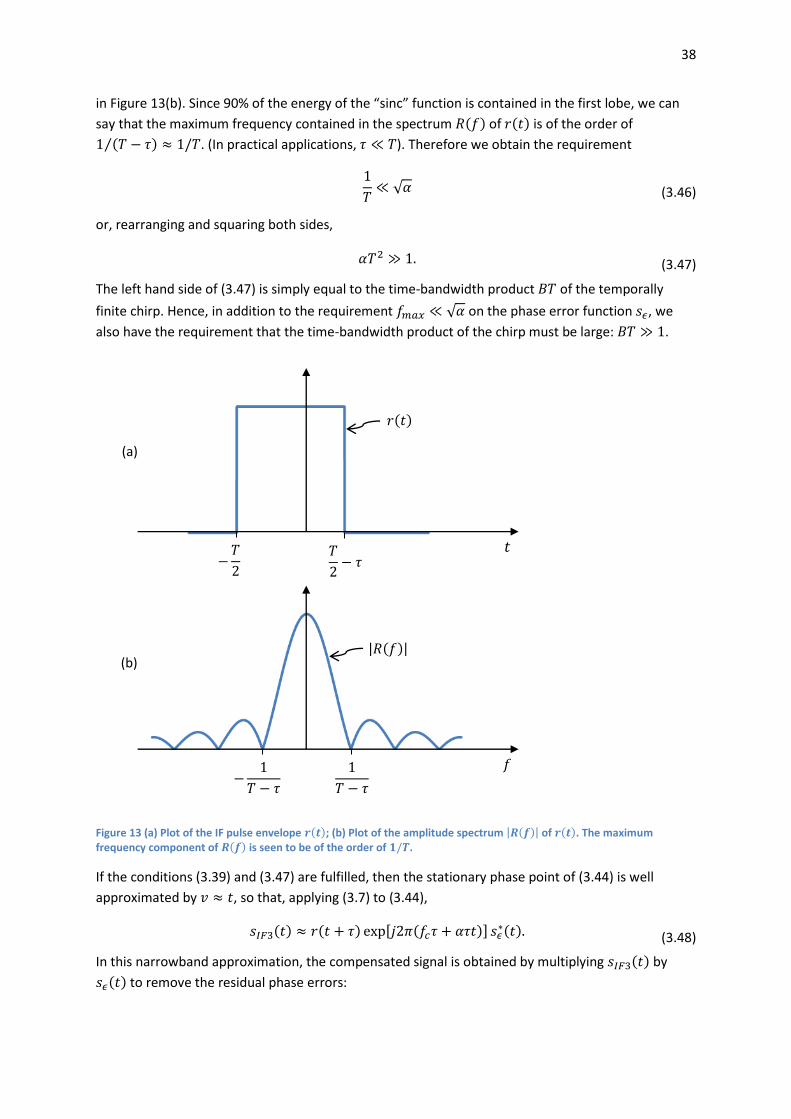
38
in Figure 13(b). Since 90% of the energy of the “sinc” function is contained in the first lobe, we can
say that the maximum frequency contained in the spectrum ( ) of ( ) is of the order of
( )⁄ . (In practical applications, ). Therefore we obtain the requirement
√ (3.46)
or, rearranging and squaring both sides,
(3.47)
The left hand side of (3.47) is simply equal to the time-bandwidth product of the temporally
finite chirp. Hence, in addition to the requirement √ on the phase error function , we
also have the requirement that the time-bandwidth product of the chirp must be large: .
Figure 13 (a) Plot of the IF pulse envelope ( ); (b) Plot of the amplitude spectrum | ( )| of ( ). The maximum frequency component of ( ) is seen to be of the order of .
If the conditions (3.39) and (3.47) are fulfilled, then the stationary phase point of (3.44) is well
approximated by , so that, applying (3.7) to (3.44),
( ) ( ) , ( )- ( ) (3.48)
In this narrowband approximation, the compensated signal is obtained by multiplying ( ) by
( ) to remove the residual phase errors:
𝑟(𝑡)
|𝑅(𝑓)|
𝑓
𝑇 𝜏
𝑇 𝜏
𝑇
𝑇
𝜏
𝑡
(b)
(a)

39
( ) ( ) ( )
( ) , ( )- (3.49)
In short, the approximate compensation method for narrowband IF signals described in Section 3.4.7
remains valid for finite chirps with large time-bandwidth products.
3.5.2 Application to sinusoidal phase errors
In the previous section, we essentially applied the stationary phase approximation to the deskew
filtering convolution integral (3.45), and assumed that the stationary point was not affected by
( ) ( ). However, if contains sufficiently high frequencies, the stationary point will change.
3.5.2.1 Characterization of the phase error function
To illustrate this effect, we assume the phase error ( ) is sinusoidal, and has the form (cf. Section
2.2)
( ) ( ) (3.50)
where is the phase error amplitude (in radian) and is the sidelobe ripple frequency. The
corresponding error signal ( ) is given by
( ) , ( )- , ( )- (3.51)
Since ( ) is periodic with period , it can be expressed as a Fourier series. It turns out
that (Carson 1922)
( ) ∑ ( ) ( )
(3.52)
where ( ) denotes the th order Bessel function of the first kind, defined as
( )
∫ ( )
(3.53)
The first four Bessel functions are illustrated graphically in Figure 14.

40
Figure 14 Bessel functions. (After (Klauder 1960)).
As seen from Figure 14, for small, we have the following approximations:
( ) 1( ) ⁄ ( )
(3.54)(a) (3.54)(b) (3.54)(c)
The approximations apply when (Klauder 1960)
(3.55) Further, using the identity
( ) ( ) ( ) (3.56)
we find that the error function ( ) can be approximated by
( )
, ( ) ( )- (3.57)
(Note that, similarly to Section 2.2, (3.57) can also be obtained by expanding the exponential in
(3.51) as a MacLaurin series, retaining only the first two terms, and using Euler’s theorem to express
the sine in terms of complex exponentials). In our subsequent calculations, we will assume a small-
amplitude phase error (i.e., ) and invoke the approximation (3.57).
3.5.2.2 Removal of the transmitted non-linearities
In the first step of the phase error compensation method, the transmitted linearities ( ) are
removed:
𝐽 (𝑥)
𝐽1(𝑥)
𝑥 ⁄
𝐽 (𝑥)
𝐽 (𝑥)
𝑥
41
( ) ( )
( ) ( ) ( )
( ) (3.58)
Inserting the small-angle approximation (3.57) into (3.58), we obtain
( ) ( )
. 1 /
[
( ( ) ( ))]
( ) ( ) ( ) (3.59)
where is the ‘main’ signal at the desired beat frequency :
( ) ( ) .
1 /
(3.60)
is ‘lower sidelobe’ with amplitude at frequency :
( )
( )
4( ) ( ) 1 5
(3.61)
and is an ‘upper sidelobe’ with amplitude at frequency :
( )
( )
4( ) ( ) 1 5
(3.62)
Thus, is found to consist of a ‘main’ signal at the desired beat frequency with amplitude unity
and two ‘paired echoes’ at with amplitude .
Note that has sidelobes with amplitudes , whereas the original IF signal has sidelobe
levels , where for long-wavelength phase errors ( ), . Thus, for long-
wavelength phase errors, the sidelobes in are actually higher than those in by a factor .
(Of course, is just an intermediate result; it is the sidelobe level in that ‘counts’).
3.5.2.3 Deskew filtering
In the second step of the compensation algorithm, we pass through a deskew filter to obtain a
third beat signal, :
( ) ( ) ( ) (3.63)
where (cf. (3.1))
( ) √ ( ) (3.64)
The output ( ) consists of three terms, ( ), ( ), and ( ) corresponding to the
three terms ( ), ( ), and ( ) of the input. We proceed to calculate these respective
terms, invoking the stationary phase approximation.
The output corresponding to the ‘main’ IF signal is
42
( ) √ .
1 /
∫ ( ) ( )
√ ( ) ∫ ( ) ( )
( ) ( )
(3.65)
where the approximation in the last step,
√ ( ) (3.66)
is valid for chirps with large time-bandwidth product,
(3.67)
and is justified by the same reasoning as in Section 3.5.1. (Note, however, that in this case we do not
have the additional condition √ , since there is no error function in the integrand of the
second line of (3.65)). Thus, comparing (3.65) with (3.61), we see that the deskew filter shifts the
envelope ( ) of ( ) backwards in time by seconds and imparts a phase shift of radians
to its carrier.
In a similar fashion, we obtain for the deskew-filtered lower sidelobe
( )
4( )
1 5
√ ∫ ( ) ( )( )
( ( ) )√ ∫ ( )
. .
/
/
‘Completing the square’ in the complex exponential in the integrand, we find
( )
4 ( )
1
5√ ∫ ( )
.
/
(3.68)
Applying the stationary phase approximation to (3.68)
( )
(
) 4 ( )
1
5 (3.69)
Thus, comparing (3.69) with (3.61), we see that the deskew filter shifts envelope ( ) of the lower
sidelobe of ( ) backwards in time by seconds ( seconds less than the ‘main’
signal) and acquires a phase shift of ( ) ⁄ radians to its carrier.
In an analogous fashion, we find for the upper sidelobe
( )
(
) 4 ( )
1
5 (3.70)
Thus, comparing (3.70) with (3.62), we see that the deskew filter shifts envelope ( ) of the lower
sidelobe of ( ) backwards in time by seconds ( seconds more than the ‘main’
signal) and acquires a phase shift of ( ) radians to its carrier.
Finally, adding the contributions (3.65), (3.69), and (3.70), we find

43
Finally, adding the contributions (3.65), (3.69), and (3.70), we find
( ) ( ) ( ) ( )
( ) ( )
(
) 4 ( )
1
5
(
) 4 ( )
1
5
(3.71)
Thus, the deskew-filtered signal ( ) comprises three terms, each offset slightly in both frequency
an time.
It is interesting to reflect on how the terms in (3.71) an be derived in a simpler fashion. Recall that
the transfer function of the deskew filter is given by
( ) .
/ , ( )- (3.72)
The envelopes, ( ), of ( ), ( ), and ( ) are delayed by the filter group delay,
(3.73)
evaluated at their respective frequencies , , and . As for the complex exponential
phase factors of ( ), ( ), and ( ), these are multiplied by the deskew filter
frequency response ( ) evaluated at these frequencies.
3.5.2.4 Restriction to an interval not affected by the finite nature of the chirp
On the interval , ⁄ ⁄ ⁄ ⁄ -, the envelopes of the three terms in (3.71) are all
equal to unity, and we have
( ) ( ) 6
( )7
( ) 6
( )7
(3.74)
Thus on this limited interval the signal is (to within the stationary phase approximation) the same as
if the chirp were temporally infinite.
3.5.2.5 Removal of the residual phase errors
In order to perform the next step of the phase error compensation algorithm, we compute
( ) ( ) ( ) (3.75)
where ( ) is the ‘skew’ filter with transfer function and frequency response
( ) √ ( ) .
/ ( ) (3.76)
Note that in the sign of is reversed with respect to the transfer function ( ) of the ‘deskew’
filter.
With the error function given by (3.57), it can be shown that
44
( )
( )
( )
(3.77)
Multiplying (3.74) and (3.77) and neglecting terms in , we find
( ) ( ) 6
( )
( )7
(3.78)
Now, provided that
√ (3.79)
the exponential terms in the square brackets in (3.78) will be close to unity, whence the second and
third terms in square brackets in (3.78) and we obtain
( ) ( )
(3.80)
It is important to note that the interval in (3.80) on which the compensated output is obtained is
shorter, by , than the interval on which it would be observed if there were no sinusoidal phase
error. Physically, this is because deskew filter applies different group delays to each original ‘paired
echo’, so that the ‘paired echoes’ at the output of the filter have less temporal overlap. This effect
could be of importance in our simulations, as we discuss in Section 4.5.

45
4 Simulation In this chapter, we simulate a signal processor implementing the phase error compensation
algorithm in order to verify the results derived in Chapter 3. The key part of the algorithm is the
deskew filter. Following Eichel et al. (Eichel 2005), we implement the filter in the frequency domain
using the frequency sampling method.
This chapter is organized as follows. In Section 4.1, we give an overview of the digital
implementation of the phase error compensation algorithm. In Section 4.2, we describe the
implementation of the digital deskew filter, and test it against a known exact solution. Finally, in
Section .., we present the full algorithm.
4.1 Digital implementation of the phase error compensation method The digital implementation of the phase error is illustrated in Figure 15. The input to the algorithm is
are samples of the coherently detected intermediate frequency (IF) signal, which appears as a finite
array of complex numbers, , -. This array is multiplied, element-by-element, with the sampled
values of the complex conjugate of the error function, , -, to remove phase errors emanating
from the transmitted signal. The thus obtained array , - is passed through a digital deskew filter,
described in Section 4.2, to obtain an output array , - in which the residual phase errors from
the received signal are time-aligned. Finally, , - is multiplied element-by-element with the
residual phase error function , - to remove the residual phase errors.
Figure 15 Digital implementation of the phase error compensation method.
The crucial part in the algorithm is the digital deskew filter to time align the phase errors in the
received echoes. Because it is a dispersive filter, the output is translated and ‘spread’ in time. This
calls for a different approach to the digital filter design than that used for frequency-selective finite
impulse response (FIR) filters commonly discussed in the literature (Oppenheim, Schafer et al. 1999),
which can be made to have linear phase.
4.2 Implementation of the deskew filter by the frequency sampling
method We implement the digital deskew filter using the frequency sampling method. This includes the
steps of performing the FFT on the deramped data, multiplying the result of the FFT on a sample-by-
sample basis with a pre-computed and pre-stored deskew vector, and performing the inverse FFT.
An artifact that commonly occurs in frequency sampling is time-domain aliasing, which is analogous
to the frequency-domain aliasing phenomenon in spectral estimation. In order to prevent time-
𝑠𝐼𝐹 ,𝑛- 𝑠𝐼𝐹 ,𝑛- digital
deskew filter 𝑠𝐼𝐹,𝑛- 𝑠𝐼𝐹
𝑠𝜖 ,𝑛- 𝑠𝜖 𝛼,𝑛-
46
domain aliasing from corrupting the filter output, the frequency sample spacing must be chosen
sufficiently small. This, in turn, requires that the FFT on the deramped data be performed after
padding it with a sufficient number of zeroes.
The organization of this section is as follows. In Subsection 4.2.1, we discuss the phenomenon of
time-domain aliasing in a general setting. In Subsection 4.2.2, we quantify the number of FFT points
required to prevent time-domain aliasing in a digital deskew filter implementation. Subsequently,
we describe the FFT implementation of the steps described in Section 4.1: approximation of the
spectrum of the input signal (Subsection 4.2.3), multiplication of the thus obtained approximation by
the exact deskew filter frequency response (Subsection 4.2.4), and using the thus obtained
frequency samples to approximate the filter output on a desired interval (Subsection 4.2.5). Finally,
in Subsection , we put the results of Subsections 4.2.3-4.2.5 together to
4.2.1 The frequency sampling method and time-domain aliasing
Consider the ideal case that a continuous-time input16 ( ) is passed through a deskew filter with
frequency response ( ). The continuous-time output ( ) in this case is given by the inverse
Fourier transform of ( ) ( ), i.e.,
( ) ∫ ( ) ( )
(4.1)
Now suppose we approximate this integral by a Riemann sum to obtain an approximate output ( ):
( ) ∑ ( ) ( ) ( )
(4.2)
where is the frequency sample spacing. For sufficiently small, we would expect ( ) ( );
we derive the form of the error presently.
The Riemann sum (4.2) can be expressed in the form of an inverse Fourier transform as follows:
( ) ∫ [ ∑ ( )
] ( ) ( )
(4.3)
The expression between square brackets in (4.3) represents a train of Dirac delta functions in the
frequency domain spaced Hertz apart, each with a gain of Hertz. The multiplication of the
convolution kernel ( ) ( ) by this impulse train effects the conversion of the inverse Fourier
integral (4.1) into the Reimann sum (4.2).
It can be shown (Bracewell 1986) that the inverse Fourier transform of the expression in square
brackets in (4.3) is a train of Dirac delta functions in the time domain with spacing seconds and
a gain of unity:
16
For the sake of generality and brevity, we use and here to denote the deskew filter input and output, respectively. (In the implementation of the phase error compensation algorithm, the deskew filter is actually used twice: once per sweep (‘on-line’) to compute from , and once beforehand (‘off-line’) to compute from . The general output and input thus represents either one of these pair of signals).
47
∑ ( )
∑ (
)
(4.4)
Thus, applying the convolution theorem to (4.3) and substituting (4.1) and (4.4), the Riemann sum
( ) can be expressed as
( ) ( ) ∑ (
)
∑ (
)
(4.5)
where we have used the “sifting property” of the Dirac delta function in the second step (Bracewell
1986). Hence, the output will consist of a periodic repetition of the desired output ( ) with period
. It follows that in order to prevent the aliases from overlapping each other, the duration of
( ) must be smaller than .
4.2.2 Number of FFT points required to prevent time-domain aliasing
Now suppose that the input ( ) is sampled at a rate , and complex samples are collected over a
period . Suppose that these samples are used to approximate the spectrum ( ) of ( )
on the Nyquist interval ( ).
Consider the effect of applying the deskew filter with frequency response ( ) to the input ( ).
As mentioned earlier, the filter has a group delay of ( ) . Therefore, the frequency
component at will experience a delay of , whereas the one at will experience one
of . This difference will cause the input pulse to widen by the amount . So the width of the
output will be
(4.6)
Now, if we extend the FFT operation from to points, then the frequency spacing will be
(4.7)
In order to prevent the time-domain aliases from overlapping each other, we must have
or, inserting (4.6) and (4.7) and rearranging,
(
) (4.8)
Using the fact that , (4.8) can alternatively be expressed as
(4.9)
Therefore, in order to prevent time-domain aliasing, the number of FFT points must be chosen
larger than the sum of the number of samples and the quantity , where is the sampling
frequency and the chirp rate of the quadratic phase filter. (This criterion can be relaxed somewhat
48
if the input signal is oversampled, i.e., does not contain frequency components all the way up to its
Nyquist frequency).
4.2.3 Approximating the input signal spectrum
As indicated in Section 4.1, the first step in the frequency sampling implementation of the deskew
filter is to approximate the spectrum ( ) of the input signal ( ).
Regarding the input as time-limited to the sweep interval , -, we want to find the
spectrum of a time-limited function ( ):
( ) ∫ ( )
(4.10)
Defining the grid points
(4.11)
where
(4.12)
is the sampling period, we approximate the integral in (4.10) as a left-hand Riemann sum17, to obtain
an approximation ( ) of the exact spectrum ( ):
( ) ∑ ( )
1
( ) ∑ ( )
1
(4.13)
where we have substituted (4.11) to obtain the second line.
The function ( ) given by (4.13) is at this point still a continuous function of frequency, . A digital
signal processor, however, can only output an array of sampled values of this function, due to its
discrete nature. We choose to evaluate ( ) on the following array of points:
(
) (4.14)
where
17 The Riemann sum ( ) given by (4.13) is only a first-order accurate approximation of the exact signal
spectrum ( ). Several methods for obtaining higher-order accuracy have been proposed in the literature
(see, for example, (Press, Teukolsky et al. 2007)). Although higher-order accuracy would be desirable in a real-
time implementation of the PEC algorithm, in this thesis we are interested in providing a “proof of principle”,
and therefore we have chosen to use the simpler, first-order accurate formula (4.13).

49
(4.15)
is the sampling frequency. The array (4.14) thus represents a partition of the Nyquist interval
( ) into sub-intervals, so that the frequency sample spacing is as required.
Evaluating the approximation ( ) given by (4.13) on the grid points given by (4.14), we find
( )
( ) ∑( ) ( ) (
)
1
(4.16)
For , the sum in (4.16) this has the standard form of an -point FFT as
implemented by MATLAB®, for example.
Mathematical symbol MATLAB symbol
( ) X
( ) x
f
, - n
, - k
N, NFFT
Table 3 Mathematical expressions and their corresponding MATLAB symbols.
Identifying the mathematical expressions in (4.16) with MATLAB symbols as in Table 3, the spectrum
( ) can be approximated at the points given by (4.14) by the following line of MATLAB code:
X=T/N*(-1).^(f*T).*fft(x.*(-1).^n,NFFT); (4.17)
A short explanation of the code is as follows. In MATLAB, the symbols “.*” and “.^” denote the array
(i.e., element-by-element) multiplication and array power operations, respectively. Further, the
operation fft(s,NFFT) on an array s produces the NFFT-point discrete Fourier transform (DFT)
of that array. In our case in which the FFT length is larger than the array length (NFFT>N), this
means that the so the input array s is padded with NFFT-N trailing zeroes prior to performing the
DFT.
4.2.4 Multiplication by the exact deskew filter frequency response
Thus, the digital spectrum ( ) of the input signal is approximated at discrete points on the
Nyquist interval ( ). This is multiplied by the deskew filter transfer function evaluated at
these points to obtain the output ( ):
( ) ( ) ( )
.
/
(4.18)
This gives an approximation of the output on the Nyquist interval ( ).
In MATLAB code, this is implemented as follows:
Y=X.*exp(1j*pi*f.^2/alpha); (4.19)
Here fs = N/T is the sampling rate, and alpha (‘mathematical’ symbol: ) is the chirp rate of the
deskew filter.

50
4.2.5 Inverse Fourier transform of the spectrum of the output
Next, we wish to take the inverse Fourier transform of ( ) to obtain an approximate output ( ):
( ) ∫ ( ) ( )
(4.20)
Approximating this integral by a Riemann sum, we obtain an approximation ( ) of ( ):
( )
∑ ( ) ( )
1
(4.21)
Inserting the expression for the , equation (4.14), into (4.21) yields
( ) ( )
∑ ( ) (
)
1
(4.22)
Evaluating ( ) at the time points given by (4.11), and again assuming that contains more than
one prime factor of 2, we find
( ) ( ) [
∑ ( )
( ) (
)
1
] (4.23)
The term between square brackets has the MATLAB form of a -point inverse DFT. Thus, the
filter output for is obtained by the following MATLAB code:
y=fs*(-1).^(fs*t).*ifft((-1).^(k*N/NFFT).*Y,NFFT);
y=y(1:N); (4.24)
The first line in (4.24) computes an -point inverse DFT. The first points of this represent the
desired output.
4.2.6 Implementation of the deskew filter as a MATLAB function
The results of the previous subsections can be combined to a concise MATLAB code. After combining
the steps described above, the output of the digital deskew filter with chirp rate on input sampled
at a rate is found to depend on the dimensionless parameter
(4.25)
A listing of our MATLAB function, deskew, is given below in nine lines of code.
function y=deskew(x,A) 1 N=length(x); 2 NFFT=2^nextpow2(N+1/abs(A)); 3 n=0:N-1; 4 k=0:NFFT-1; 5 X=exp(1j*pi*N*(-1/2+k/NFFT)).*fft(x.*(-1).^n,NFFT); 6 Y=X.*exp(1j*pi*(-1/2+k/NFFT).^2/A); 7 y=exp(1j*pi*(N/2-k)).*ifft(Y.*exp(-1j*pi*k*N/NFFT),NFFT); 8 y=y(1:N); 9
51
A short explanation of the code is as follows. In line 3, we choose the number of FFT points as the
next power of 2 larger than ⁄ , as specified in Subsection 4.2.2. Lines 4 and 5
define the discrete-time indices n and k corresponding to the time samples and frequency
samples , respectively. Line 6 is an implementation of (4.16) in which a factor has been omitted,
since this factor later cancels against a factor which would be required in line 8. Line 7 is an
implementation of (4.19), in which the factor in the definition of the is combined with the
factor to . Lines 8 and 9 are an implementation of (4.24), where a pre-factor has been
omitted as explained earlier.
4.2.7 Test of the deskew filter for a known, exact output
We have tested the deskew filter for the case in which the IF signal is the linear IF signal, not
perturbed by phase errors:
( ) ( ) 4 (
)5 (4.26)
The deskew filter output in this case is
( ) , ( )-√
6 4√ (
)5 4√ (
)57 (4.27)
A comparison of these two functions is shown below.

52
Figure 16 Real part of the input (blue line) and deskew filter output (red, green lines) for a time-bandwidth product of 100.
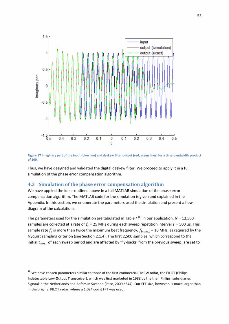
53
Figure 17 Imaginary part of the input (blue line) and deskew filter output (red, green lines) for a time-bandwidth product of 100.
Thus, we have designed and validated the digital deskew filter. We proceed to apply it in a full
simulation of the phase error compensation algorithm.
4.3 Simulation of the phase error compensation algorithm We have applied the ideas outlined above in a full MATLAB simulation of the phase error
compensation algorithm. The MATLAB code for the simulation is given and explained in the
Appendix. In this section, we enumerate the parameters used the simulation and present a flow
diagram of the calculations.
The parameters used for the simulation are tabulated in Table 418. In our application, = 12,500
samples are collected at a rate of = 25 MHz during each sweep repetition interval = 500 μs. This
sample rate is more than twice the maximum beat frequency, = 10 MHz, as required by the
Nyquist sampling criterion (see Section 2.1.4). The first 2,500 samples, which correspond to the
initial of each sweep period and are affected by ‘fly-backs’ from the previous sweep, are set to
18 We have chosen parameters similar to those of the first commercial FMCW radar, the PILOT (Philips
Indetectable Low Output Transceiver), which was first marketed in 1988 by the then Philips’ subsidiaries
Signaal in the Netherlands and Bofors in Sweden {Pace, 2009 #344}. Our FFT size, however, is much larger than
in the original PILOT radar, where a 1,024-point FFT was used.
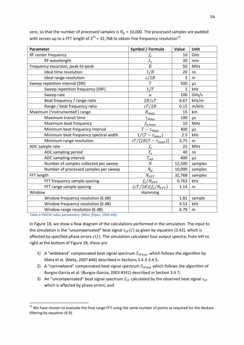
54
zero, so that the number of processed samples is = 10,000. The processed samples are padded
with zeroes up to a FFT length of 215 = 32,768 to obtain fine frequency resolution19.
Parameter Symbol / Formula Value Unit
RF center frequency 10 GHz
RF wavelength 30 mm
Frequency excursion, peak-to-peak 50 MHz
Ideal time resolution 20 ns
Ideal range resolution 3 m
Sweep repetition interval (SRI) 500 μs
Sweep repetition frequency (SRF) 2 kHz
Sweep rate 100 GHz/s
Beat frequency / range ratio 6.67 kHz/m
Range / beat frequency ratio 0.15 m/kHz
Maximum (‘instrumented’) range 15 km
Maximum transit time 100 μs
Maximum beat frequency 10 MHz
Minimum beat frequency interval 400 μs
Minimum beat frequency spectral width ( )⁄ 2.5 kHz
Minimum range resolution , ( )-⁄ 3.75 m
ADC sample rate 25 MHz
ADC sampling period 40 ns
ADC sampling interval 400 μs
Number of samples collected per sweep 12,500 samples
Number of processed samples per sweep 10,000 samples
FFT length 32,768 samples
FFT frequency sample spacing ⁄ 0.763 kHz
FFT range sample spacing ( ⁄ )( ⁄ ) 1.14 m
Window Hamming
Window frequency resolution (6 dB) 1.81 sample
Window frequency resolution (6 dB) 4.53 kHz
Window range resolution (6 dB) 6.79 m Table 4 FMCW radar parameters. (After {Piper, 1993 #4}).
In Figure 18, we show a flow diagram of the calculations performed in the simulation. The input to
the simulation is the “uncompensated” beat signal ( ) as given by equation (3.42), which is
affected by specified phase errors ( ). The simulation calculates four output spectra; from left to
right at the bottom of Figure 18, these are:
1) A “wideband” compensated beat signal spectrum , which follows the algorithm by
Meta et al. {Meta, 2007 #46} described in Sections 3.4.3-3.4.5;
2) A “narrowband” compensated beat signal spectrum which follows the algorithm of
Burgos-Garcia et al. {Burgos-Garcia, 2003 #341} described in Section 3.4.7;
3) An “uncompensated” beat signal spectrum calculated by the observed beat signal
which is affected by phase errors; and
19
We have chosen to evaluate the final range FFT using the same number of points as required for the deskew filtering by equation (4.9).

55
4) An “ideal” beat signal spectrum calculated from the ideal beat signal given by
(3.13).
The beat signals are windowed prior to performing the range FFT. Since the deskew filter effectively
translates the beat signal in time, different window functions are used for the compensated signals
( and ) and the uncompensated signals ( and ). The uncompensated signals use a
Hamming window with support on the interval , ⁄ ⁄ ). The compensated signals,
however, use a Hamming window shifted seconds to the left, which thus has support on the
interval , ⁄ ⁄ ).
Figure 18 Flow diagram of the simulation. The crossed circles represent multiplications, the “deskew” blocks represent deskew filtering, and the “ ” blocks represent (approximate) Fourier transformation. The remaining blocks represent
𝑠𝐼𝐹
deskew
𝑠𝜖
𝑠𝐼𝐹
𝑠𝐼𝐹
𝑠𝜖 deskew
𝑤𝐼𝐹
𝑠𝐼𝐹 𝑤 𝑠𝐼𝐹 𝑛
𝑤𝐼𝐹
𝑠𝐼𝐹 𝑙𝑖𝑛
𝑆𝐼𝐹 𝑤 𝑆𝐼𝐹 𝑆𝐼𝐹 𝑙𝑖𝑛 𝑆𝐼𝐹 𝑛
“wideband”
compensation
algorithm
“narrowband”
compensation
algorithm
uncompensated
IF signal ideal
IF signal
“compensated”
window
function
“uncompensated”
window function

56
names of arrays at various stages of the calculation. The colors of the bottom boxes correspond to the colors of the plots generated by the simulation (see Section 4.4).
An important aspect of the flow diagram shown above is that we have applied the deskew (not
skew) filter to the function in order to obtain remove the residual phase errors in the last step of
the “wideband” compensation algorithm. This corresponds to the algorithm as originally formulated
by Meta {Meta, 2007 #46}, and was found to give better results in our simulations for sinusoidal
phase errors in Section 4.4.1. However, it is at odds with our analytical derivations in Chapter 3. We
return to this point in Section 4.5. (Note that if the phase error function contains only low
frequencies such that (3.39) is satisfied, then either variety of the algorithm will work, since in this
case by virtue of (3.8)).
In the MATLAB code implementing the simulation, the phase error ( ) is specified on a separate
line as an in-line function. By changing this in-line function, we can apply the phase error
compensation algorithms to any phase error we like. The results for a number of phase errors are
described presently.
4.4 Results for cases of interest The MATLAB code described in Section 4.3 was used to simulate the performance of both the
“wideband” and the “narrowband” compensation algorithm for a number of cases of interest.
4.4.1 Sinusoidal phase errors
We have performed simulations using a sinusoidal phase error of the form (cf. (2.18))
( ) ( ) (4.28)
where represents the peak phase error (in radian), and the sidelobe ripple frequency. The
performance of the compensation algorithms depends on these parameters, as we show presently.
4.4.1.1 Low-frequency phase error ( √ )
First, we investigate the case in which the and √ . From the first condition, it can be
inferred from narrowband modulation theory that the maximum frequency component in ( ) is
approximately . Thus, the second condition, √ , amounts to condition (3.39), and
we the “narrowband” compensation algorithm to be effective as well as the “wideband” one. We
also note that for the parameters of our simulation, the time-bandwidth product is
, so that (3.47) for all cases simulated here.
With = 100 GHz/s as specified in Table 4, √ ≈ 316 kHz. We have chosen well below that, at
kHz, and have chosen = 0.1. The simulated range profiles with these parameters are
shown in Error! Reference source not found..
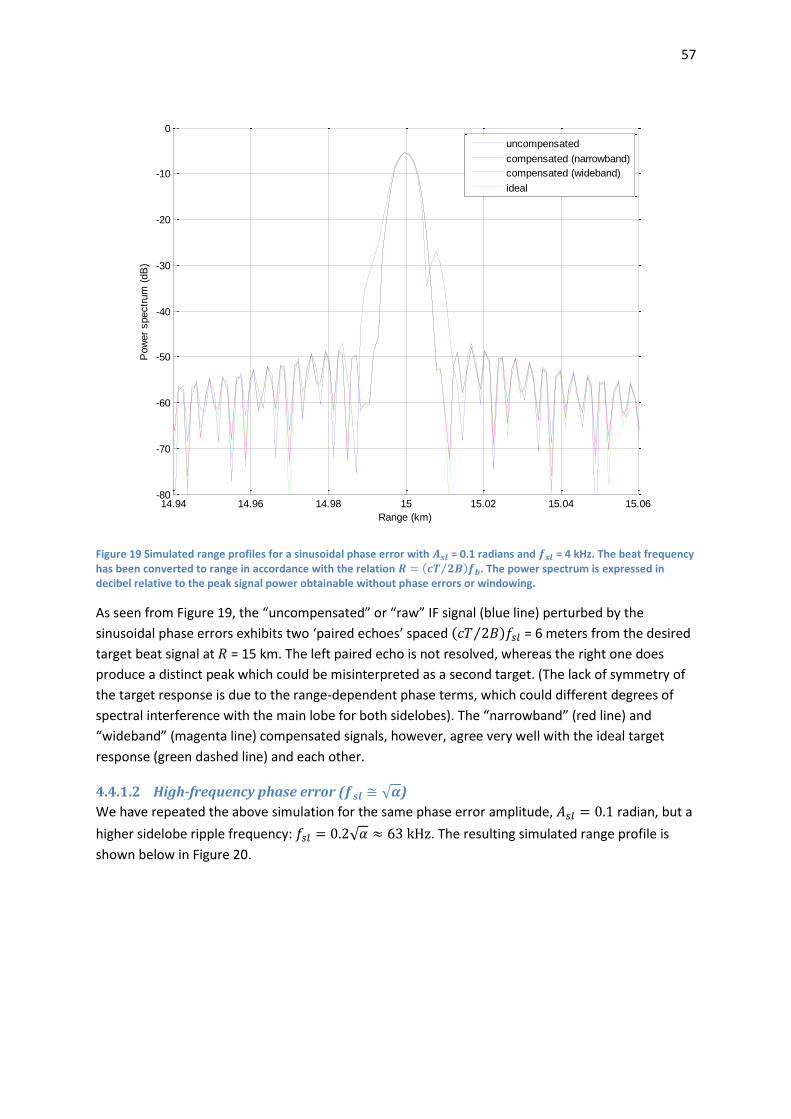
57
Figure 19 Simulated range profiles for a sinusoidal phase error with = 0.1 radians and = 4 kHz. The beat frequency has been converted to range in accordance with the relation ( ⁄ ) . The power spectrum is expressed in decibel relative to the peak signal power obtainable without phase errors or windowing.
As seen from Figure 19, the “uncompensated” or “raw” IF signal (blue line) perturbed by the
sinusoidal phase errors exhibits two ‘paired echoes’ spaced ( ⁄ ) = 6 meters from the desired
target beat signal at = 15 km. The left paired echo is not resolved, whereas the right one does
produce a distinct peak which could be misinterpreted as a second target. (The lack of symmetry of
the target response is due to the range-dependent phase terms, which could different degrees of
spectral interference with the main lobe for both sidelobes). The “narrowband” (red line) and
“wideband” (magenta line) compensated signals, however, agree very well with the ideal target
response (green dashed line) and each other.
4.4.1.2 High-frequency phase error ( √ )
We have repeated the above simulation for the same phase error amplitude, radian, but a
higher sidelobe ripple frequency: √ . The resulting simulated range profile is
shown below in Figure 20.
14.94 14.96 14.98 15 15.02 15.04 15.06-80
-70
-60
-50
-40
-30
-20
-10
0
Range (km)
Pow
er
spectr
um
(dB
)
uncompensated
compensated (narrowband)
compensated (wideband)
ideal
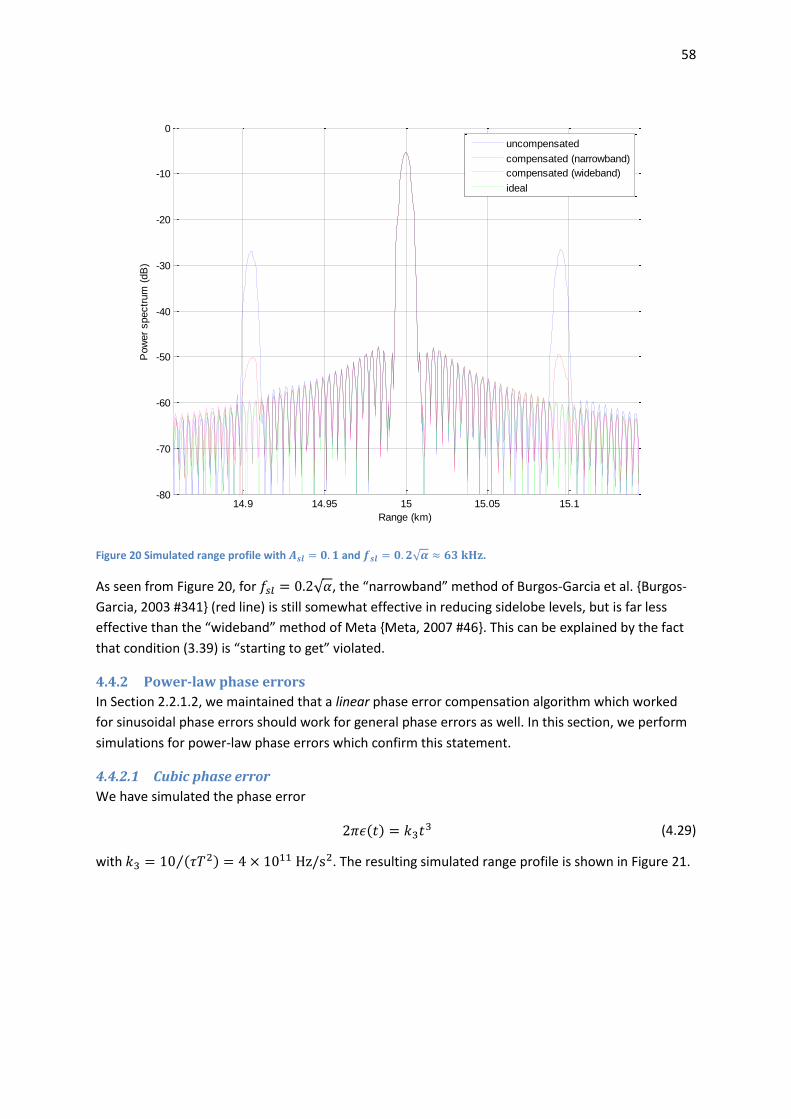
58
Figure 20 Simulated range profile with and √ .
As seen from Figure 20, for √ , the “narrowband” method of Burgos-Garcia et al. {Burgos-
Garcia, 2003 #341} (red line) is still somewhat effective in reducing sidelobe levels, but is far less
effective than the “wideband” method of Meta {Meta, 2007 #46}. This can be explained by the fact
that condition (3.39) is “starting to get” violated.
4.4.2 Power-law phase errors
In Section 2.2.1.2, we maintained that a linear phase error compensation algorithm which worked
for sinusoidal phase errors should work for general phase errors as well. In this section, we perform
simulations for power-law phase errors which confirm this statement.
4.4.2.1 Cubic phase error
We have simulated the phase error
( ) (4.29)
with ( )⁄ 11 . The resulting simulated range profile is shown in Figure 21.
14.9 14.95 15 15.05 15.1-80
-70
-60
-50
-40
-30
-20
-10
0
Range (km)
Pow
er
spectr
um
(dB
)
uncompensated
compensated (narrowband)
compensated (wideband)
ideal
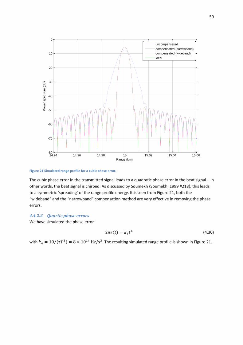
59
Figure 21 Simulated range profile for a cubic phase error.
The cubic phase error in the transmitted signal leads to a quadratic phase error in the beat signal – in
other words, the beat signal is chirped. As discussed by Soumekh {Soumekh, 1999 #218}, this leads
to a symmetric ‘spreading’ of the range profile energy. It is seen from Figure 21, both the
“wideband” and the “narrowband” compensation method are very effective in removing the phase
errors.
4.4.2.2 Quartic phase errors
We have simulated the phase error
( ) (4.30)
with ( )⁄ 1 . The resulting simulated range profile is shown in Figure 21.
14.94 14.96 14.98 15 15.02 15.04 15.06-80
-70
-60
-50
-40
-30
-20
-10
0
Range (km)
Pow
er
spectr
um
(dB
)
uncompensated
compensated (narrowband)
compensated (wideband)
ideal

60
Figure 22 Simulated range profile with quartic phase errors.
A quartic phase error in the transmitted signal gives rise to a cubic phase error in the beat signal.
Thus, the beat signal is nonlinearly chirped, which gives rise to the asymmetric point target response
shown above {Soumekh, 1999 #218}. Both the “wideband” and “narrowband” compensations are
again effective in this case.
4.5 Concluding remarks To summarize, we have simulated both the “wideband” and “narrowband” phase error
compensation algorithms, and found that “narrowband” algorithm provides effective compensation
of low-frequency phase errors, while the “wideband” algorithm also works well for high-frequency
phase errors.
In our implementation of the “wideband” algorithm, the suppression of ‘paired echoes’ was found to
be better if we applied a deskew filter to the phase error function , instead of a skew filter as
derived in Section 3.4, which is apparently at odds with our analytical development in Chapter 3.
This does not necessarily imply that our derivation is incorrect, however. As shown in Section 3.5.2,
if we apply a deskew filter to a time-limited phase-modulated signal (in our case, ), then due to
the different group delays of the ‘paired echoes’, the interval on which the deskew filter output
matches that for a temporally infinite phase-modulated signal is shorter than the duration of the
original signal. In other words, “edges” of the original interval are “contaminated” by artifacts due to
the time-limited nature of . However, in our simulations, we have not taken into account this
14.94 14.96 14.98 15 15.02 15.04 15.06-80
-70
-60
-50
-40
-30
-20
-10
0
Range (km)
Pow
er
spectr
um
(dB
)
uncompensated
compensated (narrowband)
compensated (wideband)
ideal
61
effect, and have performed the spectral analysis over the entire sweep period in all cases20. Further
work must be carried out to ascertain what the effect of the “contaminated edges” is.
20
In any case, the portion affected by this “contamination” is small; for example, for the parameters in the
example in Section 4.4.1.2 where √ , the relative group delay of the “upper and lower sidelobes” relative to the main target signal is only ≈ 0.63 μs, or 0.13% of the sweep period. However, the amplitudes of the remaining sidelobes after applying the phase error compensation algorithm with a skew filter in the last step is of the same order of magnitude.
62
5 Estimation of the phase errors In the development of the phase error compensation algorithm, it was assumed that the phase error
term ( ) was known. In this section, we overcome this assumption and describe how to estimate
( ) directly from the deramped data.
In Section 5.1, we review a known method of determining the error function using a reference delay.
5.1 Review of a known method using a reference delay One way to measure the phase error in linear frequency-modulated (LFM) radar systems, first
described by Withers {Withers, 1966 #389} and also applied by Meta {Meta, 2007 #364}, uses a
reference response with delay , which is usually implemented using a delay line. The IF signal
corresponding to this reference response is
( ) 6 4
( ) ( )57 (4.31)
For small delays, we can approximate the phase error in the IF signal as
( ) ( ) ( ) (4.32)
where ( ) denotes the derivative of ( ) with respect to time. This relation is also the basis of the
resampling methods to compensate frequency sweep non-linearity {Vossiek, 1998 #390}; in this
case, however, we require (4.32) to hold only for the reference delay , and not for every in the
range window of interest.
We thus obtain an estimate, ( ), for ( ) as follows:
( ) ( ) ( )
(4.33)
Integrating (4.33), we find a phase error estimate
( ) ∫ ( )
(4.34)
The constant phase is of no consequence for the power spectrum of the beat signal.
A problem with the ‘reference delay’ method is that we have two conflicting requirements. On one
hand, we would like to choose small, so that (4.32) yields a good approximation of the
derivative ( ). On the other hand, however, if is small, the differential phase error ( )
( ) is small, and could easily be swamped by stochastic phase errors. It would seem
advantageous to deduce ( ) by observing the beat signals for larger target delays, when the effects
of the phase errors are more conspicuous. Moreover, it seems intuitive that there is something to be
learned from how the phase errors develop with increasing .
5.2 Proposal of a novel method using ambiguity functions In this section, we propose a novel method for estimating the phase error in the transmit signal ( )
from the deramped data observed for different ranges.

63
If we consider the beat signal spectrum ( ) to be a function of as well, we can write it in the
form
( ) ∫ ( ) ( )
( ) (4.35)
Now, suppose that ( ) can be expressed as follows:
( ) ( ) ( ) (4.36)
where ( ) is called the waveform of the transmitted signal and its carrier frequency. Then (4.35)
has the form
( ) ( )∫ ( ) ( ) ( )
(4.37)
Defining ( ) ( ) ( ), this can be written as
( ) ∫ ( ) ( ) ( )
(4.38)
The function ( ) is called the ambiguity function of ( ). Thus, the problem of determining the
transmitted signal ( ) from the spectrum of the IF signal, ( ), is equivalent to that of
determining a function ( ) from its ambiguity function ( ).
The latter problem was discussed by Wilcox {Wilcox, 1991 #391}. An important aspect here, though,
is that not all functions of two variables ( and ) are ambiguity functions: the ambiguity functions
are a subspace of the space of all functions of two variables. (In fact, Wilcox shows that a basis for
the subspace of ambiguity functions ( ) can be obtained from the cross-ambiguity functions ofa
family of orthogonal basis functions for the space of waveforms, ( )). Wilcox also describes a
method to project a given function of two variables onto the space of ambiguity functions.
Now, consider a series of measurements ( ) from which we want to determine the waveform
( ) – and hence, the phase error function ( ). Suppose the measurements are perturbed by
other errors, which as stochastic errors or errors incurred in the receive signal chain, which are not
attributable to an error in the transmitted frequency sweep. These “other” phase errors generally do
not give rise to ambiguity functions, and will be “filtered out” when the measured data ( ) is
projected onto the space of ambiguity functions in order to determine ( ). Hence, we expect the
method of Wilcox to more robust in the presence of other sources of error.
Needless to say, more simulation work must be done to validate the ideas laid out above, which
unfortunately was no longer available within the period
64
6 Conclusions and discussion The nonlinearity of the frequency sweep is a limiting factor for the performance of linear FMCW
radars in many applications. In this thesis, we have studied methods devised by Burgos-Garcia et al.
{Burgos-Garcia, 2003 #341} and Meta et al. {Meta, 2007 #46} to compensate for such nonlinearities
by digital post-processing of the deramped signal.
To summarize, in this thesis we make the following accomplishments and contributions to
knowledge:
We derive the phase error compensation algorithm for “wideband” signals, and find a
discrepancy with the algorithm as originally presented by Meta {Meta, 2007 #46} in that in
our method, the phase error function ( ) is “skewed” (Fresnel transformed), to obtain the
correction function to remove the residual phase errors in the last step, whereas in Meta’s
algorithm ( ) is “deskewed” (inverse Fresnel transformed) for that purpose. We derive our
version of the algorithm in two different ways, one set in the frequency domain and one in
the time domain, and check it for a small-angle sinusoidal phase error.
We show that the algorithm of Meta, which is applicable for wideband IF signals, reduces to
the algorithm of Burgos-Garcia in the case of narrowband IF signals.
We simulate both algorithms, and shown that they are effective within their underlying
assumptions.
We propose a novel method for determining phase errors which, by projecting the IF signal
spectrum observed at different ranges onto the space of ambiguity functions for the
waveform of the transmitted signal, should provide more robust measurement of the
transmitted sweep nonlinearities in the presence of other sources of error.
The findings of this thesis could have major technological implications. The existence of these
algorithms means that transmitted frequency sweeps need not necessarily be linear, which in turn
means that all the hardware techniques devised for generating linear sweeps could become
obsolete.
Removing the requirement that sweeps must be linear also has major implications for electronic
warfare. If an intercept receiver knows what type of radar signals to expect (for example, linear
chirps), it can devise processing methods to increase its processing gain, reducing the processing
gain advantage of the FMCW radar and thereby jeopardizing the radar’s tactical advantage. If the
transmitted sweep no longer has to be linear, however, the ability of intercept receivers to achieve
such processing gain is reduced, and the low probability of intercept (LPI) property of FMCW radars
maintained.
65
Bibliography Adamy, D. (2001). EW 101: a first course in electronic warfare. Norwood, MA, Artech House. Adamy, D. (2004). EW 102: A Second Course in Electronic Warfare, Horizon House Publications, Inc. Barrick, D. E. (1973). FM/CW Radar Signals and Digital Processing. Beasley, P. and D. Lawrence (2006). Frequency Modulated Continuous Wave (FMCW) Radar Having Improved Frequency Sweep Linearity. Q. Ltd. Beasley, P. D. L. (2009). Coherent Frequency Modulated Continuous Wave Radar. U. S. P. Office. Beasley, P. D. L., A. G. Stove, et al. (1990). Solving the problems of a single antenna frequency modulated CW radar. Radar Conference, 1990., Record of the IEEE 1990 International. Boashash, B. (1992). "Estimating and interpreting the instantaneous frequency of a signal. I. Fundamentals." Proceedings of the IEEE 80(4): 520-538. Bracewell, R. N. (1986). The Fourier transform and its applications, McGraw-Hill. Brooker, G. M. (2005). Understanding Millimetre-Wave FMCW Radars. 1st International Conference on Sensing Technology. Palmerston North, New Zealand: 152-157. Burgos-Garcia, M., C. Castillo, et al. (2003). "Digital on-line compensation of errors induced by linear distortion in broadband LFM radars." Electronics Letters 39(1): 116-118. Caputi, W. J. (1971). "Stretch: A Time-Transformation Technique." Aerospace and Electronic Systems, IEEE Transactions on AES-7(2): 269-278. Carrara, W. G., R. S. Goodman, et al. (1995). Spotlight Synthetic Aperture Radar: Signal Processing Algorithms, Artech House. Carson, J. R. (1922). "Notes on the Theory of Modulation." Proceedings of the IRE 10(1): 57-64. Chen, V. C. and H. Ling (2002). Time-Frequency Transforms for Radar Imaging and Signal Analysis, Artech House. Cooley, J., P. Lewis, et al. (1967). "Application of the fast Fourier transform to computation of Fourier integrals, Fourier series, and convolution integrals." Audio and Electroacoustics, IEEE Transactions on 15(2): 79-84. Eichel, P. H. (2005). IFP V4.0: A Polar-Reformatting Image Formation Processor for Synthetic Aperture Radar, Sandia National Laboratories. Fuller, K. L. (1990). "To see and not be seen [radar]." Radar and Signal Processing, IEE Proceedings F 137(1): 1-10. Gori, F. (1994). Why is the Fresnel Transform So Little Known? Current Trends in Optics. J. C. Dainty, Academic Press.
66
Griffiths, H. D. (1990). "New ideas in FM radar." Electronics & Communication Engineering Journal 2(5): 185-194. Griffiths, H. D. (1991). The effect of phase and amplitude errors in FM radar. High Time-Bandwidth Product Waveforms in Radar and Sonar, IEE Colloquium on. Griffiths, H. D. and W. J. Bradford (1992). "Digital generation of high time-bandwidth product linear FM waveforms for radar altimeters." Radar and Signal Processing, IEE Proceedings F 139(2): 160-169. Gurgel, K. W. and T. Schlick (2009). Remarks on Signal Processing in HF Radars Using FMCW Modulation. International Radar Symposium IRS 2009. Hamburg, Germany: 63-67. Harris, F. J. (1978). "On the use of windows for harmonic analysis with the discrete Fourier transform." Proceedings of the IEEE 66(1): 51-83. Jakowatz, C. V., D. E. Wahl, et al. (1996). Spotlight-Mode Synthetic Aperture Radar: A Signal Processing Approach, Kluwer Academic Publishers. James, G. L. (2003). Geometrical Theory of Diffraction for Electromagnetic Waves, Peter Peregrinus Ltd. Keller, J. B. (1962). "Geometrical Theory of Diffraction." J. Opt. Soc. Am. 52(2): 116-130. Klauder, J. R., Price, A.C., Darlington, S., and Albersheim, W.J. (1960). "The Theory and Design of Chirp Radars." Bell. Syst. Tech. J. 39(4): 745-809. Levanon, N. and E. Mozeson (2004). Radar Signals, John Wiley & Sons. Meta, A. (2007). Frequency Modulated Continuous Wave Radar and Synthetic Aperture Radar. N. O. v. T.-N. O. (TNO) and E. B.V. Meta, A., P. Hoogeboom, et al. (2006). Range Non-linearities Correction in FMCW SAR. Geoscience and Remote Sensing Symposium, 2006. IGARSS 2006. IEEE International Conference on. Meta, A., P. Hoogeboom, et al. (2007). Signal processing for FMCW SAR, Ieee-Inst Electrical Electronics Engineers Inc. Meta, A., P. Hoogeboom, et al. (2007). "Signal Processing for FMCW SAR." Geoscience and Remote Sensing, IEEE Transactions on 45(11): 3519-3532. Morgan, G. D., P. D. Beasley, et al. (2006). Design considerations for a millimetric front-end for FMCW radar. MM-Wave Products and Technologies, 2006. The Institution of Engineering and Technology Seminar on. Nalezinski, M., M. Vossiek, et al. (1997). Novel 24 GHz FMCW front-end with 2.45 GHz SAW reference path for high-precision distance measurements. Microwave Symposium Digest, 1997., IEEE MTT-S International. Oppenheim, A. V., R. W. Schafer, et al. (1999). Discrete-time signal processing, Prentice-Hall. Pace, P. E. (2004). Detecting and classifying low probability of intercept radar, Artech House.
67
Papoulis, A. (1977). Signal Analysis, McGraw-Hill. Papoulis, A. (1994). "Pulse compression, fiber communications, and diffraction: a unified approach." J. Opt. Soc. Am. A 11(1): 11. Papoulis, A. (1994). "Pulse compression, fiber communications, and diffraction: a unified approach." J. Opt. Soc. Am. A 11(1): 3-13. Pichler, M., A. Stelzer, et al. (2003). Influence of Systematic Frequency-Sweep Non-Linearity on Object Distance Estimation in FMCW/FSCW Radar Systems. European Microwave Conference, 2003. 33rd. Piper, S. O. (1993). Receiver frequency resolution for range resolution in homodyne FMCW radar. Telesystems Conference, 1993. 'Commercial Applications and Dual-Use Technology', Conference Proceedings., National. Piper, S. O. (1995). Homodyne FMCW radar range resolution effects with sinusoidal nonlinearities in the frequency sweep. Radar Conference, 1995., Record of the IEEE 1995 International. Pozar, D. M. (2005). Microwave Engineering, John Wiley & Sons, Inc. Press, W. H., S. A. Teukolsky, et al. (2007). Computing Fourier Integrals Using the FFT. Numerical Recipes - The Art of Scientific Computing, Cambridge University Press. Pun, K. P., J. E. d. Franca, et al. (2003). Circuit Design for Wireless Communications - Improved Techniques for Image Rejection in Wideband Quadrature Receivers, Kluwer Academic Publishers. Rader, C. M. (1984). "A Simple Method for Sampling In-Phase and Quadrature Components." Aerospace and Electronic Systems, IEEE Transactions on AES-20(6): 821-824. Rice, D. W. and K. H. Wu (1982). "Quadrature Sampling with High Dynamic Range." Aerospace and Electronic Systems, IEEE Transactions on AES-18(6): 736-739. Richards, M. A., J. A. Scheer, et al. (2010). Principles of Modern Radar, SciTech Publishing, Inc. Richter, J. H., D. R. Jensen, et al. (1973). "New Developments in FM-CW Radar Sounding." Boundary-Layer Meterology 4: 179-199. Ross, R. A. and M. E. Bechtel (1968). "Scattering-Center Theory and Radar Glint Analysis." Aerospace and Electronic Systems, IEEE Transactions on AES-4(5): 756-762. Scheer, J. A. (1993). Coherent Radar Performance Estimation, Artech House. Sheehan, D. V. and H. D. Griffiths (1992). "The effect of pulse phase distortion on the height estimation of a radar altimeter." International Journal of Remote Sensing 13(17): 3303-3310. Skolnik, M. (2008). Radar Handbook, McGraw-Hill. Soumekh, M. (1999). Synthetic Aperture Radar Signal Processing with MATLAB Algorithms, John Wiley & Sons.

68
Stove, A. G. (1992). "Linear Fmcw Radar Techniques." Iee Proceedings-F Radar and Signal Processing 139(5): 343-350. Stove, A. G., A. L. Hume, et al. (2004). "Low probability of intercept radar strategies." Radar, Sonar and Navigation, IEE Proceedings - 151(5): 249-260. Strauch, R. G. (1976). Theory and Application of the FM-CW Doppler Radar. Department of Electrical Engineering. Boulder, University of Colorado. Ph.D. Waters, W. M. and B. R. Jarrett (1982). "Bandpass Signal Sampling and Coherent Detection." Aerospace and Electronic Systems, IEEE Transactions on AES-18(6): 731-736. Willis, N. J. and H. D. Griffiths (2007). Advances in Bistatic Radar, SciTech Publishing, Inc.
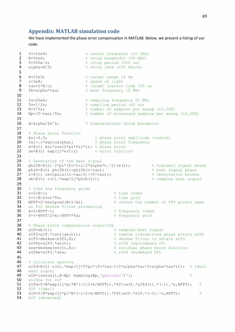
69
Appendix: MATLAB simulation code We have implemented the phase error compensation in MATLAB. Below, we present a listing of our
code.
fc=10e9; % center frequency (10 GHz) 1 B=50e6; % chirp bandwidth (50 MHz) 2 T=500e-6; % chirp period (500 us) 3 alpha=B/T; % chirp rate (100 GHz/s) 4 5 R=15e3; % target range 15 km 6 c=3e8; % speed of light 7 tau=2*R/c; % target transit time 100 us 8 fb=alpha*tau; % beat frequency 10 MHz 9 10 fs=25e6; % sampling frequency 25 MHz 11 Ts=1/fs; % sampling period (40 ns) 12 N=T/Ts; % number of samples per sweep (12,500) 13 Np=(T-tau)/Ts; % number of processed samples per sweep (10,000) 14 15 A=alpha/fs^2; % dimensionless chirp parameter 16 17 % Phase error function 18 Asl=0.5; % phase error amplitude (radian) 19 fsl=.1*sqrt(alpha); % phase error frequency 20 e=@(t) Asl*cos(2*pi*fsl*t); % phase error 21 se=@(t) exp(1j*e(t)); % error function 22 23 % Generation of the beat signal 24 phiTX=@(t) 2*pi*(fc*t+1/2*alpha*t.^2)+e(t); % transmit signal phase 25 phib=@(t) phiTX(t)-phiTX(t-tau); % beat signal phase 26 r=@(t) rectpuls((t-tau/2)/(T-tau)); % observation window 27 sb=@(t) r(t).*exp(1j*phib(t)); % complex beat signal 28 29 % Time and frequency grids 30 n=0:N-1; % time index 31 t=(-N/2+n)*Ts; % time grid 32 NFFT=2^nextpow2(N+1/A); % choose the number of FFT points same 33 as for deskew filter processing 34 k=0:NFFT-1; % frequency index 35 f=(-NFFT/2+k)/NFFT*fs; % frequency grid 36 37 % Phase error compensation algorithm 38 sIF=sb(t); % sampled beat signal 39 sIF2=sIF.*conj(se(t)); % remove transmitted phase errors sIF2 40 sIF3=deskew(sIF2,A); % deskew filter to obtain sIF3 41 sIF4n=sIF3.*se(t); % sIF4 (narrowband IF) 42 sea=deskew(se(t),A); % residual phase error function 43 sIF4w=sIF3.*sea; % sIF4 (wideband IF) 44 45 % Calculate spectra 46 sIFd=@(t) r(t).*exp(1j*2*pi*(fc*tau-1/2*alpha*tau^2+alpha*tau*t)); % ideal 47 beat signal 48 wIF=[zeros(1,N-Np) hamming(Np,'periodic')']; % 49 window for sIF 50 SIFd=T/N*exp(1j*pi*N*(-1/2+k/NFFT)).*fft(wIF.*sIFd(t).*(-1).^n,NFFT); % 51 SIF (ideal) 52 SIF=T/N*exp(1j*pi*N*(-1/2+k/NFFT)).*fft(wIF.*sIF.*(-1).^n,NFFT); % 53 SIF (observed) 54

70
wIF4=[hamming(Np,'periodic')' zeros(1,N-Np)]; % 55 window for sIF4 56 SIF4n=T/N*(-1).^(N*(-1/2+k/NFFT)).*fft(wIF4.*sIF4n.*(-1).^n,NFFT); % SIF4 57 (narrowband IF) 58 SIF4w=T/N*(-1).^(N*(-1/2+k/NFFT)).*fft(wIF4.*sIF4w.*(-1).^n,NFFT); % SIF4 59 (wideband IF) 60 61 % Convert to normalized decibel scale 62 SIFd_dB=20*log10(abs(SIFd)/(T-tau)); 63 SIF_dB=20*log10(abs(SIF)/(T-tau)); 64 SIF4n_dB=20*log10(abs(SIF4n)/(T-tau)); 65 SIF4w_dB=20*log10(abs(SIF4w)/(T-tau)); 66 67 % Plot results 68 figure(1); hold on; grid on 69 fMHz=f/1e6; % frequency in MHz 70 plot(fMHz,SIFd_dB,'g') % ideal signal 71 plot(fMHz,SIF_dB) % original IF signal 72 plot(fMHz,SIF4n_dB,'k') % compensated signal 73 (narrowband approximation) 74 plot(fMHz,SIF4w_dB,'m:') % compensated signal (wideband 75 approximation) 76 scale=1.5*fsl*T; % frequency offset for axis 77 limits 78 xlim([fb-scale/T fb+scale/T]/1e6) % frequency axis limits 79 xlabel('frequency (MHz)'); ylabel('amplitude spectrum (dB)') 80 legend('s_I_F (ideal)','s_I_F','s_I_F_4 (narrowband IF method)','s_I_F_4 81 (wideband IF method)') 82 ylim([-80 0])83
A short explanation of the code follows. In lines 1-14, we define the parameters of the simulation in
accordance with Table 4 in Section 4.3. In line 16, we define the dimensionless chirp parameter
⁄ in accordance with equation (4.25). In lines 19-22, we define the phase error function. In
lines 25-28, we generate the beat signal using the chirp parameters and phase error function defined
above. In lines 39-59, we implement the flow diagram depicted in Figure 18. Finally, in lines 63-83,
we plot the results.