time dependent optimization problems in networks · fected by making the travel time dynamic. more...
TRANSCRIPT

Gonny Hauwert
Time dependent optimization problems in
networks
Master thesis, defended on November 10, 2010
Thesis advisors: Dr. F.M. Spieksma and Prof. Dr. K.I.Aardal
Specialisation: Applied Mathematics
Mathematisch Instituut, Universiteit Leiden


Contents
1 Introduction 1
2 Preliminaries 3
3 Static paths and flows: background and literature 53.1 Shortest paths . . . . . . . . . . . . . . . . . . . . . . . . . . 53.2 Maximum flows in a network . . . . . . . . . . . . . . . . . . 6
3.2.1 The maximum flow problem . . . . . . . . . . . . . . . 63.2.2 The minimal cost flow problem . . . . . . . . . . . . . 10
3.3 The traveling salesman problem . . . . . . . . . . . . . . . . . 103.4 The vehicle routing problem . . . . . . . . . . . . . . . . . . . 11
3.4.1 Solution methods for the vehicle routing problem . . . 12
4 Time dependent shortest paths 144.1 A shortest path algorithm for a given starting time . . . . . . 164.2 A shortest path algorithm for a given starting interval . . . . 18
4.2.1 Time functions with time intervals . . . . . . . . . . . 20
5 Time dependent flows 225.1 Network flows over time . . . . . . . . . . . . . . . . . . . . . 225.2 Ford and Fulkerson . . . . . . . . . . . . . . . . . . . . . . . . 22
5.2.1 The algorithm from Ford and Fulkerson . . . . . . . . 235.3 Flows over time with flow dependent transit times . . . . . . 26
6 Time dependent traveling salesman problem 286.1 A heuristic algorithm for TDTSP . . . . . . . . . . . . . . . . 29
6.1.1 Quality of the heuristic . . . . . . . . . . . . . . . . . 31
7 Time dependent vehicle routing problem 337.1 Literature . . . . . . . . . . . . . . . . . . . . . . . . . . . . . 337.2 A heuristic for the TDVRP . . . . . . . . . . . . . . . . . . . 37
8 Conclusion 39
i
Appendix A 40
Bibliography 41
ii

1. Introduction
A common phenomenon in the modern world is traffic congestion. Trafficcongestion is a condition on road networks that occurs as use increases. It ischaracterized by longer travel times and increased vehicular queueing. Thiscongestion is typically more pronounced in one direction in certain timeintervals during the day; in the morning in one direction and in the late af-ternoon in the other. Most car drivers like to know before they leave “whichroad should I take to get to my destination as fast as possible?”. Also, fordistribution companies is this question important in order to deliver prod-ucts fast and as cheap as possible.The question of finding the shortest path or route for given static traveltimes has been a central problem in optimization for several decades. Forthe situation that the travel times changes over time less is known. Thetopic of this thesis is to investigate how various routing problems are af-fected by making the travel time dynamic. More specifically, we considertime dependent algorithms for different optimization problems.The vehicle routing problem (VRP) is the problem to determine an amountof K vehicle routes, where a route is a tour that begins at the depot, tra-verses a subset of the cities in a specified sequence and returns to the depot.Each city must be assigned to exactly one of the K vehicle routes and thetotal size of deliveries for cities assigned to each vehicle must not exceedthe vehicle capacity. The routes should be chosen such as to minimize thetotal travel distance. Until recently the vehicle routing models relied on aconstant travel speed on every road during the whole day, but this is farfrom reality because of the rush hours. Recently, the interest in the timedependent vehicle routing models which take time into account, such thatthe model can handle different travel times on the same road, has increased.This version of the VRP models the traffic situations where congestions playa role in a more realistic way.A special case of the VRP is called the traveling salesman problem (TSP),which is the case when we only have one vehicle in the VRP. Given a set ofcities and the cost of travel between each pair of them, the TSP is to findthe cheapest way of visiting all the cities precisely once and returning to thestarting point.If we look at the problem of bringing as many vehicles from one point to an-
1
other, we obtain the maximum flow problem in a network. In the minimumcost flow problem the aim is to bring a given number of vehicles as cheaplyor as fast as possible to their destination.A common and important question in the mentioned models is to find theshortest path from city A to city B over time. This can be done for a givenstarting time or a starting interval in which one wants to leave city A.The outline of the thesis is as follows. In the next chapter we give somebasic mathematical definitions, notation and concepts. In Chapter 3 wegive a background of some well-known mathematical problems which we allextend with time dependent arcs in the remaining chapters. In Chapter 4we start with the time dependent shortest path problem. An algorithm tosolve this problem for a given starting time is given and proved. This proofcould not be found in the literature. Chapter 5 adds the element time tonetwork flows. The first part introduces flows over time and gives an algo-rithm for this problem. In the second part we add congestion to the modeland describe a way to solve these problems. The time dependent travelingsalesman problem is discussed in Chapter 6. We give an iterative heuristicto get a good tour which can be found in reasonable time. In the followingchapter we give a comprehensive literature overview about the extension ofthe TDTSP the time dependent vehicle routing problem. We briefly notea way to get a good solution for this problem. The last chapter presentsconclusions and directions for future work.
2
2. Preliminaries
In this chapter we give some basic mathematical definitions, notation andconcepts.A graph is a pair G = (V,A) where V is a finite set and A is a set of orderedpairs of V . The elements of V are called the vertices, sometimes they arecalled nodes, cities or customers. The elements of A are called the arcs andare directed. We denote the arc from vertex i to vertex j by (i, j). If the arcsare not directed they are called edges. The cardinality of V is |V | = n andof A it is |A| = m. The vertices k that can be reached from i by an arc (i, k)are called the neighbors of i. A loop is an arc (i, i). In our thesis we assumethat the considered graphs do not contain loops, nor multiple edges betweenthe same pair of vertices, which are parallel arcs. A path in a directed graphG is a sequence of distinct arcs, P = (v1 → v2 → v3 · · · → vk).On the arcs we can define a distance, a capacity or a travel time. The dis-tance is the length of an arc. The capacities give the size or volume of thearcs. The travel time gives the duration of traveling along the arc duringa time interval. We assume that all arc capacities, arc costs, arc lengths,travel times, supplies and demands are non-negative and integral. If theyare rational we can multiply them with a suitable number to make themintegral.A very common property in graphs or networks is the first in first out (FIFO)property, also called the non-passing property. In a graph with constanttravel times the FIFO-property guarantees that if a vehicle leaves a city ifor a city j at a given time, any vehicle traveling at the same speed thatleaves city i for city j at a later time will arrive later at city j.The triangle inequality means that for any set of distinct vertices i, j, k itis faster (shorter) to travel directly from vertex i to vertex k than to travelfrom i to j, and then from j to k. The Euclidean distance is the straightline distance between two points i and j in the plane. If we use
∑j , we take
the sum over all the arcs from vertex i to all its neighbors j.If we use Θ(n) it states for a theoretical measure of the execution of analgorithm, usually the time or memory needed, given the problem size n.If we talk about a flow through a network we mean the amount of goodsor vehicles that are going from a given start vertex to a given end vertex.A subset B of A is called a cut if B = δout(S) for some S ⊆ V , where
3

δout(S) := δoutA (S) =set of arcs of A leaving S. An s-t cut is a cut withs ∈ S and t ∈ S. The capacity u[S, S] of an s-t cut is the sum of the forwardarcs in the cut. The capacity of a cut is an upper bound on the maximumamount of flow that can be sent from the vertices in S to the vertices in S.A minimum cut is an s-t cut whose capacity is minimum along all s-t cuts.With this definition there follows a theorem; the maximum flow is equal tothe minimal cut in a network. For the proof see Chapter 3.2.The time-dependent graph is defined as GT = (V,A,W ), with V a set ofvertices, A a set of arcs and W a set of positive valued functions. The set offunctions in W are arc-duration functions wij(t) on each arc (i, j) ∈ A. Thearc-duration function, wij(t), specifies how much time it takes to travel fromvertex i to vertex j, if one departs from i at time t. In the literature wij(t)is often called an edge-delay function. The FIFO-property in GT states thatif departing earlier from vertex i one arrives earlier at vertex j, if one travelsthe same route. So it is not advantageous to delay a departure time.In almost all cases we assume that there is no waiting time on an arc or ina vertex needed. We assume this, because we look at road networks and wecannot expect a car to wait in the middle of the road or at a crossing point.The Branch and cut method is a method for solving integer linear programs,that is, linear programming problems where some or all the unknowns arerestricted to integer values. The method is a combination of branch andbound and cutting plane methods. When an optimal solution is obtained,and this solution has a non-integer value for a variable that is supposedto be integer, a cutting plane algorithm is used to find further linear con-straints which are satisfied by all feasible integer points but violated by thecurrent fractional solution. This process is repeated until either an integersolution is found or until no more cutting planes are found. After that thebranch and bound part of the algorithm is started. We say that a problemis polynomial-time solvable, if it can be solved by a polynomial-time algo-rithm. A polynomial-time algorithm is an algorithm that terminates after anumber of steps bounded by a polynomial in the input size. NP-hard (non-deterministic polynomial-time-hard) is a class of problems that are at leastas hard as the hardest problems in NP. These problems cannot be solvable inpolynomial-time, unless P = NP . To understand these complexity classesread [Gare].A list of abbreviations is given in Appendix A.
4

3. Static paths and flows:background and literature
In this chapter we give a background of some well-known mathematicalproblems that are related to traffic networks. These problems or algorithmsdo not take time into account. At first, the basic problem, finding a shortestpath in a network will be explained.
3.1 Shortest paths
Given a directed graph G = (V,A) with weights on the arc lengths, theshortest path problem is the problem of finding a path between two verticess, t ∈ V such that the sum of the weights of the arcs is minimized amongall paths connecting s to t. The problem can be formulated in several ways:find the shortest paths from a source vertex to all the other vertices in thegraph, or the other way around, from all the vertices in the graph to onevertex, or find the shortest paths between every pair of vertices. There existseveral algorithms to solve these problems, like Dijkstra’s algorithm [Dijk] orthe Bellman-Ford algorithm [Bell][Ford]. The algorithmic approaches can beclassified into two groups: label setting and label correcting. The approachesvary in how they update the distance labels and how they “converge” to-ward the shortest path distances. Label setting algorithms are applicableonly to shortest path problems defined on acyclic networks with arbitraryarc lengths and to shortest path problems with nonnegative arc lengths.The label correcting algorithms are more general and apply to all classes ofproblems. Label setting algorithms have a much better worst-case complex-ity bound.There are a lot of applications of the shortest path problem, for exampletelecommunication, logistic management and route planning in road net-works.
5

3.2 Maximum flows in a network
A related problem is the maximum flow problem. One can find network flowseverywhere in our daily life. Some examples are telephone networks, manu-facturing and distribution networks, for example food distribution, computernetworks, rail networks and the national highway systems. In all of theseproblems the goal is to move the maximum amount of flow from one pointto another. In the study of network flow problems we learn more about suchnetworks and try to optimize them.In a network flow problem we consider a graph G = (V,A). The graph Gis a network with a source vertex s, the starting point, and a sink vertex t,the destination. Each arc in the graph has an assigned capacity, which givesthe amount of flow that can flow through the arc. The aim is to find themaximum flow that can be sent from s to t without exceeding the given arccapacities.
3.2.1 The maximum flow problem
Given is a graph G = (V,A) with a capacity uij for each arc (i, j) ∈ A.Define fij as the flow through arc (i, j) and let f(x) be the value of the totalflow through the network, i.e. f(x) =
∑j fsj −
∑j fjs.
The problem is formulated as follows:Maximize f(x)Subject to∑
j fij −∑
j fji = 0 with i 6= s, t0 ≤ fij ≤ uij for each arc (i, j) ∈ A.We consider the maximum flow problem subject to the following assump-tions:
• The graph G is directed. If it is not, transform the undirected graphinto a directed graph by replacing each undirected edge by two arcs,one in each direction.
• The network does not contain a directed path from vertex s to vertex tcomposed only of infinite capacity arcs. If this is the case the maximumflow value is unbounded.
• Whenever an arc (i, j) belongs to A, arc (j, i) also belongs to A. Thismeans that there are no one way roads.
The concept of residual networks plays a central role in the developmentof all the maximum flow algorithms. Given a flow f , the residual capac-ity rij of any arc (i, j) ∈ A is the maximum additional flow that can besent from vertex i to vertex j using the arcs (i, j) and (j, i). Consequentlyrij = uij − fij + fji, the capacity of the arc (i, j) minus the flow from i to j
6
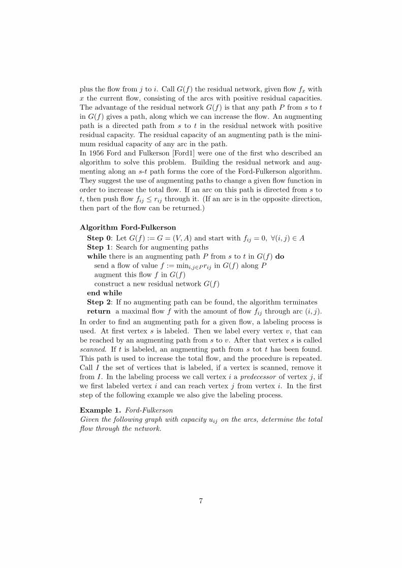
plus the flow from j to i. Call G(f) the residual network, given flow fx withx the current flow, consisting of the arcs with positive residual capacities.The advantage of the residual network G(f) is that any path P from s to tin G(f) gives a path, along which we can increase the flow. An augmentingpath is a directed path from s to t in the residual network with positiveresidual capacity. The residual capacity of an augmenting path is the mini-mum residual capacity of any arc in the path.In 1956 Ford and Fulkerson [Ford1] were one of the first who described analgorithm to solve this problem. Building the residual network and aug-menting along an s-t path forms the core of the Ford-Fulkerson algorithm.They suggest the use of augmenting paths to change a given flow function inorder to increase the total flow. If an arc on this path is directed from s tot, then push flow fij ≤ rij through it. (If an arc is in the opposite direction,then part of the flow can be returned.)
Algorithm Ford-FulkersonStep 0: Let G(f) := G = (V,A) and start with fij = 0, ∀(i, j) ∈ AStep 1: Search for augmenting pathswhile there is an augmenting path P from s to t in G(f) do
send a flow of value f := mini,j∈P rij in G(f) along Paugment this flow f in G(f)construct a new residual network G(f)
end whileStep 2: If no augmenting path can be found, the algorithm terminatesreturn a maximal flow f with the amount of flow fij through arc (i, j).
In order to find an augmenting path for a given flow, a labeling process isused. At first vertex s is labeled. Then we label every vertex v, that canbe reached by an augmenting path from s to v. After that vertex s is calledscanned. If t is labeled, an augmenting path from s tot t has been found.This path is used to increase the total flow, and the procedure is repeated.Call I the set of vertices that is labeled, if a vertex is scanned, remove itfrom I. In the labeling process we call vertex i a predecessor of vertex j, ifwe first labeled vertex i and can reach vertex j from vertex i. In the firststep of the following example we also give the labeling process.
Example 1. Ford-FulkersonGiven the following graph with capacity uij on the arcs, determine the totalflow through the network.
7

ss
s
s
ss
-
-?
6
����
��*
HHHH
HHj
HHHH
HHj
����
��*
15
10
10
10
20
10
20
5
s
1
2
3
4
t
Iteration 11. I = {s}. Vertex s is scanned and vertices 1,2 are labeled, pred(1) =pred(2) = s.2. I = {1, 2}. Vertex 1 is scanned and vertex 3 is labeled, pred(3) = 1.3. I = {2, 3}. Vertex 2 is scanned and vertex 4 is labeled, pred(4) = 2.4. I = {3, 4}. Vertex 3 is scanned and vertex t is labeled, pred(t) = 3.Since vertex t is labeled there is a path from s→ 1→ 3→ t, with mini,j∈P rij =min{15, 10, 20} = 10. This gives the following flow: xs1 = x13 = x3t = 10.We get the following residual graph:
ss
s
s
ss
ji
-?
6-
�HHHH
HHj
I
R
����
��*
5
10
10
10
0
10
20
10
10
10
5
s
1
2
3
4
t
Iteration 2There is a path from s→ 1→ 2→ 4→ t with mini,j∈P rij = min{5, 10, 20, 5} =5. This gives the following flow: xs1 = 15 x12 = x24 = x4t = 5. We get thefollowing residual graph:
ss
s
s
ss
jY
jYN
M 6-
�HHHH
HHj
I
R
�
:
0
15
10
5 5
0
10
15
5
10
10
10
5
0s
1
2
3
4
t
Iteration 3There is a path from s→ 2→ 4→ 3→ t with mini,j∈P rij = min{10, 15, 10, 10} =10. This gives the following flow: xs2 = 10 x24 = 15 x43 = 10 x3t = 15. Weget the following residual graph:
8

ss
s
s
ss
jY
R
I
jYN
M
�-
�
I
R
�
:
0
15
10
05 5
0
10
5
15
0 10
0
20
50
s
1
2
3
4
t
Iteration 4There is no path from s tot t. There is a total flow of 25 through the network,with xs1 = 15, xs2 = 15, x12 = 5, x13 = 10, x24 = 15, x43 = 10, x3t =20, x4t = 5.In the last figure the thick lines give the cut.
We will now state the max-flow min-cut theorem, by Ford and Fulkerson[Ford1]:
Theorem 1. The maximum value of the flow from a source vertex s toa sink vertex t in a capacitated network equals the minimum capacity cutamong all s-t cuts
Proof. If the optimal value of the flow is infinite, it is not hard to see thatthere must exist a directed path P from s to t, such that every arc in P hasinfinite capacity. For every cut S, there is an arc (i, j) belonging to path Psuch that i ∈ S and j /∈ S. Since that arc has infinite capacity, we concludethat u[S, S] = ∞. Since this is true for every cut, we conclude that theminimal cut capacity is infinite and equal to the maximum flow value.Suppose now that the optimal value, denoted by f∗, is finite. (This impliesthat there exists an optimal solution, that is, a flow whose value is f∗.)Let us apply the Ford-Fulkerson algorithm, starting with an optimal flowand the corresponding residual graph. Due to optimality of the initial flow,no flow augmentation is possible, and the algorithm terminates at the firstiteration. Let S be the set of labeled vertices at termination. Since thesearch for an augmenting path starts by labeling s, we have s ∈ S. On theother hand, since no augmenting path was found, t is not labeled i.e. t ∈ Swhere S is the complement of S. Therefore the set (S, S) is a cut. Forevery arc (i, j) ∈ A, with i ∈ S and j /∈ S we must have fij = uij , otherwisevertices j would have been labeled by the labeling algorithm. Thus the totalamount of flow that crosses the set (S, S) is equal to u[S, S], so u[S, S] = f∗.It follows that u[S, S] is the minimum cut capacity and it is equal to thevalue of the maximum flow.
Since this theorem relates the optimal values of a minimization and a max-imization problem, it is a duality theorem. More information can be foundin [Bert].
9

3.2.2 The minimal cost flow problem
The minimal cost flow problem determines a least cost flow through thenetwork that satisfies demands at the vertices from available supplies atvertices. Let G = (V,A) be a directed graph where each arc (i, j) ∈ A has acost cij per unit flow on the arc. Each arc (i, j) also has a capacity uij thatdenotes the maximum amount of flow on the arc. Associated with each ver-tex i ∈ V is an integer number b(i) representing its supply, b(i) > 0, and itsdemand, b(i) < 0. The problem has a feasible solution when
∑ni=1 b(i) = 0.
If the (starting) problem does not satisfies this requirement dummy verticesare introduces.The minimum cost flow problem is an optimization model formulated asfollows:Minimize
∑(i,j)∈A cijxij
subject to∑
j xij −∑
j xji = b(i) for all i ∈ V,0 ≤ xij ≤ uij for all (i, j) ∈ A.For more information about network flows and its variations see the bookNetwork Flows [Ahuj].
3.3 The traveling salesman problem
The problem of finding the shortest path that goes through every vertexof the graph exactly once, and returns to the start, is called the travelingsalesman problem (TSP). The TSP is NP-hard. If the conjecture P 6= NP istrue, then a polynomial-time algorithm for solving the TSP does not exist,which implies that the worst-case running time for any algorithm for TSPincreases exponentially with the number of vertices in the graph. Someinstances with only hundreds of vertices could take many CPU (central pro-cessing unit) years to solve exactly. So, this is another kind of problemcompared to the shortest path problem and maximum flow problem, whichcan be solved in polynomial-time.Since the 1950’s and 1960’s the popularity of the problem has increased,because it plays a central role in logistics and also in algorithm developmentin combinatorial optimization. Danzig, Fulkerson and Johnson introducedin 1954 [Dan2] an integer linear programming formulation and solved theproblem for 49 vertices (cities) with a cutting plane method. In the 1970’sand 1980’s it was possible to solve instances with up to 2392 vertices usingcutting planes and branch and bound. The largest instance solved to opti-mality, has 85900 vertices (cities) and was solved in 2006 [Appl].An often used heuristic to find good feasible solutions to the TSP is thenearest neighbor heuristic (NNH). The running time for this heuristic isO(n2) and if the triangle inequality holds the worst-case solution value isΘ(logn) times the optimal solution, with n being the number of vertices.
10
Christofides [Chri] developed an approximation algorithm that for any in-stance satisfying the triangle inequality produces a feasible solution withvalue less than or equal to 3
2 times the optimal value. This is the best ap-proximation algorithm known for this variant of the TSP. If the lengths ofthe arcs represent Euclidean distances then the best approximation algo-rithm is a (1 + 1
ε )-algorithm with ε > 1 [Aror].In the asymmetric TSP, the distance between two vertices in the underlyingnetwork is not necessary the same in both directions. When the triangle in-equality holds, the best approximation ratio known is obtained by Asadpouret al. and gives a solution within a factor O(log n/log log n) of the optimumwith high probability [Asad]. If no triangle inequality is imposed, there isno polynomial-time algorithm with constant approximation guarantee, forthe asymmetric TSP. For more information about the TSP see [Appl2] orwww.tsp.gatech.edu.
3.4 The vehicle routing problem
When the TSP is expanded with more than one route, it is called the vehiclerouting problem (VRP). The VRP plays a vital role in distribution andlogistics. We all make use of the system around us with routed messages,goods or people from one place to another. In the modern world we needvehicle routing to structure and find the optimal routes. The VRP is theproblem of finding a set of shortest routes with a minimal cost for a fleetof vehicles. The set of vertices (costumers) is divided into subsets, suchthat each subset is serviced by one vehicle. Each vehicle starts and endsat the depot. In the basic problem it is assumed that each vehicle has thesame fixed capacity. The sum of the demands of the visited customers ona route must not exceed the capacity of the vehicle. The problem has beenanalyzed extensively in the literature. Since the problem is NP-hard it isunlikely that a polynomial-time algorithm will be developed for determiningits optimal solution. Consequently a great deal of work has been devoted tothe development of heuristic algorithms.Below we present several variations of the VRP.
• The VRP with time windows (VRPTW). Each customer must be vis-ited within its own given time window. The depot also has its owntime window. The time windows are defined as an interval in whichthe vehicle is allowed to arrive and depart at each customer (vertex).The costumers can have soft or hard time windows. When there arehard time windows there is a strict lower and upper bound. If the ve-hicle arrives before the lower bound, waiting time has to be taken intoaccount. If it arrives too late the problem becomes infeasible. If thereare soft time windows a vehicle can arrive before the lower bound orafter the upper bound. If the vehicle is too early it has to wait, which
11

incurs cost. If it is too late it gets a penalty for lateness.
• There are a lot of different vehicles possible. The vehicle fleet can beheterogeneous, with each vehicle k having a different capacity bk. Itis also possible to have multiple capacity constraints. For example ifthere are both weight and volume restrictions.
• A vehicle may be capable of making more than one trip within aplanning period, or a vehicle may both deliver and pick up products.
• There may be multiple depots with each vehicle assigned to a partic-ular depot. Then the problem can be split into small VRPs with onedepot.
• In the on-line VRP not all the customers are known at the start of theroute. At every costumer, the vehicle has to calculate a new route.
3.4.1 Solution methods for the vehicle routing problem
Huge research efforts have been devoted to studying the VRP since 1959when Dantzig and Ramser [Dant] first described the problem mathemat-ically. Many exact methods have been used to solve the VRP, such asalgorithms based on linear programming techniques. Besides that, to findgood feasible solutions for large-scale VRPs by heuristic techniques havereceived wide interests. The simple heuristics can be grouped into threecategories: route building heuristics, route improvement heuristics, and two-phase methods.Route buildings heuristics select arcs sequentially until a feasible solutionhas been created. For example start with a solution in which every city issupplied individually by a separate vehicle. This is a very expensive solu-tion and if there are not enough vehicles it gives an infeasible solution. Bycombining any two of these routes, we would use one vehicle less and alsoreduce distance. Arcs are chosen based on some distance minimization cri-terion subject to the restriction that the selection does not create a violationof vehicle capacity constraints.A route improvement heuristic begins with a set of arcs S ⊆ A that consti-tutes a feasible schedule and seeks an interchange of a set S1 ⊂ S with a setS2 ⊂ A− S that reduces distance while maintaining feasibility.Two-phase methods first assign cities to vehicles without specifying the se-quence in which they are to be visited. Second, the routes are obtained foreach vehicle using some TSP algorithm. An example is the ’Sweep’ algo-rithm which is only applicable to problems in which cities are located atpoints in the plane and cij is the Euclidean distance. The cities are repre-sented in a system with the origin at the depot. A city is chosen at randomand the ray from the origin through the city is swept either clockwise or
12
counterclockwise. Cities are assigned to a given vehicle as they are swept,until further assignments of cities would exceed the capacity of that vehicle.Another class of heuristics are mathematical programming based heuristics,which are very different in character from the simple heuristics. This line ofresearch began in the mid to late 70’s when a number of researchers beganto apply the machinery of mathematical programming to the VRP. For moreinformation about the VRP see [Ball].Recently, VRP exact algorithms have been based on either branch-and-cutor Lagrangian relaxation/column generation. Fukasawa et al. [Fuka] de-scribed in 2006 an algorithm that combines both approaches, which worksover the intersection of two polytopes. The methode of Fukasawa et al. isequivalent to a linear program with exponentially many variables and con-straints that can lead to lower bounds that are superior to those given byprevious methods. Their branch-and-cut-and-price algorithm can solve, tooptimality, all instances known from the literature with up to 135 vertices.
13
4. Time dependent shortestpaths
Due to the increasing interest in dynamic management of transportationsystems, it is important to find shortest paths where the weights (or delays)associated with arcs dynamically change over time. If real-time traffic infor-mation is available and the standard traffic patterns are known with highprobability, it becomes possible to provide users with better services, suchas “how to travel from one city to another city as fast as possible”, by takingrush hour congestion into consideration.To formulate this problem mathematically we need the definition of a time-dependent graph. A time-dependent graph is defined as GT (V,A,W ) withV a set of vertices, A a set of arcs and W a set of positive valued functions.For every arc (i, j) ∈ A, there is an arc-duration function wij(t) ∈W , wheret is a time variable in a time domain T . The function wij(t) specifies howmuch time it takes to travel from vertex i to vertex j, if departing i at timet. There are different ways to define the arc duration function. It can bedefined to be continuous, or stochastic, or to be the speed of an arc thatdepends on a time interval. From now on we call the source vertex vs andthe sink vertex vd, because we need t to indicate time.
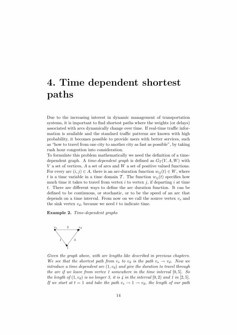
Example 2. Time-dependent graphs
ss
s-SSSSw����7
vs
1
vd3
1 3
Given the graph above, with arc lengths like described in previous chapters.We see that the shortest path from vs to vd is the path vs → vd. Now weintroduce a time dependent arc (1, vd) and give the duration to travel throughthe arc if we leave from vertex 1 somewhere in the time interval [0, 5]. Sothe length of (1, vd) is no longer 3, it is 4 in the interval [0, 2) and 1 in [2, 5].If we start at t = 1 and take the path vs → 1 → vd, the length of our path
14

is 2. This is the fastest way to travel from vertex vs to vertex vd if we taketime into account.
We assume that the time dependent graph satisfies the FIFO-property onthe arcs. The FIFO-property in GT states that if departing earlier fromvertex i one arrives earlier at vertex j, if one travels the same route. So itis not advantageous to delay a departure time. For the time dependent arcsthis mean that every arc (i, j) has the FIFO-property, if∀ t∆ ≥ 0 : wij(ti) ≤ t∆ + wij(ti + t∆)or ti + wij(ti) ≤ tj + wij(tj) for ti ≤ tjWhere ti is the departure time at vertex i and t∆ a small time interval.It is also possible to transform a non-FIFO time dependent graph into atime dependent graph with FIFO-property on the arcs by inserting somewaiting time on each vertex in the optimal shortest path.
Example 3. From non-FIFO to FIFO
ss
ss�
�����*
HHHHHHj?
HHHHHHj
�����
�*vs
1
2
vd
10
2
5
20
Suppose that the durations on arcs (vs, 1), (vs, 2), (1, 2) and (1, vd) are con-stant over time, and are given in the graph above. The duration on arc(2, vd) is equal to 10 in interval [0, 9] and and equal to 5 in interval (9, 20].Assume we start at t = 0. At t = 2 we arrive at vertex 1. We leave vertex1 at t = 2 and arrive at vertex 2 at t = 7. This looks like the fastest pathto follow. When we leave vertex 2 at time t = 7 we arrive at vertex vd att = 17.If we left vertex 2 at t = 10 (so we came from arc (vs, 2)) we would arrivedat vertex vd at t = 15. This means that if we leave vertex 2 later we willarrive earlier on vertex 2. This is a non-FIFO graph.To make the FIFO-property hold, we introduce a waiting time. In this ex-ample you can see that if you travel through vertex 1 (which is the quickestway to go to vertex 2) it is faster path to wait a time period of 3 at vertex 2.
For all the functions w′ij(t) in the non-FIFO graph G
′T we define wij(t) to
construct a FIFO graph GT .wij(t) = ∆ij(t) + w
′ij(t+ ∆ij(t)) = min0≤t∆≤td−t{t∆ + w
′ij(t+ t∆)}
Here tt is the end time, ∆ij(t) is the minimal waiting time required at vertexi to go to vertex j, to make the graph satisfy FIFO and t∆ all the possibletime intervals to wait. Since the starting time interval T is a closed interval,wij(t) and ∆ij(t) are well defined. If there are multiple possible values oft∆ to minimize t∆ + w
′ij(t + t∆), we select any of them as ∆ij(t). It also
satisfies to keep the slope of the arc duration functions between 1 and −1.
15

4.1 A shortest path algorithm for a given startingtime
Given a source vs and a starting time ts, we look for the shortest pathsand minimum delays between vs and all other vertices for that startingtime. In 1969 Dreyfus [Drey] already noted that there exist straightforwardextensions to such algorithms as Dijkstra [Dijk] or Ford [Ford3]. We willgive the algorithm described in Orda and Rom [Orda], which is a so-calledlabeling algorithm. Each vertex is labeled by the earliest possible arrivaltime at that vertex, calculated with the given starting time at the source.The vertices get temporary labels Yk and permanent labels Xk (NULLindicating the vertex is not permanently labeled). A temporal label givesthe length of the shortest path to vertex k, that we found until then. Apermanent label gives the length of the shortest path to get to that vertex.The algorithm also saves the predecessor pred(k) for all permanent labeledvertices k, so the vertices that are visited on the shortest path can be foundeffectively. The input is a time dependent graph with functions wij(t) anda given starting time ts.
Algorithm Time dependent shortest path with a given start timeStep 0: InitializationXs = ts; pred(s) = 0; ∀k 6= s Yk =∞, Xk = NULL, pred(k) = 0; j = s;Step 1:for all k : (j, k) ∈ A for which Xk = NULL do
a:Yk = min{Yk, Xj + wjk(Xj)}b:if Yk changed in Step 1a then
Set pred(k) = jend if
end forStep 2:if all vertices have no null X-value then
Stopelse if l is a vertex for which Xl = NULL and such that Yl ≤ Yk ∀k forwhich Xk = NULL then
Set Xl = Yl, j = l and proceed with Step 1.end if
The main difference between a conventional shortest path algorithm and thealgorithm above is the calculation of wjk(Xj) in step 1a. In this step wetake the path with the shortest length in time. Because the starting timeand the functions wij(t) are given, we can calculate wjk(Xj) for every Xj .Then it is just the length of the arc, and with a proof similar to Dijkstra’s
16
algorithm the correctness is proven. The algorithm terminates after O(|V |2)operations. Each path from vs to any vertex j is a shortest path for startingtime ts whose duration is given by Xj − ts. In the literature we could notfind a correctness proof of this algorithm so we give our own proof, inspiredby the proof of Dijkstra’s algorithm.
Theorem 2. The algorithm terminates after O(|V 2|) operations. After ex-ecution, each path from vs to any vertex j is a shortest path from startingtime ts whose delay is given by Xj − ts.
Proof. Let u be the vertex which gave v its present label Yv; namely, Xu +wuv(tu) = Yv, with wuv(tu) a fixed length (duration) of the path from u tov. After this assignment took place, u did not change its label, since wehave chosen u because it has a permanent label. It is not possible that ifdeparting later from vertex u one arrives earlier at vertex v, if one travelsthe same route, because of the FIFO-property. Next, find the vertex whichgave u its final label Yu with pred(u), and repeating this backward search,we trace a path from vs to v whose length is exactly Yv. The backwardsearch finds, in every step, a vertex that has obtained a permanent label ata previous step, and therefore no vertex on this path can occur more thanonce; it can only terminate in vs, which has been assigned its label in Step0.Let us look at the complexity of the algorithm. Let Y ⊆ V be the set ofvertices with a temporary label. In Step 1a one considers each arc connectedto vertex j exactly once. Thus it uses, at most, O(|A|) time. Since we haveno loops or parallel arcs, |A| ≤ |V | × (|V | − 1) ≤ |V |2. Step 1b is of O(1)and is repeated |V | times. In Step 2 the minimum label of the elements ofY has to be found. At the start of the algorithm Y consists of all vertices,Y = V , and then the cardinality of Y decreases by one each time. This canbe done in |Y | − 1 comparisons and the search is repeated |V | times. Thusthe total time spent in Step 2 is O(|V |2). Thus, the whole algorithm is ofO(|V |2) complexity.
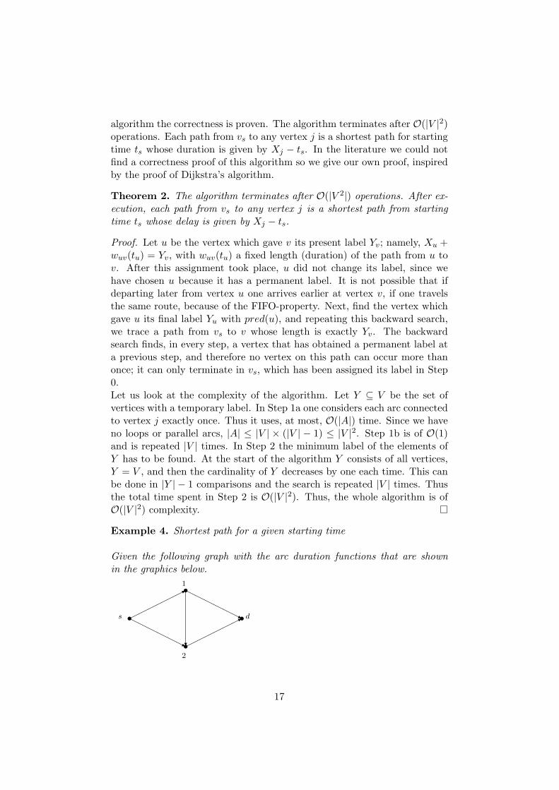
Example 4. Shortest path for a given starting time
Given the following graph with the arc duration functions that are shownin the graphics below.
ss
ss��
����*
HHHH
HHj?
HHHH
HHj
����
��*s
1
2
d
17

0
5
10
5 10 15
ws1(t)
AAAA
0
5
10
5 10 15
ws2(t)
JJJ
0
5
10
5 10 15
w12(t)
@@@
0
5
10
5 10 15
w1d(t)0
5
10
5 10 15
w2d(t)
HHHH
To find the shortest path in time for start time 2 we use the algorithm above.Iteration 1.0. Xs = ts = 2 pred(s) = 0 ∀k 6= s Yk =∞ Xk = NULL pred(k) = 0 j = s1a. k = {1, 2}Y1 = min{∞, Xs + ws1(Xs)} = min{∞, 2 + ws1(2)} = min{∞, 2 + 5} = 7Y2 = min{∞, Xs + ws2(Xs)} = min{∞, 2 + ws2(2)} = min{∞, 2 + 8} = 101b. pred(1) = s pred(2) = s2. l = 1 X1 = 7 j = 1Iteration 2.1a. k = {t, 2}Yd = min{∞, X1 + w1d(X1)} = min{∞, 7 + w1d(7)} = min{∞, 7 + 8} = 15Y2 = min{10, X1 + w12(X1)} = min{10, 7 + w12(7)} = min{10, 7 + 2} = 91b. pred(d) = 1 pred(2) = 12. l = 2 X2 = 9 j = 2Iteration 3.1a. k = {d}Yd = min{15, X2 + w2d(X1)} = min{15, 9 + w2d(9)} = min{15, 9 + 5} = 141b. pred(t) = 22. l = t Xt = 14 j = dSo we found a shortest path s→ 1→ 2→ d of length 14.
4.2 A shortest path algorithm for a given startinginterval
Recently Ding, Xu Yu, and Qin (2009)[Ding] described an algorithm to findtime-dependent shortest paths (TDSP) over large graphs. They studiedhow to answer queries of finding the best departure time that minimizes thetotal travel time from one place to another, over a road network, where thetraffic conditions dynamically change over time. The problem is to find the
18
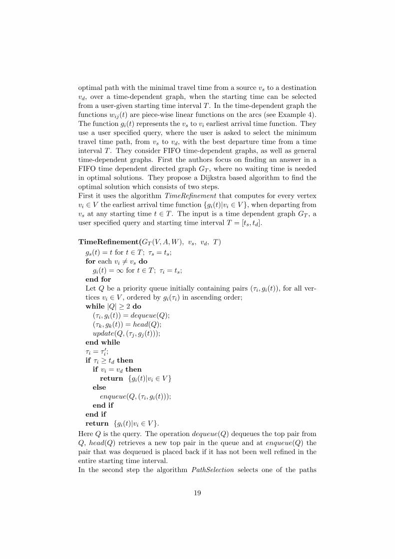
optimal path with the minimal travel time from a source vs to a destinationvd, over a time-dependent graph, when the starting time can be selectedfrom a user-given starting time interval T . In the time-dependent graph thefunctions wij(t) are piece-wise linear functions on the arcs (see Example 4).The function gi(t) represents the vs to vi earliest arrival time function. Theyuse a user specified query, where the user is asked to select the minimumtravel time path, from vs to vd, with the best departure time from a timeinterval T . They consider FIFO time-dependent graphs, as well as generaltime-dependent graphs. First the authors focus on finding an answer in aFIFO time dependent directed graph GT , where no waiting time is neededin optimal solutions. They propose a Dijkstra based algorithm to find theoptimal solution which consists of two steps.First it uses the algorithm TimeRefinement that computes for every vertexvi ∈ V the earliest arrival time function {gi(t)|vi ∈ V }, when departing fromvs at any starting time t ∈ T . The input is a time dependent graph GT , auser specified query and starting time interval T = [ts, td].
TimeRefinement(GT (V,A,W ), vs, vd, T )gs(t) = t for t ∈ T ; τs = ts;for each vi 6= vs dogi(t) =∞ for t ∈ T ; τi = ts;
end forLet Q be a priority queue initially containing pairs (τi, gi(t)), for all ver-tices vi ∈ V , ordered by gi(τi) in ascending order;while |Q| ≥ 2 do
(τi, gi(t)) = dequeue(Q);(τk, gk(t)) = head(Q);update(Q, (τj , gj(t)));
end whileτi = τ ′i ;if τi ≥ td then
if vi = vd thenreturn {gi(t)|vi ∈ V }
elseenqueue(Q, (τi, gi(t)));
end ifend ifreturn {gi(t)|vi ∈ V }.
Here Q is the query. The operation dequeue(Q) dequeues the top pair fromQ, head(Q) retrieves a new top pair in the queue and at enqueue(Q) thepair that was dequeued is placed back if it has not been well refined in theentire starting time interval.In the second step the algorithm PathSelection selects one of the paths
19

from vs to vd that matches the optimal travel time. The input is the time-dependent graph GT , the set of earliest arrival-time functions gi(t), com-puted from TimeRefinement, for all vertices vi ∈ V , source vs, destinationvd and the optimal starting time t∗.
PathSelection(GT (V,A,W ), {gi(t)}, vs, vd, t∗)vj = vd;p∗ = ∅;while vj 6= vs do
for each (vi, vj) ∈ A doif gi(t∗) + wi,j(gi(t∗)) = gj(t∗) thenvj = vi
end ifend forp∗ = (vi, vj)× p∗;
end whilereturn p∗;
For a technical description of the algorithms, an example and the correctnessproofs, see the article by Ding et al. It is shown that the time complexityis O((nlogn + m)α(T )), where α(T ) is the cost required for each functionoperation. This α(T ) is possibly unbounded because it depends on the rel-ative values of arrival time functions. For an unbounded instance see [Dehn].
4.2.1 Time functions with time intervals
Sung et al. [Sung] presented a flow speed model where the flow speed of eacharc depends on the time intervals. To satisfy the FIFO-property the flowspeed of each arc and not the travel time changes as the interval changes.They use a Dijkstra label setting shortest path based algorithm.Consider a network G = (V,A) and let lij be the non-negative length ofthe arc (i, j). Divide the time horizon into the following time intervals;[fk, fk+1), k = 0, 1, 2, . . . ,K − 1. Let vk(ij)
be the non-negative flow speed intime interval [fk, fk+1) on arc (i, j). Define a value ti = minj 6=i{T (ti, (i, j))}where T (ti, (i, j)) is the arrival time at vertex j starting from vertex i attime ti. In the algorithm, the travel time of each arc is calculated accordingto the flow speed at the time of passing the arc. They only insert a functioncalculating the arrival time at the next connecting vertex of the currentvertex in the Dijkstra algorithm.Let pred(i) be the predecessor vertex of i and let A(i) be the set of all arcsconnected to i. The set of vertices which are not scanned is given by U andS is the set of scanned vertices. Then the combined Dijkstra’s label settingalgorithm is described as follows:
20

Algorithm modified DijkstraS := ∅; U := Vti =∞ for each vertex i ∈ Vts = 0 and pred(s) = 0while |S| < n do
let i ∈ U be a vertex for which ti = min{tj : j ∈ U}S := S ∪ {i}U := U − {i}for each(i, j) ∈ A(i) do
if tj > Arrivaltime(ti, (i, j)) thentj := Arrivaltime(ti, (i, j)) and pred(j) := i
end ifend for
end whileLet Arrivaltime(ti, (i, j)) be the arrival time at vertex j starting from vertexi at time ti. The function that calculates the arrival time is the followingfunction:
Arrivaltime(ti, (i, j))Arclength := lijlet k ∈ {0, 1, 2, . . . ,K} be an index for which fk(i,j)
≤ ti < fk+1(i,j)
Arclength := Arclength− vk(i,j)× (fk+1(i,j)
− ti)while Arclength > 0 dok := k + 1Arclength := Arclength− vk(i,j)
× (fk+1(i,j)− fk(i,j)
)end whileArrivaltime(ti, (i, j)) := fk+1(i,j)
+Arclength/vk(i,j)
returnThe computational complexity of the original Dijkstra’s algorithm is O(n2 +m), where n are the number of vertices in the network en m the numberof arcs. For the modified algorithm it gives O(n2 + mK), where K is themaximum number of time intervals scanned in Arrivaltime.
21

5. Time dependent flows
5.1 Network flows over time
Flow variation over time is an important feature in network flow problemsarising in various applications, an example is road traffic control. Trafficflows have two important features that make them difficult, namely conges-tion and time. Congestion captures the fact that travel times increase withthe amount of flow on the roads and time refers to the movement of carsalong a path as a flow over time. These aspects are not captured by theclassic static networks.Network flows over time include a temporal dimension and therefore providea more realistic modeling tool for numerous real world applications. We willconcentrate on flows over time (also called “dynamic flows” in the literature)with finite time horizon and constant capacities and constant transit timesin a continuous or discrete time model. Here the flow requires a certainamount of time to travel through each arc. So not only the amount of flowis taken into account, also the time it takes to travel through the network.
5.2 Ford and Fulkerson
Ford and Fulkerson first introduced the notion of flows over time and con-structed in 1958 [Ford2] an algorithm to find a maximal dynamic flow froma static flow. The problem is to find the maximal amount of flow that can betransported from one vertex to another in a given number T of time periods,and to determine along which arcs the flow is sent in order to achieve thismaximum. In the article by Ford and Fulkerson there is a computationallyefficient algorithm for solving this dynamic linear programming problem pre-sented. They also give an extensive example on how to use their algorithm.We will give the problem definition and their algorithm. Let G = (V,A)be a directed graph with a source vertex vs ∈ V and a sink vertex vd ∈ V .Each arc (i, j) ∈ A has a capacity uij and a transit time tij . If the graphincludes costs, each arc also has a cost coefficient. The total number of timeperiods, is specified by T . Let v(T ) denote the total amount of flow thatleaves the source and enters the sink during the T periods. Let δ+(v) and
22

δ−(v) denote respectively, the set of arcs (i, j) ∈ A leaving vertex v andentering vertex v.A (static) network flow x assigns a non-negative flow value xij to eacharc (i, j) ∈ A. The flow is feasible if it respects the capacity constraints:0 ≤ xij ≤ uij . An s-d flow x satisfies flow conservation at each vertexv ∈ V \{vs, vd}, that is,
∑(i,j)∈δ−(v) xij −
∑(i,j)∈δ+(v) xij = 0.
5.2.1 The algorithm from Ford and Fulkerson
The algorithm from Ford and Fulkerson [Ford2] constructs a static flow andis essentially a primal dual method for a capacitated transshipment problem.The algorithm is an iterative process that has as final output an integralstatic flow xij , together with a set of integers π(i) for each vertex i in V .π(i) is the so-called vertex potential and gives the travel time, with respectto transit times of arcs, from vs to vertex i. After augmenting flow along theshortest s-d path P k in Gxk , πk(i) is still feasible and k gives the iterationnumber. Here Gxk is the residual network with flow xk. This implies thatthe shortest path distances have not been decreased. All the π(i) have tosatisfy the following constraints:
π(s) = 0, π(t) = T + 1, π(i) ≥ 0 (5.1)
π(i) + tij > π(j) for xij = 0 (5.2)
π(i) + tij < π(j) for xij = uij (5.3)
To start the algorithm take all xij = 0 and all π(i) = 0.Arcs (i, j) for which π(i) + tij = π(j) will be called admissible arcs. Notethat at most one member of the pair (i, j), (j, i) will be admissible. Duringthe algorithm a vertex is either unlabeled, or labeled but unscanned, orlabeled and scanned. If a vertex gets a label like [v±k , h], the label says thatvertex vk is the predecessor of this vertex and it is possible to send a flowwith value h to this vertex. The position of the ± gives the direction of theflow, a + if it is directed from vs to vd and − if the flow is directed in theopposite direction. A vertex is scanned if all the labels of its neighbors areupdated. Start with all vertices unlabeled.
Algorithm Ford and Fulkerson with time
Step 1: Give vs the label [v+d ,∞], and consider vs as unscanned.
Step 2: Select any labeled, unscanned vertex vi, suppose it is labeled [v±k , h].
a: To all vertices vj that are unlabeled and such that (i, j) is admissibleand xij < uij assign the label [v+
i ,min(h, uij − xij)]. All vj arenow labeled and unscanned.
23

b: To all vertices vj that are now unlabeled and such that (j, i) isadmissible and xji > 0 assign the label [v−i ,min(h, xji)]. Such vjare now labeled and unscanned.
c: Now define vi to be labeled and scanned.
Repeat this step until the sink vd is labeled and unscanned, or untilno more labels can be assigned. In the former case go to Step 3. Inthe latter case, let the present flow be denoted by the new name x
′ij ,
and go to Step 4.
Step 3: Update the flow.
a: If vd is labeled [v+k , h] replace xkd by xkd + h.
b: If vd is labeled [v−k , h] replace xkd by xkd − h.
c: Go to vertex vk and treat it the same way as vertex vd.
Repeat until vs is reached. Now the replacement process is stopped.This process alters the flow along a path from vd to vs.Discard all labels and return to Step 2 with the new flow.
Step 4: Define π′(i) by
π′(i) =
{π(i) if vi is labeled;π(i) + 1 if vi is unlabeled.
Repeat the algorithm, starting with x′ij and π
′(i) and continuing until
the value of π(t) has been increased to T + 1.
Example 5. Ford and Fulkerson with timeGiven the following graph with capacity uij and time tij on the arcs, deter-mine the total flow through the network.
ss
ss
s
ss
-
HHHH
HHj-
?
?
6
����
��*
-HHHH
HHj
HHHH
HHj
����
��*
2,20
1,20
3,20
3,10
3,10
2,20
3,20
2,10
5,10
2,10
3,30
vs
1
2
3
4
5
vd
Take for the time period T = [0, 8] and start with π(i) = 0.Iteration 1a Label vs : [v+
d ,∞]b There are no admissible arcs. vd has no label.d π(vs) = 0, π(i) = 1 for i 6= vs
Iteration 2
24

a Label vs : [v+d ,∞]
b Label v2 : [v+s , 20]. vd has no label.
d π(vs) = 0, π(2) = 1, π(i) = 2 for i 6= vs, 2
Iteration 3a Label vs : [v+
d ,∞]b Label v1 : [v+
s , 20]. vd has no label.d π(vs) = 0, π(2) = 1, π(1) = 2, π(i) = 3 for i 6= vs, 1, 2
Iteration 4a Label vs : [v+
d ,∞]b Label v3 : [v+
s , 20]. vd has no label.d π(vs) = 0, π(2) = 1, π(1) = 2, π(3) = 3, π(i) = 4 for i 6= vs, 1, 2, 3
Iteration 5a Label vs : [v+
d ,∞]b Label v4 : [v+
1 , 20] and v5 : [v+2 , 20]. vd has no label.
d π(vs) = 0, π(2) = 1, π(1) = 2, π(3) = 3, π(4) = π(5) = 4, π(vd) = 5
Iteration 6a Label vs : [v+
d ,∞]b No new labels can be added. vd has no label.d π(vs) = 0, π(2) = 1, π(1) = 2, π(3) = 3, π(4) = π(5) = 4, π(vd) = 6
Iteration 7a Label vs : [v+
d ,∞]b Label vd : [v+
4 , 10]. vd has a labelc There is a path from vertex vs to vd. This gives x4d = x14 = xs1 = 10.The arc (4, vd) is the cut. We delete all the labels.a Label vs : [v+
d ,∞]b Label v2 : [v+
s , 20], v1 : [v+s , 10], v3 : [v+
s , 20], v4 : [v+1 , 10] and v5 : [v+
2 , 20].vd has no label.d π(vs) = 0, π(2) = 1, π(1) = 2, π(3) = 3, π(4) = π(5) = 4, π(vd) = 7
Iteration 8a Label vs : [v+
d ,∞]b Label vd : [v+
5 , 20]. vd has a labelc There is a path from vertex vs to vd. This gives x5d = x25 = xs2 = 20.There are no arcs used from the first path so we can send another flowthrough that path which starts 1 time period later. The arcs (4, vd), (vs, 2)and (2, 5) form a cut. We delete all the labels.a Label vs : [v+
d ,∞]b Label v1 : [v+
s , 10], v3 : [v+s , 20] and v4 : [v+
1 , 10]. vd has no label.d π(vs) = 0, π(2) = 2, π(1) = 2, π(3) = 3, π(4) = 4, π(5) = 5, π(vd) = 8
25
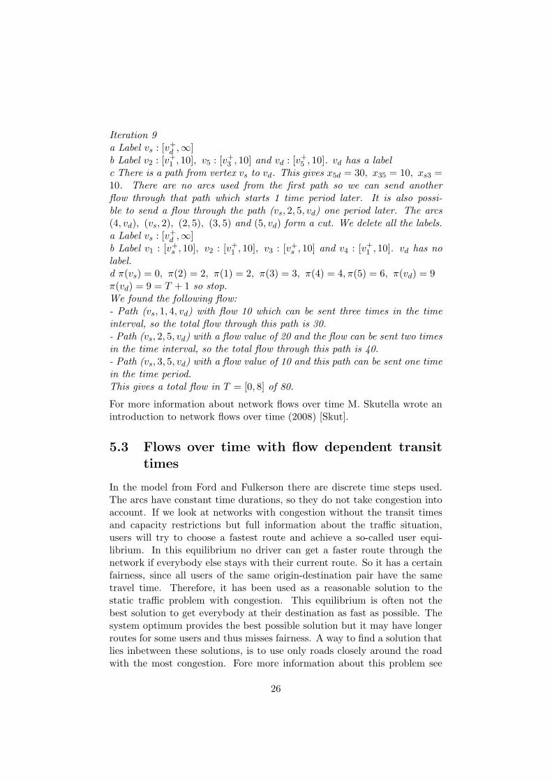
Iteration 9a Label vs : [v+
d ,∞]b Label v2 : [v+
1 , 10], v5 : [v+3 , 10] and vd : [v+
5 , 10]. vd has a labelc There is a path from vertex vs to vd. This gives x5d = 30, x35 = 10, xs3 =10. There are no arcs used from the first path so we can send anotherflow through that path which starts 1 time period later. It is also possi-ble to send a flow through the path (vs, 2, 5, vd) one period later. The arcs(4, vd), (vs, 2), (2, 5), (3, 5) and (5, vd) form a cut. We delete all the labels.a Label vs : [v+
d ,∞]b Label v1 : [v+
s , 10], v2 : [v+1 , 10], v3 : [v+
s , 10] and v4 : [v+1 , 10]. vd has no
label.d π(vs) = 0, π(2) = 2, π(1) = 2, π(3) = 3, π(4) = 4, π(5) = 6, π(vd) = 9π(vd) = 9 = T + 1 so stop.We found the following flow:- Path (vs, 1, 4, vd) with flow 10 which can be sent three times in the timeinterval, so the total flow through this path is 30.- Path (vs, 2, 5, vd) with a flow value of 20 and the flow can be sent two timesin the time interval, so the total flow through this path is 40.- Path (vs, 3, 5, vd) with a flow value of 10 and this path can be sent one timein the time period.This gives a total flow in T = [0, 8] of 80.
For more information about network flows over time M. Skutella wrote anintroduction to network flows over time (2008) [Skut].
5.3 Flows over time with flow dependent transittimes
In the model from Ford and Fulkerson there are discrete time steps used.The arcs have constant time durations, so they do not take congestion intoaccount. If we look at networks with congestion without the transit timesand capacity restrictions but full information about the traffic situation,users will try to choose a fastest route and achieve a so-called user equi-librium. In this equilibrium no driver can get a faster route through thenetwork if everybody else stays with their current route. So it has a certainfairness, since all users of the same origin-destination pair have the sametravel time. Therefore, it has been used as a reasonable solution to thestatic traffic problem with congestion. This equilibrium is often not thebest solution to get everybody at their destination as fast as possible. Thesystem optimum provides the best possible solution but it may have longerroutes for some users and thus misses fairness. A way to find a solution thatlies inbetween these solutions, is to use only roads closely around the roadwith the most congestion. Fore more information about this problem see
26

Kohler, Mohring and Skutella’s article about traffic networks and flows overtime [Kohl].Now we will look at networks where the duration of an arc changes overtime. The field of flows over time with flow dependent transit times has at-tracted attention only in the last couple of years. One reason for this seemsto be the lack of well defined models for this kind of flows, which is due tothe more complicated setting. There are hardly any algorithmic techniquesknown which are capable of providing reasonable solutions even for networksof small size.One problem is how to define the transit time functions. Often they relyon relatively simple functions which are simplifications of the actual flow.Another problem is the definition of the transit time and flow on a particulararc. Do we take the flow at the beginning of the arc, at the moment that theflow enters the arc or is the total amount of flow that is on the arc consid-ered? With congestion these two values could be different. Again, we takethe FIFO-property into account, overtaking of flow units is not permitted.A model that shows that there is at least a good temporally repeated flowfor this problem was suggested by Kohler and Skutella [Koh2]. It is inspiredby the earlier mentioned result of Ford an Fulkerson.Another way to model this problem is based on the time-expanded network.This network contains one copy of the subgraph based on the vertices thatcan be reached in each discrete time step. So there are time layers created.A discrete time flow over time in the given network can be interpreted asa static flow in the corresponding time expanded network. One can applythe algorithms developed for static networks flows to this generalized time-expanded network. The underlying assumption for this approach is that atany moment of time the transit time on an arc only depends on the cur-rent rate of inflow into that arc. However, when considering large networksthis model is not applicable because the time-expanded network will growenormously.
27

6. Time dependent travelingsalesman problem
The time dependent traveling salesman problem (TDTSP) is a generaliza-tion of the TSP where the travel time (cost) between two cities depends onthe moment of the day the arc is traveled.According to Picard and Queyranne (1978) [Pica] the TDTSP was intro-duced by Fox (1973), where it was illustrated with examples from the brew-ing industry. Several linear integer programming formulations were pre-sented in that work but none was found to lead to a tractable solutionscheme. The paper of Picard and Queyranne (1978) can be considered asone of the basic works about the TDTSP. It presents the first practicallyeffective method for solving TDTSPs with up to 20 vertices. This method isbased on shortest path computations, dynamic programming and a branchand bound algorithm. The travel time between two vertices depends on theposition of the vertices in the sequence of the tour. Their model is still oneof the few exact models proposed in the literature.Malandraki and Daskin (1992) [Mala] described the problem as a specialcase of the TDVRP, where they treated the time function as a step func-tion. In the next chapter we describe their approach. In 1996 Malandrakiand Dial [Mal2] proposed a restricted dynamic programming heuristic (ageneralization of the NNH). The heuristic lets the user choose some middleground between the optimal dynamic programming algorithm and the NNH.This means that only a user-specified number of partial tours is allowed ateach stage. Their heuristic gives a good solution for problems of more than200 vertices. Vander Wiel and Sahinidis [Vand] developed a branch andcut algorithm and applied a Benders decomposition to the problem in orderto speed up lower bound calculation and solved the TDTSP. They solvedinstances having up to 18 nodes to optimality, by embedding their bound ina branch-and-bound algorithm.In 2008 Bigras et al. [Bigr] also presented an exact solution method for theTDTSP. They show how integer programming formulations of the TDTSPcan be extended to single machine scheduling problems with sequence de-pendent setup times. Several integer programming formulations of varying
28

size and strength are introduced. There is an exact branch and bound algo-rithm proposed that is able to solve instances up to 45 vertices.A more recent research by Miranda-Bront et al. (2010) [Mira] considers themodels presented in Picard and Queyranne and Vander Wiel and Sahinidis.Both polytopes are analyzed and families of valid inequalities for both mod-els are derived. They present computational results for a branch and cutalgorithm that uses these inequalities. The results show that their algorithmseems very efficient compared to known algorithms.
6.1 A heuristic algorithm for TDTSP
Many companies deliver products daily and/or weekly to their costumers.To visit all their customers in an optimal way taking rush hours into account,we advice to use the branch and bound algorithm from Bigras et al. If thereare about 25 customers or more it would be faster to use a heuristic, butthen no guarantee of optimality can be given. We give a nearest neighborheuristic that could be used for a problem with time-dependent travel times.Given is a time-dependent graph GT = (V,A,W ), with V = {s, 1, 2 . . . , n}the set of vertices (customers), where vs = s, n are the depot. The set ofpiece-wise continuous functions in W are arc duration functions wij(t) oneach arc (i, j) ∈ A. The vertices have to be visited within a given timehorizon T and ts is the starting time for the tour.In the heuristic we present below, the last vertex of the (sub)route is definedby l, Q is the set of unvisited vertices and R is an ordered set and gives the(sub)route.
NNH algorithm for the TDTSPStep 0:Start at the depot and take l = vs at time ts with Q = {1, 2, . . . , n − 1}and R = {vs}.Step 1:while Q 6= ∅ do
Compute the arrival time at every possible neighbor of l in Q and finda vertex j with the shortest travel time.Mark l as visited and take l = j, Q := Q− j and R := R∪ {j}.
end whileStep 2:If Q = ∅, take the route R which gives a path through all the vertices andadd the travel time from the last vertex to the depot.
In Step 1 it is possible to compute all travel times because the starting timefor the tour is known. We know the exact time we leave from the vertex land the function wij(t) gives the time we arrive at vertex j. The complexityof the NNH is O(n2).
29

One disadvantage of this heuristic is that the travel time between the lastcustomer and the depot could be very long. For the TSP the tour can beimproved by an iterative process. Often 2-opt or k-opt are used, this meansthat in each step two or k arcs will be removed. The fragments will bereconnected by two or k new arcs, such that a new (and shorter) tour iscreated. If we apply this iterative process on the TDTSP it is possible thatmore arcs have to be changed because the arrival times will have changed.Consider an example in which we remove arc (k, l) and arc (p, q). Supposethat (k, l) is the first arc in the tour and that it would give a shorter tour ifwe submit arc (k, p). Then we have to calculate all the other arcs in the tourbecause the arrival times at vertices p, l, q, r have changed. See the figurebelow:
s s s
ss
s@
@@I
���
���3
@@RBBBBN��
���
k
p
l
vs
q
rs s s
ss
s@@
@I
���
�����
-BBBBN��
���
k
p
l
vs
q
r
F igure 1
This shows that if an iterative process is applied after the NNH for theTDTSP, all the arcs have to be recalculated for the new tour. With thesefindings we see that it has no influence how many arcs are removed, so 2-optcould be a good process to use. Another way to improve the tour from theNNH is choosing in each step a different vertex after visiting the depot. Weapply this method n − 1 times, for all the vertices except the depot, andchoose the tour with the shortest travel time. In this case we know that thevery long last arc will be chosen in one tour first and might be shorter.This method gives the following heuristic algorithm for the TDTSP withorder O(n3)
Iterative NNH algorithm for the TDTSPStep 0:Start at the depot l = vs at time ts with Q = {1, 2, . . . , n− 1}, k = 1 andR = {vs}.Step 1:First choose the arc (vs, k). tk is the new starting time, mark vs as visitedand take l = k, Q := Q− k and R := R∪ {k}Step 2:while Q 6= ∅ do
Compute the arrival time at every possible neighbor of l in Q and finda vertex j with the shortest travel time.Mark l as visited and take l = j, Q := Q− j and R := R∪ {j}.
end while
30
Step 3:If Q = ∅, take the route R which gives a path through all the vertices andadd the travel time from the last vertex to the depot to get tour Rk withtime T − ts.Step 4:Take k = k + 1 and repeat Step 1-4 until k = n− 1, then go to Step 5.Step 5:Return the tour with minimal time T − ts.
6.1.1 Quality of the heuristic
A heuristic gives hopefully a good feasible solution for a problem, but theygive in general not the optimal solution. That is why one would like to knowa priori how good the solution of a heuristic is. The quality of a heuristicH, given by q(H), is defined by the worst-case solution of the heuristic.Let H(I) be the worst-case solution of the heuristic, for instance I and letO(I) be the optimal solution of the instance. In the case of a minimizationproblem we have that H(I) ≥ O(I). The quality of heuristic H is definedas q(H) = supP
H(I)O(I) .
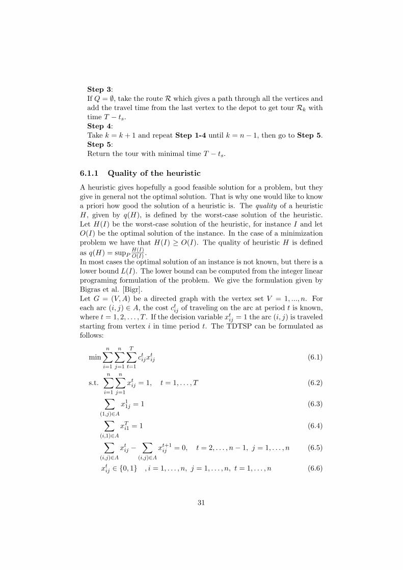
In most cases the optimal solution of an instance is not known, but there is alower bound L(I). The lower bound can be computed from the integer linearprograming formulation of the problem. We give the formulation given byBigras et al. [Bigr].Let G = (V,A) be a directed graph with the vertex set V = 1, ..., n. Foreach arc (i, j) ∈ A, the cost ctij of traveling on the arc at period t is known,where t = 1, 2, . . . , T . If the decision variable xtij = 1 the arc (i, j) is traveledstarting from vertex i in time period t. The TDTSP can be formulated asfollows:
minn∑i=1
n∑j=1
T∑t=1
ctijxtij (6.1)
s.t.n∑i=1
n∑j=1
xtij = 1, t = 1, . . . , T (6.2)
∑(1,j)∈A
x11j = 1 (6.3)
∑(i,1)∈A
xTi1 = 1 (6.4)
∑(i,j)∈A
xtij −∑
(i,j)∈A
xt+1ij = 0, t = 2, . . . , n− 1, j = 1, . . . , n (6.5)
xtij ∈ {0, 1} , i = 1, . . . , n, j = 1, . . . , n, t = 1, . . . , n (6.6)
31
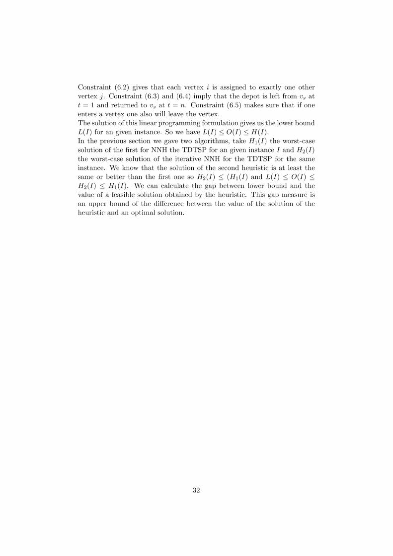
Constraint (6.2) gives that each vertex i is assigned to exactly one othervertex j. Constraint (6.3) and (6.4) imply that the depot is left from vs att = 1 and returned to vs at t = n. Constraint (6.5) makes sure that if oneenters a vertex one also will leave the vertex.The solution of this linear programming formulation gives us the lower boundL(I) for an given instance. So we have L(I) ≤ O(I) ≤ H(I).In the previous section we gave two algorithms, take H1(I) the worst-casesolution of the first for NNH the TDTSP for an given instance I and H2(I)the worst-case solution of the iterative NNH for the TDTSP for the sameinstance. We know that the solution of the second heuristic is at least thesame or better than the first one so H2(I) ≤ (H1(I) and L(I) ≤ O(I) ≤H2(I) ≤ H1(I). We can calculate the gap between lower bound and thevalue of a feasible solution obtained by the heuristic. This gap measure isan upper bound of the difference between the value of the solution of theheuristic and an optimal solution.
32
7. Time dependent vehiclerouting problem
Most of the models for the VRP that are described in the literature, likewe noted in chapter 3.4, assume constant travel times. Clearly, ignoringthe fact that the travel time between two customers does not depend onlyon the distance traveled, but also on the time of the day, has impact onthe application of these models to real-world problems. The time dependentvehicle routing problem (TDVRP) has the same variants as the VRP buthere the travel times depend on the time of day. The TDVRP has seldombeen studied because they are harder to model and more difficult to solvethan the VRP. We give a comprehensive overview about the literature wefound on TDVRPs.
7.1 Literature
Malandraki and Daskin (1992) [Mala] were the first to formulate the TD-VRP. They used a mixed integer linear programming formulation. In theformulation of the problem an n × n time dependent matrix C(t) = cij(ti)was used, which gives the travel times on an arc (i, j) ∈ A as a function ofthe time t. In this matrix, cij(ti) is a step function of the time of the daywith ti at vertex i. Each arc (i, j) is replaced by Mij parallel arcs, whereMij) is the number of distinct time intervals considered in the step functioncij(ti). The depot is expanded by K vertices (n+ 1, . . . , n+K) correspond-ing to returning depot vertices for each of the K vehicles. The aim is tominimize the total routing time (travel time plus service time plus waitingtime). The following constraints are used:K = number of vehiclesn = number of vertices including the depotM = number of time intervals considered for each arccmij = travel time from vertex i to j if starting at i during time interval m;cmii =∞ ∀i,mci = service time at vertex im; ci = 0 at the depotTmij = upper bound for time interval m for arc (i, j)
33

t = the starting time from the depotsbk = weight capacity of vehicle kdi = weight to be collected at customer iB1, B2 = a large numberB = maxkbk = capacity of large vehicleLi = earliest time that the salesman can arrive at vertex iUi = latest time that the salesman can arrive at vertex itj = departure time of any vehicle from vertex jwj ≥ weight that carried by a vehicle when departing from vertex jxmij is a decision variable and is 1 if any vehicle travels directly from vertexi to vertex j starting from i during time interval m ans is 0 otherwise.The TDVRP may be formulated as follows:
minK∑k=1
tn+k (7.1)
s.t.n∑i=1
M∑m=1
xmij = 1, j = 2, . . . , n+K (7.2)
n+K∑j=2
M∑m=1
xmij = 1 , i = 2, . . . , n, (7.3)
n∑j=2
M∑m=1
xmij = K (7.4)
t1 = t (7.5)tj − ti −B1x
mij ≥ cmij + cj −B1 (7.6)
ti +B2xmij ≤ Tmij +B2 (7.7)
ti − Tm−1ij xmij ≥ 0 (7.8)
for 7.6, 7.7, 7.8 (i = 1, . . . , n; j = 2, . . . , n+K; i 6= j; m = 1, . . . ,M)Li + ci ≤ ti ≤ Ui + ci , i = 1, . . . , n+K (7.9)
wj − wi −BM∑m=1
xmij ≥ dj −B (i = 1, . . . , n; j = 2, . . . , n+K; i 6= j)
(7.10)
w1 = 0 (7.11)wn+k ≤ bk (k = 1, . . . ,K) (7.12)xmij ∈ {0, 1} ∀i, j,m (7.13)
ti ≥ 0, wi ≥ 0 ∀i (7.14)
In the formulation of the problem, waiting at a vertex is allowed. Con-straints (7.2) to (7.4) ensure that each customer is visited exactly once and
34
that exactly K vehicles are used. Constraints (7.6) compute the departuretime at vertex j. The objective function (7.1) ensures that this constraintis applied with equality when xmij = 1 except in cases where waiting at jdecreases the objective function value. The temporal constraints (7.7) and(7.8) ensure that the proper parallel arc m is chosen between vertices i andj according to the departure time from i. We want to model the followingconstraints: if xmij = 1 then Tm−1
ij ≤ ti ≤ Tmij ∀i, j,m. This means that tibelongs to the time interval m defined by the above inequalities if the arcused corresponds to the same time interval m. We can set the large numberB2 equal to the latest possible return time of a vehicle. Constraints (7.9)impose the time windows that are defined in terms of the arrival times atthe vertices. Constraints (7.10) to (7.12) impose the capacity restrictions.Constraint (7.11) states that all vehicles leave the depot empty. Constraint(7.10) ensure that the weight carried by the vehicle leaving customer j isat least equal to the weight when leaving the previously visited customer iplus the weight of the commodity picked up. Constraint (7.12) ensure thatthe capacity of each vehicle is not exceeded.The problem does not take the FIFO-property into account. In the article,heuristics are given for the TDTSP and TDVRP without time windows. Thealgorithms are based on the nearest neighbor (greedy) heuristic (NNH) forthe traveling salesman problem. For the TDVRP a heuristic sequential routeconstruction is given. A new vehicle is only introduced when no customercan be assigned using the current vehicle(s). In this case the worst runtimeperformance is bounded by O(n2M). Another heuristic, simultaneous routeconstruction, is given. In this heuristic, a new vehicle is introduced, at anystate of the algorithm, when this leads to the use of the shortest arc thatdoes not violate the temporal requirements and the capacity of the vehicle.A solution can be obtained in O(n2KM) time, with K being the numberof vehicles. When the total capacity is much larger than the total demand,then one should avoid using this algorithm. In addition, a cutting planeheuristic algorithm for the TDTSP with a given starting time from the de-pot, and without time windows, is briefly discussed. The algorithms aretested on randomly generated problems with 10 to 25 vertices. The traveltimes are represented by step functions of two or three time periods perarc on average. The NNH requires very low computing times. The cuttingplane algorithm is much more computationally expensive and solves onlysmall problems but finds a solution better than, or at least as good as thesolution obtained by the NNH in two of the three problems tested.In 2003 Ichoua, Gendreau and Potvin [Icho] proposed a tabu search solu-tion method in order to heuristically solve TDVRPs with soft time windowsand which guarantees the FIFO-property. Like Malandraki and Daskin, thismodel uses a time-dependent matrix C(t), with p different time periods. Thespeed of the vehicle changes when the boundary between two consecutivetime periods is crossed. Because the travel speed is a step function, the
35
travel time is a piece-wise continuous function over time. The objective isto minimize a weighted sum of total distance traveled and total lateness overall customers. The algorithm uses parallel tabu search developed by Taillard(1997). The method is tested using Solomon’s 100 customer problems. Inthese problems customer locations are generated randomly and uniformlywithin a [0, 100]2 square. The experiments were performed to evaluate themodel in a static and dynamic environment. Three time periods and threetypes of time dependent arcs are studied. The results of their experimentsshow that the time-dependent model provides very significant improvementsto the objective value over the model with fixed travel times, thus indicatingthe usefulness of additional information about the problem.Fleischmann, Gietz and Gnutzmann (2004) [Flei] use traffic information ofBerlin to see whether they could improve vehicle routing and scheduling.They present a general framework for the implementation of time-varyingtravel times in various vehicle routing algorithms that were already proposedin the literature. The goal was to minimize the number of vehicles and totaltravel time. Computational tests based on the traffic in Berlin shows thatthe use of constant average travel times can lead to significant underestima-tion of the actual total travel times.More recently, Van Woensel, Kerbache, Peremans, and Vandaele (2008)[Woen] used a tabu search algorithm to heuristically solve the TDVRP.They used approximations based on queuing theory to determine the travelspeeds. The objective is to find the minimum cost vehicle routes. Threedifferent speed approaches are compared: no speed effects, three time pe-riods (morning, mid-day and evening) and a queuing model with 144 timeintervals. A dataset with real-life observations is used as input. For eachof the three speed approaches there are solutions generated using the tabusearch heuristic. These solutions are re-evaluated using a different valida-tion dataset for a different comparable day. The results show that the totaltravel time can be improved significantly, when explicitly taking congestioninto account during the optimization. Additionally the authors found that ahigher number of time zones improves the solution quality. Another findingis that adapting a starting time for a solution has significant effects on theobtained solution quality. The extra computing time for large data sets issignificant but is worthwhile because the solution quality is improved.Soler, Albiach and Martınez (2008) [Sole] use a different approach becausethey transform the TDVRP with time windows through several steps into anasymmetric capacitated VRP, a well-known routing problem. This problemcan be solved optimally and heuristically with known codes. The aim is tominimize the sum of the costs of the different routes given that the travers-ing arc times satisfy the FIFO-property. They provide a way to optimallysolve the problem, at least for small size instances (due to its complexity).An alternative way is described by Donati et al. (2008) [Dona]. The al-gorithm that is used, is based on the ant colony system and local search
36
procedures. The algorithm is named MACS-VRPTW. They describe a TD-VRP with delivery time windows. The basic idea of ant colony optimizationis to use a positive feedback mechanism to reinforce those parts that belongto a good solution, while discarding those that belong to poor solutions.This is done with the possibility to temporally store this information sothat it will be locally available to all the individuals. They combine two al-gorithms, one to optimize the number of vehicles and one for optimizing thetotal travel time. The algorithms are supported by local search proceduresthat store and update the slack times or feasible delays. The algorithmsare tested using some variations of the Solomon problems and on a real-lifenetwork in Padua, Italy.Last year Figliozzi (2009) [Figl] presented a new solution approach, an it-erative route construction and improvement algorithm (IRCI), for the TD-VRP with hard and soft time windows. The improvements are obtained ata route level and do not rely on any type of local improvement procedure.The solution algorithms can handle constant speed at time-dependent speedproblems. A new formulation for the TDVRP with soft and hard time win-dows is presented. The travel speed in any arc is a positive and continuousfunction of time, which guarantees the FIFO-property. The travel timesmay be asymmetric and waiting time at a customer is allowed. The pri-mary objective function is the minimization of the number of routes; theoptimal number of routes is unknown. A secondary objective is the min-imization of the total time or distance. The solution method to minimizefleet size is divided into two phases and heuristics: route construction androute improvement. For the construction heuristic a route building heuristicis presented which will be repeatedly executed. The route building heuristicis a generalized nearest neighbor heuristic. Similarly the route constructionheuristic is repeatedly executed during the improvement heuristic. For anygiven route a dynamic programming approach can be used to determine theoptimal service start times for customers. The performance of the IRCIwas tested on the Solomon instances with constant travel speed and on atime dependent variant. The IRCI is faster than the methods presentedby Donati et al. (2008) but in terms of solution quality the solutions areabout 4% less than the best results ever obtained by the Solomon instances.For the time dependent cases the author did not find similar results, so acomparison was not possible.
7.2 A heuristic for the TDVRP
In 2008 Soler et al. described an idea to solve the TDVRP optimally, bytransforming it into an asymmetric capacitated VRP. The consequences oftheir approach is that the asymmetric capacitated VRP is still a hard prob-lem to solve. These transformations will make the problem size blow up. It
37

would only be possible to do this for small instances. The article is overalltheoretical, and to the best of our knowledge, no computational experimentsusing this approach have been reported so far. To find an optimal solutionfor the TDVRP is not yet a realistic option for real-world instances.We give an approach for a heuristic based on the heuristic for the TDTSPwe presented in Chapter 6.1. The TDVRP can be seen as the problem ofsolving the TDTSP for each vehicle, if the customers are divided throughout the vehicles. In Chapter 3.4.1 we have seen that the customers can bedivided with a sweep method, which seems to be a good idea. The problemin the time dependent case is that some vehicles could have routes involv-ing heavy congestion. It is thus very important to divide the customers ina “good” way over the vehicles. We try to divide the customers in threegroups, the customers with less rush hour traffic in the morning or mid-dayor evening. If there is a congestion in one way from customer i to j, weadvice to place customer i in a later time period than customer j, so thecongestion can be avoided. When the selection is made the algorithm inchapter 6.1 can be applied to each separate vehicle.
38

8. Conclusion
In this master thesis we have studied optimization problems in networkswith time dependent arcs. The aim is to describe real world problems in amore realistic way than the optimization problems with constant arcs.First we looked at the time dependent shortest path problem. We gave analgorithm for this problem where the starting time is known and holds theFIFO-property. The algorithm is based on the Dijkstra algorithm for theshortest path problem. We gave a proof of the algorithm because it couldnot be found in the literature. If the starting point of the time dependentshortest path has to lie in a given starting time interval, there are two ap-proaches given to handle this question. For both methods the complexity ofthe algorithm could be unbounded because it depends on the arrival timefunctions or the number of time intervals which can be exponential.Secondly, time dependent flows are examined. The first algorithm ever tofind a maximal flow over time, by Ford and Fulkerson, is given. To also takecongestion into account, a time-expanded network that contains time layersis explained. On this network an algorithm for a static flow can be applied.The time-expanded network grows with the number of time intervals so itcould get very large.Another problem we studied is the time dependent extension of the trav-eling salesman problem. We gave a nearest neighbor heuristic to achieve atour for a given starting time. The NNH could give a much different tourfrom the optimal solution, that is why we improve the tour by iterativelyapplying the NNH. There will be n − 1 tours calculated and the shortesttour in time is chosen.Finally, the time dependent vehicle routing problem is discussed by giving acomprehensive literature overview and suggestions for solving the problem.There is almost no information known to derive an optimal solution. Lastyear Figliozzi described a heuristic for this problem and gave some results.To evaluate this heuristic theoretically and computationally seems an in-teresting avenue for future research. We like to recommend this for futureresearch. Furthermore, it would be interesting to look at the time windowsof the TDVRP and to study the problems from this thesis for a given start-ing time interval and see if it is possible to formulate polynomial heuristicsthat could produce good-quality solutions for realistic instances.
39

Appendix A
FIFO: First In First OutNNH: Nearest Neighbor Heuristic TDSP: Time Dependent Shortest PathTDTSP: Time Dependent Traveling Salesman ProblemTDVRP: Time Dependent Vehicle Routing ProblemTSP: Traveling Salesman ProblemVRP: Vehicle Routing ProblemVRPTW: Vehicle Routing Problem with Time WindowsIRCI: Iterative Route Construction and Improvement algorithm
40

Bibliography
[Ahuj] Ahuja, R.K., Magnanti, T.L., Orlin, J.B. Network Flows: Theory,Algorithms, and Applications. Prentice Hall (1993)
[Appl] Applegate, D.L., Bixby, R.E., Chvatal, V., Cook, W., Espinoza,D.G., Goycoolea, M., Helsgaun, K. Certification of an optimal TSPtour through 85,900 cities. Operations Research Letters, volume 37(1),11-15 (Jan 2009)
[Appl2] Applegate, D.L., Bixby, R.E., Chvatal. V., Cook, W.J. TravelingSalesman Problem: A Computational Study. Princeton University Press(2006)
[Aror] Arora, S. Polynomial time approximation schemes for Euclidean trav-eling salesman and other geometric problems. Journal of the ACM, vol-ume 45(5), 753-782 (Sep 1998)
[Asad] Asadpour, A., Goemans, M.X., Madry, A., Oveis Gharan, S., Saberi,A. An O(log n/log log n)-approximation algorithm for the asymmetrictravelings salesman problem. Proceedings of 21ste ACM-SIAM Sympo-sium on Discrete Algorithms (2010)
[Ball] Ball, M.O., Magnanti, T.L., Monma, C.L., Nemhauser, G.L. NetworkRouting. Elsevier science B.V. (1995)
[Bert] Bertsimas, D., Tsitsiklis, J.N. Introduction to Linear Optimization.Athena Scientific, Belmont, Massachusetts (1997)
[Bell] Bellman, R. On a routing problem. Quarterly of Applied Mathematics,volume 16(1), 87-90 (1958)
[Bigr] Bigras, L.P., Gamache, M., Savard, G. The time-dependent trav-eling salesman problem and single machine scheduling problems withsequence dependent setup times. Discrete Optimization, volume 5(4),685–699 (Nov 2008)
[Chri] Christofides, N. Worst-case analysis of a new heuristic for the trav-eling salesman problem. Technical Report 388. Graduate School of In-dustrial Administration, Carnegic Mellon University, Pittsburgh (1976)
41

[Dant] Dantzig, G.B., Ramser, J.H. The truck dispatching problem. Man-agement Science, volume 6(1), 80-91 (1959)
[Dan2] Dantzig, G.B., Fulkerson, R., Johnson, S.M. Solution of a large-scale traveling salesman problem. Operations Research 2(4), 393-410(Nov 1954)
[Dehn] Dehne, F., Omran, M.T., Sack, J-R. Shortest paths in time-dependent FIFO networks using edge load forecasts. Proceedings of theSecond International Workshop on Computational Transportation Sci-ence (nov 2009)
[Dijk] Dijkstra, E.W. A note on two problems in connection with graphs.Numerische Mathematik, volume 1, 269-271 (Oct 1959)
[Ding] Ding, B., XU Yu, J., Qin, L. Finding time-dependent shortest pathsover large graphs. Proceedings of the 11th international conference onExtending database technology, 205-216 (2008)
[Dona] Donati, A.V., Montemanni, R., Casagrande, N., Rizzoli, A.E., Gam-bardella, L.M. Time dependent vehicle routing problem with a multiant colony system. European Journal of Operational Research, volume185(3), 1174-1191 (2008)
[Drey] Dreyfus, S.E. An appraisal of some shortest path algorithms. Oper-ations Research, volume 17(3), 395-412 (1969)
[Even] Even, S. Graph Algorithms. Computer science press (1979)
[Figl] Figliozzi, M.A. A route improvement algorithm for the vehicle rout-ing problem with time dependent travel times. Proceedings of the 88thTransportation Research Board Annual Meeting, Washington DC. USA(Jan 2009)
[Flei] Fleischmann, B., Gietz, M., Gnutzmann, S. Time-varying traveltimes in vehicle routing. Transportation Science, volume 38(2), 160–173(2004)
[Ford] Ford Jr, L.R. Network flow theory. The Rand Corporation Paper,Santa Monica, 923 (Aug 1956)
[Ford1] Ford Jr, L.R., Fulkerson, D.R. Maximal flow through a network.Canadian Journal of Mathematics, volume 8, 399-404 (1956)
[Ford2] Ford Jr, L.R., Fulkerson, D.R. Constructing maximal dynamic flowsfrom static flows. Operations Research, volume 6, 419-433 (1958)
[Ford3] Ford Jr, L.R., Fulkerson, D.R. Flows in Networks. Prinston Univer-sity Press, Prinston, N.J. (1962)
42

[Fuka] Fukasawa, R., Longo, H., Lysgaard, J., Poggi de Aragao, M., Reis,M., Uchoa, E., Werneck, R.F. Robust branch-and-cut-and-price for thecapacitated vehicle routing problem. Mathematical Programming, vol-ume 106(3), 491-511 (2006)
[Gare] Garey, M.R., Johnson, D.S. Computers and Intractability: A Guideto the Theory of NP-Completeness. WH Freeman & Co, New York(1979)
[Icho] Ichoua, S., Gendreau, M., Potvin, J-Y. Vehicle dispatching with time-dependent travel times. European Journal of Operational Research, vol-ume 144(2), 379-396 (Jan 2003)
[Kohl] Kohler, E., Mohring, R.H., Skutella, M. Traffic networks and flowsover time. Proceedings of the 13th annual ACM-SIAM symposium ondiscrete algorithms, Society of Industrial and Applied Mathematics, 174-183 (2002)
[Koh2] Kohler, E., Skutella, M. Flows over time with load-dependent tran-sit times. Proceedings of the 13th annual ACM-SIAM symposium ondiscreet algorithms, San Francisco, CA, 174-183 (2002)
[Mala] Malandraki, C., Daskin, M.S. Time dependent vehicle routing prob-lems: formulations, properties and heuristic algorithms. TransportationScience, volume 26(3), 185-200 (Aug 1992)
[Mal2] Malandraki, C., Dial, R.B. A restricted dynamic programmingheuristic algorithm for the time dependent traveling salesman prob-lem. European Journal of Operational Research, volume 90(1), 45-55(1996)
[Mira] Miranda-Bront, J.J., Mendez-Diaz, I., Zabala, P. An integer pro-gramming approach for the time dependent traveling saleman problem.Electronic Notes in Discrete Mathematics, volume 36, 351-358 (Aug2010)
[Orda] Orda, A., Rom, R. Shortest-path and minimum-delay algorithmsin networks with time-dependent edge-length. Journal of the ACM,volume 37(3), 607-625 (1990)
[Pica] Picard, J.-C., Queyranne, M. The time-dependent traveling salesmanproblem and its application to the tardiness problem in one-machinescheduling. Operations Research, volume 26(1), 86-110 (1978)
[Skut] Skutella, M. An introduction to network flows over time. Cook, W.,Lovasz, l., and Vygen, J.: Research Trends in Combinatorial Optimiza-tion. Springer, Berlin, 451-482 (2009)
43
[Sole] Soler, D., Albiach, J., Martinez, E. A way to optimally solve a time-dependent vehicle routing problem with time windows. Operations Re-search Letters, volume 37(1), 37-42 (2009)
[Sung] Sung, K., Bell, M.G.H., Seong, M., Park, S. Shortest paths in a net-work with time-dependent flow speeds. European Journal of OperationalResearch, volume 121(1), 32-39 (Feb 2000)
[Vand] Vander Wiel, R.J., Sahinidis, N.V. An exact solution approach forthe time-dependent traveling salesman problem. Naval Research Logis-tics, volume 43(6), 797–820 (Sep 1996)
[Woen] Woensel van, T., Kerbache, L., Peremans, H., Vandaele, N. Vehiclerouting with dynamic travel times: A queueing approach. EuropeanJournal of operational Research, volume 186(3), 990-1007 (May 2008)
44