robust optimization of milps under decision dependent ... · pdf filerobust optimization of...

Robust Optimization of MILPs underDecision–Dependent Uncertainty, with an

application to Scheduling

Dr. Robin Vujanic

Rio Tinto Centre for Mine Automation

May 12, 2016

Background

• B.Sc. and M.Sc. in Mechanical EngineeringETH Zurich and Georgia Tech

• Ph.D. in Control Systems and AutomationProf. Manfred MorariAutomatic Control Lab (Institut fur Automatik)Electrical Engineering Dept.

• topic: approximation schemes in mixed–integer optimization

• application domains: power systems, supply chains

2

Co-Authors / Collaborators

Prof. Manfred MorariAutomatic Control LabETH Zurich

Dr. Peyman M. EsfahaniRisk Analytics andOptimizationEPFL Lausanne

Prof. Paul GoulartControl EngineeringUniversity of Oxford

Prof. Sebastien MariethozInstitute for Energyand Mobility ResearchBern University

3

Mixed–Integer Optimization

• many practical and industrial systems entail continuous quantities• physical measurements of voltages• concentrations• positions in space

as well as discrete components• on/off decisions• switches• logic reasoning (if, or, . . . )• scheduling assignments

• when the associated control/operation tasks are addressed usingoptimization, mixed-integer optimization problems (MIPs) arise

• generally computationally hard

• today: MIPs affected by uncertainty, and robust approaches toaddress them

4

Outline

Uncertain Problem Considered and its Robust Counterpart

Application to Scheduling under Uncertainty

Ongoing and Future Projects

5

Outline




Uncertain Problem Considered and its Robust Counterpart 6

Primer on Robust Optimization

• obtain an uncertain optimization problem (UP), integrating anominal model and a characterization of the uncertainty affecting it

• derive another optimization problem, the robust counterpart (RC)• deterministic• its solutions remain feasible in UP for any possible uncertainty

realization• and attain the “best objective”

• nowadays RCs are known for a number of important cases• computational tractability remains an issue in the non–convex case

• today: a new uncertainty structure, its RC and how it can be used


Uncertain Problem Considered

• consider the uncertain mixed-integer linear program

UP :

min c>x x+ c>y ysubject to Ax+By +Dw ≤ b w ∈ W(x)

x ∈ {0, 1}n

• x boolean, y continuous

• (A,B, b, c) is deterministic; UP encodes uncertainties directlyaffecting x (we will see how)

• W : Rnx Rnw is the set–valued map

W(x) = ⊕nx

k=1 xk · Wk,

xk is k-th component of x, Wk ⊆ Rnw polyhedral

• our goal: find the robust counterpart to UP


Robust Optimization – Affine Recourse Model

• we wish to robustify x (boolean) “statically”• indepentently of the uncertainty outcome, x should remain

unchanged and feasible

• and allow for recourse on y (continuous)

• in the scheduling example, this will mean that the core of theschedule (assignments) is immune to uncertainty (preventive), butbatchsizes can be regulated as uncertainty is revealed (reactive)

• ideally, we want an optimal recourse policy (e.g., using DP), but thisis computationally intractable

• use affine policy model instead, see AARCS (Nemirovski 2009)

y = Y w + v w ∈ W(·)

• causality → structured Y


Robust Counterpart (1/2)

Theorem: the explicit robust counterpart to UP under affine recoursey = Y w + v is

RCP :

minx,v,Y,Φ,Ψ c>x x+ c>y vsubject to Ax+Bv + Φ1nx ≤ b

1nk×m · diag(ψk) ≥ [(BY +D)Wk]>

0 ≤ φk ≤ xkψk

0 ≤ ψk − φk ≤ (1− xk)ψk

x ∈ {0, 1}nx ,

with new variables Φ,Ψ ∈ Rm×nx and a constant ψk ∈ Rm such that

(BY +D)w ≤ ψk ∀w ∈ Wk, ∀k = 1, . . . , nx.

Input:• nominal problem data, uncertainty sets Wk

Output:• x, v, robust solutions• Y , matrix telling us how to modify v when w 6= 0


Robust Counterpart (2/2)

RCP :

minx,v,Y,Φ,Ψ c>x x+ c>y vsubject to Ax+Bv + Φ1nx ≤ b

1nk×m · diag(ψk) ≥ [(BY +D)Wk]>

0 ≤ φk ≤ xkψk

0 ≤ ψk − φk ≤ (1− xk)ψk

x ∈ {0, 1}nx ,

• RCP is still a MILP

• same number of integers as UP

• its size can be further reduced in many situations

• simpler result for Y = 0

• can be combined with traditional approaches of robust optimization


Outline




Application to Scheduling under Uncertainty 12

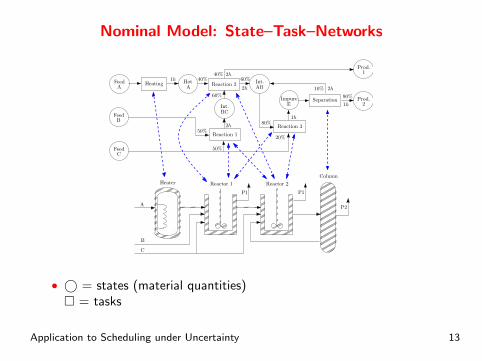
Nominal Model: State–Task–Networks

FeedA

Heating HotA

Reaction 2Int.AB

Reaction 3

ImpureE

Separation Prod.2

Prod.1

FeedB

FeedC

Reaction 1

Int.BC

Heater Reactor 1 Reactor 2

Column

1h

50%

50%

2h

40%

60%

60%

2h

40% 2h

20%

80%1h

90%

1h

10% 2h

A

B

C

P1 P1

P2

• © = states (material quantities)� = tasks


Explanations

• given: a set of physical units, a set of tasks that the units canperform and which transform states (material quantities), and aproduction network

• e.g., reactors 1 and 2 may perform reactions 1 2 and 3; reaction 2transforms a mix of states “hot A” and “intermediate BC” into thefinal product 1 and the intermediate state AB

• the scheduling problem is to establish what unit to assign to whichtask and at what time, in order to maximize a given performanceindex


STN Core Model

Variables:• xijt ∈ {0, 1} is 1 if unit i starts processing task j at time step t• ybatch

ijt , ystatest ∈ R batchsize and state (material) amount

Constraints (core):• unique unit allocation∑

j∈Jixijt ≤ 1∑

j∈Ji

∑t+Pj−1t′=t xijt′ − 1 ≤Mij(1− xijt) ∀i, t, j ∈ Ji

• capacity of processing units and storages

xijt · V minij ≤ ybatch

ijt ≤ xijt · V maxij ∀j, t, i ∈ Ij

0 ≤ ystatest ≤ Cs ∀s, t

• states update equations

ystatest = ystate

s,t−1+∑j∈Js

ρjs∑i∈Ij

ybatchij,t−Pjs

−∑j∈Js

ρjs∑i∈Ij

ybatchijt +Rst−Dst

• actual model may contain several “addon constraints”


Remarks on STNs

• generic model for scheduling batch production networks

• STNs and RTNs are very common in practice

• presented the discrete–time form

• continuous time formulation also exists (horrible eqns)

• “used to be” computationally intensive


Scheduling Uncertainty

• a number of sources of uncertainty affect schedules• time delays• unit malfunctioning or outage• natural events• human errors• unexpected changes in production requirements• . . .

• these have a substantial impact on the usefulness of a schedule

• issue is exacerbated by the fact that optimization routines tend to“pack” tasks at times when, e.g., prices are lowest

• how to handle?


Handling Uncertainty

Option 1:

• recompute a new schedule when event occurs (reactive)

• impractical, since the new schedule can be completely different

Option 2:

• use robust optimization to obtain flexible schedules

• these can support uncertain events without being disrupted

• and (optionally) allow for reactivity on y• stockpile size is regulated according to revealed uncertain events• while remaining within constraints


Modelling the Uncertainty – Example

• suppose that x? = [0, 1, 0, 0]>

• however, at planning time we do not know whether we will actuallybe able to implement x?

• e.g., a delay may result in

x = x? + w =

0100

+

0−110

• clearly, the value of w depends on the choice of x; andw = [0,−1, 1, 0] should only be active with x? = [0, 1, 0, 0] →W(x)

• on more complex decision problems, such a construction allows oneto encode a rich variety of uncertain events

• quantification from existing data conceptually easy: check thedifference between plan and actual execution to construct w


Experiments

FeedA

Heating HotA

Reaction 2Int.AB

Reaction 3

ImpureE

Separation Prod.2

Prod.1

FeedB

FeedC

Reaction 1

Int.BC

Heater Reactor 1 Reactor 2

Column

1h

50%

50%

2h

40%

60%

60%

2h

40% 2h

20%

80%1h

90%

1h

10% 2h

A

B

C

P1 P1

P2

1. heating delay by one hour

2. execution of reaction 2 may be swapped from reactor 1 to reactor 2,but only after the first four hours


Heating Delay – Nominal vs Robust

0 2 4 6 8 10

R

Separation

N

R

Reactor 2

N

R

Reactor 1

N

R

Heater

N

t

Nominal Obj.: 2744.4, Robust Obj.: 2744.4

H.

52

Rea.1

76

Rea.1

50

Rea.2

80

Rea.2

50

H.

32

Rea.2

80

Rea.3

50

Rea.3

14

Sep.

50

Rea.1

78

Rea.3

50

H.

52

Rea.3

50

Rea.2

80

Rea.2

50

Sep.

114

H.

100

Rea.1

76

Rea.1

50

Rea.2

80

Rea.2

50

H.

36

Rea.2

80

Rea.3

50

Rea.3

14

Sep.

50

Rea.1

78

Rea.3

50

Rea.3

50

Rea.2

80

Rea.2

50

Sep.

114


Heating Delay – Delay Occurred

0 2 4 6 8 10

R(w)

Separation

R(0)

R(w)

Reactor 2

R(0)

R(w)

Reactor 1

R(0)

R(w)

Heater

R(0)

t

H.

100

Rea.1

76

Rea.1

50

Rea.2

80

Rea.2

50

H.

36

Rea.2

80

Rea.3

50

Rea.3

14

Sep.

50

Rea.1

78

Rea.3

50

Rea.3

50

Rea.2

80

Rea.2

50

Sep.

114

Rea.1

76

Rea.1

50

H.

100

Rea.2

80

Rea.2

50

H.

36

Rea.2

80

Rea.3

50

Rea.3

14

Sep.

50

Rea.1

78

Rea.3

50

Rea.3

50

Rea.2

80

Rea.2

50

Sep.

114


Unit Swap – Nominal vs Robust

0 2 4 6 8 10

R

Separation

N

R

Reactor 2

N

R

Reactor 1

N

R

Heater

N

t

Nominal Obj.: 2744.4, Robust Obj.: 2513.8

H.

52

Rea.1

76

Rea.1

50

Rea.2

80

Rea.2

50

H.

32

Rea.2

80

Rea.3

50

Rea.3

14

Sep.

50

Rea.1

78

Rea.3

50

H.

52

Rea.3

50

Rea.2

80

Rea.2

50

Sep.

114

H.

100

Rea.1

80

Rea.1

50

Rea.2

80

Rea.2

50

H.

4

Rea.2

80

H.

12

Rea.1

44

Rea.3

78

Rea.3

80

Rea.2

80

Sep.

158


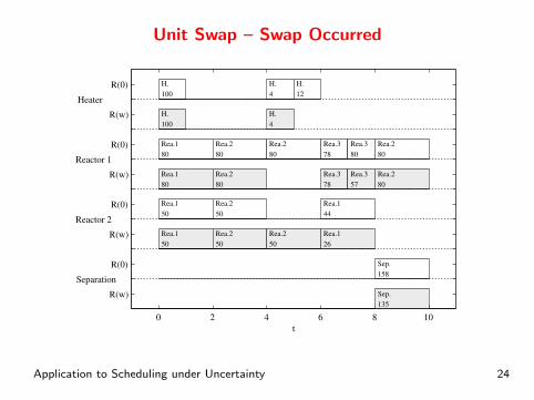
Unit Swap – Swap Occurred

0 2 4 6 8 10

R(w)

Separation

R(0)

R(w)

Reactor 2

R(0)

R(w)

Reactor 1

R(0)

R(w)

Heater

R(0)

t

H.

100

Rea.1

80

Rea.1

50

Rea.2

80

Rea.2

50

H.

4

Rea.2

80

H.

12

Rea.1

44

Rea.3

78

Rea.3

80

Rea.2

80

Sep.

158

H.

100

Rea.1

80

Rea.1

50

Rea.2

80

Rea.2

50

H.

4

Rea.2

50

Rea.1

26

Rea.3

78

Rea.3

57

Rea.2

80

Sep.

135


Further Remarks and Summary

The proposed method:

• is an approach to robust optimization that combines a preventiveand a reactive action

• can be used to generate flexible schedules

• allows the incorporation of a rich variety of events

• is more broadly applicable• not tied to any specific feature of STNs; application to other

scheduling systems possible• may be of use outside of scheduling altogether

• is computationally OK as far as we can tell• solve times for the STN examples: 0.4s for P, 1.1sec for RCP

• can be combined with existing techniques of robust optimization


Outline




Ongoing and Future Projects 26

Ongoing and Future Projects – Applications

• application of RO to scheduling models related to mining

• optimization of the energy management for large industrial loads

• “data driven optimization”


Ongoing and Future Projects – Theory

“Decomposition Methods for Large–Scale Non-Convex Models”:• previous work on large scale instances coupled through constraints

(e.g., shared resources)• applications: power systems control, supply chains (portfolio

optimization)• new: models coupled through variables (e.g., SIPs)

. . . . . .

• new insights on the tightness of decompositions based on duality• use of techniques based on ergodic sequences (averaging) for primal

recovery• use of new first-order methods (Nesterov)


Thank you for you attention!

Questions?


Counterexample

encode possible delay

of 1 unit by assuming

task A is length 2

the algorithm produces...


robust optimization of milps under decision dependent ... · pdf filerobust optimization of...

Documents