Time-Delay Estimation in Cognitive Radio and MIMO

Systems

a thesis

submitted to the department of electrical and

electronics engineering

and the institute of engineering and sciences

of bilkent university

in partial fulfillment of the requirements

for the degree of

master of science

By

Fatih Kocak

July 2010

I certify that I have read this thesis and that in my opinion it is fully adequate,

in scope and in quality, as a thesis for the degree of Master of Science.

Asst. Prof. Dr. Sinan Gezici (Supervisor)

I certify that I have read this thesis and that in my opinion it is fully adequate,

in scope and in quality, as a thesis for the degree of Master of Science.

Assoc. Prof. Dr. Ezhan Karasan

I certify that I have read this thesis and that in my opinion it is fully adequate,

in scope and in quality, as a thesis for the degree of Master of Science.

Asst. Prof. Dr. Ibrahim Korpeoglu

Approved for the Institute of Engineering and Sciences:

Prof. Dr. Levent OnuralDirector of Institute of Engineering and Sciences

ii

ABSTRACT

Time-Delay Estimation in Cognitive Radio and MIMO

Systems

Fatih Kocak

M.S. in Electrical and Electronics Engineering

Supervisor: Asst. Prof. Dr. Sinan Gezici

July 2010

In this thesis, the time-delay estimation problem is studied for cognitive radio

systems, multiple-input single-output (MISO) systems, and cognitive single-input

multiple-output (SIMO) systems. A two-step approach is proposed for cognitive

radio and cognitive SIMO systems in order to perform time-delay estimation with

significantly lower computational complexity than the optimal maximum likeli-

hood (ML) estimator. In the first step of this two-step approach, an ML estimator

is used for each receiver branch in order to estimate the unknown parameters of

the signal received via that branch. Then, in the second step, the estimates from

the first step are combined in various ways in order to obtain the final time-delay

estimate. The combining techniques that are used in the second step are called

optimal combining, signal-to-noise ratio (SNR) combining, selection combining,

and equal combining. It is shown that the performance of the optimal combining

technique gets very close to the Cramer-Rao lower bound (CRLB) at high SNRs.

iii

These combining techniques provide various mechanisms for diversity combining

for time-delay estimation and extend the concept of diversity in communications

systems to the time-delay estimation problem in cognitive radio and cognitive

SIMO systems. Simulation results are presented to evaluate the performance of

the proposed estimators and to verify the theoretical analysis. For the solution

of the time-delay estimation problem in MISO systems, ML estimation based on

a genetic global optimization algorithm, namely, differential evolution (DE), is

proposed. This approach is proposed in order to decrease the computational com-

plexity of the ML estimator, which results in a complex optimization problem in

general. A theoretical analysis is carried out by deriving the CRLB. Simulation

studies for Rayleigh and Rician fading scenarios are performed to investigate the

performance of the proposed algorithm.

Keywords: Time-delay estimation, cognitive radio, multiple-input single-output

(MISO) systems, cognitive single-input multiple-output (SIMO) systems, differ-

ential evolution (DE), maximum likelihood (ML) estimator, Cramer-Rao lower

bound (CRLB).

iv

OZET

BILISSEL RADYO SISTEMLERINDE VE COK GIRISLI COK

CIKISLI SISTEMLERDE ZAMAN GECIKMESI KESTIRIMI

Fatih Kocak

Elektrik ve Elektronik Muhendisligi Bolumu Yuksek Lisans

Tez Yoneticisi: Yrd. Doc. Dr. Sinan Gezici

Temmuz 2010

Bu tezde, bilissel radyo sistemleri, cok girisli tek cıkıslı sistemler ve bilissel tek

girisli cok cıkıslı sistemlerde zaman gecikmesi kestirimi problemi calısılmaktadır.

Bilissel radyo sistemlerinde ve bilissel tek girisli cok cıkıslı sistemlerde ideal

en buyuk olabilirlik kestiricisinden onemli derecede daha dusuk bir berimsel

karmasıklıkla zaman gecikmesi kestirimi yapmak amacıyla iki asamalı bir yaklasım

onerilmektedir. Bu onerilen iki asamalı yaklasımın ilk asamasında, her alıcı dalı

icin o dal yoluyla alınan sinyale ait bilinmeyen parametreleri kestirmek amacıyla

bir en buyuk olabilirlik kestiricisi kullanılmaktadır. Sonra, ikinci asamada, bi-

rinci asamada elde edilen tahminler son zaman gecikmesi tahminini elde et-

mek amacıyla cesitli yollarla birlestirilmektedir. Ideal birlestirme, sinyal gurultu

oranlı birlestirme, secici birlestirme ve esit birlestirme ikinci asamada kullanılan

birlestirme teknikleridir. Ideal birlestirme tekniginin performansının yuksek sinyal

gurultu oranlarında Cramer-Rao alt sınırına cok yaklastıgı gosterilmektedir. Bu

v

birlestirme teknikleri zaman gecikmesi kestirimine yonelik cesitleme birlestirme

icin bircok mekanizma sunmaktadır ve haberlesme sistemlerindeki cesitlilik kon-

septini bilissel radyo sistemlerinde ve bilissel tek girisli cok cıkıslı sistemlerde

zaman gecikmesi kestirimi problemine genisletmektedir. Onerilen kestiricilerin

performansını degerlendirmek ve teorik analizi dogrulamak amacıyla benzetim

sonucları sunulmaktadır. Cok girisli tek cıkıslı sistemlerdeki zaman gecikmesi ke-

stirimi probleminin cozumu icin bir global eniyileme algoritması olan diferansiyel

gelisim tabanlı en buyuk olabilirlik kestirimi one surulmektedir. Bu yaklasım,

genelde karmasık bir eniyileme problemiyle sonuclanan en buyuk olabilirlik kes-

tiricisinin berimsel karmasıklıgını azaltmak amacıyla one surulmektedir. Cramer-

Rao alt sınırı turetilerek bir teorik analiz yapılmaktadır. Onerilen algoritmanın

performansını incelemek amacıyla Rayleigh ve Rician sonumlenme senaryoları

icin benzetim calısmaları yapılmaktadır.

Anahtar Kelimeler: Zaman gecikmesi kestirimi, bilissel radyo, cok girisli tek

cıkıslı sistemler, bilissel tek girisli cok cıkıslı sistemler, diferansiyel gelisim, en

buyuk olabilirlik kestirimi, Cramer-Rao alt sınırı.

vi

ACKNOWLEDGMENTS

I would like to express my special thanks to my supervisor Asst. Prof. Dr. Sinan

Gezici whose guidance became a torch in my hands that enlightened my research

path and who turned the preparation of this thesis into fun.

I am grateful to Assoc. Prof. Dr. Ezhan Karasan and Asst. Prof. Dr.

Ibrahim Korpeoglu for their valuable contributions by taking place in my thesis

defense committee.

I would also like to thank Prof. H. Vincent Poor, Dr. Hasari Celebi, Prof.

Dr. Khalid A. Qaraqe, Prof. Dr. Huseyin Arslan, and Dr. Onay Urfalıoglu for

their precious contributions to my thesis.

My final gratitude is to my family, who did not hesitate to support me during

the preparation of this thesis, like in every step of my life.

vii

Contents

1 Introduction 1

1.2 Background . . . . . . . . . . . . . . . . . . . . . . . . . . . . . . 1

1.2.1 Cognitive Radio Systems . . . . . . . . . . . . . . . . . . . 1

1.2.2 Multiple-Input Multiple-Output Systems . . . . . . . . . . 2

1.2.3 Cognitive Multiple-Input Multiple-Output Systems . . . . 4

1.2.4 Positioning . . . . . . . . . . . . . . . . . . . . . . . . . . 4

1.3 Thesis Outline . . . . . . . . . . . . . . . . . . . . . . . . . . . . . 6

2 TIME-DELAY ESTIMATION IN DISPERSED SPECTRUM COG-

NITIVE RADIO SYSTEMS 8

2.1 Signal Model . . . . . . . . . . . . . . . . . . . . . . . . . . . . . 10

2.2 Optimal Time-Delay Estimation and Theoretical Limits . . . . . . 13

2.3 Two-Step Time-Delay Estimation and Diversity Combining . . . . 15

2.3.1 First Step: Parameter Estimation at Different Branches . . 16

2.3.2 Second Step: Combining Estimates from Different Branches 18

2.4 On the Optimality of Two-Step Time-Delay Estimation . . . . . . 21

2.5 Simulation Results . . . . . . . . . . . . . . . . . . . . . . . . . . 26

viii

3 TIME-DELAY ESTIMATION IN MULTIPLE-INPUT SINGLE-

OUTPUT SYSTEMS 34

3.1 Signal Model . . . . . . . . . . . . . . . . . . . . . . . . . . . . . 35

3.2 Theoretical Limits . . . . . . . . . . . . . . . . . . . . . . . . . . 36

3.3 ML Estimation Based On Differential Evolution . . . . . . . . . . 41

3.3.1 ML Estimator . . . . . . . . . . . . . . . . . . . . . . . . . 41

3.3.2 Differential Evolution (DE) . . . . . . . . . . . . . . . . . 41

3.4 Simulation Results . . . . . . . . . . . . . . . . . . . . . . . . . . 45

4 TIME-DELAY ESTIMATION IN COGNITIVE SINGLE-INPUT

MULTIPLE-OUTPUT SYSTEMS 49

4.1 Signal Model . . . . . . . . . . . . . . . . . . . . . . . . . . . . . 50

4.2 CRLB Calculations . . . . . . . . . . . . . . . . . . . . . . . . . . 52

4.3 CRLB Calculations for Single Band and Single Antenna Systems . 56

4.4 Two-Step Time-Delay Estimation . . . . . . . . . . . . . . . . . . 60

4.4.1 First Step: Maximum Likelihood Estimation at Each Branch 62

4.4.2 Second Step: Combining Time-Delay Estimates from Dif-

ferent Branches . . . . . . . . . . . . . . . . . . . . . . . . 63

4.5 Optimality of the Two-Step Estimator . . . . . . . . . . . . . . . 65

4.6 Simulation Results . . . . . . . . . . . . . . . . . . . . . . . . . . 67

5 Conclusions 79

A 82

B 85

ix

List of Figures

1.1 The structure of a cognitive radio system [11]. . . . . . . . . . . . 2

1.2 An example of opportunistic spectrum usage in a cognitive radio

network [14]. . . . . . . . . . . . . . . . . . . . . . . . . . . . . . . 3

1.3 An example of a MIMO system. . . . . . . . . . . . . . . . . . . . 3

2.1 Illustration of dispersed spectrum utilization in cognitive radio sys-

tems [22]. . . . . . . . . . . . . . . . . . . . . . . . . . . . . . . . 11

2.2 Block diagram of the front-end of a cognitive radio receiver, where

BPF and LNA refer to band-pass filter and low-noise amplifier,

respectively [22]. . . . . . . . . . . . . . . . . . . . . . . . . . . . 12

2.3 The block diagram of the proposed time-delay estimation approach.

The signals r1(t), . . . , rK(t) are obtained at the front-end of the re-

ceiver as shown in Figure 2.2. . . . . . . . . . . . . . . . . . . . . 16

2.4 RMSE versus SNR for the proposed algorithms, and the theoreti-

cal limit (CRLB). The signal occupies three dispersed bands with

bandwidths B1 = 200 kHz, B2 = 100 kHz and B3 = 400 kHz. . . . 27

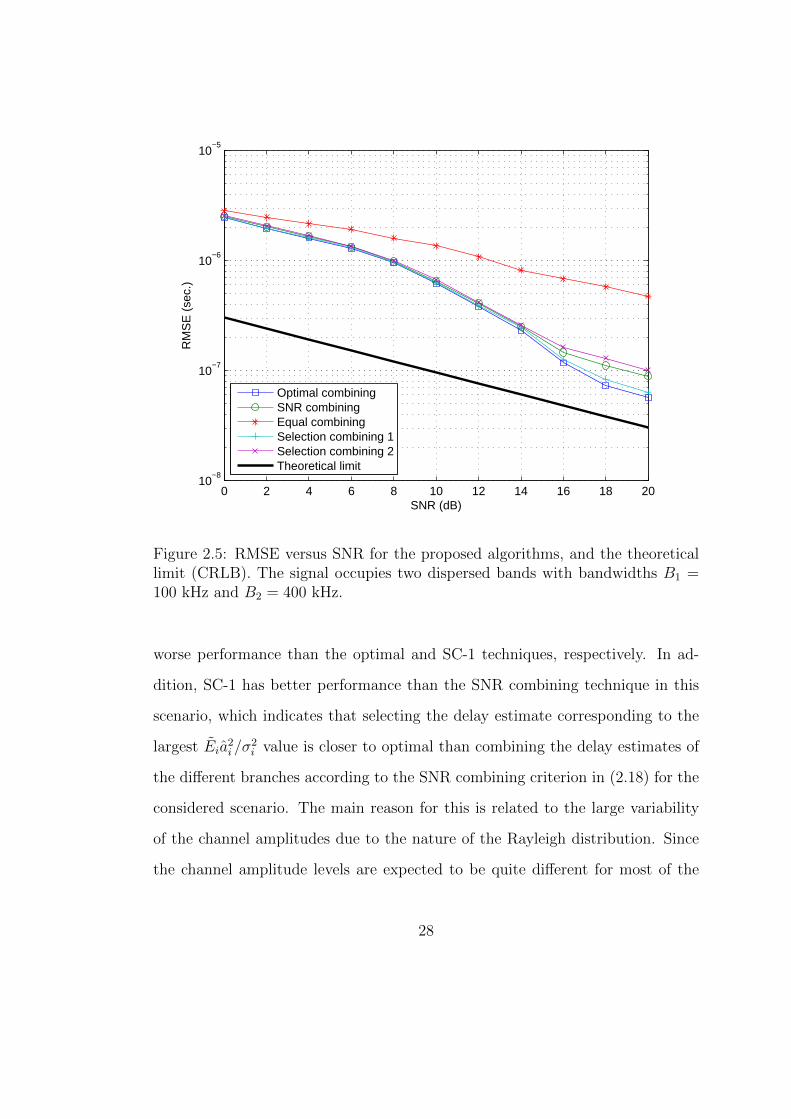
2.5 RMSE versus SNR for the proposed algorithms, and the theoret-

ical limit (CRLB). The signal occupies two dispersed bands with

bandwidths B1 = 100 kHz and B2 = 400 kHz. . . . . . . . . . . . 28

x

2.6 RMSE versus SNR for the proposed algorithms, and the theoretical

limit (CRLB). The signal occupies two dispersed bands with equal

bandwidths of 400 kHz. . . . . . . . . . . . . . . . . . . . . . . . . 30

2.7 RMSE versus the number of bands for the proposed algorithms,

and the theoretical limit (CRLB). Each band occupies 100 kHz,

and σ2i = 0.1 ∀i. . . . . . . . . . . . . . . . . . . . . . . . . . . . . 31

2.8 RMSE versus SNR for the proposed algorithms, and the theoretical

limit (CRLB) in the presence of CFO. The signal occupies two

dispersed bands with bandwidths B1 = 100 kHz and B2 = 400 kHz. 32

3.1 A MISO system with M transmitter antennas. . . . . . . . . . . . 35

3.2 The RMSE of the MLE and the square-root of the CRLB for the

Rayleigh fading channel. . . . . . . . . . . . . . . . . . . . . . . . 46

3.3 The RMSE of the MLE and the square-root of the CRLB for the

Rician fading channel (K = 5). . . . . . . . . . . . . . . . . . . . 47

4.1 SIMO structure. . . . . . . . . . . . . . . . . . . . . . . . . . . . . 50

4.2 Illustration of the two-step time-delay estimation algorithm for a

cognitive SIMO system. . . . . . . . . . . . . . . . . . . . . . . . 61

4.3 The performances of the estimators, RMSE vs. SNR, and the

theoretical limit (CRLB). There are 2 receive antennas, 3 dispersed

bands with 100 kHz, 200 kHz, and 400 kHz bandwidths under

Rayleigh fading condition. . . . . . . . . . . . . . . . . . . . . . . 68

4.4 The performances of the estimators, RMSE vs. SNR, and the

theoretical limit (CRLB). There are 2 receive antennas, 3 dispersed

bands each with 100 kHz bandwidth under Rayleigh fading condition. 69

xi

4.5 The performances of the estimators, RMSE vs. number of bands,

and the theoretical limit (CRLB). There are 2 receive antennas

under Rayleigh fading condition. . . . . . . . . . . . . . . . . . . . 71

4.6 The performances of the estimators, RMSE vs. number of anten-

nas, and the theoretical limit (CRLB). There are 3 dispersed bands

with 100 kHz, 200 kHz, and 400 kHz bandwidths under Rayleigh

fading condition. . . . . . . . . . . . . . . . . . . . . . . . . . . . 72

4.7 The performances of the estimators, RMSE vs. number of anten-

nas, and the theoretical limit (CRLB). There are 3 dispersed bands

each with 100 kHz bandwidth under Rayleigh fading condition. . . 73

4.8 The performances of the estimators, RMSE vs. SNR, and the

theoretical limit (CRLB). There are 2 receive antennas, 3 dispersed

bands with 100 kHz, 200 kHz, and 400 kHz bandwidths under

Rician fading condition. . . . . . . . . . . . . . . . . . . . . . . . 74

4.9 The performances of the estimators, RMSE vs. SNR, and the

theoretical limit (CRLB). There are 2 receive antennas, 3 dispersed

bands each with 100 kHz bandwidth under Rician fading condition. 75

4.10 The performances of the estimators, RMSE vs. number of bands,

and the theoretical limit (CRLB). There are 2 receive antennas

under Rician fading condition. . . . . . . . . . . . . . . . . . . . . 76

4.11 The performances of the estimators, RMSE vs. number of an-

tennas, and the theoretical limit (CRLB). There are 3 dispersed

bands with 100 kHz, 200 kHz, and 400 kHz bandwidths under

Rician fading condition. . . . . . . . . . . . . . . . . . . . . . . . 77

xii

4.12 The performances of the estimators, RMSE vs. number of anten-

nas, and the theoretical limit (CRLB). There are 3 dispersed bands

each with 100 kHz bandwidth under Rician fading condition. . . . 78

xiii

To Science and Scientists ...

Chapter 1

Introduction

1.2 Background

1.2.1 Cognitive Radio Systems

Cognitive radio is a promising approach to implement intelligent wireless com-

munications systems [1]-[8]. Cognitive radios can be perceived as more capable

versions of software defined radios in the sense that they have sensing, awareness,

learning, adaptation, goal driven autonomous operation and reconfigurability fea-

tures [9], [10]. In Figure 1.1, the basic functional blocks of a cognitive radio are

illustrated [11].

As a result of the aforementioned features of cognitive radio systems, radio

resources, such as power and bandwidth, can be used more efficiently [1]. Espe-

cially since the electromagnetic spectrum is a precious resource, it must not be

wasted. The recent spectrum measurement campaigns in the United States [12]

and Europe [13] show that the spectrum is under-utilized; hence, opportunistic

use of unoccupied frequency bands is highly desirable.

1

Figure 1.1: The structure of a cognitive radio system [11].

Cognitive radio provides a solution to the problem of inefficient spectrum

utilization by using the vacant frequency spectrum over time in a certain geo-

graphical region. In other words, a cognitive radio system can opportunistically

use the available spectrum of a legacy system without interfering with the licensed

users of that spectrum [2, 3]. An example of spectrum usage in a cognitive radio

network can be seen in Figure 1.2 [14].

1.2.2 Multiple-Input Multiple-Output Systems

A multiple-input multiple-output (MIMO) system uses multiple antennas at the

transmitter and the receiver in order to provide space diversity [15]. MIMO

2

Figure 1.2: An example of opportunistic spectrum usage in a cognitive radionetwork [14].

systems will be used very widely in future communications systems since they

provide advantages in terms of quality, reliability and capacity [15], [16]. An

example of a MIMO structure is depicted in Figure 1.3.

Figure 1.3: An example of a MIMO system.

Multiple-input single-output (MISO) systems, which are special cases of MIMO

3

systems, have multiple antennas at the transmitter but have a single antenna

at the receiver. In this case, the space diversity can be called as the transmit

diversity. Similarly, single-input multiple-output (SIMO) systems have a single

antenna at the transmitter side and multiple antennas at the receiver side. SIMO

systems also have space diversity, which can be called as receive diversity, since

their multiple antenna structure is at the receiver side.

1.2.3 Cognitive Multiple-Input Multiple-Output Systems

Employment of the MIMO structure in cognitive radio systems brings the space

diversity advantages of MIMO to cognitive radio networks [17], [18]. The resulting

system can be called a cognitive MIMO radio [19], [20]. There are a few studies

on cognitive radio MIMO networks, such as [21], since it is a relatively new topic

resulting from the mergence of two hot research topics.

In cognitive MIMO radio systems, diversity is utilized in 2 dimensions, which

are space and frequency. Space diversity results from the MIMO structure as

mentioned before. Frequency diversity is a consequence of the dispersed spec-

trum utilization feature of cognitive radios. A cognitive radio can detect the

vacant spectral bands at an arbitrary time and place. It can use multiple of

those frequency bands if they are available. Therefore, using multiple dispersed

frequency bands introduces frequency diversity to the cognitive radio system [22].

1.2.4 Positioning

Facilitating wireless networks in positioning applications besides the communica-

tions applications has been getting a growing attention recently [23]. There are

a lot of application areas and services that make use of positioning techniques.

4

The typical examples for outdoor systems are enhanced 911 (E911), improved

fraud detection, cellular system design and management, mobile yellow pages,

location-based billing, intelligent transport systems, improved transport systems

and the global positioning system (GPS) [24], [25]. For short-range networks

and indoor positioning systems, inventory tracking, intruder detection, tracking

of fire-fighters and miners, home automation and patient monitoring applications

are examples that employ wireless positioning techniques [26].

Since positioning is an important application area of wireless systems, it is im-

portant to quantify the advantages of space diversity, which is utilized in MIMO

systems, for positioning applications. Although the advantages of space diversity

are investigated thoroughly for communications purposes [27] and radar systems

[28], [29], [30], there are a few studies in the literature that investigate the ef-

fects of space diversity for positioning purposes. For example, [31] studies the

space diversity that can be obtained via the use of multiple receive antennas.

Mainly, it obtains the theoretical limits, in terms of the Cramer-Rao lower bound

(CRLB), on range (equivalently, time-delay) estimation, and proposes a two-step

asymptotically optimal range estimator.

It is mentioned in Section 1.2.1 that cognitive radios are able to facilitate op-

portunistic spectrum utilization. Therefore, it is important that cognitive radio

devices are aware of their positions and monitor the environment continuously.

These location and environmental awareness features of cognitive radios have

been studied extensively in the literature [10], [32]-[38]. In [32], the concept of

cognitive radar is introduced, which provides information related to the objects

in an environment; i.e., it performs environmental sensing. In [33], a radio en-

vironment mapping method for cognitive radio networks is studied. Conceptual

5

models for location and environmental awareness engines and cycles are proposed

in [10], [34] and [35] for cognitive radio systems. Also, [37] introduces the con-

cept of a topology engine for cognitive radios by studying topology information

characterization and its applications to cognitive radio networks. The location

awareness feature of cognitive radios can also be used in many network opti-

mization applications, such as location-assisted spectrum management, network

planning, handover, routing, dynamic channel allocation and power control [8],

[39].

1.3 Thesis Outline

In Chapter 2, the time-delay estimation problem in cognitive radio systems is

analyzed. In Section 2.1, the signal model is introduced and the signal at each

branch of the receiver is described. In Section 2.2, the optimal ML receiver is

obtained, and the CRLBs on time delay estimation in dispersed spectrum cogni-

tive radio systems are described. The proposed two-step time delay estimation

approach is studied in Section 2.3. Then, in Section 2.4, the optimality proper-

ties of the proposed time delay estimators are investigated. Finally, simulation

results are presented in Section 2.5.

In Chapter 3, the analysis of the time-delay estimation problem in MISO sys-

tems is performed. First, the signal model is constructed in Section 3.1. Then,

the maximum likelihood (ML) time-delay estimator is provided and a theoretical

analysis is performed in Section 3.2 by deriving the CRLB on time-delay estima-

tion in a MISO system. In Section 3.3, a genetic global optimization algorithm,

called differential evolution (DE), is used to estimate the time-delay parameter

6

from the ML estimator formulation. In that way, the CRLB can be achieved at

high SNRs with a significantly lower computational complexity than the direct

solution of the ML estimator via an exhaustive search. In DE, a number of pa-

rameter vectors are generated and updated at each generation in order to reach

the global optimum [40], and these vectors encounter mutation, crossover, and

selection steps at each generation [41]. Finally, simulation results are presented.

In Chapter 4, the time-delay estimation problem in cognitive SIMO systems

is analyzed. This part of the thesis starts with the signal model in Section

4.1. Then, in Section 4.2, the theoretical bound for the estimation of the time-

delay parameter after determining the log-likelihood function and the unknown

parameters. Next, a two-step time-delay estimation algorithm is proposed, which

is similar to the one proposed for cognitive radio systems in Chapter 2. This two-

step approach includes ML estimation in every receiver branch and combination

of the time-delay estimates of each branch in various ways in order to find the

final time-delay estimate. In Section 4.6, the simulation results are provided.

7

Chapter 2

TIME-DELAY ESTIMATION

IN DISPERSED SPECTRUM

COGNITIVE RADIO SYSTEMS

Location awareness requires that a cognitive radio device performs accurate esti-

mation of its position. One possible way of obtaining position information is to

use the Global Positioning System (GPS) technology in cognitive radio systems.

However, this is not a very efficient or cost-effective solution [36]. As another ap-

proach, cognitive radio devices can estimate position related parameters of signals

traveling between them in order to estimate their positions [36], [23]. Among var-

ious position related parameters, the time-delay parameter commonly provides

accurate position information with reasonable complexity [23], [42]. The main

focus of Chapter 2 is time-delay estimation in cognitive radio systems. In other

words, the aim is to propose techniques for accurate time-delay estimation in

dispersed spectrum systems in order to provide accurate location information to

8

cognitive users. Since the accuracy of location estimation increases as the accu-

racy of time-delay estimation increases, design of time-delay estimators with high

accuracy and reasonable complexity is crucial for the location awareness feature

of a cognitive radio system [23].

Time-delay estimation in cognitive radio systems differs from conventional

time-delay estimation mainly due to the fact that a cognitive radio system can

transmit and receive over multiple dispersed bands. In other words, since a cog-

nitive radio device can utilize the spectral holes of a legacy system, it can have a

spectrum that consists of multiple bands that are dispersed over a wide range of

frequencies (cf. Figure 2.1). In [43], the theoretical limits on time-delay estima-

tion are studied for dispersed spectrum cognitive radio systems, and the effects

of carrier frequency offset (CFO) and modulation schemes of training signals on

the accuracy of time-delay estimation are quantified. The expressions for the

theoretical limits indicate that frequency diversity can be utilized in time-delay

estimation. Similarly, the effects of spatial diversity on time-delay estimation

are studied in [31] for single-input multiple-output (SIMO) systems. In addition,

the effects of multiple antennas on time-delay estimation and synchronization

problems are investigated in [44].

In this chapter, time-delay estimation is studied for dispersed spectrum cog-

nitive radio systems. First, it is observed that maximum likelihood (ML) esti-

mation is not very practical for time-delay estimation in such systems. Then, a

two-step time-delay estimation approach is proposed in order to provide accurate

time-delay estimation with significantly lower computational complexity than

that of the optimal ML estimator. In the proposed scheme, the receiver consists

of multiple branches and each branch processes the part of the received signal

9

that occupies the corresponding frequency band. An ML estimator is used in

each branch in order to estimate the unknown parameters of the signal observed

in that branch. Then, in the second step, the estimates from all the branches

are combined to obtain the final time-delay estimate. Various techniques are

proposed for the combining operation in the second step: Optimal combining,

signal-to-noise ratio (SNR) combining, selection combining, and equal combin-

ing. The biases and variances of the time-delay estimators that employ these

combining techniques are investigated. It is shown that the optimal combining

technique results in a mean-squared error (MSE) that approximates the Cramer-

Rao lower bound (CRLB) at high SNRs. Simulation results are provided in order

to compare the performance of the proposed time-delay estimators. In a more

generic perspective, this study focuses on the utilization of frequency diversity

for a parameter estimation problem. Therefore, the proposed estimators can be

applied to other systems that have frequency diversity as well.

2.1 Signal Model

A cognitive radio system that occupies K dispersed frequency bands is considered

as shown in Figure 2.1. The transmitter sends a signal occupying all the K bands

simultaneously, and the receiver aims to calculate the time-delay of the incoming

signal [45].

One approach for designing such a system involves the use of orthogonal fre-

quency division multiplexing (OFDM). In this approach, the received signal is

considered as a single OFDM signal with zero coefficients at the sub-carriers

10

Frequency….

PSDfc1 fc2 fcKB1 BKB2

UnavailableBandsFigure 2.1: Illustration of dispersed spectrum utilization in cognitive radio sys-tems [22].

corresponding to the unavailable bands [46]-[48]. Then, the signal can be pro-

cessed as in conventional OFDM receivers. The main drawback of this approach

is that it requires processing of very large bandwidths when the available spec-

trum is dispersed over a wide range of frequencies. Therefore, the design of RF

components, such as filters and low-noise amplifiers (LNAs) can become very

complex and costly, and result in components with high power consumption [25].

In such scenarios, it can be more practical to process the received signal in mul-

tiple branches, as shown in Figure 2.2. In that case, each branch processes one

available band, and down-converts the signal according to the center frequency

of that band. Therefore, signals with narrower bandwidths can be processed at

each branch [22].

11

fc1B1PSD ffc2B2PSD f

fcKBKPSD f... ...

r1(t)fc1r2(t)fc2rK(t)fcK

DownconversionLNABPF1DownconversionLNABPF2DownconversionLNABPFK

Figure 2.2: Block diagram of the front-end of a cognitive radio receiver, whereBPF and LNA refer to band-pass filter and low-noise amplifier, respectively [22].

12

For the receiver model in Figure 2.2, the baseband representation of the re-

ceived signal in the ith branch can be modeled as

ri(t) = αi ejωitsi(t− τ) + ni(t) , (2.1)

for i = 1, . . . , K, where τ is the time-delay of the signal, αi = ai ejφi and ωi

represent, respectively, the channel coefficient and the CFO for the signal in the

ith branch, si(t) is the baseband representation of the transmitted signal in the

ith band, and ni(t) is modeled as complex white Gaussian noise with independent

components, each having spectral density σ2i .

The signal model in (2.1) assumes that the signal in each branch can be

modeled as a narrowband signal. Hence, a single complex channel coefficient is

used to represent the fading of each signal.

The system model considered in this study falls within the framework of cog-

nitive radio systems, since the cognitive user first needs to detect the available fre-

quency bands, and then to adapt its receiver parameters accordingly. Therefore,

the spectrum sensing and adaptation features of cognitive systems are assumed

for the considered system in this study [9], [10].

2.2 Optimal Time-Delay Estimation and Theo-

retical Limits

Accurate estimation of the time-delay parameter τ in (2.1) is quite challenging

due to the presence of unknown channel coefficients and CFOs. For a system

with K bands, there are 3K nuisance parameters. In other words, the vector θ

13

of unknown parameters can be expressed as

θ = [τ a1 · · · aK φ1 · · ·φK ω1 · · ·ωK ] . (2.2)

When the signals in (2.1) are observed over the interval [0, T ], the log-likelihood

function for θ is given by [49]

Λ(θ) = c−K∑i=1

1

2σ2i

∫ T

0

∣∣ri(t)− αi ejωitsi(t− τ)∣∣2 dt , (2.3)

where c is a constant that is independent of θ (the unknown parameters are

assumed to be constant during the observation interval). Then, the ML estimate

for θ can be obtained from (2.3) as [43]

θML = arg maxθ

{K∑i=1

1

σ2i

∫ T

0

R{α∗i e

−jωitri(t)s∗i (t− τ)

}dt−

K∑i=1

Ei|αi|2

2σ2i

},

(2.4)

where Ei =∫ T0|si(t− τ)|2dt is the signal energy, and R represents the operator

that selects the real-part of its argument.

It is observed from (2.4) that the ML estimator requires an optimization over

a (3K + 1)-dimensional space, which is quite challenging in general. Therefore,

the aim of this study is to propose low-complexity time-delay estimation algo-

rithms with comparable performance to that of the ML estimator in (2.4). In

other words, accurate time-delay estimation algorithms are studied under prac-

tical constraints on the processing power of the receiver. Since the ML estimator

is difficult to implement, the performance comparisons will be performed with

respect to the theoretical limits on time-delay estimation (of course, an ML esti-

mator achieves the CRLB asymptotically under certain conditions [49]). In [43],

the CRLBs on the mean-squared errors (MSEs) of unbiased time-delay estimators

14

are obtained for the signal model in (2.1). When the baseband representation of

the signals in different branches are of the form si(t) =∑

l di,lpi(t − lTi), where

di,l denotes the complex training data and pi(t) is a pulse with duration Ti, the

CRLB is expressed as

E{(τ − τ)2} ≥

(K∑i=1

a2iσ2i

(Ei − (ER

i )2/Ei

))−1, (2.5)

where

Ei =

∫ T

0

|s′i(t− τ)|2dt , (2.6)

and

ERi =

∫ T

0

R{s′i(t− τi)s∗i (t− τi)}dt , (2.7)

with s′(t) representing the first derivative of s(t). In the special case of |di,l| = |di|

∀l and pi(t) satisfying pi(0) = pi(Ti) for i = 1, . . . , K, (2.5) becomes [43]

E{(τ − τ)2} ≥

(K∑i=1

Ei a2i

σ2i

)−1. (2.8)

It is observed from (2.5) and (2.8) that frequency diversity can be useful in time-

delay estimation. For example, when one of the bands is in a deep fade ( i.e.,

small a2i ), some other bands can still be in good condition to facilitate accurate

time-delay estimation.

2.3 Two-Step Time-Delay Estimation and Di-

versity Combining

Due to the complexity of the ML estimator in (2.4), a two-step time-delay es-

timation approach is proposed in this study, as shown in Figure 2.3. Two-step

15

approaches are commonly used in optimization/estimation problems in order to

provide suboptimal solutions with reduced computational complexity [50, 51].

In the proposed estimator, each branch of the receiver performs estimation of

the time-delay, the channel coefficient and the CFO related to the signal in that

branch. Then, the estimates from all the branches are used to obtain the final

time-delay estimate as shown in Figure 2.3. In the following sections, the details

of the proposed approach are explained, and the utilization of frequency diversity

in time-delay estimation is explained.

Figure 2.3: The block diagram of the proposed time-delay estimation approach.The signals r1(t), . . . , rK(t) are obtained at the front-end of the receiver as shownin Figure 2.2.

2.3.1 First Step: Parameter Estimation at Different Branches

In the first step of the proposed approach, the unknown parameters of each re-

ceived signal are estimated at the corresponding receiver branch according to the

16

ML criterion (cf. Figure 2.3). Based on the signal model in (2.1), the likelihood

function at branch i can be expressed as

Λi(θi) = ci −1

2σ2i

∫ T

0

∣∣ri(t)− αi ejωitsi(t− τ)∣∣2 dt , (2.9)

for i = 1, . . . , K, where θi = [τ ai φi ωi] represents the vector of unknown

parameters related to the signal at the ith branch, ri(t), and ci is a constant that

is independent of θi.

From (2.9), the ML estimator at branch i can be stated as

θi = arg minθi

∫ T

0

∣∣ri(t)− αi ejωitsi(t− τ)∣∣2 dt , (2.10)

where θi = [τi ai φi ωi] is the vector of estimates at the ith branch. After some

manipulation, the solution of (2.10) can be obtained as[τi φi ωi

]= arg max

φi,ωi,τi

∣∣∣∣∫ T

0

R{ri(t) e−j(ωit+φi)s∗i (t− τi)

}dt

∣∣∣∣ (2.11)

and

ai =1

Ei

∫ T

0

R{ri(t) e−j(ωit+φi)s∗i (t− τi)

}dt . (2.12)

In other words, at each branch, optimization over a three-dimensional space is

required to obtain the unknown parameters. Compared to the ML estimator in

Section 2.2, the optimization problem in (2.4) over (3K + 1) variables is reduced

to K optimization problems over three variables, which results in a significant

amount of reduction in the computational complexity.

In the absence of CFO; i.e., ωi = 0 ∀i, (2.11) and (2.12) reduce to[τi φi

]= arg max

φi,τi

∣∣∣∣∫ T

0

R{ri(t) e−jφis∗i (t− τi)

}dt

∣∣∣∣ (2.13)

17

and

ai =1

Ei

∫ T

0

R{ri(t) e−jφis∗i (t− τi)

}dt . (2.14)

In that case, the optimization problem at each branch is performed over only

two dimensions. This scenario is valid when the carrier frequency of each band

is known accurately.

2.3.2 Second Step: Combining Estimates from Different

Branches

After obtaining K different time-delay estimates, τ1, . . . , τK , in (2.11), the second

step combines those estimates according to one of the criteria below and makes

the final time-delay estimate (cf. Figure 2.3).

Optimal Combining

According to the “optimal” combining criterion (the optimality properties of this

combining technique are investigated in Section 2.4), the time-delay estimate is

obtained as

τ =

∑Ki=1 κi τi∑Ki=1 κi

, (2.15)

where τi is the time-delay estimate of the ith branch, which is obtained from

(2.11), and

κi =a2i Eiσ2i

, (2.16)

with Ei being defined in (2.6). In other words, the optimal combining technique

estimates the time-delay as a weighted average of the time-delays of different

18

branches, where the weights are chosen as proportional to the multiplication of

the SNR estimate, Eia2i /σ

2i , and Ei/Ei . Since Ei is defined as the energy of

the first derivative of si(t) as in (2.6), Ei/Ei can be expressed, using Parseval’s

relation, as Ei/Ei = 4π2β2i , where βi is the effective bandwidth of si(t), which is

defined as [49]

β2i =

1

Ei

∫ ∞−∞

f 2|Si(f)|2df , (2.17)

with Si(f) denoting the Fourier transform of si(t). Therefore, it is concluded that

the optimal combining technique assigns a weight to the time-delay estimate

of a given branch in proportion to the product of the SNR estimate and the

effective bandwidth related to that branch. The intuition behind this combining

technique is the fact that signals with larger effective bandwidths and/or larger

SNRs facilitate more accurate time-delay estimation [49]; hence, their weights

should be larger in the combining process. This intuition is verified theoretically

in Section 2.4.

SNR Combining

The second technique combines the time-delay estimates in the first step ac-

cording to the SNR estimates at the respective branches. In other words, the

time-delay estimate is obtained as

τ =

∑Ki=1 γi τi∑Ki=1 γi

, (2.18)

where

γi =a2iEiσ2i

. (2.19)

19

Note that γi defines the SNR estimate at branch i. In other words, this technique

considers only the SNR estimates at the branches in order to determine the

combining coefficients, and does not take the signal bandwidths into account.

It is observed from (2.15)-(2.19) that the optimal combining and the SNR

combining techniques become equivalent if E1/E1 = · · · = EK/EK . Since

Ei/Ei = 4π2β2i , where βi is the effective bandwidth defined in (2.17), the two

techniques are equivalent when the effective bandwidths of the signals at differ-

ent branches are all equal.

Selection Combining-1 (SC-1)

Another technique for obtaining the final time-delay estimate is to determine the

“best” branch and to use its estimate as the final time-delay estimate. According

to SC-1, the best branch is defined as the one that has the maximum value of

κi = a2i Ei/σ2i for i = 1, . . . , K. In other words, the branch with the maximum

multiplication of the SNR estimate and the effective bandwidth is determined as

the best branch and its estimate is used as the final one. That is,

τ = τm , m = arg maxi∈{1,...,K}

{a2i Ei/σ

2i

}, (2.20)

where τm represents the time-delay estimate at the mth branch.

Selection Combining-2 (SC-2)

Similar to SC-1, SC-2 selects the “best” branch and uses its estimate as the final

time-delay estimate. However, according to SC-2, the best branch is defined as

the one with the maximum SNR. Therefore, the time-delay estimate is obtained

20

as follows according to SC-2:

τ = τm , m = arg maxi∈{1,...,K}

{a2iEi/σ

2i

}, (2.21)

where τm represents the time-delay estimate at the mth branch.

SC-1 and SC-2 become equivalent when the effective bandwidths of the signals

at different branches are all equal.

Equal Combining

The equal combining technique assigns equal weights to the estimates from dif-

ferent branches and obtains the time-delay estimate as follows:

τ =1

K

K∑i=1

τi . (2.22)

Considering the proposed combining techniques above, it is observed that

they are similar to diversity combining techniques in communications systems

[52]. However, the main difference is the following. The aim is to maximize the

SNR or to reduce the probability of symbol error in communications systems [52],

whereas, in the current problem, it is to reduce the MSE of time-delay estimation.

In other words, this study considers diversity combining for time-delay estimation,

where the diversity results from the dispersed spectrum utilization of the cognitive

radio system [22].

2.4 On the Optimality of Two-Step Time-Delay

Estimation

In this section, the asymptotic optimality properties of the two-step time-delay

estimators proposed in the previous section are investigated. In order to analyze

21

the performance of the estimators at high SNRs, the result in [31] for time-delay

estimation at multiple receive antennas is extended to the scenario in this study.

Lemma 1: Consider any linear modulation of the form si(t) =∑

l di,lpi(t−

lTi), where di,l denotes the complex data for the lth symbol of signal i, and pi(t)

represents a pulse with duration Ti. Assume that∫∞−∞ s

′i(t− τ)s∗i (t− τ)dt = 0 for

i = 1, . . . , K. Then, for the signal model in (2.1), the delay estimate in (2.11)

and the channel amplitude estimate in (2.12) can be modeled, at high SNR, as

τi = τ + νi , (2.23)

ai = ai + ηi , (2.24)

for i = 1, . . . , K, where νi and ηi are independent zero mean Gaussian random

variables with variances σ2i /(Ei a

2i ) and σ2

i /Ei, respectively. In addition, νi and

νj (ηi and ηj) are independent for i 6= j.

Proof: The proof uses the derivations in [43] in order to extend Lemma 1 in

[31] to the cases with CFO. At high SNRs, the ML estimate θi of θi = [τ ai φi ωi]

in (2.11) and (2.12) is approximately distributed as a jointly Gaussian random

variable with the mean being equal to θi and the covariance matrix being given by

the inverse of the Fisher information matrix (FIM) for observation ri(t) in (2.1)

over [0, T ]. Then, the results in [43] can be used to show that, under the conditions

in the lemma, the first 2 × 2 block of the covariance matrix can be obtained as

diag{σ2i /(Eia

2i ), σ

2i /Ei}. Therefore, τi and ai can be modeled as in (2.23) and

(2.24). In addition, since the noise at different branches are independent, the

estimates are independent for different branches. �

Based on Lemma 1, the asymptotic unbiasedness properties of the estima-

tors in Section 2.3 can be verified. First, it is observed from Lemma 1 that

E{τi} = τ . Considering the optimal combining technique in (2.15) as example,

22

the unbiasedness property can be shown as

E{τ |a1, . . . , aK} =

∑Ki=1 κi E{τi|a1, . . . , aK}∑K

i=1 κi=

∑Ki=1 κi E{τi|ai}∑K

i=1 κi= τ , (2.25)

where κi = a2i Ei/σ2i . Since E{τ |a1, . . . , aK} does not depend on a1, . . . , aK ,

E{τ} = E{E{τ |a1, . . . , aK}} = τ . In other words, since for each specific value

of ai, τi is unbiased (i = 1, . . . , K), the weighted average of τ1, . . . , τK is also

unbiased. Similar arguments can be used to show that all the two-step estimators

described in Section 2.3 are asymptotically unbiased.

Regarding the variance of the estimators, it can be shown that the optimal

combining technique has a variance that is approximately equal to the CRLB at

high SNRs (in fact, this is the main reason why this combining technique is called

optimal). To that aim, the conditional variance of τ in (2.15) given a1, . . . , aK is

obtained as follows:

Var{τ |a1, . . . , aK} =

∑Ki=1 κ

2i Var{τi|a1, . . . , aK}(∑K

i=1 κi

)2 , (2.26)

where the independence of the time-delay estimates is used to obtain the result

(cf. Lemma 1). Since Var{τi|a1, . . . , aK} = Var{τi|ai} = σ2i /(Ei a

2i ) from Lemma

1 and κi = a2i Ei/σ2i , (2.26) can be expressed as

Var{τ |a1, . . . , aK} =

∑Ki=1

a4i E2i

σ4i

σ2i

Eia2i(∑Ki=1

a2i Ei

σ2i

)2=

K∑i=1

a4i Eia2iσ

2i

(K∑i=1

a2i Eiσ2i

)−2. (2.27)

Lemma 1 states that at high SNRs, ai is distributed as a Gaussian random

variable with mean ai and variance σ2i /Ei . Therefore, for sufficiently large values

23

of Ei

σ2i, . . . , EK

σ2K

, (2.27) can be approximated by

Var{τ |a1, . . . , aK} ≈

(K∑i=1

Ei a2i

σ2i

)−1, (2.28)

which is equal to CRLB expression in (2.8). Therefore, the optimal combining

technique in (2.15) results in an approximately optimal estimator at high SNRs.

The variances of the other combining techniques in Section 2.3 can be obtained

in a straightforward manner and it can be shown that the asymptotic variances

are larger than the CRLB in general. For example, for the SNR combining

technique in (2.18), the conditional variance can be calculated as

Var{τ |a1, . . . , aK} =

∑Ki=1

a4iE2i

σ4i

σ2i

Eia2i(∑Ki=1

a2iEi

σ2i

)2=

K∑i=1

a4iE2i

a2i Eiσ2i

(K∑i=1

a2iEiσ2i

)−2, (2.29)

which, for sufficiently large SNRs, becomes

Var{τ |a1, . . . , aK} ≈K∑i=1

a2iE2i

Eiσ2i

(K∑i=1

a2iEiσ2i

)−2. (2.30)

Then, from the Cauchy-Schwarz inequality, the following condition is obtained:

Var{τ |a1, . . . , aK} ≈

∑Ki=1

a2iE2i

Eiσ2i(∑K

i=1aiEi

σi

√Ei

ai

√Ei

σi

)2 ≥

∑Ki=1

a2iE2i

Eiσ2i∑K

i=1a2iE

2i

Eiσ2i

∑Ki=1

a2i Ei

σ2i

= CRLB ,

(2.31)

which holds with equality if and only if E1

E1= · · · = EK

EK(or, β1 = · · · = βK).

In fact, under that condition, the optimal combining and the SNR combining

techniques become identical as mentioned in Section 2.3, since κi = a2i Ei/σ2i =

(Ei/Ei)(Eia2i /σ

2i ) = (Ei/Ei)γi (cf. (2.16) and (2.19)). In other words, when

24

the effective bandwidths of the signals at different branches are not equal, the

asymptotic variance of the SNR combining technique is strictly larger than the

CRLB.

Regarding the selection combining approaches in (2.20) and (2.21), similar

conclusions as for the diversity combining techniques in communications systems

can be made [52]. Specifically, SC-1 and SC-2 perform worse than the optimal

combining and the SNR combining techniques, respectively, in general. However,

when the estimate of a branch is significantly more accurate than the others, the

performance of the selection combining approach can get very close to the opti-

mal combining or the SNR combining technique. However, when the branches

have similar estimation accuracies, the selection combining techniques can per-

form significantly worse. The conditional variances of the selection combining

techniques can be approximated at high SNR as

Var{τ |a1, . . . , aK} ≈ min

{σ21

E1a21, . . . ,

σ2K

EKa2K

}, (2.32)

for SC-1, and

Var{τ |a1, . . . , aK} ≈Em

Emmin

{σ21

E1a21, . . . ,

σ2K

EKa2K

}, (2.33)

for SC-2, where m = arg mini∈{1,...,K}

{σ2i /(Eia

2i )} . From (2.32) and (2.33), it is

observed that if E1

E1= · · · = EK

EK(β1 = · · · = βK), then the asymptotic variances

of the SC-1 and SC-2 techniques become equivalent.

Finally, for the equal combining technique, the variance can be obtained from

(2.22) as

Var{τ} =1

K2

K∑i=1

σ2i

Eia2i. (2.34)

25

In general, the equal combining technique is expected to have the worst perfor-

mance since it does not make use of any information about the SNR or the signal

bandwidths in the estimation of the time-delay.

2.5 Simulation Results

In this section, simulations are performed in order to evaluate the performance

of the proposed time-delay estimators and compare them with each other and

against the CRLBs. The signal si(t) in (2.1) corresponding to each branch is

modeled by the Gaussian doublet given by

si(t) = Ai

(1− 4π(t− 1.25 ζi)

2

ζ2i

)e−2π(t−1.25ζi)

2/ζ2i , (2.35)

where Ai and ζi are the parameters that are used to adjust the pulse energy and

the pulse width, respectively. The bandwidth of si(t) in (2.35) can approximately

be expressed as Bi ≈ 1/(2.5 ζi) [25]. For the following simulations, Ai values are

adjusted to generate unit-energy pulses.

For all the simulations, the spectral densities of the noise at different branches

are assumed to be equal; that is, σ2i = σ2 for i = 1, . . . , K. In addition, the SNR

of the system is defined with respect to the total energy of the signals at different

branches; i.e., SNR = 10 log10

(∑Ki=1 Ei

2σ2

).

In assessing the root-mean-squared errors (RMSEs) of the different estimators,

a Rayleigh fading channel is assumed. Namely, the channel coefficient αi = ai ejφi

in (2.1) is modeled as ai being a Rayleigh distributed random variable and φi being

uniformly distributed in [0, 2π). Also, the same average power is assumed for all

the bands; namely, E{|αi|2} = 1 is used. The time-delay τ in (2.1) is uniformly

distributed over the observation interval. In addition, it is assumed that there is

26

no CFO in the system.

0 2 4 6 8 10 12 14 16 18 2010

−8

10−7

10−6

10−5

SNR (dB)

RM

SE

(se

c.)

Optimal combiningSNR combiningEqual combiningSelection combining 1Selection combining 2Theoretical limit

Figure 2.4: RMSE versus SNR for the proposed algorithms, and the theoreticallimit (CRLB). The signal occupies three dispersed bands with bandwidths B1 =200 kHz, B2 = 100 kHz and B3 = 400 kHz.

First, the performance of the proposed estimators is evaluated with respect

to the SNR for a system with K = 3, B1 = 200 kHz, B2 = 100 kHz and B3 = 400

kHz. The results in Figure 2.4 indicate that the optimal combining technique

has the best performance as expected from the theoretical analysis, and SC-1,

which estimates the delay according to (2.20), has performance close to that of

the optimal combining technique. The SNR combining and SC-2 techniques have

27

0 2 4 6 8 10 12 14 16 18 2010

−8

10−7

10−6

10−5

SNR (dB)

RM

SE

(se

c.)

Optimal combiningSNR combiningEqual combiningSelection combining 1Selection combining 2Theoretical limit

Figure 2.5: RMSE versus SNR for the proposed algorithms, and the theoreticallimit (CRLB). The signal occupies two dispersed bands with bandwidths B1 =100 kHz and B2 = 400 kHz.

worse performance than the optimal and SC-1 techniques, respectively. In ad-

dition, SC-1 has better performance than the SNR combining technique in this

scenario, which indicates that selecting the delay estimate corresponding to the

largest Eia2i /σ

2i value is closer to optimal than combining the delay estimates of

the different branches according to the SNR combining criterion in (2.18) for the

considered scenario. The main reason for this is related to the large variability

of the channel amplitudes due to the nature of the Rayleigh distribution. Since

the channel amplitude levels are expected to be quite different for most of the

28

time, using the delay estimate of the best one yields a more reliable estimate than

combining the delay estimates according to the suboptimal SNR combining tech-

nique (since the signal bandwidths are different, the SNR combining technique is

suboptimal as studied in Section 2.4). Regarding the equal combining technique,

it has significantly worse performance than the others, since it combines all the

delay estimates equally. Since the delay estimates of some branches can have

very large errors due to fading, the RMSEs of the equal combining technique

become significantly larger. For example, when converted to distance estimates,

an RMSE of about 120 meters is achieved by this technique, whereas the optimal

combining technique results in an RMSE of less than 15 meters. Finally, it is

observed that the performance of the optimal combining technique gets very close

to the CRLB at high SNRs, which is expected from the asymptotic arguments in

Section 2.4.

Next, similar performance comparisons are performed for a signal with K = 2,

B1 = 100 kHz, and B2 = 400 kHz, as shown in Figure 2.5. Again similar obser-

vations as for Figure 2.4 are made. In addition, since there are only two bands

(K = 2) and the signal bandwidths are quite different, the selection combining

techniques, SC-1 and SC-2, get very close to the optimal combining and the SNR

combining techniques, respectively.

In addition, the equivalence of the optimal combining and the SNR combining

techniques and that of SC-1 and SC-2 are illustrated in Figure 2.6, where K = 2,

and B1 = B2 = 400 kHz are used. In other words, the signal consists of two

dispersed bands with 400 kHz bandwidths, and in each band, the same signal

described by (2.35) is used. Therefore, E1/E1 = E2/E2 is satisfied, which results

in the equivalence of the optimal combining and the SNR combining techniques,

29

0 2 4 6 8 10 12 14 16 18 2010

−8

10−7

10−6

10−5

SNR (dB)

RM

SE

(se

c.)

Optimal combiningSNR combiningEqual combiningSelection combining 1Selection combining 2Theoretical limit

Figure 2.6: RMSE versus SNR for the proposed algorithms, and the theoreticallimit (CRLB). The signal occupies two dispersed bands with equal bandwidthsof 400 kHz.

as well as that of the SC-1 and SC-2 techniques, as discussed in Section 2.3. Also,

since there are only two bands (K = 2), the selection combining techniques get

very close to the optimal combining and the SNR combining techniques.

In Figure 2.7, the RMSEs of the proposed estimators are plotted against the

number of bands, where each band is assumed to have 100 kHz bandwidth. The

spectral densities are set to σ2i = σ2 = 0.1 ∀i. Since the same signals are used

in each band, the optimal combining and the SNR combining techniques become

identical; hence, only one of them is marked in the figure. Similarly, since SC-1

30

2 4 6 8 10 12 14 16 18 2010

−8

10−7

10−6

10−5

Number of Bands

RM

SE

(se

c.)

Optimal combiningEqual combiningSelection combiningTheoretical limit

Figure 2.7: RMSE versus the number of bands for the proposed algorithms, andthe theoretical limit (CRLB). Each band occupies 100 kHz, and σ2

i = 0.1 ∀i.

and SC-2 are identical in this scenario, they are referred to as “selection combin-

ing” in the figure. It is observed from Figure 2.7 that the optimal combining has

better performance than the selection combining and the equal combining tech-

niques. In addition, as the number of bands increases, the amount of reduction in

the RMSE per additional band decreases (i.e., diminishing return). In fact, the

selection combining technique seems to converge to an almost constant value for

large numbers of bands. This is intuitive since the selection combining technique

always uses the estimate from one of the branches; hence, in the presence of a

sufficiently large number of bands, additional bands do not cause a significant

31

increase in the diversity. On the other hand, the optimal combining technique

has a slope that is quite similar to that of the CRLB; that is, it makes an efficient

use of the frequency diversity.

0 2 4 6 8 10 12 14 16 18 2010

−8

10−7

10−6

10−5

SNR (dB)

RM

SE

(se

c.)

Optimal combiningSNR combiningEqual combiningSelection combining 1Selection combining 2Theoretical limit

Figure 2.8: RMSE versus SNR for the proposed algorithms, and the theoreticallimit (CRLB) in the presence of CFO. The signal occupies two dispersed bandswith bandwidths B1 = 100 kHz and B2 = 400 kHz.

Finally, the performance of the proposed algorithms is investigated in the

presence of CFO in Figure 2.8. The CFOs at different branches are modeled by

independent uniform random variables over [−100, 100] Hz, and the RMSEs are

obtained for the system parameters that are considered for Figure 2.5. Again

32

similar observations as for Figure 2.4 and Figure 2.5 are made. In addition, the

comparison of Figure 2.5 and Figure 2.8 reveals that the RMSE values slightly

increase in the presence of CFOs, although the theoretical limit stays the same

[43].

33

Chapter 3

TIME-DELAY ESTIMATION

IN MULTIPLE-INPUT

SINGLE-OUTPUT SYSTEMS

In this chapter, the time-delay estimation problem in MISO systems is inves-

tigated. Because of the aforementioned importance of positioning in wireless

systems and time-delay estimation in positioning, this problem comes out as a

significant research problem to be solved.

Although the effects of receive diversity are studied in [31], no studies have

quantified the effects of transmit diversity, which is present in MISO systems,

for time-delay estimation and investigated optimal estimation. The study in this

chapter analyzes the time-delay estimation problem in MISO that facilitates the

transmit diversity.

In this chapter, the ML time-delay estimator is provided after the signal model

is constructed. Because of the computational complexity of the ML estimator,

34

an alternative solution by DE is proposed and the performance of this solution

is compared to the CRLB in the simulations.

3.1 Signal Model

Consider a MISO system withM antennas at the transmitter and a single antenna

at the receiver, as shown in Figure 3.1. The baseband received signal at the

Figure 3.1: A MISO system with M transmitter antennas.

receiver antenna can be modeled as follows:

r(t) =M∑i=1

αisi(t− τ) + n(t) , (3.1)

where αi = aiejφi is the channel coefficient of the ith transmitter branch, τ is the

time-delay, si(t) is the baseband representation of the transmitted signal from the

ith transmitter antenna, and n(t) denotes the complex additive white Gaussian

35

noise with independent components each having mean zero and spectral density

σ2.

For the signal model in (3.1), it is assumed that the signals s1(t), . . . , sM(t)

are narrowband signals. Hence, the differences in the time-delays of the signals

coming from different antennas are very small compared to the duration of the

signals. Hence, the time-delay parameter can be modeled by a single parameter

τ as in (3.1). In addition, the transmit antennas are assumed to be separated

sufficiently (on the order of signal wavelength) in such a way that the channel

coefficients for signals coming from different antennas are independent, which is

the main source of transmit diversity in the system.

3.2 Theoretical Limits

The time-delay estimation problem involves the joint estimation of τ and the

other unknown parameters of the receiver signal in (3.1). The unknown signal

parameters are given by vector λ that is expressed as

λ =[τ a1 · · · aM φ1 · · · φM

]. (3.2)

If the received signal is observed over the time interval [0, T ], then the log-

likelihood function for λ can be expressed as [49]

Λ(λ) = k − 1

2σ2

∫ T

0

∣∣∣∣∣r(t)−M∑i=1

αisi(t− τ)

∣∣∣∣∣2

dt (3.3)

where k is a term independent of λ.

After some manipulation, we obtain the Fisher information matrix (FIM) [49]

36

from (3.3) as

I =

Iττ Iτa Iτφ

ITτa Iaa Iaφ

ITτφ ITaφ Iφφ

, (3.4)

where the submatrices of the FIM are given by1

Iττ = E

{(∂Λ(λ)

∂τ

)2}

=1

σ2

∫ T

0

∣∣∣∣∣M∑i=1

αis′i(t− τ)

∣∣∣∣∣2

dt =Esσ2

, (3.5)

[Iaa]kk = E

{(∂Λ(λ)

∂ak

)2}

=1

σ2

∫ T

0

|sk(t− τ)|2 dt =Ekσ2

, (3.6)

[Iaa]kn = E

{∂Λ(λ)

∂ak

∂Λ(λ)

∂an

}=Pk,nσ2

, if k 6=n , (3.7)

[Iφφ]kk = E

{(∂Λ(λ)

∂φk

)2}

=a2kσ2

∫ T

0

|sk(t− τ)|2 dt =a2kEkσ2

, (3.8)

[Iφφ]kn = E

{∂Λ(λ)

∂φk

∂Λ(λ)

∂φn

}=Rk,n

σ2, if k 6=n (3.9)

[Iτa]k = E

{∂Λ(λ)

∂τ

∂Λ(λ)

∂ak

}=−Fkσ2

, (3.10)

[Iτφ]k = E

{∂Λ(λ)

∂τ

∂Λ(λ)

∂φk

}=−Gk

σ2, (3.11)

[Iaφ]kn = E

{∂Λ(λ)

∂ak

∂Λ(λ)

∂φn

}=−Hk,n

σ2, if k 6=n (3.12)

[Iaφ]kk = E

{∂Λ(λ)

∂ak

∂Λ(λ)

∂φn

}= 0 , if k = n (3.13)

1[X]kn denotes the element of matrix X in row k and column n.

37

with

Ek ,∫ T

0

|sk(t− τ)|2 dt , (3.14)

Es ,∫ T

0

∣∣∣∣∣M∑i=1

αis′i(t− τ)

∣∣∣∣∣2

dt , (3.15)

Pk,n ,∫ T

0

Re{s∗k(t− τ)sn(t− τ)ej(φn−φk)

}dt , (3.16)

Rk,n ,∫ T

0

Re {α∗kαns∗k(t− τ)sn(t− τ)} dt , (3.17)

Fk ,∫ T

0

Re

{e−jφks∗k(t− τ)

M∑i=1

αis′i(t− τ)

}dt , (3.18)

Gk ,∫ T

0

Im

{α∗ks

∗k(t− τ)

M∑i=1

αis′i(t− τ)

}dt , (3.19)

and

Hk,n ,∫ T

0

Im{ane

j(φn−φk)s∗k(t− τ)sn(t− τ)}dt . (3.20)

Since the CRLB for the time-delay parameter is given by the first element of

the inverse of the FIM, namely, [I−1]11, the expressions above should be used to

obtain the result numerically in general. However, under certain assumptions,

closed-form CRLB expressions can also be obtained as shown below.

Condition 1. Assume∫ T0s∗k(t)s

′n(t) dt = 0 for ∀k 6= n.

Under this assumption, Iτa and Iτφ become 0. Then, the CRLB for τ becomes

CRLB =[I−1]11

=σ2

Es. (3.21)

38

Condition 2. Assume∫ T0sk(t)s

∗n(t) dt = 0 for ∀k 6= n (orthogonality condition).

Under this assumption, (3.7), (3.9), and (3.12) become 0. For an arbitrary

matrix E =

A B

C D

,[E−1

]M×M

= (A − BD−1C)−1 where A is an M -by-M

matrix. If applied to the FIM provided in (4.7) as

A = Iττ (3.22)

B =[Iτa Iτφ

](3.23)

C = BT (3.24)

D =

Iaa Iaφ

ITaφ Iφφ

(3.25)

then the CRLB, which is [I−1]11, can be calculated as follows:

CRLB =

Iττ −[Iτa Iτφ

]Iaa Iaφ

ITaφ Iφφ

ITτa

ITτφ

−1

=

(Esσ2− 1

σ2

M∑k=1

F 2k

Ek− 1

σ2

M∑k=1

G2k

Eka2k

)−1=

σ2

Es −∑M

k=1

(F 2k a

2k+G

2k

Eka2k

) (3.26)

The CRLB must be minimized in order to maximize the time-delay estimation

accuracy. From (3.21) and (3.26), it is observed that the maximization of Es in

(3.15) is critical in order to achieve the minimum CRLB. In order to provide

intuition about how space diversity can be achieved in MISO systems, consider

the following two cases:

39

• If si(t) = s(t) for all i, then Es will reduce to

Es =

∣∣∣∣∣M∑i=1

αi

∣∣∣∣∣2 ∫ T

0

|s′(t− τ)|2 dt = |α|2E (3.27)

where α =∑M

i=1 αi and E =∫ T0|s′(t− τ)|2 dt. It is observed that when the

signals are selected to be equal to each other, then Es can be undesirably

small due to fading and result in a large CRLB. In this case, no space

diversity is available in the system.

• If s′i(t)’s are orthogonal to each other, then

Es =

∫ T

0

{M∑i=1

M∑j=1

αiα∗js′i(t− τ)s′∗j (t− τ)

}dt

=M∑i=1

|αi|2∫ T

0

|s′i(t− τ)|2 dt =M∑i=1

|αi|2Ei (3.28)

where Ei =∫ T0|s′i(t− τ)|2 dt. In this case, the signals are selected so that

their derivatives are orthogonal. Such a signal design results in a more

robust CRLB by utilizing the transmit diversity in the system. Specifically,

even if some of the signals are under deep fades, the other signals can still

have reasonably large channel coefficients and can provide a reasonably

large Es value. Hence, the CRLB will stay reasonably low, which means

that accurate time-delay estimation can still be possible in those scenarios.

Therefore, the space diversity is utilized in that case.

40

3.3 ML Estimation Based On Differential Evo-

lution

3.3.1 ML Estimator

From (3.3), the maximum likelihood (ML) estimator for λ can be obtained as

Λ(λ) = arg maxλ

1

2σ2

∫ T

0

{r(t)

M∑i=1

α∗i s∗i (t− τ)

+r∗(t)M∑i=1

αisi(t− τ)−M∑i=1

αisi(t− τ)M∑i=1

α∗i s∗i (t− τ)

}dt . (3.29)

Under certain conditions, the ML estimator achieves the CRLB asymptoti-

cally [49]. However, an exhaustive search approach to find the ML solution for

this estimation problem introduces tremendous computational overhead in the

presence of multiple transmit antennas. Therefore, there exists a need for finding

an algorithm that will obtain the ML solution (approximately) with a low com-

putational load. For that purpose, first, the particle swarm optimization (PSO)

approach is tested, which is a renown global optimization algorithm [53]. Despite

the general success of the algorithm, it occasionally gets trapped in local minima

and does not provide similar results on different trials for the time-delay estima-

tion in MISO systems. Such a problem of PSO is also highlighted in [54], and it

is also mentioned that DE is more efficient and robust than PSO in certain cases.

3.3.2 Differential Evolution (DE)

DE is a global optimization algorithm with simplicity, reliability, and high perfor-

mance features. It is proposed by Storn and Price [55], and intended especially

41

for usage in continuous optimization [56]. It is similar to the evolutionary al-

gorithms, but in terms of new candidate set generation and selection scheme, it

differs from them. It does not recombine the solutions using probabilistic schemes

but uses the differences of the population members [56]. The basic steps of DE

are as follows [41], [54], [56]:

• Initialization: For a global optimization problem with D parameters, a pop-

ulation comprised of NP individuals, which are D-dimensional vectors, is

generated. The individuals are uniformly distributed all over the optimiza-

tion space. At each generation, the population is updated according to the

update rules used in the next steps. (The parameter vectors at generation

G are denoted by xi,G for i = 1, 2, . . . , NP .)

• Mutation: In this step, for each individual (target vector (xi,G)), three more

individuals (xr1,G, xr2,G, xr3,G) are randomly selected from the population

so that all of the four individuals are different from each other. Then, a

mutant vector vi,G+1 is generated using xr1,G, xr2,G, xr3,G in the following

way:

vi,G+1 = xr1,G + F (xr2,G − xr3,G) (3.30)

where F is the amplification factor of the differential variation (xr2,G −

xr3,G). Since the search is based on the difference between the individuals,

at the beginning of the evolution, the search is distributed all over the search

space. However, as the evolution continues, the search is concentrated

in the neighborhood of the possible solution. As the difference between

the individuals decreases, the step-size is automatically adapted to this

situation and decreased.

42

• Crossover: A crossover between the target vector and the mutant vector

is done, which means the elements of them are mixed according to the

following rule:

uj,i,G =

vi,G+1 , if rand(0, 1) < CR

xi,G , otherwise

, (3.31)

where CR is the crossover probability for each element of uj,i,G. If CR is

0, then no crossover is done, which means all of the elements of uj,i,G are

taken from the target vector xi,G. Conversely, if CR is 1, then the mutant

vector is copied directly to uj,i,G.

• Selection: The decision on the new population member is done greedily in

DE. If uj,i,G has a better cost function value than xi,G, then uj,i,G takes

place of xi,G in generation G + 1. If the reverse is valid, then xi,G retains

its place in the next generation.

This is the standard version of DE, which is also known as “DE/rand/1”.

The general notation for representing the DE variants is “DE/x/y”, where “x”

denotes the selection method of the target vector and “y” denotes the number

of difference vectors used. In the standard version, the target vector is chosen

randomly, hence “x” is “rand”. There is only one difference vector (xr2,G−xr3,G)

used for improvement of the evolution, hence “y” is “1” [41], [56]. There are

many variants of DE proposed in the literature, such as “DE/best/1”, “DE/cur-

to-best/1”, “DE/best/2”, “DE/rand/2”, and “DE/rand-to-best/2” [57].

There are three parameters of DE as can be observed from above. They

are the crossover probability (CR), the amplification factor for the differential

variation (F ) and the population size (NP ). Finding the correct settings of

43

these parameters for a given problem may be a difficult and non-intuitive task

[56]. Additionally, different problems may have very different parameter settings

[58]. According to the No Free Lunch Theorems, if an algorithm performs well

in some set of optimization problems, then it will perform bad for the other set

of problems which means some other algorithms will perform well for the second

set [59]. The reflection of this concept to the parameter setting problem of DE

is finding different parameters that work well for different problems.

Although it is hard to find the optimum parameters for an arbitrary problem

and general rules for these parameters, there are many studies on the parameter

setting problem in DE. For example, in [40], it is suggested to use 10 times the

dimensionality as the population size (NP ). Increasing the population size will

result in a more explorative and slower algorithm. In our trials on DE parameters,

it is seen that with population size 50, which is 10 times the dimensionality of

the problem (5 dimensions for two transmit antenna), the algorithm is not as

successful as population size is 100 case. Therefore, 100 is preferred in this study.

Generally, the recommendation for the CR value is 0.9 [60], [61]. So, we used

0.9 in our study. For the amplification factor (F ), there are many recommended

values. But, they are generally between 0.5 and 1. [60] The best performance in

this optimization problem is obtained when F is selected as 0.5.

The stopping criterion for the algorithm is selected as the iteration count.

Although it is observed that 100-150 iterations are generally seen to be sufficient,

to be on the safe side, iteration count is selected as 200.

44

3.4 Simulation Results

In this section, simulations performed by using the DE algorithm studied in

Section 3.3 are provided. The performance of DE is compared with the theoretical

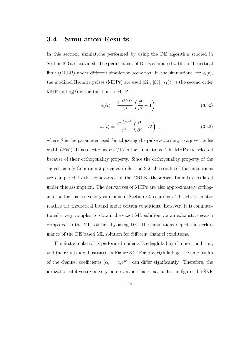
limit (CRLB) under different simulation scenarios. In the simulations, for si(t),

the modified Hermite pulses (MHPs) are used [62], [63]. s1(t) is the second order

MHP and s2(t) is the third order MHP.

s1(t) =e−t

2/4β2

β2

(t2

β2− 1

), (3.32)

s2(t) =e−t

2/4β2

β4

(t3

β2− 3t

), (3.33)

where β is the parameter used for adjusting the pulse according to a given pulse

width (PW ). It is selected as PW/15 in the simulations. The MHPs are selected

because of their orthogonality property. Since the orthogonality property of the

signals satisfy Condition 2 provided in Section 3.2, the results of the simulations

are compared to the square-root of the CRLB (theoretical bound) calculated

under this assumption. The derivatives of MHPs are also approximately orthog-

onal, so the space diversity explained in Section 3.2 is present. The ML estimator

reaches the theoretical bound under certain conditions. However, it is computa-

tionally very complex to obtain the exact ML solution via an exhaustive search

compared to the ML solution by using DE. The simulations depict the perfor-

mance of the DE based ML solution for different channel conditions.

The first simulation is performed under a Rayleigh fading channel condition,

and the results are illustrated in Figure 3.2. For Rayleigh fading, the amplitudes

of the channel coefficients (αi = aiejθi) can differ significantly. Therefore, the

utilization of diversity is very important in this scenario. In the figure, the SNR

45

0 5 10 15 20 25 3010

−1

100

101

102

103

SNR (dB)

RM

SE

(m

.)

MLECRLB

Figure 3.2: The RMSE of the MLE and the square-root of the CRLB for theRayleigh fading channel.

of the system is defined as SNR = 10 log10

(E2σ2

), where E is the energy of one of

the signals transmitted from one antenna (all of the signal energies are set to 1 in

the simulations). The channel coefficients (ai) are Rayleigh distributed random

variables with average power 1 ( E{a2i } = 1 ) and φi’s are distributed as uniform

random variables in the interval [0, 2π). The time-delay τ is generated according

to uniform distribution over the observation interval. The bandwidths of the

signals are B = 1 MHz. The root mean-squared error (RMSE) is calculated over

many channel realizations and this is compared to the square-root of the CRLB.

46

0 5 10 15 20 25 3010

−1

100

101

102

103

SNR (dB)

RM

SE

(m

.)

MLECRLB

Figure 3.3: The RMSE of the MLE and the square-root of the CRLB for theRician fading channel (K = 5).

47

The second simulation investigates the performance of the DE based ML algo-

rithm under Rician fading with K factor 5 [64]. The SNR definition, the average

power of channel coefficients, and the distribution of ai’s and φi’s are the same as

in the previous simulation. Figure 3.3 shows the performance of the algorithm in

this scenario. If the two simulation results are compared, it can be observed that

the presence of strong line-of-sight component in Rician fading causes the esti-

mator to converge the bound (√

CRLB) at lower SNRs compared to the Rayleigh

fading scenario, which does not include a significant line-of-sight component. But,

in both cases, the algorithm converges to the bound at sufficiently high SNRs by

utilizing the space diversity introduced by the transmitter antennas.

48

Chapter 4

TIME-DELAY ESTIMATION IN

COGNITIVE SINGLE-INPUT

MULTIPLE-OUTPUT

SYSTEMS

In this chapter, the time-delay estimation problem in cognitive SIMO systems

is analyzed. In the previous chapters, the same problem is investigated in cog-

nitive systems and MISO systems, which include frequency and space diversity,

respectively. The study in this chapter focuses on facilitation of the combination

of frequency and space diversity in time-delay estimation problem. It should be

kept in mind that the space diversity here takes place as receive diversity.

In the rest of the chapter, the signal model is provided and afterwards the

CRLB for the estimation of time-delay parameter is found. Then, the ML esti-

mator is expressed and two-step approach similar to the one applied in Chapter

49

2 is used to propose an asymptotically optimal solution to the ML estimation.

This solution consists of estimating the signal parameters at each receiver branch

and combining the time-delay estimates at the second step. Various combination

algorithms for combining these time-delay estimates are proposed and the perfor-

mance analyses of them under various scenarios are provided in the simulations.

4.1 Signal Model

In a cognitive SIMO system, there are multiple antennas at the receiver and

a single antenna at the transmitter side because of the SIMO structure. This

structure is depicted in Figure 4.1.

Figure 4.1: SIMO structure.

The transmitted signal utilizes multiple frequency bands. Therefore, the re-

ceived signals at each of the receiver antennas has a dispersed spectrum structure,

50

as shown in Figure 2.1.

The baseband received signal at the kth band of the ith receiver antenna can

be modeled as follows:

rik(t) = αikejwktsk(t− τ) + nik(t) , (4.1)

where i = 1, . . . ,M is the index for the receiver antenna (M is the total number of

receiver antennas) and k = 1, . . . , K is the index for the frequency band (K is the

total number of frequency bands). Here, αik = aik ejφik and wk are the channel

coefficient and the CFO of the corresponding receiver branch, respectively (a

receiver branch is the transmission path from the transmitter to the receiver

for a specific frequency band and a specific antenna). sk(t) is the baseband

representation of the transmitted signal and τ is the time-delay of this signal.

Additionally, nik(t) represents the additive complex white Gaussian noise having

independent components, each with spectral density σ2ik. Also, the noise processes

at different antennas are modeled as independent from each other.

In this signal model, each of the signals, sk(t)’s, are assumed to be narrowband

signals. This facilitates the use of a single channel coefficient to denote the

fading of each signal. Moreover, usage of narrowband signals makes the difference

between time-delays of each received signal so small that the time-delays can be

recognized as equal. Therefore, a single time-delay, τ , is used for each received

signal.

If the separation distances between the receiver antennas are comparable to

the signal wavelength, then the antennas are said to be sufficiently separated

which implies that the channel coefficients can be considered as independent at

different antennas.

51

4.2 CRLB Calculations

The estimation problem investigated in this chapter is the time-delay estima-

tion in a cognitive SIMO system. As mentioned in Section 4.1, as a result of

the narrowband assumption for each frequency band, there is a single unknown

time-delay parameter. Since there is a separate channel coefficient αik for every

receiver branch, there are two unknown parameters (aik and φik) for each branch.

wk’s are the CFOs of the frequency bands, so they are also among the unknown

parameters. To sum up, the unknown signal parameters are given by the vector

θ, which is described below:

θ =[τ a φ w

], (4.2)

where

a =[a11 . . . a1K a21 . . . a2K . . . aM1 . . . aMK

], (4.3)

φ =[φ11 . . . φ1K φ21 . . . φ2K . . . φM1 . . . φMK

], (4.4)

w =[w1 . . . wK

]. (4.5)

If the received signal is observed in the time interval [0, T ], the log-likelihood

function for θ can be obtained from (4.1) as follows [49]:

Λ(θ) = c−M∑i=1

K∑k=1

1

2σ2ik

∫ T

0

∣∣∣rik(t)− αikejwktsk(t− τ)∣∣∣2 dt. (4.6)

By using the log-likelihood expression in (4.6), the FIM is constructed, which

52

can be expressed as

I =

Iττ Iτa Iτφ Iτw

ITτa Iaa Iaφ Iaw

ITτφ ITaφ Iφφ Iφw

ITτw ITaw ITφw Iww

. (4.7)

In order to calculate the FIM, the first derivatives of the log-likelihood function

with respect to the unknown parameters are found and they are provided in

Appendix A.

The submatrices of the FIM are provided below 1 2 3:

Iττ = E

{(∂Λ(θ)

∂τ

)2}

=M∑i=1

K∑k=1

a2ikσ2ik

∫ T

0

|s′k(t− τ)|2 dt =K∑k=1

Ek

M∑i=1

a2ikσ2ik

(4.8)

[Iaa]{ik}{ik} = E

{(∂Λ(θ)

∂aik

)2}

=1

σ2ik

∫ T

0

|sk(t− τ)|2 dt =1

σ2ik

Ek (4.9)

[Iaa]{ik}{jl} = E

{∂Λ(θ)

∂aik

∂Λ(θ)

∂ajl

}= 0 for i6=j or k 6=l (4.10)

[Iφφ]{ik}{ik} = E

{(∂Λ(θ)

∂φik

)2}

=1

σ2ik

∫ T

0

a2ik|sk(t− τ)|2 dt

=a2ikσ2ik

Ek (4.11)

[Iφφ]{ik}{jl} = E

{∂Λ(θ)

∂φik

∂Λ(θ)

∂φjl

}= 0 for i6=j or k 6=l (4.12)

1[X]kl denotes the element of matrix X in row k and column l.2[X]{ik}{jl} denotes the element of matrix X in row (i− 1)K + k and column (j − 1)K + l.3[X]{ik}{l} denotes the element of matrix X in row (i− 1)K + k and column l.

53

[Iww]kk = E

{(∂Λ(θ)

∂wk

)2}

=M∑i=1

a2ikσ2ik

∫ T

0

t2|sk(t− τ)|2 dt (4.13)

[Iww]kl = E

{∂Λ(θ)

∂wk

∂Λ(θ)

∂wl

}= 0 for k 6=l (4.14)

[Iτa]ik = E

{(∂Λ(θ)

∂τ

∂Λ(θ)

∂aik

)}= − 1

σ2ik

∫ T

0

aikR{s′

k(t− τ)s∗k(t− τ)}

=−aikσ2ik

ERk (4.15)

[Iτφ]ik = E

{(∂Λ(θ)

∂τ

∂Λ(θ)

∂φik

)}=−a2ikσ2ik

∫ T

0

I{s′

k(t− τ)s∗k(t− τ)}

=−a2ikσ2ik

EIk (4.16)

[Iτw]k = E

{(∂Λ(θ)

∂τ

∂Λ(θ)

∂wk

)}=

M∑i=1

−a2ikσ2ik

∫ T

0

I{ts

′

k(t− τ)s∗k(t− τ)}

=M∑i=1

−a2ikσ2ik

Gk (4.17)

[Iaφ]{ik}{ik} = E

{(∂Λ(θ)

∂aik

∂Λ(θ)

∂φik

)}= − j

4σ4ik

∫ T

0

−2σ2ikaik|sk(t− τ)|2 + 2σ2

ikaik|sk(t− τ)|2 dt = 0 (4.18)

[Iaφ]{ik}{jl} = E

{(∂Λ(θ)

∂aik

∂Λ(θ)

∂φjl

)}= 0 for i 6=j or k 6=l (4.19)

[Iaw]{ik}{k} = E

{(∂Λ(θ)

∂aik

∂Λ(θ)

∂wk

)}= − j

4σ4ik

∫ T

0

−t2σ2ikaik|sk(t− τ)|2 + t2σ2

ikaik|sk(t− τ)|2 dt = 0

(4.20)

54

[Iaw]{ik}{l} = E

{(∂Λ(θ)

∂aik

∂Λ(θ)

∂wl

)}= 0 for k 6=l (4.21)

[Iφw]{ik}{l} = E

{(∂Λ(θ)

∂φik

∂Λ(θ)

∂wl

)}= 0 for k 6=l (4.22)

[Iφw]{ik}{k} = E

{(∂Λ(θ)

∂φik

∂Λ(θ)

∂wk

)}= − 1

4σ4ik

∫ T

0

−2σ2ikta

2ik|sk(t− τ)|2 − 2σ2

iktaik|sk(t− τ)|2 dt (4.23)

=a2ikσ2ik

∫ T

0

t|sk(t− τ)|2 dt =a2ikσ2ik

Fk

The theoretical lower bound on the variance of an unbiased estimator is the

CRLB. The problem investigated in this study is the time-delay estimation in a

cognitive SIMO system; hence, the CRLB for the time-delay parameter must be

found. The CRLB can be obtained from the inverse of the FIM. The CRLB for

the time-delay parameter is the first element of the inverse of the FIM, which is

[I−1]11.

Before finding the CRLB, it is useful to observe that for any linear modulation

in the form of sk(t) =∑

n dk,npk(t− nTk), EIk = 0 and Gk = 0 (cf. Proposition 1

in [43]).

If the FIM is partitioned in the following form,

I =

A B

BT D

, (4.24)

where

A =[Iττ

], B =

[Iτa Iτφ Iτw

], D =

Iaa 0 0

0 Iφφ Iφw

0 ITφw Iww

, (4.25)

55

then the CRLB, which is the first element of the inverse of the FIM, can be found

in the following way:[I−1]11

= (A−BD−1BT)−1

=(Iττ − IτaI

−1aa ITτa

)−1=

1∑Kk=1 Ek

∑Mi=1

a2ikσ2ik− a2ik

σ4ik

(ERk )2

σ2ik

Ek

=1∑K

k=1

∑Mi=1

a2ikσ2ik

(Ek −

(ERk )2

Ek

) (4.26)

Furthermore, if the linear modulation of the form sk(t) =∑

n dk,npk(t− nTk)

is with |dk,n| = |dk| and pk(0) = pk(Ti), then ER = 0 (cf. Proposition 2 in [43]).

Finally, the CRLB becomes[I−1]1x1

=1∑K

k=1

∑Mi=1

a2ikσ2ikEk. (4.27)

4.3 CRLB Calculations for Single Band and Sin-

gle Antenna Systems

For a receiver branch, which means the channel between the transmitter and a

receiver antenna for a single frequency band, the unknown parameter vector, θik,

can be described as

θik =[τik aik φik wik

], (4.28)

where the definitions of the parameters are the same as in Section 4.1.

The model for the baseband received signal is provided in (4.1). In our two-

step approach for time-delay estimation, the unknown parameters for the received

56

signal is estimated separately at each branch. Therefore, the baseband received

signal model can be modified to be as follows:

rik(t) = αikejwiktsk(t− τik) + nik(t) , (4.29)

with the same definitions for the received and transmitted signals, and the noise

process as in Section 4.1.

From (4.29), the log-likelihood function for θik can be expressed as follows:

Λ(θik) = c− 1

2σ2ik

∫ T

0

∣∣∣rik(t)− αikejwiktsk(t− τik)∣∣∣2 dt, (4.30)

assuming that the received signal is observed in the time interval [0, T ]. Here, c

is a constant that is independent of θik.

The FIM for the time-delay estimation problem in a receiver branch, which

is obtained from (4.30), is as follows:

I =

Iττ Iτa Iτφ Iτw

ITτa Iaa Iaφ Iaw

ITτφ ITaφ Iφφ Iφw

ITτw ITaw ITφw Iww

. (4.31)

In order to calculate the FIM, the first derivatives of the log-likelihood function

with respect to the unknown parameters are found and they are provided in

Appendix B.

The submatrices of the FIM are provided below:

Iττ = E

{(∂Λ(θ)

∂τik

)2}

=1

σ4ik

∫ T

0

a2ikσ2ik|s

′

k(t− τik)|2 dt

=a2ikσ2ik

Ek (4.32)

57

Iaa = E

{(∂Λ(θ)

∂aik

)2}

=1

σ4ik

∫ T

0

|sk(t− τik)|2σ2ik dt

=1

σ2ik

Ek (4.33)

Iφφ = E

{(∂Λ(θ)

∂φik

)2}

=1

σ4ik

∫ T

0

a2ik|sk(t− τik)|2σ2ik dt

=a2ikσ2ik

Ek (4.34)

Iww = E

{(∂Λ(θ)

∂wik

)2}

=1

σ4ik

∫ T

0

t2a2ik|sk(t− τik)|2σ2ik dt

=a2ikσ2ik

∫ T

0

t2|sk(t− τik)|2 dt (4.35)

Iτa = E

{(∂Λ(θ)

∂τik

∂Λ(θ)

∂aik

)}= − 1

σ4ik

∫ T

0

σ2ikaikR

{s′

k(t− τik)s∗k(t− τik)}

=−aikσ2ik

ERk (4.36)

Iτφ = E

{(∂Λ(θ)

∂τik

∂Λ(θ)

∂φik

)}=−a2ikσ2ik

∫ T

0

I{s′

k(t− τik)s∗k(t− τik)}

=−a2ikσ2ik

EIk (4.37)

Iτw = E

{(∂Λ(θ)

∂τik

∂Λ(θ)

∂wik

)}=−a2ikσ2ik

∫ T

0

I{ts

′

k(t− τik)s∗k(t− τik)}

=−a2ikσ2ik

Gk (4.38)

Iaφ = E

{(∂Λ(θ)

∂aik

∂Λ(θ)

∂φik

)}= − j

4σ4ik

∫ T

0

−2σ2ikaik|sk(t− τik)|2 + 2σ2

ikaik|sk(t− τik)|2 dt = 0 (4.39)

58

Iaw = E

{(∂Λ(θ)

∂aik

∂Λ(θ)

∂wik

)}= − j

4σ4ik

∫ T

0

−t2σ2ikaik|sk(t− τik)|2 + t2σ2

ikaik|sk(t− τik)|2 dt = 0 (4.40)

Iφw = E

{(∂Λ(θ)

∂φik

∂Λ(θ)

∂wik

)}= − 1

4σ4ik

∫ T

0

−2σ2ikta

2ik|sk(t− τik)|2 − 2σ2

iktaik|sk(t− τik)|2 dt

=a2ikσ2ik

∫ T

0

t|sk(t− τik)|2 dt =a2ikσ2ik

Fk (4.41)

The FIM can be written as I =

A B

BT D

where A =

Iττ Iτa

ITτa Iaa

, B =

Iτφ Iτw

0 0

, and D =

Iφφ Iφw

ITφw Iww

. The first 2-by-2 block of I can be calculated

as[I−1]2×2

= (A−BD−1BT)−1.

If Ek = 0, then Iτa = 0, and Iτφ = 0. If also Iτw = 0 is satisfied, then

[I−1]2×2

=

σ2ik

a2ikEk0

0σ2ik

Ek

(4.42)

becomes valid.

This result leads us to the following lemma on the delay and channel amplitude

estimates at high SNRs.

Lemma 2: Consider any linear modulation of the form sk(t) =∑

n dk,npk(t−

nTk), where dk,n denotes the complex data for the nth symbol of signal k, and pk(t)

represents a pulse with duration Tk. Assume that∫∞−∞ s

′k(t−τ)s∗k(t−τ)dt = 0 for

k = 1, . . . , K. Then, for the signal model in (4.1), the delay estimate in (4.48)

59

and the channel amplitude estimate in (4.49) can be modeled, at high SNR, as

τik = τ + νik , (4.43)

aik = aik + ηik , (4.44)

for k = 1, . . . , K and i = 1, . . . ,M , where νik and ηik are independent zero mean

Gaussian random variables with variances σ2ik/(Ek a

2ik) and σ2

ik/Ek, respectively.

In addition, νik and νjl (ηik and ηjl) are independent for i 6= j and k 6= l.

4.4 Two-Step Time-Delay Estimation

The optimal solution for the time-delay estimation is the parameter vector that

maximizes the log-likelihood function given in (4.6). This solution, which is the

ML estimate, can be expressed as follows:

θ = arg maxθ

{c−

M∑i=1

K∑k=1

1

2σ2ik

∫ T

0

∣∣∣rik(t)− αikejwktsk(t− τ)∣∣∣2 dt} . (4.45)

This ML estimate includes an optimization over 2MK + K + 1 variables,

which has huge computational complexity. To avoid such a complex method, an

alternative two-step solution is proposed to this problem.

In the first step, using the received signal, the ML estimate for the time-delay

parameter is found for every receiver branch (If there are M receiver antennas

and K frequency branches, then there are M×K branches.). The weighted com-

bination of the time-delay estimates obtained from each branch is the second step

of the time-delay estimation process. The weights used in this step determines

the complexity and accuracy of the estimator. The two-step approach is depicted

in Figure 4.2.

60

Figure 4.2: Illustration of the two-step time-delay estimation algorithm for acognitive SIMO system.

61

4.4.1 First Step: Maximum Likelihood Estimation at Each

Branch

The unknown parameters at each branch are denoted by vector θik, as mentioned

in (4.28). The ML estimate for these unknown parameters is the set of parameter

values that maximize the log-likelihood function in (4.30); that is,

θik = arg maxθik

{c− 1

2σ2ik

∫ T

0

∣∣∣rik(t)− αikejwiktsk(t− τik)∣∣∣2 dt} , (4.46)

which is equivalent to

θik = arg minθik

∫ T

0

∣∣∣rik(t)− αikejwiktsk(t− τik)∣∣∣2 dt . (4.47)

At each branch, the unknown parameters are estimated separately and they

are denoted by the unknown parameter vector θik =[τik aik φik wik

]. The

expression in (4.47) is separable into two parts, so is the ML estimation process.

Therefore, the optimization problem in (4.47) can be performed in two steps as

follows:[τik φik ωik

]= arg max

τik,ωik,φik

∣∣∣∣∫ T

0

R{rik(t) e−j(ωikt+φik)s∗ik(t− τik)

}dt

∣∣∣∣ (4.48)

and

aik =1

Eik

∫ T

0

R{rik(t) e−j(ωikt+φik)s∗ik(t− τik)

}dt . (4.49)

In this way, the optimization process over 2MK + K + 1 variables that the

ML estimation in (4.45) requires is avoided and this process in handled by MK

optimizations each of which are over 3 variables.

If it is assumed that the CFOs (wik’s) are zero, which means that the carrier

frequencies are known, then the wik’s in (4.48) and (4.49) will be omitted and

the equations will become as follows:

62

[τik φik

]= arg max

τik,φik

∣∣∣∣∫ T

0

R{rik(t) e−jφiks∗ik(t− τik)

}dt

∣∣∣∣ (4.50)

and

aik =1

Eik

∫ T

0

R{rik(t) e−jφiks∗ik(t− τik)

}dt . (4.51)

4.4.2 Second Step: Combining Time-Delay Estimates from

Different Branches

1. Optimal Combining: In this combining method, the time-delay estimates

obtained from each receiver branch are combined. This is performed by

finding the weighted average of MK time-delay estimates. The weight

determined for each branch is expressed as

βik =a2ikEikσ2ik

. (4.52)

Using these weights, the combining is performed as follows:

τ =

∑Mi=1

∑Kk=1 βikτik∑M

i=1

∑Kk=1 βik

. (4.53)

By a similar discussion to the one provided in Section 2.3.2 about the effec-

tive bandwidth component in the weights used in optimal combining, the

weights used here also means to combine the time-delay estimates of differ-

ent branches in proportion to the multiplication of the SNR estimate and

the effective bandwidth of that branch, which means that the optimal com-

bining considers both the SNR and the effective bandwidth of the branches

while calculating the weighted average of time-delay estimates.

63

2. SNR Combining: In this combining method, the weights assigned to each

time-delay estimate obtained from the branches are as follows:

µik =a2ikEikσ2ik

. (4.54)

These weights are used for combining the estimates as

τ =

∑Mi=1

∑Kk=1 µikτik∑M

i=1

∑Kk=1 µik

. (4.55)

The difference between this estimator and the optimal combining estimator

is that SNR combining only weights the branches according to their SNR

values, whereas optimal combining considers both the SNR and effective

bandwidth values. SNR combining omits the effective bandwidth term in

the weights.

3. Selection Combining 1: In the previous two combining methods, the weighted

average of the estimates are used as the final time-delay estimate. In selec-

tion combining, the best branch is used as the final time-delay estimate.

In selection combining 1, the definition of the best branch is in terms of the

weights that are used in the optimal combining method. The time-delay

of the branch that has the maximum βik is selected as the final time-delay

estimate; that is,

τ = τjl , (4.56)

with

{j, l} = arg maxi∈{1,...,M}, k∈{1,...,K}

{βik}

= arg maxi∈{1,...,M}, k∈{1,...,K}

{a2ikEikσ2ik

}, (4.57)

64

where j and l are the i and k indices of the branch that have the maximum

βik.

4. Selection Combining 2: In selection combining 2, the best branch is se-

lected by using the SNR values of the receiver branches. The SNR value

of each branch is as it is defined in the “SNR combining” method, that is

µik = a2ikEik/σ2ik. Hence, the selection combining method 2 is performed as

follows:

τ = τjl , (4.58)

with

{j, l} = arg maxi∈{1,...,M}, k∈{1,...,K}

{µik}

= arg maxi∈{1,...,M}, k∈{1,...,K}

{a2ikEikσ2ik

}. (4.59)

5. Equal Combining: In this combining method, the time-delay estimates from

different branches are combined regardless of their “importance”. That

is, in equal combining, all of the time-delay estimates are assigned equal

weights

τ =1

MK

M∑i=1

K∑k=1

τik . (4.60)

4.5 Optimality of the Two-Step Estimator

The rule for the two-step estimator that employs optimal combining is

τ =

∑Mi=1

∑Kk=1 βikτik∑M

i=1

∑Kk=1 βik

, (4.61)

65

where

βik =a2ikEkσ2ik

, (4.62)

as mentioned before.

It can be shown that

E {τ |aik...} =

∑Mi=1

∑Kk=1 βikE{τik|aik...}∑Mi=1

∑Kk=1 βik

=

∑Mi=1

∑Kk=1 βikE{τik|aik}∑Mi=1

∑Kk=1 βik

(4.63)

= τ = E{τ} (4.64)

Hence, the estimator is unbiased. (The equality of the above expression to τ

results from Lemma 2)

On the other hand, the conditional variance can be expressed as

Var {τ |aik...} =

∑Mi=1

∑Kk=1 β

2ikVar{τik|aik...}(∑M

i=1

∑Kk=1 βik

)2 . (4.65)

From the same lemma, Var {τ |aik...} = Var {τ |aik} =σ2ik

a2ikEk. Then

Var {τ |aik...} =

∑Mi=1

∑Kk=1

a4ikE2k

σ4ik

σ2ik

a2ikEk(∑Mi=1

∑Kk=1

a2ikEk

σ2ik

)2 . (4.66)

According to the lemma; at high SNRs, aik is distributed as a Gaussian random

variable with mean aik and variance σ2ik/Ek.

Var {τ |aik...} ≈1∑M

i=1

∑Kk=1

a2ikσ2ikEk

, (4.67)

which is equal to the CRLB. Hence, the estimator is approximately optimal at

high SNRs.

Optimality of the estimator can also be proved when the other combining

techniques are used. An example of such proof for SNR combining can be carried

out similar to the proof in Section 2.4.

66

4.6 Simulation Results

Simulations are performed in order to compare the performance of the various

combining methods proposed in Section 4.4. The performance evaluation of these

methods is carried out by comparing them with each other and with the theoret-

ical bound, the CRLB.

In the simulations, the signal at each branch, sk(t) in (4.1), is modeled by the

Gaussian doublet which can be expressed as follows:

sk(t) = Ak

(1− 4π(t− 1.25 ζk)

2

ζ2k

)e−2π(t−1.25ζk)

2/ζ2k , (4.68)

where Ak is the parameter that adjusts the energy of the pulse. In the following

simulations, the pulses are adjusted to have unit-energy. ζk is the parameter that

adjusts the pulse width which can be approximately expressed as ζk ≈ 1/(2.5Bk)

in terms of the bandwidth Bk of the signal sk(t) [25].

For all the simulations, the time-delay, τ , is uniformly distributed over the

observation interval. The distribution of φik is also the same for all the simula-

tions, which is uniform distribution in the interval [0, 2π). For different branches,

the spectral density of the noise process is assumed to be the same. Additionally,

the definition of the SNR is the same for all the simulation scenarios, which is

SNR = 10 log10

(∑Mi=1

∑Kk=1 Eik

2σ2ik

).

In Figure 4.3, the first simulation result is presented. It depicts the per-

formance of the estimators in terms of the RMSE as the SNR increases. The

distribution of the magnitude of each channel coefficient, aik, is assumed to be

Rayleigh distributed with an average power of 1, i.e. E{|α2ik|} = E{a2ik} = 1.

There are 2 antennas (M = 2) and 3 spectrum bands (K = 3) with different

bandwidths, i.e. 100 kHz, 200 kHz, and 400 kHz.

67

0 5 10 15 2010

−8

10−7

10−6

10−5

SNR (dB)

RM

SE

(se

c.)

Optimal combiningSNR combiningEqual combiningSelection combining 1Selection combining 2Theoretical limit

Figure 4.3: The performances of the estimators, RMSE vs. SNR, and the theo-retical limit (CRLB). There are 2 receive antennas, 3 dispersed bands with 100kHz, 200 kHz, and 400 kHz bandwidths under Rayleigh fading condition.

As observed from Figure 4.3, in this simulation scenario, the best perfor-

mance is achieved by the optimal combining estimator. Selection combining 1

is the second best after optimal combining. SNR combining has worse perfor-

mance than optimal combining and selection combining 1. Selection combining

2, which selects the best branch in terms of the SNR values of the branches, has

worse performance than SNR combining, which takes the weighted average of the

time-delays by using their SNRs. Equal combining has the worst performance

among all of the estimators, since it takes the average of the time-delay estimates

68

regardless of the “importances” of the branches.

0 5 10 15 2010

−8

10−7

10−6

10−5

SNR (dB)

RM

SE

(se

c.)

Optimal combiningSNR combiningEqual combiningSelection combining 1Selection combining 2Theoretical limit

Figure 4.4: The performances of the estimators, RMSE vs. SNR, and the theo-retical limit (CRLB). There are 2 receive antennas, 3 dispersed bands each with100 kHz bandwidth under Rayleigh fading condition.

Figure 4.4 provides the performance of the estimators under the same sce-

nario as in Figure 4.3, except for the bandwidths of the frequency bands. The

bandwidths are the same for all bands, which is 100 kHz for each band.

As mentioned before, the optimal combining algorithm uses βik = a2ikEik/σ2ik

and the SNR combining uses µik = a2ikEik/σ2ik as the weights for each branch. In

this case, since the bandwidths for all the bands are the same, the energies of the

signals at different branches will be equal to each other. Similarly, the energies of

69

the signal derivatives will also be equal at all the branches. Therefore, for both

optimal combining and SNR combining, the time-delays of different branches

will be combined effectively by using a2ik/σ2ik, which means the omission of Eik

and Eik from βik and µik, respectively. This leads to the same final time-delay

estimates for SNR and optimal combining methods, as seen in Figure 4.4. Since

selection combining methods are based on selecting the time-delays of the best

branches by using the same criteria as the optimal and SNR combining, they also

give the same final estimate. The best performance is achieved by optimal/SNR

combining pair, as expected. The selection combining is worse than this pair.

Equal combining is the worst, as before.

The results of the simulations which test the estimators’ RMSE performance

as the number of spectrum bands increases are depicted in Figure 4.5. The

number of antennas is two (M = 2). The bandwidths of the signals at different

bands are all equal to 100 kHz. The spectral density of the noise processes is

the same at each branch, as mentioned before. The distributions of the channel

parameters are selected to be the same as in the previous simulations.

Since the bandwidths of the frequency bands are the same, the SNR combining

and the optimal combining methods show the same performance, like the selection

combining methods do. As before, the estimators are ranked in following order

depending on their performances: Optimal combining, selection combining, and

equal combining. It is notable that when the number of bands reaches 5, the

return of the selection combining becomes negligible as the number of bands

continues increasing. Another point is that the return of the equal combining

increases as the number of bands increases.

The next simulation scenario has 3 frequency bands with 100 kHz, 200 kHz,

70

0 5 10 15 2010

−8

10−7

10−6

10−5

Number of Bands

RM

SE

(se

c.)

Optimal combiningSNR combiningEqual combiningSelection combining 1Selection combining 2Theoretical limit

Figure 4.5: The performances of the estimators, RMSE vs. number of bands,and the theoretical limit (CRLB). There are 2 receive antennas under Rayleighfading condition.

and 400 kHz bandwidths. In this case, the performance analysis is carried out

as the number of receive antennas is increased. The other simulation parameters

are the same as in the previous simulations. In Figure 4.6, the results of this

simulation can be observed.

The best performance result again belongs to optimal combining. The SNR

combining and selection combining 1 methods are so close to each other, which

come after optimal combining. Selection combining 2 performs worse than these

estimators. The performance of equal combining is way worse than the others

71

1 1.5 2 2.5 3 3.5 4 4.5 510

−8

10−7

10−6

10−5

Number of Antennas

RM

SE

(se

c.)

Optimal combiningSNR combiningEqual combiningSelection combining 1Selection combining 2Theoretical limit

Figure 4.6: The performances of the estimators, RMSE vs. number of antennas,and the theoretical limit (CRLB). There are 3 dispersed bands with 100 kHz, 200kHz, and 400 kHz bandwidths under Rayleigh fading condition.

but it comes closer as the number of bands increases.

Figure 4.7 illustrates the results of a similar simulation scenario as the previous

one, the only difference being the same bandwidth usage for all frequency bands;

i.e., 100 kHz instead of using different bandwidths.

Similar to the simulation results depicted in Figure 4.6, the optimal combin-

ing is the best, followed by the selection combining and the equal combining.

Moreover, as in the simulation results in Figure 4.4, the optimal combining has

the same performance as the SNR combining, and selection combining methods

72

1 1.5 2 2.5 3 3.5 4 4.5 510

−8

10−7

10−6

10−5

Number of Antennas

RM

SE

(se

c.)

Optimal combiningSNR combiningEqual combiningSelection combining 1Selection combining 2Theoretical limit

Figure 4.7: The performances of the estimators, RMSE vs. number of antennas,and the theoretical limit (CRLB). There are 3 dispersed bands each with 100 kHzbandwidth under Rayleigh fading condition.

are also the same in terms of the RMSE performance.

In the following set of simulations, the distribution of the magnitude of the

channel coefficients is selected as Rician distribution with an average power of

1, i.e. E{|a2ik|} = 1. The K factor of Rician distribution is selected as 5. Ri-

cian fading assumption replaces the Rayleigh fading assumption in the first 5

simulations. The simulation pairs that use the same simulation scenarios other

than the Rician-Rayleigh fading replacement are as follows: Figure 4.3-Figure

4.8, Figure 4.4-Figure 4.9, Figure 4.5-Figure 4.10, Figure 4.6-Figure 4.11, and

73

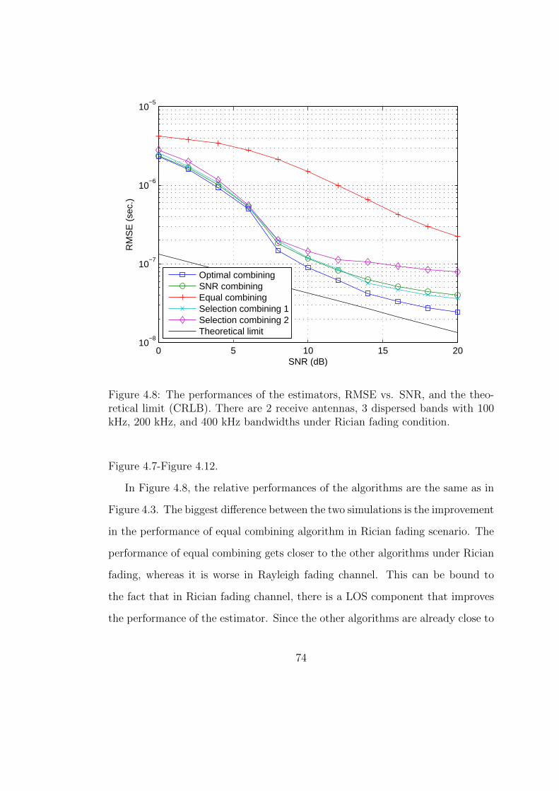
0 5 10 15 2010

−8

10−7

10−6

10−5

SNR (dB)

RM

SE

(se

c.)

Optimal combiningSNR combiningEqual combiningSelection combining 1Selection combining 2Theoretical limit

Figure 4.8: The performances of the estimators, RMSE vs. SNR, and the theo-retical limit (CRLB). There are 2 receive antennas, 3 dispersed bands with 100kHz, 200 kHz, and 400 kHz bandwidths under Rician fading condition.

Figure 4.7-Figure 4.12.

In Figure 4.8, the relative performances of the algorithms are the same as in

Figure 4.3. The biggest difference between the two simulations is the improvement

in the performance of equal combining algorithm in Rician fading scenario. The

performance of equal combining gets closer to the other algorithms under Rician

fading, whereas it is worse in Rayleigh fading channel. This can be bound to

the fact that in Rician fading channel, there is a LOS component that improves

the performance of the estimator. Since the other algorithms are already close to

74

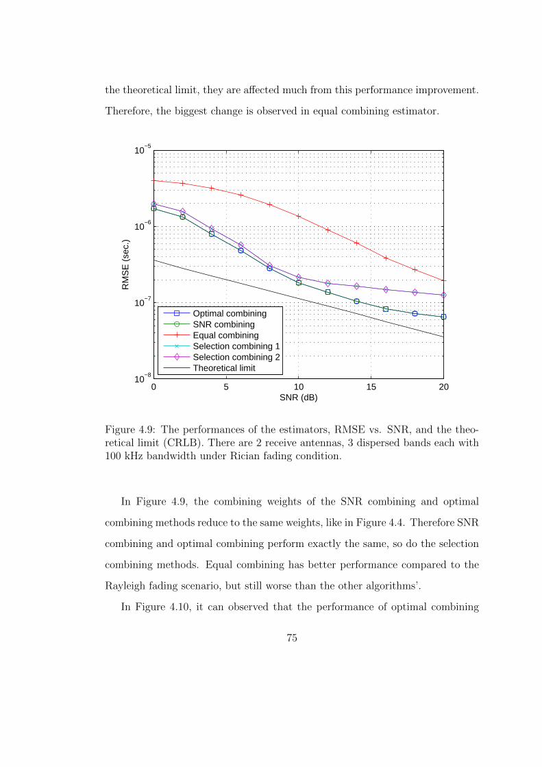
the theoretical limit, they are affected much from this performance improvement.

Therefore, the biggest change is observed in equal combining estimator.

0 5 10 15 2010

−8

10−7

10−6

10−5

SNR (dB)

RM

SE

(se

c.)

Optimal combiningSNR combiningEqual combiningSelection combining 1Selection combining 2Theoretical limit

Figure 4.9: The performances of the estimators, RMSE vs. SNR, and the theo-retical limit (CRLB). There are 2 receive antennas, 3 dispersed bands each with100 kHz bandwidth under Rician fading condition.

In Figure 4.9, the combining weights of the SNR combining and optimal

combining methods reduce to the same weights, like in Figure 4.4. Therefore SNR

combining and optimal combining perform exactly the same, so do the selection

combining methods. Equal combining has better performance compared to the

Rayleigh fading scenario, but still worse than the other algorithms’.

In Figure 4.10, it can observed that the performance of optimal combining

75

0 5 10 15 2010

−8

10−7

10−6

10−5

Number of Bands

RM

SE

(se

c.)

Optimal combiningSNR combiningEqual combiningSelection combining 1Selection combining 2Theoretical limit

Figure 4.10: The performances of the estimators, RMSE vs. number of bands,and the theoretical limit (CRLB). There are 2 receive antennas under Ricianfading condition.

stays close to the CRLB as the number of bands increases, whereas the selection

combining methods exhibit a diminishing return, that is after 5 bands there is

almost no improvement. The equal combining performs the worst of all. There is

no significant difference in performance between Rayleigh fading (cf. Figure 4.5)

and Rician fading versions (cf. Figure 4.10).

In Figure 4.11, it can be observed that as the number of antennas increases,

the performances of the algorithms increase. Here, again, the best performance

belongs to the optimal combining, which becomes closer to the CRLB as the

76

1 1.5 2 2.5 3 3.5 4 4.5 510

−8

10−7

10−6

10−5

Number of Antennas

RM

SE

(se

c.)

Optimal combiningSNR combiningEqual combiningSelection combining 1Selection combining 2Theoretical limit

Figure 4.11: The performances of the estimators, RMSE vs. number of antennas,and the theoretical limit (CRLB). There are 3 dispersed bands with 100 kHz, 200kHz, and 400 kHz bandwidths under Rician fading condition.

number of antennas increases. Selection combining 1 and SNR combining perform

almost the same. Similar to the previous simulation, under Rayleigh fading and

Rician fading assumptions, the algorithms perform almost the same.

In Figure 4.12, the performances of the algorithms are similar to the pre-

vious simulation (cf. Figure 4.11), the only difference being the same weight

usage in SNR and optimal combining algorithms, and so in selection combining

algorithms.

77

1 1.5 2 2.5 3 3.5 4 4.5 510

−8

10−7

10−6

10−5

Number of Antennas

RM

SE

(se

c.)

Optimal combiningSNR combiningEqual combiningSelection combining 1Selection combining 2Theoretical limit

Figure 4.12: The performances of the estimators, RMSE vs. number of antennas,and the theoretical limit (CRLB). There are 3 dispersed bands each with 100 kHzbandwidth under Rician fading condition.

78

Chapter 5

Conclusions

In this thesis, the time-delay estimation problems in cognitive radio systems,

MISO systems, and cognitive SIMO systems have been studied.

In time-delay estimation for dispersed spectrum cognitive radio systems, after

the investigation of the ML estimator and the CRLBs, a two-step approach has

been proposed to obtain accurate time-delay estimates with reasonable compu-

tational complexity. In the first step of the proposed approach, an ML estimator

is used at each branch of the receiver in order to estimate the unknown param-

eters of the received signal at that branch. Then, in the second step, a number

of diversity combining approaches have been studied. In the optimal combining

technique, both the SNRs and the bandwidths of the signals at different branches

are considered to obtain the time-delay estimate, whereas the SNR combining

technique obtains the time-delay estimate according to the estimated SNR val-

ues only. In addition, two selection combining techniques, as well as the equal

combining technique, have been investigated. It has been shown that the opti-

mal combining technique can approximate the CRLB at high SNRs, whereas the

79

equal combining technique has the worst performance since it does not make use

of any information about signal bandwidths and/or the SNRs. Simulation results

have been presented to verify the theoretical analysis.

In the time-delay estimation for MISO systems study, the expression for the

theoretical limit (CRLB) has been found. The ML estimator achieves the CRLB

under certain conditions; however, it can have very high computational com-

plexity. To avoid this, a genetic global optimization algorithm has been used to

obtain the ML estimate with lower computational complexity. It has been ob-

served that DE can find the ML estimate much more rapidly than the exhaustive

search method, and that the parameters of DE are crucial in terms of obtaining

the optimum point that maximizes the log-likelihood function. The optimum

parameter values have been selected for DE and applied in the algorithm. In

addition, this study has emphasized the importance of space diversity for the

time-delay estimation problem in MISO systems. It has been stated that the

transmit diversity can be utilized by using signals with orthogonal derivatives.

Finally, the performance of DE has been tested under various channel conditions.

It has been observed that the DE based ML algorithm converges to the CRLB

at lower SNRs in the Rician fading channel than in the Rayleigh fading one.

However, in both of the scenarios, the algorithm reaches the CRLB at sufficiently

high SNRs by utilizing the transmit diversity, with much lower computational

complexity than the ML estimator via an exhaustive search.

In the last study of this thesis, which is the analysis of the time-delay estima-

tion problem in cognitive SIMO systems, the approach is similar to the one in the

estimation problem in cognitive radio systems. The CRLB has been found and

the two-step time-delay estimation has been proposed. The performance analysis

80

of the algorithms applied in the second step of this two-step approach has been

carried out. It has been observed in the simulations that optimal estimator has

the best performance among all estimators. The effective bandwidth property

of the signals has not been taken into account in SNR combining algorithm, al-

though it has been done so in optimal combining. Therefore, SNR combining

performs a little bit worse than the optimal combining. Selection combining al-

gorithms select the time-delay estimate of the “best” branch, which trade off

simplicity with performance. Equal combining is the simplest and the worst of

all. Changing the fading assumption from Rayleigh fading to Rician fading is

shown to significantly improve the estimator performance of equal combining in

some simulations.

Finally, joint analysis of the time-delay estimation problems of MISO sys-

tems and cognitive SIMO systems leads to the analysis of the same problem in

cognitive MIMO systems. This follows from the fact that a MIMO system can

be perceived as multiple MISO systems connected to each receiver antenna of a

SIMO system. The inclusion of dispersed spectrum structure to a MIMO system

results in a cognitive MIMO system, which can be handled in analysis belonging

to the cognitive SIMO systems. Therefore, the most general scenario, the time-

delay estimation problem in a system with space diversity both at the receiver

and the transmitter, and with frequency diversity, is developed and analyzed in

the framework in this thesis.

81

Appendix A

Assuming the received signal is observed in the time interval [0, T ], from Eq.

(4.1), the log-likelihood function for θ can be found as follows [49]:

Λ(θ) =c−M∑i=1

K∑k=1

1

2σ2ik

∫ T

0

∣∣∣rik(t)− αikejwktsk(t− τ)∣∣∣2 dt

=c−M∑i=1

K∑k=1

1

2σ2ik

∫ T

0

{rik(t)− aikejφik+jwktsk(t− τ)

}{r∗ik(t)− aike−jφik−jwkts∗k(t− τ)

}dt

=c−M∑i=1

K∑k=1

1

2σ2ik

∫ T

0

|rik(t)|2 − rik(t)aike−jφik−jwkts∗k(t− τ) (A.1)

− r∗ik(t)aikejφik+jwktsk(t− τ) + a2ik|sk(t− τ)|2 dt

The first derivatives of the log-likelihood function are provided in equations

82

(A.2), (A.3), (A.4), and (A.5).

∂Λ(θ)

∂τ=−

M∑i=1

K∑k=1

1

2σ2ik

∫ T

0

rik(t)aike−jφik−jwkts

′∗k (t− τ)

+ r∗ik(t)aikejφik+jwkts

′

k(t− τ)

− a2iksk(t− τ)s′∗k (t− τ)− a2iks

′

k(t− τ)s∗k(t− τ) dt

=−M∑i=1

K∑k=1

1

2σ2ik

∫ T

0

α∗ik

(rik(t)− αikejwktsk(t− τ)

)s′∗k (t− τ)e−jwkt

+ αik

(r∗ik(t)− α∗ike−jwkts∗k(t− τ)

)s′

k(t− τ)ejwkt dt

=−M∑i=1

K∑k=1

1

2σ2ik

∫ T

0

α∗iknik(t)e−jwkts

′∗k (t− τ) (A.2)

+ αikn∗ik(t)e

jwkts′

k(t− τ) dt

∂Λ(θ)

∂aik=

1

2σ2ik

∫ T

0

rik(t)e−jφik−jwkts∗k(t− τ)

+ r∗ik(t)ejφik+jwktsk(t− τ)− 2aik|sk(t− τ)|2 dt

=1

2σ2ik

∫ T

0

s∗k(t− τ)e−jφik−jwkt(rik(t)− αikejwktsk(t− τ)

)+ sk(t− τ)ejφik+jwkt

(r∗ik(t)− α∗ike−jwkts∗k(t− τ)

)dt

=1

2σ2ik

∫ T

0

s∗k(t− τ)e−jφik−jwktnik(t) + sk(t− τ)ejφik+jwktn∗ik(t) dt (A.3)

∂Λ(θ)

∂φik=− 1

2σ2ik

∫ T

0

jrik(t)aike−jφik−jwkts∗k(t− τ)

− jr∗ik(t)aikejφik+jwktsk(t− τ) dt

=−j2σ2

ik

∫ T

0

(αike

jwktsk(t− τ) + nik(t))aike

−jφik−jwkts∗k(t− τ)

−(α∗ike

−jwkts∗k(t− τ) + n∗ik(t))aike

jφik+jwktsk(t− τ) dt

=−j2σ2

ik

∫ T

0

nik(t)α∗ike−jwkts∗k(t− τ)− n∗ik(t)αikejwktsk(t− τ) dt (A.4)

83

∂Λ(θ)

∂wk=−

M∑i=1

1

2σ2ik

∫ T

0

jtrik(t)aike−jφik−jwkts∗k(t− τ)

− jtr∗ik(t)aikejφik+jwktsk(t− τ) dt

=−M∑i=1

j

2σ2ik

∫ T

0

tnik(t)α∗ike−jwkts∗k(t− τ)− tn∗ik(t)αikejwktsk(t− τ) dt

(A.5)

84

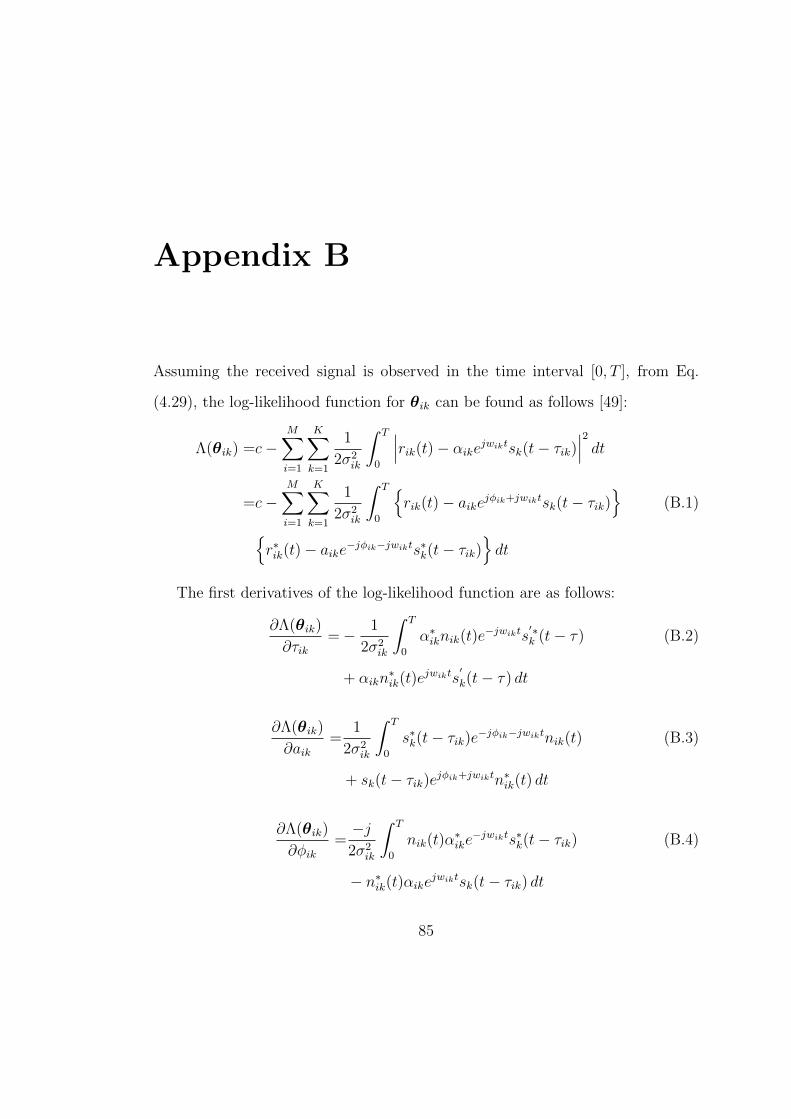
Appendix B

Assuming the received signal is observed in the time interval [0, T ], from Eq.

(4.29), the log-likelihood function for θik can be found as follows [49]:

Λ(θik) =c−M∑i=1

K∑k=1

1

2σ2ik

∫ T

0

∣∣∣rik(t)− αikejwiktsk(t− τik)∣∣∣2 dt

=c−M∑i=1

K∑k=1

1

2σ2ik

∫ T

0

{rik(t)− aikejφik+jwiktsk(t− τik)

}(B.1){

r∗ik(t)− aike−jφik−jwikts∗k(t− τik)}dt

The first derivatives of the log-likelihood function are as follows:

∂Λ(θik)

∂τik=− 1

2σ2ik

∫ T

0

α∗iknik(t)e−jwikts

′∗k (t− τ) (B.2)

+ αikn∗ik(t)e

jwikts′

k(t− τ) dt

∂Λ(θik)

∂aik=

1

2σ2ik

∫ T

0

s∗k(t− τik)e−jφik−jwiktnik(t) (B.3)

+ sk(t− τik)ejφik+jwiktn∗ik(t) dt

∂Λ(θik)

∂φik=−j2σ2

ik

∫ T

0

nik(t)α∗ike−jwikts∗k(t− τik) (B.4)

− n∗ik(t)αikejwiktsk(t− τik) dt

85

∂Λ(θik)

∂wik=−j2σ2

ik

∫ T

0

tnik(t)α∗ike−jwikts∗k(t− τik) (B.5)

− tn∗ik(t)αikejwiktsk(t− τik) dt

86

Bibliography

[1] J. Mitola and G. Q. Maguire, “Cognitive radio: Making software radios more

personal,” vol. 6, no. 4, pp. 13–18, Aug. 1999.

[2] S. Haykin, “Cognitive radio: Brain-empowered wireless communications,”

IEEE J. Select Areas Commun., vol. 23, no. 2, pp. 201–220, Feb. 2005.

[3] Z. Quan, S. Cui, H. V. Poor, and A. H. Sayed, “Collaborative wideband

sensing for cognitive radios,” IEEE Signal Process. Mag., vol. 25, no. 6, pp.

60–73, Nov. 2008.

[4] Q. Zhao and B. Sadler, “A survey of dynamic spectrum access,” IEEE Signal

Process. Mag., vol. 24, no. 3, pp. 79–89, May 2007.

[5] N. Devroye, M. Vu, and V. Tarokh, “Cognitive radio networks,” IEEE Signal

Process. Mag., vol. 25, no. 6, pp. 12–23, Nov. 2008.

[6] G. Scutari, D. Palomar, and S. Barbarossa, “Cognitive MIMO radio,” IEEE

Signal Process. Mag., vol. 25, no. 6, pp. 46–59, Nov. 2008.

[7] I. Budiarjo, H. Nikookar, and L. Ligthart, “Cognitive radio modulation tech-

niques,” IEEE Signal Process. Mag., vol. 25, no. 6, pp. 24–34, Nov. 2008.

87

[8] H. Arslan (ed.), Cognitive Radio, Software Defined Radio, and Adaptive

Wireless Systems. New York: Springer, Sep. 2007.

[9] J. O. Neel, “Analysis and design of cognitive radio networks and distributed

radio resource management algorithms,” Ph.D. dissertation, Virginia Poly-

technic Institute and State University, Blacksburg, VA, Sept. 2006.

[10] H. Celebi and H. Arslan, “Enabling location and environment awareness

in cognitive radios,” Elsevier Computer Communications (Special Issue on

Advanced Location-Based Services), vol. 31, no. 6, pp. 1114–1125, April 2008.

[11] R. V. Prasad, P. Pawelczak, J. A. Hoffmeyer, and H. S. Berger, “Cognitive

functionality in next generation wireless networks: Standardization efforts,”

IEEE Communications Magazine, vol. 46, no. 4, pp. 72–78, Apr. 2008.

[12] Federal Communications Commission (FCC), “Facilitating opportunities for

flexible, efficient, and reliable spectrum use employing cognitive radio tech-

nologies,” ET Docket No. 03-108, Mar. 2005.

[13] M. Wellens, J. Wu, and P. Mahonen, “Evaluation of spectrum occupancy

in indoor and outdoor scenario in the context of cognitive radio,” in Proc.

International Conference on Cognitive Radio Oriented Wireless Networks

and Communications (CROWNCOM), Orlando, FL, Aug. 2007.

[14] http://www.cmpe.boun.edu.tr/WiCo/doku.php?id=research.

[15] E. Biglieri, A. Constantinides, R. Calderbank, A. Goldsmith, A. Paulraj,

and H. V. Poor, MIMO Wireless Communications. Cambridge Univ. Press,

2007.

88

[16] R. W. Heath and A. Paulraj, “Switching between diversity and multiplexing

in MIMO systems,” IEEE Transactions on Communications, vol. 53, no. 6,

pp. 962–968, June 2005.

[17] R. Zhang and Y. C. Liang, “Exploiting multi-antennas for opportunistic

spectrum sharing in cognitive radio networks,” IEEE Journal on Selected

Topics in Signal Processing, vol. 2, no. 1, pp. 88–102, Feb. 2008.

[18] I. Budiarjo, M. K. Lakshmanan, and H. Nikookar, “Cognitive radio dynamic

access techniques,” Wireless Personal Communications, vol. 45, pp. 293–324,

Feb. 2008.

[19] E. Baccarelli, M. Biagi, C. Pelizzoni, and N. Cordeschi, “Cognitive MIMO

radio: An emerging paradigm for enhancing wireless access capability,” In-

ternational Journal of Communication Networks and Distributed Systems,

vol. 2, no. 2–3, pp. 302–330, 2009.

[20] G. Scutari, D. P. Palomar, and S. Barbarossa, “Cognitive MIMO radio,”

IEEE Signal Processing Magazine, vol. 25, no. 6, pp. 46–59, Nov. 2008.

[21] Y. Zeng, Y. C. Liang, A. T. Hoang, and R. Zhang, “A review on spectrum

sensing for cognitive radio: Challenges and solutions,” EURASIP Journal

on Advances in Signal Processing, pp. Article ID 381 465, 15 pages, 2010.

[22] F. Kocak, H. Celebi, S. Gezici, K. A. Qaraqe, H. Arslan, and H. V.

Poor, “Time-delay estimation in dispersed spectrum cognitive radio sys-

tems,” EURASIP Journal on Advances in Signal Processing, Special Issue

on Advanced Signal Processing for Cognitive Radio Networks, pp. Article ID

675 959, 10 pages, 2010.

89

[23] S. Gezici, “A survey on wireless position estimation,” Wireless Personal

Communications, Special Issue on Towards Global and Seamless Personal

Navigation, vol. 44, no. 3, pp. 263–282, Feb. 2008.

[24] J. J. Caffery, Wireless Localization in CDMA Cellular Radio Systems.

Boston: Kluwer, 2000.

[25] Z. Sahinoglu, S. Gezici, and I. Guvenc, Ultra-Wideband Positioning Systems:

Theoretical Limits, Ranging Algorithms, and Protocols. Cambridge, UK:

Cambridge University Press, 2008.

[26] “IEEE 15-03-0489-03-004a-application-requirement-analysis-031127

v0.4.[online],” http://www.ieee802.org/15/pub/TG4.html.

[27] A. Goldsmith, Wireless Communications. Cambridge: UK: Cambridge

University Press, 2005.

[28] E. Fishler, A. Haimovich, R. Blum, L. Cimini, D. Chizhik, and R. Valenzuela,

“MIMO radar: An idea whose time has come,” in Proc. IEEE Int. Conf. on

Radar, Philadelphia, PA, Apr. 2004.

[29] J. Li and P. Stoica, “MIMO radar - diversity means superiority,” in Proc.

14th Adaptive Sensor Array Process. Workshop (ASAP’06, Invited), MIT

Lincoln Laboratory, Lexington, MA, Jun. 2006.

[30] L. Xu, J. Li, and P. Stoica, “Radar imaging via adaptive MIMO techniques,”

in Proc. 14th European Signal Processing Conf. (invited), Florence, Italy,

Sept. 2006.

90

[31] S. Gezici and Z. Sahinoglu, “Ranging in a single-input multiple-output

(SIMO) system,” IEEE Commun. Lett., vol. 12, no. 3, pp. 197–199, Mar.

2008.

[32] S. Haykin, “Cognitive radar: A way of the future,” IEEE Sig. Processing

Mag., vol. 23, no. 1, pp. 30–40, Jan. 2006.

[33] Y. Zhao, H. H. Reed, S. Mao, and K. K. Bae, “Overhead analysis for radio en-

vironment mapenabled cognitive radio networks,” in Proc. IEEE Workshop

on Networking Technologies for Software Defined Radio Networks, Reston,

VA, Sep. 2006, pp. 18–25.

[34] H. Celebi and H. Arslan, “Utilization of location information in cognitive

wireless networks,” IEEE Wireless Commun. Mag.-Special issue on Cogni-

tive Wireless Networks, vol. 14, no. 4, pp. 6–13, Aug. 2007.

[35] S. Yarkan and H. Arslan, “Exploiting location awareness towards improved

wireless system design in cognitive radio,” vol. 46, no. 1, pp. 128–136, Jan.

2008.

[36] H. Celebi and H. Arslan, “Cognitive positioning systems,” vol. 6, no. 12, pp.

4475–4483, Dec. 2007.

[37] P. Mahonen, M. Petrova, and J. Riihijarvi, “Applications of topology in-

formation for cognitive radios and networks,” in Proc. IEEE Symposium

on New Frontiers in Dynamic Spectrum Access Networks (DySpan), Dublin,

Ireland, Apr. 2007, pp. 103–114.

91

[38] H. Celebi and H. Arslan, “Adaptive positioning systems for cognitive radios,”

in Proc. IEEE Symposium on New Frontiers in Dynamic Spectrum Access

Networks (DySpan), Dublin, Ireland, Apr. 2007, pp. 78–84.

[39] ——, “Utilization of location information in cognitive wireless networks,”

IEEE Wireless Comm., vol. 14, no. 4, pp. 6–13, Aug. 2007.

[40] R. Storn and K. Price, “Differential evolution - A simple and efficient heuris-

tic for global optimization over continuous spaces,” Journal of Global Opti-

mization, vol. 11, pp. 341–359, 1997.

[41] R. Gamperle, S. D. Muller, and P. Koumoutsakos, “A parameter study for

differential evolution,” in Advances in Intelligent Systems, Fuzzy Systems,

Evolutionary Computation, WSEAS Press, 2002, pp. 293–298.

[42] S. Gezici, Z. Tian, G. B. Giannakis, H. Kobayashi, A. F. Molisch, H. V.

Poor, and Z. Sahinoglu, “Localization via UWB radios,” vol. 22, no. 4, pp.

70–84, July 2005.

[43] S. Gezici, H. Celebi, H. V. Poor, and H. Arslan, “Fundamental limits on

time delay estimation in dispersed spectrum cognitive radio systems,” IEEE

Trans. Wireless Commun., vol. 8, no. 1, pp. 78–83, Jan. 2009.

[44] C. Williams, S. McLaughlin, and M. A. Beach, “Exploiting multiple antennas

for synchronization,” IEEE Trans. Vehicular Technology, vol. 58, no. 2, pp.

773–787, Feb. 2009.

[45] F. Kocak, H. Celebi, S. Gezici, K. A. Qaraqe, H. Arslan, and H. V. Poor,

“Time delay estimation in cognitive radio systems,” in IEEE International

92

Workshop on Computational Advances in Multi-Sensor Adaptive Processing

(CAMSAP 2009), Dec. 2009, pp. 400–403.

[46] T. A. Weiss and F. K. Jondral, “Spectrum pooling: An innovative strategy

for the enhancement of spectrum efficiency,” vol. 42, no. 3, pp. 8–14, March

2004.

[47] S. Brandes, I. Cosovic, and M. Schnell, “Reduction of out-of-band radiation

in OFDM based overlay systems,” vol. 10, no. 6, pp. 420–422, June 2006.

[48] H. Mahmoud and H. Arslan, “Sidelobe suppression in OFDM-based spec-

trum sharing systems using adaptive symbol transition,” vol. 12, no. 2, pp.

133–135, Feb. 2008.

[49] H. V. Poor, An Introduction to Signal Detection and Estimation. New York:

Springer-Verlag, 1994.

[50] S. Gezici, Z. Sahinoglu, A. F. Molisch, H. Kobayashi, and H. V. Poor, “Two-

step time of arrival estimation for pulse based ultra-wideband systems,”

EURASIP Journal on Advances in Signal Processing, vol. 2008, 2008.

[51] T.-H. Kim and I.-C. Park, “Two-step approach for coarse time synchroniza-

tion and frequency offset estimation for IEEE 802.16D systems,” in Proc.

IEEE Workshop on Signal Processing Systems, Shanghai, China, Oct. 2007,

pp. 193–198.

[52] A. Goldsmith, Wireless Communications. Cambridge, UK: Cambridge Uni-

versity Press, 2005.

93

[53] J. Kennedy and R. C. Eberhart, “Particle swarm optimization,” in Proceed-

ings of IEEE International Conference on Neural Networks, Piscataway, NJ.,

1995, pp. 1942–1948.

[54] J. Vesterstrøm and R. Thomsen, “A comparative study of differential evo-

lution, particle swarm optimization, and evolutionary algorithms on nu-

merical benchmark problems,” in Congress on Evolutionary Computation

(CEC2004), vol. 2, 2004, pp. 1980–1987.

[55] R. Storn and K. Price, Differential evolution - A simple and efficient adaptive

scheme for global optimization over continuous spaces, Berkeley, 1995.

[56] F. Neri and V. Tirronen, “Recent advances in differential evolution: A survey

and experimental analysis,” Artificial Intelligence Review, vol. 33, no. 1-2,

pp. 61–106, 2010.

[57] A. K. Qin and P. N. Suganthan, “Self-adaptive differential evolution algo-

rithm for numerical optimization,” in Proc. IEEE Congress on Evolutionary

Computation, vol. 2, 2005, pp. 1785–1791.

[58] R. Mallipeddi and P. N. Suganthan, “Empirical study on the effect of pop-

ulation size on differential evolution algorithm,” in Proc. IEEE congress on

Evolutionary Computation, 2008, pp. 3663–3670.

[59] D. Wolpert and W. Macready, “No free lunch theorems for optimization,”

IEEE Transactions on Evolutionary Computation, vol. 1, no. 1, pp. 67–82,

April 1997.

94

[60] J. Liu and J. Lampinen, “On setting the control parameter of the differential

evolution algorithm,” in Proc. 8th International Mendel Conference on Soft

Computing, 2002, pp. 11–18.

[61] J. Rokkonen, S. Kukkonen, and K. V. Price, “Real-parameter optimization

with differential evolution,” in Proc. IEEE International Conference on Evo-

lutionary Computation, vol. 1, pp. 506–513.

[62] H. Harada, K. Ikemoto, and R. Kohno, “Modulation and hopping using

modified hermite pulses for UWB communications,” in Proc. IEEE Confer-

ence of Ultra Wideband Systems and Technologies (UWBST 2004), Kyoto,

Japan, May 2004, pp. 336–340.

[63] C. Mitchell and R. Kohno, “High data rate transmissions using orthogonal

modified hermite pulses in UWB communications,” in International Confer-

ences on Telecommunications, ICT 2003, vol. 2, March 2003, pp. 1278–1283.

[64] D. Tse and P. Viswanath, Fundamentals of Wireless Communication. Cam-

bridge Univ. Press, 2005.

95