a model order and time-delay selection … stirred tank reactor (cstr) ... neural network modelling,...

INTERNATIONAL JOURNAL OF INFORMATION AND SYSTEMS SCIENCES Volume 1, Number 1, Pages 39-60

©2005 Institute for Scientific Computing and Information

A MODEL ORDER AND TIME-DELAY SELECTION METHOD FOR MIMO NON-LINEAR SYSTEMS AND

IT’S APPLICATION TO NEURAL MODELLING

D. W. Yu, J. B. GOMM AND D. L. Yu

Abstract. A new model order and time-delay selection method for neural network modelling of SISO non-linear systems has been recently proposed. The extension of this method to the MIMO case is developed in this paper. The MIMO form of the NARX model is considered and the order and time-delay for each input are selected by identifying linearised models of the system. Application of the method to a simulated continuously stirred tank reactor (CSTR) process is investigated to demonstrate the selection procedure. Neural models are subsequently developed for the process based on the order and time-delay selected using the proposed method and are compared to other neural models with different structures to demonstrate the effectiveness of the method. Key Words. Model structure selection, non-linear system identification, neural network modelling, MIMO systems, CSTR process.

1. Introduction

Application of neural networks to modeling, control and fault diagnosis for non-linear systems has been intensively studied in recent years [5],[6],[9],[11], [14], [16]. Neural networks provide a powerful modeling tool in non-linear system identification, especially in control-oriented applications. Compared with the conventional polynomial model-based non-linear identification, only the model order and the time-delay are needed in neural modeling, as a neural network can represent any non-linearity to any pre-specified accuracy by its topology and non-linear transformation provided that there are enough neurons in the hidden layers. Model order and time-delay selection methods should, therefore, be investigated for use in neural modeling.

Received by the editors November 14, 2004. This work is funded by the EPSRC UK, under Grant No GR/K 35815.

39

Model structure for the linear ARX model of a system is usually chosen by checking the rank of the information or covariance matrices or evaluating the model prediction error using a given criterion such as Akaike's final prediction error criterion (FPE) [1]. These methods are easy to implement and efficient for linear systems. However, it is not straightforward to apply those methods to non-linear model structure selection. Generally, a non-linear system described by a NARMAX model or a NARX model needs to be parameterized to produce a linear-in-the-parameters model. Then, according to the purpose of the model, it could be further approximated by a set of specific linear-in-the-parameters models including a polynomial model, exponential model, etc. However, determination of each non-linear function in the linear-in-the-parameters model is a very complex task. Even if only monomials are considered for the non-linear function, the number of terms can be very large if all the possible combinations of the input and output are used. Leontaritis and Billings [12] proposed a method to choose the significant terms from all possible combinations by evaluating the error reduction ratio in the orthogonal least-squares estimation. But, the method needs to treat a huge number of

40 D. W. YU, J. B. GOMM AND D. L. YU

terms in a full model set, which needs a large amount of execution time and computer memory. Therefore, this method is not economic for use in neural modeling.

Neural network modeling is often based on the system NARX model structure instead of the linear-in-the-parameters model [2],[5],[9]. This means that only the elements of the non-linear function are necessary but not the function itself. Consequently, the parameterization, which is necessary in the non-linear system identification, is not explicitly required in neural modeling, only the model order for the input and output as well as the time-delay are needed. Selection of the model order and time-delay for neural modeling is equivalent to choosing the network input node assignment. Research literature widely comments that the network input node assignment in neural modeling usually does not follow a set of specific rules. A common approach is to try several choices of the network inputs and select the best ones in terms of a trade-off between minimum prediction error and a low neural model complexity [4],[7]. A comprehensive study is very time consuming and it is often the case that the influence of some experimental factors, such as the learning rate in back-propagation training or the width of the Gaussian function in a RBF network, could lead to an inappropriate selection.

A simple model order and time-delay selection method for neural modeling has been proposed by the authors in [10], based on identifying linearised models of a SISO non-linear system around several operating points. The method is extended to the MIMO case in this paper. An algorithm is developed in Section 2 to select the orders of input and output and the time-delays for a MIMO non-linear system model over the operating region considered. The application of this method to a multi-variable CSTR process is presented in Section 3 to demonstrate the application procedure. The selected order and time-delay are then used in neural modeling in Section 4 to develop a radial basis function (RBF) network model for the CSTR process. This model is compared with other RBF models which have different order and time-delay to show the effectiveness of the method.

2. Model order and time-delay selection for MIMO non-linear systems

The model structure selection for neural modeling of a SISO, non-linear system described in[10] is extended to the MIMO case. Considering the following MIMO form of a NARX model

(1) ),())1(),...,(),(),...,1(()( tenktuktuntytyfty uy ++−−−−−=

where

⎥⎥⎥

⎦

⎤

⎢⎢⎢

⎣

⎡

=)(

)()(

1

ty

tyty

p

M , ,

⎥⎥⎥

⎦

⎤

⎢⎢⎢

⎣

⎡=

)(

)()(

1

tu

tutu

m

M

⎥⎥⎥

⎦

⎤

⎢⎢⎢

⎣

⎡

=)(

)()(

1

te

tete

p

M

are the system output, input and noise respectively; p and m are the number of the outputs and inputs respectively; and are the maximum lags in the output and input respectively; k is the maximum time-delay in the inputs; is assumed to be a white noise sequence; and

ny nue t( )

f ( )∗ is a vector-valued, continuous non-linear function. This model is similar to the MIMO model used by Billings and Chen [5] but with the inclusion of the time-delay.

A MODEL ORDER AND TIME-DELY SELECTION METHOD FOR MIMO SYSTEMS 41

The NARX model (1) can be approximated by a first order Taylor series expansion of the non-linear function f ( )∗ about an operating point, l

l : [ ulniiktu ,,1,)1( L=+−− ; y t j j nl y( ) , , ,− = 1 L ]

giving an output response . Therefore, the output value of the non-linear function in equation (1) can be approximately expressed as

y t l( )|

(2) $( ) ( )| | ( ) ( )y t y t f t e tl l l= +∇ ∗ +∆ψ ,

where

(3) ∆ψ ψ ψ( ) ( ) ( )t tl lt= − .

ψ( )t is given by

(4) ψ( ) [ ( ) ,..., ( ) , ( ) ,..., ( ) ]t y t y t n u t k u t k nTy

T Tu

T T= − − − − − +1 1 ,

and ∇ f l is the value at operating point l of the Jacobian matrix of f ( )∗ with respect to its variables and can be represented by

(5) ∇ = =f a a b bl n n l , y u1 1,..., , ,..., Θ

with the element matrices

(6)

⎥⎥⎥⎥⎥⎥⎥⎥⎥⎥⎥⎥⎥⎥⎥⎥

⎦

⎤

⎢⎢⎢⎢⎢⎢⎢⎢⎢⎢⎢⎢⎢⎢⎢⎢

⎣

⎡

−−

−−

=−

=

ljtpy

pf

ljty

pf

ljtpy

f

ljty

f

ljtyf

ja

)()(1

)(1

)(1

1

)(

∂

∂

∂

∂

∂

∂

∂

∂

∂∂

L

MLM

L

, j ny= 1, ,L .

(7)

⎥⎥⎥⎥⎥⎥⎥⎥⎥⎥⎥⎥⎥⎥

⎦

⎤

⎢⎢⎢⎢⎢⎢⎢⎢⎢⎢⎢⎢⎢⎢

⎣

⎡

+−−+−−

+−−+−−

=+−−

=

ljktmu

pf

ljktu

pf

ljktmu

f

ljktu

f

ljktuf

jb

)1()1(1

)1(1

)1(1

1

)1(

∂

∂

∂

∂

∂

∂

∂

∂

∂∂

L

MLM

L

,

j nu= 1, ,L

The regression vector ∆ψ( )t l in equation (2) is of the following form


(8) ∆ψ( )t l =

⎥⎥⎥⎥⎥⎥⎥⎥

⎦

⎤

⎢⎢⎢⎢⎢⎢⎢⎢

⎣

⎡

+−−−+−−

−−−−−−

−−−

luu

l

lyy

l

nktunktu

ktuktuntynty

tyty

|)1()1(

|)()(|)()(

|)1()1(

M

M

.

The linearised model can then be written as

(9) y t y t t e tl l l( ) ( ) ( ) ( )− = ∗ +Θ ∆ψ .

If the operating point is chosen to be a system equilibrium point, which is usual for the identification of a linear model, where

u t k u t k n ul u l( )| ( )|l− = = − − + =L 1 ,

y t y t n yl y l l( ) ( )− = = − =1 L ,

then the linearised model at the equilibrium point, l u yl l:( , ) , is of the form

(10) y t y t e tl l l( ) ( )| ( )− = ∗ +Θ ∆ψ .

Equation (10) has the form of a linear MIMO ARX model which is valid locally for small deviations around the equilibrium point. It is important to notice that all the terms in the regression vector, ∆ψ( )|t l , of the linearised ARX model (10) are present in the NARX model equation (1). It follows that all terms identified in a linearised ARX model around an operating point are included in a NARX model of the system, whilst all terms in a NARX model are included in its linearised model provided that every partial differentiate is not zero. This is the relationship between a NARX model and its linearised ARX model. Hence, this relationship can be used to identify the model order and the time-delay for a non-linear system by simply identifying the model order and the time-delay of its linearised models. It is possible that a regression term in the NARX model may not appear in an identified ARX model if the corresponding element in ∇f l| is zero or close to zero. However, the likelihood of this occurring can be reduced by identifying ARX models at more than one operating point.

To this point, the method for MIMO systems has been presented in vector form. Equations (1) to (10) provide a basic formulation for the model order and time-delay selection algorithm. However, the method can be implemented more easily by decomposing the MIMO system model (1) into p MISO sub-system models and treating each sub-system separately,

(11)

y t f y t y t n y t y t n u t ki i yi

p p yi

ui

p( ) ( ( ), , ( ), , ( ), , ( ), ( ),= − − − − −1 1 11 1

1 1L L L L


u t k n u t k u t k n e tui

ui

m ui

m ui

ui

im m m1 1 11 1( ), , ( ), , ( )) (− )− + − − − + +L L ,

i p= 1, ,L where and are the orders for the input and output in the i sub-system respectively; k is the time-delay of the input in the i sub-system and

nui

jny

ij

j th th

ui

jj th th

fi ( )• is the non-linear function in the sub-system. Correspondingly, the linearised model equation (10) around the steady-state operating point,

i th

l , is also decomposed into

(12) y t y t e ti i l i l i l i( ) ( ) ( )− = ∗ +θ ψ∆ i p= 1, ,L ,

where θi |l is the i row of the matrix th Θ l , which is given in the detail

,)(

,,)1(

,,)(

,,)1(

|111⎢

⎢⎣

⎡

−−−−= i

yp

i

p

iiy

iili

pnty

ftyf

ntyf

tyf

∂∂

∂∂

∂∂

∂∂

θ LLLL

⎥⎥⎦

⎤

+−−−+−−− )1(,,

)(,,

)1(,,

)(111 11

iu

ium

iium

iiu

iu

iiu

i

mmmnktu

fktu

fnktu

fktu

f∂

∂∂

∂∂

∂∂

∂LLLL

and ∆ψ i lt( ) is

∆ψ i l l yi

l p p l p yi

p lt y t y y t n y y t y y t n yp

( ) ( ) | , , ( ) | , , ( ) | , , ( ) |= − − − − − − − −1 1 1 11 11

L LL L

u t k u u t k n uui

l ui

ui

l1 1 1 11 1 11( ) | , , ( ) | , ,−

,

− − − + −L LL

u t k u u t k n um ui

m l m ui

ui

m l

T

m m m( ) | , , ( ) |− − − − + −L 1 .

From the definition of ∆ψ i l above, it is observed that in each MISO

sub-system the other outputs of the system are the inputs of the sub-system model, Hence, the order and time-delay should also be selected for these output terms.

t( )

In the MIMO system model definition of equation (1), the notations, and n

are the maximum orders of the model input and output respectively, but the

individual orders for different inputs and outputs may be less than these two values.

Therefore, the model orders must be selected with respect to each input and output

within the region of less than or equal to the maximum orders considered. Besides,

the time-delays may also be different for different inputs and outputs, thus, the same

consideration for the model orders should also be applied to the time-delay selection.

For MIMO models the number of combinations of different orders and time-delays

nu y


for different inputs and outputs considered during the selection phase can be

excessive. Reduction of the members in the model set therefore should be undertaken

to make the selection easier. In this paper, the selection procedure consists of two

steps: one for time-delay selection and the other for model order selection. Firstly, the

orders for all inputs and outputs are fixed at values sufficiently high such that all true

orders for the system inputs and outputs are covered. The first model set is then

formed involving all the combinations of the time-delays for different inputs and

outputs. An optimal model is selected from this model set as a compromise between

minimum prediction error and model complexity, based on the parsimony principle.

Secondly, the time-delays for the inputs and outputs are fixed to those chosen in the

first step and then a second model set is formed involving all the combinations of

orders for different inputs and outputs. An optimal model is then selected from the

second model set according to the same rule as in the first step. This procedure

greatly reduces the members in the model sets thus, reducing the amount of

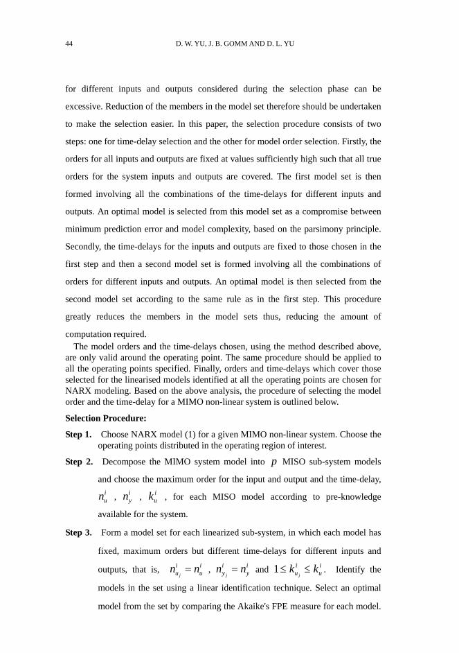
computation required. The model orders and the time-delays chosen, using the method described above,

are only valid around the operating point. The same procedure should be applied to all the operating points specified. Finally, orders and time-delays which cover those selected for the linearised models identified at all the operating points are chosen for NARX modeling. Based on the above analysis, the procedure of selecting the model order and the time-delay for a MIMO non-linear system is outlined below.

Selection Procedure:

Step 1. Choose NARX model (1) for a given MIMO non-linear system. Choose the operating points distributed in the operating region of interest.

Step 2. Decompose the MIMO system model into MISO sub-system models

and choose the maximum order for the input and output and the time-delay,

, , , for each MISO model according to pre-knowledge

available for the system.

p

nui ny

i kui

Step 3. Form a model set for each linearized sub-system, in which each model has

fixed, maximum orders but different time-delays for different inputs and

outputs, that is, n nui

ui

j= , n ny

iyi

j= and 1≤ ≤k ku

iui

j. Identify the

models in the set using a linear identification technique. Select an optimal

model from the set by comparing the Akaike's FPE measure for each model.


This is the selection of the time-delay.

Step 4. Form a model set for each linearised sub-system in which each model has

the fixed time-delay selected in Step 3 but different orders for the input

and output, that is, 1≤ ≤n nui

ui

j , 1≤ ≤n ny

iyi

j and fixed k . Identify

the models in the set using a linear identification technique. Select an

optimal model from the set by comparing the Akaike's FPE measure for

each model. This is the selection of the system order.

ui

j

Step 5. Repeat Step 3 to Step 4 for all the operating points chosen. Compare the chosen linear model orders and the time-delays for all the operating points, l . The NARX model order and the time-delay should be chosen to include all identified terms in the selected linear ARX models over the operating region considered.

It should be noted that the linearization discussion in this method has not assumed any particular non-linear identification technique. Therefore, the method is also applicable to any approach used to approximate the NARX model, such as different types of neural network, a fuzzy model or polynomial expansion.

It is known that, in neural network modeling, a constant or nearly constant input can be represented by a bias input. On the other hand, if the partial differentiation of the non-linear function, f ( )• in equation (1), with respect to one of its variables is zero, then the function will not change along the direction of this variable. It follows that even if the model order and time-delay identified using this method are not the true ones of the non-linear system, because of missing terms caused by zero or nearly zero gradient over the operating region considered, the order and time-delay are still appropriate for neural modeling as the effect of the missing terms can be realized by the bias input of the neural network.

3. Model order and time-delay selection for a MIMO CSTR process

The model order and time-delay selection method described in Section 2 is applied to a non-linear, multivariable CSTR process to demonstrate the selection procedure and the effectiveness of the method. It is followed by the modeling of the process using one of the possible intelligent methods, neural networks, according to the order and the time-delay selected using the proposed method.

3.1 The CSTR process

The CSTR process investigated here is a typical chemical process employed as a test bed by many researchers. The process is shown in Figure 1 and is similar to that described by Foss and Johansen [8]. In Fig.1, (T), (A) and (C) denote transducers, actuators and control, respectively. The process consists of a simulated continuous stirred tank reactor in which a second order endothermic chemical reaction 2A→B takes place. The reactor level is maintained at a constant set point by a digital PI controller. The process was simulated using SIMULINK according to the following mass and energy balances,


(13) A dhdt

q hRi

v

= − ,

(14) Ahdcdt

c q c q Ahk c E RTAAi i A A A r= − − −0 0

22 exp( / ),

(15)

ρ ρr rr

r r i i r A A r h r r xc AhdTdt

c q T q T HAhk c E RT U T T U T T= − − − + − − −( ) exp( / ) ( ) ( )0 02

1 2∆ ,

(16) ρh h hh

h rV c dTdt

Q U T T= − −1( ) .

cA(T)

cAi(T)

Ti(T)

Th(T)Tr(T)

h(T)

h(C)

Q(A)

stir

Rv(A)

qi(A)

Fig.1 Simulated CSTR process

Descriptions of all quantities in equations (13)-(16) are given in the Appendix. The main process disturbances were simulated as zero-mean Gaussian distributed fluctuations on the inflow rate, inflow concentration and the inflow temperature. Measurement noise was simulated as zero-mean Gaussian white noise added to the reactor liquid level, concentration and temperature. Two inputs and two outputs are chosen for the process to be

⎥⎦

⎤⎢⎣

⎡=

Qq

u i , . ⎥⎦

⎤⎢⎣

⎡=

r

A

Tc

y

Since the liquid level, h, is not coupled with the concentration and temperature in equation (13) and it is maintained constant, the liquid level dynamics is simply a first order system, and therefore the modeling of the liquid level is not considered here. The process is decomposed into two MISO sub-systems of the concentration and the temperature, which can be represented in the following form

c f q Q T tA i r= 1( , , , ), T f q Q c tr i A= 2 ( , , , ).


From equations (14) and (15) it is known that non-linearity is involved in both the dynamics and steady states of the reactor concentration and temperature. In the following sub-section, the proposed method will be used to select the order and time-delay for NARX modeling of the CSTR process.

3.2 Order and time-delay selection

The order and time-delay selection method is applied to the CSTR process. The selection follows the procedure given in Section 2. Firstly, two operating points for each of the two inputs are chosen to be = 2.5, 3.5 l/s for the operating range (2, 4) l/s and ( = 400, 600 kW for the operating range (300, 700) kW. Consequently, four operating points are formed in the two dimensional input space from the combinations of the operating points for each input variable:

( )qi 0

)Q 0

⎥⎦

⎤⎢⎣

⎡=

6005.3

4005.3

6005.2

4005.2

0U .

At each operating point, input and output data were collected from the SIMULINK model of the CSTR process. In order to minimize the excitation of the process non-linearity, for linear identification, the excitation signal for each operating point is chosen to be a random binary sequence (RBS) with small amplitude in the range

u u u0 01 0 01 1 0 01( . ) ( . )− ≤ ≤ + ,

where is the element of U at an operating point. It was considered that an RBS with large amplitude would excite the non-linearity of the process, so that the identification of the linearised equation would not be precise. On the other hand, if the amplitude of the RBS excitation signal was chosen too small, the signal-to-noise ratio would be low due to the disturbances and noise subjected by the process, so that the identification of the linearised equation was also not precise. Considering the two aspects of inquiry, a compromise RBS amplitude was chosen as the above. The sampling interval was chosen as T

u0 0

= 200sec according to the dynamics of the process where a rule of approximately 1/10 of the rise time to a step input was applied. Two hundred samples of process input and output data were collected at each operating point and used in the identification of the linearised models.

The MIMO CSTR process was decomposed into two MISO sub-systems, formulating the following model equations,

(17) c t f c t c t n T t k T t k nA A A c r Tr r Tr c( ) ( ( ), , ( ), ( ), , ( ),A A

= − − − − − +11 1 1 11 1L L

),())1(,),(),1(,),( 1111111 tenktQktQnktqktq QQQqqiqi iii

++−−−+−−− LL

(18) T t f T t T t n c t k c t k nr r r T A c A c cr A A A( ) ( ( ), , ( ), ( ), , ( ),= − − − − − +2

2 2 2 21 1L L


).())1(,),(),1(,),( 2222222 tenktQktQnktqktq QQQqqiqi iii

++−−−+−−− LL

Secondly, following Step 2 of the selection procedure, the maximum values of ,

and were chosen to be

ny

nu k

(19) ( )maxny = 3, ( )maxnu = 3, kmax = 3.

Following Step 3, for the linearised form of the MISO sub-system model (17), a model set, Set 1, was formed by fixing the order of input and output to be the maximum values and the time-delay to be less than or equal to the maximum, namely,

(20) , nncA

1 3= Tr1 3= , nqi

1 3= , nQ1 3= , kTr

1 3≤ , kqi

1 3≤ , k . Q1 3≤

With this choice, the model set for each operating point then has 27 models. The batch least squares algorithm was used to estimate the parameters for each model in model Set 1, and the Akaike's FPE obtained for each model is displayed in Fig.2. The four curves in Fig.2 are for the four operating points. It can be seen in Fig.2 that for the four operating points, model numbers 1 to 12 give the lowest FPE values. Therefore, model number 1 was chosen which has the time-delay as below

(21) kTr1 1= , kqi

1 1= , kQ1 1= .

0 5 10 15 20 25 301.5

1.6

1.7

1.8

1.9

2

2.1x 10-9 time delay selection for reactor concentration

model number in the model set 1

Aka

ikes

FP

E

Fig.2 Akaike's FPE for reactor concentration models in Set 1 at four operating points A similar procedure was applied to the linearised form of the MISO sub-system

model (18). A model set, Set 2, was formed containing the same 27 models as used in model Set 1. The Akaike's FPE values for the different models in model Set 2 for the four operating points are displayed in Fig.3. It can be seen that model numbers 1 to 6 have the lowest FPE values and therefore, the time-delay in model number 1 was again chosen

(22) kcA

2 1= , kqi

2 1= , kQ2 1= .


The next step is to choose the model orders for the input and output. Following Step 4,

model Set 3 was formed for the reactor concentration by fixing kTr1 1= , ,

according to (21) and changing the order within n

kqi

1 1=

kQ1 1= cA

1 3≤ , nTr1 3≤ ,

, nnqi

1 3≤ Q1 3≤ . This model set has 81 models.

0 5 10 15 20 25 300.17

0.18

0.19

0.2

0.21

0.22time delay selection for reactor temperature


Aka

ikes

FP

E

Fig.3 Akaike's FPE for reactor temperature models in Set 2 at four operating points

0 10 20 30 40 50 60 70 80 901.45

1.5

1.55

1.6

1.65

1.7x 10-9 order selection for reactor concentration

Model number in the model set 3

Aka

ikes

FP

E

Fig.4 Akaike's FPE for reactor concentration models in Set 3 at four operating points

For each operating point the parameters of these models were estimated using the same sets of input-output data as for the time-delay selection. The Akaike's FPEs obtained are displayed in Fig.4.


0 5 10 15 201.48

1.5

1.52

1.54

1.56

1.58

1.6

1.62

1.64

1.66

1.68x 10-9 magnified view of Fig.4


Aka

ikes

FP

E

Fig.5 Magnified view of the FPEs for model set 3

For the four operating points, the FPEs obtained minimum values on model number 7. This can be seen more clearly in Fig.5 which is a magnified graph. Model number 7 has the order

(23) ncA

1 1= , nTr1 1= , nqi

1 3= , nQ1 1= .

Similarly, based on the linearised equation of the MISO sub-system model of reactor temperature (18), the orders of input and output were selected. Model set 4 was formed by fixing the time-delay

A , kqi

kc2 1= 2 1= , kQ

2 1= according to (22) and changing the input and the output orders within nTr

2 3≤ , , , n

ncA

2 3≤nqi Q

2 3≤ 2 3≤ . Therefore, model set 4 also has 81 models. Akaike's FPE for each estimated linear model in Set 4 are displayed in Fig.6 for the four operating points.

0 10 20 30 40 50 60 70 80 901.2

1.3

1.4

1.5

1.6

1.7

1.8

1.9Fig.7 Order selection for tank temperature

Model number in the model set 4

Aka

ikes

FP

E

Fig.6 Akaike's FPE for reactor temperature models in Set 4 at four operating points.

Fig.6 shows that model number 40 obtains the minimum FPE value for the four operating points, which has input and output orders

(24) nTr2 2= , n , n , ncA

2 2= qi

2 2= Q2 1= .


This can be seen more clearly in Fig.7. Combining all the terms in the linearised sub-system models selected at each operating point gives the time-delays (21), (22) and the orders (23), (24) for NARX modeling of the reactor concentration and temperature respectively using the proposed method. The time-delays selected match the time-delays in the original simulated model. The orders chosen are also reasonably consistent with the dynamics of the simulated model. In the following section, neural networks are employed to model the MIMO non-linear CSTR process based on the orders and time-delays chosen in this section.

25 30 35 40 451.2

1.3

1.4

1.5

1.6

1.7

1.8

1.9magnified view of Fig.6


Aka

ikes

FP

E

Fig.7 Magnified view of FPEs in model set 4

4. Neural nodeling of the CSTR process

In this section, neural modelling of the CSTR process in two different ways is described based on the orders and time-delays previously chosen. One way is to use two networks to model the two MISO sub-systems respectively (Section 4.1 and 4.2). The second way is to use one network to model the entire MIMO system (Section 4.4 ).

The network used was a radial basis function (RBF) network which performs a

non-linear mapping x yN p∈ℜ → ∈ℜ$ via the transformation,

(25) $y WT T= φ ,

(26) φ φ= = ∗ ∗( ) log( )d d d d ,

(27) d x ci i= −2 i nh= 1, ,L .

where and x are the network output and input vectors respectively; W

is the weighting matrix with element denoting the weight connecting the i

hidden node output to the network output;

$y n ph∈ℜ ×

wijth

j th φ ∈ℜnh is the output vector of the


non-linear function in the hidden layer, ∗ denotes the element array multiplying

operation; cinh∈ℜ is the i centre vector; n is the number of nodes in the

hidden layer; d is the i element of vector d. The weighting matrix, W, is

computed using a recursive least-squares algorithm (RLS) (Ljung and Soderstrom

[13]) such that the model prediction error is minimized. In order to improve the

accuracy of the neural model, normalization is made to the training data as well as

the test data in the following way,

thh

ith

x x xnor x traitrai= −( ) / ( )σ ,

where xtrai and σ x trai( ) are the mean value and the standard deviation of the

training data input, respectively. When the network is used after training, xtrai and

σ x trai( ) are used to restore the neural model output using a reverse formula

$ $ ( )y y xnor x trai trai= ∗ +σ .

The excitation signal used to generate the process input-output data for non-linear modeling was designed to cover the whole operating space. Here, a random step input series with the amplitude uniformly distributed in the region of

⎥⎦

⎤⎢⎣

⎡≤≤≤≤

=)(700300

)/(42kWQslq

u i

and with the hold on time uniformly distributed in the range of [1,7] was used. This excitation signal was used instead of the more common random amplitude series (RAS) with a fixed hold on time because a varying hold on time will excite more information of the process dynamics. The process disturbances and measurement noise are simulated by the same white noise as described in Section 3.1. The excitation signals and outputs of the process were collected for 900 samples with the sampling interval 200 sec, which is the same as that used for the order and time-delay selection. The first 800 data samples were used to train the RBF networks while the last 100 samples of data were used for cross validation of the neural models. All networks had 40 centers which were chosen using the k-means clustering method.

4. 1 Modeling reactor concentration

According to the order and time-delay chosen for the reactor concentration in

Section 3, kTr1 1= , kqi

1 1= , k in equation (21) and nQ1 1= cA

1 1= , nTr1 1= ,

, nnqi

1 3= Q1 1= , (1 1 3 1 ) in equation (23), the input vector to the network is


correspondingly formed as below with reference to equation (17),

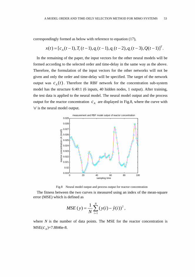
x t c t T t q t q t q t Q tA r i i iT( ) [ ( ), ( ), ( ), ( ), ( ), ( )]= − − − − − −1 1 1 2 3 1 .

In the remaining of the paper, the input vectors for the other neural models will be formed according to the selected order and time-delay in the same way as the above. Therefore, the formulation of the input vectors for the other networks will not be given and only the order and time-delay will be specified. The target of the network output was c . Therefore the RBF network for the concentration sub-system model has the structure 6:40:1 (6 inputs, 40 hidden nodes, 1 output). After training, the test data is applied to the neural model. The neural model output and the process output for the reactor concentration are displayed in Fig.8, where the curve with 'o' is the neural model output.

tA ( )

cA

0 20 40 60 80 1000.019

0.02

0.021

0.022

0.023

0.024

0.025

0.026

0.027

0.028

0.029measurement and RBF model output of reactor concentration

sampling time

reac

tor c

once

ntra

tion

cA (m

ol/l)

Fig.8 Neural model output and process output for reactor concentration

The fitness between the two curves is measured using an index of the mean-square error (MSE) which is defined as

MSE yN

y i y ii

N

( ) ( ( ) $( ))= −=∑1 2

1

,

where N is the number of data points. The MSE for the reactor concentration is MSE(c )=7.8846e-8. A


0 20 40 60 80 100320

330

340

350

360

370

380measurement and RBF model output of reactor temperature

sampling time

reac

tor t

empe

ratu

re T

r (K

)

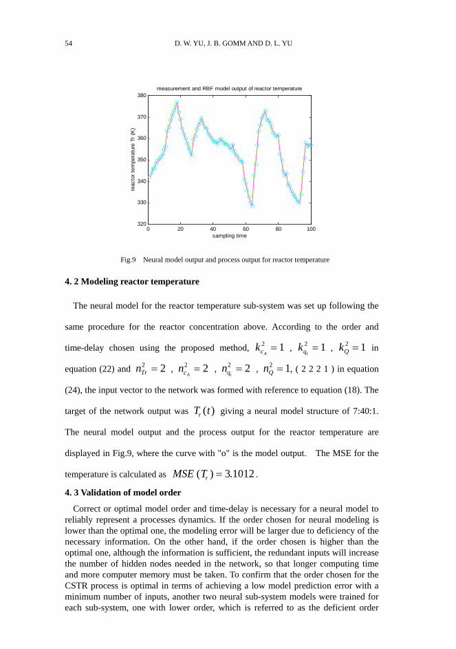
Fig.9 Neural model output and process output for reactor temperature

4. 2 Modeling reactor temperature

The neural model for the reactor temperature sub-system was set up following the

same procedure for the reactor concentration above. According to the order and

time-delay chosen using the proposed method, kcA

2 1= , kqi

2 1= , in

equation (22) and

kQ2 1=

nTr2 2= , ncA

2 2= , nqi

2 2= , nQ2 1= , ( 2 2 2 1 ) in equation

(24), the input vector to the network was formed with reference to equation (18). The

target of the network output was T tr ( ) giving a neural model structure of 7:40:1.

The neural model output and the process output for the reactor temperature are

displayed in Fig.9, where the curve with "o" is the model output. The MSE for the

temperature is calculated as MSE Tr( ) .= 3 1012 .

4. 3 Validation of model order

Correct or optimal model order and time-delay is necessary for a neural model to reliably represent a processes dynamics. If the order chosen for neural modeling is lower than the optimal one, the modeling error will be larger due to deficiency of the necessary information. On the other hand, if the order chosen is higher than the optimal one, although the information is sufficient, the redundant inputs will increase the number of hidden nodes needed in the network, so that longer computing time and more computer memory must be taken. To confirm that the order chosen for the CSTR process is optimal in terms of achieving a low model prediction error with a minimum number of inputs, another two neural sub-system models were trained for each sub-system, one with lower order, which is referred to as the deficient order


model, and the other with higher order, which is referred to as the redundant order model. The time-delays for these models remained the same as in the optimal order models (equations (21) and (22)).

For the reactor concentrationcA , the optimal order chosen for cA , Tr , q , Q was

( 1 1 3 1 ). The deficient order model used an order of ( 1 1 2 1 ) and the redundant

order model used an order of ( 2 2 3 1 ). For the reactor temperature, the optimal

order was chosen as ( 2 2 2 1 ) for

i

Tr , cA , , Q. The deficient order model used an

order of ( 2 2 1 1 ) and the redundant order model used an order of ( 3 2 2 2 ). The

same sets of training and test data and the same number of centers were used for the

two additional models of each variable. The MSEs of the sub-system model outputs

for the two variables are displayed in Table 1.

qi

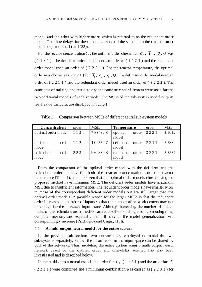
Table 1 Comparison between MSEs of different neural sub-system models

Concentration order MSE Temperature order MSE optimal order model 1 1 3 1 7.8846e-8 optimal order

model 2 2 2 1 3.1012

deficient order model

1 1 2 1 1.0055e-7 deficient order model

2 2 1 1 5.5382

redundant order model

2 2 3 1 9.6083e-8 redundant order model

3 2 2 1 3.5537

From the comparison of the optimal order model with the deficient and the

redundant order models for both the reactor concentration and the reactor temperature (Table 1), it can be seen that the optimal order models chosen using the proposed method have minimum MSE. The deficient order models have maximum MSE due to insufficient information. The redundant order models have smaller MSE to those of the corresponding deficient order models but are still larger than the optimal order models. A possible reason for the larger MSEs is that the redundant order increases the number of inputs so that the number of network centers may not be enough for the increased input space. Although increasing the number of hidden nodes of the redundant order models can reduce the modeling error; computing time, computer memory and especially the difficulty of the model generalization will correspondingly increase (Psichogios and Ungar, [15]).

4.4 A multi-output neural model for the entire system

In the previous sub-sections, two networks are employed to model the two sub-systems separately. Part of the information in the input space can be shared by both of the networks. Thus, modeling the entire system using a multi-output neural network based on the optimal order and time-delay selected has also been investigated and is described below.

In the multi-output neural model, the order for ( 1 1 3 1 ) and the order for cA Tr

( 2 2 2 1 ) were combined and a minimum combination was chosen as ( 2 2 3 1 ) for


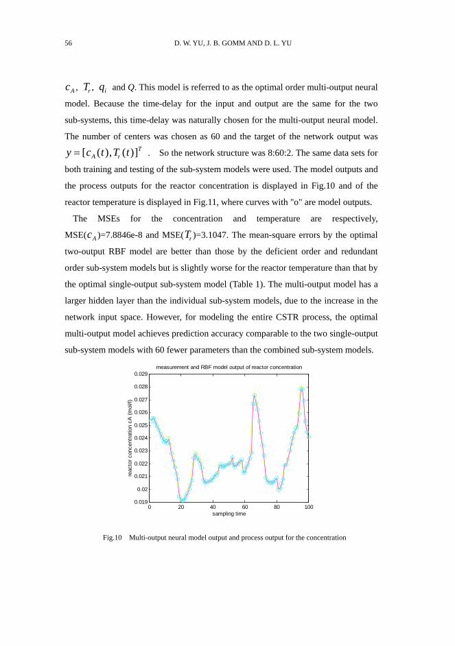
cA , Tr , and Q. This model is referred to as the optimal order multi-output neural

model. Because the time-delay for the input and output are the same for the two

sub-systems, this time-delay was naturally chosen for the multi-output neural model.

The number of centers was chosen as 60 and the target of the network output was

qi

y c t T tA rT= [ ( ), ( )] . So the network structure was 8:60:2. The same data sets for

both training and testing of the sub-system models were used. The model outputs and

the process outputs for the reactor concentration is displayed in Fig.10 and of the

reactor temperature is displayed in Fig.11, where curves with "o" are model outputs.

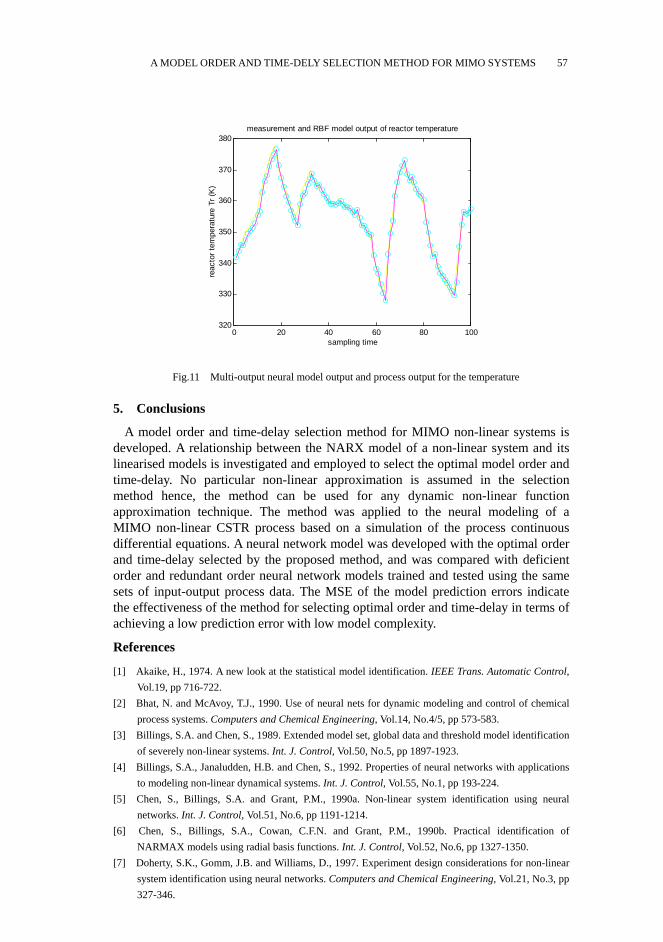
The MSEs for the concentration and temperature are respectively,

MSE(cA )=7.8846e-8 and MSE(Tr )=3.1047. The mean-square errors by the optimal

two-output RBF model are better than those by the deficient order and redundant

order sub-system models but is slightly worse for the reactor temperature than that by

the optimal single-output sub-system model (Table 1). The multi-output model has a

larger hidden layer than the individual sub-system models, due to the increase in the

network input space. However, for modeling the entire CSTR process, the optimal

multi-output model achieves prediction accuracy comparable to the two single-output

sub-system models with 60 fewer parameters than the combined sub-system models.

0 20 40 60 80 1000.019

0.02

0.021

0.022

0.023

0.024

0.025

0.026

0.027

0.028

0.029measurement and RBF model output of reactor concentration

sampling time

reac

tor c

once

ntra

tion

cA (m

ol/l)

Fig.10 Multi-output neural model output and process output for the concentration


0 20 40 60 80 100320

330

340

350

360

370

380measurement and RBF model output of reactor temperature

sampling time

reac

tor t

empe

ratu

re T

r (K

)

Fig.11 Multi-output neural model output and process output for the temperature

5. Conclusions

A model order and time-delay selection method for MIMO non-linear systems is developed. A relationship between the NARX model of a non-linear system and its linearised models is investigated and employed to select the optimal model order and time-delay. No particular non-linear approximation is assumed in the selection method hence, the method can be used for any dynamic non-linear function approximation technique. The method was applied to the neural modeling of a MIMO non-linear CSTR process based on a simulation of the process continuous differential equations. A neural network model was developed with the optimal order and time-delay selected by the proposed method, and was compared with deficient order and redundant order neural network models trained and tested using the same sets of input-output process data. The MSE of the model prediction errors indicate the effectiveness of the method for selecting optimal order and time-delay in terms of achieving a low prediction error with low model complexity.

References

[1] Akaike, H., 1974. A new look at the statistical model identification. IEEE Trans. Automatic Control, Vol.19, pp 716-722.

[2] Bhat, N. and McAvoy, T.J., 1990. Use of neural nets for dynamic modeling and control of chemical process systems. Computers and Chemical Engineering, Vol.14, No.4/5, pp 573-583.

[3] Billings, S.A. and Chen, S., 1989. Extended model set, global data and threshold model identification of severely non-linear systems. Int. J. Control, Vol.50, No.5, pp 1897-1923.

[4] Billings, S.A., Janaludden, H.B. and Chen, S., 1992. Properties of neural networks with applications to modeling non-linear dynamical systems. Int. J. Control, Vol.55, No.1, pp 193-224.

[5] Chen, S., Billings, S.A. and Grant, P.M., 1990a. Non-linear system identification using neural networks. Int. J. Control, Vol.51, No.6, pp 1191-1214.

[6] Chen, S., Billings, S.A., Cowan, C.F.N. and Grant, P.M., 1990b. Practical identification of NARMAX models using radial basis functions. Int. J. Control, Vol.52, No.6, pp 1327-1350.

[7] Doherty, S.K., Gomm, J.B. and Williams, D., 1997. Experiment design considerations for non-linear system identification using neural networks. Computers and Chemical Engineering, Vol.21, No.3, pp 327-346.


[8] Foss, B.A. and Johansen, T.A., 1992, An integrated approach to on-line fault detection and diagnosis -- including artificial neural networks with local basis functions. Proc. IFAC Symposium on On-line Fault Detection and Supervision in the Chemical Process Industries, Newark, USA, April 22-24, pp 207-212.

[9] Gomm, J.B., Williams, D., Evans, J.T., Doherty, S.K. and Lisboa, P.J.G. 1996a. Enhancing the non-linear modeling capabilities of MLP neural networks using spread encoding. Fuzzy Sets and Systems, Vol.79, No.1, pp 113-126.

[10] Gomm, J.B., Yu, D.L. and Williams, D., 1996b. A new model structure selection method for non-linear systems in neural modeling. Proc. UKACC Int. Conf. Control'96, 2-5 Sept., Exeter, UK, pp 752-757.

[11] Hunt, K.J., Sbarbaro, D., Zbikowski, R. and Gawthrop, P.J., 1992. Neural networks for control systems -- a survey. Automatica, Vol.28, No.6, pp 1083-1112.

[12] Leontaritis, I.J. and Billings, S.A., 1987. Model selection and validation methods for non-linear systems. Int. J. Control, Vol.45, No.1, pp 311-341.

[13] Ljung, L. and Soderstrom, T., 1983. Theory and practice of recursive identification. MIT Press, Cambridge MA.

[14] Narendra, K.S. and Parthasarathy, K., 1990. Identification and Control of dynamic systems using neural networks. IEEE Trans. Neural Networks, Vol.1, pp 4-27.

[15] Psichogios, D.C. and Ungar, L.H., 1994. SVD-NET: an algorithm that automatically selects network structure. IEEE Trans. Neural Networks, Vol.5, No.3, pp 513-515.

[16] Yu, D.L., Shields, D.N. and Daley, S., 1996. A hybrid fault diagnosis approach using neural networks. Neural Computing & Applications, Vol.4, No.1, pp 21-26.

Appendix 1

The meaning of the quantities in the CSTR model of equations (13) -- (16) are defined as follows.

qi reactor inflow h liquid level q0 reactor outflow Vh effective volume of

heat exchanger Rv outflow pipe resistance due to

control valve

A reactor cross-sectional

area cA concentration of component A in

reactor cAi

concentration of

component A in inflow k0 frequency factor E A activation energy

R universal gas constant Tr reactor temperature ρr mass density in reactor cr specific heat capacity in

reactor ρh mass density in heat exchanger ch specific heat capacity in

heat exchanger Ti inflow temperature ∆H reaction energy


U1 heat transmission coefficient

between heat

Th temperature of heat

exchanger medium

exchanger and reactor Tx environment

temperature U2 heat transmission coefficient

between reactor and environment

Q heating power

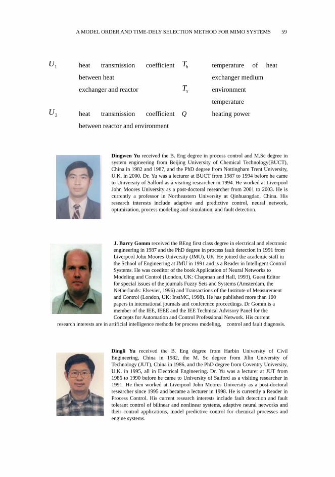
Dingwen Yu received the B. Eng degree in process control and M.Sc degree in system engineering from Beijing University of Chemical Technology(BUCT), China in 1982 and 1987, and the PhD degree from Nottingham Trent University, U.K. in 2000. Dr. Yu was a lecturer at BUCT from 1987 to 1994 before he came to University of Salford as a visiting researcher in 1994. He worked at Liverpool John Moores University as a post-doctoral researcher from 2001 to 2003. He is currently a professor in Northeastern University at Qinhuangdao, China. His research interests include adaptive and predictive control, neural network, optimization, process modeling and simulation, and fault detection.

J. Barry Gomm received the BEng first class degree in electrical and electronic engineering in 1987 and the PhD degree in process fault detection in 1991 from Liverpool John Moores University (JMU), UK. He joined the academic staff in the School of Engineering at JMU in 1991 and is a Reader in Intelligent Control Systems. He was coeditor of the book Application of Neural Networks to Modeling and Control (London, UK: Chapman and Hall, 1993), Guest Editor for special issues of the journals Fuzzy Sets and Systems (Amsterdam, the Netherlands: Elsevier, 1996) and Transactions of the Institute of Measurement and Control (London, UK: InstMC, 1998). He has published more than 100 papers in international journals and conference proceedings. Dr Gomm is a member of the IEE, IEEE and the IEE Technical Advisory Panel for the Concepts for Automation and Control Professional Network. His current

research interests are in artificial intelligence methods for process modeling, control and fault diagnosis.
Dingli Yu received the B. Eng degree from Harbin University of Civil Engineering, China in 1982, the M. Sc degree from Jilin University of Technology (JUT), China in 1986, and the PhD degree from Coventry University, U.K. in 1995, all in Electrical Engineering. Dr. Yu was a lecturer at JUT from 1986 to 1990 before he came to University of Salford as a visiting researcher in 1991. He then worked at Liverpool John Moores University as a post-doctoral researcher since 1995 and became a lecturer in 1998. He is currently a Reader in Process Control. His current research interests include fault detection and fault tolerant control of bilinear and nonlinear systems, adaptive neural networks and their control applications, model predictive control for chemical processes and engine systems.


Department of Automation, Northeastern University at Qinhuangdao, Qinhuangdao, Hebei Province, P.R. China, 066004

email: [email protected] Department of Engineering, Liverpool John Moores University, Byrom street, Liverpool, L3 3AF, UK email: [email protected]

mailto:[email protected]

mailto:[email protected]

a model order and time-delay selection … stirred tank reactor (cstr) ... neural network modelling,...

Documents