1

Time Course Experiments

Biostatistics 140.688Rafael A. Irizarry

Today materialcourtesy of Terry Speed

2

Outline

Types and featuresDesign, including replication

(with examples)Identifying the genes of interest

(with examples)

Types and features of microarraytime course experiments

2

4

Types/features

• Typically short series: k = 4-10 time points forshorter,and 11-20 time points for longer series; oftenirregularly spaced; with no or few (< 5) replications.

• Can be periodic, as in the cell cycle: Cho et al.(1998), Spellman et al.,(1998), or circadian rhythms,Storch et al. (2002),

OR• May have no particular pattern, as in developmental

time courses: Chu et al. (1998), Wen et al. (1998),Tamayo et al. (1999).

5

Types/features, cont.

• May be longitudinal, where mRNA samples atdifferent times are extracted from the same unit (cellline, tissue or individual), but more commonly cross-sectional, where mRNA samples are from differentunits.

• Gene expression values at different time points maybe correlated, especially in a longitudinal study, orwhen a common reference design is used for a cross-sectional study. At other times, the experimentaldesign induces correlations in cross-sectional studies.

6

Types/features, completed.

• Two general types of hypotheses of interest: the one-sample (or one-class) problem: which genes

are changing in time? and the 2 or >2 sample (orclass) problem: which genes are changing differentlyin time across the samples (or classes)?

• Two broad types of mRNA samples: from cells or celllines which give reasonably repeatable responseswithin classes, and whole organism (mice, humans),where there is a lot of response variability withinclasses.

3

Design of microarray timecourse experiments

8

Most important issues

The first issue is: longitudinal or cross-sectional? The questionrevolves on whether it is important to measure change withinunits.

For two-channel (cDNA or long oligo) arrays, a major question iswhether or not to use a reference design. Most frequently, theanswer is yes.

For very short two-channel time courses, the possibility arises ofoptimizing the design for contrasts of interest.

Important design issues include not just assignment of mRNA toarrays, but also the actual conduct of the experiment, includingpreparation of the sample mRNA, the times of hybridizations,and the equipment, reagents and personnel used.

9

First illustrative example:A plant’s response to a pathogen.

.

Healthy Arabidopsis thaliana (mustard weed) plant

4

10

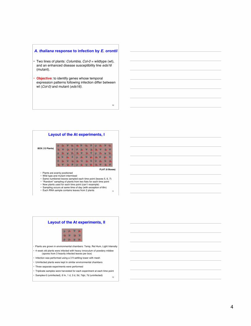
A. thaliana response to infection by E. orontii

• Two lines of plants: Columbia, Col-0 = wildtype (wt),and an enhanced disease susceptibility line eds16(mutant).

• Objective: to identify genes whose temporalexpression patterns following infection differ betweenwt (Col-0) and mutant (eds16).

11

1616

1616

1616 16

1616

1616

1616

1616

1616

1616

16

1616

1616

161616

1616

1616

1616

1616

1616

1616

BOX (12 Plants)

FLAT (6 Boxes)• Plants are evenly positioned• Wild type and mutant intermixed• Same numbered leaves sampled each time point (leaves 5, 6, 7) • “Random” sampling of plants from two flats for each time point• New plants used for each time point (can’t resample)• Sampling occurs at same time of day (with exception of 6hr)• Each RNA sample contains leaves from 2 plants

Layout of the At experiments, I

12

1616

1616

1616

Layout of the At experiments, II

• Plants are grown in environmental chambers: Temp, Rel Hum, Light Intensity

• 4 week old plants were infected with heavy innoculum of powdery mildew(spores from 3 heavily infected leaves per box)

• Infection was performed using a 3 ft settling tower with mesh

• Uninfected plants were kept in similar environmental chambers

• Three separate experiments were performed

• Triplicate samples were harvested for each experiment at each time point

• Samples-0 (uninfected), 6 hr, 1 d, 3 d, 5d, 7dpi, 7d (uninfected)

5

13

Kandel, Schwarz, and Jessel; 1991

Second illustrative exampleOligodendrocytes (OL) myelinate Central Nervous Systemaxons……and develop from migrating oligodendrocyteprecursor cells (OPC)

14

The development from OPC to OL in vitro

We study this phase

15

Purpose of OPC/OL experiment

• Broad purpose: to examine gene regulation in culturedoligodendrocyte precursor cells (OPC) as they develop intooligodendrocytes (OL).

• Narrower purpose: to identify a subset of genes withup-regulated timecourses. Candidate genes predictedto be secreted will be assayed for their ability to clustersodium channels along cultured retinal ganglion axons.

6

16

Day 0 Proliferation media

PurifiedOPCprepfrom P7rat pups

Day 1*Differentiationmedia

mRNA collected

Day 2*

mRNA collectedDay 3*

mRNA collected

Day 4*

mRNA collected

Differentiationmedia Day 6*

mRN collected

Day 8*

mRNA collected

Day 10*

mRNA collected

Day 13*

mRNA collected

Day7

Differentiationmedia

Differentiationmedia

OPC/OL experiment: RNA sample preparation

17

Back to generalities: ReplicationWe can have biological, technical and probe set (spot) replicatesReplication is a good thing. With it we get estimates of variability

relative to which temporal changes and/or conditiondifferences can be assessed.

Biological replicates are best, as they permit conclusions to beextrapolated, something not possible with tech. reps.

With unreplicated experiments, inference to a wider populationis not possible, and analysis is less straightforward, beingdependent on unverifiable assumptions, as no estimate ofpure error is available.

When we do have replicates, it is better to use the variationbetween them in the analysis, and not simple average them.

Today I will discuss only replicated time course experiments.

18

Replication in the At experiments

• Three experiments - effectively biological replicates - wereconducted using the wt and mutant lines, and within each, 3technical replicate series. Not all have been hybridized tochips. Later we use one series from experiments I and III, andtwo from experiment II.

• These experiments are longitudinal at the level of experiment,but cross-sectional at the level of mRNA sample (fromseparate leaves). The blurring of these distinctions is notunusual.

7

19

d0 d1* d2* d3* d4* d5 d6* d7 d8* d9 d10* d11 d12 d13*

mRNA samples at the 8 *-d time points were collected

4 independent preparations were performed, each of whichgenerated mRNA for every time point. We view this as 4biological replicates of a longitudinal study. Again it is notclearcut. For each biological replicate, a dye-swap pair oftechnical replicates was done.

Proliferation mediadifferentiation media

differentiation media

differentiation media

differentiation media

Replication in the OPC/OL experiment

20

Hybridizations for the At experiments

• Initially we hybridized mRNA from just one of the technicalreplicate series from experiments I and III, and two fromexperiment II.

• The Affymetrix Arabidopsis 24K GeneChip® was used. In all2(genotypes)x6(times)x4(experiments) = 48 chips werehybed.

In addition, data from 2(genotypes)x4(experiments) = 8 chipsfor day 7 uninfected samples are plotted.

• Low level analysis (background, normalization, probe setsummarization) done by RMA.

21

Pooling in the OPC/OL experiment

d1 d2 d3 d4 d6 d8 d10 d13

Reference poolsamples for this prep

Individualtime pointsamples

pooling

Each prep has its own reference pool, which is the pool ofall the individual time point mRNA samples of that prep.

8

22

Statistical question for At experiments:

Find genes whose expression profiles differ between genotypes?

Profiles differlog2intensity

days

wt

mutant

Extra dots at day 7 from uninfected samples.

23Change over time No change over time

Statistical question for the OPC/OL experiment

Find genes whose expression levels change over time?

M M

day day

Identifying the genes of interest

ClusteringPairwise comparisons

ANOVA with time as a factorEmpirical Bayes methods

9

25

Clustering with time-course data:brief literature review

Clustering methods have been widely used in this context to findgroups of genes with interesting and similar patterns.

Hierarchical clustering: Eisen et al (1998)

Self-organizing maps: Tamayo et al (1999), Saban et al (2001),Burton et al (2002).

k-means clustering: Tavazoie et al (1999)

Bayesian model-based clustering: Bar-Joseph et al (2002, 2003),Ramoni et al (2002)

HMM clustering: Schliep et al (2003).

26

Some drawbacks of clustering methods

They make no explicit use of the replicate information. Theyeither use all the slides or means of the replicates.

Clustering does not provide a ranking for the individual genesbased on the magnitude of change in expression levels overtime.

When the number of genes becomes large, clusteringmethods may not provide clear group patterns.

Cluster analysis may fail to detect changing genes thatbelong to clusters for which most genes do not change(Bar-Joseph et al. 2003).

There is the perennial question: How many clusters?

27

Hierarchical clustering of the top 500 genesOPC/OL expt, filtered by their variance

10

28

Cluster 6 One gene from the cluster

dayday

M M

29

Cluster 7 One gene from the cluster

30

Pairwise comparisons

One strategy is to make many or all univariate pairwisecomparisons, e.g. of consecutive times: days

1 vs 2, 2 vs 3, 3 vs 4, 4 vs 6, 6 vs 8, 8 vs 10, 10 vs 13

Illustration on the OPC/OL data: t-tests, univariateposterior odds : e.g. the LOD statistic, Lönnstedt andS (2002), Smyth (2004), the moderated t statistic,Smyth (2004),

11

31

Use of moderated t and posterior odds (LOD)

!

t*

2

=M

2

s*

2

/n

!

LOD = c +n + "

2

#

$ %

&

' ( log10

t*2

+ n )1+ "

t*2 1/n

1/n +1/*+ n )1+ "

+

,

- -

.

- -

/

0

- -

1

- -

!

s*

2

=(n "1)s

2

+ #$2

n "1+ #

Moderated s2 of M values Moderated t

Log10 of posterior odds against differential expression

32

| M |>1

|t|>3

LOD>-2

| M|>1 & |t|>3 & LOD>-2

OPC/OL experiment: day 6 vs. day 4

LOD

M

33

The 14 highlighted genes

12

34

Pairwise comparisons: some drawbacks

As the previous slide shows, the strategy works, but….

• It involves a large number of tests for each gene, and there areover 10,000 genes in a typical microarray experiment: a two-way multiple testing problem.

• Merging all the lists of genes can be a tricky problem.

• We still cannot rank the genes according to the overall amountof change, which is often felt to be desirable.

35

ANOVA with time as a factor

At experiment: treat time and genotypes as factors with 6and 2 levels, resp., and form the ratio of the times xgenotypes MS to residual MS, giving an F5,d under the null,where d = 2×6×(4-1) = 36 are the residual d.f. Since there ispairing of wt and mutant, we should include that too, givinga kind of split-plot anova with 3 d.f. for reps, and 33 residuald.f., with times, genotypes and times x genotypes as before.

OPC/OL experiment: here we simply regard the 8 times asdefining 8 “groups”, and use anova to test the hypothesis ofall times means being equal, 4 replicate measurements foreach time (“group”).

36

Drawbacks with ANOVA

First, this approach does not deal adequately withcorrelations across time, if the experiment have alongitudinal component.

Second, just as with the t-statistic we illustrated in thepariwise comparisons, an element of moderation isdesirable.

Despite these reservations, anova can and does providean adequate analysis, although we feel it can beimproved by attempting to deal with the above twoissues.

One further point is this: with cross-sectional data, we caninclude regression modelling under the heading ofanova, see later.

13

37

In general, what do we want?

We prefer a formula to rank genes, in order to

• find those changing or not similarly expressed• provide a cut off for clustering

We feel that this formula should be

• t-like or F-like,i.e. involve standardized measures of effects,• multivariate, where appropriate, and• moderated.

38

Why moderation?

• We seek genes with large absolute or relativeamounts of change over time, in relation to theirreplicate variances, and covariances whererelevant.

• Variances and covariances are poorly estimatedin this context.

• Some sort of smoothing, borrowing strength, orempirical Bayes approach is called for.Simulations show that this helps, i.e. doing soimproves the identification of genes of interest.

• We use multivariate normals with conjugatepriors, as we want usable formulae, and not tohave to use MCMC.

Multivariate approaches forlongitudinal time course experiments

Here we treat one entire seriesas a random k-vector

14

40

Notation and models

We denote by Xg,1,…, Xg,n the replicate random k-vectorsrepresenting the observed time series for a single gene.

For the At data, n = 4 and k = 6, and the Xg,i,t are differencesof log intensities, i.e. log ratios of mutant to wt.

For the OPC/OL data, n = 4 and k = 8, and the Xg,i,t arelog ratios of experimental to reference pool intensities.

Our underlying model is that these Xg,i are i.i.d. N(µg,Σg),and we make different assumptions about µg and Σg.

41

Hypotheses

• With the At data, we are interested in testing the nullhypothesis Hg: µg = 0, Σg > 0, against the alternativeKg: µg ≠ 0, Σg > 0.

• With the OPC/OL data, we are interested in testing thenull hypothesis Hg: µg = constant, Σg > 0, against thealternative Kg: µg not constant, Σg > 0.

42

Notation and models, cont.

For our empirical Bayes (EB) approach, we have priors forµg and Σg reflecting the indicator status I = Ig of the gene,where Ig = 1 if Hg is true, and Ig = 0 otherwise, i.e. if Kg istrue.

We suppose that Pr(Ig =1) = p, independently for everygene, for a hyperparameter p, 0 <p <1.

From now on, we drop the subscripts g wherever possible.

15

43

Notation and models, completed With this background, our prior for Σ is inverse Wishart with

degrees of freedom ν and matrix parameter (νΛ)-1, where Λ> 0 is positive definite. When we are dealing with a varianceσ2, we use an inverse Gamma prior with analogousparameters λ2 and ν.

Our priors for µ will be different depending on whether I=0 orI=1, but in all cases are multivariate normal, and will involveΛ (or λ2 ). We omit the details.

Finally, the data X1,…, Xn are supposed i.i.d. given I, Σ andµ, with Xi | I, Σ, µ ~ N(µ , Σ ).

The multivariate normality assumption is reasonable, but notprecise. However, we judge our results by their utility, not ongoodness-of-fit of the models.

44

Summary of results for the At experiment; formulaefor the OPC/OL experiment are similar.

Our moderated S is

our moderated t-statistic is

Finally,

!

˜ t = n1/ 2 ˜ S

"1/ 2X .

!

˜ S = [E(" #1| S)]

#1=

(n #1)S + $%

n #1+ $,

!

O =P(I =1 | data)

P(I = 0 | data)=

p

1" p

#

$ %

&

' (

P(˜ t | I =1)

P(˜ t | I = 0)

is an increasing function of

We write MB = log10O for our multivariate B-statistic.

!

˜ T 2

= ˜ t ' ˜ t .

45

!

LR = 2(lK

max" l

H

max ) = n log(1+n

n "1X

TS"1

X )

= n log(1+ T2 /(n "1))

where S is assumed non " singular. Here T 2 is

Hotelling's statistic. In our case, n < k and S is

singular. If we plug in ˜ S , our moderated S, we get

the moderated Hotelling statistic, ˜ T 2, just seen.

Likelihood Ratio statistic

For the likelihood ratio (LR) test, we simply testthe null H against the alternative K in the usualway. We calculate:

16

46

Hyperparameter estimation

There are k(k+1)/2 + 3 parameters in the prior: Λ, p, ν, and η.

We simply choose p = 0.02, although clearly more could bedone here. Neither p nor η enter into .

Estimates of the hyperparameters ν and η are developedusing the univariate approach of Smyth (2004): η using thep/2 genes with the highest values, and ν using all thegenes. We omit the details.

Λ is estimated by the method of moments using the formula E(S) = (ν-k-1)-1νΛ.!

˜ T 2!

˜ T 2

Illustrative results for our At experiment

48

Estimate of Λ for the At experiment

100×SD: 14, 17, 15, 13, 16, 16.

Correlation matrix 1.00 .15 1.00 -.01 .15 1.00 .12 .07 .13 1.00 -.09 -.01 .02 -.02 1.00 .05 .06 .02 .15 -.16 1.00

17

Toprankedgenes

50

Illustrative results for our OPC/OL experiment

18

Evidence of autocorrelation

One gene’s sample covariance matrix:

2.67 2.40 2.36 1.31 1.63 0.04 -0.11 -0.69 2.40 2.17 2.14 1.20 1.48 0.05 -0.10 -0.61 2.36 2.14 2.18 1.25 1.57 0.07 -0.04 -0.53 1.31 1.20 1.25 0.74 0.93 0.06 0.00 -0.26 1.63 1.48 1.57 0.93 1.19 0.07 0.02 -0.31 0.04 0.05 0.07 0.06 0.07 0.01 0.02 0.02 -0.11 -0.10 -0.04 0.00 0.02 0.02 0.05 0.08 -0.69 -0.61 -0.53 -0.26 -0.31 0.02 0.08 0.25

If S=UDV’, D= diag(8.88, 0.37, 0.02, 0, 0, 0, 0, 0)

53

Another gene’s sample covariance matrix:

.83 .10 -.04 -.05 .19 .24 1.02 .69 .10 .03 .01 .03 .00 .01 .14 .04 -.04 .01 .05 .09 -.04 -.03 .00 -.07 -.05 .03 .09 .17 -.08 -.06 .04 -.11 .19 .00 -.04 -.08 .09 .09 .19 .21 .24 .01 -.03 -.06 .09 .11 .27 .26 1.02 .14 .00 .04 .19 .27 1.31 .80 .69 .04 -.07 -.11 .21 .26 .80 .66

If S=UDV’, D= diag(2.80,0.37,0.07,0, 0, 0, 0, 0)

Further evidence of autocorrelation

54

.10 .06 .05 .04 .03 .03 .03 .02 .06 .11 .06 .05 .04 .04 .04 .03 .05 .06 .11 .05 .04 .04 .04 .03 .04 .05 .05 .09 .04 .04 .04 .03 S = .03 .04 .04 .04 .09 .04 .04 .03 .03 .04 .04 .04 .04 .10 .05 .04 .03 .04 .04 .04 .04 .05 .09 .04 .02 .03 .03 .03 .03 .04 .04 .07

14.6 -4.6 -3.1 -1.5 -0.7 -0.3 -0.1 -0.3 -4.6 15.8 -3.3 -3.0 -1.4 -1.1 -1.3 -0.4 -3.1 -3.3 16.4 -3.1 -1.4 -1.5 -1.4 -1.7 -1.5 -3.0 -3.1 18.3 -3.0 -2.1 -2.1 -1.5S-1 = -0.7 -1.4 -1.4 -3.0 16.9 -2.5 -3.0 -1.0 -0.3 -1.1 -1.5 -2.11 -2.5 17.6 -4.8 -4.2 -0.1 -1.3 -1.4 -2.1 -3.0 -4.8 21.0 -5.9 -0.3 -0.4 -1.7 -1.5 -1.0 -4.3 -5.9 22.1

If S=UΛVT, Λ = diag(.38 .09 .06 .05 .05 .05 .04 .04), u1 = (.34 .41 .40 .37 .32 .37 .34 .27)T

Average single gene covariance matrix

19

Observations on autocorrelation

The correlation structure exhibited in the averagecovariance matrix resembles that of a slow movingaverage process, which is perhaps not surprisinggiven the way in which the samples of cells weretaken and the use of a common reference mRNAsource.

56

Toprankedgenes

Note that TC1 (red) does stand out

57

20

58

Conclusions

• Methods which rank genes (e.g. the MB statistic or themoderated Hotelling T2) perhaps provide easier access togenes whose absolute or relative expression varies overtime, than do multi-gene methods (e.g. cluster analysis).

• Among the single-gene methods, MB performs no worsethan other methods in both real data and simulated datacomparisons, and better than the F.

• The Hotelling T2 statistic is a viable alternative to MB,but we still need the moderated S.

• The MB statistic may be able to select interesting geneswhich are missed by other methods.

An important new paper

A Significance method for time CourseMicroarray Experiments Applied to TwoHuman Studies,JD Storey, JT Leek, W Xiao, JY Dai andRW Davis.

University of Washington BiostatisticsWorking Paper Series Paper 232, 2004.

60

Brief Summary, 1

Method developed for two human studies, both using the Affymetrixhuman U133A and 133B chips.

Endotoxin study, monitoring gene expression responses to bacterialendotoxin in blood leukocytes. Four subjects were administeredendotoxin, another four a placebo, and blood samples were taken at 2,4, 6, 9, and 24 hours after infusion.

Kidney aging study, to investigate changes in gene expression in thehuman kidney across different agess. Samples from normal kidneytissue removed at nephrectomy or renal transplant biopsy from 72patients with ages ranging from 27 to 92 years.

21

61

Brief Summary, 2

• The model used on each case has the following form forgene i on individual j at time t:

yij(t) = µi(t) + γij(t) + εij(t).

where the population average curve is µi(t) , individualsdeviate from the population average curve by γij(t), andmeasurement error and the remaining sources of variationare modelled by the εij(t). It is the γij(t) which distinguishesthis model from the ones we previously considered for modelorganisms with more repeatable expression profiles.

The observations are at times tij, and the µi(t) term ismodeled by cubic splines.

Software availability

Programs implementing our multivariate methodswill go into the open source R-based Bioconductor

package before the end of this summer.Available programs for some other approaches arelisted in the handout for this afternoon’s workshop.

63

Acknowledgements

Yu Chuan Tai, UC Berkeley

Mary Wildermuth, UC Berkeley

Jason Dugas, Stanford

Moriah Szpara, UC Berkeley & members of the Ngai lab

Gordon Smyth, WEHI

Monica Nicolau, Stanford University

22

64

Hybridizations for the OPC/OL experiments

The cDNA slides were made in the Ngai lab, UC Berkeley,using the RIKEN clone set, and the hybs done in ‘02/’03.

19,200 spots/slide, in 8x4 print-tip groups of size 25x24.Some genes were replicated: their M = log2R/G were averaged.Two dye-swap technical replicate slides run on mRNA from

each biological replicate: their M and -M were averaged.Time course (TC) 1 was done using slides from one batch,

while TC 2-4 used slides from another batch.The raw intensities were from an Axon scanner; the image

analysis was done by Spot using a morph background.Normalization was by print-tip lowess , followed by between

array MAD scale normalization for TC1, as there was a lotof variation across time in this replicate.

65

OPC/OL experiment: hybridization dates

2/8/03Cy5=time, Cy3=pool

2/6/03Cy5=pool, Cy3=time

TC4

2/10/03Cy5=pool, Cy3=time

12/10/02Cy5=time, Cy3=pool

TC3

1/14/03Cy5=time, Cy3=pool

12/3/02Cy5=pool, Cy3=time

TC2

4/11/02Cy5=time, Cy3=pool

4/4/02Cy5=pool, Cy3=time

TC1

Rep2Rep1

66

After NormalizationBefore Normalization

MA-plot for one hybridization in theOPC/OL experiment

vertical axis: M = log2R/G , horizontal axis: A = log2 √RG

23

67

QA/QC in the At experiments

In the At experiment, we checked the quality of allchips using fitPLM() in AffyExtensions. Wefound that 5 chips were of low quality, and thesewere repeated.

In addition the log2 intensities of replicate 1-3 wtday 3 sample were inconsistent with those fromthe other wt experiments for that day, despitehaving no obvious QC problems with the chips.These were “adjusted” using median polish onall the wt data.

68

QA/QC in the OPC/OL experiments

Here quality was a greater concern, no doubt as aresult of the wide spread of times over which thehybridizations were conducted. Also, the analysiswas done some time later, and there was nopossibility of repeating any of the hybridizations.

It turned out TC1 (data from a different chip batch)did stand out from the rest, but omitting thisreplicate was not an option, as there wereconcerns about aspects of the other hybridizationsas well: attenuated response range.

In the end, we relied on visual examination ofconsistency of responses, and qrt-pcr follow-up togive us confidence in our conclusions.