time …biomechanics.stanford.edu/paper/ijnme08a.pdf ·...

INTERNATIONAL JOURNAL FOR NUMERICAL METHODS IN ENGINEERINGInt. J. Numer. Meth. Engng 2008; 73:1413–1433Published online 9 July 2007 in Wiley InterScience (www.interscience.wiley.com). DOI: 10.1002/nme.2124

Time-dependent fibre reorientation of transversely isotropiccontinua—Finite element formulation and consistent linearization

G. Himpel1, A. Menzel2, E. Kuhl3 and P. Steinmann1,∗,†

1Chair of Applied Mechanics, Department of Mechanical and Process Engineering, University of Kaiserslautern,Kaiserslautern, Germany

2Institute of Mechanics and Control Engineering, Department of Mechanical Engineering, University of Siegen,Siegen, Germany

3Department of Mechanical Engineering, Stanford University, Palo Alto, CA, U.S.A.

SUMMARY

Transverse isotropy is realized by one characteristic direction—for instance, the fibre direction in fibre-reinforced materials. Commonly, the characteristic direction is assumed to be constant, but in somecases—for instance, in the constitutive description of biological tissues, liquid crystals, grain orientationswithin polycrystalline materials or piezoelectric materials, as well as in optimization processes—it provesreasonable to consider reorienting fibre directions. Various fields can be assumed to be the driving forcesfor the reorientation process, for instance, mechanical, electric or magnetic fields. In this work, we restrictourselves to reorientation processes in hyper-elastic materials driven by principal stretches.

The main contribution of this paper is the algorithmic implementation of the reorientation process intoa finite element framework. Therefore, an implicit exponential update of the characteristic direction isapplied by using the Rodriguez formula to express the exponential term. The non-linear equations onthe local and on the global level are solved by means of the Newton–Raphson scheme. Accordingly, thelocal update of the characteristic direction and the global update of the deformation field are consistentlylinearized, yielding the corresponding tangent moduli. Through implementation into a finite element codeand some representative numerical simulations, the fundamental characteristics of the model are illustrated.Copyright q 2007 John Wiley & Sons, Ltd.

Received 10 November 2006; Revised 21 May 2007; Accepted 21 May 2007

KEY WORDS: reorientation; transverse isotropy; fibre-reinforced materials

1. INTRODUCTION

Transverse isotropic materials, i.e. materials with one characteristic direction, can be found invarious fields of our daily life. In many cases the characteristic direction is fixed in the matrix

∗Correspondence to: P. Steinmann, Chair of Applied Mechanics, Department of Mechanical and Process Engineering,University of Kaiserslautern, D-67663 Kaiserslautern, Germany.

†E-mail: [email protected]

Copyright q 2007 John Wiley & Sons, Ltd.

1414 G. HIMPEL ET AL.

material, but in living materials, particularly, the characteristic direction changes due to changes intheir environments. These changes can be either smooth and continuous, for instance, in biologicalmaterials, or discontinuous, as in piezoelectric materials. One example for smoothly reorientingtransversely isotropic materials is biological soft tissue such as muscle tissue, cartilage tissueor our skin, where the characteristic directions, for instance, the muscle fibres or the collagenfibres, adapt their orientations to their mechanical loading environment. So far it is not clearlyinvestigated which are the driving forces for the reorientation process in biomaterials. Some authorsadvocate that principal stretches are the biological stimulus in soft tissues, see for instance, Driessenet al. [1–4], Kuhl et al. [5] and Menzel [6]. In Hariton et al. [7], stresses are chosen to drive thereorientation process. For a combined model of growth and reorientation, the reader is referred toImatani and Maugin [8] and Menzel [9]. Another example for reorienting transversely isotropicmaterials are liquid crystals, i.e. liquids with a crystalline structure. The physical condition ofthese materials is between the solid and the fluid phase. As is common in transversely isotropicmaterials, the characteristic direction of a liquid crystal is described by a position-dependentdirector. The most common application of liquid crystals is in liquid crystal displays, but theyare also a central component of biological systems, such as in myelin, DNS, protein and cellmembranes. Further, liquid crystals can be found in polymers, thermometers, pressure sensors, etc.For a broad outline of liquid crystals, the reader is referred to the book of Collings [10]. Drivingforces for the reorientation process in liquid crystalline materials, among others, are contact withother materials, electric or magnetic fields, see Ericksen [11].

To give another example on anisotropic reorienting materials, recall that piezoceramics can bepoled by displacements or electric fields, so that the polarization direction characterizes trans-versely isotropic material behaviour. Thereby, two fundamentally different piezoelectric effectscan be observed. The direct piezoelectric effect characterizes charging of the material caused byapplied stresses as, for instance, used in sensors. In actuators, the inverse piezoelectric effect isexploited, which means that an applied electric field induces mechanical strains. For a generalsurvey on piezoelectric materials, we refer to Kamlah [12] and Smith [13]. Due to mechanicalor electrical loading, switching of the polarization direction may be induced, where a differencebetween ferroelastic switching and ferroelectric switching is made. Ferroelastic switching refersto reorientation of domains under purely mechanical loading and ferroelectric switching refers toreorientation under electric loading, see, e.g. Schroder and Romanowski [14] and Arockiarajanet al. [15–17] and the references cited therein.

In general, reorientation phenomena can be observed in various polycrystalline materials, ofwhich metals are a classical example. Apart from texture evolution, for instance, related to theconstitutive behaviour within the individual grain, such grains might themselves reorient accordingto the overall loading conditions. In this regard, a thermodynamically consistent and stress-drivenframework has, among others, been proposed by Johansson et al. [18]. For a general survey, thereader is referred to the contributions in Kocks et al. [19].

Furthermore, simulations including reorienting characteristic directions can be used in the contextof optimization problems for composites, for instance, reinforced concrete in civil engineering orcarbon fibre-reinforced materials in motor sports, yachting, aircraft or wind engine construction,see for example, Pedersen [20]. For optimization problems, typically, principal stresses or strainsare assumed as driving forces.

It can be shown that for anisotropic elasticity the free energy reaches a critical state for commu-tating stresses and strains, see Vianello [21, 22] and Sgarra and Vianello [23]. Since the stressesand strains are coaxial if the characteristic direction is aligned with the principal stretch direction,

Copyright q 2007 John Wiley & Sons, Ltd. Int. J. Numer. Meth. Engng 2008; 73:1413–1433DOI: 10.1002/nme

FIBRE REORIENTATION OF TRANSVERSELY ISOTROPIC CONTINUA 1415

we postulate reorientation along the maximum principal strain direction. Furthermore, in this con-tribution, we restrict ourselves to hyper-elastic formats for the stress tensor. The major intentionof this paper is the derivation of a robust and efficient algorithmic formulation and its consistentlinearization within a finite element framework. In this context, we assume as an additional materialproperty a rotation of the characteristic direction, where in drilling rotations are excluded. Eventhough we will restrict ourselves to studying a specific constitutive model, the general algorithmicformulation can be applied to a wide range of applications. To be specific, the consistent lineariza-tion related to a reorienting fibre direction embedded into an iterative finite element context willbe useful for various types of adaptive materials as indicated above.

The paper is organized as follows: The constitutive framework for transversely isotropic materialsis summarized in Section 2. This includes the essential kinematic equations for finite deformationsas well as the constitutive description of transverse isotropy. In Section 3, essential equationsdescribing the reorientation process are derived. Firstly, the evolution in time of a line elementaccording to a rigid body motion is considered, later on to describe the evolution of the characteristicdirection driven by principal stretches. Section 4 contains the consistent linearization of the materialmodel, including an algorithmic update scheme for the characteristic direction as well as theincremental tangent modulus. In the last section, we discuss the material model by means ofnumerical examples. Firstly, the material behaviour is demonstrated by a simple tension test beforewe apply the theory to a homogeneous and an inhomogeneous boundary value problem. The papercloses with a short conclusion in Section 6.

2. CONSTITUTIVE FRAMEWORK

In this section, we summarize in brief the essential kinematics for the non-linear deforma-tion problem, as well as the constitutive equations for transversely isotropic hyper-elasticity.For a detailed overview on non-linear continuum mechanics, we refer to the monographs byChadwick [24] and Holzapfel [25].

2.1. Essential kinematics

Let X and x denote the placements of a particle in the material and the spatial configurations B0and Bt at times t0 and t , respectively, and u the appropriate non-linear deformation map

x=u(X, t) (1)

The corresponding deformation gradient

F=∇Xu(X, t) (2)

describes the tangent map from the material tangent space TXB0 to the spatial tangent space TXBtand J := detF>0 is the Jacobian. As a deformation measure, we introduce the right Cauchy–Greentensor in the material configuration

C=Ft · F=3∑

I=1�CI n

CI ⊗ nCI (3)



with nCI denoting the principal stretch direction associated with the principal stretch �CI , whereby,in this contribution we sort the principal stretches such that the index I increases with increasingprincipal stretch, namely

nCI · nCJ = �I J , �C1 ��C2 ��C3 (4)

To describe the evolution in time of the spatial line element with respect to the spatial line elementitself

dx= �x�x· dx=∇xv · dx (5)

the spatial velocity gradient can be introduced as

l=∇xv= F · F−1 (6)

with ˙{•}= �t {•}|X characterizing the material time derivative of a quantity {•} and v= x being thespatial velocity.

2.2. Transversely isotropic hyper-elasticity

For the representation of transverse isotropy, it is common practice to introduce the characteristicdirection nA in the material configuration or rather the sign-independent structural tensor A,whereby in this contribution the characteristic direction is assumed to be a non-constant, reorientingunit vector

A=nA⊗ nA with nA · nA= 1 and nA �= const (7)

The characteristic direction describes, for instance, the fibre direction in a fibre-reinforced materialor the collagen fibres in the arterial wall. Thus, the evolution of the characteristic direction mustbe orthogonal to the characteristic direction itself

d

dt(nA · nA)= 0 �⇒ nA · nA= 0 (8)

Following the notation of Schonflies, see Borchardt-Ott [26], transverse isotropy is characterizedby the symmetry group D∞h := {Q∈O(3)|Q ·A ·Qt=A}. The evolution equation describing thereorientation process is introduced in Section 3.

To describe the characteristic material response, constitutive equations must be defined. Inthis contribution, we restrict ourselves to the modelling of hyper-elasticity, which requires thedefinition of a free energy function �0, depending on the deformation gradient F. To satisfy theinvariance under superposed rigid body motions, the dependency of �0 on the deformation gradientis commonly realized by a dependency on the right Cauchy–Green tensor C. Since the free energyof an anisotropic material depends, in general, on the orientation of the material, an exclusivedependence of �0 on C would lead to an anisotropic free energy function, i.e. for transverseisotropy

�0(C)=�0(Q · C ·Qt) ∀Q∈ D∞h (9)

whereby the second-order tensor Q is restricted to be a member of the transversely isotropicsymmetry group D∞h . For an isotropic representation of anisotropic tensor functions, based on



the works of Lokhin and Sedov [27] and Boehler [28], we extend the tensor function isotropicallyby means of structural tensors. This leads to the following isotropic representation of the freeenergy function for transverse isotropy

�0=�0(C,A)=�0(Q · C ·Qt,Q · A ·Qt) ∀Q∈O(3) (10)

with Q now being allowed to be any member of the orthogonal group O(3). The dependency onthe right Cauchy–Green tensor and the structural tensor is realized by invariants, for instance, thebasic invariants Ii=1,2,3= tr(Ci ) and the mixed invariants Ii=4,5= tr(Ci−3 · A)

�0=�0(C,A)=�0(I1, I2, I3, I4, I5) (11)

see Spencer [29] and Schroder [30]. Insertion of the free energy function (11) into the Clausius–Planck inequality

D0= 12 S : C− �0 − �S0�0 (12)

together with the definition of the Piola–Kirchhoff stresses as work conjugate quantity to the rightCauchy–Green tensor

S := 2��0

�C(13)

yields the reduced dissipation inequality

Dred0 =−

��0

�A: A− �S0�0 (14)

The standard form of the dissipation inequality D0= 12S : C− �0�0 might here be violated by the

evolution of the characteristic direction. As described in Garikipati et al. [31] for the descriptionof remodelling, processes that may stiffen the material, chemical or thermal processes must beincluded to satisfy thermodynamical consistency. Thus, as is common in the theory of open systems,we introduced the extra entropy term S0 in Equations (12) and (14) to capture such effects, which,apart from these two instances, are not explicitly addressed in this article. For a detailed outline,the reader is referred to the textbook of Holzapfel [25] in the context of closed systems and to theworks of Epstein and Maugin [32], Kuhl and Steinmann [33, 34], Himpel [35] and Menzel [6] inthe context of open systems. In this work, we confine ourselves to representations with respect tothe material setting. For a direct formulation of hyper-elasticity in terms of spatial arguments, seeMenzel and Steinmann [36] and Menzel [9].

3. EVOLUTION EQUATION

In this section, the reorientation of the characteristic direction is described by means of an evolutionequation. Even though a particular format is chosen, the general numerical approach can be appliedto different types of adaptation processes.

3.1. Evolution in time of a line element

Each second-order tensorT=Tsym+Tskw can be decomposed into a symmetric partTsym=sym(T)=12 [T + Tt] and a skew symmetric part Tskw= skew(T)= 1

2 [T − Tt]. Since any skew symmetric



tensor is completely characterized by three scalar values, it can also be described by its axial vectort=− 1

2 Tskw : e, with e denoting the third-order permutation tensor. The action of the skew tensor

applied to any vector a∈R3 is identical to the cross-product of the corresponding axial vector anda, i.e. Tskw · a= t× a.

The symmetric—skew symmetric decomposition of the velocity gradient in (6) yields

l=d+ w (15)

with the rate of deformation tensor and the spin tensor

d= sym(l)= 12 [l+ lt] and w= skew(l)= 1

2 [l− lt] (16)

respectively. The spin tensor can also be represented by its axial vector x and describes the rateof rotation contained in the deformation map. For rigid body motions x(X, t)= c(t) + R(t) · X,where R is the proper orthogonal rotation tensor, the spatial velocity gradient becomes

l= R · Rt ∀R∈SO(3) (17)

which is a skew symmetric tensor field. Thus, for a rigid body motion, the rate of deformationtensor vanishes and the spin tensor is equal to the spatial velocity gradient:

d= 0 and w= l= R · Rt (18)

so that the variation of the line element in (5) with respect to time reduces to a pure rotation:

dx=w · dx=x× dx (19)

3.2. Kinematics-based reorientation

As depicted in Figure 1(a), the evolution of the characteristic direction nA can be represented asa rotation about the axis xA. Thus, analogous to Equation (19), the variation of the characteristicdirection in time becomes

nA=xA×nA (20)

wherein the angular velocity xA must be specified in more detail. Recall that the orthogonalitycondition in (8) is a priori satisfied.

For linear and finite elasticity, it has been shown that a critical state of the free energy can bereached if the strain and stress tensors are coaxial, see for instance, Cowin [37], Vianello [21, 22]and Sgarra and Vianello [23, 38]. In isotropic materials this condition is a priori satisfied, however,in anisotropic materials this is not satisfied a priori. Insertion of the invariant-based version ofthe free energy function (11)2 into the general definition of the Piola–Kirchhoff stresses (13) andapplication of the chain rule yields the Piola–Kirchhoff stresses

S= 25∑

i=1��0

�Ii

�Ii�C= S1I+ S2C+ S3C2 + S4A+ 2S5[A · C]sym (21)

depending on the scalar values Si = 2��0/�Ii and the derivatives of the invariants with respect tothe right Cauchy–Green tensor

�I1�C= I,

�I2�C=C,

�I3�C=C2,

�I4�C=A,

�I5�C= 2[A · C]sym (22)



(a) (b)

Figure 1. (a) Evolution of characteristic direction amounts to a rotation of the characteristic direction nA

with the angular velocity xA. (b) The characteristic direction nA rotates such that in the equilibriumstate an alignment with the principal stretch direction nC3 is achieved. To avoid drilling rotation, the

angular velocity xA must be perpendicular to the plane spanned by nA and nC3 .

From Equation (21), one can easily read that coaxiality of the structural tensor A and the rightCauchy–Green tensor C involves coaxiality of the Piola–Kirchhoff stresses S and the right Cauchy–Green tensor C. Such coaxiality can be achieved by aligning the characteristic direction nA withone of the principal directions of the right Cauchy–Green tensor. Hence, in this contribution, weassume an alignment with the maximum principal stretch direction

nA� nC3 for �C1 ��C2 <�C3 (23)

see also Equations (3) and (4). Such an ansatz is particularly reasonable for the computation ofbiomaterials and during optimization processes in material or structural design. Analogous to thetheory of smooth shells, see for instance, Betsch et al. [39] and the references cited therein, we ex-clude drilling rotations about the characteristic direction nA. As depicted in Figure 1(b), the angularvelocity must be perpendicular to the plane spanned by nA and nC3 , which we incorporate via

xA := �

2t�nA×nC3 (24)

where the material parameter t�>0 acts like a relaxation parameter, see also Menzel [6]. Fort�→∞, one can easily observe from Equation (24) that the evolution of the characteristic direc-tion tends to zero nA→ 0, or the characteristic direction remains constant. Moreover, the closerthe angle between the two vectors the smaller the values that the norm of their cross producttakes. Accordingly, the norm of the angular velocity in Equation (24) takes high values for largedifferences between nA and nC3 and low values if the two vectors are almost aligned. The angularvelocity is thus assumed to be higher at the beginning of the reorientation process than close tothe final equilibrium state at the end of the reorientation process. The same effect can be observedby insertion of Equation (24) into Equation (20)

nA= �

2t�[I− nA⊗ nA] · nC3 (25)

The rate of change of the characteristic direction is the part of nC3 perpendicular to nA weightedby the constant scalar �/(2t�). Thus, the reorientation occurs proportional to the sinus of the anglebetween nA and nC3 . The magnitude of the stretch does not, however, have any influence on thereorientation model applied here. For other strain-based formulations of reorientation the readeris referred to Imatani and Maugin [8], Kuhl et al. [5] and Driessen et al. [1–4], as well as toDriessen et al. [40], wherein the applied reorientation model is additionally assumed to dependon the magnitude of the principal stretches.



Remark 3.1 (Details on the strain-driven reorientation process)Since the material behaviour depends on the orientation but not on the direction of nA, seeEquations (7) and (11), the orientation of the principal stretch direction nC3 is changed to −nC3 ,if the angle enclosed with the characteristic direction nA is obtuse. For the sake of simplicity, weshall assume that for multiple maximum stretch directions �C1 ��C2 = �C3 , the characteristic directionstays constant, nA= 0, compare Menzel [6].Remark 3.2 (Alternative driving forces for the reorientation process)For soft tissues it can be shown that a reorientation along principal stress directions is morereasonable, see for instance, Hariton et al. [7] and related discussions in Menzel [6]. A stress-based reorientation coupled with volumetric degradation of the material for thermodynamicallyconsistent finite elastoplasticity has been discussed in Johansson et al. [18]. For reorientation ofmicrostructures in liquid crystals or piezoelectric materials a formulation driven by gradients ofthe electric or the magnetic fields seems to be more realistic from a physical point of view.

4. CONSISTENT LINEARIZATION

For the implementation into a finite element program, standard finite elements can be used withan internal variable formulation for the characteristic direction nA.

4.1. Incremental update of characteristic direction

For the time integration of the evolution equation (20), an implicit Euler backward scheme asdiscussed in Hughes and Winget [41] is conceivable, i.e. nA

n+1=nAn + nA

n+1�t . For such an updatealgorithm, a post-processing normalization nA

n+1←nAn+1/‖nA

n+1‖ is necessary to ensure that thecharacteristic direction remains a unit vector.

In this work, however, a geometrically exact update is applied. The infinitesimal version of theEuler theorem indicates that the exponent exp(xA �t)∈SO(3) of the skew symmetric tensor xA

is a rotation about its axial vector xA by the angle (‖xA‖�t), see Marsden and Ratiu [42] andGurtin [43]. Thus, the implicit exponential map

nAn+1= exp(xA

n+1�t) · nAn (26)

with the index n denoting the time increment, describes a rotation of the characteristic direction ofthe last time step nA

n about the current axis xAn+1. Hence, the characteristic direction in (26) remains

a unit vector during the update procedure and a normalization is not necessary. The exponentialexpression in (26) can be rewritten by the Rodriguez formula

exp(−e · xA�t)= cos(��t)I+ [1− cos(��t)]n�⊗ n� + sin(��t)n� (27)

see Marsden and Ratiu [42]. Herein, �=‖xA‖, n�=xA/� and n�=−e · n� are the norm ofthe angular velocity, the direction of the angular velocity and the corresponding skew symmetrictensor, respectively.

The non-linear residual equation related to (26)

r=−nAn+1 + exp(xA

n+1�t) · nAn = 0 (28)



can be solved by a Newton iteration scheme. Hence, Equation (28) is expanded in linear Taylorseries at nA as

rk+1= rk +∇nArk · �nA= 0 (29)

For the sake of readability the indices n + 1 and k are neglected in the following. Thus, thecombination of Equations (28) and (29) can be rewritten as

rk+1= r− �nA + �(exp(xA�t) · nAn )

�nA· �nA= 0 (30)

and solved for the increment

�nA=[I− �(exp(xA�t) · nA

n )

�nA

]−1· r (31)

For the derivative of the exponential expression with respect to the characteristic direction, weapply the chain rule

� exp(xA�t)

�nA= � exp(xA�t)

�(xA�t)�t · �x

A

�nA(32)

wherein the derivative of the exponent of the skew symmetric tensor with respect to the corre-sponding axial vector can be determined by means of Rodriguez’ formula (27) as described inAppendix A. The derivative of the angular velocity with respect to the characteristic vector

�xA

�nA= �

2t�e · nC3 =−

�

2t�nC3 (33)

follows straightforwardly from the definition of the angular velocity (24).Reformulation of the evolution equation (20) in an incremental manner yields the increment of

the characteristic direction as

�nA=�xA×nA (34)

including the incremental angular velocity �xA=xAk+1n+1�t − xAk

n+1�t . Based on this and ex-cluding drilling rotations, the cross-product of nA and �nA

nA×�nA= [nA · nA]︸︷︷︸= 1

�xA − [nA · �xA]︸︷︷︸= 0

nA (35)

yields the incremental angular velocity

�xA=nA×�nA (36)

Thus, the updated characteristic direction becomes

nAk+1= exp(�xA) · nA= exp(−e · [nA×�nA]) · nA (37)

see also Betsch et al. [39].



4.2. Incremental tangent modulus

With the characteristic direction and the strains at hand, the stresses can be derived. Based on (13),the relation between the incremental stresses and incremental strains results in

�S=C : 12�C (38)

with the incremental tangent modulus C describing the change of stresses with respect to thechange of strains

C= 2�S�C+ 2

�S�nA· �n

A

�C(39)

The first part of Equation (39) can be identified as the elastic tangent modulus

Ce= 2�S�C= 4

�2�0

�C �C(40)

which can alternatively be represented depending on the invariants by application of the chain rule

Ce= 45∑

i=1

[5∑j=1

[�2�0

�Ii �I j

�Ii�C⊗ �I j

�C

]+ ��0

�Ii

�2 Ii�C �C

](41)

see Equations (11) and (21). For the second part of Equation (39), we introduce a fourth-ordertangent modulus Cn measuring the sensitivity of the stresses with respect to the structural tensor.By analogy with Equations (40) and (41), we obtain

Cn = 2�S�A= 4

�2�0

�C �A= 4

5∑i=1

[5∑j=4

[�2�0

�Ii �I j

�Ii�C⊗ �I j

�A

]]+ 4

5∑i=4

[��0

�Ii

�2 Ii�C �A

](42)

wherein the fact that the isotropic invariants Ii=1,2,3 do not depend on the structural tensor hasalready been considered. Thus the second part of Equation (39) becomes

�S�nA= 1

2Cn : �A

�nA=Cn · nA (43)

Since solely the evolution of the characteristic direction is given, but not the characteristic directionitself, the last part of Equation (39) cannot be computed as directly as the others. For the computationof this derivative, we differentiate the residual of nA in the exponential update scheme as depictedin Equation (28) with respect to the right Cauchy–Green tensor

�r�C=−�nA

�C+ �(exp(xA�t) · nA

n )

�C+

[−I+ �(exp(xA�t) · nA

n )

�nA

]· �n

A

�C= 0 (44)

Solving this equation for the derivative in demand yields

�nA

�C=

[I− �(exp(xA�t) · nA

n )

�nA

]−1· �(exp(xA �t) · nA

n )

�C(45)

In this, the inverse is identical to the inverse in Equation (31). Analogous to the derivative of theexponential expression in Equation (32), the derivative of the exponential expression with respect



to the right Cauchy–Green tensor can be solved by application of the chain rule

� exp(xA�t)

�C= � exp(xA�t)

�(xA�t)�t · �x

A

�C(46)

with

�xA

�C=− �

2t�(e · nA) · �n

C3

�C= �

2t�nA · �n

C3

�C(47)

The derivative of the eigenvector nC3 with respect to its corresponding tensor C cannot be com-puted straightforwardly. Following Mosler and Meschke [44], this contribution is derived from thederivative of the eigenvalue problem of C and the derivative of the normalization condition of nC3as described in Appendix B. A summary of the complete algorithm is given in Table I.

Table I. Algorithmic update scheme.

History data: internal variable nAn =[nAn1 , nAn2 , nAn3 ]t1. Set initial values

nA = nAn , A=nA⊗nA, C=Ft · F, S= 2��0

�C2. Compute principal stretch directions and eigenvalues

C=3∑

I=1�CI n

CI ⊗nCI with �C1 ��C2 ��C3

IF �C2 = �C3 OR nA ‖ nC3 THEN

nA = 0, C= 2 �S�C

EXIT

ELSE

IF nA · nC3 <0 THEN nC3 →−nC33. Local Newton iteration

(a) compute residual

r=−nA + exp(xA�t) · nAn(b) compute incremental update

�nA =[I− �(exp(xA�t)·nA

n )

�nA

]−1· r

(c) update

nA⇐ exp(−e · [nA ×�nA]) · nAxA = �

2t�nA ×nC3

(d) check toleranceIF ‖r‖<tol GOTO 4ELSE GOTO 3.a

4. Compute moduli

C=Ce +Cn : �A�nA·[I− �(exp(xA�t)·nA

n )

�nA

]−1· �(exp(xA�t)·nA

n )

�C

with Ce = 4�2�0

�C �Cand Cn = 4

�2�0

�C �A



5. NUMERICAL EXAMPLES

In this section, the constitutive specifications described previously will be discussed by meansof numerical examples. Therefore, we choose an isotropic Neo-Hooke-type free energy functionexpanded by a transversely isotropic part

�0=�

8ln2 J3 + �

2[J1 − 3− ln J3] + �

2[I4 − 1]2 (48)

depending on the principal invariants J1= trC= I1 and J3= detC= 16 I

31 − 1

2 I1 I2 + 13 I3, as well

as the mixed invariant I4= tr(C · A), see also Equation (11). Convexity-related issues are not thefocus of this work—the reader is referred to the contribution by Schroder and Neff [45] for detailedbackground information. We consider a simple tension test, a transversely isotropic strip undertension and a cylindrical tube under inside pressure-type loading, comparing a material with afixed characteristic direction with a material including reorientation of the characteristic direction.

5.1. Simple tension test

To set the stage, the material behaviour will be investigated by a simple tension test, for whichthe maximum principal stretch direction is prescribed. Therefore, a specimen is stretched to oneand a half of its original length, as illustrated in Figure 2 on the left. We compare a material witha fixed characteristic direction perpendicular to the maximum principal stretch direction with amaterial including reorientation of the characteristic direction. For the reorienting material, theinitial characteristic direction is either parallel or perpendicular to the maximum principal stretchdirection. The three different cases are depicted in Figure 2 on the right. The material parametersare the elasticity modulus E = 15.0N/mm2 and the Poisson ratio = 0.3 related to the Lameconstant �= 8.654N/mm2, and the shear modulus �= 5.769N/mm2, as well as the anisotropyparameter �= 5.0N/mm2. The relaxation time parameter t� is assumed to be larger than the timestep �t = 1.0<t�, here we choose t�= 10.0, t�= 100.0 and t�= 200.0.

As one can see in Figure 3(a) for the fixed characteristic direction, the angle between thecharacteristic direction and the principal stretch direction stays, apparently, constantly at 90◦. Thestresses do not change during the entire loading process and the normal stresses perpendicularto the loading direction vanish, as expected for a standard elastic material. For reorientation

(a) (b) (c)

Figure 2. Loads and boundary conditions (left) and orientation of the initial characteristic direction (right)in the simple tension test with (a) nA fixed and (b/c) reorientation of nA.



(a) (b) (c)

Figure 3. Stresses and angle between the characteristic direction nA and principal stretch direction nC3for: (a) nA ⊥ nC3 , n

A fixed; (b) nA ‖ nC3 , reorientation; and (c) nA ⊥ nC3 , reorientation.

with the initial characteristic direction parallel to the maximum principal stretch direction, (seeFigure 3(b)), the characteristic direction also stays constant, because the characteristic directionand the maximum principal stretch direction are aligned ab initio. Consequently, the stress zz isconstant, too, but due to the stiffer characteristic direction at a higher level than in Figure 3(a).Finally, for reorientation with the initial characteristic direction perpendicular to the maximumprincipal stretch direction, one can read from Figure 3(c) that the characteristic direction reori-ents gradually until it is aligned with the maximum principal stretch direction. As described inSection 3.2, it is observable that the reorientation process proceeds faster at the beginning thanclose to the final equilibrium state. For higher values of t� the relaxation time is longer than forlower values of t�. As mentioned before for t�→∞ the evolution tends to zero, thus the fibredirection does not change. Furthermore, the normal stress in the loading direction starts with thesame value as in Figure 3(a) and changes due to the reorientation and alignment of the stiffercharacteristic direction with the loading direction until, in the final equilibrium state, the stressesare equal to that in Figure 3(b).

5.2. Strip under tension

A transversely isotropic strip either with fixed characteristic direction or including reorientation ofthe characteristic direction is considered under constant displacement load �u= 1.0 as depicted inFigure 4. The angle between the initial characteristic direction and vertical axis is assumed to be 45◦.For the material parameters we choose E = 3.0N/mm2 and = 0.3 related to �= 1.7314N/mm2

and �= 1.154N/mm2, as well as the anisotropy parameter �= 10.0N/mm2, and for reorientationthe relaxation time parameter t�= 10.0. The time step is set to �t = 0.1. In Figure 5, the deformationand the characteristic direction nA in the material configuration are depicted for several time steps.Since the initial characteristic direction coincides for both materials, the deformations for the firstloading step are identical in both cases. As expected for transverse isotropy, due to the stiffercharacteristic direction, the strip deforms to an s-shape. For the fixed characteristic direction inFigure 5(a), the deformation does not change under the constant displacement load. For the second



Figure 4. Discretization, loads and boundary conditions of the transversely isotropic strip. A displacementload of �u= 1.0 is applied to the left edge. The angle between the initial characteristic direction and the

maximum principal stretch direction is denoted by �.

(a) (b)

Figure 5. Transversely isotropic strip under tension. The angle between the initial fibre direction and thevertical axis is �=−45◦. Comparison of (a) fixed characteristic direction and (b) reorientation.

case as depicted in Figure 5(b), the characteristic directions rotate until, in the final equilibrium state,the angle between the characteristic direction and the maximum principal stretch direction is zero.Consequently, the deformation of the strip changes from the s-shape to an almost homogeneouselongation of the strip.

Moreover, the computation converges quadratically both on the global and on the local level,as exemplarily depicted in Table II. The left table shows the global convergence for the first threeloading steps. In the right table the local convergence in a point of the left bearing is depictedfor the four global iterations marked grey in the left table. In the other loading steps, a similarconvergence can be observed.

To show the independence of the final state on the initial fibre direction, we additionally study afibre orientation according to the angle �=−30◦. Further, as described in Remark 3.1, the materialbehaviour depends only on the orientation of nA, but not on the direction. To verify this, an initialfibre angle of �= 150◦ is considered so that the fibre points opposite to the direction representedby �=−30◦. As one can see in Figure 6, both the independence on the initial configuration andthe independence on the direction of the fibre vector are guaranteed.



Table II. Quadratic convergence on the global and on the local level.

Global convergence Local convergenceInc Global it. Global residual Inc Global it. Local it. Global residual

1 0 5.19615E+00 1 4 1 1.25502160E−021 1 1.76210E−01 1 4 2 3.23125787E−071 2 7.68834E−03 1 4 3 1.11022303E−161 3 1.42211E−04 1 5 1 1.25502160E−021 4 3.46068E−08 1 5 2 3.23125790E−071 5 1.59632E−14 1 5 3 1.11022302E−162 0 4.24187E−02 2 0 1 1.24318177E−022 1 2.85094E−04 2 0 2 3.13964952E−072 2 1.63652E−07 2 0 3 1.11022302E−162 3 5.42645E−14 2 1 1 1.24644729E−023 0 4.22067E−02 2 1 2 3.16473606E−073 1 2.81362E−04 2 1 3 1.35525272E−203 2 1.52259E−073 3 4.88088E−14

(a) (b)

Figure 6. Transversely isotropic strip under tension. The angle between the initial fibre direction and thevertical axis is: (a) �=−30◦ and (b) �= 150◦.

5.3. Tube under inside radial displacement load

In the previous examples, we considered problems with more or less homogeneous deformationsin the final state. At this point, we consider a non-homogeneous deformation by means of atransversely isotropic tube with a radial displacement load as depicted in Figure 7. We applyan outwarded sinusoidal displacement load at the inside of the tube with a maximum displace-ment umax

r = 0.3 in the middle of the tube. The upper and lower boundaries of the tube are



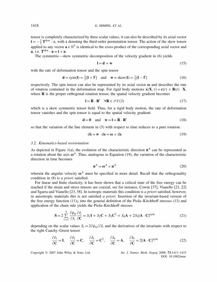
Figure 7. Discretization, loads and boundary conditions of the transversely isotropic tube. A constantsinusoidal displacement load is applied in radial direction at the inside of the tube, with a maximumdisplacement umax

r = 0.3 in the middle of the tube. The upper and lower boundaries of the tube arecompletely fixed. The inclination angle of the characteristic direction is 60◦.

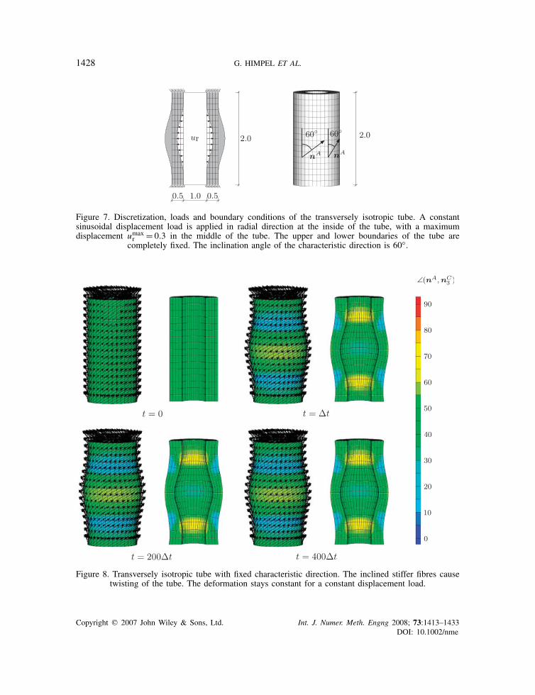
Figure 8. Transversely isotropic tube with fixed characteristic direction. The inclined stiffer fibres causetwisting of the tube. The deformation stays constant for a constant displacement load.



Figure 9. Transversely isotropic tube with fibre reorientation. In the first step, the inclined fi-bres cause twisting of the tube. The fibres reorient along the maximum principal stretch directions.

The reorientation process occurs faster at the begining than towards the final equilibrium state.

fixed in space. The characteristic direction is arranged in the tangential plane with an inclinationangle of 60◦. The material parameters are E = 3.0N/mm2 and = 0.4, related to �= 4.285N/mm2

and �= 1.071N/mm2, as well as �= 2.0N/mm and for reorientation t�= 10.0. The time step isset to �t = 0.1. Once more, fixed characteristic directions are compared with reorientation results.



As one can see in Figure 8, for fixed fibres, the tube twists at the first time step due to higherstiffness of the fibres. The angle between the characteristic direction and the maximum principalstretch direction is distributed inhomogeneously. According to expectations, for a fixed load level,the characteristic direction as well as the deformation stay constant. In Figure 9, the deformationand the fibre directions for reorientation are depicted. For the first time step, as expected, thedeformation and fibre distribution is similar to the case with fixed fibres. For the following timesteps, however, the fibres begin to rotate until they are aligned with the maximum principal stretchdirection. Again, the reorientation proceeds faster at the beginning than close to the final equilib-rium state. The maximum principal stretch direction is tangential in the middle of the tube andaxial at the upper and lower boundary of the tube. As one can see in Figure 9 for 400 time steps,the final fibre distribution is aligned with the principal stretch direction, which is directed axiallyin the upper and lower parts and tangentially in the middle part. Apparent non-symmetries occurdue to the fact that solely the orientation and not the direction governs the material behaviour. Thetwist of the tube, indicated at the beginning of the deformation, recedes due to the reorientationof the fibres.

6. CONCLUSION

The main concern of this contribution is the numerical implementation of fibre reorientationprocesses. For anisotropic elasticity, the free energy reaches a critical state for coaxial stresses andstrains. For transverse isotropy such a coaxiality can be achieved if the structural tensor and thestrain tensor are coaxial. Accordingly, we postulate a reorientation of fibres along the maximumprincipal stretch directions. The incorporation of other criteria, such as for instance, reorientationalong principal stresses or averaged directions, is straightforward and would require only minormodifications of the numerical treatment. Since related algorithms and issues of implementationfollow by analogy for those cases, here we focused exclusively on the strain-driven reorientation.The implementation has been realized by an implicit exponential map for the characteristic directionand application of the Rodriguez formula. Consistent linearizations have been demonstrated onthe local reorientation level as well as on the global finite element level. The theory has beendiscussed by numerical examples. After a demonstration of the general material behaviour interms of a simple tension test, a deformation with a homogeneous as well as an inhomogeneousfinal state has been considered within a finite element setting, wherein we compared materialswith fixed and reorienting fibre directions. In contrast to existing explicit remodelling algorithmssuggested in the literature, the formulation proposed in this contribution is particularly efficient androbust since it relies on consistent algorithmic linearizations both on the local and on the globallevel. Moreover, the suggested computational scheme will not only be useful for the modellingof biological tissue adaptation but rather can also be applied for applications in the wide field ofoptimization processes in material and structural designs.

APPENDIX A: DERIVATIVE OF THE EXPONENT OF A SKEW SYMMETRIC TENSOR

The derivative of the exponent of a skew symmetric tensor v can be determined by application ofthe Rodriguez formula

exp(v)= cos(v)I+ [1− cos(v)]n⊗n+ sin(v)n (A1)



with the norm v=‖v‖, and the normal vector n= v/‖v‖ of the axial vector v=− 12 v

A : e, aswell as the corresponding skew symmetric tensor n=−e · n. Based on this and by making useof index notation, the derivative of the exponent of a skew symmetric tensor with respect to thecorresponding axial vector is

� exp(vi j )�vk

=− sin(v)�i j nk + 1− cos(v)

v[�ikn j + � jkni ] − sin(v)

v�i jk

+[sin(v)− 2

1− cos(v)

v

]nin jnk +

[sin(v)

v− cos(v)

]�i jlnlnk (A2)

Since this derivative includes terms depending on the inverse of the norm of the axial vector, thelimit must be determined by means of l’Hospital’s rule when the norm of the axial vector tendsto zero

limv→0

� exp(vi j )�vk

=−�i jk (A3)

APPENDIX B: DERIVATIVE OF THE EIGENVECTOR WITH RESPECTTO THE CORRESPONDING TENSOR

The eigenvalue problem of the symmetric second-order tensor C∈R3×3

[C− �CI] · nC = 0 (B1)

yields the eigenvalues �CI=1,2,3 ∈R and the eigenvectors nCI=1,2,3 ∈R3 of C. To obtain the derivativeof the eigenvector nCI with respect to the tensorC itself, we follow the lines of derivation highlightedin Mosler and Meschke [44] and combine the derivative of the eigenvalue problem (B1) with respectto the individual component C��[

�C�C��

− ��CI�C��

I

]· nCI + [C− �CI I] ·

�nCI�C��

= 0 (B2)

with the derivative of the constraint that nCI is a normal vector with respect to C��

nCI · nCI = 1 ⇒ nCI ·�nCI�C��

= 0 (B3)

in a linear system of equations

[C− �CI I −nCI

nCIt

0

]︸︷︷︸

K

·

⎡⎢⎢⎢⎢⎣

�nCI�C��

��CI�C��

⎤⎥⎥⎥⎥⎦=

⎡⎢⎣−

�C�C��

· nCI0

⎤⎥⎦ (B4)

The derivative of the eigenvector with respect to one individual component C�� can be obtained bysolving this linear system of Equations (B4) for the vector [[�nCI /�C��]t, ��CI /�C��]t, for instance,



by inverting K. Application of this procedure to each component of the tensor C generates ninevectors �nCI /�C�� ∈R3, which can be combined in the quantity �nCI /�C∈R3×3×3.

For identical eigenvalues �CI ofC the matrixK becomes singular. In that case, small perturbations�� 1 can be applied to the eigenvalues

IF|�A − �B |

max(|�A|, |�B |, |�C |)<tol� THEN

⎧⎪⎨⎪⎩

�A= �A[1+ �]�B = �B[1− �]�C = �C/[[1+ �][1− �]]

(B5)

See, for instance, Miehe [46].

REFERENCES

1. Driessen JBN, Boerboom RA, Huyghe JM, Bouten CVC, Baaijens FPT. Computational analyses of mechanicallyinduced collagen fiber remodeling in the aortic heart valve. Journal of Biomechanical Engineering 2003; 125:549–557.

2. Driessen NJB, Bouten CVC, Baaijens FPT. Improved prediction of the collagen fiber architecture in the aorticheart valve. Journal of Biomechanical Engineering 2005; 127:329–336.

3. Driessen NJB, Peters GWM, Huyghe JM, Bouten CVC, Baaijens FPT. Remodelling of continuously distributedcollagen fibres in soft connective tissues. Journal of Biomechanics 2003; 36:1151–1158.

4. Driessen NJB, Wilson W, Bouten CVC, Baaijens FPT. A computational model for collagen fibre remodelling inthe arterial wall. Journal of Theoretical Biology 2004; 226:53–64.

5. Kuhl E, Garikipati K, Arruda EM, Grosh K. Remodeling of biological tissue: mechanically induced reorientationof a transversely isotropic chain network. Journal of the Mechanics and Physics of Solids 2005; 53:1552–1573.

6. Menzel A. Modelling of anisotropic growth in biological tissues—a new approach and computational aspects.Biomechanics and Modeling in Mechanobiology 2005; 3(3):147–171.

7. Hariton I, deBotton G, Gasser TC, Holzapfel GA. Stress-driven collagen fiber remodeling in arterial walls.Biomechanics and Modeling in Mechanobiology 2007; 6(3):163–175.

8. Imatani S, Maugin GA. A constitutive model for material growth and its application to three-dimensional finiteelement analysis. Mechanics Research Communications 2002; 29:477–483.

9. Menzel A. Anisotropic remodelling of biological tissues. In Mechanics of Biological Tissue, Holzapfel GA,Ogden RW (eds); IUTAM Symposium. Springer: Berlin, 2006; 91–104.

10. Collings PJ. Liquid Crystals: Nature’s Delicate Phase of Matter. Princeton University Press: Princeton, NJ, 1990.11. Ericksen JL. Introduction to the Thermodynamics of Solids (1st edn). Chapman & Hall: London, 1991; 128–150.12. Kamlah M. Ferroelectric and ferroelastic piezoceramics—modeling of electromechanical hysteresis phenomena.

Continuum Mechanics and Thermodynamics 2001; 13:219–268.13. Smith RC. Smart Material Systems. SIAM: Philadelphia, PA, 2005.14. Schroder J, Romanowski H. A thermodynamically consistent mesoscopic model for transversely isotropic

ferroelectric ceramics in a coordinate-invariant setting. Archive of Applied Mechanics 2005; 74:863–877.15. Arockiarajan A, Delibas B, Menzel A, Seemann W. Studies on rate-dependent switching effects of piezoelectric

materials using a finite element model. Computational Materials Science 2006; 37:306–317.16. Arockiarajan A, Menzel A, Delibas B, Seemann W. Computational modeling of rate-dependent domain switching

in piezoelectric materials. European Journal of Mechanics – A/Solids 2006; 25(6):950–964.17. Arockiarajan A, Menzel A, Delibas B, Seemann W. Micromechanical modeling of switching effects in piezoelectric

materials—a robust coupled finite element approach. Journal of Intelligent Material Systems and Structures 2006.DOI 10.1177/1045389x06074117

18. Johansson G, Menzel A, Runesson K. Modeling of anisotropic inelasticity in pearlitic steel at large strains dueto deformation induced substructure evolution. European Journal of Mechanics – A/Solids 2005; 24(6):899–918.

19. Kocks UF, Tome CN, Wenk H-R (eds). Texture and Anisotropy—Preferred Orientations in Polycrystals and theirEffect on Material Properties. Cambridge University Press: Cambridge, 2000.

20. Pedersen NL. On design of fiber-nets and orientation for eigenfrequency optimization of plates. ComputationalMechanics 2006; 39(1):1–13.



21. Vianello M. Coaxiality of strain and stress in anisotropic linear elasticity. Journal of Elasticity 1996; 42:283–289.22. Vianello M. Optimization of the stored energy and coaxiality of strain and stress in finite elasticity. Journal of

Elasticity 1996; 44:193–202.23. Sgarra C, Vianello M. Directions of coaxiality between pure strain and stress in linear elasticicty. Journal of

Elasticity 1997; 46:263–265.24. Chadwick P. Continuum Mechanics. Concise Theory and Problems. Allen & Unwin Ltd: London, 1976.25. Holzapfel GA. Nonlinear Solid Mechanics, A Continuum Approach for Engineering. Wiley: New York, 2000.26. Borchardt-Ott W. Kristallographie. Springer: Berlin, 1997.27. Lokhin VV, Sedov LI. Nonlinear tensor functions of several tensor arguments. Journal of Applied Mathematics

and Mechanics 1963; 27(3):393–417.28. Boehler JP. A simple derivation of representations for non-polynomial constitutive equations in some cases of

anisotropy. Zeitschrift fur Angewandte Mathematik und Mechanik 1979; 59:157–167.29. Spencer AJM. Theory of invariants. In Continuum Physics, Eringen C (ed.), vol. 1. Academic Press: New York,

1971.30. Schroder J. Theoretische und algorithmische Konzepte zur phanomenologischen Beschreibung anisotropen

Materialverhaltens. Ph.D. Thesis, Institut fur Mechanik und Numerische Mechanik, Universitat Hannover,Hannover, 1996.

31. Garikipati K, Olberding JE, Narayanan H, Arruda EM, Grosh K, Calve S. Biological remodelling: stationaryenergy, configurational change, internal variables and dissipation. Journal of the Mechanics and Physics of Solids2006; 54:1493–1515.

32. Epstein M, Maugin GA. Thermomechanics of volumetric growth in uniform bodies. International Journal ofPlasticity 2000; 16:951–978.

33. Kuhl E, Steinmann P. On spatial and material settings of thermo-hyperelastodynamics for open systems. ActaMechanica 2003; 160:179–217.

34. Kuhl E, Steinmann P. Theory and numerics of geometrically nonlinear open system mechanics. InternationalJournal for Numerical Methods in Engineering 2003; 58:1593–1615.

35. Himpel G. On the Modeling of Material Growth in Anisotropic Solids. Internal Variable Approach and NumericalImplementation. Diplomarbeit, Institut fur Mechanik (Bauwesen), Lehrstuhl I, Universitat Stuttgart, 2003.

36. Menzel A, Steinmann P. A view on anisotropic finite hyperelasticity. European Journal of Mechanics – A/Solids2003; 22(1):71–87.

37. Cowin SC. Optimization of the strain energy density in linear anisotropic elasticity. Journal of Elasticity 1994;34:45–68.

38. Sgarra C, Vianello M. Rotations which make strain and stress coaxial. Journal of Elasticity 1997; 47:217–224.39. Betsch P, Menzel A, Stein E. On the parametrisation of finite rotations in computational mechanics—a classification

of concepts with application to smooth shells. Computer Methods in Applied Mechanics and Engineering 1998;155:273–305.

40. Driessen NJB, Cox MAJ, Bouten CVC, Baaijens FPT. Remodelling of the angular collagen fiber distribution incardiovascular tissues. Biomechanics and Modeling in Mechanobiology 2007. DOI 10.1007/s10237-007-0078-x

41. Hughes TJR, Winget J. Finite rotation effects in numerical integration of rate constitutive equations arising inlarge-deformation analysis. International Journal for Numerical Methods in Engineering 1980; 15:1862–1867.

42. Marsden JE, Ratiu TS. Introduction to Mechanics and Symmetry. Springer: Berlin, 1994.43. Gurtin ME. An Introduction to Continuum Mechanics. Mathematics in Science and Engineering, vol. 158.

Academic Press: New York, 1981.44. Mosler J, Meschke G. 3D modeling of strong discontinuities in elastoplastic solids: fixed and rotating localization

formulations. International Journal for Numerical Methods in Engineering 2003; 57:1553–1576.45. Schroder J, Neff P. Invariant formulation of hyperelastic transverse isotropy based on polyconvex free energy

functions. International Journal of Solids and Structures 2003; 40:401–445.46. Miehe C. Computation of isotropic tensor functions. Communications in Numerical Methods in Engineering

1993; 9(11):889–896.


time …biomechanics.stanford.edu/paper/ijnme08a.pdf ·...

Documents