an illustration of the equivalence of the loss of ...biomechanics.stanford.edu/paper/ejmsol06.pdfan...

European Journal of Mechanics A/Solids 25 (2006) 199–214

An illustration of the equivalence of the loss of ellipticity conditionsin spatial and material settings of hyperelasticity

Ellen Kuhl a, Harm Askes b, Paul Steinmann a,∗

a University of Kaiserslautern, Faculty of Mechanical Engineering, P.O. Box 3049, D-67653 Kaiserslautern, Germanyb Department of Civil and Structural Engineering, University of Sheffield, Sheffield S1 3JD, United Kingdom

Received 24 June 2004; accepted 29 July 2005

Available online 20 October 2005

Abstract

The loss of ellipticity indicated through the rank-one-convexity condition is elaborated for the spatial and material motionproblem of continuum mechanics. While the spatial motion problem is characterized through the classical equilibrium equationsparametrised in terms of the deformation gradient, the material motion problem is driven by the inverse deformation gradient. Assuch, it deals with material forces of configurational mechanics that are energetically conjugated to variations of material place-ments at fixed spatial points. The duality between the two problems is highlighted in terms of balance laws, linearizations includingthe consistent tangent operators, and the acoustic tensors. Issues of rank-one-convexity are discussed in both settings. In particu-lar, it is demonstrated that if the rank-one-convexity condition is violated, the loss of well-posedness of the governing equationsoccurs simultaneously in the spatial and in the material motion context. Thus, the material motion problem, i.e. the configurationalforce balance, does not lead to additional requirements to ensure ellipticity. This duality of the spatial and the material motionapproach is illustrated for the hyperelastic case in general and exemplified analytically and numerically for a hyperelastic materialof Neo-Hookean type. Special emphasis is dedicated to the geometrical representation of the ellipticity condition in both settings. 2005 Elsevier SAS. All rights reserved.

Keywords: Loss of ellipticity; Rank-one-convexity; Localization; Configurational mechanics; Spatial and material settings

1. Introduction

Continuum motion can be described via a Lagrangian or a Eulerian description. In the former, material particles arefollowed in space, whereas in the latter, material flow along fixed spatial positions is tracked. This is closely relatedto spatial and material settings of continuum mechanics. In the spatial setting, spatial (or physical) forces are dealtwith that are energetically conjugated to spatial variations of fixed material points. This is the viewpoint of classical,Newtonian mechanics. Conversely, in the material setting, material (or configurational) forces are encountered thatare energetically conjugated to material variations at fixed spatial positions. The latter formalism is also known asthe viewpoint due to Eshelby, see Eshelby (1951, 1975). The material setting of continuum mechanics or rather

* Corresponding author.E-mail addresses: [email protected] (E. Kuhl), [email protected] (H. Askes), [email protected] (P. Steinmann).URL: http://mechanik.mv.uni-kl.de (P. Steinmann).

0997-7538/$ – see front matter 2005 Elsevier SAS. All rights reserved.doi:10.1016/j.euromechsol.2005.07.008

200 E. Kuhl et al. / European Journal of Mechanics A/Solids 25 (2006) 199–214

configurational mechanics has received considerable attention in recent years, cf. Chadwick (1975), Maugin andTrimarco (1992), Maugin (1999a, 1999b), Gurtin (1995), Gurtin and Podio-Guidugli (1996), Dascalu and Maugin(1995), Silhavý (1997), Kienzler and Herrmann (2000), Podio-Guidugli (2002) or the extended monographs (Maugin,1993, 1995; Gurtin, 2000). In particular, the duality between the spatial and the material setting is elucidated forvarious cases and applications in Maugin (1993), Steinmann (2002a, 2002b, 2002c), Kuhl and Steinmann (2003).

In the context of configurational mechanics, material force residuals arise as a result of inhomogeneities. Thus, thestudy of the material motion problem is relevant for problems involving propagating discontinuities such as cracks,voids and inclusions. Especially when the two problems, i.e. spatial motion and material motion, are studied in parallel,it is enlighting to analyse the ellipticity of either problem, see e.g. Ball (1977a, 1977b). In the infinitesimal context,the convexity condition is strongly related to the classical criterion of uniqueness in terms of the positive definitenessof the second order work (Drucker, 1950; Hill, 1958). The general convexity condition, however, is typically toorestrictive from a physical point of view and moreover too difficult to evaluate from a mathematical point of view.A weaker condition, yet having a well-established mathematical status is the condition of rank-one-convexity. In theinfinitesimal sense, rank-one-convexity corresponds to the classical Legendre–Hadamard condition which dates backto the early work of Hadamard on the propagation of waves, see e.g. Hadamard (1903), Hill (1958, 1962), Truesdelland Noll (1965), Ogden (1984). For the class of non-transient problems considered herein, the loss of rank-one-convexity is one-to-one related to the loss of ellipticity which is typically accompanied by the loss of well-posednessof the governing equations. The elaboration of the ellipticity condition is thus of fundamental interest, not only for thespatial but also for the material motion problem.

Although the notions of convexity, uniqueness, monotony, stability, rank-one-convexity, ellipticity and well-posedness are well-established in the spatial motion context, see e.g. Rice (1976), Rice and Rudnicki (1980), Benallal(1992), Benallal and Comi (1996), Benallal and Bigoni (2004), Bigoni (2000), Petryk (1992, 2000) amongst others,the appropriate classification within what we shall call the material motion context has not been considered to thesame extend. As an exception the relations between the spatial and material motion convexity and rank-one-convexitycondition have been elaborated in a completely different spirit within the framework of functional analysis in Ball(1977b). Here we want to illustrate those rather abstract results within the spatial and material settings of hyperelas-ticity in order to highlight the connection of these fundamental results to the notion of configurational mechanics.In particular, a difference between the two settings in this respect would be significant, for instance if the materialmotion problem would lose ellipticity or rather rank-one-convexity at an earlier stage of loading than the spatial mo-tion problem, or vice versa. Recall, that aspects of uniqueness, monotony or convexity can either be studied on theglobal/structural level or on the local/constitutive level. Within this study, we restrict ourselves to the constitutivelevel.

After reiterating the governing equations in both settings in Section 2, relevant tangent operators are derivedthrough a consistent linearisation of both problems in Section 3. Next, in Section 4, we elaborate the issue of elliptic-ity which can be expressed in terms of the acoustic tensors. For illustration purposes, the corresponding localisationanalysis is exemplified in Section 5 for a Neo-Hookean material, whereby the eigenvalues of both acoustic tensors areanalysed. Finally, some conclusions will be drawn in Section 6. For the sake of completeness, we shall reiterate theclassical Legendre–Hadamard condition in Appendix A.

2. Governing equations

To set the stage, let us briefly summarise the relevant kinematic relations, the underlying variational principle andits linearisation and the corresponding stress measures of the spatial and the material motion problem.

2.1. Spatial motion problem

The familiar spatial motion problem is characterised through the nonlinear spatial deformation map x =ϕ(X, t) :B0 → Bt mapping placements from the material configuration B0 to the spatial configuration Bt . The cor-responding linear tangent map from the material tangent space TB0 to the spatial tangent space TBt can then beexpressed in terms of the spatial motion deformation gradient F = ∇Xϕ(X, t) :TB0 → TBt and its determinantJ = detF > 0 which is required to be strictly positive. Moreover, the right and left spatial motion Cauchy–Greenstrain tensors C = F t · F and b = F · F t can be introduced as typical strain measures of the spatial motion problem.

E. Kuhl et al. / European Journal of Mechanics A/Solids 25 (2006) 199–214 201

Recall that C can be interpreted as the pull back of the covariant spatial metric whereas b is the push forward of thecontravariant material metric. In what follows, we shall restrict ourselves to hyperelastic conservative systems whichcan essentially be characterised through a variational principle of Dirichlet type. We thus introduce the internal po-tential energies W0 and Wt , in this case the strain energy densities per unit volume in B0 and Bt , respectively. For thesake of simplicity, we shall assume that the external potential energy vanishes identically such that the total energy Ican be introduced as the integral of either of the strain energies density over the corresponding domain.

I(ϕ) =∫

B0

W0 dV0 =∫

Bt

Wt dVt → stat. (1)

Its stationary point obviously corresponds to a vanishing variation of the total energy density I with respect to thespatial deformation ϕ.

δϕI(ϕ) =∫

B0

∇Xδϕ : DF W0 dV0 =∫

Bt

∇xδϕ : [WtI − f t · df Wt ]dVt = 0. (2)

Herein, f denotes the deformation gradient of the material motion problem, which will be discussed in detail later inthe following subsection. Moreover, we could formally introduce the linearisation of the above spatial variation δϕIwith respect to the spatial motion deformation ϕ.

∆ϕδϕI(ϕ) =∫

B0

∇Xδϕ : D2FF W0 : ∇X∆ϕ dV0. (3)

The particular format of Eq. (2) motivates the introduction of the spatial motion stresses Πt and σ t = jΠt · F t,

Πt = DF W0, σ t = WtI − f t · df Wt (4)

whereby the former denotes the classical two-point Piola stress tensor while the latter is typically referred to as Cauchystress. With these abbreviations at hand, the familiar Euler–Lagrange field equations of the spatial motion problem

divX Πt = 0, divx σ t = 0 (5)

follow directly form the evaluation of the spatial variation of the total potential energy (2). For further reference, itproves convenient to additionally introduce the following stress tensors.

τ t = Πt · F t, M t = F t · Πt, Y t = F t · Πt · F t. (6)

Hereby, τ t = Jσ t denotes the Kirchhoff stress tensor which is typically given in spatial description, M t is the classicalMandel stress tensor in material description and Y t is another two-point stress tensor of the spatial motion problem.

2.2. Material motion problem

The material motion problem is the appropriate setting of configurational mechanics. Thereby, in analogy to thespatial motion map ϕ, we could introduce a material motion map X = Φ(x, t) :Bt → B0 which essentially defines themapping of placements from the spatial configuration Bt to the material configuration B0. Accordingly, the materialmotion deformation gradient f = ∇xΦ(x, t) :TBt → TB0 defines the linear tangent map from the spatial tangentspace TBt to the material tangent space TB0, whereby j = detf > 0 denotes the corresponding Jacobian. Moreover,we introduce the right and left material motion Cauchy–Green strain tensors c = f t · f and B = f · f t which canbe interpreted as the push forward of the covariant material metric and as the pull back of the contravariant spatialmetric, respectively. In the case of configurational equilibrium, the Euler–Lagrange equations of the material motionproblem follow from the appropriate evaluation of the related Dirichlet principle in terms of the stationarity of thetotal energy I , however, now parametrised in terms of the material motion map Φ .

I(Φ) =∫

Wt dVt =∫

W0 dV0 → stat. (7)

Bt B0


Accordingly, for the material motion problem, the minimum of the total energy density I corresponds to a vanishingvariation with respect to the material deformation Φ .

δΦI(Φ) =∫

Bt

∇xδΦ : df Wt dVt =∫

B0

∇XδΦ : [W0I − F t · DF W0]dV0 = 0. (8)

Again, we could formally introduce the linearisation of the material variation δΦI with respect to the material defor-mation Φ .

∆ΦδΦI(Φ) =∫

Bt

∇xδΦ : d2f f Wt : ∇x∆Φ dVt . (9)

Next, we introduce the material motion stresses π t and Σ t = Jπ t · f t,

π t = df Wt, Σ t = W0I − F t · DF W0 (10)

the former denoting a two-point stress tensor of Piola type and the latter being the classical Eshelby stress, a stresstensor in material description. Accordingly, the Euler–Lagrange field equations of the material motion problem whichfollow straightforwardly from Eq. (8)

divxπ t = 0, divX Σ t = 0 (11)

take a formally dual structure to the Euler–Lagrange equations of the spatial motion problem, compare Eqs. (5).Moreover, it proves convenient to introduce the following stress tensors of the material motion problem,

T t = π t · f t, mt = f t · π t, yt = f t · π t · f t (12)

whereby T t = jΣ t denotes a stress measure of Kirchhoff type in material description, mt is typically addressed asthe stress tensor of the chemical potential in spatial description and yt denotes another two-point stress of the materialmotion problem.

2.3. Spatial vs. material motion stresses

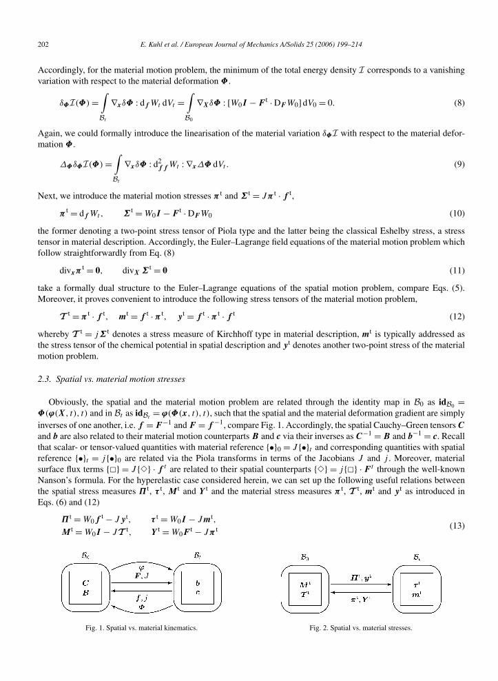
Obviously, the spatial and the material motion problem are related through the identity map in B0 as idB0 =Φ(ϕ(X, t), t) and in Bt as idBt

= ϕ(Φ(x, t), t), such that the spatial and the material deformation gradient are simplyinverses of one another, i.e. f = F−1 and F = f −1, compare Fig. 1. Accordingly, the spatial Cauchy–Green tensors C

and b are also related to their material motion counterparts B and c via their inverses as C−1 = B and b−1 = c. Recallthat scalar- or tensor-valued quantities with material reference •0 = J •t and corresponding quantities with spatialreference •t = j•0 are related via the Piola transforms in terms of the Jacobians J and j . Moreover, materialsurface flux terms = J · f t are related to their spatial counterparts = j · F t through the well-knownNanson’s formula. For the hyperelastic case considered herein, we can set up the following useful relations betweenthe spatial stress measures Πt, τ t, M t and Y t and the material stress measures π t, T t, mt and yt as introduced inEqs. (6) and (12)

Πt = W0ft − Jyt, τ t = W0I − Jmt,

M t = W0I − JT t, Y t = W0Ft − Jπ t (13)

Fig. 1. Spatial vs. material kinematics. Fig. 2. Spatial vs. material stresses.


and vice versa

π t = WtFt − jY t, T t = WtI − jM t,

mt = WtI − jτ t, yt = Wtft − jΠt (14)

by making use of the definitions given in Eqs. (4) and (10), compare Fig. 2.

3. Linearization

The present section is dedicated to the appropriate linearization of the stress strain relations of both, the spatialand the material motion problem. They lend themselves to the introduction or several fourth order tangent operators.Useful relations between spatial and material motion tangent operators will be derived.


The fourth order tensor A denotes the familiar spatial motion tangent operator in two-point description, i.e. thesecond derivative of the internal potential energy density W0 with respect to the spatial motion deformation gradientF as introduced earlier in Eq. (3).

A = D2FF W0 = DF Πt. (15)

For a particular free energy function W0, e.g. the hyperelastic Neo-Hookean free energy to be elaborated in Section 5,we can express the tangent operator A in terms of the derivatives of the Jacobians J and j

DF J = Jf t, DF j = −jf t (16)

and of the derivatives of the deformation gradients F and f

DF F = I ⊗I , DF F t = I ⊗ I , DF f = −f ⊗f t, DF f t = −f t ⊗f (17)

with respect to the spatial motion deformation gradient F itself. In the above equations, we have introduced theabbreviations [•⊗]ijkl = [•]ik ⊗ []jl and [•⊗]ijkl = [•]il ⊗ []jk for the non-standard dyadic products of twosecond order tensors. With these considerations at hand, we can straightforwardly introduce the pull back and pushforward of the two-point tensor A. To this end, we make use of the following operation

[•t ⊗] : A : [•⊗t] with [•], [] ∈ I ,F (18)

whereby the choice of first tensor [•] = F corresponds to a covariant pull back of the first and third index of A and[] = F denotes a contravariant push forward of the second and fourth index. Obviously, for [•] = I and [] = I thecorresponding indices remain unaffected. With the above considerations, we can easily generate the pull back andpush forward of the spatial motion tangent operator A.

b = [I t ⊗F ] : A : [I ⊗F t],C = [F t ⊗I ] : A : [F ⊗I t],d = [F t ⊗F ] : A : [F ⊗F t].

(19)

Accordingly, the fourth order tensor b is expressed in the spatial description similar to the left Cauchy–Green straintensor b while the fourth order tensor C is denoted in the material description according to the right Cauchy–Greenstrain tensor C. The fourth order tangent operator d is denoted in the two-point description, however, with pairwiseopposite indices compared to A, compare Fig. 3.

Fig. 3. Spatial vs. material tangent operators.



The, to our knowledge up to now never considered, fourth order tangent operator a of the configurational problemis a tensor in two-point description, characterising the second derivative of the internal potential energy density Wt

with respect to the material motion deformation gradient f which was introduced earlier in Eq. (9).

a = d2f f Wt = df π t. (20)

In Section 5, we will evaluate the above equation for a particular hyperelastic free energy function Wt(f ) of Neo-Hooke type. To this end, we will require the derivatives of the Jacobians j and J

df j = jF t, df J = −JF t (21)

and of the deformation gradients f and F

df f = I ⊗I , df f t = I ⊗ I , df F = −F ⊗F t, df F t = −F t ⊗F (22)

with respect to the material motion deformation gradient f . Based on these preliminary considerations, we can intro-duce the following push forward and pull back operations

[•t ⊗] : a : [•⊗t] with [•], [] ∈ I ,f (23)

whereby now [•] = f denotes the covariant push forward of the first and third index of a and [] = f indicates thecontravariant pull back of its second and fourth index, respectively. Again, the identity maps [•] = I and [] = I donot change the corresponding index. We thus introduce the following abbreviations for the material motion tangentoperators,

B = [I t ⊗f ] : a : [I ⊗f t],c = [f t ⊗I ] : a : [f ⊗I t],D = [f t ⊗f ] : a : [f ⊗f t]

(24)

whereby B is obviously a fourth order tensor in material description, c is denoted in spatial description and D is atensor in two-point description similar to the spatial motion tangent operator A with pairwise opposite indices as a.

3.3. Spatial vs. material tangent operators

In the previous section, we have set up relations between the different spatial and material stress measures. Bymaking use of Eqs. (13) and (14) in particular, we can rewrite the spatial motion tangent operator A in terms of thematerial stress π t whereas the material motion tangent operator a can be expressed in terms of the spatial stress Πt.

A = DF Πt = DF [JWtft − Jf t · π t · f t],

a = df π t = df [jW0Ft − jF t · Πt · F t]. (25)

The thorough evaluation of the above equation renders as a new result the following useful relations between thespatial motion tangent operators A, b, C and d and their material counterparts a, B, c and D

A = Πt ⊗ f t − f t ⊗Π − Πt ⊗f + f t ⊗ Πt − W0ft ⊗ f t + W0f

t ⊗f + JD,

b = τ t ⊗ I − I ⊗τ − τ t ⊗I + I ⊗ τ t − W0I ⊗ I + W0I ⊗ I + Jc,

C = M t ⊗ I − I ⊗M − M t ⊗I + I ⊗ M t − W0I ⊗ I + W0I ⊗ I + JB,

d = Y t ⊗ F t − F t ⊗Y − Y t ⊗F + F t ⊗ Y t − W0Ft ⊗ F t + W0F

t ⊗F + Ja

(26)

and vice versa,

a = π t ⊗ F t − F t ⊗π − π t ⊗F + F t ⊗ π t − WtFt ⊗ F t + WtF

t ⊗F + jd,

B = T t ⊗ I − I ⊗T − T t ⊗ I + I ⊗ T t − WtI ⊗ I + WtI ⊗ I + jC,

c = mt ⊗ I − I ⊗m − mt ⊗I + I ⊗ mt − WtI ⊗ I + WtI ⊗ I + jb,

D = yt ⊗ f t − f t ⊗y − yt ⊗f + f t ⊗ yt − Wtft ⊗ f t + Wtf

t ⊗f + jA

(27)

compare Fig. 3. Recall the practical relevance of the fourth order tangent operators within a Newton–Raphson basedsolution strategy in a finite element scheme. In this context, the tangent operators A and a are of particular importance,see Kuhl et al. (2004) and Askes et al. (2004). Their relevance in the context of rank-one-convexity is illustrated in thefollowing section.


4. Ellipticity

In the previous section, we have introduced the spatial and the material tangent operators A and a. Their positivesemi-definiteness is typically analysed to study the convexity of the underlying motion problem. In what follows, weshall relax the classical condition of convexity to the in some cases less restrictive requirement of rank-one-convexity.Following arguments of duality, we discuss the rank-one-convexity condition or rather ellipticity condition for both thespatial and the material motion problem. By setting up relations between the spatial and the material motion acoustictensor, we will show that both are simply related via weighted pull back/push forward operations. A relation to theclassical Legendre–Hadamard condition in terms of the acoustic tensors is given in Appendix A.


The rank-one-convexity condition of the spatial motion problem can be expressed as follows.

[m ⊗ N] : A : [m ⊗ N] 0. (28)

For [m ⊗ N ] : A : [m ⊗ N] > 0, it ensures that the underlying quasi-static spatial motion problem remains elliptic. Byintroducing the contravariant pull back of the spatial unit tangent m and the covariant push forward of the materialunit normal N as

M = f · m = m · f t, n = f t · N = N · f (29)

we can reformulate the above equation in terms of the four different tangent operators A, b, C and d introduced inEq. (19).

[m ⊗ n] : b : [m ⊗ n] 0,

[M ⊗ N ] : C : [M ⊗ N ] 0,

[M ⊗ n] : d : [M ⊗ n] 0.

(30)

Alternatively, the above equations could be formulated as a requirement of positive semi-definiteness

m · q · m 0, q = [I ⊗ N ] : A · N = [I ⊗ n] : b · n,

M · Q · M 0, Q = [I ⊗ N ] : C · N = [I ⊗ n] : d · n (31)

in terms of the second order tensor q in spatial description and its pull back Q = F t · q · F in material description, acondition which can equivalently be expressed in the following form.

det(q) 0, det(Q) 0. (32)

Because of its connection with the propagation of infinitesimal plane waves, the second order tensor q is called theacoustic tensor of the spatial motion problem. The vector N then represents the direction of wave propagation whichcorresponds to the normal to the discontinuity surface in the quasi-static case while m takes the interpretation of ajump vector.


In complete analogy to the spatial motion problem, in configurational mechanics, the rank-one-convexity conditionof the material motion problem takes the following format.

[M ⊗ n] : a : [M ⊗ n] 0. (33)

For [M ⊗ n] : a : [M ⊗ n] > 0, the above rank-one-convexity condition yields to the condition of ellipticity of thequasi-static material motion problem. With the help of the contravariant push forward of the material tangent M andthe covariant pull back of the spatial normal n

m = F · M = M · F t, N = F t · n = n · F (34)


we can easily generate alternative expressions in terms of the different tangent operators a, B, c and D introduced inEq. (24).

[M ⊗ N ] : B : [M ⊗ N ] 0,

[m ⊗ n] : c : [m ⊗ n] 0,

[m ⊗ N ] : D : [m ⊗ N ] 0.

(35)

A reformulation of the above equations

M · Q · M 0, Q = [I ⊗ n] : a · n = [I ⊗ N] : B · N ,

m · q · m 0, q = [I ⊗ n] : c · n = [I ⊗ N] : D · N (36)

introduces the requirement of positive semi-definiteness of the material motion acoustic tensor Q and its push forwardq = f t · Q · f , whereby their non-negative determinant

det(Q) 0, det(q) 0 (37)

ensures ellipticity of the material motion problem. Again, n characterises the spatial normal to the discontinuitysurface while M denotes the corresponding jump vector.

4.3. Spatial vs. material acoustic tensor

To elaborate the relations between the spatial motion acoustic tensor q = [I ⊗N] : DF Π ·N and its material motioncounterpart Q = [I ⊗ n] : df π · n we shall express DF Π and df π in terms of their dual counterparts according toEqs. (26) and (27).

q = t ⊗ n − n ⊗ t − W0n ⊗ n + W0n ⊗ n − t ⊗ n + n ⊗ t + Jf t · n · df π · n · f ,

Q = T ⊗ N − N ⊗ T − WtN ⊗ N + Wt

N ⊗ N − T ⊗ N + N ⊗ T + jF t · N · DF Π · N · F .(38)

For notational simplicity, we have introduced the spatial and the material traction vector t = Πt · N and T = π t · n,the push forward of the material normal n and the pull back of the spatial normal N . Due to the symmetric structureof the acoustic tensors, all but the last term cancel and we are left with the following remarkably simple expressions.

q = [I ⊗ N ] : DF Π · N = Jf t · [I ⊗ n] : df π · n · f ,

Q = [I ⊗ n] : df π · n = jF t[I ⊗ N] : DF Π · N · F .(39)

The right-hand sides of the above equation can easily be identified as the scaled push forward of the material motionacoustic tensor q and the pull back of the spatial motion acoustic tensor Q introduced in Eqs. (36) and (31), compareFig. 4.

q = Jλ2nq,

Q = jΛ2N

Q withq = f t · Q · f ,

Q = F t · q · F .(40)

Apparently, the spatial motion acoustic tensor q follows straightforwardly from a push forward of its material motioncounterpart Q weighted by the corresponding Jacobian and the square of the related stretch λn = ‖n‖ = √

N · B · N =Λ−1

N and ΛN = ‖N‖ = √n · b · n = λ−1

n . Of course, this result is neither astonishing nor unexpected. The equivalenceof the spatial and material rank-one-convexity condition (28) and (33) has been shown already by Ball in the moreabstract setting of functional analysis, see Ball (1977b). By making use of the change of variables formula, he provedthat Wt(f ) is rank-one-convex if and only if W0(F ) is rank-one-convex without explicitly referring to the implications

Fig. 4. Spatial vs. material acoustic tensors.


Fig. 5. Pure shear with Λ = 2 and ν = 0.45—eigenvalues of spatial motion problem (top) and material motion problem (bottom).

within configurational mechanics. Thus, in summary of our investigations, as the main result it occurs that providedthat the underlying deformation is invertible, i.e. J > 0 and accordingly j > 0, F = f −1 and f = F−1, the loss ofellipticity of the spatial and the material motion problem takes place simultaneously. Accordingly, the determinant ofthe acoustic tensors q and Q

det(q) = 0 ⇔ det(Q) = 0 (41)

vanishes simultaneously for the spatial and the material motion problem.

5. Model problem: Neo-Hookean material

In the remainder of this study, we assume a frequently used strain energy density of the compressible Neo-Hookeantype with

W0 = 1

2λ0 ln2(J ) + 1

2µ0

[C : I − ndim − 2 ln(J )

](42)

for the spatial and

Wt = 1λt ln2(j−1) + 1

µt

[c−1 : I − ndim − 2 ln(j−1)

](43)

2 2


Fig. 6. Simple shear with Λ = 2 and ν = 0.45—eigenvalues of spatial motion problem (top) and material motion problem (bottom).

for the material motion case. Thereby, ndim is the number of spatial dimensions of the problem under consideration andµ0, λ0, µt = jµ0 and λt = jλ0 are the Lamé parameters of the spatial and the material motion problem, respectively.With this particularisation, the tangent operator of the spatial motion problem can be elaborated as

tan A = λ0ft ⊗ f t + µ0I ⊗I + [

µ0 − λ0 ln(J )]f t ⊗f (44)

whereas the much more involved tangent operator of the material motion problem can be written as follows.

tan a = [Wt − 2λt ln(J ) + 2µt + λt

]F t ⊗ F t − [

Wt − λt ln(J ) + µt

]F t ⊗F

+ µt [C · F t ⊗F + F t ⊗F · C − C · F t ⊗ F t − F t ⊗ C · F t + C ⊗b]. (45)

The acoustic tensors that correspond to the spatial and to the material motion problem are obtained by substitutingEqs. (44) and (45) into Eqs. (31) and (36). Although the tangent operators themselves differ considerably for thespatial and the material motion case, the acoustic tensors of the spatial

q = [λ0

[1 − ln(J )

] + µ0]n ⊗ n + µ0I (46)

and the material motion problem

Q = Λ2N

[[λt

[1 − ln(J )

] + µt

]N ⊗ N + µtC

](47)

take a remarkably similar format and are of course related through Eq. (40).


Fig. 7. Uniaxial tension with Λ = 4 and ν = 0.45—eigenvalues of spatial motion problem (top) and material motion problem (bottom)

5.1. Analytical elaboration of rank-one-convexity

Loss of ellipticity or rather loss of rank-one-convexity occurs when the determinant of the acoustic tensor becomeszero. Following Eqs. (46) and (47), the two determinants for the two-dimensional case can be elaborated in Cartesiancoordinates as

det(q) = [λ0µ0

[1 − ln(J )

] + µ20

][[f11c + f21s]2 + [f12c + f22s]2] + µ20 (48)

and

det(Q) = ΛN

[[λtµt

[1 − ln(J )

] + µ2t

][[F11s − F12c]2 + [F21s − F22c]2] + µ2t J

2] (49)

respectively. Herein, we have introduced the short-hand notation c = cos(α) and s = sin(α) in terms of the angle α

defining the material normal as N = [cosα, sinα]t. For a number of fundamental loading cases, we examine whenloss of ellipticity occurs:

• Pure shear is described by taking the deformation gradient equal to F11 = Λ, F22 = 1/Λ and F12 = F21 = 0,hence J = det(F ) = 1. It can be verified that Eqs. (48) and (49) then reduce to a summation of quadratic terms.Therefore, ellipticity is a priori guaranteed throughout.

• Simple shear is invoked via F11 = F22 = 1, F12 = Λ and F21 = 0. The same observations apply as for the case ofpure shear.


Fig. 8. Biaxial tension with Λ = 3 and ν = 0.45—eigenvalues of spatial motion problem (top) and material motion problem (bottom).

• Uniaxial tension can be described by F11 = Λ, F22 = 1 and F12 = F21 = 0. Elaborating either of the two deter-minants given in Eqs. (48) and (49) reveals that ellipticity is lost if λ0[1 − ln(Λ)] + 2µ0 0 whereby the criticaldirection for both determinants is given by α = π/2. From solving the above equation, a critical stretch Λ can bedetermined in terms of the Poisson’s ratio ν. Ellipticity is lost if Λ exp([1 − ν]/ν).

• Biaxial tension is generated by taking F11 = F22 = Λ and F12 = F21 = 0. Ellipticity is lost if the transcendentalinequality λ0[1 − ln(Λ2)] + µ0[1 + Λ2] 0 is satisfied, where again the two determinants give identical results.For values of ν > 0.4464 ellipticity cannot be guaranteed.

As has been argued already in the previous sections: if loss of ellipticity occurs, it occurs concurrently in the spatialmotion problem and in the material motion problem.

5.2. Numerical elaboration of rank-one-convexity

Next, the eigenvalues of the two acoustic tensors are investigated. The same four loading cases are studied as inSection 5.1. Throughout, the elastic constants have been taken as λ0 = 7759 MPa and µ0 = 862 MPa correspondingto E = 2500 MPa and ν = 0.45 in the small strain limit. For the loading cases pure shear and simple shear a stretchΛ = 2 has been taken, we analyse the uniaxial tension case with Λ = 4, and Λ = 3 has been used for the biaxial case.The results are plotted in Figs. 5–8. For the considered loading cases four eigenvalues are non-trivial: two accordingto q and two according to Q. In Figs. 5–8 the eigenvalues are multiplied with the components of N to arrive at a


Fig. 9. Eigenvalues as a function of the stretch Λ for the material motion problem (solid) and the spatial motion problem (dashed) — pure shear(top left), simple shear (top right), uniaxial tension (bottom left) and biaxial tension (bottom right).

two-dimensional visualisation: denoting the eigenvalues by h, we plot h cos(α) on the horizontal axis and h sin(α) onthe vertical axis.

For the cases of pure shear and simple shear, where ellipticity or rather rank-one-convexity is guaranteed for anyvalue of the stretch Λ, the eigenvalues remain always positive. Since the two acoustic tensors q and Q are related viatwo contractions in terms of the (inverse) deformation gradient, the shape of the eigenvalue plots is very similar forthe spatial motion problem as compared to the material motion problem; cf. the top rows and bottom rows in Figs. 5and 6. For instance, the smaller eigenvalue of the spatial motion problem yields a circle with radius µ0 (see Figs. 5and 6, upper left), which translates into lemon-like curves for the material motion problem (Figs. 5 and 6, bottomleft). Similar observations hold for the larger eigenvalue, depicted in the right columns of Figs. 5 and 6. In the lattercurves, the direction of the maximum eigenvalue for the spatial motion problem coincides with the direction of theminimum eigenvalue for the material motion problem, and vice versa. This is due to the fact that if for a certain angleα a maximum value for F is obtained, then a minimum value for f is found, and vice versa.

If uniaxial tension is assumed, a critical stretch exists beyond which the determinants of the acoustic tensorsbecome negative. In Fig. 7 the eigenvalues of both acoustic tensors are plotted for a stretch larger than the criticalstretch. For certain values of α, one of the eigenvalues becomes negative which results in flower-like curves as shownin the left column of Fig. 7. This dependence on α was already used in the derivation of the critical equation λ0[1 −ln(Λ)] + 2µ0 0. The negative eigenvalues appear and develop in similar ways for the spatial motion problem andthe material motion problem. Again, in the spatial motion problem one of the eigenvalues adopts the (non-negative)


constant value µ0, which is transformed into a (non-negative) eigenvalue for the material motion problem via twocontractions with the deformation gradient (cf. right column of Fig. 7).

Finally, loss of ellipticity, i.e. rank-one-convexity, can also occur in case of biaxial tension. In contrast to uniaxialtension, loss of rank-one-convexity does not depend on the angle α. This is reflected in the circles plotted in Fig. 8. Theleft column of Fig. 8 consists of eigenvalues that are all negative, the right column contains only positive eigenvalues.The radii of the circles described by the material motion problem are related to the radii of the circles from the spatialmotion problem via a factor Λ2. According to Eq. (40), the two acoustic tensors relate as Q = jΛ2

NF t · q ·F . For thisspecific loading case with F = ΛI and j = Λ−2, the above equation simplifies to Q = Λ2q , compare also Eqs. (46)and (47).

In Fig. 9 the evolution of the minimum eigenvalues of q and Q is plotted as a function of the stretch Λ. Note thatthese minimum values do not necessarily correspond to a single orientation α during the entire loading process. It isagain seen that the eigenvalues for the loading cases pure shear and simple shear are always positive, and that one ofthe eigenvalues of the spatial motion problem is constant and equal to the Lamé constant µ0. For the loading casesuniaxial tension and biaxial tension one of the two eigenvalues for either problem (spatial motion problem or materialmotion problem) may become negative. The critical values of Λ for which this occurs have been derived analyticallyin Section 5.1; here, it is confirmed numerically that negative eigenvalues appear simultaneously in the spatial motionproblem and the material motion problem.

6. Conclusions

In this paper, we have considered the conditions for ellipticity or rather rank-one-convexity for the common spatialand the material motion problem of configurational mechanics. The governing equations, linearizations and acoustictensors for the two problems have been presented in a completely dual format. As a consequence from the classicalfar-reaching result by Ball (1977a) it turns out that the acoustic tensors associated with the two problems can beretrieved from one another via straightforward push forward/pull back operations. Loss of ellipticity or rather rank-one-convexity clearly occurs simultaneously in the spatial and in the material motion problem although the mechanicalinterpretation of these two problems is quite different. In other words, studying the material motion problem or ratherthe problems of configurational mechanics does not lead to additional difficulties: as long as the spatial motion prob-lem remains well-posed, the material motion problem will not become ill–posed due to the loss of rank-one-convexity.

This has been illustrated for a hyperelastic sample material with a compressible Neo-Hookean strain energy density.Four fundamental loading cases have been investigated, both analytically and numerically: if negative eigenvaluesoccur, they appear concurrently in the acoustic tensors of the two problems.

Appendix A. Spatial and material Legendre–Hadamard condition

For the sake of completeness, we shall briefly summarize the traditional derivation of the Legendre–Hadamardcondition as illustrated in Hadamard (1903), Thomas (1961) and Hill (1962). Its derivations are based on the kinematiccompatibility conditions for a first order discontinuity surface

DtF = ωm ⊗ N , dtf = ΩM ⊗ n (A.1)

which are also referred to as Maxwell’s compatibility conditions (Maxwell, 1873). Therein, N and n represent thematerial and the spatial normal to the discontinuity surface, M and m are the corresponding jump vectors and Ω andω denote the magnitude of the jump as illustrated in Fig. A.1. The evaluation of Cauchy’s lemma in combination withCauchy’s theorem then renders the equilibrium equations across a singular surface,

DtΠt · N = 0, dtπ

t · n = 0 (A.2)

whereby •= [•]+ −[•]− denotes the jump of the quantity [•] across the singular surface. Together with incrementalconstitutive equation for a hyperelastic material for the spatial DtΠ

t = A : DtF and the material motion problemdtπ

t = a : dtf the equilibrium equations (A.2) can be reformulated as follows.

A : DtF · N = 0, a : dtf · n = 0. (A.3)


Fig. A.1. Spatial vs. material kinematics of singular surfaces.

Last, we make use of Hill’s assumption of a linear comparison solid (Hill, 1958), i.e. A= 0 and a= 0, respectively,to end up with alternative representations of Eqs. (28) and (33).[

A : [ωm ⊗ N]] · N = 0,[a : [ΩM ⊗ n]] · n = 0. (A.4)

These can be recast into the corresponding special eigenvalue problems q · m = 0 and Q · M = 0 in terms of theacoustic tensors of the spatial and the material motion problem q = [I ⊗ N] : DF Π · N and Q = [I ⊗ n] : df π · n.For the non-transient case considered herein, the vanishing determinant of the acoustic tensors

det(q) = 0, det(Q) = 0 (A.5)

indicates the loss of ellipticity of the spatial and the material motion problem which manifests itself in the formationof rank-one-laminates. The angles θ and Θ

cos(θ) = m · n, cos(Θ) = M · N (A.6)

between the acoustic axes m and M and the unit normals n and N characterise the corresponding failure mode.Thereby, the spatial unit normal n of the spatial motion problem and the material normal N of the material motionproblem can be generated by the corresponding covariant push forward n = N · f and pull back N = n · F . Ofcourse, the mere push forward or pull back of a unit normal does not render vectors of unit length. However, theirnormalisations n = n/λn and N = N/ΛN in terms of the spatial and material stretch λn and ΛN are straightforward.The equivalence of the spatial and the material Legendre–Hadamard conditions (A.4),[

A : [ωm ⊗ N]] · N = 0 ⇔ [a : [ΩM ⊗ n]] · n = 0 (A.7)

follows straightforwardly from the fundamental result of Eq. (41).

References

Askes, H., Kuhl, E., Steinmann, P., 2004. An ALE formulation based on spatial and material settings of continuum mechanics. Part 2: Classificationand applications. Comput. Methods Appl. Mech. Engrg. 193, 4223–4245.

Ball, J.M., 1977a. Convexity conditions and existence theorems in nonlinear elasticity. Arch. Rational Mech. Anal. 63, 337–403.Ball, J.M., 1977b. Constitutive inequalities and existence theorems in nonlinear elasticity. In: Knops, R.J. (Ed.), Nonlinear Analysis and Mechanics:

Heriot–Watt Symposium, vol. 1. Pitman, London, pp. 187–241.Benallal, A., 1992. On localization phenomena in thermo-elasto-plasticity. Arch. Mech. 44, 15–29.Benallal, A., Bigoni, D., 2004. Effects of temperature and thermo-mechanical couplings on material instabilities and strain localization of inelastic

materials. J. Mech. Phys. Solids 52, 725–753.Benallal, A., Comi, C., 1996. Localization analysis via a geometrical method. Int. J. Solids Structures 33, 99–119.Bigoni, D., 2000. Bifurcation and instability of non-associative elastoplastic solids. In: Petryk, H. (Ed.), Material Instabilities in Elastic and Plastic

Solids. In: CISM Courses and Lectures, vol. 414. Springer-Verlag, Wien.Chadwick, P., 1975. Applications of an energy-momentum tensor in non-linear elastostatics. J. Elasticity 5, 249–258.Dascalu, C., Maugin, G.A., 1995. The thermoelastic material-momentum equation. J. Elasticity 39, 201–212.Drucker, D.C., 1950. Some implications of work-hardening and ideal plasticity. Quart. Appl. Math. 7, 411–418.Eshelby, J.D., 1951. The force on an elastic singularity. Philos. Trans. Roy. Soc. London 244, 87–112.Eshelby, J.D., 1975. The elastic energy-momentum tensor. J. Elasticity 5, 321–335.Gurtin, M.E., 1995. On the nature of configurational forces. Arch. Rational Mech. Anal. 131, 67–100.Gurtin, M.E., 2000. Configurational Forces as Basic Concepts of Continuum Physics. Springer-Verlag, New York.Gurtin, M.E., Podio-Guidugli, P., 1996. On configurational inertial forces at phase interfaces. J. Elasticity 44, 255–269.Hadamard, J., 1903. Leçons sur la Propagation des Ondes, Librairie Scientifique A. Hermann et Fils, Paris.Hill, R., 1958. A general theory of uniqueness and stability in elastic-plastic solids. J. Mech. Phys. Solids 6, 236–249.Hill, R., 1962. Acceleration waves in solids. J. Mech. Phys. Solids 10, 1–16.Kienzler, R., Herrmann, G., 2000. Mechanics in Material Space with Applications to Defect and Fracture Mechanics. Springer-Verlag, Berlin.


Kuhl, E., Askes, H., Steinmann, P., 2004. An ALE formulation based on spatial and material settings of continuum mechanics. Part 1: Generichyperelastic formulation. Comput. Methods Appl. Mech. Engrg. 193, 4207–4222.

Kuhl, E., Steinmann, P., 2003. On spatial and material settings of thermo-hyperelastodynamics for open systems. Acta Mech. 160, 179–217.Maugin, G.A., 1993. Material Inhomogeneities in Elasticity. Chapman & Hall, London.Maugin, G.A., 1995. Material forces: concepts and applications. Appl. Mech. Rev. 48, 213–245.Maugin, G.A., 1999a. The Thermomechanics of Nonlinear Irreversible Behaviors. World Scientific.Maugin, G.A., 1999b. On the universality of the thermomechanics of forces driving singular sets. Arch. Appl. Mech. 69, 1–15.Maugin, G.A., Trimarco, C., 1992. Pseudomomentum and material forces in nonlinear elasticity: variational formulations and application to brittle

fracture. Acta Mech. 94, 1–28.Maxwell, J.C., 1873. Treatise on Elasticity and Magnetism. Clarendon, Oxford.Ogden, R.W., 1984. Non-Linear Elastic Deformations. Ellis Horwood, Chichester.Petryk, H., 1992. Material instability and strain-rate discontinuities in incremental nonlinear continua. J. Mech. Phys. Solids 40, 1227–1250.Petryk, H., 2000. Theory and material instability in incremental nonlinear plasticity. In: Petryk, H. (Ed.), Material Instabilities in Elastic and Plastic

Solids. In: CISM Courses and Lectures, vol. 414. Springer-Verlag, Wien.Podio-Guidugli, P., 2002. Material forces: are they needed?. Mech. Res. Comm. 29, 513–519.Rice, J.R., 1976. The localization of plastic deformation. In: Koiter, W. (Ed.), Theoretical and Applied Mechanics. North-Holland, pp. 207–220.Rice, J.R., Rudnicki, J.W., 1980. A note on some features of the theory of localization of deformation. Int. J. Solids Structures 16, 597–605.Silhavý, M., 1997. The Mechanics and Thermodynamics of Continuous Media. Springer-Verlag, New York.Steinmann, P., 2002a. On spatial and material settings of hyperelastodynamics. Acta Mech. 156, 193–218.Steinmann, P., 2002b. On spatial and material settings of thermo-hyperelastodynamics. J. Elasticity 66, 109–157.Steinmann, P., 2002c. On spatial and material settings of hyperelastostatic crystal defects. J. Mech. Phys. Solids 50, 1743–1766.Thomas, T.Y., 1961. Plastic Flow and Fracture in Solids. Academic Press, New York.Truesdell, C., Noll, W., 1965. The non-linear field theories of mechanics. In: Flügge, S. (Ed.), Handbuch der Physik, vol. III/3. Springer-Verlag,

Berlin.

an illustration of the equivalence of the loss of ...biomechanics.stanford.edu/paper/ejmsol06.pdfan...

Documents