three-phase generation using reactive networks

THREE-PHASE GENERATION USING REACTIVE NETWORKS

A Thesis

presented to

the Faculty of California Polytechnic State University

San Luis Obispo

In Partial Fulfillment

of the Requirements for the Degree

Master of Science in Electrical Engineering

by

Tattiana Karina Coleman Davenport

March 2015

ii | P a g e

© 2015


ALL RIGHTS RESERVED

iii | P a g e

COMMITTEE MEMBERSHIP

TITLE: Three-Phase Generation Using Reactive Networks

AUTHOR: Tattiana Karina Coleman Davenport

DATE SUBMITTED: March 2015

COMMITTEE CHAIR: Vladimir Prodanov, PhD

Assistant Professor of Electrical Engineering

COMMITTEE MEMBER: Dale Dolan, PhD

Associate Professor of Electrical Engineering

COMMITTEE MEMBER: Taufik, PhD

Professor of Electrical Engineering

iv | P a g e

ABSTRACT

Three-Phase Generation Using Reactive Networks


Household appliances utilize single-phase motors to perform everyday jobs

whether it is to run a fan in an air conditioner or the compressor in a refrigerator. With

the movement of the world going “green” and trying to make everything more efficient, it

is a logical step to start with the items that we use every day. This can be done by

replacing single-phase motors with three-phase motors in household appliances. Three-

phase motors are 14% more efficient than single-phase motors when running at full load

and typically cost less over a large range of sizes [1]. One major downside of

incorporating three-phase motors in household appliance is that three-phase power is not

readily available in homes. With the motor replacement, a single to three-phase converter

is necessary to convert the single-phase wall power into the required three-phase input of

the motor. One option is active conversion, which uses switches and introduces different

stages that produce power loss [2]. An alternative solution is passive conversion that

utilizes the resistances within the motor windings along with additional capacitors and

inductors, which in theory are lossless. This study focuses on three different single to

three-phase passive converters to run both wye and delta-connected three-phase induction

motors, and a possible third winding configuration that utilizes one of the three

converters. There will be an emphasis on proving the equivalency of two converters, one

proposed by Stuart Marinus and Michel Malengret [11] and the other by Otto Smith [12].

Sensitivity analysis is performed to study the effects of variation of torque and converter

component tolerances on the system.

Keywords: Three-phase, power conversion, reactive networks, single to three-phase

conversion

v | P a g e

ACKNOWLEDGMENTS

I would like to thank my advisors, Dr. Vladimir Prodanov and Dr. Dale Dolan,

who have provided so much support and guidance, not only for my thesis, but in other

academic and career related areas. Thank you for starting me off on the right foot into the

rest of my life.

This thesis is dedicated to my mother and father, Sherry and James Davenport, of

whom I owe all my achievements. Because of their unconditional love and support I have

been able to achieve everything that I had my heart set out for. I will never be able to

thank you enough.

vi | P a g e

TABLE OF CONTENTS

Page

LIST OF TABLES ........................................................................................................... viii

LIST OF FIGURES ........................................................................................................... ix

CHAPTER 1 : INTRODUCTION .......................................................................................1

1.1 Induction Motors .......................................................................................................3

1.1.1 Winding Models ................................................................................................... 9

1.1.2 Series-to-Parallel Winding Component Transformation.................................... 12

1.1.3 Wye-to-Delta Motor Winding Transformation .................................................. 15

1.2 Passive Single to Three-Phase Conversion Topologies ..........................................16

1.2.1 Cal Poly Converter ............................................................................................. 17

1.2.2 Marinus/Malengret Converter ............................................................................ 20

1.3 Otto Smith Converter ..............................................................................................24

1.4 Derivation of Marinus/Malengret Converter from Induction Motor ......................28

CHAPTER 2 : MARINUS/MALENGRET TO SMITH TRANSFORMATION .............39

CHAPTER 3 : SENSITIVITY ANALYSIS ......................................................................62

3.1 Measurement Procedure..........................................................................................62

3.2 Torque Variation .....................................................................................................64

3.2.1 Induction Motor with Marinus/Malengret Converter......................................... 65

3.2.2 Induction Motor with Smith Converter .............................................................. 73

3.3 Conversion Circuit Component Variation ..............................................................81

3.3.1 Marinus/Malengret Converter Component Variation ........................................ 81

3.3.2 Smith Converter Component Variation.............................................................. 85

vii | P a g e

CHAPTER 4 : ADDITIONAL MOTOR CONFIGURATION .........................................87

CHAPTER 5 : APPLICATIONS .......................................................................................97

CHAPTER 6 : CONCLUSION/FUTURE WORKS .......................................................102

REFERENCES ................................................................................................................105

viii | P a g e

LIST OF TABLES

Page

Table 1: Measurement results of 1/3HP three-phase induction motor ..............................29

Table 2: Component results of uncoupled Smith converter with 1/3hp motor ..................41

Table 3: Component results of Marinus/Malengret and uncoupled Smith converter

with 25hp motor .................................................................................................................43

Table 4: Component results of Marinus/Malengret and uncoupled Smith converter

with 1/3hp motor ................................................................................................................53

ix | P a g e

LIST OF FIGURES

Page

Figure 1: Block diagram of active single to three-phase converter power losses [2] ..........1

Figure 2: Cross-sectional diagram of a three-phase induction motor with 2-poles [3] .......3

Figure 3: Block diagram of three-phase induction motor ....................................................4

Figure 4: Block diagram of wye-connected three-phase induction motor windings ...........5

Figure 5: Phase and line voltage phasor diagram of a wye-connected three-phase

induction motor [6] ..............................................................................................................6

Figure 6: Block diagram of delta-connected three-phase induction motor windings ..........7

Figure 7: Phase and line voltage phasor diagram of delta-connected three-phase

induction motor [6] ..............................................................................................................7

Figure 8: Real (P) and reactive (Q) power versus torque of a 1/3HP three-phase

induction motor ....................................................................................................................8

Figure 9: IEEE standard equivalent circuit of a three-phase induction motor winding .......9

Figure 10: Reduced equivalent circuit of a wye-connected three-phase induction

motor winding ....................................................................................................................11

Figure 11: Series winding resistance and inductance vs torque of 1/3HP three-phase

induction motor ..................................................................................................................13

Figure 12: Wye-connected motor with parallel resistive and inductive windings .............14

Figure 13: Parallel winding resistance and inductance vs torque of 1/3HP three-

phase motor ........................................................................................................................15

x | P a g e

Figure 14: Wye-to-delta transformation of parallel resistive and inductive induction

motor windings ..................................................................................................................16

Figure 15: Cal Poly single to three-phase power converter diagram .................................17

Figure 16: Phase conversion results of LC network ..........................................................18

Figure 17: +120˚ phase shifting branch of Cal Poly converter ..........................................18

Figure 18: -120˚ phase shifting branch of Cal Poly Converter ..........................................20

Figure 19: Block diagram of Marinus/Malengret converter and power factor

corrected motor ..................................................................................................................21

Figure 20: Reduced Marinus/Malengret converter and power factor corrected motor .....22

Figure 21: Single to three-phase power converter proposed by Otto Smith with a

three-phase induction motor [12] .......................................................................................25

Figure 22: Single to three-phase power converter proposed by Otto Smith [12] ..............26

Figure 23: Current and Voltage phasor diagram of Otto Smith’s conversion network

[12] .....................................................................................................................................27

Figure 24: Alternate conversion network proposed by Otto Smith utilizing a two

winding transformer [12] ...................................................................................................28

Figure 25: Marinus/Malengret converter with delta-connected motor and power

factor correction network ...................................................................................................30

Figure 26: LTspice model of reduced MM converter with 1/3HP delta-connected

motor ..................................................................................................................................31

Figure 27: Single-phase source voltage with MM converter and 1/3HP delta-

connected motor .................................................................................................................32

xi | P a g e

Figure 28: Three-phase voltage delivered from MM converter to 1/3HP delta-

connected motor .................................................................................................................32

Figure 29: Single-phase source current with MM converter and 1/3HP delta-

connected motor .................................................................................................................32

Figure 30: Three-phase current delivered from MM converter to 1/3HP delta-

connected motor .................................................................................................................32

Figure 31: Model of reduced MM converter with 1/3HP delta-connected motor with

varistor ...............................................................................................................................33

Figure 32: Source current with MM converter and 1/3HP delta-connected motor with

varistor ...............................................................................................................................34

Figure 33: LTspice model of reduced Marinus/Malengret converter and 1/3hp wye-

connected motor .................................................................................................................35

Figure 34: Single-phase source voltage with MM converter and 1/3HP wye-

connected motor .................................................................................................................36

Figure 35: Three-phase voltage delivered from MM converter to 1/3HP wye-

connected motor .................................................................................................................36

Figure 36: Single-phase source current with MM converter and 1/3HP wye-

connected motor .................................................................................................................36

Figure 37: Three-phase current delivered from MM converter to 1/3HP wye-

connected motor .................................................................................................................36

Figure 38: LTspice model of reduced MM converter and 1/3hp wye-connected

motor with varistor .............................................................................................................37

xii | P a g e

Figure 39: Source current with MM converter and 1/3HP wye-connected motor with

varistor ...............................................................................................................................38

Figure 40: Marinus/Malengret and Smith conversion network comparison .....................39

Figure 41: Delta-to-wye transformation of Marinus/Malengret converter ........................40

Figure 42: Desired result of delta-to-wye transformation of Marinus/Malengret

converter ............................................................................................................................40

Figure 43: Actual result of delta-to-wye transformation of Marinus/Malengret

converter ............................................................................................................................42

Figure 44: IEEE standard equivalent circuit of 25hp three-phase induction motor ..........42

Figure 45: Uncoupled-to-coupled inductor model of Smith converter ..............................44

Figure 46: LTspice model of Smith converter with 25hp delta-connected motor .............45

Figure 47: Single-phase source voltage with Smith converter and 25HP delta-

connected motor .................................................................................................................46

Figure 48: Three-phase voltage delivered from Smith converter to 25HP delta-

connected motor .................................................................................................................46

Figure 49: Single-phase source current with Smith converter and 25HP delta-

connected motor .................................................................................................................46

Figure 50: Three-phase current delivered from Smith converter to 25HP delta-

connected motor .................................................................................................................46

Figure 51: LTspice model of Smith converter with 25hp delta-connected motor with

varistor ...............................................................................................................................47

Figure 52: Source current with Smith converter and 25HP delta-connected motor

with varistor .......................................................................................................................48

xiii | P a g e

Figure 53: LTspice model of Smith converter with 25hp wye-connected motor ..............49

Figure 54: Single-phase source voltage with Smith converter and 25HP wye-

connected motor .................................................................................................................50

Figure 55: Three-phase voltage delivered from Smith converter to 25HP wye-

connected motor .................................................................................................................50

Figure 56: Single-phase source current with Smith converter and 25HP wye-

connected motor .................................................................................................................50

Figure 57: Three-phase current delivered from Smith converter to 25HP wye-

connected motor .................................................................................................................50

Figure 58: LTspice model of Smith converter with 25hp wye-connected motor with

varistor ...............................................................................................................................51

Figure 59: Source current with Smith converter and 25HP wye-connected motor

with varistor .......................................................................................................................52

Figure 60: IEEE standard equivalent circuit of 1/3hp three-phase induction motor .........53

Figure 61: LTspice model of Smith converter with 1/3hp delta-connected motor ............54

Figure 62: Single-phase source voltage with Smith converter and 1/3HP delta-

connected motor .................................................................................................................55

Figure 63: Three-phase voltage delivered from Smith converter to 1/3HP delta-

connected motor .................................................................................................................55

Figure 64: Single-phase source current with Smith converter and 1/3HP delta-

connected motor .................................................................................................................55

Figure 65: Three-phase current delivered from Smith converter to 1/3HP delta-

connected motor .................................................................................................................55

xiv | P a g e

Figure 66: LTspice model of Smith converter with 1/3hp delta-connected motor with

varistor ...............................................................................................................................56

Figure 67: Source current with Smith converter and 1/3HP delta-connected motor

with varistor .......................................................................................................................56

Figure 68: LTspice model of Smith converter with 1/3hp wye-connected motor .............57

Figure 69: Single-phase source voltage with Smith converter and 1/3HP wye-

connected motor .................................................................................................................58

Figure 70: Three-phase voltage delivered from Smith converter to 1/3HP wye-

connected motor .................................................................................................................58

Figure 71: Single-phase source current with Smith converter and 1/3HP wye-

connected motor .................................................................................................................58

Figure 72: Three-phase current delivered from Smith converter to 1/3HP wye-

connected motor .................................................................................................................58

Figure 73: LTspice model of Smith converter with 1/3hp wye-connected motor with

varistor ...............................................................................................................................59

Figure 74: Source current with Smith converter and 1/3HP wye-connected motor

with varistor .......................................................................................................................60

Figure 75: Block diagram of Error Vector Magnitude (EVM) measurement method ......62

Figure 76: Closed triangle vector form to phasor plot representation of three-phase

voltage ................................................................................................................................64

Figure 77: Voltage error vector results of ±15% torque variation on motor with MM

converter ............................................................................................................................65

Figure 78: Closed three-phase vector triangle (green) with error vectors (red) ................66

xv | P a g e

Figure 79: Three-phase current of 1/3HP delta-connected motor driven by three-

phase source .......................................................................................................................67

Figure 80: Three-phase current from MM converter to 1/3HP delta-connected motor

at nominal torque ...............................................................................................................67


at +15% torque ...................................................................................................................67


at -15% torque ....................................................................................................................67

Figure 83: Single-phase source voltage with MM converter and 1/3HP delta-

connected motor .................................................................................................................69

Figure 84: Source current with MM converter and 1/3HP delta-connected motor at

nominal torque ...................................................................................................................69

Figure 85: Source current with MM converter and 1/3HP delta-connected motor at

+15% torque .......................................................................................................................69

Figure 86: Source current with MM converter and 1/3HP delta-connected motor at -

15% torque .........................................................................................................................69

Figure 87: Three-phase current of 1/3HP wye-connected motor driven by three-

phase source .......................................................................................................................70

Figure 88: Three-phase current from MM converter to 1/3HP wye-connected motor

at nominal torque ..............................................................................................................70


at +15% torque ..................................................................................................................70

xvi | P a g e


at -15% torque ....................................................................................................................70

Figure 91: Single-phase source voltage with MM converter and 1/3HP wye-

connected motor .................................................................................................................72

Figure 92: Source current with MM converter and 1/3HP wye-connected motor at

nominal torque ...................................................................................................................72

Figure 93: Source current with MM converter and 1/3HP wye-connected motor at

+15% torque ......................................................................................................................72

Figure 94: Source current with MM converter and 1/3HP wye-connected motor at -

15% torque .........................................................................................................................72

Figure 95: Voltage error vector results from ±15% torque variation on wye and

delta-connected induction motor with Smith converter .....................................................73

Figure 96: Three-phase current of 25HP delta-connected motor driven by three-

phase source .......................................................................................................................75

Figure 97: Three-phase current from Smith converter to 25HP delta-connected motor

(nominal torque).................................................................................................................75


(+15% torque) ....................................................................................................................75


(-15% torque) .....................................................................................................................75

Figure 100: Single-phase source voltage with Smith converter and 25HP delta-

connected motor .................................................................................................................76

xvii | P a g e

Figure 101: Source current with Smith converter and 25HP delta-connected motor at

nominal torque ...................................................................................................................76


+15% torque .......................................................................................................................76


-15% torque ........................................................................................................................76

Figure 104: Three-phase current of 25HP wye-connected motor driven by three-

phase source ......................................................................................................................78

Figure 105: Three-phase current from Smith converter to 25HP wye-connected

motor (nominal torque) ......................................................................................................78


motor (+15% torque) .........................................................................................................78


motor (-15% torque) ..........................................................................................................78

Figure 108: Single-phase source voltage with Smith converter and 25HP wye-

connected motor .................................................................................................................79

Figure 109: Source current with Smith converter and 25HP wye-connected motor at

nominal torque ...................................................................................................................79


+15% torque .......................................................................................................................79


-15% torque ........................................................................................................................79

xviii | P a g e

Figure 112: Error vector plot of ±5%/ ±10% component variation Monte Carlo in

Marinus/Malengret converter with delta-connected motor ................................................83

Figure 113: Error vector plot of ±5%/±10% component variation Monte Carlo in

Marinus/Malengret converter with wye-connected motor .................................................83

Figure 114: Error vector plot of ±5% and ±10% component variation Monte Carlo in

Smith converter with delta-connected motor .....................................................................84

Figure 115: Error vector plot of ±5% and ±10% component variation Monte Carlo in

Smith converter with wye-connected motor ......................................................................84

Figure 116: Block diagram of Marinus/Malengret and Smith converter connection to

source and motor ................................................................................................................87

Figure 117: Block diagram of Cal Poly converter connection to source and motor..........88

Figure 118: Open-delta motor configuration with parallel resistive and inductive

windings .............................................................................................................................89

Figure 119: Cal Poly converter and wye-connected motor with common grounded ........89

Figure 120: Wye-to-Open-delta transformation with Cal Poly converter .........................90

Figure 121: Open-delta motor configuration with Cal Poly converter ..............................91

Figure 122: LTspice model of open-delta-connected motor and Cal Poly converter ........91

Figure 123: Single-phase source voltage with CP converter and 1/3HP open-delta-

connected motor .................................................................................................................92

Figure 124: Three-phase voltage delivered from CP converter to 1/3HP open-delta-

connected motor .................................................................................................................92

Figure 125: Single-phase source current with CP converter and 1/3HP open-delta-

connected motor .................................................................................................................92

xix | P a g e

Figure 126: Three-phase current delivered from CP converter to 1/3HP open-delta-

connected motor .................................................................................................................92

Figure 127: LTspice model of reduced Cal Poly converter and 1/3hp open-delta-

connected motor with varistor ...........................................................................................93

Figure 128: Source current with CP converter and 1/3HP OD-connected motor with

varistor ...............................................................................................................................94

Figure 129: Three-phase current of 1/3HP open-delta-connected motor driven by

three-phase source ..............................................................................................................95

Figure 130: Three-phase current from CP converter to 1/3HP OD-connected motor

at nominal torque ...............................................................................................................95


at +15% torque ...................................................................................................................95


at -15% torque ....................................................................................................................95

1 | P a g e

Chapter 1: Introduction

Many household appliances utilize single-phase motors to perform their everyday

functions, one example being an air conditioner. The output of the single-phase motor

can be connected to one of two things: 1) a compressor that pumps coolant through coils

that cool the surrounding air or 2) the fan used to circulate the cooled air. With the shift

of society becoming more environmentally friendly, a logical solution is to increase the

efficiency on appliances that are being used every day. This paper suggests the

replacement of single-phase motors with three-phase motors. Three-phase motors are

proven to be 14% more efficient than single phase motors when running at full load and

typically cost less over a large range of sizes [1].

In current household appliances, the single-phase motors are powered by 120Vrms

AC voltage which can be found in any residence. Three-phase motors require a three-

phase power source, of which residences are not furnished with. To successfully perform

the motor replacement, a single to three-phase conversion network would need to be

included to convert the 120Vrms single-phase power into the required three-phase power

of the motor. Typically this process is done by using active converters which utilize

switches and diodes to perform the conversion.

Figure 1: Block diagram of active single to three-phase converter power losses [2]

2 | P a g e

An active converter, shown in Figure 1, consists of two stages: a rectifying stage

and a three-phase inverting stage. The rectifying stage, consisting of diodes, converts the

single-phase AC signal into a DC signal. From there, a three-phase inverting stage,

consisting of switches, converts the DC signal into a three-phase AC signal. Each stage of

the converter exhibits a power loss, 63% for the rectifying stage and 37% for the

inverting stage, decreasing the overall efficiency of the system [2].

An alternative solution would be to create a passive converter by using inductors

and capacitors along with the resistance within the motor windings to implement the

three-phase conversion. If the dynamic components are chosen with high quality factor

ratings, then high efficiency can be achieved. The quality factor of dynamic components

is the ratio of its reactance over its internal resistance. The lower the resistance is, the

higher the quality factor will be. Power loss is due to the internal resistance. Therefore,

with increasing quality factor of the dynamic components, the lower the reduction in

efficiency on the system. This study focuses on three different single to three-phase

passive converters to run both wye and delta-connected three-phase induction motors,

and a possible third winding configuration which utilizes one of the three converters.

There will be an emphasis on proving the equivalency of two converters, one proposed

by Stuart Marinus and Michel Malengret [11] and the other by Otto Smith [12].

Sensitivity analysis is performed to study the effects of variation of torque and converter

component tolerances on the system.

3 | P a g e

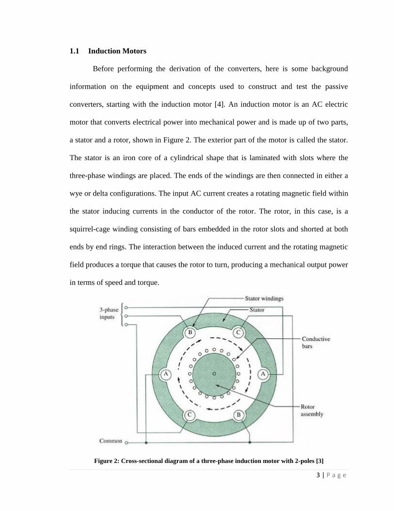
1.1 Induction Motors

Before performing the derivation of the converters, here is some background

information on the equipment and concepts used to construct and test the passive

converters, starting with the induction motor [4]. An induction motor is an AC electric

motor that converts electrical power into mechanical power and is made up of two parts,

a stator and a rotor, shown in Figure 2. The exterior part of the motor is called the stator.

The stator is an iron core of a cylindrical shape that is laminated with slots where the

three-phase windings are placed. The ends of the windings are then connected in either a

wye or delta configurations. The input AC current creates a rotating magnetic field within

the stator inducing currents in the conductor of the rotor. The rotor, in this case, is a

squirrel-cage winding consisting of bars embedded in the rotor slots and shorted at both

ends by end rings. The interaction between the induced current and the rotating magnetic

field produces a torque that causes the rotor to turn, producing a mechanical output power

in terms of speed and torque.

Figure 2: Cross-sectional diagram of a three-phase induction motor with 2-poles [3]

4 | P a g e

Induction motors come in two different phase modes: single-phase and three-

phase. Single-phase motors use a single alternating current and voltage whereas three-

phase motors use three alternating currents and voltages that are all out of phase by 120˚.

Within the three-phase motor, there are three separate windings that are electrically

spaced apart by 120˚. This induces a torque in the rotor that causes the rotor to constantly

“chase” the stator magnetic field to try and align with it. With three-phase power, the

supply is never able to drop to zero. This makes it possible to provide a more constant

power, whereas the single phase the power is at zero three different times during one

cycle [5]. Due to the more constant of power, three-phase power makes it easier to start

the motor and provide a better starting torque.

Figure 3: Block diagram of three-phase induction motor

The top level diagram of a three-phase system is shown in Figure 3. The three-

phase input consists of three voltages, Van, Vbn and Vcn, all with the same amplitude value

but each out of phase by 120˚. Looking at the system at a lower level, there are two

possible winding configurations. The most common is the wye configuration, shown in

5 | P a g e

Figure 4. There are three lines connected from the source to the motor, and a neutral point

where the windings are connected to each other. The three-phase input voltages are

applied to the three windings and cause a flow of current. The summation of the three

phase currents should equal zero if they are equal in magnitude and perfectly separated

by 120˚. If there is any imbalance, the summation of the current will not equal zero and

the neutral provides a return path to the source for the extra current. As the torque of the

motor changes within the motor, the impedance and the current of each winding changes.

Figure 4: Block diagram of wye-connected three-phase induction motor windings

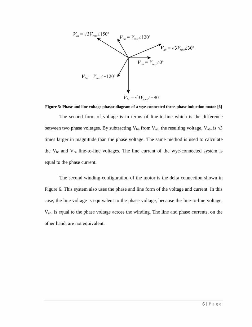
There are two forms of three-phase voltage and current for a wye-connected

motor. The first form is phase voltage, having a magnitude of the voltage across the

winding impedance, which is the source voltage in reference to the neutral point of the

motor. The reference voltage has a phase of 0˚, and the other two voltages are out of

phase by ±120˚. This relationship can be seen in Figure 5, plotting the voltage vectors on

an imaginary versus phase plot.

6 | P a g e

Figure 5: Phase and line voltage phasor diagram of a wye-connected three-phase induction motor [6]

The second form of voltage is in terms of line-to-line which is the difference

between two phase voltages. By subtracting Vbn from Van, the resulting voltage, Vab, is √3

times larger in magnitude than the phase voltage. The same method is used to calculate

the Vbc and Vca line-to-line voltages. The line current of the wye-connected system is

equal to the phase current.

The second winding configuration of the motor is the delta connection shown in

Figure 6. This system also uses the phase and line form of the voltage and current. In this

case, the line voltage is equivalent to the phase voltage, because the line-to-line voltage,

Vab, is equal to the phase voltage across the winding. The line and phase currents, on the

other hand, are not equivalent.

7 | P a g e

Figure 6: Block diagram of delta-connected three-phase induction motor windings

The line current entering into the motor has the magnitude of the source current,

out of phase by 120˚. When it enters the motor, it splits into the two directions creating

the phase current, flowing through the windings. The magnitude of the phase current is

√3 times smaller and leads the line current by 30˚, shown in Figure 7.

Figure 7: Phase and line voltage phasor diagram of delta-connected three-phase induction motor [6]

8 | P a g e

The entire system of an induction motor can be characterized by its input voltage

(Vin), input current (Iin), real input power (Pin), reactive input power (Qin), power factor

(pf), speed (n), and torque (T). The reactive power is due to the imaginary impedance

element in the load, which is this case is the inductance of the winding. The real power is

due to the real component of the load, which is the resistance of the motor winding.

Figure 8 displays the characteristics of the real and reactive input power for an

induction motor in reference of the torque that is introduced to the system. This is the

experimental data for a 1/3hp, three-phase induction motor with full load properties of

208VLL, 1725rpm and 1.4A. The relationship in Figure 8 shows that as the torque

increases from no load, the reactive power stays relatively constant whereas the real

power increases linearly. The dip is due to experimental error and should be in line with

the linear relationship.

Figure 8: Real (P) and reactive (Q) power versus torque of a 1/3HP three-phase induction motor

0

50

100

150

200

250

300

350

400

450

500

0.00 5.00 10.00 15.00 20.00

Po

wer

(W

or

VA

R)

Torque (inlbs)

Real and Reactive Power vs Torque

P

Q

9 | P a g e

1.1.1 Winding Models

The equivalent circuit model for an induction motor, shown in Figure 9, follows

the IEEE Standard 112 [7]. The stator resistance and reactance correspond with R1 and

X1, and the rotor resistance and reactance correspond with R2 and X2. The mutual

inductance of the stator and the rotor is depicted as Xm. The core resistance, Rc, can

typically be neglected when it is much larger than the mutual inductance, causing the

parallel combination equal the mutual reactance.

Figure 9: IEEE standard equivalent circuit of a three-phase induction motor winding

The “s” in the denominator of the rotor resistance corresponds to relative motion

between the rotor and the stator called the slip. To understand the affect of the slip on the

equivalent circuit it is important to know how the torque changes with the loading of the

motor. At first the motor is operating at no load, running close to the speed of the

magnetic field called the synchronous speed. The net magnetic field in the machine is

produced by the magnetization current flowing through the motors equivalent circuit. The

magnetization current and field is proportional to the induced voltage on the rotor side of

the air gap between the stator and the rotor. If the induced voltage is held constant then

the magnetic field is held constant. As the load varies on the motor, the induced voltage

changes because of the stator impedances cause varying voltage drops with the load.

10 | P a g e

Since the voltage drops are relatively small, the rotor induced voltage remains almost

constant with varying loads.

At no load, the rotor slip is very small so the relative motion of the rotor and the

magnetic fields, and rotor frequency is also small. Due to the slow relative motion, the

induced voltage in the rotor’s cage and resulting current is very small. Since the rotor’s

reactance is also small, the maximum rotor current is almost in phase with the rotor’s

induced voltage, producing a very small rotor magnetic field with a phase slightly greater

than the 90˚ behind the total magnetic field of the system. This means that the magnetic

field on the stator side must be very large to be able to supply the full magnetic field.

Since the current is directly related to the magnetic field, the stator current is very large at

no load. The induced torque of the rotor is the cross product between the total and rotor’s

magnetic field, resulting in a very small torque due to the small magnetic field in the

rotor but it is large enough to overcome the rotational losses and turn the rotor.

As the load on the motor increases the motor speed falls. Since the motor speed

decreases, there is more relative motion between the rotor and the stator, increasing the

slip. The greater relative motion also produces a stronger rotor voltage and in turn

increases the rotor current. With a larger rotor current, the magnetic field of the rotor

increases, increasing the induced torque of the rotor. This is why it is suggested that the

slip of the motor to stay under 5%, otherwise the increase in current will be too high

causing power loss and heating of the windings possibly damaging the system.

To obtain the equivalent circuit components three tests must be performed: No

Load, DC and Locked Rotor. The no load test measures the rotational losses of the motor

11 | P a g e

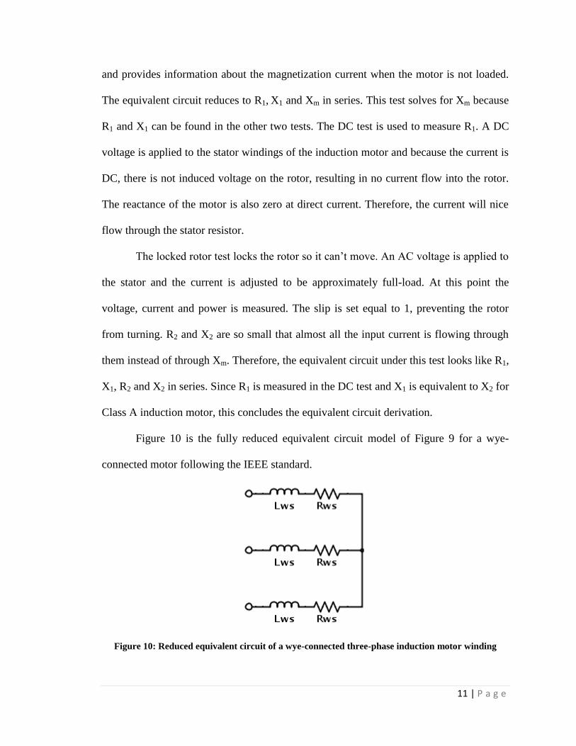
and provides information about the magnetization current when the motor is not loaded.

The equivalent circuit reduces to R1, X1 and Xm in series. This test solves for Xm because

R1 and X1 can be found in the other two tests. The DC test is used to measure R1. A DC

voltage is applied to the stator windings of the induction motor and because the current is

DC, there is not induced voltage on the rotor, resulting in no current flow into the rotor.

The reactance of the motor is also zero at direct current. Therefore, the current will nice

flow through the stator resistor.

The locked rotor test locks the rotor so it can’t move. An AC voltage is applied to

the stator and the current is adjusted to be approximately full-load. At this point the

voltage, current and power is measured. The slip is set equal to 1, preventing the rotor

from turning. R2 and X2 are so small that almost all the input current is flowing through

them instead of through Xm. Therefore, the equivalent circuit under this test looks like R1,

X1, R2 and X2 in series. Since R1 is measured in the DC test and X1 is equivalent to X2 for

Class A induction motor, this concludes the equivalent circuit derivation.

Figure 10 is the fully reduced equivalent circuit model of Figure 9 for a wye-

connected motor following the IEEE standard.

Figure 10: Reduced equivalent circuit of a wye-connected three-phase induction motor winding

12 | P a g e

Another method to calculate the fully reduced equivalent circuit is from the

measured real and reactive input power of the motor. Each motor winding has equivalent

properties leading to even distribution of real and reactive powers through each winding

from the total input power. To obtain the real and reactive input power for each winding,

divide each total input power by three.

By using the input phase voltage or line current, the reactance (XLWS) and

resistance (RWS) of each winding can be calculated by using the equations below.

1.1.2 Series-to-Parallel Winding Component Transformation

As discussed previously, the current through each winding changes as the torque

is increased. Therefore, when solving for the impedances for the series winding

components, both the inductance and resistance values change with the varying current.

13 | P a g e

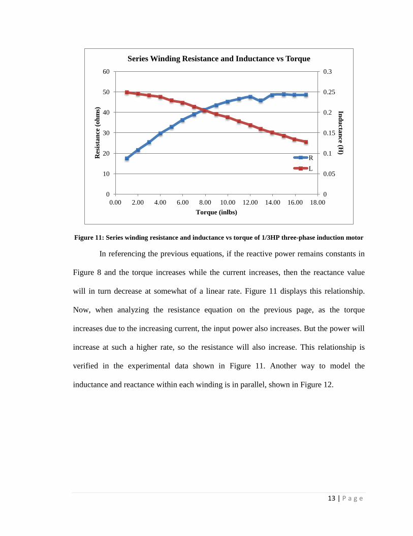
Figure 11: Series winding resistance and inductance vs torque of 1/3HP three-phase induction motor

In referencing the previous equations, if the reactive power remains constants in

Figure 8 and the torque increases while the current increases, then the reactance value

will in turn decrease at somewhat of a linear rate. Figure 11 displays this relationship.

Now, when analyzing the resistance equation on the previous page, as the torque

increases due to the increasing current, the input power also increases. But the power will

increase at such a higher rate, so the resistance will also increase. This relationship is

verified in the experimental data shown in Figure 11. Another way to model the

inductance and reactance within each winding is in parallel, shown in Figure 12.

0

0.05

0.1

0.15

0.2

0.25

0.3

0

10

20

30

40

50

60

0.00 2.00 4.00 6.00 8.00 10.00 12.00 14.00 16.00 18.00

Ind

ucta

nce (H

)

Res

ista

nce

(o

hm

s)

Torque (inlbs)

Series Winding Resistance and Inductance vs Torque

R

L

14 | P a g e

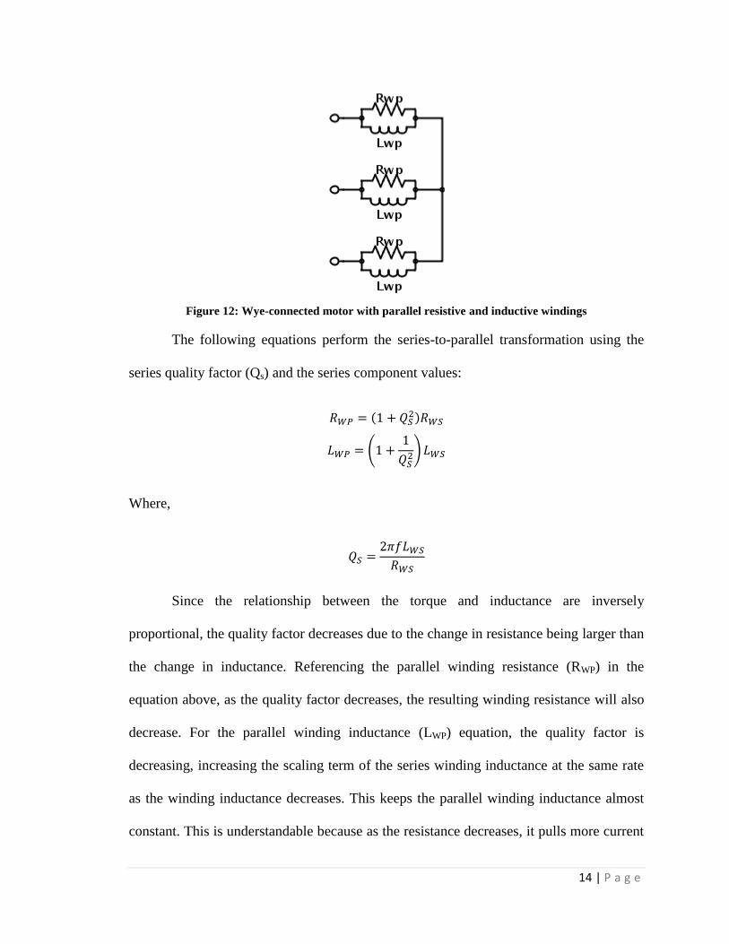
Figure 12: Wye-connected motor with parallel resistive and inductive windings

The following equations perform the series-to-parallel transformation using the

series quality factor (Qs) and the series component values:

Where,

Since the relationship between the torque and inductance are inversely

proportional, the quality factor decreases due to the change in resistance being larger than

the change in inductance. Referencing the parallel winding resistance (RWP) in the

equation above, as the quality factor decreases, the resulting winding resistance will also

decrease. For the parallel winding inductance (LWP) equation, the quality factor is

decreasing, increasing the scaling term of the series winding inductance at the same rate

as the winding inductance decreases. This keeps the parallel winding inductance almost

constant. This is understandable because as the resistance decreases, it pulls more current

15 | P a g e

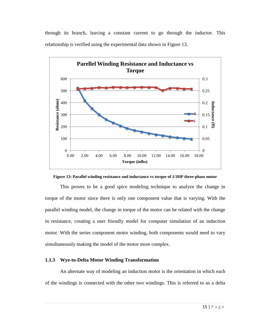
through its branch, leaving a constant current to go through the inductor. This

relationship is verified using the experimental data shown in Figure 13.

Figure 13: Parallel winding resistance and inductance vs torque of 1/3HP three-phase motor

This proves to be a good spice modeling technique to analyze the change in

torque of the motor since there is only one component value that is varying. With the

parallel winding model, the change in torque of the motor can be related with the change

in resistance, creating a user friendly model for computer simulation of an induction

motor. With the series component motor winding, both components would need to vary

simultaneously making the model of the motor more complex.

1.1.3 Wye-to-Delta Motor Winding Transformation

An alternate way of modeling an induction motor is the orientation in which each

of the windings is connected with the other two windings. This is referred to as a delta

0

0.05

0.1

0.15

0.2

0.25

0.3

0

100

200

300

400

500

600

0.00 2.00 4.00 6.00 8.00 10.00 12.00 14.00 16.00 18.00

Ind

ucta

nce (H

)

Res

ista

nce

(o

hm

s)

Torque (inlbs)

Parellel Winding Resistance and Inductance vs

Torque

R

L

16 | P a g e

configuration. Below are the equations used to transform a wye-connected motor into a

delta-connected motor.

Figure 14: Wye-to-delta transformation of parallel resistive and inductive induction motor windings

By using the delta configuration, it is easier to power factor correct the motor. In

power factor correction, capacitors are added in parallel to each winding. Since capacitors

are opposite in polarity with inductors it reduces the inductance of the winding down to

zero and in turn reduces the reactive power down to zero. This is valuable because it will

require less power from the source, only transferring real power to the load.

1.2 Passive Single to Three-Phase Conversion Topologies

There are three passive single to three-phase conversion topologies that will be

analyzed in this study. They are referenced as the Cal Poly (CP) converter,

Marinus/Malengret converter and the Smith converter. The first two were discovered for

17 | P a g e

a previous study to design a high efficiency portable air conditioner, which was

sponsored by Lawrence Berkeley National Labs and the Department of Energy [8]. The

third conversion network, proposed by an inventor Otto Smith, shows similarities in

voltage characteristics and motor connections to the Marinus/Malengret converter. Due

to these similarities, this thesis will attempt to prove the equivalency of the two motors.

1.2.1 Cal Poly Converter

The first single to three-phase conversion network is called the Cal Poly converter

and is named after California Polytechnic State University in San Luis Obipso, where the

design was developed [8]. The network consists of four conversion components for a

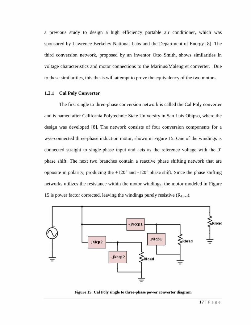
wye-connected three-phase induction motor, shown in Figure 15. One of the windings is

connected straight to single-phase input and acts as the reference voltage with the 0˚

phase shift. The next two branches contain a reactive phase shifting network that are

opposite in polarity, producing the +120˚ and -120˚ phase shift. Since the phase shifting

networks utilizes the resistance within the motor windings, the motor modeled in Figure

15 is power factor corrected, leaving the windings purely resistive (RLoad).

Figure 15: Cal Poly single to three-phase power converter diagram

18 | P a g e

When LC networks are present on their own, they introduce a phase shift of 180˚

as demonstrated by the below transfer function. The LC network behaves as a voltage

divider and inverter if the magnitude of the capacitor’s reactance is larger than the

inductor’s.

Figure 16: Phase conversion results of LC network

Each branch of the conversion network is derived individually and utilizes its

transfer function to derive the components. Figure 17 displays the top branch, which

introduces the +120˚ phase shift.

Figure 17: +120˚ phase shifting branch of Cal Poly converter

19 | P a g e

The transfer function of the Figure 17 consists of the output voltage over the input

voltage of the branch. Since the current going through the capacitor is the same as the

current going through the parallel combination of the inductor and resistor, we can reduce

the transfer function in terms of the output impedance over the total impedance of the

circuit.

By reducing the equation further, a “j” component is left in the numerator and a

complex relationship in the denominator. The “j” component in the numerator introduces

a +90˚ phase shift, therefore to achieve the full +120˚ phase shift the denominator needs

to experience a -30˚ phase shift. By setting the denominator equal to the complex

rectangular form of -30˚ and matching the real and imaginary coefficients from both sides

of the equation, we can derive the value of each conversion component in terms of the

resistance within the motor winding.

The same method is performed on Figure 18, the bottom branch of the conversion

network which introduces the -120˚.

20 | P a g e

Figure 18: -120˚ phase shifting branch of Cal Poly Converter

In this case, the reduced equation contains a “-j” component in the numerator,

introducing a -90˚ phase shift. To achieve the full -120˚ phase shift for the branch, it is

necessary for the complex relationship in the denominator to have a +30˚ phase shift. By

setting the denominator equal to the complex rectangular form of +30˚ and matching the

real and imaginary coefficients from both sides of the equation, each conversion

component can be derived in terms of the resistance within the motor winding.

1.2.2 Marinus/Malengret Converter

The second single to three-phase conversion network is called the

Marinus/Malengret (MM) converter. It is referenced after the authors of an IEEE article

in which Stuart Marinus and Michel Malangret proposed the design [11]. The network

21 | P a g e

uses a delta connected induction motor with two conversion components, one capacitor

and one inductor. Referencing the network displayed Figure 19, both of the conversion

components are placed across the main winding and supply, with each individual

component connected in parallel with the other two windings. The motor is power factor

corrected, leaving the windings purely resistive. The conversion network is displayed on

the left hand side of Figure 19 and the power factor corrected motor is on the right hand

side.

Figure 19: Block diagram of Marinus/Malengret converter and power factor corrected motor

The approach to derive the Marinus/Malengret converter components involves

combining the inductor and capacitor with their parallel winding resistance and using the

current relationship through that line. The combined impedance is displayed below in

Figure 20.

22 | P a g e

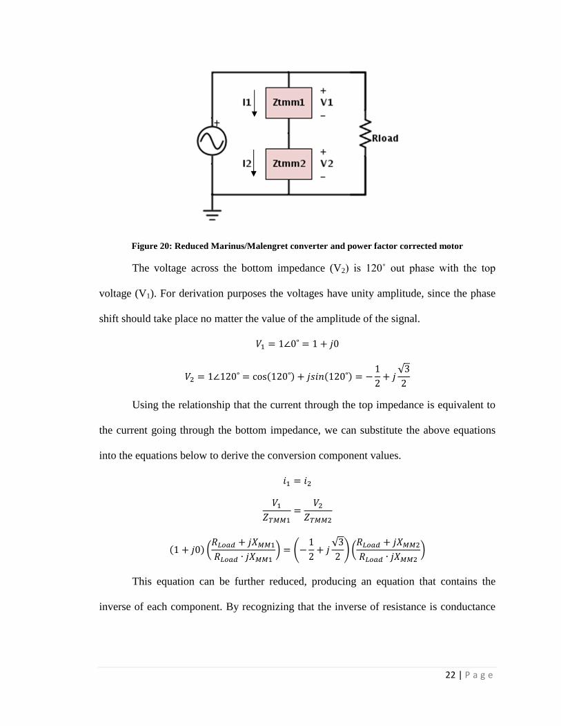
Figure 20: Reduced Marinus/Malengret converter and power factor corrected motor

The voltage across the bottom impedance (V2) is 120˚ out phase with the top

voltage (V1). For derivation purposes the voltages have unity amplitude, since the phase

shift should take place no matter the value of the amplitude of the signal.

Using the relationship that the current through the top impedance is equivalent to

the current going through the bottom impedance, we can substitute the above equations

into the equations below to derive the conversion component values.

This equation can be further reduced, producing an equation that contains the

inverse of each component. By recognizing that the inverse of resistance is conductance

23 | P a g e

(G) and the inverse of reactance is susceptance (B), we can make those substitutions and

more easily derive the conversion components.

By matching the real and imaginary parts of each side, the two following equations are

produced:

By adding the two equations together, we get the equation below, which can be

fully reduced into terms of the conductance.

The same can be done by subtracting the equations. This time it is reduced down

to a relationship between the susceptances, and then a relationship between the

conversion component reactances. The resulting relationship shows that the two

reactances are opposite in polarity verifying the use of a capacitor and an inductor in the

conversion network.

24 | P a g e

By converting the suspectance and conductance back into reactance and resistance

and making the substitutions into the above equation, the final derivation of the

conversion component values is possible. The values are shown in the equations below.

1.3 Otto Smith Converter

The third conversion circuit is called the Smith converter. This converter is named

after its inventor Otto Smith and he received a patent for this design in 1994 [12]. Smith

has done extensive research related to solar generators, wind generators and high

efficiency motors. He has received 15 patents for devices that generate or conserve

energy. The Smith converter was designed for a standard three-phase induction motor.

Two of the motor windings are connected across a single phase power supply, and a

center-tapped autotransformer is connected between the second and third motor winding.

A diagram of the Smith conversion network with a three-phase motor is shown in Figure

21.

25 | P a g e

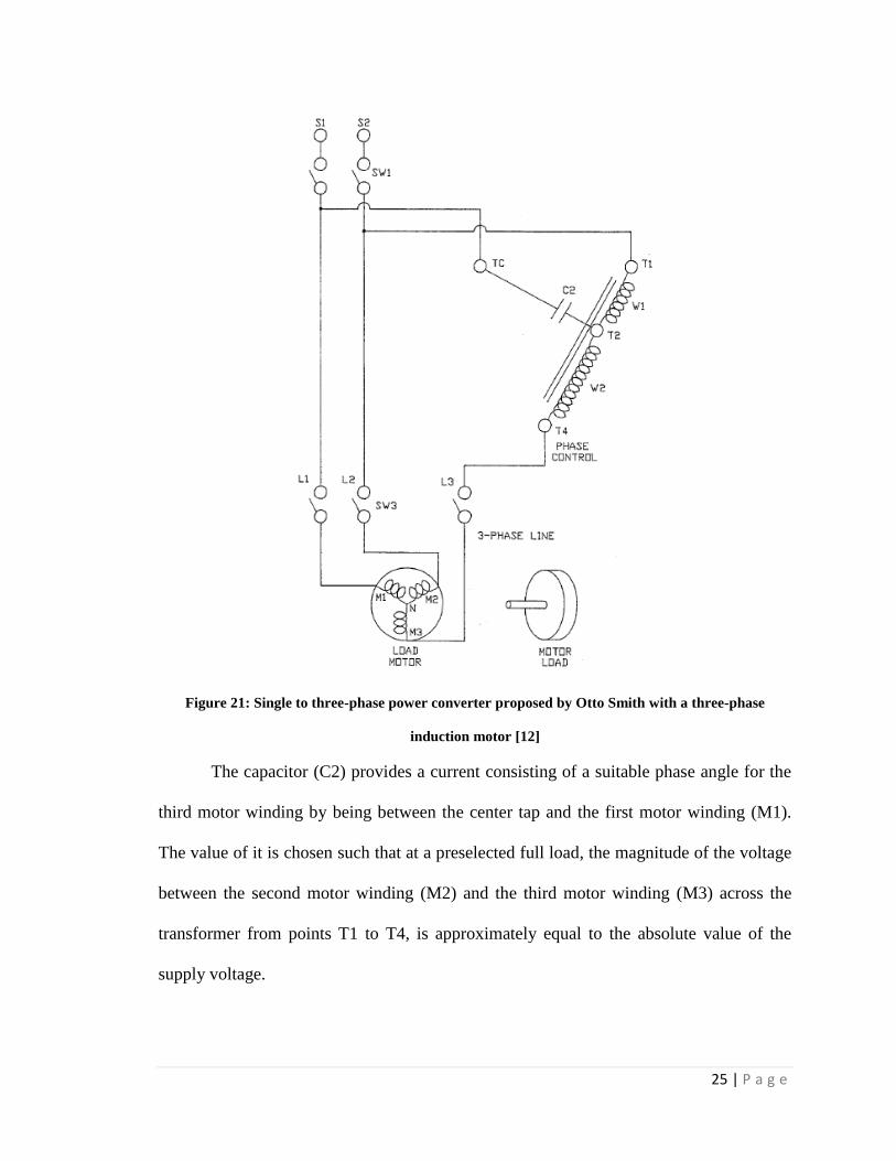
Figure 21: Single to three-phase power converter proposed by Otto Smith with a three-phase

induction motor [12]

The capacitor (C2) provides a current consisting of a suitable phase angle for the

third motor winding by being between the center tap and the first motor winding (M1).

The value of it is chosen such that at a preselected full load, the magnitude of the voltage

between the second motor winding (M2) and the third motor winding (M3) across the

transformer from points T1 to T4, is approximately equal to the absolute value of the

supply voltage.

26 | P a g e

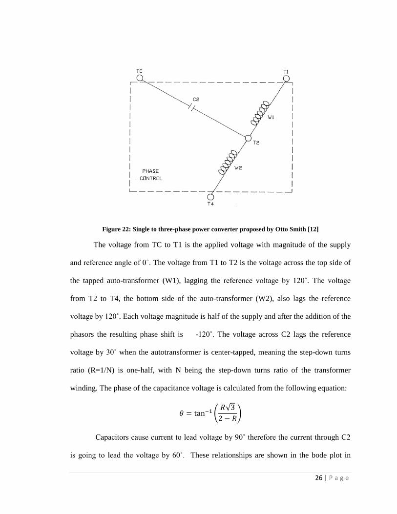
Figure 22: Single to three-phase power converter proposed by Otto Smith [12]

The voltage from TC to T1 is the applied voltage with magnitude of the supply

and reference angle of 0˚. The voltage from T1 to T2 is the voltage across the top side of

the tapped auto-transformer (W1), lagging the reference voltage by 120˚. The voltage

from T2 to T4, the bottom side of the auto-transformer (W2), also lags the reference

voltage by 120˚. Each voltage magnitude is half of the supply and after the addition of the

phasors the resulting phase shift is -120˚. The voltage across C2 lags the reference

voltage by 30˚ when the autotransformer is center-tapped, meaning the step-down turns

ratio (R=1/N) is one-half, with N being the step-down turns ratio of the transformer

winding. The phase of the capacitance voltage is calculated from the following equation:

Capacitors cause current to lead voltage by 90˚ therefore the current through C2

is going to lead the voltage by 60˚. These relationships are shown in the bode plot in

27 | P a g e

Figure 23. By closing the triangle in the bode plot, the resulting phasor of T4 to TC is

leading the input by 120˚, providing the third phase of +120˚.

Figure 23: Current and Voltage phasor diagram of Otto Smith’s conversion network [12]

This conversion can also be performed using a two winding or multiple winding

transformer in place of the center-tapped autotransformer, shown in Figure 24. The

winding between T2 and T1 has the same voltage as W1 and the same current from C2,

as in the auto-transformer design. The voltage of the secondary winding, from T1 to T4,

has the same magnitude as the input voltage with a lagging phase angle of 120˚, same as

W2 from the previous design. The step-down ratio still equals the inverse of the step-

down ratio of the transformer winding, thus the two winding transformer has an effective

center-tap or, in more general terms, an intermediate tap as in an autotransformer.

28 | P a g e

Figure 24: Alternate conversion network proposed by Otto Smith utilizing a two winding

transformer [12]

1.4 Derivation of Marinus/Malengret Converter from Induction Motor

To begin the derivation of the values of the Marinus/Malengret converter

components, the motor characteristics at the operating load is needed.

Table 1 is the data from a motor loading test from no load to full load. The rotor’s

speed (nr), input line-to-line RMS voltage (VL-L), RMS line current (IL), input real power

(Pin) and input reactive power (Qin) were collected as the torque (T) increased from 1 in-

lbs to 17 in-lbs for a 1/3 HP three-phase induction motor. The 12in-lbs operating torque is

calculated by using the equation below.

29 | P a g e

Table 1: Measurement results of 1/3HP three-phase induction motor

T [inlbs] nr [RPM] VL-L [V] IL [A] Pin[W] Qin [VAR]

0.00 1797 210.6 1.290 77.8 471

1.02 1795 210.7 1.290 87.1 469

2.01 1791 210.7 1.291 108.2 463

3.00 1788 210.6 1.300 129.0 462

4.00 1784 210.6 1.308 152.1 460

5.00 1781 210.7 1.330 174.4 459

5.98 1777 210.6 1.345 196.6 457

7.01 1772 210.4 1.371 220.3 455

7.92 1769 210.6 1.398 242.0 453

8.99 1764 210.3 1.430 267.0 453

9.99 1760 210.4 1.464 291.0 456

11.00 1755 210.3 1.501 315.0 454

12.01 1751 210.2 1.543 340.0 455

12.94 1747 210.1 1.587 346.0 454

13.95 1741 210.0 1.636 389.0 456

14.99 1736 210.0 1.684 415.0 458

15.93 1732 210.1 1.736 439.0 458

16.97 1726 210.0 1.789 467.0 462

Figure 25 is the layout of the non-reduced Marinus/Malengret converter. On the

right side of the figure is the delta-connected three-phase motor utilizing the parallel

model for the non-power factor corrected windings. To the left of the motor are the power

factor (PF) correction capacitors. Due to the choice in motor winding connection, the

value of these components can be read directly from the schematic. Since the PF

components are in parallel with the winding inductances, reactance of the PF components

are equivalent to the negative reactance of the winding inductance (LDP). This will

eliminate the effects of the inductance, leaving the windings completely resistive and

eliminate the reactive power. On the left side of Figure 25, is the single to three-phase

conversion network and its components were derived in Section 1.2.2.

30 | P a g e

Figure 25: Marinus/Malengret converter with delta-connected motor and power factor correction

network

Below are the equations for the previously derived reactances of conversion

network and PF components, in terms of the motor resistance and reactance at the point

of operation.

Now that the values have been derived, the circuit can be simplified to reduce the

number of components being used. Due to the parallel connection of the inductor of the

conversion network and a PF capacitor, an equivalent converter inductance is derived.

31 | P a g e

Due to the parallel connection of the capacitor of the conversion network and

another PF capacitor, an equivalent converter capacitance is derived.

To verify that the calculations are correct, LTspice simulations were performed

using a sinusoidal voltage input with and amplitude of 170pk at 60Hz. Figure 26 displays

the schematic with the calculated numerical values. From left to right is single-phase

source, the delta-connected motor and the converter.

Figure 26: LTspice model of reduced MM converter with 1/3HP delta-connected motor

32 | P a g e

Figure 27: Single-phase source voltage with MM converter and 1/3HP delta-connected motor

Figure 28: Three-phase voltage delivered from MM converter to 1/3HP delta-connected motor

Figure 29: Single-phase source current with MM converter and 1/3HP delta-connected motor

Figure 30: Three-phase current delivered from MM converter to 1/3HP delta-connected motor

33 | P a g e

Figure 27 displays the voltage from the single-phase source driving the

Marinus/Malengret converter and the 1/3HP delta-connected motor. This waveform is

also the reference voltage in Figure 28 with peak amplitude of 170V. Figure 28 displays

the three-phase voltage delivered from the converter to the motor in Figure 26. The green

waveform is the reference voltage with a phase of 0˚, the blue waveform is the voltage

between the top and middle line of the system shifted by +120˚, and the red waveform is

the voltage between the middle and bottom line shifted by -120˚, all with the amplitude of

170V.

Figure 29 displays the current from the single-phase source driving the

Marinus/Malengret converter and the 1/3HP delta-connected motor. Its amplitude is

1.28A with an offset of 0.89A, increasing the peak current to 2.17A. This offset is due to

the simulation parameters set by LTspice. Without the current initialized to zero, this

circuit experiences a DC offset in the source current. Therefore, by placing a voltage

controlled variable resistor, called a varistor, between the single-phase source and the

remaining components in the system, the voltage will gradually increase from zero,

initializing both the voltage and current to zero.

Figure 31: Model of reduced MM converter with 1/3HP delta-connected motor with varistor

34 | P a g e

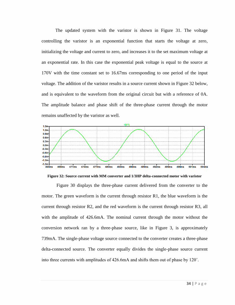
The updated system with the varistor is shown in Figure 31. The voltage

controlling the varistor is an exponential function that starts the voltage at zero,

initializing the voltage and current to zero, and increases it to the set maximum voltage at

an exponential rate. In this case the exponential peak voltage is equal to the source at

170V with the time constant set to 16.67ms corresponding to one period of the input

voltage. The addition of the varistor results in a source current shown in Figure 32 below,

and is equivalent to the waveform from the original circuit but with a reference of 0A.

The amplitude balance and phase shift of the three-phase current through the motor

remains unaffected by the varistor as well.

Figure 32: Source current with MM converter and 1/3HP delta-connected motor with varistor

Figure 30 displays the three-phase current delivered from the converter to the

motor. The green waveform is the current through resistor R1, the blue waveform is the

current through resistor R2, and the red waveform is the current through resistor R3, all

with the amplitude of 426.6mA. The nominal current through the motor without the

conversion network ran by a three-phase source, like in Figure 3, is approximately

739mA. The single-phase voltage source connected to the converter creates a three-phase

delta-connected source. The converter equally divides the single-phase source current

into three currents with amplitudes of 426.6mA and shifts them out of phase by 120˚.

35 | P a g e

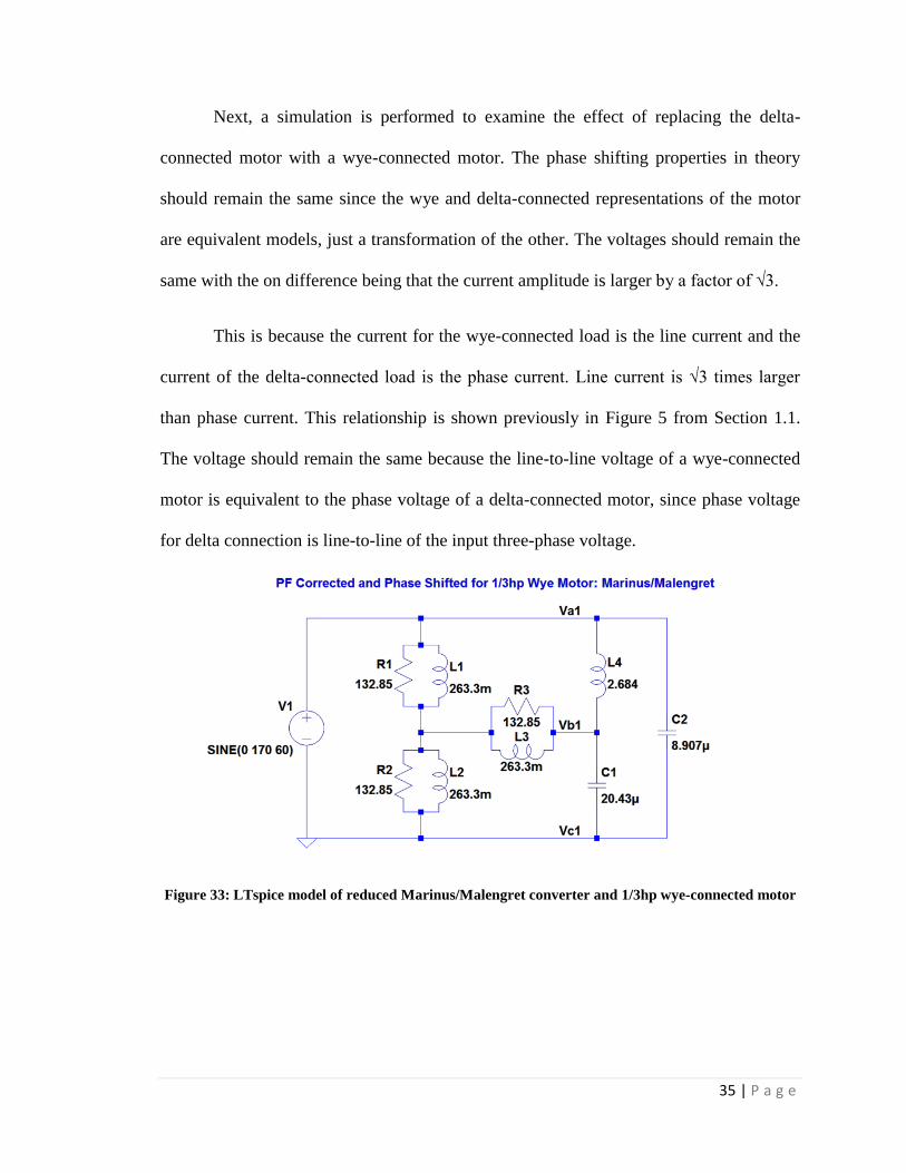
Next, a simulation is performed to examine the effect of replacing the delta-

connected motor with a wye-connected motor. The phase shifting properties in theory

should remain the same since the wye and delta-connected representations of the motor

are equivalent models, just a transformation of the other. The voltages should remain the

same with the on difference being that the current amplitude is larger by a factor of √3.

This is because the current for the wye-connected load is the line current and the

current of the delta-connected load is the phase current. Line current is √3 times larger

than phase current. This relationship is shown previously in Figure 5 from Section 1.1.

The voltage should remain the same because the line-to-line voltage of a wye-connected

motor is equivalent to the phase voltage of a delta-connected motor, since phase voltage

for delta connection is line-to-line of the input three-phase voltage.

Figure 33: LTspice model of reduced Marinus/Malengret converter and 1/3hp wye-connected motor

36 | P a g e

Figure 34: Single-phase source voltage with MM converter and 1/3HP wye-connected motor

Figure 35: Three-phase voltage delivered from MM converter to 1/3HP wye-connected motor

Figure 36: Single-phase source current with MM converter and 1/3HP wye-connected motor

Figure 37: Three-phase current delivered from MM converter to 1/3HP wye-connected motor

37 | P a g e

Figure 34 displays the voltage from the single-phase source driving the

Marinus/Malengret converter and the 1/3HP wye-connected motor. This waveform is

also the reference voltage in Figure 35 with peak amplitude of 170V. Figure 35 displays

the three-phase voltage delivered from the converter to the motor in Figure 33. The green

waveform is the reference voltage with a phase of 0˚, the blue waveform is the voltage

between the top and middle line of the system shifted by +120˚, and the red waveform is

the voltage between the middle and bottom line shifted by -120˚, all with the amplitude of

170V.

Figure 36 displays the current from the single-phase source driving the

Marinus/Malengret converter and the 1/3HP wye-connected motor. Its amplitude is

1.28A with an offset of 0.89A, increasing the peak current to 2.17A. This is due to the

same reason as the system with delta-connected motor. The current is not initialized to

zero by the simulation settings. Therefore, we will incorporate the varistor into the

network to initialize the voltage and the current. This is shown in Figure 38, below.

Figure 38: LTspice model of reduced MM converter and 1/3hp wye-connected motor with varistor

38 | P a g e

The exponential peak voltage controlling the varistor is equal to the source at

170V and the time constant it set to 16.67ms corresponding to one period of the input

voltage. The addition of the varistor produces the source current waveform shown in

Figure 39 below, and is equivalent to the waveform from the original circuit, but with the

reference set at 0A. The amplitude balance and phase shift of the three-phase current in

the motor remains unaffected by the varistor.

Figure 39: Source current with MM converter and 1/3HP wye-connected motor with varistor

The theory of the current holds true and is shown in Figure 37, displaying the

current simulation of the motor of Figure 33. The green waveform is the current through

resistor R1, the blue waveform is the current through resistor R2, and the red waveform is

the current through resistor R3, all with the amplitude of 738.6mA. These peak currents

equate to about √3 times the peak currents of the delta connected motor, which is correct

since a delta to wye transformation is being performed. The single-phase voltage source

connected to the converter creates a three-phase delta-connected source. The converter

equally divides the single-phase source current into three currents with amplitudes of

426.6mA, equivalent to 738.6mA line current for the motor, and shifts them out of phase

by 120˚. The waveforms extracted from the wye and delta-connected motors exhibit the

same phase shift and balance in waveform amplitudes. From that we can conclude that

the conversion network can be used for both motor configurations.

39 | P a g e

Chapter 2: Marinus/Malengret to Smith Transformation

From a top level block diagram perspective, the three conversion networks can be

separated into two categories. The converter either has three or four connection lines

between itself and the motor. The two converters that fall under the three connection line

category are the Marinus/Malengret converter and the Smith converter. Another detail to

notice from Figure 40 is that the output of the converters would need to be equivalent to

properly supply the required power to the motor. To achieve the same output, there

should be a correlation between the two converters. This next step is to prove the

equivalency of the two converters that were proposed by Stuart Marinus and Michel

Malengret, and Otto Smith.

Figure 40: Marinus/Malengret and Smith conversion network comparison

The Marinus/Malengret converter utilizes a delta network for its components and

the Smith converter utilizes a wye network. The wye configuration of the Smith converter

might not be immediately apparent, but the tapped auto-transformer can be thought of as

two coupled inductors creating a two winding transformer, as discussed earlier in Section

40 | P a g e

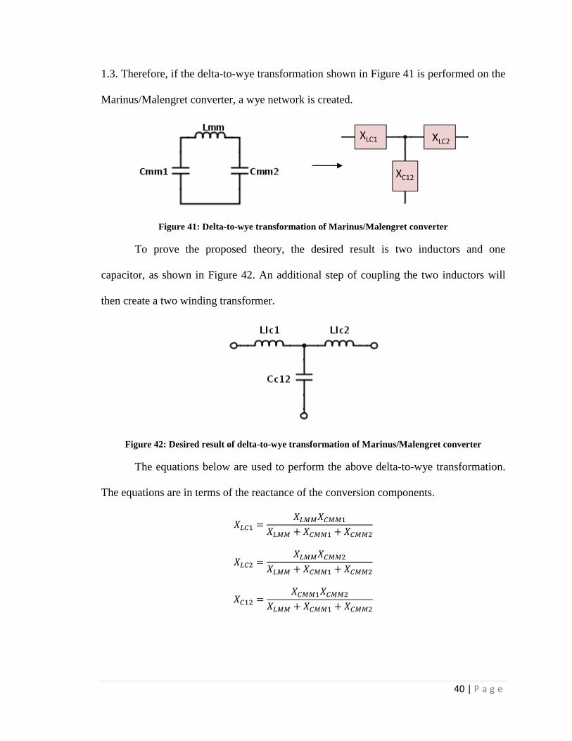
1.3. Therefore, if the delta-to-wye transformation shown in Figure 41 is performed on the

Marinus/Malengret converter, a wye network is created.

Figure 41: Delta-to-wye transformation of Marinus/Malengret converter

To prove the proposed theory, the desired result is two inductors and one

capacitor, as shown in Figure 42. An additional step of coupling the two inductors will

then create a two winding transformer.

Figure 42: Desired result of delta-to-wye transformation of Marinus/Malengret converter

The equations below are used to perform the above delta-to-wye transformation.

The equations are in terms of the reactance of the conversion components.

41 | P a g e

Table 2 displays the calculated wye-network reactances from the above equations

for the components in Figure 41. Also included are the corresponding torques and power

factors of the 1/3hp three-phase induction motor, used previously to derive the

Marinus/Malengret converter. When the motor is operating at its rated torque of 12 in-

lbs, the resulting component reactances include two negative and one positive value.

Table 2: Component results of uncoupled Smith converter with 1/3hp motor

Smith (uncoupled)

T [inlbs] PF XLC1(Ω) XLC2(Ω) XC12(Ω)

1.02 0.185 -100.656 -133.034 -68.279

2.01 0.230 -103.298 -145.109 -61.486

3.00 0.272 -106.535 -158.057 -55.012

4.00 0.318 -111.626 -175.555 -47.697

5.00 0.361 -115.682 -191.813 -39.551

5.98 0.400 -122.454 -213.698 -31.211

7.01 0.439 -130.105 -239.213 -20.997

7.92 0.473 -138.971 -267.560 -10.383

8.99 0.511 -152.458 -308.100 3.183

9.99 0.546 -168.367 -354.466 17.733

11.00 0.574 -191.874 -422.460 38.711

12.01 0.605 -224.797 -515.748 66.153

12.94 0.598 -226.600 -525.718 72.517

13.95 0.654 -360.372 -892.843 172.099

14.99 0.677 -547.808 -1407.556 311.941

15.93 0.697 -1196.323 -3182.455 789.809

16.97 0.717 4470.214 12296.647 -3356.219

These reactances translate into two capacitors and one inductor, shown in Figure

43, which is the opposite of what is desired. The only row on the table that delivers the

desired two inductors and one capacitor has a torque of 16.97in-lbs and has a power

factor of 0.717. From this data, two theories are formulated. Either the motor needs to

have a higher rated torque or it needs to have a higher rated power factor.

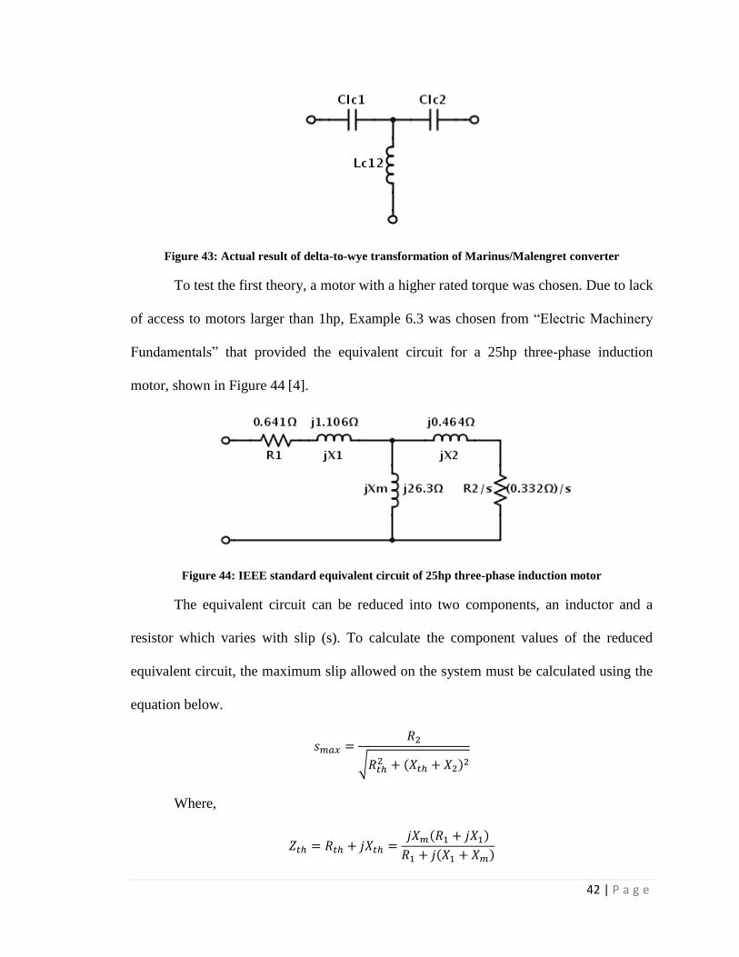
42 | P a g e

Figure 43: Actual result of delta-to-wye transformation of Marinus/Malengret converter

To test the first theory, a motor with a higher rated torque was chosen. Due to lack

of access to motors larger than 1hp, Example 6.3 was chosen from “Electric Machinery

Fundamentals” that provided the equivalent circuit for a 25hp three-phase induction

motor, shown in Figure 44 [4].

Figure 44: IEEE standard equivalent circuit of 25hp three-phase induction motor

The equivalent circuit can be reduced into two components, an inductor and a

resistor which varies with slip (s). To calculate the component values of the reduced

equivalent circuit, the maximum slip allowed on the system must be calculated using the

equation below.

Where,

43 | P a g e

With the range of slip, the winding reactance values are calculated and

transformed into Marinus/Malengret and Smith converter components, recorded in Table

3. The list provides values up to 5% slip because it is highly suggested to stay under that

range. Anything higher will introduce too much current into the system causing a greater

power loss and could possibly damage the motor due to excess heat. The power factor is

also included for each slip value by taking the cosine of the negative phase of the total

impedance of the winding.

Table 3: Component results of Marinus/Malengret and uncoupled Smith converter with 25hp motor

Marinus/Malengret Smith (Uncoupled)

s PF XLmm(Ω) XCmm1(Ω) XCmm2(Ω) XLC1(Ω) XLC2(Ω) XC12(Ω)

0.010 0.610 246.431 -35.276 -82.340 -67.486 -157.521 22.549

0.015 0.742 87.854 -27.581 -80.404 120.368 350.897 -110.161

0.020 0.813 54.517 -22.641 -77.448 27.086 92.650 -38.478

0.022 0.840 46.564 -21.279 -78.377 18.662 68.738 -31.413

0.025 0.854 40.100 -19.212 -73.764 14.570 55.941 -26.801

0.030 0.878 32.084 -16.699 -69.644 9.874 41.182 -21.434

0.035 0.892 27.000 -14.782 -65.336 7.514 33.210 -18.183

0.040 0.901 23.502 -13.277 -61.033 6.141 28.231 -15.949

0.045 0.906 20.958 -12.065 -56.871 5.271 24.843 -14.302

0.050 0.909 19.034 -11.072 -52.935 4.686 22.404 -13.032

The results in the above table provide the desired two inductors and one capacitor

for the Smith converter, starting at a slip of 1.5%. The component values at 2.2% slip are

chosen since that is what was suggested by the example in the textbook. The next step is

to couple the inductors into a two winding transformer. When coupling inductors, a

negative mutual inductance is introduced to the rest of the network and can be drawn as

the connection on the right in Figure 45. By combining the negative mutual inductance

(-Lmutual) and the capacitance (CC12) we get the capacitor in the Smith converter.

44 | P a g e

Figure 45: Uncoupled-to-coupled inductor model of Smith converter

To calculate the coupled inductances, LS1 and LS2, and the mutual inductance, Lm,

the following equations are used, in terms of reactance.

The next step is to solve for the impedance of the first winding of the coupled

inductor, XLS1. The following equation is produced by isolating the mutual inductance in

the top two equations above, setting those resulting equations equal to each other and

then isolating the reactance of the first winding.

The next equation is derived by substituting XLS1 into the original XLS2.

Now we can solve for mutual reactance, XM.

The last step is to solve for the capacitance of the converter. This is done by

adding the negative mutual reactance with the reactance of the capacitor.

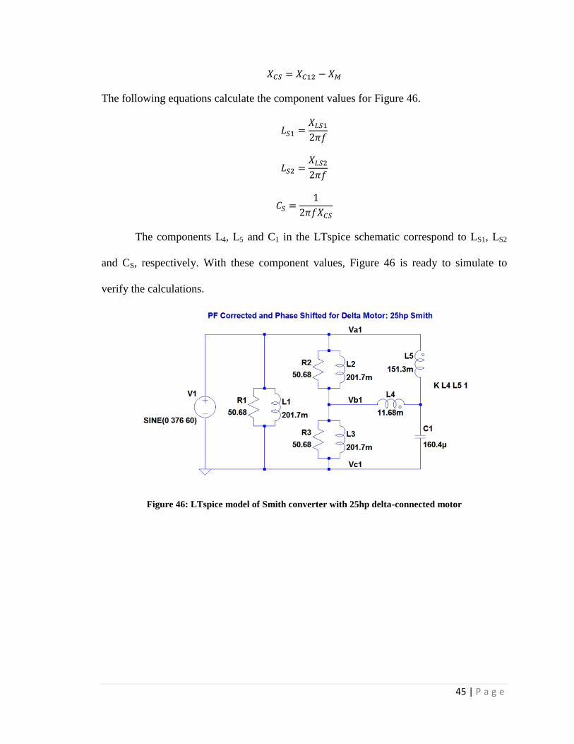
45 | P a g e

The following equations calculate the component values for Figure 46.

The components L4, L5 and C1 in the LTspice schematic correspond to LS1, LS2

and CS, respectively. With these component values, Figure 46 is ready to simulate to

verify the calculations.

Figure 46: LTspice model of Smith converter with 25hp delta-connected motor

46 | P a g e

Figure 47: Single-phase source voltage with Smith converter and 25HP delta-connected motor

Figure 48: Three-phase voltage delivered from Smith converter to 25HP delta-connected motor

Figure 49: Single-phase source current with Smith converter and 25HP delta-connected motor

Figure 50: Three-phase current delivered from Smith converter to 25HP delta-connected motor

47 | P a g e

Figure 47 displays the voltage from the single-phase source driving the Smith

converter and the 25HP delta-connected motor. This waveform is also the reference

voltage in Figure 48 with peak amplitude of 376V. Figure 48 displays the three-phase

voltage delivered from the converter to the motor in Figure 46. The green waveform is

the reference voltage with a phase of 0˚, the blue waveform is the voltage between the top

and middle line of the system shifted by +120˚, and the red waveform is the voltage

between the middle and bottom line shifted by -120˚, all with the amplitude of 376V.

Figure 49 displays the current from the single-phase source driving the Smith

converter and the 25HP delta-connected motor. Its amplitude is 22.26A with an offset of

8.11A, increasing the peak current to 30.37A. This is due to the same reason as the

systems with the Marinus/Malengret converter. The current is not initialized to zero by

the simulation settings. Therefore, we will incorporate a varistor into the network to

initialize the voltage and the current. This is shown in Figure 51, below.

Figure 51: LTspice model of Smith converter with 25hp delta-connected motor with varistor



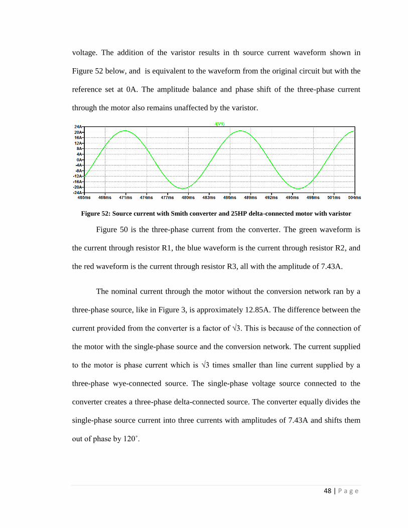
48 | P a g e

voltage. The addition of the varistor results in th source current waveform shown in

Figure 52 below, and is equivalent to the waveform from the original circuit but with the

reference set at 0A. The amplitude balance and phase shift of the three-phase current

through the motor also remains unaffected by the varistor.

Figure 52: Source current with Smith converter and 25HP delta-connected motor with varistor

Figure 50 is the three-phase current from the converter. The green waveform is

the current through resistor R1, the blue waveform is the current through resistor R2, and

the red waveform is the current through resistor R3, all with the amplitude of 7.43A.

The nominal current through the motor without the conversion network ran by a

three-phase source, like in Figure 3, is approximately 12.85A. The difference between the

current provided from the converter is a factor of √3. This is because of the connection of

the motor with the single-phase source and the conversion network. The current supplied

to the motor is phase current which is √3 times smaller than line current supplied by a

three-phase wye-connected source. The single-phase voltage source connected to the

converter creates a three-phase delta-connected source. The converter equally divides the

single-phase source current into three currents with amplitudes of 7.43A and shifts them

out of phase by 120˚.

49 | P a g e

Figure 53: LTspice model of Smith converter with 25hp wye-connected motor


converter and the 25HP wye-connected motor. This waveform is also the reference


voltage delivered from the converter to the motor in Figure 53. The green waveform is

the reference voltage with a phase of 0˚, the blue waveform is the voltage between the top

and middle line of the system shifted by +120˚, and the red waveform is the voltage

between the middle and bottom line shifted by -120˚, all with the amplitude of 376V.

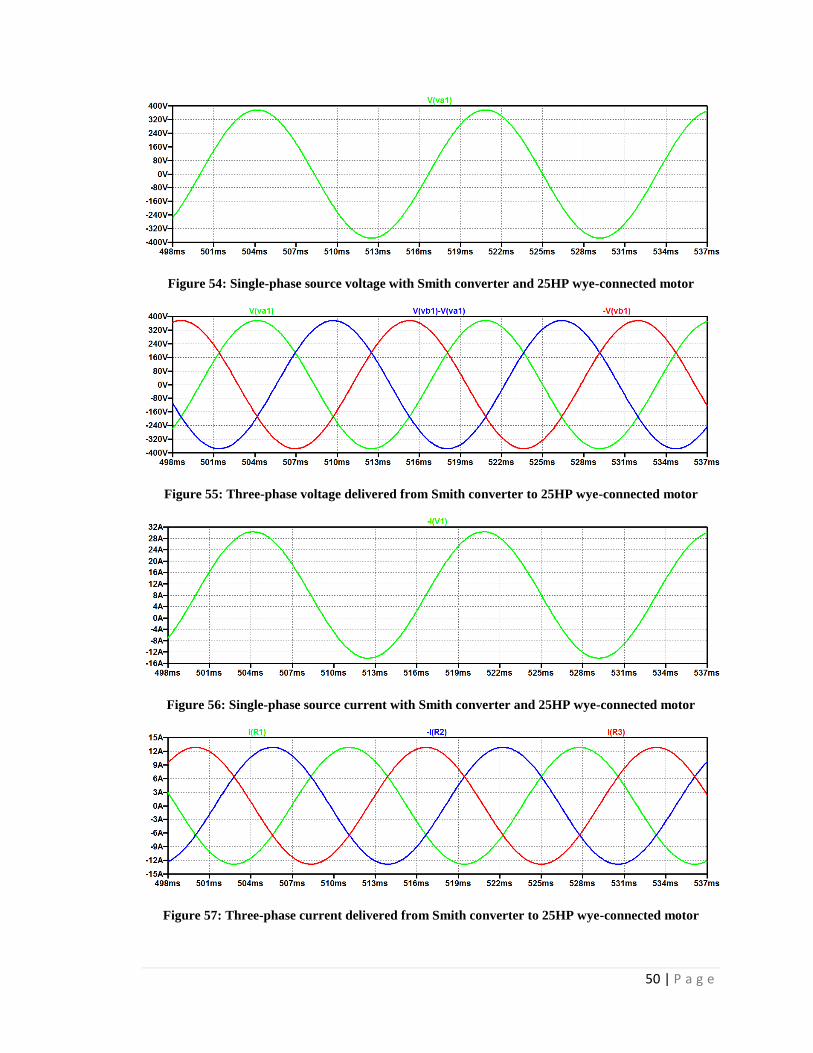
50 | P a g e

Figure 54: Single-phase source voltage with Smith converter and 25HP wye-connected motor

Figure 55: Three-phase voltage delivered from Smith converter to 25HP wye-connected motor

Figure 56: Single-phase source current with Smith converter and 25HP wye-connected motor

Figure 57: Three-phase current delivered from Smith converter to 25HP wye-connected motor

51 | P a g e


converter and the 25HP wye-connected motor. Its amplitude is 22.26A with an offset of

8.11A, increasing the peak current to 30.37A. This is due to the same reason as the other

systems. The current is not initialized to zero by the simulation settings. Therefore, we

will incorporate a varistor into the network to initialize the voltage and the current. This

is shown in Figure 58, below.

Figure 58: LTspice model of Smith converter with 25hp wye-connected motor with varistor



voltage. The addition of the varistor results in the source current waveform shown in

Figure 59 below, and is equivalent to the original waveform but with the reference set at

0A. The amplitude balance and phase shift of the three-phase current in the motor also

remains unaffected.

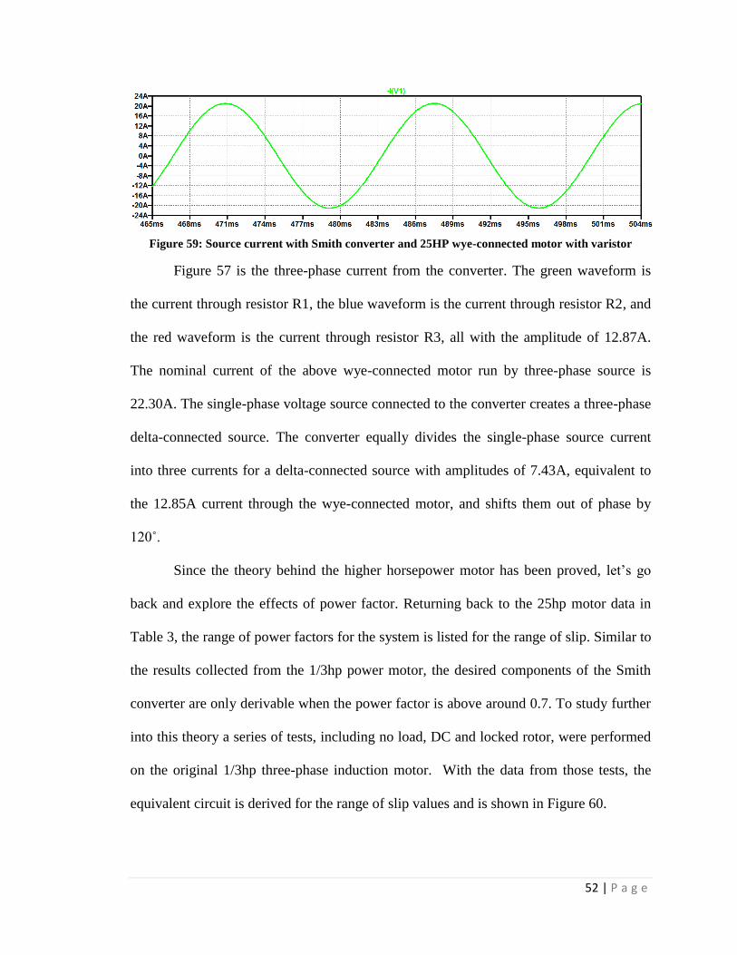
52 | P a g e

Figure 59: Source current with Smith converter and 25HP wye-connected motor with varistor



the red waveform is the current through resistor R3, all with the amplitude of 12.87A.

The nominal current of the above wye-connected motor run by three-phase source is

22.30A. The single-phase voltage source connected to the converter creates a three-phase

delta-connected source. The converter equally divides the single-phase source current

into three currents for a delta-connected source with amplitudes of 7.43A, equivalent to

the 12.85A current through the wye-connected motor, and shifts them out of phase by

120˚.

Since the theory behind the higher horsepower motor has been proved, let’s go

back and explore the effects of power factor. Returning back to the 25hp motor data in

Table 3, the range of power factors for the system is listed for the range of slip. Similar to

the results collected from the 1/3hp power motor, the desired components of the Smith

converter are only derivable when the power factor is above around 0.7. To study further

into this theory a series of tests, including no load, DC and locked rotor, were performed

on the original 1/3hp three-phase induction motor. With the data from those tests, the

equivalent circuit is derived for the range of slip values and is shown in Figure 60.

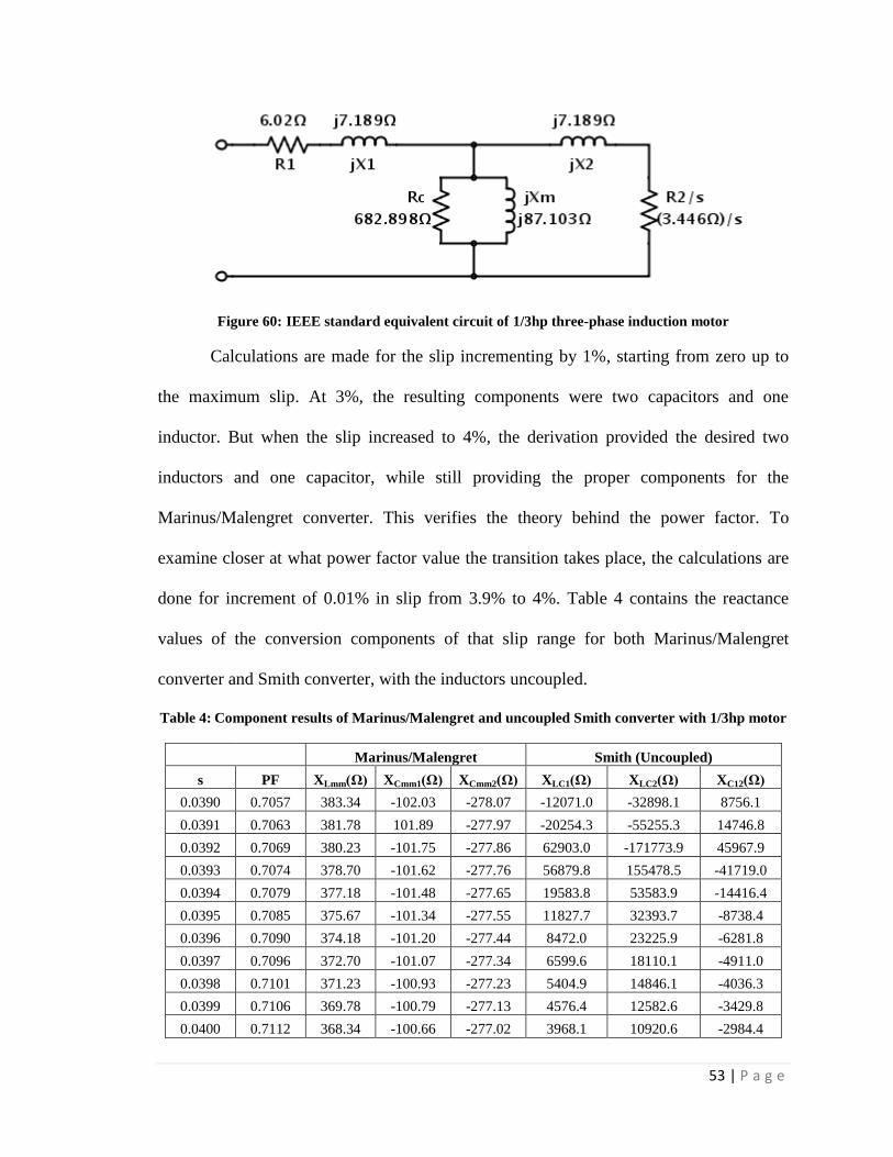
53 | P a g e

Figure 60: IEEE standard equivalent circuit of 1/3hp three-phase induction motor

Calculations are made for the slip incrementing by 1%, starting from zero up to

the maximum slip. At 3%, the resulting components were two capacitors and one

inductor. But when the slip increased to 4%, the derivation provided the desired two

inductors and one capacitor, while still providing the proper components for the

Marinus/Malengret converter. This verifies the theory behind the power factor. To

examine closer at what power factor value the transition takes place, the calculations are

done for increment of 0.01% in slip from 3.9% to 4%. Table 4 contains the reactance

values of the conversion components of that slip range for both Marinus/Malengret

converter and Smith converter, with the inductors uncoupled.

Table 4: Component results of Marinus/Malengret and uncoupled Smith converter with 1/3hp motor

Marinus/Malengret Smith (Uncoupled)

s PF XLmm(Ω) XCmm1(Ω) XCmm2(Ω) XLC1(Ω) XLC2(Ω) XC12(Ω)

0.0390 0.7057 383.34 -102.03 -278.07 -12071.0 -32898.1 8756.1

0.0391 0.7063 381.78 101.89 -277.97 -20254.3 -55255.3 14746.8

0.0392 0.7069 380.23 -101.75 -277.86 62903.0 -171773.9 45967.9

0.0393 0.7074 378.70 -101.62 -277.76 56879.8 155478.5 -41719.0

0.0394 0.7079 377.18 -101.48 -277.65 19583.8 53583.9 -14416.4

0.0395 0.7085 375.67 -101.34 -277.55 11827.7 32393.7 -8738.4

0.0396 0.7090 374.18 -101.20 -277.44 8472.0 23225.9 -6281.8

0.0397 0.7096 372.70 -101.07 -277.34 6599.6 18110.1 -4911.0

0.0398 0.7101 371.23 -100.93 -277.23 5404.9 14846.1 -4036.3

0.0399 0.7106 369.78 -100.79 -277.13 4576.4 12582.6 -3429.8

0.0400 0.7112 368.34 -100.66 -277.02 3968.1 10920.6 -2984.4

54 | P a g e

The transition occurs at a power factor of 0.7074. The component values derived

at that power factor are too large, so the values for a slip of 4% is chosen since the

reactance values of the inductors decrease and still remains under the recommended 5%

slip. Following the same procedure as with the 25hp motor, the inductors are coupled

together and negative mutual inductance is combined with the capacitance to create the

conversion network in Figure 61.

Figure 61: LTspice model of Smith converter with 1/3hp delta-connected motor


converter and the 1/3HP delta-connected motor. This waveform is also the reference


voltage delivered from the converter to the motor. The green waveform is the reference

voltage with a phase of 0˚, the blue waveform is the voltage between the top and middle

line of the system shifted by +120˚, and the red waveform is the voltage between the

middle and bottom line shifted by -120˚, all with the amplitude of 170V. Figure 64

displays the current from the single-phase source driving the Smith converter and the

1/3HP delta-connected motor. Its amplitude is 1.862A with an offset of 0.922A,

increasing the peak current to 2.784A.

55 | P a g e

Figure 62: Single-phase source voltage with Smith converter and 1/3HP delta-connected motor

Figure 63: Three-phase voltage delivered from Smith converter to 1/3HP delta-connected motor

Figure 64: Single-phase source current with Smith converter and 1/3HP delta-connected motor

Figure 65: Three-phase current delivered from Smith converter to 1/3HP delta-connected motor

56 | P a g e

The source current offset is due to the same reason as the other systems. The

current is not initialized to zero by the simulation settings. Therefore, we will incorporate

the varistor into the network to initialize the voltage and the current. This is shown in

Figure 66, below.

Figure 66: LTspice model of Smith converter with 1/3hp delta-connected motor with varistor





0A. The amplitude balance and shift of the three-phase current through the motor also

remains unaffected by the varistor.

Figure 67: Source current with Smith converter and 1/3HP delta-connected motor with varistor

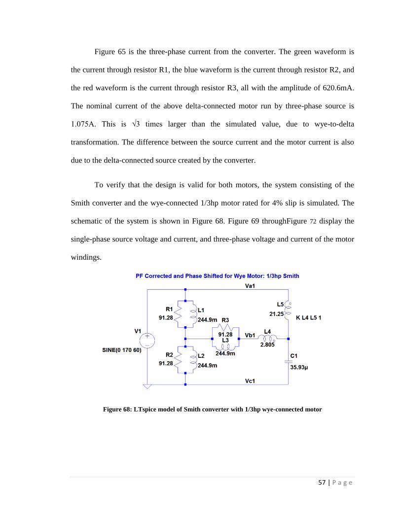
57 | P a g e



the red waveform is the current through resistor R3, all with the amplitude of 620.6mA.

The nominal current of the above delta-connected motor run by three-phase source is

1.075A. This is √3 times larger than the simulated value, due to wye-to-delta

transformation. The difference between the source current and the motor current is also

due to the delta-connected source created by the converter.

To verify that the design is valid for both motors, the system consisting of the

Smith converter and the wye-connected 1/3hp motor rated for 4% slip is simulated. The

schematic of the system is shown in Figure 68. Figure 69 throughFigure 72 display the

single-phase source voltage and current, and three-phase voltage and current of the motor

windings.

Figure 68: LTspice model of Smith converter with 1/3hp wye-connected motor

58 | P a g e

Figure 69: Single-phase source voltage with Smith converter and 1/3HP wye-connected motor

Figure 70: Three-phase voltage delivered from Smith converter to 1/3HP wye-connected motor

Figure 71: Single-phase source current with Smith converter and 1/3HP wye-connected motor

Figure 72: Three-phase current delivered from Smith converter to 1/3HP wye-connected motor

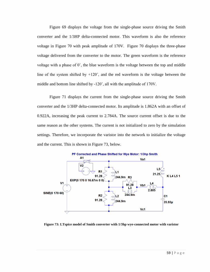
59 | P a g e


converter and the 1/3HP delta-connected motor. This waveform is also the reference


voltage delivered from the converter to the motor. The green waveform is the reference

voltage with a phase of 0˚, the blue waveform is the voltage between the top and middle

line of the system shifted by +120˚, and the red waveform is the voltage between the

middle and bottom line shifted by -120˚, all with the amplitude of 170V.


converter and the 1/3HP delta-connected motor. Its amplitude is 1.862A with an offset of

0.922A, increasing the peak current to 2.784A. The source current offset is due to the

same reason as the other systems. The current is not initialized to zero by the simulation

settings. Therefore, we incorporate the varistor into the network to initialize the voltage

and the current. This is shown in Figure 73, below.

Figure 73: LTspice model of Smith converter with 1/3hp wye-connected motor with varistor

60 | P a g e





0A. The amplitude balance and shift of the three-phase current through the motor also

remains unaffected by the varistor.

Figure 74: Source current with Smith converter and 1/3HP wye-connected motor with varistor

Figure 72 displays the current from the single-phase source. The green waveform

is the current through resistor R1, the blue waveform is the current through resistor R2,

and the red waveform is the current through resistor R3, all with the amplitude of 1.075A.

The nominal current of the above wye-connected motor run by three-phase source is

1.862A. This is √3 times larger than the simulated value, due to wye-to-delta

transformation. The difference between the source current and the motor current is also

due to the delta-connected source created by the converter.

Since the results for both the 1/3hp and 25hp motors provide the desired Smith

converter components for motors operating at a power factor of 0.707 and above, it can

be concluded that the power factor is what controls the outcome of the converter

derivations. Due to the relationship that higher horsepower motors experience higher

power factors, a second conclusion can be made that using a higher horsepower motor is

61 | P a g e

recommended to better achieve the power factor value. Running a smaller horsepower

motor with a larger slip will introduce more current into the system, decreasing the

efficiency and heating up the motor that could eventually damage the system if it is run

for a long period of time. But it is not required to use a larger horsepower motor, since

the Smith converter can be derived using the 1/3hp motor.

62 | P a g e

Chapter 3: Sensitivity Analysis

Now that the derivations have been verified for the Marinus/Malengret and Smith

single to three-phase conversion networks, it is important to look at the sensitivity of each

system. There are two factors that can cause the system to function out of the bounds of

ideality. These factors consist of the variation of the torque within the motor and the

variation of the components within the conversion networks.

3.1 Measurement Procedure

The measurement method used for the sensitivity analysis is a form Error Vector

Magnitude (EVM). EVM is usually used for complex communication systems to measure

modulation accuracy. It considers all of the potential phase and amplitude distortions as

well as noise and provides a single comprehensive measurement figure for determining

the quality of a circuit or product [13]. This study can use the same form of analysis since

we want to measure the phase and amplitude distortions due to variation in the torque of

the motor and the values of the components in the conversion network.

Figure 75: Block diagram of Error Vector Magnitude (EVM) measurement method

V13

V32

V21

V1

V2

V3

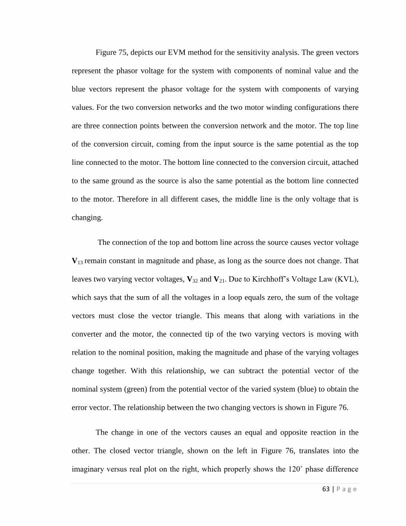
63 | P a g e

Figure 75, depicts our EVM method for the sensitivity analysis. The green vectors

represent the phasor voltage for the system with components of nominal value and the

blue vectors represent the phasor voltage for the system with components of varying

values. For the two conversion networks and the two motor winding configurations there

are three connection points between the conversion network and the motor. The top line

of the conversion circuit, coming from the input source is the same potential as the top

line connected to the motor. The bottom line connected to the conversion circuit, attached

to the same ground as the source is also the same potential as the bottom line connected

to the motor. Therefore in all different cases, the middle line is the only voltage that is

changing.

The connection of the top and bottom line across the source causes vector voltage

V13 remain constant in magnitude and phase, as long as the source does not change. That

leaves two varying vector voltages, V32 and V21. Due to Kirchhoff’s Voltage Law (KVL),

which says that the sum of all the voltages in a loop equals zero, the sum of the voltage

vectors must close the vector triangle. This means that along with variations in the

converter and the motor, the connected tip of the two varying vectors is moving with

relation to the nominal position, making the magnitude and phase of the varying voltages

change together. With this relationship, we can subtract the potential vector of the

nominal system (green) from the potential vector of the varied system (blue) to obtain the

error vector. The relationship between the two changing vectors is shown in Figure 76.

The change in one of the vectors causes an equal and opposite reaction in the

other. The closed vector triangle, shown on the left in Figure 76, translates into the

imaginary versus real plot on the right, which properly shows the 120˚ phase difference

64 | P a g e

between each voltage and the error relationship. This error vector causes V32 to increase

in magnitude and phase, and equally decrease V21 in magnitude and phase.

Figure 76: Closed triangle vector form to phasor plot representation of three-phase voltage

This method of measurement is a good technique for lab experimentation on

systems of this nature, since the connections of the motor windings and conversion

circuitry would be enclosed and would not always be easily accessible. As long as there

are connection points, the voltage can always be probed, making this method easy to

perform. To verify the accuracy of this measurement method, analysis will also be done

on the current through the windings.

3.2 Torque Variation

The first set of sensitivity analysis is done on the torque variation of the motor. As

discussed previously in Section 1.1.1, when modeling the resistance and inductance of

the motor windings in parallel, the change in torque can be modeled as the change in

resistance within the winding. From the results in Figure 13, the inductance value stays

relatively the same and the resistance decreases as the torque increases. Therefore, we

can model and simulate the sensitivity to torque variation as the change in resistance of

the motor windings using LTspice. A variation of ±15% was chosen to analyze the

V32

V21

V13

V32

V13

V21

65 | P a g e

characteristics of the system with the torque varying around the operating point of the

motor. Due to the extrapolation of data to acquire the winding resistance there is some

margin of difference for the ±15% torque variation by ±0.5%.

3.2.1 Induction Motor with Marinus/Malengret Converter

Figure 77 displays the result for varying the torque by ±15% for both the wye and

delta-connected motors. The voltage vectors resulting in the negative quadrant are due to

the +15% change in torque and the vectors in the positive quadrant are due to the -15%

change in torque. The relationship between the change in error vector as the torque

shows that the system is more sensitive to the decrease in torque versus the increase. The

rectangular form dimensions of the vector are in terms of percentage of voltage, therefore

the polar form of the vector has a magnitude of percent peak nominal voltage and the

phase error in degrees.

Figure 77: Voltage error vector results of ±15% torque variation on motor with MM converter

-15

-10

-5

0

5

10

15

20

-0.04 -0.03 -0.02 -0.01 0 0.01 0.02 0.03

Ima

gin

ary

(%

)

Real (%)

Voltage Error Vectors: Torque Variation with Marinus/Malengret

Converter

Wye-Connected

Delta_Connected

66 | P a g e

The variation in toque causes the same error vector results for both the wye and

delta-connected motors. The magnitude of the error voltage vector changes by roughly

15% and 13% for the -15% and +15% changes in torque, respectively. Both error vectors

move along the imaginary axis and deviate from normal by 0.1˚. This means that the

connecting point of V21 and V32 changes vertically together and will cause the

magnitudes and phase to change at the same rate, with some difference due to the slight

phase difference of the error vector caused by the phase converter. This relationship is

shown in Figure 78.

Figure 78: Closed three-phase vector triangle (green) with error vectors (red)

To further examine the effects of torque variation on both motors for the

Marinus/Malengret converter, below are the figures that display the variation of the

current in the time domain. Figure 79 throughFigure 82 display the nominal current

waveforms in a delta-connected motor from a three-phase source for the converter at

nominal, +15% and -15% torque.

V13

V32 V21

67 | P a g e

Figure 79: Three-phase current of 1/3HP delta-connected motor driven by three-phase source

Figure 80: Three-phase current from MM converter to 1/3HP delta-connected motor at nominal

torque

Figure 81: Three-phase current from MM converter to 1/3HP delta-connected motor at +15% torque

Figure 82: Three-phase current from MM converter to 1/3HP delta-connected motor at -15% torque

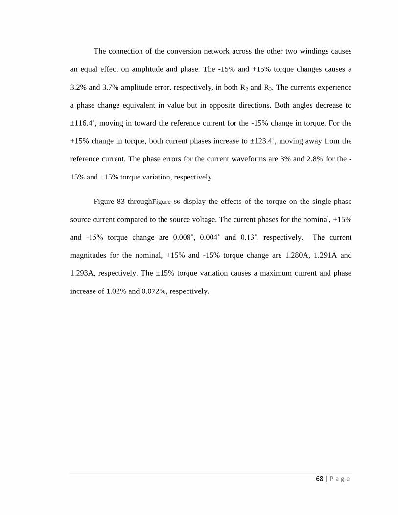
68 | P a g e

The connection of the conversion network across the other two windings causes

an equal effect on amplitude and phase. The -15% and +15% torque changes causes a

3.2% and 3.7% amplitude error, respectively, in both R2 and R3. The currents experience

a phase change equivalent in value but in opposite directions. Both angles decrease to

±116.4˚, moving in toward the reference current for the -15% change in torque. For the

+15% change in torque, both current phases increase to ±123.4˚, moving away from the

reference current. The phase errors for the current waveforms are 3% and 2.8% for the -

15% and +15% torque variation, respectively.

Figure 83 throughFigure 86 display the effects of the torque on the single-phase

source current compared to the source voltage. The current phases for the nominal, +15%

and -15% torque change are 0.008˚, 0.004˚ and 0.13˚, respectively. The current

magnitudes for the nominal, +15% and -15% torque change are 1.280A, 1.291A and

1.293A, respectively. The ±15% torque variation causes a maximum current and phase

increase of 1.02% and 0.072%, respectively.

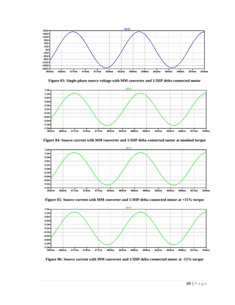
69 | P a g e

Figure 83: Single-phase source voltage with MM converter and 1/3HP delta-connected motor

Figure 84: Source current with MM converter and 1/3HP delta-connected motor at nominal torque

Figure 85: Source current with MM converter and 1/3HP delta-connected motor at +15% torque

Figure 86: Source current with MM converter and 1/3HP delta-connected motor at -15% torque

70 | P a g e

Figure 87: Three-phase current of 1/3HP wye-connected motor driven by three-phase source

Figure 88: Three-phase current from MM converter to 1/3HP wye-connected motor at nominal

torque

Figure 89: Three-phase current from MM converter to 1/3HP wye-connected motor at +15% torque

Figure 90: Three-phase current from MM converter to 1/3HP wye-connected motor at -15% torque

71 | P a g e

Figure 87 displays the current in the 1/3HP wye-connected motor operating from

a three-phase source, each waveform resulting in a peak value of 1.28A. Figure 88

displays the current at nominal torque, with the same peak values of 738.9mA. Figure 89

displays the current at +15% change in torque with peak values of about 818.0mA for R1

and R2, and 738.9mA for R3. Figure 90 displays the current at -15% change in torque

with peak values of about 665.7mA for both R1 and R2, and 738.9mA for R3. The current

through R3 remains the same no matter the change in torque. The connection of R3 to the

conversion network holds the value steady as it causes the rest of the circuit that is

parallel to it to vary. This could be due to an H-bridge relationship


an equal effect on the amplitude and phase. The -15% and +15% torque changes cause a

9.9% and 10.7% amplitude error, respectively, in both R1 and R2. The currents experience

a phase change equivalent in values but in opposite directions. Both angles decrease to

±116.8˚ moving in towards the reference current for the -15% change in torque. For the

+15% change in torque, both current phases increase to ±123.7˚, moving away from the

reference current. The phase errors for the current waveforms are 2.7% and 3.1% for the -

15% and +15% torque variation, respectively.

Figure 91 through Figure 94 display the effects of the torque on the single-phase

source current compared to the source voltage. The current phases for the nominal, +15%

and -15% torque change are 0.008˚, 0.004˚ and 0.13˚, respectively. The current

magnitudes for the nominal, +15% and -15% torque change are 1.280A, 1.290A and

1.293. The ±15% torque variation causes a maximum current and phase increase of

1.02% and 0.072%, respectively, like in the delta-connected motor.

72 | P a g e

Figure 91: Single-phase source voltage with MM converter and 1/3HP wye-connected motor

Figure 92: Source current with MM converter and 1/3HP wye-connected motor at nominal torque

Figure 93: Source current with MM converter and 1/3HP wye-connected motor at +15% torque

Figure 94: Source current with MM converter and 1/3HP wye-connected motor at -15% torque

73 | P a g e

3.2.2 Induction Motor with Smith Converter

Figure 95 displays the result for the torque variation of the wye and delta-

connected motors, represented by the variation of the motor winding resistance, when

connected to the Smith converter. The voltage vectors resulting in the negative quadrant

are due to the +15% change torque and the vectors in the positive quadrant are due to the

-15% change in torque. The relationship between the change in error vector as the torque

shows that the system is more sensitive to the decrease in torque versus the increase. The

rectangular form dimensions of the vector are in terms of percent voltage, therefore the

polar form of the vector have a magnitude of percent peak nominal voltage and the phase

error in degrees.

Figure 95: Voltage error vector results from ±15% torque variation on wye and delta-connected

induction motor with Smith converter

The error voltage magnitudes change by approximately 13.6% and 11.2% for the

+15% and -15% torque change, respectively. The error vectors move along the imaginary

axis and deviate from the normal by 0.02˚ and 0.04˚ for the wye and delta-connected

-15

-10

-5

0

5

10

15

-0.01 -0.008 -0.006 -0.004 -0.002 0 0.002 0.004 0.006 0.008

Ima

gin

ary

(%

)

Real (%)

Voltage Error Vectors: Torque Variation with Smith Converter

Wye-Connected

Delta-Connected

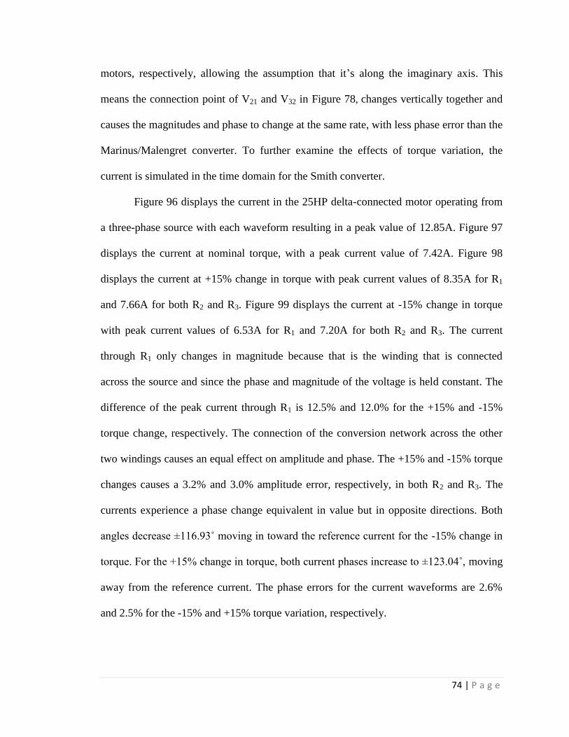
74 | P a g e

motors, respectively, allowing the assumption that it’s along the imaginary axis. This

means the connection point of V21 and V32 in Figure 78, changes vertically together and

causes the magnitudes and phase to change at the same rate, with less phase error than the

Marinus/Malengret converter. To further examine the effects of torque variation, the

current is simulated in the time domain for the Smith converter.

Figure 96 displays the current in the 25HP delta-connected motor operating from

a three-phase source with each waveform resulting in a peak value of 12.85A. Figure 97

displays the current at nominal torque, with a peak current value of 7.42A. Figure 98

displays the current at +15% change in torque with peak current values of 8.35A for R1

and 7.66A for both R2 and R3. Figure 99 displays the current at -15% change in torque

with peak current values of 6.53A for R1 and 7.20A for both R2 and R3. The current

through R1 only changes in magnitude because that is the winding that is connected

across the source and since the phase and magnitude of the voltage is held constant. The

difference of the peak current through R1 is 12.5% and 12.0% for the +15% and -15%

torque change, respectively. The connection of the conversion network across the other

two windings causes an equal effect on amplitude and phase. The +15% and -15% torque

changes causes a 3.2% and 3.0% amplitude error, respectively, in both R2 and R3. The

currents experience a phase change equivalent in value but in opposite directions. Both

angles decrease ±116.93˚ moving in toward the reference current for the -15% change in

torque. For the +15% change in torque, both current phases increase to ±123.04˚, moving

away from the reference current. The phase errors for the current waveforms are 2.6%

and 2.5% for the -15% and +15% torque variation, respectively.

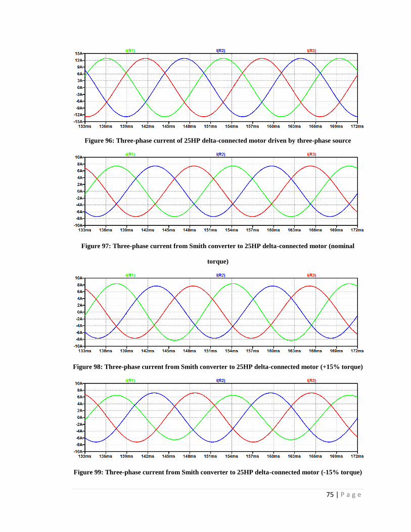
75 | P a g e

Figure 96: Three-phase current of 25HP delta-connected motor driven by three-phase source

Figure 97: Three-phase current from Smith converter to 25HP delta-connected motor (nominal

torque)

Figure 98: Three-phase current from Smith converter to 25HP delta-connected motor (+15% torque)

Figure 99: Three-phase current from Smith converter to 25HP delta-connected motor (-15% torque)

76 | P a g e

Figure 100: Single-phase source voltage with Smith converter and 25HP delta-connected motor

Figure 101: Source current with Smith converter and 25HP delta-connected motor at nominal torque

Figure 102: Source current with Smith converter and 25HP delta-connected motor at +15% torque

Figure 103: Source current with Smith converter and 25HP delta-connected motor at -15% torque

77 | P a g e

Figure 100 throughFigure 103 display the effects of the torque on the single-phase

source current compared to the source voltage. Due to the offset issue previously

discovered, a varistor added to the network to gradually increase the source to initialize

the voltage and current to zero resulting in the elimination of the offset. The current

phases for the nominal, +15% and -15% torque change are 0˚, 0˚ and 0.002˚, respectively.

The current magnitudes for the nominal, +15% and -15% torque change are 22.26A,

22.39A and 22.41A, respectively. The ±15% torque variation causes a maximum current

and phase increase of 0.76% and 0.001%, respectively.

Figure 104 displays the current in the 25HP wye-connected motor operating from

a three-phase source with each waveform resulting in a peak value of 22.26A. Figure 105

displays the current at nominal torque, with the peak current of 12.85A. Figure 106

displays the current at +15% change in torque with peak current values of about 14.09A

for both R1 and R2, and 12.85A for R3. Figure 107 displays the current at -15% change in

torque with peak current values of about 11.71A for R1 and R2, and 12.85A for R3. The

current through R3 remains the same no matter the change in torque.


an equal effect on the amplitude and phase. The -15% and +15% torque changes causes

an 8.9% and 9.6% amplitude error, respectively, in both R1 and R2. The currents

experience a phase change equivalent in values but in opposite directions. Both angles

decrease to ±117.13˚ moving in towards the reference current for the -15% change in

torque. For the +15% change in torque, both current phases increase to ±123.26˚, moving

away from the reference current. The phase errors for the current waveforms are 2.3%

and 2.7% for the -15% and +15% torque variation, respectively.

78 | P a g e

Figure 104: Three-phase current of 25HP wye-connected motor driven by three-phase source

Figure 105: Three-phase current from Smith converter to 25HP wye-connected motor (nominal

torque)

Figure 106: Three-phase current from Smith converter to 25HP wye-connected motor (+15% torque)

Figure 107: Three-phase current from Smith converter to 25HP wye-connected motor (-15% torque)

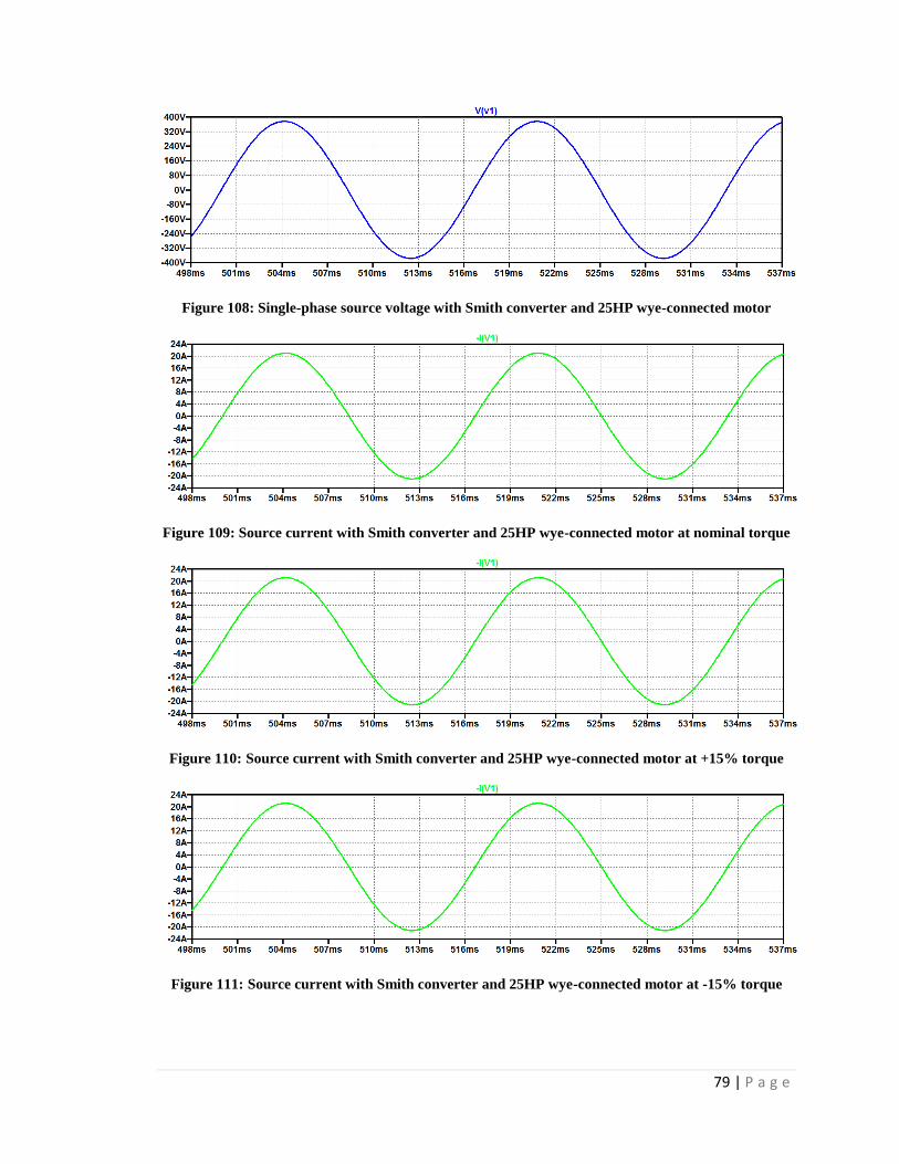
79 | P a g e

Figure 108: Single-phase source voltage with Smith converter and 25HP wye-connected motor

Figure 109: Source current with Smith converter and 25HP wye-connected motor at nominal torque

Figure 110: Source current with Smith converter and 25HP wye-connected motor at +15% torque

Figure 111: Source current with Smith converter and 25HP wye-connected motor at -15% torque

80 | P a g e

Figure 108 through Figure 111 display the effects of the torque on the single-phase

source current compared to the source voltage. Due to the offset issue previously

discovered, a varistor added to the network to gradually increase the source to initialize

the voltage and current to zero resulting in the elimination of the offset. The current

phases for the nominal, +15% and -15% torque change are 0˚, 0˚ and 0.002˚, respectively.

The current magnitudes for the nominal, +15% and -15% torque change are 22.26A,

22.39A and 22.41A, respectively. The ±15% torque variation causes a maximum current

and phase increase of 0.76% and 0.001%, respectively, like with the delta-connected

motor.

Overall, the variation in torque doesn’t have too much effect on the phase of each

system. With the ±15% change in torque, two of the three phases change between 2% and

3%. The converter that experienced the smallest phase change was the Smith converter.

The wye-connected motor experiences amplitude variation for two of the three phases,

whereas the delta-connected motor network experiences amplitude variation in all three

but mostly in only one. The input source current amplitude doesn’t vary more 0.46% and

0.59% for the Marinus/Malnegret and Smith converters, respectively. The phase changes

by 0.002% and 0.14%. Therefore, the change in source current is minimal.

As a total, the systems are more sensitive to the decrease in torque versus the

increase. This is due to the stability of the conversion network. The single to three-phase

converters are designed for a certain resistance of the motor winding and when the

resistance is increased in the parallel winding, making the system more inductive and

capacitive, larger transients are introduced. When analyzing the data for both motors, the

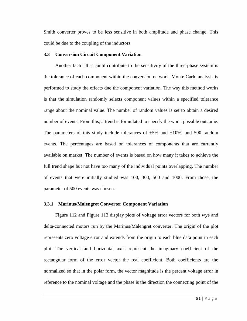
81 | P a g e

Smith converter proves to be less sensitive in both amplitude and phase change. This

could be due to the coupling of the inductors.

3.3 Conversion Circuit Component Variation

Another factor that could contribute to the sensitivity of the three-phase system is

the tolerance of each component within the conversion network. Monte Carlo analysis is

performed to study the effects due the component variation. The way this method works

is that the simulation randomly selects component values within a specified tolerance

range about the nominal value. The number of random values is set to obtain a desired

number of events. From this, a trend is formulated to specify the worst possible outcome.

The parameters of this study include tolerances of ±5% and ±10%, and 500 random

events. The percentages are based on tolerances of components that are currently

available on market. The number of events is based on how many it takes to achieve the

full trend shape but not have too many of the individual points overlapping. The number

of events that were initially studied was 100, 300, 500 and 1000. From those, the

parameter of 500 events was chosen.

3.3.1 Marinus/Malengret Converter Component Variation

Figure 112 and Figure 113 display plots of voltage error vectors for both wye and

delta-connected motors run by the Marinus/Malengret converter. The origin of the plot

represents zero voltage error and extends from the origin to each blue data point in each

plot. The vertical and horizontal axes represent the imaginary coefficient of the

rectangular form of the error vector the real coefficient. Both coefficients are the

normalized so that in the polar form, the vector magnitude is the percent voltage error in

reference to the nominal voltage and the phase is the direction the connecting point of the

82 | P a g e

two varying vectors is moving, like in Figure 78 from the previous section. Each plot

exhibits close to a linear relationship through the origin of the real-imaginary axis. The

top right quadrant displays the +5% and +10% component variation whereas the bottom

left quadrant displays the -5% and -10% component variation.

When the wye and delta-connected motors are run by the Marinus/Malangret

converter, the voltage error is evenly distributed along an angle of about 15˚ and 205˚

from the origin for both component variations. The error vectors can experience a

direction of any angle but due to the trend in data, it is more likely for the vector to point

along the 15˚ and 205˚ direction to the opposite ends of the rectangular shaped plot trend.

These vectors represent the maximum error of 14% and 28% magnitude voltage and can

rotate to the outer most corners by ±5˚ and ±10˚, with a ±1% and ±2% change in

magnitude for the ±5% and ±10% component variation, respectively. The width of the

rectangular trend is approximately 2% and 4% magnitude voltage for ±5% and ±10%

component variation, respectively.

The vectors that formulate around the origin of the plot cause less of an error

since the magnitude is less that 5% magnitude voltage even though the angle is varying

between 0˚ and 360˚. In referencing Figure 78, we can visualize that the small magnitude

of the error vector rotating around the origin in a circular motion will cause a small error

in the two voltage vectors V32 and V21. The vectors that reach outer most corners of the

trend will cause a larger error of V32 and V21 due to the larger vector magnitude.

83 | P a g e

Figure 112: Error vector plot of ±5%/ ±10% component variation Monte Carlo in Marinus/Malengret converter with delta-connected motor

Figure 113: Error vector plot of ±5%/±10% component variation Monte Carlo in Marinus/Malengret converter with wye-connected motor

-12

-8

-4

0

4

8

12

-30 -25 -20 -15 -10 -5 0 5 10 15 20 25 30 35

Imag

inar

y (%

)

Real (%)

Voltage Error Vectors (Delta): MM Component Variation ±5%

-12

-8

-4

0

4

8

12

-30 -25 -20 -15 -10 -5 0 5 10 15 20 25 30 35

Imag

inar

y (%

)

Real (%)

Voltage Error Vectors (Delta): MM Component Variation ±10%

-12

-8

-4

0

4

8

12

-30 -25 -20 -15 -10 -5 0 5 10 15 20 25 30 35

Imag

inar

y (%

)

Real (%)

Voltage Error Vectors (Wye): MM Component Variation ±5%

-12

-8

-4

0

4

8

12

-30 -25 -20 -15 -10 -5 0 5 10 15 20 25 30 35

Imag

inar

y (%

)

Real (%)

Voltage Error Vectors (Wye): MM Component Variation ±10%

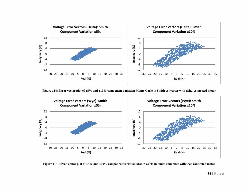
84 | P a g e

Figure 114: Error vector plot of ±5% and ±10% component variation Monte Carlo in Smith converter with delta-connected motor

Figure 115: Error vector plot of ±5% and ±10% component variation Monte Carlo in Smith converter with wye-connected motor

-12

-8

-4

0

4

8

12

-30 -25 -20 -15 -10 -5 0 5 10 15 20 25 30 35

Imag

inar

y (%

)

Real (%)

Voltage Error Vectors (Delta): Smith Component Variation ±5%

-12

-8

-4

0

4

8

12

-30 -25 -20 -15 -10 -5 0 5 10 15 20 25 30 35

Imag

inar

y (%

)

Real (%)

Voltage Error Vectors (Delta): Smith Component Variation ±10%

-12

-8

-4

0

4

8

12

-30 -25 -20 -15 -10 -5 0 5 10 15 20 25 30 35

Imag

inar

y (%

)

Real (%)

Voltage Error Vectors (Wye): Smith Component Variation ±5%

-12

-8

-4

0

4

8

12

-30 -25 -20 -15 -10 -5 0 5 10 15 20 25 30 35

Imag

inar

y (%

)

Real (%)

Voltage Error Vectors (Wye): Smith Component Variation ±10%

85 | P a g e

3.3.2 Smith Converter Component Variation

Figure 114 and Figure 115 display the data collected for both wye and delta-

connected motors run by the Smith converter. The data is displayed using the same

parameters as the Marinus/Malengret component variation data. Like the previous

section, the top right quadrant displays the +5% and +10% component variation whereas

the bottom left quadrant displays the -5% and -10% component variation. The vector

magnitude is the percent voltage error in reference to the nominal voltage and the phase

is the direction the connecting point of the two varying vectors is moving, like in Figure

78.

When the wye and delta-connected motors are run by the Smith converter, the

voltage error is evenly distributed along an angle of about 25˚ and 210˚ from the origin

for both component variations. The error vectors can experience a direction of any angle

but due to the trend in data, it is more likely for the vector to point along the 25˚ and 210˚

direction to the opposite ends of the rectangular shaped plot trend. These vectors

represent the percent voltage error along the trend line of 10% and 18% magnitude

voltage and can rotate to the outer most corners by ±13˚ for both ±5% and ±10%

component variation, with a ±5% and ±7% change in magnitude, respectively. The width

of the rectangular trend is approximately 4% and 8% magnitude voltage for ±5% and

±10% component variation, respectively.

Like the previous system, the vectors that formulate around the origin of the plot

cause less of an error since the magnitude is less that 5% magnitude voltage even though

the angle is varying between 0˚ and 360˚. In referencing Figure 78, we can visualize that

the small magnitude of the error vector rotating around the origin in a circular motion

86 | P a g e

will cause a small error in the two voltage vectors V32 and V21. The vectors that reach

outer most corners of the trend will cause a larger error of V32 and V21 due to the larger

vector magnitude.

The results of this testing concludes an overall trend that the component variation

causes an even trade of magnitude and phase of the two branch voltages. As V21

decreases in magnitude and phase, V32 will increase as a result. If V21 increases in

magnitude and phase, then V32 will decrease. There are some instances where the error

voltage vectors are along the imaginary axis causing an equal change in magnitude and

phase in V21 and V32, but those occurrences are less likely to happen.

87 | P a g e

Chapter 4: Additional Motor Configuration

There are a few similarities and differences between the three conversion

networks and their connections to the motors and the source. From the top level

perspective, the Marinus/Malengret and Smith converters consist of three connections,

shown in Figure 116. Two of the three connections are across the source so the potential

of those lines remain constant as long as the source voltage remains constant. These two

lines also connect to the motor, meaning there is only one line between the converter and

the motor that is varying. The three-phase voltage comes from measuring between the

lines meaning that the input voltage to the motor is line-to-line. Both wye and delta-

connected motors can run off of this converted power.

Figure 116: Block diagram of Marinus/Malengret and Smith converter connection to source and

motor

Figure 117 displays the top level diagram for the Cal Poly converter and induction

motor connection. The Cal Poly converter consists of four connection lines, with two

connected across the source also leading to the motor like in the previous system. This

means that there are two varying voltages between the converter and the motor. The

88 | P a g e

bottom of the four lines is connected to a neutral potential and the other three lines are

measured with reference to that line. This means that the input voltage of the motor is

phase voltage and line current. The only motor that can utilize the four connections of the

converter is the wye-connected motor. For wye-connected motors, line current is √3

times larger than phase current allowing the converter to supply more power. This means

that the Cal Poly converter can provide higher current for larger loads.

Figure 117: Block diagram of Cal Poly converter connection to source and motor

The observation of the four lines leading from the Cal Poly converter to the motor

introduced a theory of a possible third motor configuration. If we take a delta connected

motor and disconnect two of the windings, it creates an open-delta configuration as

shown in Figure 118. This creates a motor that also consists of four winding connections

like the wye-connected motor.

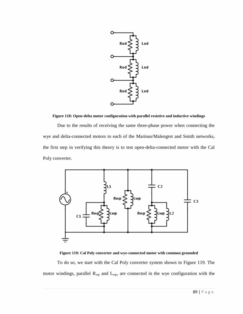
89 | P a g e

Figure 118: Open-delta motor configuration with parallel resistive and inductive windings

Due to the results of receiving the same three-phase power when connecting the

wye and delta-connected motors to each of the Marinus/Malengret and Smith networks,

the first step in verifying this theory is to test open-delta-connected motor with the Cal

Poly converter.

Figure 119: Cal Poly converter and wye-connected motor with common grounded

To do so, we start with the Cal Poly converter system shown in Figure 119. The

motor windings, parallel Rwp and Lwp, are connected in the wye configuration with the

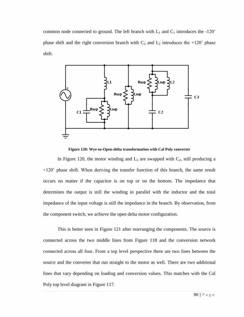
90 | P a g e

common node connected to ground. The left branch with L1 and C1 introduces the -120˚

phase shift and the right conversion branch with C2 and L2 introduces the +120˚ phase

shift.

Figure 120: Wye-to-Open-delta transformation with Cal Poly converter

In Figure 120, the motor winding and L2 are swapped with C2, still producing a

+120˚ phase shift. When deriving the transfer function of this branch, the same result

occurs no matter if the capacitor is on top or on the bottom. The impedance that

determines the output is still the winding in parallel with the inductor and the total

impedance of the input voltage is still the impedance in the branch. By observation, from

the component switch, we achieve the open delta motor configuration.

This is better seen in Figure 121 after rearranging the components. The source is

connected across the two middle lines from Figure 118 and the conversion network

connected across all four. From a top level perspective there are two lines between the

source and the converter that run straight to the motor as well. There are two additional

lines that vary depending on loading and conversion values. This matches with the Cal

Poly top level diagram in Figure 117.

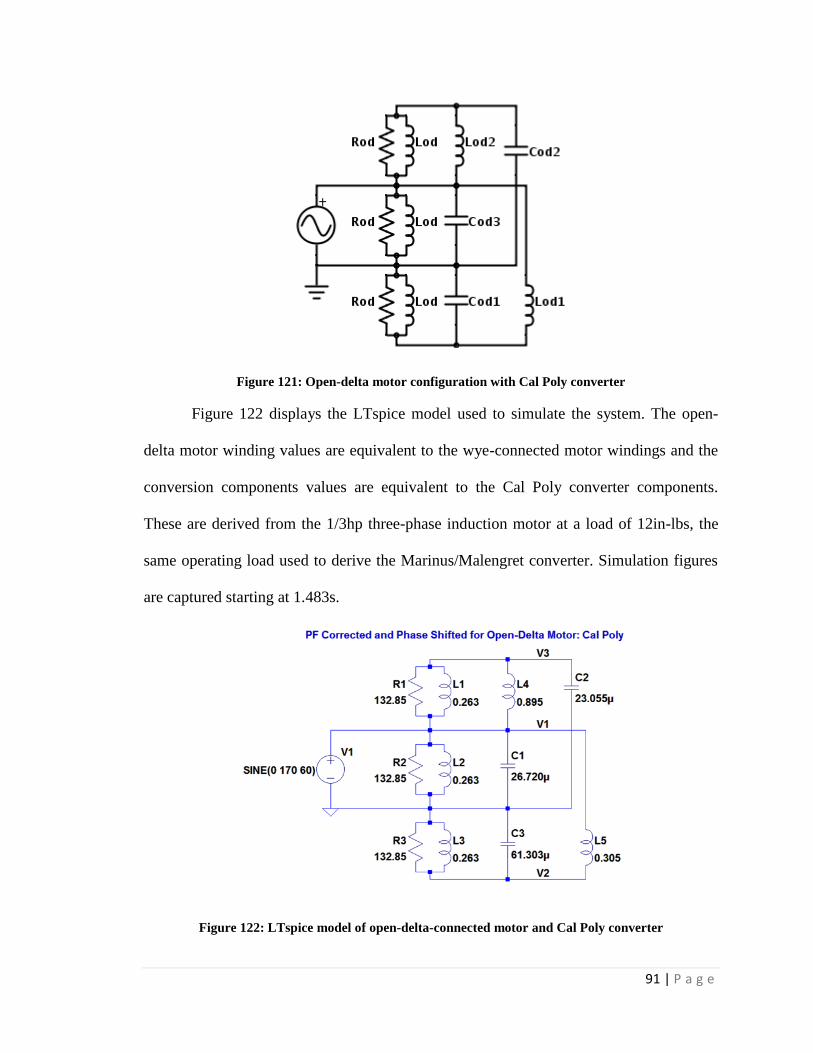
91 | P a g e

Figure 121: Open-delta motor configuration with Cal Poly converter

Figure 122 displays the LTspice model used to simulate the system. The open-

delta motor winding values are equivalent to the wye-connected motor windings and the

conversion components values are equivalent to the Cal Poly converter components.

These are derived from the 1/3hp three-phase induction motor at a load of 12in-lbs, the

same operating load used to derive the Marinus/Malengret converter. Simulation figures

are captured starting at 1.483s.

Figure 122: LTspice model of open-delta-connected motor and Cal Poly converter

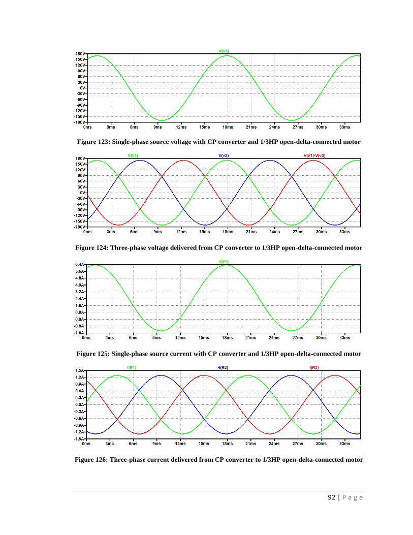
92 | P a g e

Figure 123: Single-phase source voltage with CP converter and 1/3HP open-delta-connected motor

Figure 124: Three-phase voltage delivered from CP converter to 1/3HP open-delta-connected motor

Figure 125: Single-phase source current with CP converter and 1/3HP open-delta-connected motor

Figure 126: Three-phase current delivered from CP converter to 1/3HP open-delta-connected motor

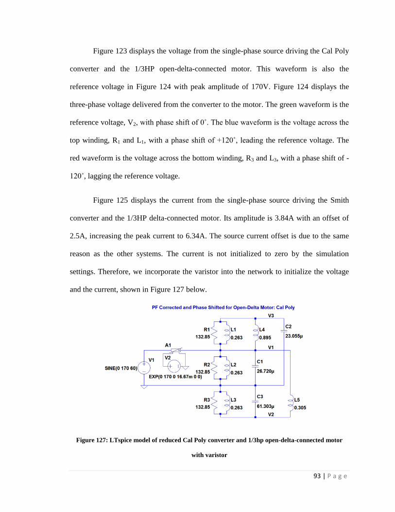
93 | P a g e

Figure 123 displays the voltage from the single-phase source driving the Cal Poly

converter and the 1/3HP open-delta-connected motor. This waveform is also the

reference voltage in Figure 124 with peak amplitude of 170V. Figure 124 displays the

three-phase voltage delivered from the converter to the motor. The green waveform is the

reference voltage, V2, with phase shift of 0˚. The blue waveform is the voltage across the

top winding, R1 and L1, with a phase shift of +120˚, leading the reference voltage. The

red waveform is the voltage across the bottom winding, R3 and L3, with a phase shift of -

120˚, lagging the reference voltage.


converter and the 1/3HP delta-connected motor. Its amplitude is 3.84A with an offset of

2.5A, increasing the peak current to 6.34A. The source current offset is due to the same

reason as the other systems. The current is not initialized to zero by the simulation

settings. Therefore, we incorporate the varistor into the network to initialize the voltage

and the current, shown in Figure 127 below.

Figure 127: LTspice model of reduced Cal Poly converter and 1/3hp open-delta-connected motor

with varistor

94 | P a g e



voltage. The result of the addition of the varistor is shown in Figure 128 below,

displaying the original source current but with the reference set at 0A. The amplitude

balance and shift of the three-phase current through the motor will also remain unaffected

by the varistor.

Figure 128: Source current with CP converter and 1/3HP OD-connected motor with varistor

Figure 126 is the simulation results of the current going through resistance of the

windings from Figure 122. The green, blue and red waveforms are the current flowing

through resistors R1, R2 and R3, respectively. The peak value for each current is 1.28A

which is 1/3 the source current. This is because the converter evenly distributes the

single-phase source current into three currents of amplitude 1.28A, all out of phase by

120˚.

95 | P a g e

Figure 129: Three-phase current of 1/3HP open-delta-connected motor driven by three-phase source

Figure 130: Three-phase current from CP converter to 1/3HP OD-connected motor at nominal

torque

Figure 131: Three-phase current from CP converter to 1/3HP OD-connected motor at +15% torque

Figure 132: Three-phase current from CP converter to 1/3HP OD-connected motor at -15% torque

96 | P a g e

Next is the torque variation analysis for the system. Figure 130 represents the

current at nominal torque, with a peak current value of 1.28A. The Figure 131 represents

the current at +15% change in torque with peak current values of 1.32A for R1 and R3,

and 1.46A for both R2. Figure 132 represents the current at -15% change in torque with

peak current values of 1.23A for R1 and R3, and 1.11A for R2. The current through R2

only changes in magnitude because of the connection across the constant source. The

difference of the peak current through R2 is 14.1% and 13.2% for the +15% and -15%

torque change, respectively.


approximately an equal effect on amplitude and phase. The +15% and -15% torque

change causes a 3.9% and 3.1% amplitude error, respectively, for both R1 and R3. Both

angles decrease approximately ±116.8˚ moving in toward the reference current for the

+15% change in torque. For the -15% change in torque, both current phases increase to

approximately ±123.6˚, moving away from the reference current. The phase error for the

current waveforms are 2.6% and 3.0% for the +15% and -15% torque variation,

respectively.

The amplitude and phase change for R1 and R3 are comparable to the

Marinus/Malengret and Smith converters with the wye and delta-connected motors. The

amplitude change of current through R2 is the highest out of all three making this system

the most sensitive to torque variation.

97 | P a g e

Chapter 5: Applications

In attempts to test these conversion networks, the systems experienced large

transients at the start-up of the motor. This is because at start-up there exists little to no

resistance within the winding, only inductance. The reduction in resistance causes the

transients of the system to spike and can cause damage to the conversion components and

the motor. To be able to use the converters, a start-up network must be incorporated. One

suggestion is to add resistance into the system so the conversion network can “see” the

winding full load at which it is designed to operate and then to remove it when the load of

the winding is high enough to not cause a spike in the voltage and current. Two ways this

can be achieved is by adding resistors in series with the motor lines or in parallel with

switch relays to either short them out or remove them from the system when start-up is

done.

There are a few details to pay attention to in the design of the start-up network.

First being the efficiency of the method. It should be analyzed as to attempt to not

counteract the efficiency of the converter. If the start-up network would be used for a

short period of time, there shouldn’t be too much of a negative contribution. If the

application requires frequent start-ups and introduces the network for longer periods of

time, a start-up network with less power loss should be investigated. The next item to

keep in mind is the load of the motor during the entire time it’s operating. The start-up

circuit may need to incorporate a sensor to add the resistance back into the system if the

load drops too far below its operating value.

Through the analysis of each converter, we have discovered there are optimal

applications in which each converter can be used. The Marinus/Malengret converter is

98 | P a g e

able to run motors with a power factor of 0.501 and above. The Smith converter is able to

run motors with a power factor of 0.707 and above. Due to sensitivity results, the Smith

converter would be the best option for both wye and delta-connected motors. But if the

power factor is below 0.707, the Marinus/Malengret converter would have to be used.

Another approach in determining the more optimal converter to implement is

analyzing the values of its derived components. As displayed in Table 3 and Table 4, the

values of the reactances of the conversion components decrease as the power factor and

horsepower of the motor increase. As the Marinus/Malengret and Smith converters

approach their threshold power factors, the reactances increase substantially. The

components that will be affected the most are the inductors. For most cases the value of

the inductor is directly related to the actual size and weight of the component. The other

factor to take into consideration is the inductors rated current. The rated current of on-

market inductors is inversely proportional to its value. As the inductor value increases,

the smaller the listed rated current becomes. This makes it hard to find the larger

inductors at the higher current level needed. When they are found, in some cases the

physical size of the component makes it unrealistic to implement the conversion network.

This could prevent the use of passive conversion.

The values of inductors for the Marinus/Malengret converter in this study range

from 50mH to 3H. The inductance values reduce as the power factor, horsepower and slip

of the motor all increase. These relationships in some cases go hand-in-hand. To remain

with a small scale surface-mount or through-hole package for an inductor, the inductance

has to stay below 10mH. Therefore, the sizes of the inductors are going to be large and

heavy. To define large and heavy, let’s take a look at the actual size of inductors needed

99 | P a g e

to build the Marinus/Malengret converter. To achieve the 50mH inductor design, the

25HP motor is run at a slip of 5%. The peak current flowing through it is 16A. A 50mH

inductor with a current rating of 20A chosen from Hammond Manufacturing and exhibits

a weight of 72lbs with length and width dimensions of 9 inches by 8.25 inches and a

height of 7.5 inches [16]. The extreme size and weight is due to its current rating of the

inductor, therefore running the motor at the higher slip to achieve a lower inductance

value isn’t a good idea. But by running the motor at a slip of 2.7% results in a 0.1H

inductor that still has high current, with a peak value of 7.53A. This will also result in a

large inductor. This may cause the Marinus/Malengret converter to be an impractical

choice for a large horsepower motor.

If we look at the other end of the spectrum, when the 1/3HP motor is running with

a slip of 2.7%, the 2.68H inductor has a peak current of 95mA. A 2.6H inductor with a

current rating of 300mA from Hammond Manufacturing weighs 3.25lbs [16]. The length

and width dimensions are 3.25 inches by 2.5 inches with a height of 3 inches. This is a

more reasonable sized inductor, but it still depends of the application to determine if this

is practical. Therefore, in determining the value of an inductor for the conversion

network, it is important to pay attention to the relationship of the inductance value, the

horsepower and the slip. The higher horsepower and slip will increase the amount of

current through the inductor. If the inductance value is low and the horsepower and slip

of the motor are high, then the size of the inductor will probably be extreme, possibly

making it not available on-market. The cost of these inductors if bought individually is

around $100 each [17].

100 | P a g e

Now, let’s look at the capacitors used for the Marinus/Malengret converter. The

power factor correction and conversion capacitors are available on-market in the 5-25μF

range with maximum voltage ratings above 120VAC, and cost $5-$15 if bought

individually. As the value of the capacitor increases toward the 100μF range, the cost

depends more on the maximum voltage rating. The higher the voltage rating, the higher

the cost will be for the capacitor [17].

Next is the cost and sizing analysis for the Smith converter. In this network we

use an autotransformer or in a more simple case a two winding transformer. These

transformers are harder to find on-market for our purposes since the winding values are

very unique. They might have to be custom made to implement this converter.

Transformers can cost anywhere from $20 to $200. The size is comparable to the

inductors used for the Marinus/Malengret converter. The capacitors in the Smith

converter follow the same scaling as the ones found in the Marinus/Malengret converter.

In the previous study of the passive single to three-phase converters, an active single to

three-phase motor drive made by Schneider Electric was purchased for energy efficiency

comparison [8]. The converter costs approximately $400 but without variable speed, units

can cost around $200. In reviewing the component pricing, the Marinus/Malengret and

Smith converters can be implemented for comparable costs.

Due to the sensitivity to each system, it is suggested to design each converter at

less than nominal torque of the motor. The sensitivity analysis shows that there is less

effect on the amplitude of the transients as the torque is increased than when it is

decreased. Motors can operate successfully within ±10% voltage amplitude error, so if

the motor ends up operating at the load the converter was not designed for, the motor will

101 | P a g e

still run [14]. If the torque decreases and the converter was designed using a lower

torque, the effect on the transients will be affected less than what they would be if it was

designed for the nominal load.

One final detail to pay attention to during the design of the networks is the effects

on the input source current. From this study, the maximum increase in current from the

nominal is 1.02% when the torque was varied by ±15%. With the maximum peak current

values of 2.193A and 22.41A for the 1/3HP motor and 25HP motor, respectively, the

1/3HP motor is well under the 15A/20A current ratings of a residential outlet whereas the

25HP is not [18]. The 25HP motor would not be able to be implemented due to the

current rating, but also because it requires a 460V input source. From these observations,

the choice of motor size depends on its nominal input current ratings which should not

exceed the 15A/20A residential current rating. In addition to the nominal and ±15%

torque variation analysis, it is important to study the effects of source current when the

torque is decreased below the -15% torque variation due to the greater sensitivity to the

decrease in torque.

102 | P a g e

Chapter 6: Conclusion/Future Works

Single to three-phase power conversion is possible using passive networks for

both wye and connected motors. The equivalency between the Marinus/Malengret

converter and Smith converter allows the user to choose which network better suits the

needs of their applications. The Marinus/Malengret converter enables the use of motors

with low power factors (PF > 0.5), but is more sensitive to torque variation. The Smith

converter is less sensitive to torque variation but requires a motor with a power factor

larger than 0.7.

The Cal Poly converter operates a wye-connected motor providing neutral line

making it possible to ground the common connection of the motor for a return current

path. The Cal Poly converter can also provide the three-phase power to the proposed third

motor configuration described as open-delta. This configuration with the Cal Poly

converter has the same characteristics of delta-connected motor with the

Marinus/Malengret and Smith converters when the torque is varied. The magnitude and

phase of the current in the windings not across the single-phase source change at the

same rate as with the other two converters, but the amplitude of the current in the

winding across the source varies by a larger percentage. The amplitude of the current is

equivalent to that of the wye-connected motor, therefore eliminating the √3 scaling

reduction of the current in the delta-connected motor.

All converters and motor configurations experience voltage and current sensitivity

due to the torque variation of the motor and the component variation of the conversion

networks. The characteristics can be analyzed using the parallel winding model to

simulate both motor configurations with the converters in computer simulation software.

103 | P a g e

To simulate the system successfully, it is necessary to initialize the current and voltage of

the single phase source by gradually increasing the source from zero to its nominal

amplitude. The sensitivities of the system lead to the necessity of a start-up circuit and

suggested off-nominal conversion component values.

To successfully implement the passive single to three-phase conversion networks,

future work must be performed. These include designing a start-up circuit and research

into the parameters of the inductors and autotransformers within the conversion networks

to reduce the cost and physical size, and improve the overall system performance. The

start-up circuit would need to be an efficient implementation as to not introduce an

excessive amount of power loss. Due to the applications of the motors, like in air

conditioners, the system might need to start frequently. The start-up network would need

to be able to sense these instances and provide the necessary load to reduce the transients.

Next, there needs to be further research done on the parameters of the inductors

and autotransformers within the converters. The main issue with these components is

their physical size. The physical size of the component is due to the value of the inductor

and the amount of current flowing through it. Since these parameters are inversely related

to each other, there must be an operating point of the motor at which the component

values and currents are optimal when compared to what is available on-market. The

quality factor is also an important factor to keep in mind when optimizing the values and

currents. The quality factor will determine the overall efficiency of the system. The

higher the quality factor, the higher the efficiency will be.

104 | P a g e

With the data provided in this paper and the resulting circuits, costs and previous

data studying efficiencies, passive single to three-phase power conversion has the

opportunity to be an alternate solution for power conversion. In comparison of the total

cost of an active converter and the components necessary to implement a passive

converter, the amounts are comparable. In the previous study, the power efficiencies of

the passive networks utilizing components with low quality factor were measured [8].

The results were compared with an on-market active converter, and the passive converter

came within 1%. With further work done on the start-up network and optimizing for

smaller, less expensive, energy efficient conversion components, the passive single to

three-phase converter could meet or beat the cost and efficiency of an active converter

and provide comparable performance.

105 | P a g e

References

[1] O. J. M. Smith, "High-efficiency single-phase motor," Energy Conversion, IEEE

Transactions on,vol.7, no.3, pp.560-569, Sep 1992

[2] E. Cipriano, C.B. Jacobina, E.R.C. da Silva, N. Rocha, "Single-Phase to Three-Phase

Power Converters: State of the Art," Power Electronics, IEEE Transactions, vol.27,

no.5, pp.2437-2452, May 2012

[3] Industrial Electronics Information for Manufacturing Applications (February 2015),

Basic Polyphase Devices [Online], Available: http://www.industrial-

electronics.com/polyphase-devices/Basic-Polyphase-devices.html

[4] S. J. Chapman, “Induction Motors,” in Electric Machinery Fundamentals, 5th ed.

United States of America: McGraw-Hill Co., 2011, Ch. 6, pp. 311–396.

[5] Tripp-Lite (February 2015), Single-Phase vs 3-Phase Power [Online], Available:

http://www.tripplite.com/products/single-vs3-phase

[6] J. P. Donohoe (September 2013), Three Phase Power [Online], Mississippi State

University, Available:

http://www.ece.msstate.edu/~donohoe/ece3614three_phase_power.pdf

[7] IEEE Power and Engineering Society, "112: IEEE Standard Test Procedure for

Polyphase Induction Motors and Generators," 2004

[8] T. Davenport, H. Homer, J. Marroquin, "Cal Poly High-E AC, Energy Efficiency Air-

Conditioner," Max Tech and Beyond Design Competition for Ultra-Low-Energy-Use,

June 2014

http://www.industrial-electronics.com/polyphase-devices/Basic-Polyphase-devices.html

http://www.industrial-electronics.com/polyphase-devices/Basic-Polyphase-devices.html

http://www.tripplite.com/products/single-vs3-phase

http://www.ece.msstate.edu/~donohoe/ece3614three_phase_power.pdf

106 | P a g e

[9] Pharos University in Alexandria (February 2015), Chapter 2: Induction, or

Asynchronous Machines [Online], Available:

http://www.pua.edu.eg/PUASite/uploads/file/Engineering/courses/Fall%202013/EE%

20380/Induction%20Motors-Chapter%282%29.pdf

[10] C. K. Alexander, M. N. O. Sadiku. Fundamentals of Electric Circuits, 4th ed. United

States of America: McGraw-Hill Co., 2009.

[11] S. Marinus, M. Malengret, "Using passive elements and control to implement single-

to three-phase conversion," Africon, 1999 IEEE, vol.2, no., pp.611-614 vol.2, 1999

[12] O. J. M. Smith, “Three phase motor operated from a single phase power supply and

phase converter,” U.S. Patent 5 545 965, August 13, 1996.

[13] Electronic Design (February 2015), Understanding Error Vector Magnitude

[Online], Available: http://electronicdesign.com/engineering-

essentials/understanding-error-vector-magnitude

[14] A. H. Bonnett, R. Boteler, (2001) "The Impact That Voltage Variations Have on AC

Induction Motor Performance [Online], ACEEE, Available:

http://www.aceee.org/files/proceedings/2001/data/papers/SS01_Panel2_Paper27.pdf

[15] National Electrical Manufacturers Association (NEMA) (2011), American National

Standard Motors and Generators [Online], Available:

https://www.nema.org/Standards/ComplimentaryDocuments/Contents%20and%20F

orward%20MG%201.pdf

http://www.pua.edu.eg/PUASite/uploads/file/Engineering/courses/Fall%202013/EE%20380/Induction%20Motors-Chapter%282%29.pdf

http://www.pua.edu.eg/PUASite/uploads/file/Engineering/courses/Fall%202013/EE%20380/Induction%20Motors-Chapter%282%29.pdf

http://electronicdesign.com/engineering-essentials/understanding-error-vector-magnitude

http://electronicdesign.com/engineering-essentials/understanding-error-vector-magnitude

https://www.nema.org/Standards/ComplimentaryDocuments/Contents%20and%20Forward%20MG%201.pdf

https://www.nema.org/Standards/ComplimentaryDocuments/Contents%20and%20Forward%20MG%201.pdf

107 | P a g e

[16] Hammond Manufacturing (2015), Transformers [Online], Available:

https://www.hammfg.com/

[17] Mouser Electronics (2015), Products [Online], Available: http://www.mouser.com/

[18] Minnesota Department of Labor and Industry (2011), ELI Inspection and Checklist

[Online], Available: http://www.dli.mn.gov/ccld/pdf/eli_inspection_checklist.pdf

https://www.hammfg.com/

http://www.mouser.com/