three essays on industrial organization
TRANSCRIPT
Three Essays on Industrial Organization
By
Yang Seung Lee
Submitted to the graduate degree program in Economics and the Graduate Faculty of the University of Kansas
in partial fulfillment of the requirements for the degree of Doctor of Philosophy.
_______________________ Chairperson
Committee members* _______________________*
_______________________*
_______________________*
_______________________*
Date defended: _______________________

ii
The Dissertation Committee for Yang Seung Lee certifies
that this is the approved version of the following dissertation:
Three Essays on Industrial Organization
Committee:
_______________________ Chairperson
Committee members* _______________________*
_______________________*
_______________________*
_______________________*
Date approved: _______________________
iii
Acknowledgment
I would like to express my gratitude to my committee, Professor Gautam Bhattacharya (the Chair), Professor Paul M. Comolli, Professor Jianbo Zhang, Professor Tarun Sabarwal, and Professor Sanjay Mishra for their valuable comments and suggestions. Without their advice, the completion of this work would be impossible. I’m also indebted to express thanks to Professor David Fraut and Professor Biunghi Ju for their comments. Especially, I’m obliged to give special thanks to my parents, Seok Kee Lee and Nam Soon Jeong, and my grandmother, Choon Suk Soh whose patience and love always encourage me. I have been helped by numerous individuals and friends. All of their names seem not listed in this restricted page. I will remember in my heart the fact that your love, your sacrifice, and your humanity contributed to the completion of this work. I deeply appreciate all of you.
iv
Contents Chapter 1. Public Projects and Innovation Game in Private Sector .................................... 1
1. Introduction ................................................................................................................. 1 2. Non-Drastic Innovation .............................................................................................. 3
A. The government’s project is completed before a private firm innovates ............... 4 1) Final Stages ............................................................................................. 4 2) Non-Final Stage ...................................................................................... 6
B. The government’s project is completed after a firm innovates ............................. 11 1) Final Stages ............................................................................................ 11 2) Non-Final Stage .................................................................................... 12
Uncertainty of the government-sponsored projects .................................................. 14 1) Certainty case ( 1 2 1π π+ = ) .................................................................. 15 2) Uncertainty case ( 1 2 1π π+ < , where 10 1π≤ < and 20 1π≤ < ) ....... 20
3. Drastic Innovation ..................................................................................................... 27 4. Conclusion ................................................................................................................ 34
Chapter 2. Are Homeruns Overemphasized in Baseball? ................................................. 36 1. Introduction ............................................................................................................... 36 2. Theoretical Background ............................................................................................ 37
A. Salary Contract for a hitter ................................................................................... 37 1) A player’s playing spirit is observable .................................................. 39 2) A player’s playing spirit is not observable ............................................ 40
3) Implementing a state Si for higher total base ...................................... 41
B. Slugger’s Choice in a ‘Component Sequential game’ .......................................... 43 C. Valuation of Outputs after a Season ..................................................................... 46
3. Empirical Findings .................................................................................................... 50 A. American League ................................................................................................. 50
1) With a simple OLS................................................................................ 53 2) With a 2SLS .......................................................................................... 53
B. National League ................................................................................................... 55 1) With a simple OLS................................................................................ 57 2) With a 2SLS .......................................................................................... 57
C. Two Digit Triples .................................................................................................. 59 1) With a simple OLS................................................................................ 61
v
2) With a 2SLS .......................................................................................... 61 4. Conclusion ................................................................................................................ 62
Chapter 3. Any Subsidy Converges to a Direct Quantity Control Over Infinite Horizon . 64 1. Introduction ............................................................................................................... 64 2. Foreign market under market uncertainty ................................................................. 65 3. Expenditure for Infrastructure and Variance Assessment ......................................... 68
1) Variance Assessment ............................................................................. 69 2) Expenditure for infrastructure ............................................................... 70
4. One-sided Intervention .............................................................................................. 70 5. Both-sided Intervention ............................................................................................ 77
1. Symmetric case ( 1 2N N N= = ) ............................................................................ 78
2. Asymmetric case ................................................................................................... 82 6. Conclusion ................................................................................................................ 87
References ......................................................................................................................... 89
1
Chapter 1. Public Projects and Innovation Game in Private Sector
1. Introduction
What influence does the government have on the outcome of innovation games? During
the last ten years of rapid industrial progress and globalization, the governments in many
emerging economies have attempted to actively help the private sector’s innovative efforts.
For example, Korean government established KOSEF (Korea Science and Engineering
Foundation) to motivate more innovate activities in a private sector. KOSEF actually runs
some programs such as Basic Science Programs, National R&D Programs, Nuclear R&D
programs, Research Promotion Programs, and so on. Chinese government also runs Torch
program (one National program for science and technology) to establish high-tech
industrial development areas for more advanced economy. This program is known to
involve a number of projects in various fields of new technology.
If the government provides better infrastructure or any other type of specialized inputs to
the firms competing for innovation, does it increase or decrease the firms’ expenditure on
innovative activities? At first glance, it appears that since provision of better infrastructure
will increase all firms’ profits at present and in the future, it may not have any incremental
effect on the firms’ innovative activities. However, in many emerging economies, there is
substantial uncertainty about completion of government projects because of budget
problems. Sometimes, a project remains incomplete due to lack of funding. A firm
investing on innovative activities may find that the government project is completed before
the firm successfully innovates, in which case its profits before and after innovation both
will go up. On the other hand, a firm may find that the government project is finished after
it innovates, thus increasing post-innovation profits.
In this research, we consider innovation games, where two firms are spending money on
innovative activities. The money spent on innovation affects the probability of success and
either firm may be the first to innovate. In section 2, the innovation considered is non-

2
drastic, both firms are incumbent duopolists. The standard innovation race literature
(Bhattacharya (1986), Reingaum (1981)) examines the nature of dynamic Nash equilibria
in this game. We consider a modified version of this game where the profits of both firms,
both pre-and post-innovation may be affected by the successful completion of a
government project. Our main enquiry is about the effect of the timing of completion of
the government project on the equilibria of an innovation game. In this model, the firms
play an innovation game where the probability of success follows a standard stochastic
process, but the pre- and post-innovation profits are affected by the timing of completion
of a government project.
After characterizing a dynamic Nash equilibrium for this game, it is shown that both firms’
equilibrium expenditure will depend on the probability of completion of the project. It is
shown that if the probability that the government will complete the project before either
firm successfully innovates increases, then, in a somewhat paradoxical way, both firms
will spend smaller amount on innovation because the government sponsored projects
mainly enhances their duopoly profits. However, it is shown that under certain
circumstances, the reverse can be true, i.e., a higher probability of completion of the
government project will inspire innovative activities of both firms. Therefore, government
sponsored projects that provide infrastructure or specialized inputs to innovating firms may
inspire the level of innovative activities even though the success of government-projects
mainly improve their duopoly profits rather than monopoly profits. The intuitive reasoning
behind this result is as follows: Under uncertainty of a completion of the government-
sponsored projects, the average of monopoly profits might increase for both firms. Thus, it
could happen that firms competitively increase their R&D expenditures to win the
innovation game.
In section 3, the same innovation game is considered for a drastic innovation (Gilbert and
Newberry (1982)), where one firm is and incumbent and has a pre-innovation monopoly.
The entrant firm has no pre-innovation profits, but will replace the incumbent if it
innovates first. The conclusion obtained here is that a higher probability of completion of
the government’s project will increase the incumbent firm’s innovative expenditure more
than the entrant’s expenditure. This result implies that government support can actually
3
lead to a higher degree of persistence of monopoly in emerging economies. The intuition
behind the result is as follows: The entrant spends more R&D expenditure than the
incumbent. The uncertainty of a completion of government-sponsored projects makes both
firms to increase their expenditure when the probability of completion of the government’s
project increases because the average of post-innovation monopoly profits would increases
for both firms. In fact, the incumbent increases expenditure more than the entrant since the
entrant’s larger R&D expenditure deepens the incumbent’s concern for its future.
2. NonDrastic Innovation
In this section, both firms are incumbent duopolists, and any innovation from either side
will eventually change the duopoly into a monopoly.
The government-sponsored projects
A public sector and a private sector seem to be vertically-structured in some aspects
because many private companies are provided a supportive service from a government. For
example, a professional research base is commonly found in most nations and many
private firms actually do their R&D works in that base. In this context, one government
has projects to provide better infrastructure or any other type of specialized inputs for
private firms. There are two ways by which the government project is completed. First, the
project is completed before a private firm innovates. Second, the project is completed after
a private firm innovates. The first case mainly enhances both firms’ duopoly profits and
also monopoly profits. The second case improves only the monopoly profits for both firms.
Thus, both firms play an innovation game in which they strategically invest on R&D
projects for their futures. For example, many governments support the Nanotechnology
project or have a grand plan to provide the better infrastructure for the project that would
lead innovations from all science fields.

4
A. The government’s project is completed before a private firm innovates
The government’s innovation or other beneficial upstream projects will shift private firms’
duopoly profits. The enhanced duopoly profits improve private firms’ competence so an
instant monopoly profit would also be increased when they actually innovate themselves.
Both private firms invest on R&D to bring an innovation earlier by their own hands. As
they spend some money on R&D, the timing of innovation would be faster because their
innovation occurrences are exponentially distributed, and their instant success rates depend
on the R&D expenditures.
Formally, ifb is Firm B’s instantaneous R&D spending, then the instant success rate for
innovation u is ( )bβ . The time of occurrence of u is denoted as uτ , which is
exponentially distributed with a density function.
( )( ) ( ) ub
u u b e β τψ τ β −= , 0 uτ< < ∞
Similarly, if Firm C spends c as an instantaneous investment on R&D, then the instant
success rate for innovation n is ( )cγ . The arrival timing of n is denoted as nτ , which
is exponentially distributed with a density function.
( )( ) ( ) nc
n n c e γ τψ τ γ −= , 0 nτ< < ∞
1) Final Stages
An innovation race terminates in this final stage by either private firm’s success. It means
that both firms actually stop spending for R&D projects. If a firm succeeds in an
innovation then a firm would gain a monopoly profit because of its overall dominance over
the market. However, the rival would gains no more profit in this market. Depending on
the result of the innovation race, a firm’s instant profit should be either a monopoly profit

5
or zero by the new technology that can dominate over the market. There are two different
final stages.
(1) Final Stage 1d
In this stage, Firm B successfully innovates so the innovation race is finished because both
firms would cease further spending on R&D. In this case, Firm B acquires a patent by an
innovation and becomes a monopolist. The rival (Firm C) gives up its R&D projects. Thus,
no private firm needs to spend R&D expenditure any more. Both firms’ Nash Equilibrium
strategies are to choose zero R&D expenditure in this stage. The instant profit vector
is ( )1( ), 0B d +Ω . From the timing of an innovation, the final stage begins and the expected
discounted total profits for both firms are as follows.
1 11
0
[ ( )][ ( )]d rt
BB d
H e B d dtr
∞− + Ω
= +Ω =∫
1
0[0] 0d rt
CH e dt∞
−= =∫
(2) Final Stage 2d
When the other private firm, Firm C, accomplishes an innovation and monopolizes all
market shares by using the technological advance, the rival firm (Firm B) has nothing to
gain in this market. Accordingly, the profit vector becomes 2(0, ( ))C d +Ω . At this stage,
the expected discounted total profits for both firms are as follows.
2
0[0] 0d rt
BH e dt∞
−= =∫
2 22
0
[ ( )][ ( )]d rt
CC d
H e C d dtr
∞− + Ω
= +Ω =∫
6
2) Non‐Final Stage
Different from final stages, both firms’ Nash Equilibrium R&D strategies are not zero in a
Non-Final Stage. They continue to spend money on R&D for an innovation as early as
possible. This stage goes on unless either firm declares a success of an innovation.
(1) The Initial Stage
In this stage, no firm achieves an innovation and both participants make their efforts to
develop the new technology for their own sakes. This Initial Stage will last until either
Firm B or Firm C succeeds in an innovation, and the stage turns into a final stage in which
the firms stop R&D investment. There are two final stages that would occur by the first-
innovator. The timing that either final stage arrives is randomly determined by exponential
distribution. The instant profit vector is ( )0 0,B C+Ω +Ω . At this Initial Stage, the expected
discounted total profits for both firms are as follows.
The probability that no firms have succeeded in innovation until time τ , and Firm B has
its own innovation u at time τ is
( ) ( ) ( )( ) Pr , Pr Pru u n u nob d ob d obψ τ τ τ τ τ τ τ τ τ τ τ τ τ= < < + > = < < + ⋅ >
( ) ( ) ( ) [ ]( ) ( )( ) ( )Pr 1 Pr ( ) 1 1 ( ) b cb cu nob d ob b e e b e β γ τβ τ γ ττ τ τ τ τ τ β β − +− −= < < + ⋅ − ≤ = − − =⎡ ⎤⎡ ⎤⎣ ⎦ ⎣ ⎦
Similarly, the probability that no firms have succeeded in innovation until time τ , and
Firm C has its own innovation n at time τ is
( ) ( ) ( )( ) Pr , Pr Prn n u n uob d ob d obψ τ τ τ τ τ τ τ τ τ τ τ τ τ= < < + > = < < + ⋅ >
( ) ( ) ( ) [ ]( ) ( )( ) ( )Pr 1 Pr ( ) 1 1 ( ) c bc bn uob d ob c e e c e γ β τγ τ β ττ τ τ τ τ τ γ γ − +− −= < < + ⋅ − ≤ = − − =⎡ ⎤⎡ ⎤⎣ ⎦ ⎣ ⎦
An innovation happens at time τ by either Firm B or Firm C. Intuitively speaking, Firm

7
B can calculate its expected discounted profit under the possibility of its own innovation,
and under the possibility of its rival firm’s innovation. The sum of those two expected
discounted profits under both cases represents Firm B’s real expected discounted profit in
the Initial Stage. If Firm B’s expectation is formalized then it can be shown as below.
( ) ( )00 10 0 ( ) ( )rt rt
B uH e B b dt e B d dt dττ ψ τ τ∞ ∞− −= +Ω − + +Ω∫ ∫ ∫⎡ ⎤⎣ ⎦
+ ( ) ( )00 00 ( )rt rt
ne B b dt e dt dτ
τψ τ τ
∞ ∞− −+ Ω −⎡ ⎤+⎢ ⎥⎣ ⎦∫ ∫ ∫
From the function above, it seems that Firm B’s instant profits should be discounted first
and those discounted profits are actually expected. In discounting, the randomly distributed
timing of innovation plays an important role as below.
[ ] [ ] [ ] [ ]( ) ( ) ( ) ( )0 10
0 0
( )( ) ( )1 b c b cr r
B
B b B de b e d e b e d
r rH β γ τ β γ ττ τβ τ β τ
∞ ∞− + − +− −+ Ω − +Ω
−⎡ ⎤ ⎡ ⎤
⎡ ⎤ ⎡ ⎤= − +⎢ ⎥ ⎢ ⎥⎣ ⎦ ⎣ ⎦⎣ ⎦ ⎣ ⎦∫ ∫
+[ ] [ ] [ ] [ ]( ) ( ) ( ) ( )0
00
( ) 0 ( )1 c b c brB be c e d c e d
rγ β τ γ β ττ γ τ γ τ
∞ ∞− + − +−+ Ω −∫
⎡ ⎤⎡ ⎤− +⎢ ⎥⎣ ⎦
⎣ ⎦∫
First of all, all integrals can be found by the random variableτ , which actually represents
the timing of innovation. Then, Firm B’s expected discounted profit function entirely
depends on the random variableτ . Because of the probability densities, the function above
can be simplified as follows, and it should be a function of two different success rates. In
this case, the success rates are not constant. They actually change with the R&D
expenditures. The changing success rates provide the main reason why private firms join
the innovation race.

8
0BH =
[ ] [ ]0 0( ) ( )
( ) ( ) ( ) ( )
B b B bb b
r r
b c r b c
β β
β γ β γ
+Ω − +Ω −
−+ + +
⎡ ⎤⎡ ⎤ ⎡ ⎤⎢ ⎥⎢ ⎥ ⎢ ⎥⎣ ⎦ ⎣ ⎦⎢ ⎥⎢ ⎥⎢ ⎥⎢ ⎥⎣ ⎦
+
[ ]1( )( )
( ) ( )
B db
rr b c
β
β γ
+ Ω
+ +
⎡ ⎤⎢ ⎥⎣ ⎦
+
[ ] [ ]0 0( ) ( )
( ) ( ) ( ) ( )
B b B bc c
r rb c r b c
γ γ
β γ β γ
+ Ω − +Ω −
−+ + +
⎡ ⎤⎡ ⎤ ⎡ ⎤⎢ ⎥⎢ ⎥ ⎢ ⎥⎣ ⎦ ⎣ ⎦⎢ ⎥⎢ ⎥⎢ ⎥⎢ ⎥⎣ ⎦
+ 0
By arranging all terms, then it can be simplified as below.
0BH
10[ ] ( )
( ) ( )[ ]d
BB b b Hr b c
ββ γ
+ Ω − +
+ += where 1 1[ ( )]d
BB d
Hr+Ω
=
Intuitively, Firm B’s simplified profit informs that an overall expected profit should be
discounted by the new discount factor[ ]1 ( ) ( )r b cβ γ+ + + rather than[ ]1 r+ . That is, the
randomly distributed timing of innovation induces an overall expectation over an instant
profit 0[ ]B b+Ω− and the obtained discounted profit from a final stage 1[ ]dBH , and
eventually discounts an overall expected profit by the new discount factor.
Firm C can expect its discounted profit as similar as Firm B. That is, its expected
discounted profit can be calculated under both cases, the possibility of its own innovation
and the possibility of its rival’s innovation.
( ) ( )00 20 0
( ) ( )rt rtC nH e C c dt e C d dt d
τ
τψ τ τ
∞ ∞− −+ Ω − +Ω⎡ ⎤= +⎢ ⎥⎣ ⎦∫ ∫ ∫
+ ( ) ( )00 00 ( )rt rt
ue C c dt e dt dτ
τψ τ τ
∞ ∞− −+ Ω − +⎡ ⎤⎢ ⎥⎣ ⎦∫ ∫ ∫
By integrating, Firm C’s expected discounted profit function depends on the random
variable τ as below.

9
[ ] [ ] [ ] [ ]( ) ( ) ( ) ( )0 20
0 0
( )( ) ( )1 c b c br r
C
C c C dH e c e d e c e d
r rγ β τ γ β ττ τγ τ γ τ
∞ ∞− + − +− −+ Ω − +Ω
+ −⎡ ⎤ ⎡ ⎤
⎡ ⎤ ⎡ ⎤= −⎢ ⎥ ⎢ ⎥⎣ ⎦ ⎣ ⎦⎣ ⎦ ⎣ ⎦∫ ∫
+[ ] [ ] [ ] [ ]( ) ( ) ( ) ( )0
0 0
1 ( ) 0 ( )b c b crC ce b e d b e d
rβ γ τ β γ ττ β τ β τ
∞ ∞− + − +−+ Ω −
− +⎡ ⎤
⎡ ⎤⎢ ⎥⎣ ⎦⎣ ⎦∫ ∫
With the density functions, the expected value can be found as follows.
0CH =
[ ] [ ]0 0( ) ( )
( ) ( ) ( ) ( )
C c C cc c
r rb c r b c
γ γ
β γ β γ
+ Ω − +Ω −
−+ + +
⎡ ⎤⎡ ⎤ ⎡ ⎤⎢ ⎥⎢ ⎥ ⎢ ⎥⎣ ⎦ ⎣ ⎦⎢ ⎥⎢ ⎥⎢ ⎥⎢ ⎥⎣ ⎦
+
[ ]2( )( )
( ) ( )
C dc
rr b c
γ
β γ
+ Ω
+ +
⎡ ⎤⎢ ⎥⎣ ⎦
+
[ ] [ ]0 0( ) ( )
( ) ( ) ( ) ( )
C c C cb b
r rb c r b c
β β
β γ β γ
+Ω − +Ω −
−+ + +
⎡ ⎤⎡ ⎤ ⎡ ⎤⎢ ⎥⎢ ⎥ ⎢ ⎥⎣ ⎦ ⎣ ⎦⎢ ⎥⎢ ⎥⎢ ⎥⎢ ⎥⎣ ⎦
+ 0
The obtained expected value above is simplified as follows.
20 0[ ] ( )[ ]
( ) ( )
dC
CC c c H
Hr b c
γβ γ
+ Ω − +=
+ + where 2 2[ ( )]d
CC d
Hr+Ω
=
The two expected forms of profit functions show that, by the innovation game, each firm’s
instant profit in the Initial Stage eventually evolves into the profit of either final stage by
the success rate. In fact, this innovation race is a huge sequential game in which both
participants play by R&D expenditure under an infinite horizon. Furthermore, the entire
game has two sub-stages by an innovation, which randomly occurs from the competition
between two firms. For each sub-stage, a discounted profit can be obtained. Since it is

10
already known that both firms would not spend any R&D expenditure in either final stage,
a huge sequential game can be reduced to the Initial Stage in which both firms still spend
the R&D expenditure for their own innovations. By using discounted profits from both
final stages, the profit functions for both firms can be derived as 0BH and 0
CH , and Nash
Equilibrium ( )* *,b c can be found in the reduced game.
A Nash equilibrium can be obtained in the Initial Stage because both firms try to maximize
their expected discounted profit functions.
From the first order condition0
0CHc
∂=
∂, a best response function is found such as
( )Rc c b= . Similarly, a best response function is found such as ( )Rb b c= from the first
order condition0
0BHb
∂=
∂. From two conditions above, a Nash equilibrium is derived as
( , )N Nb c .
By deriving the Nash equilibrium, the backward induction is complete. The derived Nash
equilibrium implies that the private firms determine the levels of the R&D expenditure
when the innovation race begins, and their choices remain the same levels during the
Initial Stage. The firms’ R&D expenditures of the Initial Stage affect an arrival of an
innovation, and the timing of sub-stage is actually determined.
Firm B’s equilibrium expected total discounted profit in the Initial Stage is
10
0
( )( )
( ) ( )
N N
B N N
B dB b b
rHr b c
β
β γ
+ Ω+Ω − +
+ +
⎡ ⎤⎡ ⎤⎣ ⎦ ⎢ ⎥⎣ ⎦=
Firm C’s equilibrium expected total discounted profit in the Initial Stage is
11
20
0
( )( )
( ) ( )
N N
C N N
C dC c c
rHr b c
γ
β γ
+ Ω+Ω − +
=+ +
⎡ ⎤⎡ ⎤⎣ ⎦ ⎢ ⎥⎣ ⎦
B. The government’s project is completed after a firm innovates
Unlike the previous case for mainly enhancing the private firms’ duopoly profits, this case
entirely focuses on improving the monopoly profit. That is, the first innovator will be
compensated for its efforts by the specially improved monopoly profit.
1) Final Stages
(1) Final Stage 1d
In this stage, Firm B succeeds in an innovation so the innovation game actually has a sub-
stage by Firm B’s innovation. The entire sequential game possibly has one final stage but
the timing of the final stage is unknown due to randomness of innovation. As explained
before, there are two final stages. Here, Firm B innovates and turns to be a monopolist by
its patent right. Accordingly, the rival firm (Firm C) abandons its investment on R&D
project. Thus, both firms stop spending for R&D. Firm B already achieved its goal, and
Firm C finds no meaning to spend more on the R&D project. That is, the Nash equilibrium
strategy for both firms is to spend nothing for R&D in this stage. An instant profit vector
is ( )1( ) , 0B d δ+ . At this stage, the expected discounted total profits for both firms are as
follows.
1 11
0
[ ( ) ]( )[ ]d rt
BB d
H e B d dtr
δδ
∞− +
+ == ∫
1
0
[0] 0d rtCH e dt
∞− == ∫
12
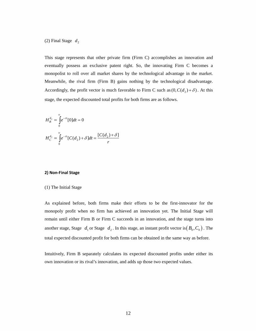
(2) Final Stage 2d
This stage represents that other private firm (Firm C) accomplishes an innovation and
eventually possess an exclusive patent right. So, the innovating Firm C becomes a
monopolist to roll over all market shares by the technological advantage in the market.
Meanwhile, the rival firm (Firm B) gains nothing by the technological disadvantage.
Accordingly, the profit vector is much favorable to Firm C such as 2(0, ( ) )C d δ+ . At this
stage, the expected discounted total profits for both firms are as follows.
2
0
[0] 0d rtBH e dt
∞− == ∫
2 22
0
[ ( ) ][ ( ) ]d rt
CC d
H e C d dtr
δδ
∞− +
+ == ∫
2) Non‐Final Stage
(1) The Initial Stage
As explained before, both firms make their efforts to be the first-innovator for the
monopoly profit when no firm has achieved an innovation yet. The Initial Stage will
remain until either Firm B or Firm C succeeds in an innovation, and the stage turns into
another stage, Stage 1d or Stage 2d . In this stage, an instant profit vector is ( )0 0,B C . The
total expected discounted profit for both firms can be obtained in the same way as before.
Intuitively, Firm B separately calculates its expected discounted profits under either its
own innovation or its rival’s innovation, and adds up those two expected values.

13
( ) ( )00 10 0
( ) ( )rt rtB uH e B b dt e B d dt d
τ
τδ ψ τ τ
∞ ∞− −− + +⎡ ⎤= ⎢ ⎥⎣ ⎦∫ ∫ ∫
+ ( ) ( )00 00 ( )rt rt
ne B b dt e dt dτ
τψ τ τ
∞ ∞− −− +⎡ ⎤⎢ ⎥⎣ ⎦∫ ∫ ∫
where [ ]( ) ( )( ) ( ) b cu b e β γ τψ τ β − += and [ ]( ) ( )( ) ( ) c b
n c e γ β τψ τ γ − +=
Firm B’s entire expectation is eventually simplified as follows.
10 0[ ] ( )
( ) ( )[ ]d
BB
B b b HH
r b cβ
β γ− +
=+ +
where 1 1[ ( ) ]dB
B dH
rδ+
=
Firm C also finds its expected discounted profit in a similar way as Firm B.
( ) ( )00 20 0
( ) ( )rt rtC nH e C c dt e C d dt d
τ
τδ ψ τ τ
∞ ∞− −= − + +⎡ ⎤⎢ ⎥⎣ ⎦∫ ∫ ∫
+ ( ) ( )00 00 ( )rt rt
ue C c dt e dt dτ
τψ τ τ
∞ ∞− −− +⎡ ⎤⎢ ⎥⎣ ⎦∫ ∫ ∫
where [ ]( ) ( )( ) ( ) b cu b e β γ τψ τ β − += and [ ]( ) ( )( ) ( ) c b
n c e γ β τψ τ γ − +=
By expectation, Firm C’s profit is simplified as a function, depending on two different
success rates.
20 0[ ] ( )
( ) ( )[ ]d
CC
C c c HH
r b cγ
β γ− +
+ += where 2 2[ ( ) ]d
CC d
Hr
δ+=
As similar as the previous case, a Nash equilibrium will be found in this Initial stage
because one firm maximizes its expected discounted profit function while the other firm
maximizes in the same manner.

14
From the first order condition0
0BHb
∂=
∂, a best response function is derived such as
( )Rb b c= . Similarly, a best response function ( )Rc c b= is derived from the first order
condition0
0CHc
∂=
∂.
From two conditions above, a Nash equilibrium is derived as ( , )N Nb c . The derived Nash
equilibrium supports the completion of backward induction since the entire innovation
game was reduced to the Initial Stage. As explained before, the innovation race is a huge
sequential game under an infinite horizon, and an innovation randomly occurs. That is, no
one knows when an innovation may realize, and, as soon as either firm succeeds in
innovating, the stage changes into a final stage in which firms stop spending for R&D. The
fact that an arrival of a final stage depends on the randomly distributed variableτ requires
the new form of discount factor[ ]1 ( ) ( )r b cβ γ+ + + , constituting of two success rates.
The equilibrium expected total discounted profits for both firms are as follows.
Firm B’s expected total discounted profit in the Initial Stage is
10
0
( )( )
( ) ( )
N N
B N N
B dB b b
rHr b c
δβ
β γ
+− +
=+ +
⎡ ⎤⎡ ⎤⎣ ⎦ ⎢ ⎥⎣ ⎦
Firm C’s expected total discounted profit in the Initial Stage is
20
0
( )( )
( ) ( )
N N
C N N
C dC c c
rHr b c
δγ
β γ
+− +
=+ +
⎡ ⎤⎡ ⎤⎣ ⎦ ⎢ ⎥⎣ ⎦
Uncertainty of the government-sponsored projects
As discussed, the government’s project can be completed either before or after a firm
innovates. A completion of the government’s project before a private innovation mainly

15
enhances duopoly profits. It also affects both firms’ potential discounted monopoly profits
in the final stage. Meanwhile, a completion after a private innovation provides the firms
the specially enhanced monopoly profits. However, a private firm does not know when a
completion might happen. Let 1π denote the probability of a completion before a private
innovation, and similarly, 2π denotes the probability of a completion after a private
innovation. Both firms can average the derived expected profits over two states and find
the overall expected profits.
Sometimes, a completion of the government project is not guaranteed because of budget
problems even though the government makes all efforts. So, private firms face two
situations. First, the government makes sure that the project will be complete either before
or after a private innovation. Second, the government does not make sure a completion of
the project despite its all efforts. The implication is that the government may not be
responsible for uncertain circumstances such as unexpected costs behind the project.
Usually, financing a public project is limited due to the constrained budget. In the case that
the government has the difficulty to raise additional funds, the government’ project might
make no progress and remain incomplete.
1) Certainty case ( 1 2 1π π+ = )
In this case, the government’s project must be completed either before or after a private
innovation. That is, the government makes firms sure that a supportive innovation will
happen despite some restrictive situations such as budget problems. A completion of the
project may require much expenditure however the government guarantees a private sector
a completion of the project. Thus, private firms can calculate their overall expected profits.
Both firms’ overall expected profits are following.
Firm B’s overall expected total discounted profit is
16
[ ]( )
[ ]1 10 0
01 1
( ) ( )( ) ( )
1( ) ( ) ( ) ( )B
B d B dB b b B b b
r rHr b c r b c
δβ β
π πβ γ β γ
+ Ω ++Ω − + − +
′ = + −+ + + +
⎡ ⎤ ⎡ ⎤⎡ ⎤ ⎡ ⎤⎢ ⎥ ⎢ ⎥⎢ ⎥ ⎢ ⎥⎣ ⎦ ⎣ ⎦⎢ ⎥ ⎢ ⎥⎢ ⎥ ⎢ ⎥⎢ ⎥ ⎢ ⎥⎣ ⎦ ⎣ ⎦
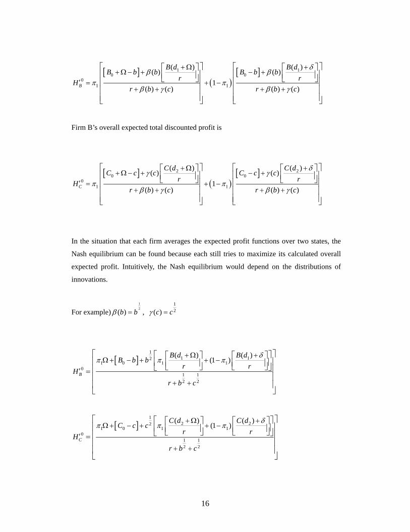
Firm B’s overall expected total discounted profit is
[ ]( )
[ ]2 20 0
01 1
( ) ( )( ) ( )
1( ) ( ) ( ) ( )C
C d C dC c c C c c
r rHr b c r b c
δγ γ
π πβ γ β γ
+Ω ++Ω − + − +
′ = + −+ + + +
⎡ ⎤ ⎡ ⎤⎡ ⎤ ⎡ ⎤⎢ ⎥ ⎢ ⎥⎢ ⎥ ⎢ ⎥⎣ ⎦ ⎣ ⎦⎢ ⎥ ⎢ ⎥⎢ ⎥ ⎢ ⎥⎢ ⎥ ⎢ ⎥⎣ ⎦ ⎣ ⎦
In the situation that each firm averages the expected profit functions over two states, the
Nash equilibrium can be found because each still tries to maximize its calculated overall
expected profit. Intuitively, the Nash equilibrium would depend on the distributions of
innovations.
For example)12
( )b bβ = , 12( )c cγ =
[ ]1
1 121 0 1 1
01 12 2
( ) ( )(1 )
B
B d B dB b b
r rH
r b c
δπ π π
+Ω +Ω + − + + −
′
+ +
⎡ ⎤⎡ ⎤⎡ ⎤ ⎡ ⎤⎢ ⎥⎢ ⎥⎢ ⎥ ⎢ ⎥⎣ ⎦ ⎣ ⎦⎣ ⎦⎢ ⎥=⎢ ⎥⎢ ⎥⎣ ⎦
[ ]1
2 221 0 1 1
01 12 2
( ) ( )(1 )
C
C d C dC c c
r rH
r b c
δπ π π
+Ω +Ω + − + + −
′
+ +
⎡ ⎤⎡ ⎤⎡ ⎤ ⎡ ⎤⎢ ⎥⎢ ⎥⎢ ⎥ ⎢ ⎥⎣ ⎦ ⎣ ⎦⎣ ⎦⎢ ⎥=⎢ ⎥⎢ ⎥⎣ ⎦
17
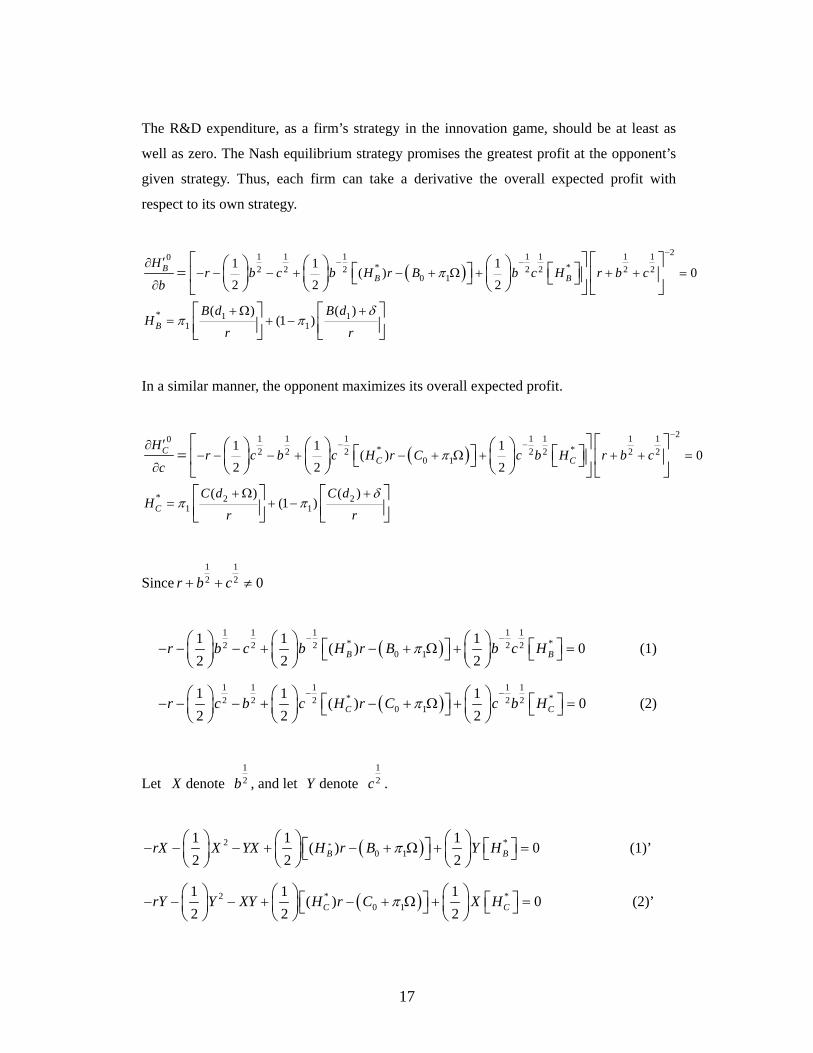
The R&D expenditure, as a firm’s strategy in the innovation game, should be at least as
well as zero. The Nash equilibrium strategy promises the greatest profit at the opponent’s
given strategy. Thus, each firm can take a derivative the overall expected profit with
respect to its own strategy.
( )21 1 1 1 1 1 10
* *2 2 2 2 2 2 20 1
1 1 1( ) 0
2 2 2B
B BH
r b c b H r B b c H r b cb
π
−− −′∂
− − − + − + Ω + + + =∂
⎡ ⎤ ⎡ ⎤⎛ ⎞ ⎛ ⎞ ⎛ ⎞ ⎡ ⎤⎡ ⎤= ⎜ ⎟ ⎜ ⎟ ⎜ ⎟⎢ ⎥ ⎢ ⎥⎣ ⎦ ⎣ ⎦⎝ ⎠ ⎝ ⎠ ⎝ ⎠⎣ ⎦ ⎣ ⎦* 1 1
1 1( ) ( )
(1 )BB d B d
Hr r
δπ π
+ Ω += + −
⎡ ⎤ ⎡ ⎤⎢ ⎥ ⎢ ⎥⎣ ⎦ ⎣ ⎦
In a similar manner, the opponent maximizes its overall expected profit.
( )21 1 1 1 1 1 10
* *2 2 2 2 2 2 20 1
1 1 1( ) 0
2 2 2C
C CH
r c b c H r C c b H r b cc
π
−− −′∂
− − − + − + Ω + + + =∂
⎡ ⎤ ⎡ ⎤⎛ ⎞ ⎛ ⎞ ⎛ ⎞⎡ ⎤ ⎡ ⎤= ⎜ ⎟ ⎜ ⎟ ⎜ ⎟⎢ ⎥ ⎢ ⎥⎣ ⎦ ⎣ ⎦⎝ ⎠ ⎝ ⎠ ⎝ ⎠⎣ ⎦ ⎣ ⎦* 2 2
1 1( ) ( )
(1 )CC d C d
Hr r
δπ π
+ Ω += + −
⎡ ⎤ ⎡ ⎤⎢ ⎥ ⎢ ⎥⎣ ⎦ ⎣ ⎦
Since1 12 2 0r b c+ + ≠
( )1 1 1 1 1
* *2 2 2 2 20 1
1 1 1( ) 0
2 2 2B Br b c b H r B b c Hπ− −
− − − + − + Ω + =⎛ ⎞ ⎛ ⎞ ⎛ ⎞ ⎡ ⎤⎡ ⎤⎜ ⎟ ⎜ ⎟ ⎜ ⎟⎣ ⎦ ⎣ ⎦⎝ ⎠ ⎝ ⎠ ⎝ ⎠ (1)
( )1 1 1 1 1
* *2 2 2 2 20 1
1 1 1( ) 0
2 2 2C Cr c b c H r C c b Hπ− −
− − − + − + Ω + =⎛ ⎞ ⎛ ⎞ ⎛ ⎞ ⎡ ⎤⎡ ⎤⎜ ⎟ ⎜ ⎟ ⎜ ⎟⎣ ⎦ ⎣ ⎦⎝ ⎠ ⎝ ⎠ ⎝ ⎠ (2)
Let X denote 12b , and let Y denote
12c .
( )*2 *0 1
1 1 1( ) 0
2 2 2B BrX X YX H r B Y Hπ− − − + − + Ω + =⎛ ⎞ ⎛ ⎞ ⎛ ⎞⎡ ⎤ ⎡ ⎤⎜ ⎟ ⎜ ⎟ ⎜ ⎟ ⎣ ⎦⎣ ⎦⎝ ⎠ ⎝ ⎠ ⎝ ⎠ (1)’
( )2 * *0 1
1 1 1( ) 0
2 2 2C CrY Y XY H r C X Hπ− − − + − + Ω + =⎛ ⎞ ⎛ ⎞ ⎛ ⎞⎡ ⎤ ⎡ ⎤⎜ ⎟ ⎜ ⎟ ⎜ ⎟⎣ ⎦ ⎣ ⎦⎝ ⎠ ⎝ ⎠ ⎝ ⎠ (2)’

18
Since the firms, as the incumbent duopolists, have equal market shares under the same
circumstances in the industry, the market profits should be equally distributed to both firms.
Furthermore, the potential monopoly profit in a final stage would be the same for both
firms because they target the same type of technological improvement through R&D
project. Then, the symmetry condition can be derived from (1)’ and (2)’ because the
duopoly profits and the potential monopoly profits are identical for both firms. The
symmetric condition actually implies that one firm chooses its R&D expenditure based on
the expectation that its opponent would make the same choice under all the same
circumstances.
Under a symmetry condition ( X Y= ), Firm B chooses its Nash Equilibrium R&D
expenditure from the following equation.
( )2 * *0 13 2 ( ) ( ) 0B BX r H X H r B π+ − − − + Ω =⎡ ⎤ ⎡ ⎤⎣ ⎦ ⎣ ⎦ where 0 0B C= , * *
B CH H=
The equation above implies that Firm B still needs to find the profit-maximizing R&D
choice from the clue that Firm C would actually choose the same as Firm B. In the
opposite way, Firm C obtains the profit-maximizing R&D choice by the same speculation.
The symmetric condition simply tells that both firms provide a clue for each other and they
equally reach the Nash Equilibrium.
2* * *0 1( ) 2 2 ( ) 12 ( ) ( )
6B B BH r r H H r B
X Yπ− ± − + − + Ω
′ ′= =⎡ ⎤ ⎡ ⎤ ⎡ ⎤⎣ ⎦ ⎣ ⎦ ⎣ ⎦
, 0X Y′ ′ >
If *( ) 2 0BH r− ≥
2* * *0 1( ) 2 2 ( ) 12 ( ) ( )
6B B BH r r H H r B
X Yπ− − + − + Ω
′ ′= =⎡ ⎤ ⎡ ⎤ ⎡ ⎤+⎣ ⎦ ⎣ ⎦ ⎣ ⎦

19
( )2
2* * *0 1( ) 2 2 ( ) 12 ( )
6B B BH r r H H r B
b cπ− + − + − + Ω
′ ′= =
⎡ ⎤⎡ ⎤ ⎡ ⎤ ⎡ ⎤⎣ ⎦ ⎣ ⎦ ⎣ ⎦⎢ ⎥⎢ ⎥⎢ ⎥⎣ ⎦
( ),b c′ ′ is the Nash Equilibrium. As both firms expect, they actually obtain the same
equilibrium R&D choices.
The government tries to figure out whether the public projects have an effect on the
innovative activities of private firms. First of all, the government aims in inspiring
innovative activities. The government still has a question if any increased probability of a
completion of the project before a private innovation has an impact on innovative activities.
To see what effects the increased probability ( 1π ) would bring in the industry, a
comparative study is suggested for 1π and the Nash Equilibrium R&D expenditures.
Depending on the size of 1π , the Nash Equilibrium R&D expenditures of both firms
would change. If we actually take a derivative X ′ with respect to 1π then the following
result is obtained.
1* * *2 2* * *
0 11 1 1 1
1 1 2 ( ) 4 ( ) ( ) ( 2) 2 ( ) 4 46 2
B B BB B B
dH dH dHdX r H H r B r H rd d d d
ππ π π π
−⎡ ⎤⎡ ⎤′ ⎡ ⎤⎡ ⎤ ⎡ ⎤ ⎡ ⎤= + − + − + Ω − − + − Ω⎢ ⎥⎢ ⎥⎣ ⎦ ⎣ ⎦ ⎣ ⎦⎢ ⎥⎣ ⎦⎢ ⎥⎣ ⎦⎣ ⎦
where 1 1
1
* ( ) ( )0BdH B d B d
d r r
δ
π
+ Ω += − <⎡ ⎤ ⎡ ⎤⎢ ⎥ ⎢ ⎥⎣ ⎦ ⎣ ⎦
∴1
0dX
dπ
′< ⇒
1
0db
dπ
′<
The inequality above tells that a raised probability for a completion of the project actually
reduces the R&D expenditures for both firms. The implication is that as the government
tries harder to complete the project before a private innovation both private firms are not
so motivated for their innovative activities because a completed government-project

20
mainly enhances both firms’ duopoly profits. More intuitively, the increased probability
( 1π ) reduces the averages ( *BH and *
CH ) of discounted monopoly profits. The direct
reason is that an increase in 1π necessarily implies a decrease in 2π under certainty. It
means that an increased chance in one state reduces the chance of the other state.
Unfortunately, both firms can expect higher monopoly profits at 2π than at 1π . Thus,
private firms’ average of (discounted) monopoly profit would be decreased as 1π
increases. That is,
1 1
1
* ( ) ( )0BdH B d B d
d r r
δ
π
+ Ω += − <⎡ ⎤ ⎡ ⎤⎢ ⎥ ⎢ ⎥⎣ ⎦ ⎣ ⎦
where * 1 11 1
( ) ( )(1 )B
B d B dH
r r
δπ π
+ Ω += + −
⎡ ⎤ ⎡ ⎤⎢ ⎥ ⎢ ⎥⎣ ⎦ ⎣ ⎦
0)()( 22
1
*
<⎥⎦⎤
⎢⎣⎡ +
−⎥⎦⎤
⎢⎣⎡ Ω+
=r
dCr
dCddHC δπ
where * 2 21 1
( ) ( )(1 )C
C d C dH
r r
δπ π
+ Ω += + −
⎡ ⎤ ⎡ ⎤⎢ ⎥ ⎢ ⎥⎣ ⎦ ⎣ ⎦
Meanwhile, both firms’ averages ( Ω+− 10 πbB and Ω+− 10 πcC ) of duopoly profits
definitely increase as 1π increases. So the firms are less motivated for their own
innovation.
2) Uncertainty case ( 1 2 1π π+ < , where 10 1π≤ < and 20 1π≤ < )
This case represents that the government-project might not be completed for private firms
due to some reasons, different from the certainty case. In a private sector, firms would
calculate their overall expected profits under uncertainty by averaging both states as
follows. Both firms’ overall expected profits are following.
21
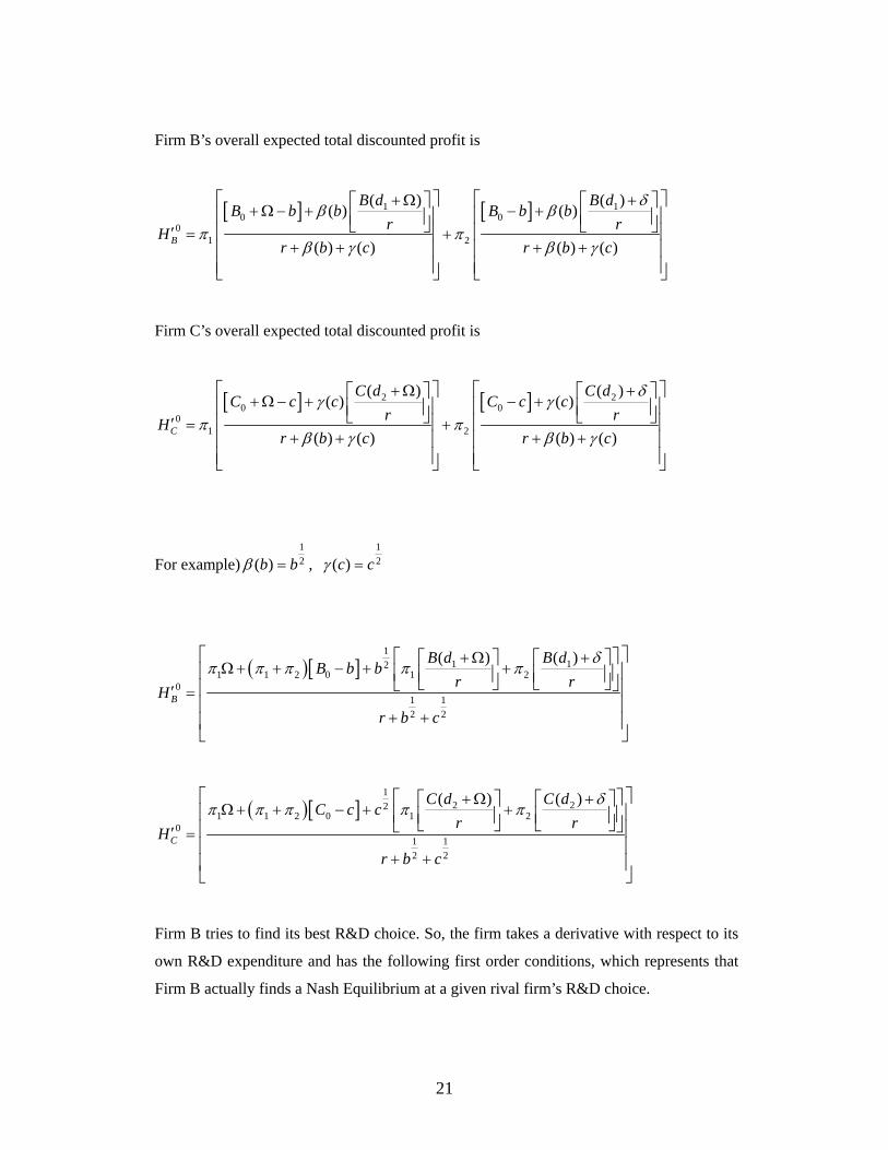
Firm B’s overall expected total discounted profit is
[ ] [ ]1 10 0
01 2
( ) ( )( ) ( )
( ) ( ) ( ) ( )B
B d B dB b b B b b
r rHr b c r b c
δβ β
π πβ γ β γ
+ Ω ++Ω − + − +
′ = ++ + + +
⎡ ⎤ ⎡ ⎤⎡ ⎤ ⎡ ⎤⎢ ⎥ ⎢ ⎥⎢ ⎥ ⎢ ⎥⎣ ⎦ ⎣ ⎦⎢ ⎥ ⎢ ⎥⎢ ⎥ ⎢ ⎥⎢ ⎥ ⎢ ⎥⎣ ⎦ ⎣ ⎦
Firm C’s overall expected total discounted profit is
[ ] [ ]2 20 0
01 2
( ) ( )( ) ( )
( ) ( ) ( ) ( )C
C d C dC c c C c c
r rHr b c r b c
δγ γ
π πβ γ β γ
+Ω ++Ω − + − +
′ = ++ + + +
⎡ ⎤ ⎡ ⎤⎡ ⎤ ⎡ ⎤⎢ ⎥ ⎢ ⎥⎢ ⎥ ⎢ ⎥⎣ ⎦ ⎣ ⎦⎢ ⎥ ⎢ ⎥⎢ ⎥ ⎢ ⎥⎢ ⎥ ⎢ ⎥⎣ ⎦ ⎣ ⎦
For example)12( )b bβ = ,
12( )c cγ =
( )[ ]1
1 121 1 2 0 1 2
01 12 2
( ) ( )
B
B d B dB b b
r rH
r b c
δπ π π π π
+Ω +Ω+ + − + +
′ =
+ +
⎡ ⎤⎡ ⎤⎡ ⎤ ⎡ ⎤⎢ ⎥⎢ ⎥⎢ ⎥ ⎢ ⎥⎣ ⎦ ⎣ ⎦⎣ ⎦⎢ ⎥⎢ ⎥⎢ ⎥⎣ ⎦
( )[ ]1
2 221 1 2 0 1 2
01 12 2
( ) ( )
C
C d C dC c c
r rH
r b c
δπ π π π π
+Ω +Ω+ + − + +
′ =
+ +
⎡ ⎤⎡ ⎤⎡ ⎤ ⎡ ⎤⎢ ⎥⎢ ⎥⎢ ⎥ ⎢ ⎥⎣ ⎦ ⎣ ⎦⎣ ⎦⎢ ⎥⎢ ⎥⎢ ⎥⎣ ⎦
Firm B tries to find its best R&D choice. So, the firm takes a derivative with respect to its
own R&D expenditure and has the following first order conditions, which represents that
Firm B actually finds a Nash Equilibrium at a given rival firm’s R&D choice.

22
[ ] [ ]( )1 1 1 1 1
* *2 2 2 2 21 2 1 2 0 10
21 12 2
1 1 1
2 2 21 ( )
0B B
B
r b c b H r B b c HH
br b c
π π π π π− −
− + + − − + − + + Ω +′∂
= =∂
+ +
⎡ ⎤⎛ ⎞ ⎛ ⎞ ⎛ ⎞⎡ ⎤ ⎡ ⎤⎜ ⎟ ⎜ ⎟⎜ ⎟⎢ ⎥⎣ ⎦ ⎣ ⎦⎝ ⎠ ⎝ ⎠⎝ ⎠⎣ ⎦⎡ ⎤⎢ ⎥⎣ ⎦
* 1 11 2
( ) ( )B
B d B dH
r r
δπ π
+ Ω += +
⎡ ⎤ ⎡ ⎤⎢ ⎥ ⎢ ⎥⎣ ⎦ ⎣ ⎦
In a similar manner, the opponent maximizes its overall expected profit by the first order
condition.
[ ] [ ]( )1 1 1 1 1
* *2 2 2 2 21 2 1 2 0 10
21 12 2
1 1 1
2 2 21 ( )
0C C
C
r c b c H r C c b HH
cr b c
π π π π π− −
− + + − − + − + + Ω +′∂
= =∂
+ +
⎡ ⎤⎛ ⎞ ⎛ ⎞ ⎛ ⎞⎡ ⎤ ⎡ ⎤⎜ ⎟ ⎜ ⎟⎜ ⎟⎢ ⎥⎣ ⎦⎣ ⎦⎝ ⎠ ⎝ ⎠⎝ ⎠⎣ ⎦⎡ ⎤⎢ ⎥⎣ ⎦
* 2 21 2
( ) ( )C
C d C dH
r r
δπ π
+ Ω += +
⎡ ⎤ ⎡ ⎤⎢ ⎥ ⎢ ⎥⎣ ⎦ ⎣ ⎦
From the two first order conditions, the new necessary conditions for both firms’ overall
expected profits are found as follows since1 12 2 0r b c+ + ≠ .
[ ] [ ]( )1 1 1 1 1
* *2 2 2 2 21 2 1 2 0 1
1 1 1
2 2 21 ( ) 0B Br b c b H r B b c Hπ π π π π
− −− + + − − + − + + Ω + =
⎛ ⎞ ⎛ ⎞ ⎛ ⎞⎡ ⎤ ⎡ ⎤⎜ ⎟ ⎜ ⎟⎜ ⎟ ⎣ ⎦ ⎣ ⎦⎝ ⎠ ⎝ ⎠⎝ ⎠
(1)
[ ] [ ]( )1 1 1 1 1
1 1* *2 2 2 2 21 2 1 2 0 1
2 2
1
21 ( ) 0C Cr c b c H r C c b Hπ π π π π
− −− + + − − + − + + Ω + =
⎛ ⎞ ⎛ ⎞ ⎛ ⎞⎡ ⎤ ⎡ ⎤⎜ ⎟ ⎜ ⎟⎜ ⎟ ⎣ ⎦ ⎣ ⎦⎝ ⎠ ⎝ ⎠⎝ ⎠
(2)

23
Let X denote 12b , and let Y denote
12c for simplicity.
[ ] [ ]( )2 * *1 2 1 2 0 1
1 1 1
2 2 21 ( ) 0B BrX X YX H r B Y Hπ π π π π− + + − − + − + + Ω + =
⎛ ⎞ ⎛ ⎞ ⎛ ⎞⎡ ⎤ ⎡ ⎤⎜ ⎟ ⎜ ⎟⎜ ⎟ ⎣ ⎦ ⎣ ⎦⎝ ⎠ ⎝ ⎠⎝ ⎠
(1)’
[ ] [ ]( )2 * *1 2 1 2 0 1
1 1 1
2 2 21 ( ) 0C CrY Y XY H r C X Hπ π π π π− + + − − + − + + Ω + =
⎛ ⎞ ⎛ ⎞ ⎛ ⎞⎡ ⎤ ⎡ ⎤⎜ ⎟ ⎜ ⎟⎜ ⎟ ⎣ ⎦ ⎣ ⎦⎝ ⎠ ⎝ ⎠⎝ ⎠
(2)’
As similar as the certainty case, both firms would choose their R&D expenditures by
expectation that the rival would determine its choice based on the same expectation since
both firms make their decisions under identical circumstances. They would reach a
symmetric equilibrium R&D choice. Under a symmetry condition, Firm B has the new
condition for maximizing its overall expected profit as follows. The simplified form
implies that Firm B narrows its choices by a clue that its rival Firm C would choose the
same as itself.
[ ] [ ]( )2 * *1 2 1 2 0 14 2 ( ) ( ) 0B BX r H X H r Bπ π π π π− + + − − − + + Ω =⎡ ⎤ ⎡ ⎤⎡ ⎤⎣ ⎦ ⎣ ⎦ ⎣ ⎦
[ ] [ ][ ]( )
2* * *1 2 1 2 0 1
1 2
( ) 2 2 ( ) 4 4 ( ) ( )
2 4B B BH r r H H r B
X Yπ π π π π
π π
− ± − + − + − + + Ω′ ′= =
− +
⎡ ⎤ ⎡ ⎤ ⎡ ⎤⎡ ⎤⎣ ⎦⎣ ⎦ ⎣ ⎦ ⎣ ⎦
, 0X Y′ ′ >
If *( ) 2 0H rB − ≥
[ ] [ ][ ]( )
2* * *1 2 1 2 0 1
1 2
( ) 2 2 ( ) 4 4 ( ) ( )
2 4B B BH r r H H r B
X Yπ π π π π
π π
+− − + − + − + + Ω′ ′= =
− +
⎡ ⎤ ⎡ ⎤ ⎡ ⎤⎡ ⎤⎣ ⎦⎣ ⎦ ⎣ ⎦ ⎣ ⎦

24
Both Firm B and Firm C actually choose the same R&D expenditure by the same
expectation toward its rival’s strategic behavior. The expectation actually leads to the
symmetric result.
[ ] [ ][ ]( )
22* * *
1 2 1 2 0 1
1 2
( ) 2 2 ( ) 4 4 ( ) ( )
2 4
B B BH r r H H r Bb c
π π π π π
π π
− + − + − + − + + Ω′ ′= =
− +
⎡ ⎤⎡ ⎤ ⎡ ⎤ ⎡ ⎤⎡ ⎤⎣ ⎦⎣ ⎦ ⎣ ⎦ ⎣ ⎦⎢ ⎥⎢ ⎥⎢ ⎥⎣ ⎦
( ),b c′ ′ is the Nash Equilibrium.
If the government enlarges the budget for the public project and increases the probability
of a completion, how do private firms respond to this favorable government’s support? Do
they increase or decrease their innovative activities?
[ ] ( )( ) [ ] ( )( )* 1 1( 1) ( 2)*2 2
1 2 1 21 1 1
1 12 4 2 ( 1) 2 4 ( 1)
6 2B
BdHdX d
H r Md d d
π π π ππ π π
− −−′ Μ= + Μ − + + − + − − + −
⎡ ⎤⎡ ⎤ ⎡ ⎤⎡ ⎤⎡ ⎤ ⎡ ⎤⎢ ⎥⎢ ⎥ ⎣ ⎦ ⎣ ⎦⎣ ⎦⎢ ⎥⎣ ⎦⎣ ⎦⎣ ⎦
where [ ] [ ]2* *
1 2 1 2 0 12 ( ) 4 4 ( ) ( )B BM r H H r Bπ π π π π= − + − + − + + Ω⎡ ⎤ ⎡ ⎤⎡ ⎤⎣ ⎦⎣ ⎦ ⎣ ⎦
and
[ ]* *
* *1 2 1 2 0 1 0 2 0
1 1 1
2 ( ) 2 16 4( ) 16 8 4 16 8 8B BB B
dH dHdMH r r H r B B B
d d dπ π π π π π
π π π= − + − + − − Ω + Ω + Ω − + +⎡ ⎤ ⎡ ⎤⎣ ⎦⎣ ⎦
Different from the certainty case, 1
dX
dπ
′is not necessarily less than zero. It is actually
ambiguous. 1
dX
dπ
′ could be greater than zero for some cases. For example, if
1
dM
dπ is
greater than or equal to zero then the private firms’ R&D choices would increase in 1π .
Implicatively, the private firms may spend more expenditure for R&D, under uncertainty,
although a completion of the government project mainly enhances the firms’ duopoly
profits.

25
01
dM
dπ≥
implies
[ ]* *
* *1 2 1 2 0 1 0 2 0
1 1
2 ( ) 2 16 4( ) 16 8 4 16 8 8 0B BB B
dH dHH r r H r B B B
d dπ π π π π π
π π− + − + − − Ω + Ω + Ω − + + ≥⎡ ⎤ ⎡ ⎤⎣ ⎦⎣ ⎦
where *
1
1
( )BdH B d
d rπ
+ Ω=⎡ ⎤⎢ ⎥⎣ ⎦
and * 1 11 2
( ) ( )B
B d B dH
r r
δπ π
+ Ω += +
⎡ ⎤ ⎡ ⎤⎢ ⎥ ⎢ ⎥⎣ ⎦ ⎣ ⎦
Rearrange all the terms by 1π and 2π .
( )( ) [ ] [ ]1 111 1 2 1 12 2
2 ( ) ( )2 ( )( ) 5 4 ( ) ( )
B d B dB dB d B d B d
r r
δπ π δ
+ + Ω+ Ω+ Ω − + − + − + Ω
⎡ ⎤⎡ ⎤⎡ ⎤⎢ ⎥⎢ ⎥⎢ ⎥⎣ ⎦⎣ ⎦ ⎣ ⎦
[ ]1 012 ( ) 16 16 0B d B+ + Ω − Ω − ≥
The following conditions actually satisfy the inequality above since 1 0π ≥ and 2 0π ≥ .
(1) 21 5 / 2( ) rB d ⎡ ⎤
⎢ ⎥⎣ ⎦+ Ω ≥
(2) ( )( ) [ ] [ ]21 1 1 1/ 2( ) ( ) 4 ( ) ( )rB d B d B d B dδ δ⎡ ⎤
⎢ ⎥⎣ ⎦+ + Ω ≥ + + + Ω⎡ ⎤⎣ ⎦
(3) ( ) ( )1 04 / 3( )B d B+ Ω ≥ + Ω
Actually, the conditions above can be simplified. First, if ( ) ( )205 / 2 4 / 3r B⎡ ⎤
⎢ ⎥⎣ ⎦ ≥ + Ω then the
intersection between (1) and (3) should be 25 / 2( )1 rB d ⎡ ⎤⎢ ⎥⎣ ⎦+ Ω ≥ . In this case, we can
conclude that ( ) ( )08/15r B≤ − + Ω or ( ) ( )08/15r B≥ + Ω . In fact, ( ) ( )08/15r B≥ + Ω
since 0 1r< < . ( )0B + Ω should be less than ( )15/8 .
Second, if ( ) ( )205 / 2 4 /3r B⎡ ⎤ ≤⎢ ⎥⎣ ⎦ + Ω then the intersection between (1) and (3) will be
( ) ( )1 04 / 3( )B d B+ Ω ≥ + Ω . So, ( ) ( ) ( ) ( )0 08/15 8/15B r B− + Ω ≤ ≤ + Ω . r actually takes

26
some value between 0 and ( ) ( )08/15 B + Ω since 0 1r≤ < .
If ( )0B + Ω is at least as great as ( )15/8 then the imposed constraint
( ) ( )205 / 2 4 /3r B⎡ ⎤
⎢ ⎥⎣ ⎦ ≥ + Ω is meaningless in this argument and the three conditions above
should be reduced to the following two conditions,
( )( ) [ ] [ ]21 1 1 1/ 2( ) ( ) 4 ( ) ( )rB d B d B d B dδ δ⎡ ⎤
⎢ ⎥⎣ ⎦+ + Ω ≥ + + + Ω⎡ ⎤⎣ ⎦
and ( ) ( )1 04 / 3( )B d B+ Ω ≥ + Ω .
So far, we have discussed under what cases the private firms may increase their R&D
expenditures though their enhanced duopoly profits by a completion of the government-
project.
Under certainty case, an increased funding for completing the project reduces R&D
expenditures of the private firms. In fact, an increased probability ( 1π ) of completion of
the project improves the firms’ averages of duopoly profits but reduces averages of
(discounted) monopoly profits for both firms. It results from the fact that an increased
probability of one state necessarily means a reduction of probability of the other state
under certainty case. Due to the reduced averages of monopoly profits and the improved
averages of duopoly profits, the firms would lower their levels of R&D expenditures.
However, both the averages of duopoly profits and the averages of monopoly profits
improve under uncertainty case when 1π increases. Unlike the certainty case, the
averages of monopoly profits increase in 1π as below.
0)( 1
1
*
>⎥⎦⎤
⎢⎣⎡ Ω+
=r
dCddHB
π where * 1 1
1 2( ) ( )
BB d B d
Hr r
δπ π
+ Ω += +
⎡ ⎤ ⎡ ⎤⎢ ⎥ ⎢ ⎥⎣ ⎦ ⎣ ⎦
0)( 2
1
*
>⎥⎦⎤
⎢⎣⎡ Ω+
=r
dCddHC
π where * 2 2
1 2( ) ( )
CC d C d
Hr r
δπ π
+ Ω += +
⎡ ⎤ ⎡ ⎤⎢ ⎥ ⎢ ⎥⎣ ⎦ ⎣ ⎦
The averages of monopoly profits would make the firms confused about their R&D

27
decisions. That is, the firms would be willing to reduce their R&D spending by the
improved averages of duopoly profits and be ready to increase the R&D spending for the
improved averages of monopoly profits. In this case, the firms may increase or decrease
their R&D expenditures, depending on the situation. If an increase in 1π more strongly
impacts the averages of duopoly profits then the private firms would be less motivated for
an innovation so their R&D expenditures would be decreased. On the contrary, if the
increased 1π more strongly impacts the averages of monopoly profits then they would be
more motivated to innovate earlier. Thus, their R&D expenditures would be increased.
Intuitively, the uncertainty makes both firms to remind that they are involved in an
innovation race for their future. Thus, if the government increases the fund to complete the
project and enhances the duopoly profits under uncertainty then both firms might increase
their R&D expenditures, in some cases, for their monopoly profits in the future.
Implicatively, they are forced to spend more for their innovative activities under
uncertainty because the uncertainty reminds them their competition for an innovation.
3. Drastic Innovation
Unlike the previous case that both firms equally share the market, this innovation race
starts by a monopoly and ends up with a monopoly. In detail, the incumbent firm has a
monopoly profit before the entrant firm succeeds in an innovation. The entrant’s
innovation would actually replace a monopolist. However, the entrant would gain nothing
until it successfully innovates through its continuous R&D expenditure. Up to the timing
of any innovation, the incumbent firm still obtains its monopoly profit. With its own
innovation, the incumbent firm improves its monopoly profit. With the entrant’s innovation,
the incumbent firm will be replaced for good by the entrant firm. For example, a medicine
represents the drastic innovation well. Usually, a newly-invented medicine monopolizes all
market shares and is replaced by the new medicine that has smaller side effect. In this way,
a medicine evolves to the smallest side effect (Obesity, Anti-depression, and so on). The
pharmacy industry is closely related with the government project because of a lot of R&D
costs.

28
Here, Firm B is the incumbent firm and Firm C is the entrant firm. Both firms’ overall
expected profits are following.
Firm B’s overall expected total discounted profit is
[ ] [ ]1 10 0
01 2
( ) ( )( ) ( )
( ) ( ) ( ) ( )B
B d B dB b b B b b
r rHr b c r b c
δβ β
π πβ γ β γ
+ Ω ++Ω − + − +
′ = ++ + + +
⎡ ⎤ ⎡ ⎤⎡ ⎤ ⎡ ⎤⎢ ⎥ ⎢ ⎥⎢ ⎥ ⎢ ⎥⎣ ⎦ ⎣ ⎦⎢ ⎥ ⎢ ⎥⎢ ⎥ ⎢ ⎥⎢ ⎥ ⎢ ⎥⎣ ⎦ ⎣ ⎦
Firm B’s overall expected total discounted profit is
[ ] [ ]2 2
01 2
( ) ( )0 ( ) 0 ( )
( ) ( ) ( ) ( )C
C d C dc c c c
r rHr b c r b c
δγ γ
π πβ γ β γ
+Ω +− + − +
′ = ++ + + +
⎡ ⎤ ⎡ ⎤⎡ ⎤ ⎡ ⎤⎢ ⎥ ⎢ ⎥⎢ ⎥ ⎢ ⎥⎣ ⎦ ⎣ ⎦⎢ ⎥ ⎢ ⎥⎢ ⎥ ⎢ ⎥⎢ ⎥ ⎢ ⎥⎣ ⎦ ⎣ ⎦
For example)12( )b bβ = ,
12( )c cγ =
( )[ ]1
1 121 1 2 0 1 2
01 12 2
( ) ( )
B
B d B dB b b
r rH
r b c
δπ π π π π
+Ω +Ω+ + − + +
′ =
+ +
⎡ ⎤⎡ ⎤⎡ ⎤ ⎡ ⎤⎢ ⎥⎢ ⎥⎢ ⎥ ⎢ ⎥⎣ ⎦ ⎣ ⎦⎣ ⎦⎢ ⎥⎢ ⎥⎢ ⎥⎣ ⎦
( )[ ]1
2 221 2 1 2
01 12 2
( ) ( )0
C
C d C dc c
r rH
r b c
δπ π π π
+Ω ++ − + +
′ =
+ +
⎡ ⎤⎡ ⎤⎡ ⎤ ⎡ ⎤⎢ ⎥⎢ ⎥⎢ ⎥ ⎢ ⎥⎣ ⎦ ⎣ ⎦⎣ ⎦⎢ ⎥⎢ ⎥⎢ ⎥⎣ ⎦

29
From the first order conditions,
[ ] [ ]( )1 1 1 1 1
* *2 2 2 2 21 2 1 2 0 1
1 1 11 ( ) 0
2 2 2B Br b c b H r B b c Hπ π π π π− −
− + + − − + − + + Ω + =⎛ ⎞ ⎛ ⎞ ⎛ ⎞⎡ ⎤ ⎡ ⎤⎜ ⎟ ⎜ ⎟ ⎜ ⎟ ⎣ ⎦⎣ ⎦⎝ ⎠ ⎝ ⎠ ⎝ ⎠ (1)
[ ]1 1 1 1 1
* *2 2 2 2 21 2
1 1 11 ( ) 0
2 2 2C Cr c b c H r c b Hπ π− −
− + + − − + + =⎛ ⎞ ⎛ ⎞ ⎛ ⎞⎡ ⎤ ⎡ ⎤⎜ ⎟ ⎜ ⎟ ⎜ ⎟⎣ ⎦ ⎣ ⎦⎝ ⎠ ⎝ ⎠ ⎝ ⎠ (2)
Let X denote 12b , and let Y denote
12c .
[ ] [ ]( )2 * *1 2 1 2 0 1
1 1 11 ( ) 0
2 2 2B BrX X YX H r B Y Hπ π π π π− + + − − + − + + Ω + =⎛ ⎞ ⎛ ⎞ ⎛ ⎞⎡ ⎤ ⎡ ⎤⎜ ⎟ ⎜ ⎟ ⎜ ⎟ ⎣ ⎦⎣ ⎦⎝ ⎠ ⎝ ⎠ ⎝ ⎠
(1)’
[ ] 2 * *1 2
1 1 11 ( ) 0
2 2 2C CrY Y XY H r X Hπ π− + + − − + + =⎛ ⎞ ⎛ ⎞ ⎛ ⎞⎡ ⎤ ⎡ ⎤⎜ ⎟ ⎜ ⎟ ⎜ ⎟⎣ ⎦ ⎣ ⎦⎝ ⎠ ⎝ ⎠ ⎝ ⎠ (2)’
By comparative static analysis, we can recognize how private firms would respond to the
government’s favorable policy such as enlarging the budget for the public project and
increasing the probability of a completion of the public project. By total differentiation,
[ ]2 20 1 0 2 1 2
1 1 1 1 1 12 1
2 2 2 2 2 2 2 2Y r
X B d X B d dXπ π π π− − Ω + − + + − − −⎡ ⎤ ⎡ ⎤ ⎡ ⎤⎢ ⎥ ⎢ ⎥ ⎢ ⎥⎣ ⎦ ⎣ ⎦ ⎣ ⎦
*10
2 BH X dY+ − =⎡ ⎤⎡ ⎤⎣ ⎦⎢ ⎥⎣ ⎦ (3)
[ ]2 2 *1 2 1 2
1 1 1 12 1 0
2 2 2 2 2 2 CX r
Y d Y d dX H Y dXπ π π π+ + + − − − + − =⎡ ⎤ ⎡ ⎤ ⎡ ⎤ ⎡ ⎤⎡ ⎤⎣ ⎦⎢ ⎥ ⎢ ⎥ ⎢ ⎥ ⎢ ⎥⎣ ⎦ ⎣ ⎦ ⎣ ⎦ ⎣ ⎦ (4)

30
By transformation, the equations (3) and (4) can be rewritten as (3)’ and (4)’.
1 2 0Ad Bd CdX EdYπ π+ + + = (3)’
1 2 0A d B d C dX E dYπ π′ ′ ′ ′+ + + = (4)’
where 20
1 1 12 2 2
A X B⎡ ⎤= − − Ω⎢ ⎥⎣ ⎦, 2
01 12 2
B X B⎡ ⎤= −⎢ ⎥⎣ ⎦, [ ]1 2
12 12 2 2
Y rC π π⎡ ⎤= + − − −⎢ ⎥⎣ ⎦
*12 BE H X⎡ ⎤⎡ ⎤= −⎣ ⎦⎢ ⎥⎣ ⎦
, 212
A Y⎡ ⎤′ = ⎢ ⎥⎣ ⎦, 21
2B Y⎡ ⎤′ = ⎢ ⎥⎣ ⎦
, [ ]1 212 12 2 2
X rC π π⎡ ⎤′ = + − − −⎢ ⎥⎣ ⎦,
and *12 CE H Y⎡ ⎤′ ⎡ ⎤= −⎣ ⎦⎢ ⎥⎣ ⎦
From (4)’, the following is obtained.
1 2A B C
dY d d dXE E E
π π′ ′ ′
= − − −′ ′ ′
(5)
(5) is plugged into (3)’ and it can be shown as below.
1 2
EA EBA B
E EdX d dEC EC
C CE E
π π
′ ′− −
′ ′= +
′ ′− −
′ ′
⎡ ⎤ ⎡ ⎤⎢ ⎥ ⎢ ⎥⎣ ⎦ ⎣ ⎦⎡ ⎤ ⎡ ⎤⎢ ⎥ ⎢ ⎥⎣ ⎦ ⎣ ⎦
where1
EAA
X EEC
CE
π
′−
∂ ′=
′∂ −′
⎡ ⎤⎢ ⎥⎣ ⎦⎡ ⎤⎢ ⎥⎣ ⎦
and2
EBB
X EEC
CE
π
′−
∂ ′=
′∂ −′
⎡ ⎤⎢ ⎥⎣ ⎦⎡ ⎤⎢ ⎥⎣ ⎦
1 2
CA CBA B
C CdY d dCE CE
E EC C
π π
′ ′− −
′ ′= +
′ ′− −
⎡ ⎤ ⎡ ⎤⎢ ⎥ ⎢ ⎥⎣ ⎦ ⎣ ⎦⎡ ⎤ ⎡ ⎤⎢ ⎥ ⎢ ⎥⎣ ⎦ ⎣ ⎦
where1
CAA
Y CCE
EC
π
′−
∂ ′=
′∂ −
⎡ ⎤⎢ ⎥⎣ ⎦⎡ ⎤⎢ ⎥⎣ ⎦
and2
CBB
Y CCE
EC
π
′−
∂ ′=
′∂ −
⎡ ⎤⎢ ⎥⎣ ⎦⎡ ⎤⎢ ⎥⎣ ⎦

31
[ ]
[ ]
[ ]
[ ]
21 2
20
1 2
*11 2
*
1 2
1 11
1 1 1 2 2 2 212 2 2 12 2 2
1 11
12 2 2 21 212 2 2
C
B
Y rY
X BX rCA
AY C
CE Y rE H YC
H XX r
π π
π π
ππ π
π π
+ − − −− − Ω −
′+ − − −−
∂ ′= =
′∂ − + − − − −′
− −+ − − −
⎡ ⎤⎡ ⎤ ⎡ ⎤⎢ ⎥⎢ ⎥ ⎢ ⎥⎡ ⎤ ⎣ ⎦ ⎣ ⎦⎢ ⎥⎢ ⎥ ⎡ ⎤⎡ ⎤ ⎣ ⎦⎢ ⎥
⎢ ⎥⎢ ⎥ ⎢ ⎥⎣ ⎦⎣ ⎦ ⎣ ⎦⎡ ⎤ ⎡ ⎡ ⎤ ⎡ ⎤⎡ ⎤⎢ ⎥ ⎢ ⎣ ⎦⎢ ⎥ ⎢ ⎥ ⎡ ⎤⎣ ⎦ ⎣ ⎦ ⎣ ⎦ ⎡ ⎤⎢ ⎣ ⎦⎢ ⎥⎡ ⎤ ⎣ ⎦⎢
⎢ ⎥⎢ ⎣ ⎦⎣
⎤⎥⎥⎥⎥⎦
If Y X> under a condition * *B CH H=⎡ ⎤ ⎡ ⎤⎣ ⎦ ⎣ ⎦ ,
1
0Yπ∂
>∂
As explained for the non-drastic case, an increased probability of a completion of the
project would improve the averages of post-innovation monopoly profits under uncertainty.
Intuitively, the entrant would increase its R&D expenditure when the government enlarges
the budget for completing the public projects because the entrant has spent more on R&D
to challenge the entire market. Both firms’ discounted post-innovation monopoly profits
are reasonably assumed to be the same in the final stage.
The incumbent’s response to the increased probability can be found as similar as the
entrant.
[ ][ ]
* 2
2
*
*11 2
1 2*
1 11 1 1 2 2
0 12 2 22
1 12 1
12 2 2 2 2 11 2 2 22
B
C
B
C
H X YX B
EA H YAX E
EC X rC H XE Y r
H Y
ππ π
π π
−− − Ω −
′−−
∂ ′= =
′∂ − − + − − −′
− + − − −−
⎡ ⎤⎡ ⎤ ⎡ ⎤⎡ ⎤⎢ ⎥⎣ ⎦⎢ ⎥ ⎢ ⎥⎡ ⎤ ⎣ ⎦ ⎣ ⎦⎢ ⎥⎢ ⎥ ⎡ ⎤⎡ ⎤ ⎣ ⎦⎢ ⎥⎡ ⎤⎣ ⎦⎢ ⎥⎢ ⎥ ⎢ ⎥⎣ ⎦⎣ ⎦ ⎣ ⎦⎡ ⎤ ⎡ ⎤⎡ ⎤ ⎡ ⎤⎡ ⎤⎢ ⎥ ⎢ ⎥⎣ ⎦⎢ ⎥ ⎢ ⎥ ⎡ ⎤⎣ ⎦ ⎣ ⎦ ⎣ ⎦⎢ ⎥⎢ ⎥⎡ ⎤ ⎣ ⎦⎢ ⎥⎡ ⎤⎣ ⎦⎢ ⎥⎢ ⎥⎣ ⎦⎣ ⎦

32
If Y X> , under conditions such as *10
2 BH X− >⎡ ⎤⎡ ⎤⎣ ⎦⎢ ⎥⎣ ⎦, *1
02 CH Y− >⎡ ⎤⎡ ⎤⎣ ⎦⎢ ⎥⎣ ⎦
, and
* *B CH H=⎡ ⎤ ⎡ ⎤⎣ ⎦ ⎣ ⎦
1
0Xπ∂
>∂
Implicatively, an increased probability of a completion of project would increase both the
average of pre-innovation monopoly profit and the average of post-innovation monopoly
profit for the incumbent. The incumbent would decrease its R&D expenditure by an
increase in the average of pre-innovation monopoly profit however the firm would
increase its R&D expenditure by an increase in the average of post-innovation monopoly
profit. In this situation, if the increased probability impacts the average of post-innovation
more strongly than the average of pre-innovation then the incumbent increases its R&D
expenditure.
From above, both firms would respond to the government’s enlarging budget for a
completion by increasing their R&D expenditures. Then, which firm would increase more
R&D expenditure than the other? That is, is it the incumbent or the entrant that would be
more inspired to increase its innovative activities?
1
EAA
X EEC
CE
π
′−
∂ ′=
′∂ −′
⎡ ⎤⎢ ⎥⎣ ⎦⎡ ⎤⎢ ⎥⎣ ⎦
and 1
CAA
Y CCE
EC
π
′−
∂ ′=
′∂ −′
⎡ ⎤⎢ ⎥⎣ ⎦⎡ ⎤⎢ ⎥⎣ ⎦
1
Xπ∂
∂and
1
Yπ∂
∂can be compared as below.
1 1
CA EAA A
Y X AC CA E A EAC ECE EC CE EC EC CEE CC E
π π
′ ′− −
′ ′ ′ ′∂ ∂ − −′ ′− = − = −
′ ′ ′ ′ ′ ′∂ ∂ − −− −′ ′
⎡ ⎤ ⎡ ⎤⎢ ⎥ ⎢ ⎥ ⎡ ⎤ ⎡ ⎤⎣ ⎦ ⎣ ⎦
⎢ ⎥ ⎢ ⎥⎡ ⎤ ⎡ ⎤ ⎣ ⎦ ⎣ ⎦⎢ ⎥ ⎢ ⎥⎣ ⎦ ⎣ ⎦

33
( ) ( )0
A C E A C ECE EC
′ ′ ′+ − += <
′ ′−
[ ] [ ]
[ ] [ ]
2 * 2 *0 1 2 1 2
* *1 2 1 2
1 1 1 1 1 1 1 12 1 2 1
2 2 2 2 2 2 2 2 2 2 2 21 1 1 1
2 1 2 12 2 2 2 2 2 2 2
C B
C B
X r Y rX B H Y Y H X
Y r X rH Y H X
π π π π
π π π π=
− − Ω + − − − + − − + − − − + −
+ − − − − − − + − − −
⎡ ⎤ ⎡ ⎤⎡ ⎤ ⎡ ⎤ ⎡ ⎤ ⎡ ⎤ ⎡ ⎤ ⎡ ⎤⎡ ⎤ ⎡ ⎤⎣ ⎦ ⎣ ⎦⎢ ⎥ ⎢ ⎥⎢ ⎥ ⎢ ⎥ ⎢ ⎥ ⎢ ⎥ ⎢ ⎥ ⎢ ⎥⎣ ⎦ ⎣ ⎦ ⎣ ⎦ ⎣ ⎦ ⎣ ⎦ ⎣ ⎦⎣ ⎦ ⎣ ⎦⎡ ⎤ ⎡ ⎤ ⎡ ⎤ ⎡ ⎤⎡ ⎤ ⎡ ⎤⎣ ⎦ ⎣ ⎦⎢ ⎥ ⎢ ⎥ ⎢ ⎥ ⎢⎣ ⎦ ⎣ ⎦ ⎣ ⎦ ⎣
0<
⎥⎦
where 20
1 1 12 2 2
A X B= − − Ω⎡ ⎤⎢ ⎥⎣ ⎦
, [ ]1 21
2 12 2 2
Y rC π π= + − − −⎡ ⎤
⎢ ⎥⎣ ⎦, *1
2 BE H X= −⎡ ⎤⎡ ⎤⎣ ⎦⎢ ⎥⎣ ⎦
212
A Y′ = ⎡ ⎤⎢ ⎥⎣ ⎦
, [ ]1 21
2 12 2 2
X rC π π′ = + − − −⎡ ⎤
⎢ ⎥⎣ ⎦, *1
2 CE H Y′ = −⎡ ⎤⎡ ⎤⎣ ⎦⎢ ⎥⎣ ⎦
Under the condition that Y X> , * *B CH H⎡ ⎤ ⎡ ⎤=⎣ ⎦ ⎣ ⎦ , and *
1 21 ( ) 22 BY X H rπ π⎡ ⎤+ > + + − −⎣ ⎦
1 1
X Yπ π∂ ∂
>∂ ∂
The incumbent firm should be more responsive to the increased probability of a
completion of the project than the entrant. Implicatively, if the government enlarges the
budget for completing the public projects under uncertainty, the averages of post-
innovation monopoly profits improve for both firms. Here, as the entrant spends larger
R&D expenditure and intimidates the incumbent, the incumbent’s concern for the future
grows. So the incumbent should sensitively respond to any change in circumstances such
as an increased probability of a completion of the public projects, which could be
favorable to its own R&D project. Thus, the incumbent increases its R&D spending more
than the entrant.

34
4. Conclusion
We have discussed how the government project actually inspires innovative activities in a
private sector for two different cases, a standard case and a drastic case. The main result is
that if the probability of a completion of the government-project increases then both firms’
R&D expenditures will decrease. Implicatively, in the case that the government raises the
budget for a completion of the project, both firms find that their duopoly profits seem to be
enhanced more than their monopoly profits so they would lose their motivation for
innovative activities. However, we could find some different results under the uncertainty
case. That is, if the government does not make sure a completion of the project then a
raised probability of a completion does not necessarily reduce the R&D expenditures in a
private sector. An implication is as follows. Because a raised probability would increase
both the averages of duopoly profits and the averages of monopoly profits in the future,
both firms are confused about their R&D choices. Different from the certainty case, the
uncertainty reminds the firms that they are involved in the innovation race for acquiring
the monopoly profit at their future so both firms may increase their R&D expenditure for
earlier innovation. In this case, they are actually forced for more innovative activities
although a completion of the government-project implies their enhanced duopoly profits
rather than their potential monopoly profits.
For a drastic case in which the entrant would replace the incumbent when the entrant
succeeds in innovation, we also found the similar result. Under the situation that the
government does not make sure a completion of the government-sponsored project, both
firms may increase their R&D spending for innovation when the probability of a
completion of government project is raised. In fact, the raised probability of a completion
increases the average of post-innovation monopoly profit for the entrant so the entrant
would increase its R&D expenditure. The raised probability of a completion also improves
the average of pre-innovation monopoly profit and the average of post-innovation
monopoly profit for the incumbent. The incumbent would decrease its R&D expenditure
by an increase in the average of pre-innovation monopoly profit and would increase its
R&D expenditure by an increase in the average of post-innovation monopoly profit. If the
increased probability impacts the average of post-innovation more strongly than the
35
average of pre-innovation then the incumbent increases its R&D expenditure.
The situation that the entrant spends larger R&D expenditure makes the incumbent
concern about its future. The point is that the incumbent increases its R&D expenditure
more than the entrant. The incumbent seems more responsive to any change in its research
infrastructure because the entrant consistently challenges the entire market by larger R&D
spending, and any favorable change, from research infrastructure, makes a positive impact
on its post-innovation monopoly profit in the future. In this context, the incumbent is never
less motivated for innovative activities than the entrant under uncertainty. In another word,
if the entrant is no more motivated than the incumbent then it seems hard that the entrant
can replace the incumbent. That is why a persistent monopoly could be found in emerging
economies.

36
Chapter 2. Are Homeruns Overemphasized in Baseball?
1. Introduction
In the major league, the highest payroll team spends for employing players almost ten
times larger than the lowest payroll team. However, the size of team payroll does not
necessarily represent winning rate or well-performance in a tournament of fall classic.
Surprisingly, some financially small-sized teams often advance to championship series.
For example, only Boston was the only leading high-payroll team among the four teams
(American league - Boston and Cleveland, National league – Colorado and Arizona) that joined the
championship series in the last 2007. In detail, Boston and Cleveland ranked the 2nd and
the 24th out of 31 teams, respectively. The National league rivals, Colorado and Arizona
ranked the 26th and the 27th for each.
Interestingly, there has been an argument that directly relates a team performance to a
team’s overall salary. Recently, Hakes and Sauer (2006) found the main reason of low
winning rates in high-payroll team from a ‘mis-pricing’. With empirical findings, they
insisted that many baseball players have been actually ‘mis-priced’. The main point was
that the on-base percentage contributes more to improve a team’s winning rate than the
slugging percentage but, in most cases, the owners do not pay much attention on the on-
base percentage.
Why does not the team’s payroll represent the team’s performance well? This paper finds a
reason of this ‘unbalanced payroll and performance’ from ‘Overemphasis’ of homeruns.
Usually, a homerun contributes much to increase a total base in each game and also helps
ballgame become more excited. However, the overemphasis of homerun may lead to larger
uncertainty of expected total base. To discuss the overemphasis problem, we need to define
two different ‘playing spirits’ such as ‘Egoism (Self-discipline)’ and ‘Altruism’ and
theoretically explain how an owner implements different types of hitters, expensive hitters
and inexpensive hitters. Expensive hitters could have larger expected total bases at
‘Egoism’ than at ‘Altruism’ so an owner implements ‘Egoism (Self-discipline)’ from
37
expensive hitters in section 2. In fact, implementing ‘Egoism’ increases an expected total
bases and also increases the uncertainty of total base itself because hitters would focus on
bigger hits and necessarily raise the probability of ‘Out’. Meanwhile, ‘Altruism’ is
implemented from inexpensive hitters because they have larger expected total bases at
‘Altruism’ than at ‘Egoism’. Overall, expensive hitters have larger expected total base and
larger uncertainty at ‘Egoism’ than inexpensive hitters at ‘Altruism’.
In ‘Egoism’, a homerun, among other hits, is mostly emphasized by an owner because of
its contribution to increase total base and to attract more fans. The empirical result
supports that the number of homerun actually plays a major role in determining sluggers’
salaries. In section 3, it will be shown that the over-emphasis of the biggest hit causes a
concept of ‘opportunity cost’ in producing the relatively smaller hit such as a triple, a
double, and a single. Due to ‘opportunity cost’, the order of preference could be changed.
Any changed order between smaller hits ironically verifies that a homerun is over-
emphasized. According to the empirical finding from 2SLS estimation, a double seems to
be interestingly preferred to a triple.
A homerun acquires four bases, which is the largest among available hits. It would help
increase the expected total base however substantially increases the uncertainty of total
base since the probability of ‘Out’ also increases. In summary, owners do not count larger
uncertainty but concentrates only on larger expected total bases. No concern about larger
uncertainty seems to be directly related with ‘unbalanced team’s payroll and team’s
performance’. Overall, this paper is constituted of two parts, a theoretic description and an
empirical study. The theory part shows that an expensive hitter necessarily swings hard due
to an incentive scheme imposed on his salary contract. In the empirical part, all types of
hits will be discussed for salary decision. A homerun is actually over-weighted.
2. Theoretical Background
A. Salary Contract for a hitter
An owner has to determine his player’s salary without observing efforts in making a
38
contract. A salary-negotiation would happen before a season so an owner faces a risk of his
player’s hidden action during a pennant race. To avoid any hidden action, an incentive
scheme is needed from an owner’s perspective. First of all, a hitter’s salary is distributed
based on the number of total bases that provide a good approximation for how a hitter
contributes to win. A team’s revenue is assumed to increase by improved winning rate. A
total base can be mainly produced by two types of hits, a single and a bigger hit including
a homerun, a triple, and a double. A single and a bigger hit are random outputs, and they
have some probability densities. Depending on a hitter’s effort, the densities would be
raised. An owner makes a contract by expecting a hitter’s total base. There are two
different playing spirits, ‘Altruism’ and ‘Egoism (Self-discipline)’ by which a player
contributes to win a game in some ways. In ‘Altruism’, a hitter plays for his organization
so he tries to make a timely hit for a run. Due to a light and a precise swing, a probability
of single is larger, and a probability of Out is smaller. In ‘Egoism’, a hitter swings hard
with personal ambition so a probability of a big hit is larger. However, a probability of Out
is also larger.
Different from other sports such as soccer, basketball, and football, an owner can not
observe under what spirit a hitter plays. An owner actually implements a state of
‘Altruism’ for inexpensive hitters and a state of ‘Egoism’ for expensive hitters. Usually,
inexpensive hitters are not fitted in flying a ball away. If they play themselves in ‘Egoism’
then the expected total base is even decreased. Meanwhile, expensive hitters are talented to
make a big hit. It means that they are efficient to play themselves in ‘Egoism’ more than
‘Altruism’ since they are paid much. For inexpensive hitters, an owner obviously chooses
to implement ‘Altruism’ since the expected total base is larger at ‘Altruism’ than at
‘Egoism’ and the uncertainty is smaller at ‘Altruism’ than at ‘Egoism’. Unlike inexpensive
hitters, implementation of ‘Egoism’ for expensive hitters is a bit arguable because the
expected total base is larger at ‘Egoism’ than ‘Altruism’, and the uncertainty is also larger
at ‘Egoism’ than at ‘Altruism’. However, an owner accepts the increased uncertainty
because of efficiency.
To understand the concepts of expected total base and the uncertainty, a ‘sacrificing bunt’
can be exemplified. In the late innings, a coach usually directs a burnt to score one or to

39
break a tie because the uncertainty is reduced despite smaller expected total base.
Occasionally, a coach technically utilizes the larger variance by allowing the larger
expected total base for a team’s defense. In the situation that runners are on the third base
and the second base, a pitcher intentionally walks a hitter for a double play. They focus on
the increased uncertainty for the next hitter although his expected total base also increases.
A ‘sacrificing bunt’ and a ‘loading bases’ start from the recognition that an increased
expected total base does not necessarily help a team win under the larger uncertainty.
Due to the larger uncertainty of total base, a team’s winning rate also faces larger
uncertainty. High-payroll teams are constituted of many expensive hitters, and low-payroll
teams of mainly inexpensive hitters. An owner’s different implementation provides a
reason why high-payroll teams possibly have a low winning rate, and low-payroll teams
have a good winning rate.
1) A player’s playing spirit is observable
Here, TB denotes a total base, X denotes a single, and Y denotes a big hit (including a
homerun, a triple or a double). According to the model below, each hitter contributes to the
team’s total revenue and he receives his salary as a reward for his contribution. An owner
maximizes the difference between a hitter’s contribution (R(TB)) to the team’s total
revenue and the payment to a hitter (s(TB)).
( ) ( ){ , }, ( )
( ( ) ( ))SC SFe e e s TBMax R TB s TB f X e f Y e dTB
∈− +∫ ⎡ ⎤⎣ ⎦ s.t.
( ) ( )( ( )) ( )v s TB f X e f Y e c e udTB+ − ≥∫ ⎡ ⎤⎣ ⎦ where ( ) ( ) ( )f X e f Y e f TB e+ =
The constraint above represents that a salary must meet a hitter’s reservation utility to
make him to join the ball club and to play. The maximization problem above should be
equivalent as the minimization problem below to find the optimal salary.
( ) ( )( )
( )s TBMin s TB f X e f Y e dTB+∫ ⎡ ⎤⎣ ⎦ s.t. ( ) ( )( ( )) ( )v s TB f X e f Y e c e udTB+ − ≥∫ ⎡ ⎤⎣ ⎦
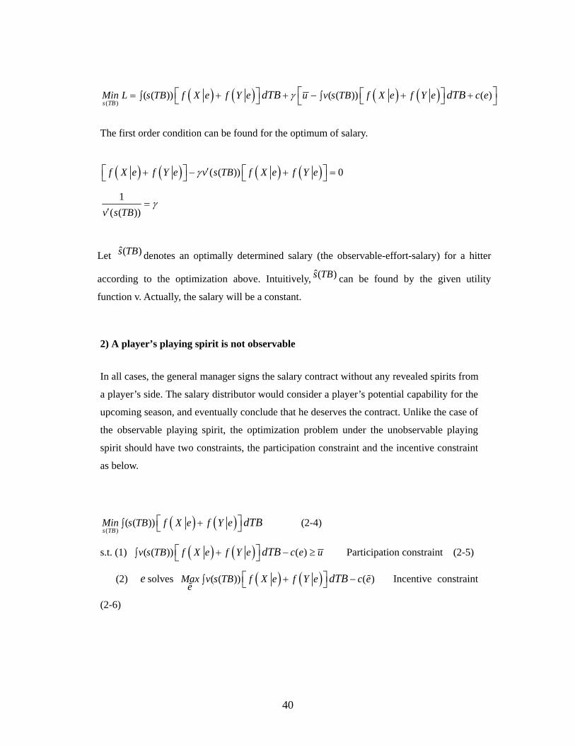
40
( ) ( ) ( ) ( )( )
( ( )) ( ( )) ( )s TBMin L s TB f X e f Y e u v s TB f X e f Y e c edTB dTBγ= + + − + +∫ ∫⎡ ⎤⎡ ⎤ ⎡ ⎤⎣ ⎦ ⎣ ⎦⎣ ⎦
The first order condition can be found for the optimum of salary.
( ) ( ) ( ) ( )( ( )) 0f X e f Y e v s TB f X e f Y eγ ′+ − + =⎡ ⎤ ⎡ ⎤⎣ ⎦ ⎣ ⎦
1( ( ))v s TB
γ=′
Let ˆ( )s TB denotes an optimally determined salary (the observable-effort-salary) for a hitter
according to the optimization above. Intuitively, ˆ( )s TB can be found by the given utility
function v. Actually, the salary will be a constant.
2) A player’s playing spirit is not observable
In all cases, the general manager signs the salary contract without any revealed spirits from
a player’s side. The salary distributor would consider a player’s potential capability for the
upcoming season, and eventually conclude that he deserves the contract. Unlike the case of
the observable playing spirit, the optimization problem under the unobservable playing
spirit should have two constraints, the participation constraint and the incentive constraint
as below.
( ) ( )( )
( ( ))s TBMin s TB f X e f Y e dTB+∫ ⎡ ⎤⎣ ⎦ (2-4)
s.t. (1) ( ) ( )( ( )) ( )v s TB f X e f Y e c e udTB+ − ≥∫ ⎡ ⎤⎣ ⎦ Participation constraint (2-5)
(2) e solves ( ) ( )( ( )) ( )Max v s TB f X e f Y e c ee
dTB+ −∫ ⎡ ⎤⎣ ⎦ %%
Incentive constraint
(2-6)

41
By the incentive contraint, a hitter would have a reason to play under one playing spirit
rather than under the other playing spirit.
3) Implementing a state Si for higher total base
An owner would implement either state of ‘Egoism’ or ‘Altruism’ from hitters.
{ },S AL EGi ∈ where AL denotes ‘Altruism’, and EG denotes ‘Egoism’. The incentive
constraint is follows.
( ) ( ) ( ) ( )( ( )) ( ) ( ( )) ( )i i i i i iv s TB f X S f S c S v s TB f X S f S c SY dTB Y dTB− − −− ≥ −∫ ∫⎡ ⎤ ⎡ ⎤+ +⎣ ⎦ ⎣ ⎦
The given incentive constraint, an owner finds the optimal salary for a hitter as below.
( ) ( ) ( ) ( )( ( )) ( ( )) ( )( ) i i i i iMin L s TB f X S f S u v s TB f X S f S c S
s TBY dTB Y dTBγ= + − +∫ ∫⎡ ⎤⎡ ⎤ ⎡ ⎤+ +⎣ ⎦ ⎣ ⎦⎣ ⎦
( ) ( ) ( ) ( )( ( )) ( ) ( ( )) ( )i i i i i iv s TB f X S f S c S v s TB f X S f S c SY dTB Y dTBμ − − −+ − − +∫ ∫⎡ ⎤⎡ ⎤ ⎡ ⎤+ +⎣ ⎦ ⎣ ⎦⎣ ⎦(2-8)
The first order condition can be found as below.
( ) ( ) ( ) ( )( ( ))i i i if X S f S v s TB f X S f SY Yγ ′−⎡ ⎤ ⎡ ⎤+ +⎣ ⎦ ⎣ ⎦
( ) ( ) ( ) ( ) ( ( )) 0i i i if X S f S f X S f S v s TBY Yμ − − ′+ − =⎡ ⎤⎡ ⎤ ⎡ ⎤+ +⎣ ⎦ ⎣ ⎦⎣ ⎦ (2-9)
Due to the incentive constraint, the derived condition seems to be different from the
derived condition under an observable playing spirit.
42
( ) ( )( ) ( )
11
( ( ))i i
i i
f X S f S
v s TB f X S f S
Y
Yγ μ
− −= + −
′
⎡ ⎤⎡ ⎤+⎣ ⎦⎢ ⎥⎡ ⎤+⎢ ⎥⎣ ⎦⎣ ⎦
(2-10)
The simplified condition actually represents that the optimal salary under an unobservable
playing spirit is not constant. As mentioned before, the optimal salary under an observable
playing spirit is constant. Unlike the optimal salary under a revealed spirit, this case
intuitively informs that the salary would depend on the probability densities of products.
ˆ( )s TB denotes an optimal salary under an observable playing spirit ( ˆ(1/ ( ( )))v s TB γ′ = ).
( ) ( )( ) ( )
1i i
i i
f X S f S
f X S f S
Y
Y− −
<⎡ ⎤+⎣ ⎦⎡ ⎤+⎣ ⎦
⇒ γ μ γ+ > ⇒1 1
ˆ( ( )) ( ( ))v s TB v s TB>
′ ′ (2-11)
⇒ ˆ( ( )) ( ( ))v s TB v s TB′ ′< ⇒ ˆ( ) ( )s TB s TB>
The salary under an unobservable playing spirit is greater than the salary under an
observable playing spirit if ( ) ( ) ( ) ( )i i i if X S f S f X S f SY Y− −>+ +
There are four cases for the inequality above.
1) ( ) ( )i if X S f X S−> , ( ) ( )i if S f SY Y −> ⇒ ˆ( ) ( )s TB s TB> : Impossible
2) ( ) ( )i if X S f X S−> , ( ) ( )i if S f SY Y −< ⇒Ambiguous
3) ( ) ( )i if X S f X S−< , ( ) ( )i if S f SY Y −> ⇒Ambiguous
4) ( ) ( )i if X S f X S−< , ( ) ( )i if S f SY Y −< ⇒ ˆ( ) ( )s TB s TB< : Impossible
In fact, the first and the fourth cases are impossible. A hitter can not have larger probability
densities for both a single and a big hit at one state than at the other state. So, we focus
only on the second and the third cases.

43
For the second case,
ˆ( ) ( )s TB s TB> if ( ) ( )i if X S f X S−− is greater than ( ) ( )i if S f SY Y −− .
This is true only when an owner implements a state of ‘Altruism’ because a probability
density of a single at ‘Altruism’ should be larger than at ‘Egoism’, and a probability
density of a big hit at ‘Egoism’ should be larger than at ‘Altruism’. Inexpensive players are
not very talented to make a big hit so an owner considers them to produce more singles. A
hitter lightly swings to make on-base by a spirit for a team’s winning more than a desire
for his own record. So, he can make a timely single for a leadoff or a run.
For the third case,
ˆ( ) ( )s TB s TB> if ( ) ( )i if S f SY Y −− is greater than ( ) ( )i if X S f X S−− .
This is true only when an owner implements a state of ‘Egoism’. From an owner’s view,
expensive players are efficient to make a big hit. In this case, they are exempted from the
spirit of ‘Altruism’. To produce a big hit, a batter desirously swings to fly a ball away so it
raises a probability of ‘Out’. In a state of ‘Egoism’, expensive hitters are expected to
produce more total bases. This is the reason why an owner implements a state of ‘Egoism’
for expensive hitters.
B. Slugger’s Choice in a ‘Component Sequential game’
Unlike other sports, baseball is a huge sequential game, which is comprised of a lot of
small component games between a hitter and a pitcher. Total base is recorded in two ways,
for a team and for an individual. An increase in individual’s total base implies an
improvement in team’s total base. This is why a ‘component game’ plays an important role.
By the incentive scheme, expensive hitters would concentrate on self-discipline to make
more total bases. When a slugger is at bat, a ‘component game’ starts by a pitcher’s throw.
A slugger can choose a strategy, ‘Swing Light’, ‘Swing Hard’, or ‘Don’t Swing’. For
simplicity, a strategy of ‘Swing Light’ can produce only a single with higher probability.
By ‘Swing Hard’, a hitter can make various outputs. He may not swing for a pitched ball.
Then, it possibly adds a strike-ball count.
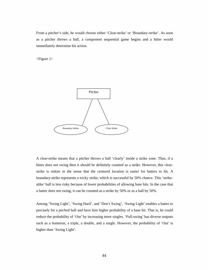
44
From a pitcher’s side, he would choose either ‘Clear-strike’ or ‘Boundary-strike’. As soon
as a pitcher throws a ball, a component sequential game begins and a hitter would
immediately determine his action.
<Figure 1>
A clear-strike means that a pitcher throws a ball ‘clearly’ inside a strike zone. Thus, if a
hitter does not swing then it should be definitely counted as a strike. However, this clear-
strike is riskier in the sense that the centered location is easier for batters to hit. A
boundary-strike represents a tricky strike, which is successful by 50% chance. This ‘strike-
alike’ ball is less risky because of lower probabilities of allowing base hits. In the case that
a batter does not swing, it can be counted as a strike by 50% or as a ball by 50%.
Among ‘Swing Light’, ‘Swing Hard’, and ‘Don’t Swing’, ‘Swing Light’ enables a batter to
precisely hit a pitched ball and have him higher probability of a base hit. That is, he could
reduce the probability of ‘Out’ by increasing more singles. ‘Full-swing’ has diverse outputs
such as a homerun, a triple, a double, and a single. However, the probability of ‘Out’ is
higher than ‘Swing Light’.
Pitcher
Boundary-Strike Clear-Strike

45
<Figure 2> In a subgame that a pitcher throws a ‘Boundary-Strike’
<Figure 3> In a subgame that a pitcher throws a ‘Clear-Strike’
Batter
Light-Swing
Full-Swing
Don’t Swing
SI 0.6
OUT 0.4
HR 0.08 TR
0.02DU 0.1
OUT 0.6
SK 1
BL 0
SI 0.2
Batter
Light-Swing
Full-Swing
Don’t Swing
SI 0.4
OUT 0.6
HR 0.05 TR
0.01DU 0.06
OUT 0.7
SK 0.5
BL 0.5
SI 0.18
46
<Figure 2> represents a batter is situated in a subgame when a pitcher throws a ‘Boundary-
Strike’. The indicated values below the final outputs inform the probability densities.
According to the densities, a batter has an expected base of 0.4 from ‘Swing Light’, an
expected base of 0.53(=0.05*4+0.01*3+0.06*2+0.18*1) from ‘Swing Hard’, and an
expected base of 0.125 (=0.5/4) from ‘Don’t swing’. Thus, a Nash Equilibrium strategy
should be ‘Swing Hard’ for a batter in the situation that a pitcher throws a ‘Boundary-
Strike’.
Similarly, <Figure 3> shows a batter’s subgame when a pitcher tries a ‘Clear-Strike’. By
the given probability densities with the final outputs, an expected base from ‘Swing Light’
is 0.6, and an expected base from ‘Swing Hard’ is 0.78 (= 0.08*4+0.02*3+0.1*2+0.2*1).
‘Don’t swing’ has 0. In this case, a strategy ‘Swing Hard’ is a Nash equilibrium strategy in
the subgame. For a pitcher’s reduced game, ‘Boundary-Strike’ should be a Nash
equilibrium strategy because he prefers less expected base. Thus, the SPNE is ((a pitcher
throws ‘Boundary-Strike’) and (a batter chooses ‘Swing Hard’)). An expected base is 0.5.
Intuitively, a pitcher already knows that a batter is going to swing hard since ‘Swing Hard’
should be a Nash equilibrium strategy in either subgame displayed above. All pitchers try
to reduce allowed bases by tricky strikes as possible. Even in unfavorable situation, a
batter swings hard because he knows that ‘Swing hard’ is still better than ‘Swing Light’ in
any situation. Basically, the SPNE tells how uncertainty of total base is deepened and how
baseball entertains fans. Despite a pitcher’s effort to prevent any bases, a batter is still able
to achieve bases. In fact, most slugger’s remarkable records are achieved under
challenging situation of many tricky balls.
In summary, the uncertainty of total base is even more increased due to a hitter’s sequential
game-theoretic situation.
C. Valuation of Outputs after a Season
As mentioned, each ‘component sequential game’ constitutes an entire baseball game. Due
to a Nash equilibrium chosen for an expected base, final outputs will be still randomly
distributed by their probability densities. Since an owner implements ‘Egoism (Self-
47
discipline)’ from expensive hitters for larger expected total bases, he would assess
sluggers’ achievements by focusing on big hits. At least, he will compare sluggers’ records
and what they are already paid. An owner will consider those records for the next contracts.
In this context, he has his own valuation method.
First of all, one can think that an owner develops a salary function as a weighted average
over all possible outputs, homeruns, triples, doubles, and singles. The following equation
represents what an owner would have in his mind.
4
1i i
i
X
Y eα
==∑
(3-1)
Y denotes a batter’s salary, 1X the number of homeruns, 2X the number of triples, 3X
the number of doubles and 4X the number of singles.
4
1ln i i
iY Xα
== ∑ (3-2)
Simply, the preference of base hit can be found as 4 (homerun) > 3 (triple) > 2 (double) > 1
(single) according to the order. First, an argument about contribution makes a homerun
have more weight in the salary equation because the advantage of automatic runs. Unlike
other types of base hits, a homerun automatically scores by itself. For example, a triple or a
double requires at least another statistical event to make a run. Second, a homerun mostly
excites fans. In most cases, people remember the homerun records and the famous
homerun hitter such as, Babe Ruth, Hank Aaron, and Barry Bonds. Even, media
continuously reports or forecasts who will possibly replace the on-going Homerun record
of Bonds based on the projected results. The mentioned hitters are Alex Rodriguez (New
York Yankees), David Ortiz (Boston Redsox), Albert Pujols (Saint Luis Cardinals), Manny
Ramirez (L.A. Dodgers), Ryan Howard (Philadelphia Phillies), and so on. If one hitter is in
a homerun race for a season or for his entire career, baseball fans would have more
interests on their team and would be more tempted to join ball games. A good homerun
hitter actually brings a positive shock on a team to raise the total revenue.

48
Furthermore, an owner would strongly prefer a homerun in the situation that a batter has a
limited capacity to hit bigger hits. Usually, a hitter’s total number of at-bats is
approximately restricted so the number of homeruns is supposed to decrease in the number
of other base hits. So, the more ‘emphasis’ on homeruns is supposed to be true in salary
equation above.
Given capacity 100, a hitter can allocate his capacity for three types of big hits by efforts.
For example, a good homerun hitter allocates 50% of capacity for homeruns, 10% for
triples, and 40% for doubles. One can find that there exists proximity among big hits. In
this case, the proximity between homeruns and triples is higher than that between
homeruns and doubles. Intuitively, it means that the triples could have been a homerun by
a little stronger impact. However, a double would not have been a homerun by the same
impact. For this hitter, a double needs an additional strength to become a homerun.
Conclusively, the athlete records fewer homeruns as he hits more triples. An opportunity
cost would follow a triple due to a stressed weight on a homerun. In the same manner, an
opportunity cost can be found from a double.
Considering the proximities, the function (3-2) can be rewritten as (3-3).
1 1 2 3 2 2 3 3 4 4ln ( , )Y X X X X X Xα α α α= + + + (3-3)
In (3-3), 1X (Homerun) depends on both 2X (Triple) and 3X (Double). An implication is that
the number of homerun should be affected by the number of triples and doubles under a
limited capacity. In the same sense, the number of triples or doubles would depend on the
number of homeruns. However, a homerun has no opportunity cost at this moment because
of the order of preference. In fact, an owner does not concern any proximity except for the
proximities affecting the number of homeruns.
The followings are obtained by taking a derivative with respect to 1X , 4X , 2X , and 3X .
11
lnd YdX
α= (3-4)

49
44
lnd YdX
α= (3-5)
12 1
2 2
ln Xd YdX X
α α∂
= +∂
where 1
2
0XX∂
<∂
(3-6)
1
2
0XX∂
<∂
implies that triples have a negative effect on homeruns under a limited capacity.
Intuitively, a negative effect informs that the proximity exists between a triple and a
homerun. According to (3-6), an overall effect of triples on a salary is composed of two
effects, a direct effect ( 2α ) and an indirect effect that is represented by the coefficient ( 1α )
times the proximity ( 1
2
XX∂
∂). If an indirect effect dominates a direct effect, then an overall
effect could be theoretically negative although a triple acquires three bases. An
interpretation is that triples’ total return is not sufficient to cover its cost of losing
homeruns from an owner’s view since the proximity represents an opportunity cost.
13 1
3 3
ln Xd YdX X
α α∂
= +∂
where 1
3
0XX∂
<∂
(3-7)
1
3
0XX∂
<∂
shows that the number of homeruns are negatively related the number of doubles
under a limited capacity. As similar as triples, an actual effect of doubles on salaries is
made up of two parts, which are a direct effect ( 3α ) and an indirect effect ( 11
3
XX
α∂
∂). The
implication is the same as the case of triples. However, it is presumed that the proximity
between doubles and homeruns is smaller than the proximity between triples and
homeruns. Accordingly, a direct effect is supposed to outweigh an indirect effect so a

50
positive effect of doubles on a salary would be expected. An implication is that a double
contributes the same as a triple with less opportunity cost so an owner is ready to
positively accept a double since it does not substantially hurt the number of homeruns.
1 1
2 3
X XX X∂ ∂
>∂ ∂
(3-8)
The inequality (3-8) shows that the proximity between triples and homeruns is greater than
the proximity between doubles and homeruns. More details will be discussed by empirical
findings in the next chapter.
Empirically, 1X must be an endogenous variable since it depends on both 2X and 3X
in (3-3). Thus, the variable of homerun should be treated as an endogenous variable in a
regression analysis. Without considering an endogenous property, a simple regression must
produce some errors. 2SLS estimation is suggested due to an endogenous variable.
3. Empirical Findings
A. American League
Data description 28 hitters and 289 observations
Each player has the same number of observations as his career years.
Gary Shaffield has the longest career by 17 years (1989-2006), and Justin Morneau has the shortest
career by 3 years (2004-2006).
To investigate determining factors of salaries, the variable of Salary could be regressed
onto all types of base hits including the variable of Homerun.
Salary X uβ= + where [ ] 5NX Con Single Double Triple Homerun
×= (4-1)
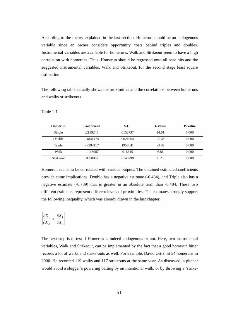
51
According to the theory explained in the last section, Homerun should be an endogenous
variable since an owner considers opportunity costs behind triples and doubles.
Instrumental variables are available for homeruns. Walk and Strikeout seem to have a high
correlation with homeruns. Thus, Homerun should be regressed onto all base hits and the
suggested instrumental variables, Walk and Strikeout, for the second stage least square
estimation.
The following table actually shows the proximities and the correlations between homeruns
and walks or strikeouts.
Table 1-1
Homerun Coefficient S.E. t-Value P-Value
Single .2139245 .0152737 14.01 0.000
Double -.4841474 .0621964 -7.78 0.000
Triple -.7394117 .1957041 -3.78 0.000
Walk .113987 .016615 6.86 0.000
Strikeout .0898962 .0143799 6.25 0.000
Homerun seems to be correlated with various outputs. The obtained estimated coefficients
provide some implications. Double has a negative estimate (-0.484), and Triple also has a
negative estimate (-0.739) that is greater in an absolute term than -0.484. These two
different estimates represent different levels of proximities. The estimates strongly support
the following inequality, which was already drawn in the last chapter.
1 1
2 3
X XX X∂ ∂
>∂ ∂
The next step is to test if Homerun is indeed endogenous or not. Here, two instrumental
variables, Walk and Strikeout, can be implemented by the fact that a good homerun hitter
records a lot of walks and strike-outs as well. For example, David Ortiz hit 54 homeruns in
2006. He recorded 119 walks and 117 strikeouts at the same year. As discussed, a pitcher
would avoid a slugger’s powering batting by an intentional walk, or by throwing a ‘strike-

52
alike’ ball, which is actually fishing a batter.
A pitcher implements the subgame perfect equilibrium strategy by pitching a ‘strike-alike’
ball according to the theory in the previous section. The derived SPNE supports that
expensive hitters prefer ‘Swing Hard’ to ‘Swing Light’, and batters actually have strike-
outs more times because of their attempts to put an exceedingly strong impact on a pitched
ball. This physically overwhelming effort raises a possibility of a strike-out. Thus, walks
and strike-outs can be good instrumental variables for homeruns. For implementing these
instrumental variables, the residual should be obtained through the regression (4-2) as
below.
Homerun Zα ε= + (4-2)
where [ ] 5NZ Single Double Triple Walk Strikeout
×=
Eventually, the variable ‘Salary’ will be regressed onto all the explanatory variables
including the residuals obtained from the regression (4-2) as above.
ˆSalary X uβ γε= + + (4-3)
The null hypothesis 0 : 0H γ = is tested. By rejecting the null hypothesis, it can be
concluded that Homerun is endogenous. The test result is as follows.
Table1-2
Ln_Salaries1 Coefficient S.E t-Value P-Value
Single .0016813 .0047315 0.36 0.723
Double .0115548 .013084 0.88 0.378
Triple -.093309 .037516 -2.49 0.013
Homerun .0297622 .0105339 2.83 0.005
Residual .0379959 .0167703 2.27 0.024
Constant 12.87462 .2012876 63.96 0.000

53
Apparently, the null hypothesis of 0 : 0H γ = should be rejected by the obtained results.
Homerun is concluded as an endogenous variable. Furthermore, the test results inform that
a simple OLS would result in some errors. Therefore, the second stage estimation is
recommended to avoid any errors. However, both test results will be provided cohesively
for a comparison and a contrast in this research.
1) With a simple OLS
The test results are as follows.
Table1-3
Ln_Salaries1 Coefficient S.E t-Value P-Value
Single .0086116 .0036362 2.37 0.019
Double .0004604 .012222 0.04 0.970
Triple -.1145622 .0365905 -3.13 0.002
Homerun .0447534 .0082566 5.42 0.000
Constant 12.86299 .2026966 63.46 0.000
The relatively smaller hits such as singles and doubles lead to very small estimates 0.009
and 0.0005 for Single and Double, respectively. However, the relatively bigger bits, triples
and homeruns have bigger estimates. Remarkably, there is a huge difference between an
estimate for Double and that for Triple in an absolute value. The question is if the
abnormally big difference between two estimates rises from the errors, and the difference
would be reduced by 2SLS.
2) With a 2SLS
The second stage estimation shows the results in the following table. Comparing to the
OLS, the estimated coefficients seem to be aligned by 2SLS estimation. That is, the

54
estimates for Double and Homerun are actually increased, but the estimate for Triple is
decreased in an absolute term.
Table1-4
Ln_Salaries1 Coefficient S.E t-Value P-Value
Single .0016813 .0048315 0.35 0.728
Double .0115548 .0133607 0.86 0.388
Triple -.093309 .0383094 -2.44 0.015
Homerun .0677582 .013325 5.09 0.000
Constant 12.87462 .2055443 62.64 0.000
Different from the OLS, the p-value of Single substantially rises from 0.019 to 0.728 by
2SLS. The p-value of Double falls to 0.388, and the p-value of Triple rises to 0.015.
However, the estimate of Triple is still significant. By either estimation, Homerun is most
significant.
Table 1-4 exhibits an interesting result that the p-values are actually arranged in an order
by Single, Double, Triple and Homerun. That is, Homerun is most significant in
determining the salary with the estimated coefficient, 0.068. The second is Triple with the
estimated coefficient, -.093. The third is Double with the estimate, 0.012, and the fourth is
Single with 0.002.
Notably, the most significant variable, Homerun, has the largest positive estimated
coefficient, and Double has the second. Single has the third. Triple has the negative
estimate.
All of these estimates indicate that an owner concentrates on homeruns rather than any
other types of hits at his decision for a hitter’s salary. According to the test result, Double
has a positive effect on a salary however it is insignificant. Triple has a negative impact on
a salary with sufficient significance even though a triple acquires more bases than a double
or a single. It seems that a double is strictly preferred to a triple. An insignificant positive
estimate of Double implies that doubles do not play any negative roles in salary. Moreover,
its insignificance might imply zero effect on a salary. In another word, doubles would
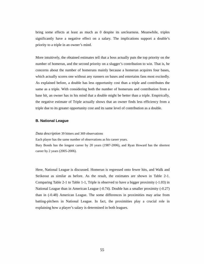
55
bring some effects at least as much as 0 despite its unclearness. Meanwhile, triples
significantly have a negative effect on a salary. The implications support a double’s
priority to a triple in an owner’s mind.
More intuitively, the obtained estimates tell that a boss actually puts the top priority on the
number of homerun, and the second priority on a slugger’s contribution to win. That is, he
concerns about the number of homeruns mainly because a homerun acquires four bases,
which actually scores one without any runners on bases and entertains fans most excitedly.
As explained before, a double has less opportunity cost than a triple and contributes the
same as a triple. With considering both the number of homeruns and contribution from a
base hit, an owner has in his mind that a double might be better than a triple. Empirically,
the negative estimate of Triple actually shows that an owner finds less efficiency from a
triple due to its greater opportunity cost and its same level of contribution as a double.
B. National League
Data description 39 hitters and 369 observations
Each player has the same number of observations as his career years.
Bary Bonds has the longest career by 20 years (1987-2006), and Ryan Howard has the shortest
career by 2 years (2005-2006).
Here, National League is discussed. Homerun is regressed onto fewer hits, and Walk and
Strikeout as similar as before. As the result, the estimates are shown in Table 2-1.
Comparing Table 2-1 to Table 1-1, Triple is observed to have a bigger proximity (-1.03) in
National League than in American League (-0.74). Double has a smaller proximity (-0.27)
than in (-0.48) American League. The some differences in proximities may arise from
batting-pitchers in National League. In fact, the proximities play a crucial role in
explaining how a player’s salary is determined in both leagues.

56
Table 2-1
Homerun Coefficient S.E. t-Value P-Value
Single .1910018 .0178108 10.72 0.000
Double -.2701738 .0640572 -4.22 0.000
Triple -1.031126 .1553716 -6.64 0.000
Walk .1381923 .012932 10.69 0.000
Strikeout .057763 .0109794 5.26 0.000
Also, the bigger estimated coefficient (0.14) for Walk and the smaller estimated coefficient
(0.06) for Strikeout are found in Table 2-1, compared to Table 2-1(0.11 and 0.09,
respectively for Walk and Strikeout). Baseball fans acknowledge a reason. Traditionally,
both leagues are mainly different by the designated hitting system, which allows one hitter
not to join in fielding. American League accepts the designated hitting rule but National
League does not. Thus, all fielders including a pitcher have to join a batting line-up in
National League. In this case, there exits the weakest spot in the line-up because of a
pitching-hitter so an opponent team’s pitcher can intentionally walk power hitters more
times to face a pitching-hitter in National League. Sluggers tend to have more walks and
fewer strike-outs in National League than in American League.
Under the presumption that Homerun is an endogenous variable, Salary is regressed onto
all other explanatory variables including the residuals obtained from the simple OLS above.
The test results are contained in the following Table 2-2.
Table 2-2
Ln_Salaries1 Coefficient S.E t-Value P-Value
Single -.0050084 .0051403 -0.97 0.331
Double .027438 .012578 2.18 0.030
Triple -.0413302 .0348975 -1.18 0.237
Homerun .0231364 .009739 2.38 0.018
Residual .0418539 .0177585 2.36 0.019
Constant 13.23069 .1802799 73.39 12.87617

57
There is no big difference for the estimated coefficient for Residual between Table 1-2
(0.038) and Table 2-2 (0.042). It is largely because the effect from the bigger estimate of
Walk has been offset by the effect from the smaller estimate of Strikeout in National
League. Accordingly, Residual has the low P-value (0.019), which sufficiently supports the
significance of the estimate (0.042). Thus, Homerun is concluded as an endogenous
variable.
1) With a simple OLS
By the endogenous variable of Homerun, 2SLS method is recommended to prevent any
errors from occurring in estimation. However, a simple OLS estimation results are
provided for comparison and contrast.
Table 2-3
Ln_Salaries1 Coefficient S.E t-Value P-Value
Single .0032037 .0038026 0.84 0.400
Double .0193204 .0121727 1.59 0.113
Triple -.0814523 .0306536 -2.66 0.008
Homerun .0357242 .0081946 4.36 0.000
Constant 13.19992 .1809281 72.96 0.000
By a simple OLS, Triple seems to have the biggest effect on a salary by the negative
estimate (-0.081) with the P-value of 0.008. Homerun has the second biggest effect by the
positive estimate (0.036) with P-value of 0.000. Double has the third biggest effect
however the estimate is not significant (p-value of 0.113). Interestingly, the estimated
coefficient of Homerun is much smaller than the estimate of Triple in an absolute term.
The problem may rise from the endogenous Homerun.
2) With a 2SLS
The estimators should be biased and inconsistent by a simple OLS largely because of one
endogenous variable. Instead, the 2SLS estimation results follow in Table 2-4.
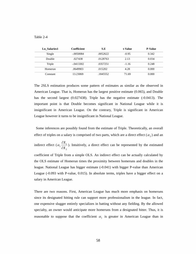
58
Table 2-4
Ln_Salaries1 Coefficient S.E t-Value P-Value
Single -.0050084 .0052622 -0.95 0.342
Double .027438 .0128763 2.13 0.034
Triple -.0413302 .0357251 -1.16 0.248
Homerun .0649903 .015202 4.28 0.000
Constant 13.23069 .1845552 71.69 0.000
The 2SLS estimation produces some pattern of estimates as similar as the observed in
American League. That is, Homerun has the largest positive estimate (0.065), and Double
has the second largest (0.027438). Triple has the negative estimate (-0.0413). The
important point is that Double becomes significant in National League while it is
insignificant in American League. On the contrary, Triple is significant in American
League however it turns to be insignificant in National League.
Some inferences are possibly found from the estimate of Triple. Theoretically, an overall
effect of triples on a salary is comprised of two parts, which are a direct effect ( 2α ) and an
indirect effect ( 11
2
XX
α∂
∂). Intuitively, a direct effect can be represented by the estimated
coefficient of Triple from a simple OLS. An indirect effect can be actually calculated by
the OLS estimate of Homerun times the proximity between homeruns and doubles in the
league. National League has bigger estimate (-0.041) with bigger P-value than American
League (-0.093 with P-value, 0.015). In absolute terms, triples have a bigger effect on a
salary in American League.
There are two reasons. First, American League has much more emphasis on homeruns
since its designated hitting rule can support more professionalism in the league. In fact,
one expensive slugger entirely specializes in batting without any fielding. By the allowed
specialty, an owner would anticipate more homeruns from a designated hitter. Thus, it is
reasonable to suppose that the coefficient 1α is greater in American League than in
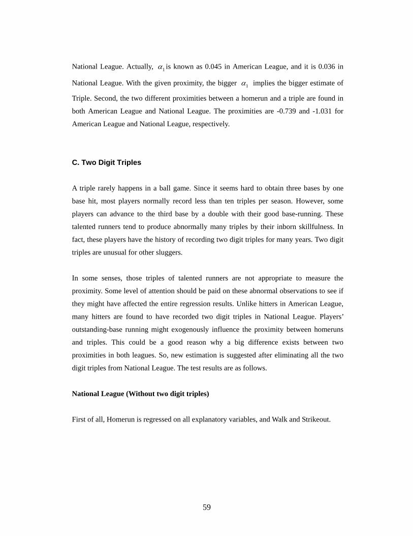
59
National League. Actually, 1α is known as 0.045 in American League, and it is 0.036 in
National League. With the given proximity, the bigger 1α implies the bigger estimate of
Triple. Second, the two different proximities between a homerun and a triple are found in
both American League and National League. The proximities are -0.739 and -1.031 for
American League and National League, respectively.
C. Two Digit Triples
A triple rarely happens in a ball game. Since it seems hard to obtain three bases by one
base hit, most players normally record less than ten triples per season. However, some
players can advance to the third base by a double with their good base-running. These
talented runners tend to produce abnormally many triples by their inborn skillfulness. In
fact, these players have the history of recording two digit triples for many years. Two digit
triples are unusual for other sluggers.
In some senses, those triples of talented runners are not appropriate to measure the
proximity. Some level of attention should be paid on these abnormal observations to see if
they might have affected the entire regression results. Unlike hitters in American League,
many hitters are found to have recorded two digit triples in National League. Players’
outstanding-base running might exogenously influence the proximity between homeruns
and triples. This could be a good reason why a big difference exists between two
proximities in both leagues. So, new estimation is suggested after eliminating all the two
digit triples from National League. The test results are as follows.
National League (Without two digit triples)
First of all, Homerun is regressed on all explanatory variables, and Walk and Strikeout.
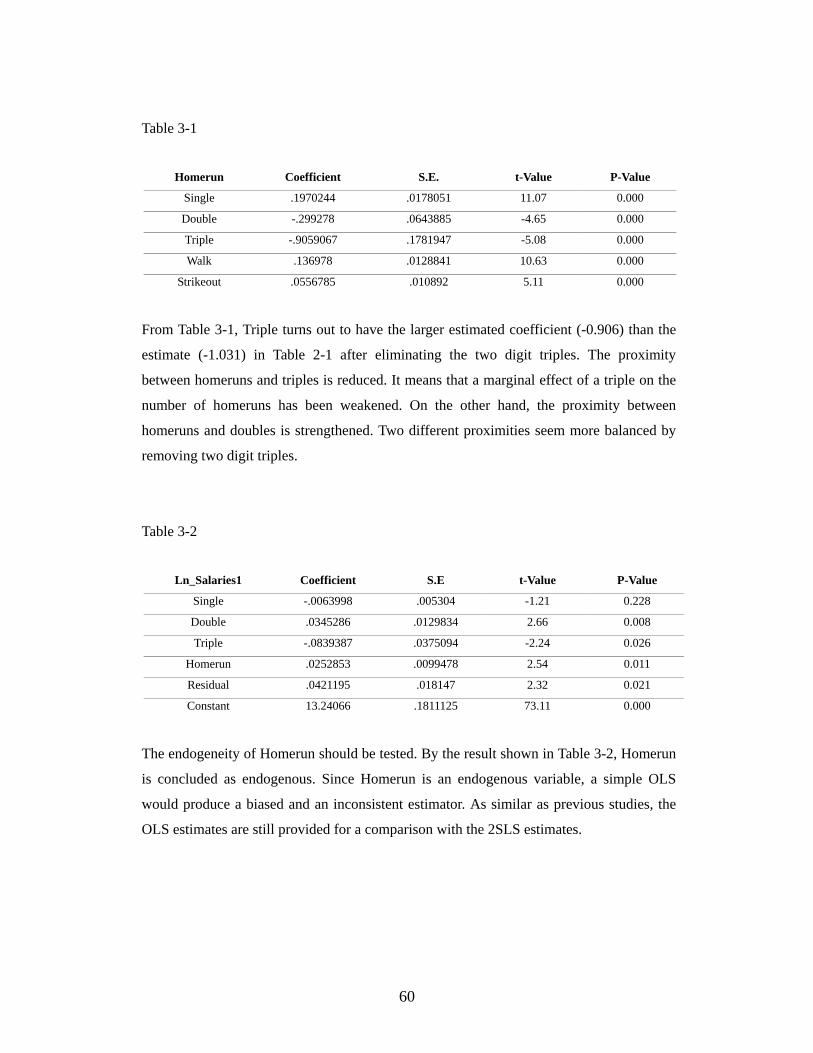
60
Table 3-1
Homerun Coefficient S.E. t-Value P-Value
Single .1970244 .0178051 11.07 0.000
Double -.299278 .0643885 -4.65 0.000
Triple -.9059067 .1781947 -5.08 0.000
Walk .136978 .0128841 10.63 0.000
Strikeout .0556785 .010892 5.11 0.000
From Table 3-1, Triple turns out to have the larger estimated coefficient (-0.906) than the
estimate (-1.031) in Table 2-1 after eliminating the two digit triples. The proximity
between homeruns and triples is reduced. It means that a marginal effect of a triple on the
number of homeruns has been weakened. On the other hand, the proximity between
homeruns and doubles is strengthened. Two different proximities seem more balanced by
removing two digit triples.
Table 3-2
Ln_Salaries1 Coefficient S.E t-Value P-Value
Single -.0063998 .005304 -1.21 0.228
Double .0345286 .0129834 2.66 0.008
Triple -.0839387 .0375094 -2.24 0.026
Homerun .0252853 .0099478 2.54 0.011
Residual .0421195 .018147 2.32 0.021
Constant 13.24066 .1811125 73.11 0.000
The endogeneity of Homerun should be tested. By the result shown in Table 3-2, Homerun
is concluded as endogenous. Since Homerun is an endogenous variable, a simple OLS
would produce a biased and an inconsistent estimator. As similar as previous studies, the
OLS estimates are still provided for a comparison with the 2SLS estimates.

61
1) With a simple OLS
Table 3-3
Ln_Salaries1 Coefficient S.E t-Value P-Value
Single .0020497 .0038811 0.53 0.958
Double .0252138 .0124235 2.03 0.043
Triple -.1181063 .0347119 -3.40 0.001
Homerun .0379424 .0083711 4.53 0.000
Constant 13.20513 .1815728 72.73 0.000
As seen in Table 3-3 above, the estimates of all the base hits are found to diminish after
eliminating two digit triples. The estimate of Triple is actually decreased (increased in an
absolute term). Here, the argument is focused more on a marginal effect of a base hit on a
salary so the changes in estimates have interpretations that marginal effects of base hits
have been affected by removing two digit triples. In fact, it indicates that two digit triples
have played some roles in the regression results. Homerun has quite a small estimated
coefficient 0.038. The marginal effect of homeruns on a salary seems weak. The relatively
small effect strongly supports that the estimates are actually biased and inconsistent.
2) With a 2SLS
Table 3-4
Ln_Salaries1 Coefficient S.E t-Value P-Value
Single -.0063998 .0054286 -1.18 0.239
Double .0345286 .0132885 2.60 0.010
Triple -.0839387 .0383908 -2.19 0.029
Homerun .0674049 .015534 4.34 0.000
Constant 13.24066 .1853682 71.43 0.000
Usually, good base-runners show relatively many triples largely due to their techniques but
fewer homeruns, compared to other sluggers. It means that most of their triples would have

62
been a double to a normal-base-runner. However, the skillful hitters can obtain one more
base by their tactics and their timely run. This point was not taken into account in the
previous regressions. As a result, a triple seems to have less opportunity cost for a homerun.
In American League, the estimated coefficient of Triple is -0.093, and the estimate
substantially rises up to -0.041 in National League. Without two digit triples, the estimate
restore the lower level -0.084 in National League. As discussed, the changed estimates
insinuate that two digit triples of National League have affected the regression results.
4. Conclusion
‘Over-emphasis’ of homerun was the arguing point in the beginning of this research.
Different from other sports, higher payroll does not necessarily improve team
performances. Theoretically, owners hire expensive hitters and implement ‘Egoism (Self-
discipline)’ from those hitters to have larger expected total bases by increasing the number
of ‘big hits’ and by decreasing the number of singles. Thus, the uncertainty of total base
increases. At bats, the expensive hitters choose ‘Swing Hard’ in either case that a pitcher
throws a ‘Clear-strike’ or a ‘Boundary-strike’. In a sequential game, a pitcher throws a
‘Boundary-strike’ as the first mover. So, the uncertainty of total bases increases even more
by these strike-alike balls. When a season ends, an owner collects all hitter’s records,
reviews them, and compares them to his payments before he makes new contracts for the
next year. He must have his own salary function.
Empirically, an owner’s salary function is estimated by the second stage least square. As
the theory points out in section 2, owners totally disregard the number of singles to
determine expensive hitters in both American League and National League. The P-values
of Single are very high in both leagues. Meanwhile, bigger hits such as Homerun, Triple,
and Double have significant estimates. Specially, Homerun always has the largest positive
estimate in every case with 0 P-value. An implication is that the number of homeruns
makes a big impact on an owner’s decision for a salary. Double also has positive estimates
in all cases. The positive estimates of Homerun and Double support that owners actually
emphasize big hits and implement ‘Egoism (Self-discipline)’. Interestingly, Triple has
negative estimates in all cases. The negative estimate of Triple strongly supports that an
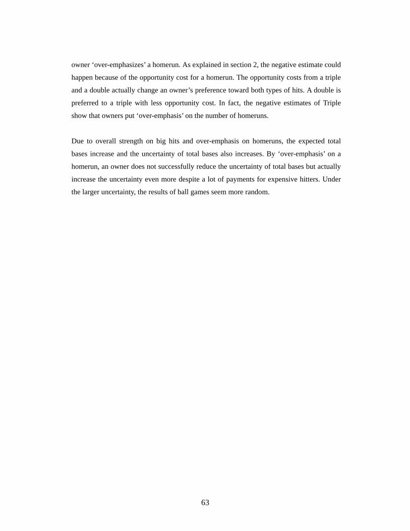
63
owner ‘over-emphasizes’ a homerun. As explained in section 2, the negative estimate could
happen because of the opportunity cost for a homerun. The opportunity costs from a triple
and a double actually change an owner’s preference toward both types of hits. A double is
preferred to a triple with less opportunity cost. In fact, the negative estimates of Triple
show that owners put ‘over-emphasis’ on the number of homeruns.
Due to overall strength on big hits and over-emphasis on homeruns, the expected total
bases increase and the uncertainty of total bases also increases. By ‘over-emphasis’ on a
homerun, an owner does not successfully reduce the uncertainty of total bases but actually
increase the uncertainty even more despite a lot of payments for expensive hitters. Under
the larger uncertainty, the results of ball games seem more random.
64
Chapter 3. Any Subsidy Converges to a Direct Quantity Control Over Infinite Horizon
1. Introduction
A subsidy and a direct quantity control are leading trade policies over many countries.
Many researchers have tried to figure out how these two main policies would support the
domestic exporters and, furthermore, develop national welfare since these policies are
mostly useful for helping domestic firms improve their profits. Interestingly, Cooper and
Riezman (1989) found a general conclusion under what condition one policy is more
useful than the other based on a game-theoretic approach. According to them, a subsidy is
a dominant policy when a foreign market is placed under a sufficiently large uncertainty.
The paper also shows that a dominant policy becomes a direct quantity control if
uncertainty reduces to a sufficiently lower level in a foreign market. The result intuitively
makes sense. Under no market uncertainty, an oligopolist reasonably would earn more
profit by a constrained quantity. However, it is unsure if a constrained quantity still helps
earn more profit under large demand variability. This is what Cooper and Riezman have
mainly found through their four-stage long sequential game frame.
An important question can be raised when we extent their results to an infinite horizon
model. That is, if we let the governments choose their policies through an infinite horizon
then the subsidy policy is not so efficient. For example, if a government individually
subsidizes exporters for every period infinite times then a social cost would be
substantially big although a future subsidy should be discounted. Instead, if the policy
makers reallocate a part of subsidy for infrastructure, in purpose, to stabilize demand
variability for their own exporters and successfully induce a direct quantity control then
the overall social cost could be saved.
This paper shows how a government improves total discounted social benefit by
reallocating a subsidy through an infinite horizon and any dominant subsidy policy is
changed to a direct quantity control over time. This paper eventually shows how the C-R

65
(referring Cooper and Riezman)’s SPNE, under the sufficiently large demand variability,
changes over time for two different cases, one-sided intervention and both-sided
intervention. In section 4, one-sided intervention represents that only one government
involves in the project of stabilizing demand. In this case, the SPNE changes only once
because one government actually changes its dominant policy to a quantity control by the
time that the demand variability is stabilized. The SPNE might change more than once if
both governments join the project of stabilizing demand.
In section 5, we discuss the both-sided intervention case. Depending on the number of
exporting firms, the SPNE would change only once or more than once. That is, if both
countries have the same number of exporting firms then the demand stability is realized at
the same time for both countries. Under this symmetric case, the SPNE would change only
once over time because both governments coincidentally choose a quantity control as a
dominant policy. Instead, if both countries have different number of exporting firms then
their demand stabilities are realized by the different timings because of asymmetric
condition. Under this asymmetric condition, the SPNE would change twice over time
because both governments differently change their dominant policies to a quantity control.
2. Foreign market under market uncertainty
According to Cooper and Riezman (1989), both governments involving trade policy game
face four stages to reach a final output. At the first stage, the two public authorities
determine an intervention mode. Secondly, the rivals decide intervention levels. At the
third, market uncertainty is revealed to the firms. Finally, the firms maximize their profits
with the given government’s intervention at the fourth stage. Most of all, the firms’ optimal
quantities under the given trade policies must be found in the fourth stage.
Cooper and Riezman introduced the concept of social benefit, the sum of all domestic
firms’ profits. By using the derived the optimal quantities in the fourth stage, an expected
social benefit function or formula can be investigated from a domestic government’s view.
The problem is to find the ex post subsidy that maximizes this expected social benefit.
66
Simply speaking, the policy makers need to find a Nash equilibrium of the reduced game
as an optimal subsidy. This Nash equilibrium actually represents the SPNE. The authors
have different SPNE according to the size of variance, which is denoted byθ . In fact,
when the variance of θ is sufficiently large, the government’s policy mode must be
chosen as a subsidy. When the variance of θ becomes sufficiently small, the
government’s policy mode should be chosen as a direct quantity control.
Intuitively, a government anticipates how domestic firms would obtain their profits from
the trade policy or it can be foreseen how the firms will be benefited by the selected
governmental service. To choose any policy, a government considers an expected social
benefit, the sum of all domestic firms’ expected profits.
The values below show the obtained expected social benefits in an oligopolistic situation
from both governments’ perspectives by Cooper and Riezman. According to the tables,
each government would reach an expected social benefit by choosing a trade police such
as a subsidy or a direct quantity control.

67
(Table 1) Expected social benefit for a Country 1’s firm from Cooper and Riezman (1989)
Country 2
Subsidies Quantities
Country1
Subsidies
2
22 2
1
( ) (1 ) ( )
( 3) ( 1)
a c N Var
bN F b F
θ− ++
+ +
2
2 21 1 1
( ) ( )
( 3) ( 1)
a c Var
bN N b N
θ−+
+ +
Quantities
2
22
1 2
( ) ( 1)
( 3)
a c N
bN N
− +
+
2
1
( )
9
a c
bN
−
(Table 2) Expected social benefit for a Country 2’s firm from Cooper and Riezman (1989)
Country 2
Subsidies Quantities
Country1
Subsidies
2
12 2
2
( ) (1 ) ( )
( 3) ( 1)
a c N Var
bN F b F
θ− ++
+ +
21
22 1
( ) ( 1)
( 3)
a c N
bN N
− +
+
Quantities
2
2 22 2 2
( ) ( )
( 3) ( 1)
a c Var
bN N b N
θ−+
+ +
2
2
( )
9
a c
bN
−

68
Both governments simultaneously select either subsidy or direct quantity control as a
policy mode, and four different sequential game starts with four nodes if the entire police
game is depicted. So, there are supposed to be four different expected social benefits in a
reduced form at which both governments choose their police modes. In a game theoretic
sense, the four-stage long extensive game has been reduced to a one-shot simultaneous
game by backward induction.
According to the expected social benefits matrix above, the SPNE is ((Policy mode is
Subsidy, Policy mode is Subsidy), ( *1s , *
2s ), (θ is revealed), ( *1q , *
2q )) when ( )Var θ is
sufficiently large. This SPNE changes to ((Policy mode is Direct Quantity Control, Policy
mode is Direct Quantity Control), ( **1q , **
2q ),(θ is revealed ), ( **1q , **
2q )) when ( )Var θ is
sufficiently small.
3. Expenditure for Infrastructure and Variance Assessment
Any exporting firms are supposed to encounter a substantial level of demand variability in
a newly developed foreign market. Sometimes, foreign customers have biased preferences
toward the origins of products or the nationalities. If they originate from the same country
then they are assumed to meet the same demand variability. Under a volatile demand, a
subsidy should be a dominant policy for both governments according to Cooper and
Riezman because a policy helps firms individually adjust to unstable circumstances.
However, if policy makers think over their choices under an infinite horizon, they would
realize that stabilizing market demand eventually helps improve their social benefit more
than subsidizing firms for every period. First, they assess demand variability and search for
any possibility to lower the variability for domestic firms. Accordingly, a government
spends some expenditure for infrastructure to stabilize demand.
For example, Korean government has a special institution such as KOTRA to bolster
domestic exporters, and the public institution has local agencies over many countries. Its
main objective is to help Korean firms have more information about a market or a local
area. In fact, highly skilled manpower performs a high quality of research about a market
69
and regularly has an open seminar in which consumer reports and market details are
covered. In some cases, they are requested a market survey or forecasting. Since KOTRA
successfully achieved its goal of supporting Korean exporters over all countries, some
local governments of Korea have their own institutions or facilities to benefit mid-sized
firms originating from their local provinces these days.
Korean exporting firms used to be provided a financial support (a subsidy) for their
exported products. However, they are more benefited from well-founded governmental
agencies over the world. Intuitively, Korean firms would become oligopolists when they
eventually have stable demand, and they are suggested to constrain the exported quantity
for raising their profitability.
1) Variance Assessment
A government collects all information about a market and concludes that the demand
variability could be overcome by a public-led effort. The variance of iθ is a decreasing
function of expenditure for infrastructure ( 1g ) such as 2( )i i iVar kgθ σ= − . As mentioned,
the market level of variance is a sum of all individual levels of variances such
as1
( ) ( )N
ii
Var Varθ θ=
= ∑ . This idea is from the total demand1
N
ii
Q q=
= ∑ . The variance of total
demand is constituted of the variances of individual demands such as 1
( ) ( )N
ii
Var Q Var q=
= ∑ .
Products are originated from different countries so the differently-originated products
would face different demand variabilities due to prejudices for their origins. For example,
Japanese cars, Korean mobile phones. Customers usually generalize a product’s quality by
its origin.

70
2) Expenditure for infrastructure
A government actually spends some expenditure ( 1g ) on establishing public infrastructure
within a limited budget ( *1 10 g s< < ).
4. Onesided Intervention
Here, only one government has a motivation to lower demand variability for helping its
domestic firms by a public infrastructure. In the following section, two different
governments simultaneously establish a public infrastructure for their own domestic firms.
Formally, government 1 reallocates the pre-determined budget *1s for subsidy into 1s (a
subsidy for exported good) and 1g (expenditure for infrastructure). That is, *1 1 1s s g= + .
Simply speaking, government 1 finds the optimal value, *1g , maximizing the total
expected discounted social benefit by reducing the demand variability to the efficient level
under the constraint, *1 1 1s s g= + .
However, government 2 spends no expenditure for infrastructure ( 2 0g = ) because of no
reallocated subsidy. Thus, *2 2s s= .
As government 1 spends some money for infrastructure over time to bring demand stability,
a stable demand becomes present earlier. Importantly, Cooper and Riezman have not
provided the information about the value of variance by which an unstable demand could
be turned into a stable demand. A government would recognize ‘by chance’ that the
individual variability for its domestic firms has been sufficiently reduced. A stable demand
is assumed to arrive by exponential probability density.
A government’s expenditure for infrastructure affects the timing of a stable demand. If 1g
denotes an instantaneous spending for infrastructure by government 1 then the instant
success rate for realization of a stable demand, u is 1( )gα . The time of occurrence of

71
u is denoted as uτ , which is exponentially distributed with a density function.
1( )1( ) ( ) ug
u u g e α τψ τ α −= , 0 uτ< < ∞
The dominance of a subsidy policy still remains until 1θ ’s variance diminishes to the
sufficiently small level. As mentioned, the value of the sufficiently small variance is still
unknown. Implicatively, a public-led effort can not stop due to unawareness of the
boundary of variance although the variance continuously diminishes. Rather, a government
would recognize an arrival of a stable demand for its domestic firms by chance.
Once individual demand variability is sufficiently reduced, a direct quantity control
becomes a dominant policy for a government while the rival still chooses a subsidy policy.
The SPNE changes by the timing of a stable demand for country 1.
As mentioned before, government 1 takes a part ( 1g ) from the pre-determined level ( *1s )
and reallocates for each period. With expenditure for infrastructure ( 01g > ), the new
expected social benefit can be found as follows.
2
' * * 21 1 1 1 1 2 2 2
1
1( )( ) (1 )
( 3) ( 1)( ( , 0), )
Vara c N
bN F b FE s s s g s
θπ
′− ++
+ +′= > =
+ 22 1 21 1
( )(1 ) 1
( 1)( 3) ( 1) ( 1)
a c N bN Ng g
b F F b F b F
− + +−
+ + + +
⎡ ⎤ ⎡ ⎤ ⎡ ⎤⎢ ⎥ ⎢ ⎥ ⎢ ⎥⎣ ⎦ ⎣ ⎦ ⎣ ⎦
where 1 1s s′ < and 21 1( )Var kgθ σ′ = −

72
With an increased expenditure ( 1g ) for infrastructure, an individual-financial support
(subsidy) level for an exported product should be reduced, and ( )Var θ continuously
diminishes for every time period while the government’s overall expenditure ( *1 1s s g= + )
for domestic firms should remain the same.
* * * * 11 1 1 1 1 2 1 1 2 2( , )
( 1)( ( , 0), ) kg
E s sb F
E s s s g s ππ −+
′ ′= > =
22 1 21 1
( )(1 ) 1
( 1)( 3) ( 1) ( 1)
a c N bN Ng g
b F F b F b F
− + +−
+ + + +
⎡ ⎤ ⎡ ⎤ ⎡ ⎤+ ⎢ ⎥ ⎢ ⎥ ⎢ ⎥⎣ ⎦ ⎣ ⎦ ⎣ ⎦
* * * *
1 1 2 1 1 1 1 1 2( , ) ( ( , 0), )E s s E s s s g sπ π− ′ ′= >
=
2 11 2 21 1 2
1 ( )(1 )
( 1) ( 1) ( 1)( 3) ( 1)bN N a c N
g gb F b F b F F
kgb F
− ++ − +
+ + + + +⎡ ⎤ ⎡ ⎤ ⎡ ⎤⎢ ⎥ ⎢ ⎥ ⎢ ⎥⎣ ⎦ ⎣ ⎦ ⎣ ⎦
As a subsidy is reduced, total social benefit decreases. Interestingly, the marginal change
of total social benefit from reducing a subsidy and establishing infrastructure can be
minimized for each period. With continuous spending for demand stability, a stable
demand will be realized. However, the timing of a stable demand is randomly distributed
as mentioned. By an arrival of a stable demand, two separate stages (the Initial Stage and
Stage One) can be defined. In the Initial Stage, a government still spends some money for
infrastructure to bring a stable demand and no firms have a stable demand. The Initial
Stage continues until demand stability is achieved by government 1’s support. By an
occurrence of demand stability, the Initial Stage changes to Stage One. Both governments
have different total expected social welfares in each stage. At first, the total expected
discounted social benefits in Stage One for both governments can be found.

73
1) In Stage One
In Stage One, the demand variability remains sufficiently small for the firms originating
from country 1. A stable demand is assumed to take place at t N= . However, the firms
originating from the other country still face larger demand variability.
By the timing of a stable demand, government 1 would deviate from a subsidy to a direct
quantity control. By government 1’s deviation, both governments face the new expected
social benefits as below. By referring to the expected social benefit matrix (Table 1) and
(Table 2),
** *1 1 2( , )E q sπ =
22
21 2
( ) ( 1)
( 3)
a c N
bN N
− +
+
** *2 1 2( , )E q sπ =
22
2 22 2 2
( )( )
( 3) ( 1)
Vara c
bN N b N
θ−+
+ +
Government 2 still has a dominant policy of a subsidy because2
( )Var θ has never changed.
Actually, the new bilateral game starts at t N= and new social benefits are ** *1 1 2( , )E q sπ
and ** *2 1 2( , )E q sπ for country 1 and country 2, respectively, in every time period. By
comparing ** *1 1 2( , )E q sπ and ** *
2 1 2( , )E q sπ , an interesting point can be found. Unlike
country 1, the variance plays a major role in the new social benefit for country 2. It
ironically supports that a subsidy policy is proper under larger uncertainty and the firms
from country 2 still has larger demand variability. An intuition is that total social welfare
for country 2 has larger uncertainty while total social welfare for country 1 has less
uncertainty.
With a government-supported infrastructure, a trade policy converges to a direct quantity
control. A government always considers the best policy for its own domestic exporters.
Under an unstable demand, a subsidy helps domestic firms most efficiently because funded
firms can individually adjust to dynamic market circumstances. Meanwhile, a direct
74
quantity control policy must be more efficient under a stable demand. In fact, oligopoly
firms tend to sell smaller amount at a higher price for larger total revenue in a market. This
is the main reason why a government chooses a direct quantity control as a dominant
policy under demand stability.
Let *,1H N denote the government 1’s total expected discounted social welfare at t N= .
** *
* ** * 1 1 2,1 1 1 2
0
( , )( , )N
E q srtH e E q s dtr
ππ
∞ −= =∫
Let *,2H N denote the government 2’s expected discounted total social welfare at t N= .
** ** ** * 2 1 2
,2 2 1 20
( , )( , )N
E q srtH e E q s dtr
ππ
∞ −= =∫
2) In the Initial Stage
As remarked earlier, the Initial Stage lasts unless market uncertainty is removed, and
government 1 still spends expenditure for infrastructure to support domestic exporters. To
avoid any confusion, the Initial Stage is assumed to start at 0t = .
Let *0,1H denote government 1’s total expected discounted social benefit at 0t = . No
one knows when a stable demand is realized for the firms from country 1. A stable demand
causes a substantial change on an exporter’s profit and eventually on a government’s
expected discounted total social benefit. Government 1 is able to derive *0,1H by the
randomly distributed timing of a stable demand and its probability density function,
depending on 1g .
75
( )* * * ** *0,1 1 1 1 1 1 2 1 1 2
0 0( ( ( , 0), )) [ ( , ) ] ( )rt rtH e E s s s g s dt e E q s dt d
τ
τπ π ψ τ τ
∞ ∞− −′= = > +∫ ∫ ∫
⎡ ⎤⎢ ⎥⎣ ⎦
( )* * ** *1 1 1 1 1 2 1 1 2
0
1 1( ( , 0), ) 1 ( , ) ( )rt rtE s s s g s e e E q s d
r rπ π ψ τ τ
∞− −′ ′= = > − +∫
⎡ ⎤⎡ ⎤⎣ ⎦⎢ ⎥⎣ ⎦
* * ** *
1 1 1 1 1 2 1 1 1 1 2
1 1
( ( , 0), ) ( ) ( ) ( , )1
( ) ( )
E s s s g s g g E q sr r g r g r
π α α πα α
′ ′= >= − +
+ +
⎡ ⎤ ⎡ ⎤⎡ ⎤ ⎡ ⎤ ⎡ ⎤⎣ ⎦⎢ ⎥⎢ ⎥ ⎢ ⎥ ⎢ ⎥
⎣ ⎦⎣ ⎦ ⎣ ⎦⎣ ⎦
where 11
( )( ) ( ) gg e α τψ τ α −= , *1 10 g s< < ,
1
1 1( ) kg gα⎛ ⎞⎜ ⎟⎝ ⎠=
Thus, * * *
1 1 1 1 1 2 1 ,1*0,1
1
( ( , 0), ) ( )[ ]
( )NE s s s g s g H
Hr g
π α
α
′ ′= > +=
+, where
** ** 1 1 2
,1( , )
NE q sH
rπ
=
2
* * 21 1 1 1 1 2 2 2
1
1( )( ) (1 )
( 3) ( 1)( ( , 0), )
Vara c N
bN F b FE s s s g s
θπ
− ++
+ +′ ′= > =
+ 22 1 21 1
( )(1 ) 1
( 1)( 3) ( 1) ( 1)
a c N bN Ng g
b F F b F b F
− + +−
+ + + +
⎡ ⎤ ⎡ ⎤ ⎡ ⎤⎢ ⎥ ⎢ ⎥ ⎢ ⎥⎣ ⎦ ⎣ ⎦ ⎣ ⎦
Interestingly, government 1 can determine the optimal level of 1g in each period. The
intuition is that when the government reduces an individual financial support (a subsidy)
and allocates the reduction for a public infrastructure the expected social welfare is not
linearly decreased. As mentioned before, a marginal decrease of the expected social benefit
from reducing a subsidy could be minimized.
76
1
* * * *1 1 2 1 1 1 1 1 2( , ) ( ( , 0), )
gE s sMin E s s s g sπ π− ′ ′= >
where * * * *1 1 2 1 1 1 1 1 2( , ) ( ( , 0), )E s s E s s s g sπ π− ′ ′= >
= 2 11 2 21 1 2
1 ( )(1 )
( 1) ( 1) ( 1)( 3) ( 1)bN N a c N
g gb F b F b F F
kgb F
− ++ − +
+ + + + +⎡ ⎤ ⎡ ⎤ ⎡ ⎤⎢ ⎥ ⎢ ⎥ ⎢ ⎥⎣ ⎦ ⎣ ⎦ ⎣ ⎦
2
*1
1 2
2( 1)
( )(1 )
( 1)( 3)
2 1
( 1) ( 1)
k
b F
a c N
b F F
bN N
b F b F
g−
+
− +
+ +
+
+ +
⎡ ⎤⎢ ⎥⎣ ⎦=⎡ ⎤ ⎡ ⎤⎢ ⎥ ⎢ ⎥⎣ ⎦ ⎣ ⎦
With government 1’ optimal expenditure ( *1g ) for infrastructure, the instant success rate is
determined. As government 1 spends a determined expenditure to reduce 1( )Var θ for
more time periods, the probability of reaching a stable demand rises.
Country 1’s total expected social welfare can be calculated as follows.
1
* * * *1 1 1 1 1 2 1 ,1*
0,1 1*1
( ( , 0), ) ( ) [ ]
( )
kN
k
E s s s g s g HH
r g
π ′ ′= > +=
+
where2 2 *
* * 2 11 1 1 1 1 2 2 2
1
( ) (1 )
( 3) ( 1)( ( , 0), )
a c N
bN F b FE s s s g s
kgπ
σ− ++
+ +′ ′= > =
−
+ ( )2*2 1 2 *11
( )(1 ) 1
( 1)( 3) ( 1) ( 1)g
a c N bN Ng
b F F b F b F
− + +−
+ + + +
⎡ ⎤ ⎡ ⎤ ⎡ ⎤⎢ ⎥ ⎢ ⎥ ⎢ ⎥⎣ ⎦ ⎣ ⎦ ⎣ ⎦

77
Let *0,2H denote government 2’s total expected discounted social benefit at 0t = .
( )* * * * ** *0,2 2 1 1 1 1 2 2 1 2
0 0( ( , 0), ) , ( )rt rtH e E s s s g s dt e E q s dt d
τ
τπ π ψ τ τ
∞ ∞− −′ ′= = > +∫ ∫ ∫
⎡ ⎤⎡ ⎤⎡ ⎤⎣ ⎦ ⎣ ⎦⎢ ⎥⎣ ⎦
where ( )11( ) ( ) gg e α τψ τ α −=
1* * * * *
2 1 1 1 1 2 1 ,2*0,2 1
*1
( ( , 0), ) ( ) [ ]
( )
kN
k
E s s s g s g HH
r g
π ′ ′= > +=
+
where ( )* ** *
2 1 2*,2
,N
E q sH
r
π=
( )2 2 2
* * * * *1 1 1 12 1 1 1 1 2 2 2 1 122
1( ) (1 ) ( ) ( )(1 )1 ( 3) 1( 3) ( 1)
( ( , 0), )b
a c N Var N a c N Ng gF bN F FbN F b F
E s s s g sθ
π⎡ ⎤⎡ ⎤ ⎡ ⎤+⎢ ⎥⎢ ⎥ ⎢ ⎥⎣ ⎦ ⎣ ⎦⎣ ⎦
− + − ++ ++ + ++ +
′ ′= > =
Since the optimal choice of expenditure for infrastructure is made by government 1, SPNE
should be revised for each period.
The SPNE, ((Policy mode is Subsidy, Policy mode is Subsidy), ( *1s , *
2s ), ( 1θ and 2θ are
revealed), ( *1q , *
2q )), lasts until a stable demand is realized for the firms from country 1.
Then it turns to New SPNE, ((Policy mode is Direct quantity control, Policy mode is
Subsidy), ( **1q , *
2s ), ( 1θ and 2θ are revealed and 1( )Var θ turns out to be sufficiently
small), ( **1q , *
2q )).
This SPNE remains forever.
5. Bothsided Intervention
Only one government has been discussed so far. Here, both governments simultaneously
reduce their levels of subsidies for increasing total social benefits under infinite horizon.
They do prefer less uncertainty of total social welfare so stabilizing demand for their
domestic firms would help. There are two different cases, symmetry and asymmetry. The

78
symmetry supports that both countries have equal number of firms in a foreign market.
The asymmetry represents the case that one country has larger number of firms than the
other country in a foreign market. Thus, demand variability for the firms from the country
should be larger than demand variability for the firms from the other country. A stable
demand takes more time in this case.
1. Symmetric case ( 1 2N N N= = )
This case represents that both countries would have equal number of firms in a foreign
market. Unlike the asymmetric case, Nash equilibrium expenditure for infrastructure is
identical for both governments. An intuition is that both governments’ choices would be
the same under the same circumstances. The identical choices lead all the firms to have a
stable demand at the same time regardless their origins since the instant success rates
become the same in this case.
As similar as the asymmetric case, there are two different stages, Initial Stage and Stage
One. In the Initial Stage, both governments spend money for infrastructure and a stable
demand is not realized in this stage. This stage maintains until both governments
successively stabilize the demands for their own domestic firms. By the timing of
stabilizing demands, the Initial Stage changes into Stage One. No governments spend
money for infrastructure in Stage one since a stable demand coincidentally happens for all
the firms regardless the origins.
1) Stage One
Both governments stop spending for infrastructure. By stable demands for all the firms
from both origins, both governments would change a trade policy from a subsidy to a
direct quantity control. In this stage, the total expected discounted social benefits for both
governments are as follows. It is assumed that stable demands happen for the firms from
both countries at t N= .

79
Let *,1H N denote the government 1’s total expected discounted social welfare at t N= .
** **
* ** ** 1 1 2,1 1 1 2
0
( , )( , )rt
NE q q
H e E q q dtr
ππ
∞−= =∫
Let *,2H N denote the government 2’s total expected discounted social welfare at t N= .
** **
* ** ** 2 1 2,2 2 1 2
0
( , )( , )rt
NE q q
H e E q q dtr
ππ
∞−= =∫
2) The Initial Stage
In this stage, no stable demand has been realized for the firms from either country. Both
governments continuously spend money for infrastructure to reduce the market variances
for their own domestic firms. By backward induction, the entire sequential game can be
reduced to the Initial Stage. Both governments’ total expected discounted social benefits
are found as below.
Let *0,1H denote the government 1’s total expected discounted social welfare at 0t = .
( ) ( )1
1
* ** **0,1 1 1 1 2 2 1 1 2 1 1
0 0( , ) ( )( ), ( )rt rtH e dt e E q q dE s g s g
τ
τπ ψ τ τπ
∞ ∞− −= +∫ ∫ ∫
⎡ ⎤′ ′ ′⎡ ⎤⎣ ⎦⎢ ⎥⎣ ⎦
( )[ ]
( )1 1 1 2 2 1 1 1 2 2** **
1 1 1 2
1
( ), ( ) ( ), ( )( ) ( , )( )
E s g s g E s g s gg E q qr r g r r
π πα πα
′ ′ ′ ′ ′ ′⎡ ⎤= + −⎢ ⎥+ ⎣ ⎦
Let *0,2H denote the government 2’s total expected discounted social welfare at 0t = .

80
( ) ( )2
2
* ** **0,2 2 1 1 2 2 2 1 2 2 2
0 0( , ) ( )( ), ( )rt rtH e dt e E q q dE s g s g
τ
τπ ψ τ τπ
∞ ∞− −= +∫ ∫ ∫
⎡ ⎤′ ′ ′⎡ ⎤⎣ ⎦⎢ ⎥⎣ ⎦
( )[ ]
( )2 1 1 2 2 2 1 1 2 22 2
2
** **1 2( ), ( ) ( ), ( )( ) ( , )
( )E s g s g E s g s gg E q q
r r g r rπ πβ π
β′ ′ ′ ′ ′ ′⎡ ⎤
= + −⎢ ⎥+ ⎣ ⎦
where 21( ) ( )g gα β=
In determining the optimal expenditure for infrastructure, both governments would face
the simultaneous game situation. As reviewed in one-sided intervention case, when a
government cuts a subsidy to support infrastructure then a marginal decrease of the
expected social welfare can be minimized. In this context, Nash Equilibrium ( )* *1 2,g g
can be found.
Due to the expenditures for infrastructure, both governments reduce subsidies as below.
*i i is s g′ = − where
( )(1 )*( 3)
i ii
i
a c N Ns
N F−− − −
=+
for 1, 2i =
The corresponding quantities are found as follows.
* 2 21 1 1 2
1
( 1) ( 1)
N Nq q g g
b F b F
+′ = − +
+ +
⎡ ⎤⎢ ⎥⎣ ⎦
* 1 12 2 2 1
1
( 1) ( 1)
N Nq q g g
b F b F
+′ = − +
+ +
⎡ ⎤⎢ ⎥⎣ ⎦
where ( )(1 )*
( 3) ( 1)i i
ii
a c Nq
bN F b F
θ−− += +
+ + for 1, 2i =

81
Both firms’ new social welfare functions are derived as below.
* * 1 1 2 2 2 2 21 1 2 1 1 2 1 21 2
1
( ) ( )( )(1 ) 1
( , ) ( , )1 ( 3) ( 1) ( 1)
g gN g N g a c N N N
E s s E s s g gF bN F b F b F
π π+ − + +
′ ′ ′ = + − ++ + + +
⎡ ⎤⎛ ⎞⎡ ⎤⎢ ⎜ ⎟ ⎥⎢ ⎥⎣ ⎦ ⎝ ⎠⎣ ⎦
* * 1 1 2 2 1 1 12 2 2 1 2 2 11 1 2
2
( ), ( )( )(1 ) 1
( ) ( , )1 ( 3) ( 1) ( 1)
gN g N g a c N N N
E s g s E s s g gF bN F b F b F
π π+ − + +
′ ′ ′ = + − ++ + + +
⎡ ⎤⎛ ⎞⎡ ⎤⎢ ⎜ ⎟ ⎥⎢ ⎥⎣ ⎦ ⎝ ⎠⎣ ⎦
where 2 2
* *1 2 2
( ) (1 )( , )
( 3) ( 1)
( )i i ii
i
a c N kgE s s
bN F b F
σπ −− + −
= ++ +
for 1, 2i =
By minimizing the marginal decrease of total social benefits from the reduced subsidy,
Nash Equilibrium ( )* *1 2,g g can be found.
From the first order condition, ( ) ( )* *
1 11 2 1 1 2 2
1
0, ( ), ( )d E E
dg
s s s g s gπ π⎡ ⎤⎢ ⎥⎣ ⎦
′−=
′ ′
21 1 2 1 2 1 2 2
1
( )(1 )( 1) 2 (1 ) ( 1 ) 0
( 3)
a c Nk b F N N N g N N N g
bN F
− +− + + − + + − − =
+
From the first order condition ( ) ( )* *
2 21 2 1 1 2 2
2
0, ( ), ( )d E E
dg
s s s g s gπ π⎡ ⎤⎢ ⎥⎣ ⎦
′−=
′ ′
12 2 1 2 1 2 1 1
2
( )(1 )( 1) 2 (1 ) ( 1 ) 0
( 3)
a c Nk b F N N N g N N N g
bN F
− +− + + − + + − − =
+
Under the symmetric condition 1 2N N= , each government considers that its rival would
make the same choice as itself.
* *1 2
( )( 1)(1 )
( 3)
2 (1 )
a c F Nk
Fg g
N N
− + +−
+= =
+
⎡ ⎤⎢ ⎥⎣ ⎦

82
The equilibrium total expected discounted social benefits for both governments are found
as below, and they are actually equal.
( ) ( )* * * **1 1 1 2 2 1 1 1 2 2** 1
0,1 *1
** **1 1 2
( ), ( ) ( ), ( )( ) ( , )( )
E s g s g E s g s gg E q qHr r rr g
π πα πα
⎡ ⎤′ ′ ′ ′ ′ ′⎢ ⎥= + −
⎡ ⎤+ ⎢ ⎥⎣ ⎦ ⎣ ⎦
( ) ( )* * * **2 1 1 2 2 2 1 1 2 2** 2 2
0,2 *2
** **1 2
( ), ( ) ( ), ( )( ) ( , )( )
E s g s g E s g s gg E q qHr r rr g
π πβ πβ
⎡ ⎤′ ′ ′ ′ ′ ′⎢ ⎥= + −
⎡ ⎤+ ⎢ ⎥⎣ ⎦ ⎣ ⎦
Thus, ** **0,1 0,2H H=
The SPNE, ((Policy mode is Subsidy, Policy mode is Subsidy), ( *1s , *
2s ), ( 1θ and 2θ are
revealed), ( *1q , *
2q )), lasts until a stable demand is realized for the firms from country 1.
Then it turns to New SPNE, ((Policy mode is Direct quantity control, Policy mode Direct
quantity control), ( **1q , **
2q ), ( 1θ and 2θ are revealed, and 1( )Var θ and
2( )Var θ coincidentally turn out to be sufficiently small), ( **1q , **
2q )).This SPNE remains
forever.
2. Asymmetric case (the number of firms from country 2 is greater than the number of
firms from country 1, 2 1N N> )
In this case, a stable demand for the firms from country 1 should be realized earlier than
country 2. There are also two different stages, Initial stage and Stage One, by the timing of
a stable demand for country 1.
1) Stage One
Government 1 spends nothing for infrastructure since a stable demand for firms from
country 1 was already realized in the past. However, a stable demand for the other country

83
is still in a process so government 2 spends for infrastructure. In this stage, total social
benefits for both countries can be found as below.
First, government 1 would consider two different instant social benefits ** *1 1 2( , )E q sπ and
** **1 1 2( , )E q qπ by the timing 2τ to calculate its overall social welfare as below.
( ) ( )2
2
* ** * ** **1 1 2 1 1 2 2 2,1
0 0( , ) ( , ) ( )rt rt
NH e E q s dt e E q q dt d
τ
τπ π ψ τ τ
∞ ∞− −= +∫ ∫ ∫
⎡ ⎤⎢ ⎥⎣ ⎦
The integral above actually represents its own expected discounted social benefit after
government 1 stabilizes demand for its own domestic firms and can be solved as follows
( ) ( ) 22** * ** * *
1 1 2 1 1 2 220
1 1( , ) 1 ( , ) ( )rrE q s e E q q e dr rττπ π ψ τ τ
∞−−⎡ ⎤
⎢ ⎥⎣ ⎦= − +∫ ⎡ ⎤⎢ ⎥⎣ ⎦
( ) ( ) ( )** * ** * ** **1 1 2 1 1 2 1 1 2
2 2
1 1 11 1( , ) ( , ) ( , )( ) ( )E q s E q s E q qr r rr g r gπ π πβ β⎡ ⎤ ⎡ ⎤⎢ ⎥ ⎢ ⎥⎢ ⎥ ⎢ ⎥⎣ ⎦ ⎣ ⎦
= − ++ +
Similarly, government 2 can find total social benefit as below. From government 2’s
perspective, its own demand stability would be realized no earlier than government 1’s.
After government 1’s demand stability at 1τ , government 2’s expected discounted social
benefit can be found by the integral as below.
( ) ( )2
2
* ** * ** **2 1 2 2 1 2 2 2,2
0 0( , ) ( , ) ( )rt rt
NH e E q s dt e E q q dt d
τ
τπ π ψ τ τ
∞ ∞− −= +∫ ∫ ∫
⎡ ⎤⎢ ⎥⎣ ⎦
( ) ( ) 22** * ** **
2 1 2 2 1 2 2 20
1 1( , ) 1 ( , ) ( )rtrE q s e E q q e dr rτπ π ψ τ τ
∞−−⎡ ⎤
⎢ ⎥⎣ ⎦= − +∫ ⎡ ⎤⎢ ⎥⎣ ⎦
( ) ( ) ( )** * ** * ** **2 1 2 2 1 2 2 1 2
2 2
1 1 11 1( , ) ( , ) ( , )( ) ( )E q s E q s E q qr r rr g r gπ π πβ β⎡ ⎤ ⎡ ⎤⎢ ⎥ ⎢ ⎥⎢ ⎥ ⎢ ⎥⎣ ⎦ ⎣ ⎦
= − ++ +

84
2) Initial Stage
As explained before, there two demand variability by different countries. Each government
can reduce its own demand variability by expenditure for infrastructure. Two different
governments would stabilize their demand variability at a different time. If government 1
successfully reduces the variance arising for the country 1 earlier than government 2 then
its total expected discounted social welfare can be calculated as follows.
( )1
1
* *,10,1 1 1 1 2 2 1 1
0 0( )( ), ( )rt rt
NH e dt e H dE s g s gτ
τψ τ τπ
∞ ∞− − ⎡ ⎤
⎢ ⎥⎣ ⎦= +∫ ∫ ∫⎡ ⎤′ ′ ′⎡ ⎤⎣ ⎦⎢ ⎥⎣ ⎦
where ( ) ( )* *1 1 1 2 2 1 1 1 1 2 2 21 2
( , 0), ( , 0)( ), ( ) E s s s g s s s gE s g s g ππ ′ ′ ′= = > = >′ ′ ′
That is, government 2 still tries to reduce the variance arising for the country 2 after
government 1 already has demand stability. By the randomly distributed timing 1τ ,
government 1 chooses **1q while the rival chooses *
2s . Later on, government 2 would
succeed in stabilizing its individual market demand by 2τ . It means that government 1’s
total expected social welfare will be changed from ** *1 1 2( , )E q sπ to ** **
1 1 2( , )E q qπ by
the timing 2τ .
So, government 1’s total expected discounted social welfare is derived as below.
*0,1H = ( )
*,1 2
1
11 1 1 2 2
1 1
[ ( )]( )1 ( )
( ) ( )( ), ( )
NH gg rgr r g r gE s g s g
βααα απ
⎡ ⎤⎡ ⎤⎢ ⎥⎢ ⎥⎢ ⎥⎢ ⎥⎡ ⎤ ⎣ ⎦⎢ ⎥⎢ ⎥ ⎢ ⎥⎢ ⎥⎣ ⎦ ⎢ ⎥⎢ ⎥⎣ ⎦
− ++ +
′ ′ ′⎡ ⎤⎣ ⎦

85
Similarly, government 2 can find its total expected discounted social welfare as below.
( )1
1
* *,20,2 2 1 1 2 2 1 1
0 0( )( ), ( )rt rt
NH e dt e H dE s g s gτ
τψ τ τπ
∞ ∞− − ⎡ ⎤
⎢ ⎥⎣ ⎦= +∫ ∫ ∫⎡ ⎤′ ′ ′⎡ ⎤⎣ ⎦⎢ ⎥⎣ ⎦
where ( ) ( )* *2 1 1 2 2 1 1 1 2 2 21 22 ( , 0), ( , 0)( ), ( ) E s s s g s s s gE s g s g ππ ′ ′ ′= = > = >′ ′ ′
Eventually, government 2’s total expected discounted social welfare is found as follows.
*0,2H = ( )
*,2 2
1
12 1 1 2 2
1 1
[ ( )]( )1 ( )
( ) ( )( ), ( )
NH gg rgr r g r gE s g s g
βααα απ
⎡ ⎤⎡ ⎤⎢ ⎥⎢ ⎥⎢ ⎥⎢ ⎥⎡ ⎤ ⎣ ⎦⎢ ⎥⎢ ⎥ ⎢ ⎥⎢ ⎥⎣ ⎦ ⎢ ⎥⎢ ⎥⎣ ⎦
− ++ +
′ ′ ′⎡ ⎤⎣ ⎦
Both governments’ total expected discounted social benefits are actually functions of
instant success rates, which depends on expenditures for infrastructure. To find the Nash
Equilibrium ( )* *1 2,g g , the first order conditions should be reconsidered.
From the first order condition, ( ) ( )* *
1 11 2 1 1 2 2
1
0, ( ), ( )d E E
dg
s s s g s gπ π⎡ ⎤⎢ ⎥⎣ ⎦
′−=
′ ′
21 1 2 1 2 1 2 2
1
( )(1 )( 1) 2 (1 ) ( 1 ) 0
( 3)
a c Nk b F N N N g N N N g
bN F
− +− + + − + + − − =
+
From the first order condition ( ) ( )* *
2 21 2 1 1 2 2
2
0, ( ), ( )d E E
dg
s s s g s gπ π⎡ ⎤⎢ ⎥⎣ ⎦
′−=
′ ′
12 2 1 2 1 2 1 1
2
( )(1 )( 1) 2 (1 ) ( 1 ) 0
( 3)
a c Nk b F N N N g N N N g
bN F
− +− + + − + + − − =
+

86
[ ]
2 11 1 2
*1
1 2 1 1 2 1 1 2
( )( 1)(1 ) ( )( 1)(1 )2(1 ) ( 1 )
( 3) ( 3)
4 (1 )(1 ) ( 1 ) ( 1 )
a c F N a c F NN k N N k
F Fg
N N N N N N N N
− + + − + ++ − + − − −
+ +=
+ + − − − − −
⎡ ⎤ ⎡ ⎤⎢ ⎥ ⎢ ⎥⎣ ⎦ ⎣ ⎦
1
* *1 2 12 1
2 1 2 1
( )( 1)(1 )
( 1 )( 3)
2 (1 ) 2 (1 )
a c F Nk
N N NFg g
N N N N
− + +−
− −+= +
+ +
⎡ ⎤⎢ ⎥⎣ ⎦
The equilibrium total expected discounted social benefits for both governments are follows.
**0,1H = ( )
* *,1 2*
1** * 1
1 1 2 * *1 1
2
[ ( )]( )1 ( )( ,
( ) ( )) ( )
NH gg rgE s g sr r g r gg
βααπα α
⎡ ⎤⎡ ⎤⎢ ⎥⎢ ⎥⎢ ⎥⎢ ⎥⎡ ⎤ ⎣ ⎦⎢ ⎥⎢ ⎥⎢ ⎥⎢ ⎥⎣ ⎦ ⎢ ⎥⎢ ⎥⎣ ⎦
′ ′ ′ − ++ +
⎡ ⎤⎣ ⎦
**0,2H = ( )
*,2
* *1 2
*2*
1*1
2 1 2 * *1 1
[ ( )]( )1 ( ),
( ) ( )( ) ( )
N gg
g
g g
Hr
E s sr r rg g
βααπα α
⎡ ⎤⎡ ⎤⎢ ⎥⎢ ⎥⎢ ⎥⎡ ⎤ ⎢ ⎥
⎣ ⎦⎢ ⎥⎢ ⎥⎢ ⎥⎢ ⎥
⎣ ⎦ ⎢ ⎥⎢ ⎥⎣ ⎦
′ ′ ′ − ++ +
⎡ ⎤⎣ ⎦
The Nash Equilibrium tells that both firms spend a determined expenditure for every
period however the timing of demand stability is still random. By their expenditures, the
total social welfares would be expected.
The SPNE, ((Policy mode is Subsidy, Policy mode is Subsidy), ( *1s , *
2s ), ( 1θ and 2θ are
revealed), ( *1q , *
2q )), lasts until a stable demand is realized for the firms from country 1.
Then it turns to New SPNE, ((Policy mode is Direct quantity control, Policy mode is
Subsidy), ( **1q , *
2s ), ( 1θ and 2θ are revealed, and 1( )Var θ turns out to be sufficiently
small), ( **1q , *
2q )). This SPNE lasts until a stable demand is realized for the firms from

87
country 2. Then it turns to New SPNE, ((Policy mode is Direct quantity control, Policy
mode Direct quantity control), ( **1q , **
2q ), ( 1θ and 2θ are revealed, and 2( )Var θ turns out
to be sufficiently small), ( **1q , **
2q )).This SPNE remains forever.
6. Conclusion
The argument has been centered on if a dominant trade policy should converge to a direct
quantity control under infinite horizon. The answer was ‘yes’ because a government has a
vision to improve total social benefit for infinite horizon and might be ready to take a loss
of total social benefit occurring from a reduction of a subsidy for some periods. As a result,
the demand variability is successively reduced while the firms from the other country still
struggle with large demand variability. Under a government-led effort to remove the
market variance, government 1 has a dominant policy of direct quantity control. The rival
government still chooses a subsidy as dominant policy since the demand variability for its
domestic exporters are unchanged. Under the new dominant equilibrium policies, the total
expected discounted social benefits for country 1 and country 2 can be compared. Unlike
country 1, country 2 has large uncertainty for its total expected discounted social benefit.
In the sense of less uncertainty, the total social benefit for country 1 is more efficient.
If both governments involve in the removal of market variance, there would be two
different cases, the symmetry and the asymmetry. In the symmetric case, both firms have
equal number of firms in a market. Intuitively, both governments have the same choices
under the identical circumstances. Thus, stable demands for all the firms coincidentally
happen regardless the origins. In this case, the dominant equilibrium trade policy changes
from (subsidy, subsidy) to (direct quantity control, direct quantity control). The total
expected discounted social benefits for both governments can be found in this sense. They
are actually equal.
In the asymmetric case, each country has different number of firms operating in a market.
For example, if country 2 has larger number of firms than country 1 then it would take
more time for government 2 to stabilize demand for all the firms. Accordingly, government

88
2 successively stabilizes the demands for its own domestic exporter after government 1
succeeded. In this situation, the total expected discounted social benefits for both
governments can be obtained. Unlike the symmetric case, the dominant equilibrium trade
policy changes from (subsidy, subsidy) to (direct quantity control, subsidy). Depending on
government 2’s expenditure for infrastructure, the equilibrium changes to (direct quantity
control, direct quantity control) again.

89
References
Allen, F. (1985), “Repeated Principal-Agent Relationship with Lending and Borrowing,”
Economic Letters, 17:23-31
Angrist, J.D (1990), “Lifetime Earnings and the Vietnam Era Draft Lottery: Evidence from
Social Security Administrative Records.” American Economic Review. 80: 313-336.
Angrist, J.D. and W. N. Evans (1998), “Children and Their Parents’ Labor Supply:
Evidence from Exogenous Variation in Family Size.” American Economic Review. 88:45-
477.
Angrist, J.D., G.W. Imbens, and D.B. Rubin (1996), “Identification of Causal Effects
Using Instrumental Variables.” Journal of the American Statistical Association, 91:444-455.
Angrist, J. and A. Krueger (1991), “Does Compulory School Attendance Affect Schooling
and Earnings?” Quarterly Journal of Economics 106:979-1014.
Angrist, J. and A. Krueger (1999), “Empirical Strategies in Labor Economics,” Chapter 23
in Handbook of Labor Economics (Vo.3), ed. Orley Ashenfelter and David Card. Elsevier,
1278-1329.
Arvan, L. (1991), “Flexibility versus Commitment in Strategic Trade Policy under
Uncertainty,” Journal of International Economics, 31:341-355
Bagwell, K., and R. W. Staiger (1994), “The Sensitivity of Strategic and Corrective R&D
Policy in Oligopolistic Industries,” Journal of International Economics 36(December):
136-150
Bound, J., D.A. Jaeger, and R.M. Baker (1995), “Problems with Instrumental Variables
Estimation When the Correlation Between Instruments and the Endogenous Explanatory
Variable is Weak,” Journal of the American Statistical Association, 90:443-450.
90
Bhattacharya, G. (1986), “Innovation Games in Vertical Markets,” mimeo, University of
Kansas.
Brander, J.A. and B.J. Spencer (1983), “Strategic Commitment with R&D: The Symmetric
Case,” Bell Journal of Economics, 14(1):225-235
Brander, J.A. and B.J. Spencer (1985), “Export subsidies and International Markets Share
Rivalry,” Journal of International Economics, 18:83-100
Brainard, S. L. and D. Martimort (1997), “Strategic Trade Policy with Incompletely
Informed Policymakers,” Journal of International Economics, 42:33-65
Brainard, S. L. and D. Martimort (1998), “Strategic Trade Policy Design with Asymmetric
Information and Public Contracts Corrigendum,” Review of Economic Studies, 65:627-
630
Brown, W. O. and R. D. Sauer (1993), “Fundermentals or Noise? Evidence from the
Basketball betting Market,” Journal of Finance, 48(4):1193-1209
Brown, W. O. and R. D. Sauer (1993), “Does the Basketball Market Believe in the Hot
Hand: Comment,” American Economic Review, 83(5): 1377-86
Caglayan, M. (2000), “Uncertainty Resolution and Strategic Trade Policy in Oligopolistic
Industries”, Review of International Economics, 8:311-318
Caglayan, M and M. Usman (2004), “Incompletely Informed Policymakers and Trade
Policy in Oligopolistic Industries,” The Manchester School, 72(3), 283-297
Chen, H-Y and H. Hong (2006), “Tariffs versus Quotas under Market Price Uncertainty”,
Review of World Economics, 142(1): 181-194

91
Cooper, R and R. Riezman (1989), “Uncertainty and the Choice of Trade Policy in
Oligopolistic Industries,” Review of Economic Studies, 56:129-140.
Dasgupta, P., P. Hammond, and E. Maskin. (1979), “The Implementation of Social Choice
Rules: Some Results on Incentive Compatibility,” Review of Economic Studies, 46:185-
216
Dasgupta, P. and J. Stiglitz (1977), “Tariffs vs. Quotas as Revenue Raising Devices Under
Uncertainty,” American Economic Review, 67:975-980
D’Aspremont, C. and A. Jacquemin (1987), “Cooperative and Noncooperative R&D in
Duopoly with Spillovers,” American Economic Review 78 (5):1133-1137
De Bondt, R and I. Henriques (1995), “Strategic R&D with Asymmetric Spillovers,”
Canadian Journal of Economics, 28(3):656-674
De Bondt, R., P. Slaets and B. Cassiman (1992), “The Degree of Spillovers and the
Number of Rivals for Maximum Effective R&D,” International Journal of Industrial
Organization, 10(1):35-54
Dixit, A. (1980), “The Role of Investment in Entry Deterrence,” Economic Journal,
90(1):95-106
Dixit, A. (1980), “Comparative Statics for Oligopoly,” International Economic Review,
27(1):107-122
Dixit, A. (1986), “International Trade Policy for Oligopolistic Industries,” Economic
Journal, 94:1-16
Eaton, J. and G. Grossman (1986), “Optimal trade and Industry policy under Oligopoly,”
Quarterly Journal of Economics, 101:383-406

92
Fudenberg, D., B. Holmstrom, and P. Milgrom (1990), “Short-term Contracts and Long-
term Agency Relationships,” Journal of Economic Theory, 52:194-206
Fudenberg, D. and J. Tirole (1991), “Game Theory,” Cambridge, Mass: MIT Press
Gander, J. M., W. Dare, C. Brown, and R. Zubar (1998), “Informed Traders and Price
Variations in the Betting Market for Professional Basket Games,” Journal of Finance,
53(1): 385-401
Grant, S. and J. Quiggin (1997), “Strategic Trade Policy under Uncertainty: Sufficient
Conditions for the Optimality of Ad Valorem, Specific and Quadratic Trade Taxes,”
International Economic Review, 38:187-203
Grossman, S. J., and O.D. Hart (1983), “An Analysis of the Principal-Agent Problem,”
Econometrica, 51:7-45
Gilbert, R. J. and D. M. G. Newberry (1982), “Preemptive Patenting and the Persistence of
Monopoly,” American Economic Review, 72: 514-24
Haaland, J. and J. K. Hans (2006), “Cooperative and Non-cooperative R&D Policy in an
Economic Union,” Review of World Economics 142(4): 720-745
Hakes, J. K. and R. D. Sauer (2006), “An Economic Evaluation of the Moneyball
Hypothesis,” Journal of Economic Perspectives, 20:173-185
Henriques, I. (1990), “Cooperative and Noncooperative R&D in Duopoly with Spillovers:
Comment,” American Economic Review, 80(3):638-40
Holmstrom, B. (1979), “Moral Hazard and Observability,” Bell Journal of Economics,
10:74-91

93
Hwang, H. S. (1994), “Heterogeneity and the Incentive to Share Information in Cournot
Oligopoly Market,” International Economic Review, 35:329-340
Hwang, H. S. (1995), “Information Acquisition and Relative Efficiency of Cooperative
Oligopoly and Monopoly Market,” International Economic Review, 36:325-340
Hwang, H. S and C.T. Schulman (1993), “Strategic non-intervention and the Choice of
Trade Policy for International Oligopoly,” Journal of International Economics, 34:73-93
Jacquemin, A. (1988), “Cooperative Agreements in R&D and European Antitrust Policy,”
European Economic Review, 32(March): 551-560
Kahn, Lawrence M (1993), “Free Agency, Long-Term Contracts and Compensation in
Major League Baseball: Estimates from Panel Data,” The Review of Economics and
Statistics, 75:157-164
Kamien, M. I, E. Muller and I. Zang (1992), “Research Joint Ventures and R&D Cartels,”
American Economic Review, 82(5):1293-1306
Katz, M. (1986), “An Analysis of Cooperative Research and Development,” Rand of
Journal of Economics, 17(4):527-543
Klette, T. J. (1994), “Strategic Trade Policy for Exporting Industries: More General Results
in the Oligopolistic Case,” Oxford Economic Papers, 46:296-310
Kreps, D. M. and R. Wilson (1982), “Sequential Equilibrium,” Econometrica, 50:863-894
Leahy, D., and J. P. Neary (1997), “Public Policy towards R&D in Oligopolistic
Industries,” American Economic Review, 87(4):642-662
Maggi, G. (1996), “Strategic Trade Policies with Endogenous Mode of Competition,”
American Economic Review, 86:237-258
94
Maggi, G. (1999), “Strategic Trade Policy under Incomplete Information,” International
Economic Review, 40:571-594
Myerson, R. (1979), “Incentive Compatibility and the Bargaining Problem,” Econometrica,
47:61-74
Myerson, R. (1982), “Optimal Coordination Mechanism in Generalized Principal-Agent
Problems,” Journal of Mathematical Economics, 10:67-81
Neary, J. P., and D. Leahy (2000), “Strategic Trade and Industrial Policy towards Dynamic
Oligopolies,” Economic Journal 110 (April): 484-508.
Park, J.H. (2001), “Strategic R&D Policy under Vertically Differentiated Oligopoly,”
Canadian Journal of Economics 34 (4):967-987.
Qiu, L. D. (1994), “Optimal Strategic Trade Policy under Asymmetric Information,”
Journal of International Economics, 36:333-354
Qiu, L. D. (1995), “Strategic Trade Policy under Uncertainty,” Review of International
Economics, 3:75-85
Osborne, M. J. and A. Rubinstein (1994), “A Course in Game Theory,” Mass.: MIT Press.
Reinganum, J. F. (1981), “Dynamic Games of Innovation,” Journal of Economic Theory,
25: 21-41.
Reinganum, J. F. (1982), “A Dynamic Game of R&D: Patent Protection and Competitive
Behavior,” Econometrica, 50: 671-688.
Reinganum, J. F. (1983), “Uncertain Innovation and the Persistence of Monopoly,”
American Economic Review, 73: 741-48.

95
Reinganum, J. F. (1985), “Innovation and Industry Evolution,” Quarterly Journal of
Economics, 100: 81-99
Reinganum, J. F. (1985), “A Two-Stage Model of Research and Development with
Endogenous Second-Mover Advantages,” International Journal of Industrial Organization,
3(3): 275-292
Reiko, A. and T. J. Prusa (1997), “Sequential versus Simultaneous Choice with
Endogenous Quality,” International Journal of Industrial Organization, 15(1):103-121
Rogerson, W. (1985), “The First-Order Approach to Principal-Agent Problems,”
Econometrica, 53:1357-1368
Scully, Gerald P. (1974), “Pay and Performance in Major League Baseball,” American
Economic Review, 64:915-30
Shivakumar, R. (1993), “Strategic Trade Policy: Choosing between Export Subsidies and
and Export Quotas under Uncertainty,” Journal of International Economics, 35:169-183
Spence, A. M. (1977), “Entry, Capacity, Investment and Oligopolistic Pricing,” Bell
Journal of Economics, 8(2):534-544
Spence, A. M. (1984), “Cost Reduction, Competition, and Industry Performance,”
Econometrica, 52(1):101-121
Spencer, B. J., and J. A. Brander (1983), “International R&D Rivalry and International
Strategy,” Review of Economic Studies 50 (4): 707-722.
Suzumura, K. (1992), “Cooperative and Noncooperative R&D in an Oligopoly with
Spillovers,” American Economics Review, 82(5):1307-1320

96
Wong, K. and K. Chow (1997), “Endogenous Sequencing in Strategic Trade Policy Game
Under Uncertainty,” Open Economics Review, 8(4):353-369
Zhou, D., B. J. Spencer and I. Vertinsky (2002), “Strategic Trade Policy with Endogenous
Choice of Quality and Asymmetric Costs,” Journal of International Economics, 56:205-
232
Ziss, S. (1994), “Strategic R&D with Spillovers, Collusion and Welfare,” Journal of
Industrial Economics, 42(4):375-393