this pdf is a selection from an out-of-print volume from the … · · 2015-03-04volume...

This PDF is a selection from an out-of-print volume from the National Bureau of Economic Research

Volume Title: Marriage, Family, Human Capital, and Fertility

Volume Author/Editor: Theodore W. Schultz, editor

Volume Publisher: Journal of Political Economy 82(2), Part II, April 1974

Volume URL: http://www.nber.org/books/schu74-2

Publication Date: 1974

Chapter Title: Family Investments in Human Capital: Earnings of Women

Chapter Author: Jacob Mincer, Solomon Polachek

Chapter URL: http://www.nber.org/chapters/c3685

Chapter pages in book: (p. 76 - 110)

Family Investments in Human Capital:Earnings of Women

Jacob MincerColumbia University and Naiwnal Bureau of Economic Research

Solomon Polachekof North Carolina

I. IntroductionIt has long been recognized that consumption behavior representsmainly joint household or family decisions rather than separate decisionsof family members. Accordingly, the observational units in consumptionsurveys are "consumer units," that is, households in which income islargely pooled and consumption largely shared.

More recent is the recognition that art individual's use of time, andparticularly the allocation of time between market and nonmarketactivities, is also best understood within the context of the family as amatter of interdependence with needs, activities, and characteristics ofother family members. More generally, the family is viewed as aneconomic unit which shares consumption and allocates production athome and in the market as well as the investments in physical and humancapital of its members. In this view, the behavior of the family unit impliesa division of labor within it. Broadly speaking, this division of labor or"differentiation of roles" emerges because the attempts to promote familylife are necessarily constrained by complementarity and substitutionrelations in the household production process and by comparative

Research here reported is part of a continuing study of the distribution of income,conducted by the National Bureau of Economic Research and funded by the NationalScience Foundation and the Office of Economic Opportunity. This report has not under-gone the usual NBER review. We arc grateful to Otis Dudley Duncan, James Heckman,Melvin Reder, T. W. Schultz, and Robert Willis for useful comments, and to GeorgeBorjas for skillful research assistance.

S76

EARNINGS OF WOMEN S77

advantages due to differential skills and earning powers with which familymembers are endowed.

Though the levels and distribution of these endowments can be takenas given in the short run, this is not true in a more complete perspective.Even if each individual's endowment were genetically determined,purposive marital selection would make its distribution in the familyendogenous, along the lines suggested by Becker in this volume. Ofcourse, individual endowments are not merely genetic; they can be aug-mented by processes of investment in human capital and reduced bydepreciation. Indeed, a major function of the family as a social institutionis the building of human capital of children—a lengthy "gestation" pro-cess made even longer by growing demands of technology.

Optimal investment in human capital of any family member requiresattention not only to the human and financial capacities in the family,but also to the prospective utilization of the capital which is beingaccumulated. Expectations of future family and market activities ofindividuals are, therefore, important determinants of levels and forms ofinvestment in human capital. Thus, family investments and timeallocation are linked: while the current distribution of human capitalinfluences the current allocation of time within the family, the prospectiveallocation of time influences current investments in human capital.

That the differential allocation of time and of investments in humancapital is generally sex linked and subject to technological and culturalchanges is a matter of fact which is outside the scope of our analysis.Given the sex linkage, we focus on the relation within the family betweentime allocation and investments in human capital which give rise to theobserved market earnings of women. Whether these earnings, or the in-vestments underlying them, are also influenced or reinforced by discrimi-natory attitudes of employers and fellow workers toward women in thelabor market is a question we do not explore directly, though we brieflyanalyze the male-female wage differential. Our major purposes are toascertain and to estimate the effects of human-capital accumulation onmarket earnings and wage rates of women, to infer the magnitudes andcourse of such investments over the life histories of women, and to interpretthese histories in the context of past expectations and of current andprospective family life.

The data we study, the 1967 National Longitudinal Survey of WorkExperience (NLS), afford a heretofore unavailable opportunity to relatefamily and work histories of women to their current market earningpower. Accumulation of human capital is a lifetime process. In the post-school stage of the life cycle much of the continued accumulation ofearning power takes place on the job. Where past work experience ofmen can be measured without much error in numbers of years elapsedsince leaving school, such a measure of "potential work experience" is

'1

S78 JOURNAL OF POLITICAL ECONOMY

clearly inadequate for members of the labor force among whom the lengthand continuity of work experience varies a great deal. Direct informationon work histories of women is, therefore, a basic requirement for theanalysis of their earnings. To our knowledge, the NLS is the only dataset which provides this information, albeit on a retrospective basis.Eventually, the NLS panel surveys will provide the information on acurrent basis, showing developments as they unfold.1

U. The Human-Capital Earnings FunctionTo the extent that earnings in the labor market are a function of thehuman-capital stock accumulated by individuals, a sequence of positivenet investments gives rise to growing earning power over the life cycle.When net investment is negative, that is, when market skills are eroded by It

depreciation, earning power declines. This relation between the sequenceof capital accumulation and the resulting growth in earnings has beenformalized in the "human-capital earnings function." A simple specifi-cation of this function fits the life cycle "earnings profile" of men ratherwell. The approach to distribution of earnings among male workers(in the United States and elsewhere) as a distribution of individual ti

earnings profiles appears to be promising.2 aFor the purpose of this paper, a brief development of the earnings

function may suffice:Let C51 be the dollar amount of net investment in period t — 1, while

(gross) earnings in that period, before the investment expenditures aresubtracted, are E5_ Let r be the average rate of return to the individual'shuman-capital investment, and assume that r is the same in each period. it

Then V

= + rC,_1. (1) C

Let k, = C,/E5, the ratio of investment expenditures to gross earnings,which may be viewed as investment in time-equivalent units. Then

E, = E5_1(l + rk5_1). (2) 'I

For a description of the NLS survey of women's work histories, see Parnes, Shea,C

Spitz, and Zeller (1970). For an analysis of earnings of men, using "potential" work-experience measures, see Mincer (1974). Though less appropriate, the same proxy variable awas used in several recent studies of female earnings. Direct information from the NLS tSurvey was first used by Suter and Miller (1971). The human-capital approach was firstapplied to these data by Polachek in his Columbia Ph.D. thesis, "Work Experience andthe Difference between Male and Female Wages" (1973). This paper reports a fullerdevelopment of the analysis in that thesis.

2 See, for instance, Rahm (1971), Chiswick and Mincer (1972), Chiswick (1973),Mincer (1974), and a series of unpublished research papers by George E. Johnson andFrank P. Stafford on earnings of Ph.D.'s in various fields. C


By recursion E, = E0(l + rk0) (1 + rk1) ... (1 + rk,_ The term rkis a small fraction. Hence a logarithmic approximation of In (1' + rk) tic

yields

In E, = In E0 + r k.. (3)

Since earnings net of investment expenditures, V, = E,(1 — k,), we havealso

In Y, = In E0 + r E + In (1 — k,). (4)

Some investments are in the form of schooling; others take the form offormal and informal job training. If only these two categories of invest-ment are analyzed, that is, schooling and postschool experience,3 thek terms can be separated, and

ln E, = In E0 + r + r (5)

where the Ic, are investment ratios during the schooling period and thethereafter. With tuition added to opportunity costs and student earningsand scholarships subtracted from them, the rough assumption k, =may be used.4 Hence,

In E, = In E0 + rs + r (6)

The postschool investment ratios are expected to decline continuouslyif work experience is expected to be Continuous and the purpose of in-vestment is acquisition and maintenance of market earning power. Thisconclusion emerges from models of optimal distribution of investmentexpenditures C, over the life cycle (see Becker 1967 and Ben-Porath 1967).A sufficient rationale for our purposes is that as t increases, the remainingworking life (T — t) shortens. Since (T — 1) is the length of the payoffperiod on investments in t, the incentives to invest and the magnitudes ofinvestment decline over the (continuous) working life. This is true forC, and a fortiori for Ic,, since with positive C,, E, rises, and /c, is the ratioof C, to E,.

In analyses of male earnings, a linearly (or geometrically) decliningapproximation of the working-life profile of investment ratios Ic, appearsto be a satisfactory statistical hypothesis.

The inclusion of other categories in the earnings function is an important researchneed, since human capital is acquired in many other ways: in the home environment, ininvestments in health, by mobility, information, and so forth.

"According to T. W. Schultz, this assumption overstates k, especially at higher educa-tion levels, leading to an understatement of r.

1

S8o JOURNAL OF POLITICAL ECONOMY

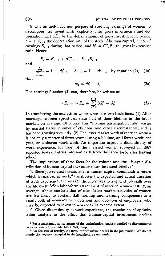
It will be useful for our purpose of studying earnings of women todecompose net investments explicitly into gross investments and de-preciation. Let be the dollar amount of gross investment in period

— 1, the depreciation rate of the stock of human capital, hence ofearnings during that period, and k' = the gross investmentratio. Hence

= E,_1 + —

and

= 1 + rk'_1 — = 1 + by equation (2), (la)

thus

rk5 = — ö:. (2a)

The earnings function (3) can, therefore, be written as

in E1 in E0 + — ö1). (3a)

In transferring the analysis to women, we face two basic facts: (1) Aftermarriage, women spend less than half of their lifetime in the labormarket, on average. Of course, this "lifetime participation rate" variesby marital status, number of children, and other circumstances, and ithas been growing secularly. (2) The lesser market work of married womenis not only a matter of fewer years during a lifetime, and fewer weeks peryear, or a shorter work week. An important aspect is discontinuity ofwork experience, for most of the married women surveyed in 1967reported several entries into and exits from the labor force after leavingschool.

The implications of these facts for the volume and the life-cycle dis-tribution of human-capital investments can be stated briefly

1. Since job-related investment in human capital commands a returnwhich is received at work,6 the shorter the expected and actual durationof work experience, the weaker the incentives to augment job skills overthe life cycle. With labor-force attachment of married women lasting, onaverage, about one-half that of men, labor-market activities of womenare less likely to contain skill training and learning components as aresult both of women's own decisions and decisions of employers, whomay be expected to invest in worker skills to some extent.

2. Given discontinuity of work experience, the conclusion of optimiz-ation analysis to the effect that human-capital investments decline

'For a mathematical statement of the optimization analysis applied to discontinuouswork experience, see Polachek (1973, chap. 3).

6 For the sake of brevity, the term "work" refers to work in the job market. We do notimply that women occupied in the household do not work.

AGE

PRopotenoN WORKING (%)SIZEIn 1966 After First Child Ever

30-34S<S=S>

121212

43464340

64716359

82758488

925294446185

35—39S<S=5>

121212

47454947

67666867

87828892

945336422187

40—44S<5=5>

121212

53525451

70727068

88789193

1,078465446167

Souace.—NLS, 1967 survey.NOTE—S = years of schooling.

continuously over the successive years of life after leaving school is nolonger valid. Even a continuous decline over the years spent in the jobmarket cannot be hypothesized if several intervals of work experiencerather than one stretch represent the norm.

3. The more continuous the participation, the larger the investmentson initial job experience relative to those in later jobs.

Women without children and without husbands may be expected toengage in continuous job experience. But labor-force participation ofmarried women, especially of mothers, varies over the life cycle, dependingon the demands on their time in the household as well as on their skillsand preferences relative to those of other family members. The averagepattern of labor-force experience is apparent in tables 1—3, which arebased on the NLS data reported by women who were 30—44 years of ageat the time of the survey. According to the data:

1. Though less than 50 percent of the mothers worked in 1966, close to90 percent worked sometime after they left school, and two-thirdsreturned to the labor market after the birth of the first child (table 1).Lifetime labor-force participation of women without children or withouthusbands is, of course, greater.

2. Never-married women spent 90 percent of their years after they leftschool in the labor market, while married women with children spentless than 50 percent of their time in it. In each age group, childless women,those with children but without husbands (widowed, divorced, orseparated), and those who married more than once spent less time in themarket than never-married women, but more than mothers marriedonce, spouse present (table 2).

EARNINGS OF WOMEN S8iI'

TABLE 1LABOR-FORCE PARTICIPATION OF Mons: PROPORTION WORKING,

WHITE MARSUED WosszN wrni SPOUSE PRESENT

Ift

-J

Whi

te, w

ith c

hild

ren:

Mar

ried

once

, spo

use

pres

ent

0.57

3.55

6.71

1.14

1.22

1.69

Rem

arrie

d, sp

ouse

pre

sent

...

0.54

2.43

7.85

2.60

2.02

2.00

Wid

owed

1.11

4.25

9.37

1.51

1.44

2.56

Div

orce

d0.

942.

966.

544.

242.

382.

92Se

para

ted

0.74

3.97

7.81

2.71

1.14

2.08

Whi

te, c

hild

less

:on

ce, s

pous

e pr

esen

t1.

015.

18N

ever

mar

ried

...7.

08

Bla

ck, w

ith c

hild

ren:

Mar

ried

once

, spo

use

pres

ent

1.12

3.00

7.12

2.95

Rem

arrie

d, sp

ouse

pre

sent

...0,

962.

447.

434.

93W

idow

ed a

nd d

ivor

ced

1.19

2.23

7.67

4.36

Sepa

rate

d1.

282.

866.

2453

7B

lack

, chi

ldle

ss:

Mar

ried

once

, spo

use

pres

ent

2.33

4.75

Nev

er m

arrie

d...

7.15

TAB

LE 2

WO

RK

HIS

TOR

IES

op W

OM

EN A

GED

30—

44 B

Y M

AR

ITA

L ST

ATU

S (A

VER

AG

E N

UM

BER

OF

YR

AIts

)

VA

PIA

BLE

SAM

PLE

GR

OU

Pe2

h3e3

SSI

zE

6.4

10.4

7.1

10.3

8.4

11.9

10.1

9.8

8.7

9.6

4.39

3.35 1.46

11.8

3.16

2,39

810

.63.

2834

112

.02.

4445

10.8

2.98

133

10.1

2.86

65

4.90

14.5

7.48

14.5

3.3

11.7

1.5

12.9

2.14

3.26

2.05

3.36

1.90

3.68

2.38

2.81

147

153

10.3

11.7

10.8 9.8

3.83

4.58

4.77

4.74

6.45

9.1

10.7

10.3

11.2

13.4

13.6

10.0

4.59

9.6

4.22

9.8

4.20

9.4

4.22

NO

TE—

h1 =

year

s no

t wor

ked

betw

een

scho

ol a

nd fi

rst m

arria

ge; e

1 =

yea

rs w

orke

d be

twee

n sc

hool

and

first

mar

riage

(for

nev

er-m

arrie

d,, =

yea

rs w

orke

d pr

ior

to C

urre

nt jo

b);

h2 =

inte

rval

of n

onpa

rtic

ipat

ion

follo

win

g bi

rth

of fi

rst c

hild

; Cl =

yea

rs w

orke

d af

ter

h2 p

rior

to C

urre

nt jo

b; h

3 =

inte

rval

of n

onpa

rtic

ipat

ion

just

prio

r to

cur

rent

job;

e3

=ye

ars

on c

urre

nt jo

b; L

e =

yea

rs w

orke

d si

nce

scho

ol; £

h =

yea

rs o

f non

part

icip

atio

n si

nce

scho

ol; S

= y

ears

of s

choo

ling;

no. o

f chi

ldre

n.

563

170

149

191

6.9

10.9

4.7

10.9

71 47


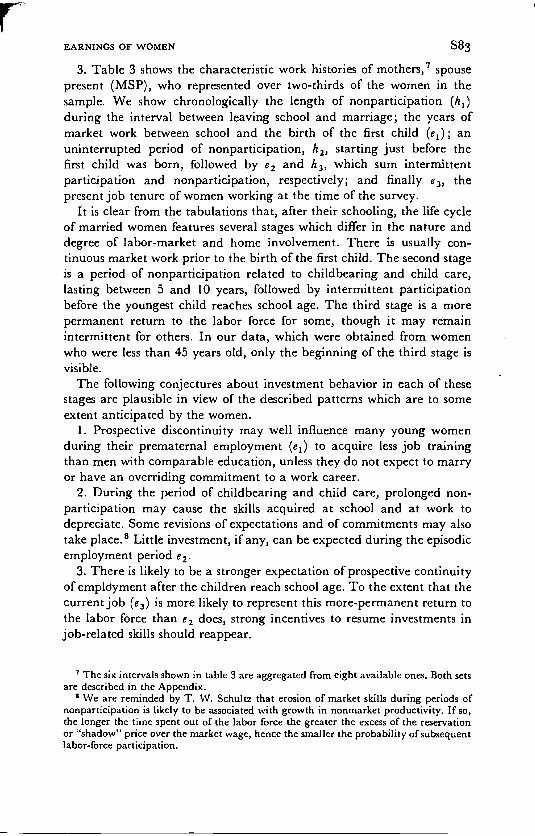
3. Table 3 shows the characteristic work histories of mothers,7 spousepresent (MSP), who represented over two-thirds of the women in thesample. We show chronologically the length of nonparticipation (h1)during the interval between leaving school and marriage; the years ofmarket work between school and the birth of the first child (e1); anuninterrupted period of nonparticipation, h2, starting just before thefirst child was born, followed by e2 and h3, which sum intermittentparticipation and nonparticipation, respectively; and finally e3, thepresent job tenure of women working at the time of the survey.

It is clear from the tabulations that, after their schooling, the life cycleof married women features several stages which differ in the nature anddegree of labor-market and home involvement. There is usually con-tinuous market work prior to the birth of the first child. The second stageis a period of nonparticipation related to childbearing and child care,lasting between 5 and 10 years, followed by intermittent participationbefore the youngest child reaches school age. The third stage is a morepermanent return to the labor force for some, though it may remainintermittent for others. In our data, which were obtained from womenwho were less than 45 years old, only the beginning of the third stage isvisible.

The following conjectures about investment behavior in each of thesestages are plausible in view of the described patterns which are to someextent anticipated by the women.

1. Prospective discontinuity may well influence many young womenduring their prematernal employment (e1) to acquire less job trainingthan men with comparable education, unless they do not expect to marryor have an overriding commitment to a work career.

2. During the period of childbearing and child care, prolonged non-participation may cause the skills acquired at school and at work todepreciate. Some revisions of expectations and of commitments may alsotake place.8 Little investment, if any, can be expected during the episodicemployment period e2.

3. There is likely to be a stronger expectation of prospective continuityof empldyment after the children reach school age. To the extent that thecurrent job (e3) is more likely to represent this more-permanent return tothe labor force than e2 does, strong incentives to resume investments injob-related skills should reappear.

' The six intervals shown in table 3 are aggregated from eight available ones. Both setsare described in the Appendix.

8 We are reminded by T. W. Schultz that erosion of market skills during periods ofnonparticipation is likely to be associated with growth in nonmarket productivity. If so,the longer the time spent out of the labor force the greater the excess of the reservationor "shadow" price over the market wage, hence the smaller the probability of subsequentlabor-force participation.

30—

34:

Wor

ked

in 1

966:

S< 1

21.

93S

=12

—15

0.90

S� 1

60.

37D

id n

ot w

ork

in 1

966,

but

wor

ked

sinc

eS<

12

1.67

s=

12—

150.

81S�

160.

50H

as n

ot w

orke

d si

nce

birth

of f

irst c

hild

:5<

124.

54S

=12

—15

2.28

S� 1

61.

95

35—

39:

Wor

ked

in 1

966:

S< 1

21.

94S

=12

—15

0.98

S�16

1.01

Did

not

wor

k in

196

6, b

ut w

orke

d si

nce

5<12

2.15

S =

12—

151.

20S�

160.

38H

as n

ot w

orke

d si

nce

birth

of f

irst c

hild

:S<

12

4.23

S =

12—

152.

97S�

161.

88

2.37

5.80

2.84

5.41

2.57

2.65

birth

of f

irst c

hild

:2.

236.

292.

904.

651.

853.

57

1.42

9.64

3.21

7.93

1.11

7.20

birth

of f

irst c

hild

:2.

969.

003.

747.

425.

756.

50

3.54

13.5

33.

8511

.62

2.65

10.1

5

3.54

13.0

53.

504.

1310

.21

3.49

3.56

7.64

3.00

4.76

17.5

53.

704.

9214

.56

3.51

6.90

9.50

2.87

TAB

LE 3

Wol

eK H

ISTO

RIE

S O

F M

AR

RIE

D W

OM

EN B

Y A

GE,

ED

UC

ATI

ON

,

VA

RIA

BLE

AG

E A

ND

CA

TEG

OR

Yh1

e1e2

e3X

eSA

MPL

EN

,,SI

ZE

AN

D C

UR

REN

T W

OR

K S

TATU

S

3.18

2.20

1.90

7.45

9.93

3.42

2.21

1.39

2.31

7.36

7.70

2.89

2.22

1.22

2.00

6.79

4.24

2.39

1.31

5.09

1.23

4.75

1.71

3.57

1.42

14.1

8.3.

243.

2110

.21

3.03

1.11

9.15

3.14

2.78

7.98

3.47

2.78

3.40

9.65

12.7

03.

373.

426.

853.

092.

013.

7010

.21

9.84

2.99

2.95

4.72

2.04

1.25

5.46

10.4

56.

982.

72

1.80

6.40

1.18

5.94

1.15

2.62

135

233 35 68 93 14 85 211 34 152

250 43 65 101 8

113

170 26

3.54

17.7

63.

583.

8514

.59

3.16

2.65

12.0

33.

50

I -4

r

TA

BLE

3 (C

ontin

ued)

Cl)

40—

44:

Wor

ked

in 1

966:

S <

122.

413.

2910

.38

S =

12—

151.

554.

168.

74S

� 16

0.93

3.20

6.89

3.94

3.57 3.06

2.95

2.63

1.86

4.93

4.43 4.89

12.1

612

.16

11.1

5

15.7

412

.92

9.68

3.18

2.72

3.65

240

297 29

Did

not

wor

k in

196

6, b

ut w

orke

d si

nce

birth

of f

irst c

hild

:S

< 12

2.35

3.31

12.9

5S

=12

—15

1.39

3.68

10.4

3S

163.

191.

199.

80

1.51

1.24

1.34

6.89

8.23

4.80

... ... ...

4.82

4.92

2.53

22.1

920

.05

17.7

9

3.41

3.36

3.59

89 825

Has

not

wor

ked

sinc

e bi

rth o

f firs

t chi

ld:

S <

126.

232.

6317

.66

S =

12—

153.

364.

8815

.12

S16

3.03

2.67

13.3

5

... ... ...

... ... ...... ... ...

2.63

4.88

2.67

23.8

918

.48

16.3

8

3.93

3.12

2.96

130

141 31

NO

TE—

See

note

s to

tabl

e 2

for e

xpla

natio

n of

var

iabl

es.


These conjectures imply that the investment profile of married womenis not monotonic. There is a gap which is likely to show negative values(net depreciation) during the childbearing period and two peaks beforeand after. The levels of these peaks are likely to be correlated for the samewoman, and their comparative size is likely to depend on the degree ofcontinuity of work experience. The whole profile can be visualized incomparison with the investment profiles of men and of single women.For never-married women, stage 1 (e1) extends over their whole workinglife, and the investment profile declines as it does for men. To the extent,however, that expectation of marriage and of childbearing are strongerat younger ages and diminish with age, investment of never-marriedwomen is likely to be initially lower than that of men. At the same time,given lesser expectations of marriage on the part of the never-married, theirinitial on-the-job investments exceed those of the women who eventuallymarry, while the profile of the latter shows two peaks.

The implications for comparative-earnings profiles are clear: Greaterinvestment ratios imply a steeper growth of earnings, while declininginvestment profiles imply concavity of earnings profiles. Hence, earningsprofiles of men are steepest and concave, those of childless women less so,and those of mothers are double peaked with least overall growth.

III. Women's Wage EquationTo adapt the earnings function to persons with intermittent workexperience we break up the postschool investment term in equation (6)into successive segments of participation and nonparticipation as theyoccur chronologically. In the general case with n segments we may expressthe investment ratio = aj + b1t, i = 1, 2, . . ., n, and

In = In + rs + r + bet) dt. (7)

Here is the initial investment ratio, b is the rate of change of the invest-ment ratio during the ith segment:

1— = = duration of the

ith segment. Note that in (7) the initial investment ratio refers to itsprojected value at t1 = 0, the start of working life. In a work interval mwhich occurs in later life there is likely to be less investment than in anearlier interval j, though more than would be observed ifj continued atits gradient through the years covered by m. In this case, am in equation(7) will exceed

Alternatively, and am can be compared directly in the formulation

in = in E0 + rs + r (a, + b,t) di, (8)

since aj is the investment ratio at the beginning of the particular segment i.

1


While the rate of change in investment is likely to be negative inlonger intervals, it may not be significant in shorter ones. Since thesegments we observe in the histories of women before age 45 are relativelyshort, a simplified scheme is to assume a constant rate of net investmentthroughout a given segment, though differing among segments. Theearnings function simplifies to

in Er = in E0 + rs + r (9)

Whereas (ra1) > 0 denotes positive net investment (ratios), (ra1) < 0represents net depreciation rates, likely in periods of nonparticipation.

The question whether the annual investment or depreciation rates varywith the length of the interval is ultimately an empirical one. Even ifeach woman were to invest diminishing amounts over a segment of workexperience, those women who stay longer in the labor market are likely toinvest more per unit of time, so that aj is likely to be a positive functionof the length of the interval in the cross section.

Thus, even if = a given woman j, if = + f3,tacross women, on substitution, the coefficient b of t may become negligibleor even positive in the cross section. On integrating, and using threesegments of working life as an example, earnings functions (7), (8), and(9) become:

in = a0 + rs + r[a1t1 + + a2(12 — t1)

+ - + a3(t - t2) + - ti)], (a)

in E, = a0 + rs + r(a1e1 + + a2e2(8a)

+ + a3e3 +ln E, = a0 + rs + r(a1e1 + a2e2 + a3e3). (9a)

In this example, is within the last (third) segment, and the middlesegment, e2 = h, is a period of nonparticipation or "home time." Thesigns of b1 are ambiguous in the cross section, as already indicated;the coefficients of e1 and of e3 are expected to be positive, but those ofe2 (or h) negative, most clearly in (9a).

The equations for observed earnings (in differ from the equationsshown above by a term ln (1 — was shown in the comparison ofequations (3) and (4). With k, relatively small, only the intercept a0 isaffected, so the same form holds for in Y, as for in E,.

It will help our understanding of the estimates of depreciation rates toexpress earnings function (9a) in terms of gross-investment rates anddepreciation rates:

in = In E0 + — 6,)

= ln E0 + (rs — 6,) + (r14 — ö,)e1 (9b)+ — + — 63)e3.


This formulation suggests that depreciation of earning power may occurnot only in periods of nonparticipation (h), but at other times as well. Onthe other hand, market-oriented investment, such as informal study andjob search, may take place during home time, so that k > 0. Positivecoefficients of e1 and e3 would reflect positive net investment, while anegative coefficient of h is an estimate of net depreciation. If > 0, theabsolute value of the depreciation rate C5h is underestimated.

IV. Empirical FindingsTables 4—8 show results of regression analyses which apply our earningsfunction to analyze wage rates of women who worked in 1966, the yearpreceding the survey. The general specification is in w = f(S, e, h, x) + u,where w is the hourly wage rate; S is the years of schooling; e is a vectorof work-experience segments; h is a vector of home-time segments andx is a vector of other variables, such as indexes of job training, mobility,health, number of children, and current weeks and hours of work; u isthe statistical residual.

The findings described here are based on ordinary least-squares (OLS)regressions. The tables show shorter and longer lists of variables withoutcovering all the intermediate lists. In view of a plausible simultaneityproblem we attempted also a two-stage least-squares (2SLS) estimationprocedure, which we describe in the next section. Since the 2SLS estimatesdo not appear to contradict the findings based on OLS, we describe themfirst below.

1. Work History Detail and Equation Form

When life histories are segmented into five intervals (eight is the maximumpossible in the data), three of which are periods of work experience andtwo of nonmarket activity,9 both nonlinear formulations (equation forms[7] and [8]) are less informative than the linear specification (9). Ratesof change in investment (coefficient b) are probably not substantial withina short interval, and the intercorrelation of the linear and quadraticterms hinders the estimation. Dropping the square terms reduces theexplanatory power of the regression slightly but increases the visibilityof the life-cycle investment profile. Conversely, when the segments areaggregated, the quadratic term becomes negative but does not quiteacquire statistical significance by conventional standards. The quadraticterm for current work experience is negative and significant. In the case

Tables 2 and 3 show six intervals, including a very short nonparticipation interval h1between school and marriage. This interval is aggregated in other home time in theregressions.

A


of never-married women, one segment of work experience usually coversmost of the potential working life. Here the nonlinear formulation overthe interval is as natural and informative as it is for men.

2. Investment Rates

Table 4 compares earnings functions of women by marital status andpresence of children, tables 5 and table 7 bylifetime work experience. In each table we can compare groups of womenwith differential labor-force attachment. According to human-capitaltheory, higher investment levels should be observed in groups withstronger labor-force attachment.

We can infer these differences in investment by looking at the co-efficients of experience segments, 8j (prematernal), e2 (intermittent, afterthe first child), and e3 (current). These increase systematically frommarried women with children to married women without children tosingle women in table 4, and from women who worked less than half tothose who worked more than half of their lifetime in table 7. An exceptionis the coefficient of e3 which appears to be somewhat higher for the groupwho worked less (see table 7). Note, however, that these coefficients areinvestment ratios (to gross wage rates), not dollar volumes. Since wagerates are higher in the groups with more work experience, the conclusionsabout increasing investment hold for dollar magnitudes, a fortiori, andthe anomaly in table 7 disappears.'°

Classifications by schooling show mixed results. In table 5, whereschooling is stratified by <12, 12—15, and 16+, investment ratios (co-efficients of eg) are lower at higher levels of schooling (with the exceptionof the coefficient of e,). Translated into dollar terms,'1 no clear patternemerges. At the same time in table 6, where the schooling strata are �8,9—12, and 13+, a positive relation between investment volumes andlevels of schooling is somewhat better indicated. Note that the samplesize for the highest-schooling groups (10+) is quite small in table 5,as is that for the lowest-schooling groups (� 8) in table 6.

3. Investment Profiles

Another implication of the human-capital theory refers to the shape ofthe investment profile: it is monotonically declining in groups withcontinuous participation, hence earnings are parabolic in aggregated

10 The coefficient of e3, calculated as a in W/ae, is 15 percent higher in the right-handgroup. However, the wage rate of this group is about 25 percent lower.

Wage rates are roughly 30 percent higher in successive schooling groups.

A

TAB

LE 4

EAR

NIN

GS

FUN

CTI

ON

S, W

HIm

WO

MEN

0

WIT

HC

HIL

DR

ENN

o C

HIL

DR

EN

b£

(4)

NEV

ER M

AR

RIE

D

b(5

)V

ar.

b(1

)I

Var

.b

(2)

tV

ar.

6(3

)1

C ..

......

.S (A

-S-6

) ....

(4-S

-6)2

...2

R

.38

.076

.014

—.0

01

.16

11.5 3.8

—4.

2

..

C S e e2 /i h2 R2

.21

.063

.012

—.0

002

.021

—.0

008

—.0

07.0

00

.25

... 10.5 1.6

—0.

52.

8—

1.9

—1.

50.

2

•..

C S e1 e2 e3 h2 etr

ect

hit bc In H

r....

in W

k ...

N

.09

.064

.008

.001

.012

—.0

12—

.003

.000

2.0

10—

.000

3.0

01.0

44—

.11

.03

—.0

08

... 12.0 2.8

0.3

2.7

—2.

5—

0.7

1.5

3.2

—1.

31.

22.

7—

3.7

1.6

—1.

0

—.4

2.0

81.0

14.0

11.0

15

.002 .006

—.0

21—

.15

.25 ...

... 4.4

1.6

1.3

2.2

—1.

50.

72.

4—

1.2

—1.

31.

7—

0.4

—1.

62.

2...

.55

.077

.026

*—

.000

7t.0

09 ... .000

3—

.011

—.0

008

—.0

12—

.02

—.4

3.2

1 ...

... 4.9

1.5

—1.

11.

5—

0.6

... 1.7

—1.

8—

1.2

—2.

2—

0.3

—4.

4 1.4

....2

899

3... ...

.39

147

... ....4

113

8... ...

NO

TE—

Var

. =va

riabl

e;C

=in

terc

ept;

S =

year

sof

scho

olin

g; A

=ag

e;e

tota

l yea

rs o

f wor

k; e

j =ye

ars

of w

ork

befo

re fi

rst c

hild

; €2

=ye

ars

of w

ork

afte

r firs

t chi

ld;

=cu

rren

t job

tenu

re; h

=to

tal h

ome

time;

h, =

hom

etim

e af

ter f

irst c

hild

; h2

=ot

her

hom

e tim

e; a

r =ex

perie

nce

x tra

inin

g (m

onth

s); e

a=

exp

erie

nce

x ce

rtific

ate

(dum

my)

;hi

t =du

ratio

nof

illn

ess (

mon

ths)

; yes

=ye

ars

of re

side

nce

in c

ount

y; ic

e =

size

of p

lace

of r

esid

ence

at a

ge 1

5; In

Hrs

=(lo

gof

) hou

rs o

f wor

k pe

r wee

k O

tt C

urre

nt jo

b; In

Wks

(log

ofw

eeks

per

yea

r on

curr

ent j

ob;

=no

.of

chi

ldre

n; b

regr

essi

on c

oeff

icie

nt;

=t-r

atio

;R

2co

effic

ient

of d

eter

min

atio

n; N

=sa

mpl

esi

ze.

*T

otal

wor

k ex

perie

nce,

e.

tel. To

tal h

ome

time,

h.

p

—

TAB

LE 5

EAR

NIN

GS

FUN

CTI

ON

S O

F W

MSP

, BY

ScH

oolIN

G

S <

12S

=12

—15

VA

R.

bb

tIs

tIs

t

S =

16+

Isb

t

C S e2 t3C

IDh1 et

red hi

tre

sbc ln

Hrs

in W

itsN

5

R2 N

—.9

84.

7.0

393.

83.

1.0

152.

22.

8.0

121.

84.

7.0

193.

2—

0.6

.001

0.2

0.5

.003

0.5

.000

41.

2.0

162.

4—

.000

6—

1.7

.001

0.5

.06

2.4

—.0

44—

0.9

.045

1.5

—.0

04—

0.4

.17

....2

243

5

—.6

1...

—.0

3.1

055.

1.0

864.

0.0

121.

7.0

081.

3.0

061.

20

0.0

153.

7.0

111.

9—

.013

—3.

4—

.018

—2.

8—

.001

—0.

2—

.006

—1.

0.0

004

2.0

.008

1.9

00

.002

1.3

.036

1.6

—.1

1—

3.9

.031

1.2

—.0

02—

0.2

.14

....1

862

2

.86

....3

6.0

380.

4.1

071.

1.0

231.

5.0

100.

5—

.013

—2.

3—

.016

—3.

0.0

021.

6.0

042.

4—

.023

—2.

2—

.012

—1.

7.0

060.

4.0

021.

0.0

007

0.5

.032

2.1

00

.008

1.2

.05

0.8

—.1

6—

3.4

.05

0.7

—.0

5—

1.5

.16

....3

983

Nom

.—W

MSP

=w

hite

mar

ried

wom

en, s

pous

e pr

esen

t.Se

e ta

ble

4fo

rke

y to

sym

bols

.

— .0

95.0

46.0

16.0

14.0

21—

.002

.002

TAB

LE 6

EAR

NIN

GS

FUN

CTI

ON

S O

F W

MSP

(wim

CH

ILD

REN

), B

Y S

cHoo

LIN

G

I

S�8

S=9—

12S=

13i-

VA

R.

6t

6b

t6

tb

t6

t

R2 N

182

.051

3.2

.055

3.4

.013

1.7

.012

1.5

.009

1.6

.003

0.6

.013

0.7

.009

0.5

—.0

14—

1.8

—.0

10—

1.6

—.0

02—

0.4

—.0

02—

0.4

—.0

011

—2.

3—

.090

—1.

8.0

601.

6—

.019

—0.

4

.21

....2

659

3

.068

2.8

.079

2.7

.021

1.4

.018

1.2

—.0

20—

1.5

—.0

20—

1.4

.009

2.0

.011

2.2

—.0

43—

3.1

—.0

31—

2.8

—.0

05.—

0.4

—.0

04—

0.3

—.0

09—

0.6

—.1

30—

1.1

.090

1.2

—.0

10—

2.0

.27

....3

321

8

=w

hite

mar

ried

wom

en, s

pous

e pr

esen

t. Se

e ta

ble

4 fo

r key

to sy

mbo

ls.

— —

—m

——

— —

— —

-I

•—

,-

U-

—

S.0

491.

6.0

441.

30.

4—

.002

—0.

4e2

—.0

04—

2.1

—.0

28—

1.8

.002

—0.

3—

.008

—0.

5P3

h1—

.011

—1.

5—

.007

—1.

2h2

—.0

06—

0.4

—.0

03—

0.2

his

......

— .0

007

—0.

7ln

Hrs

......

—.0

50—

0.7

mW

/cs

......

—.0

70—

0.6

......

— .0

08—

0.2

.26

....3

2


TABLE 7I

EARNINGS FUNCTIONS OP WMSP BY Wosuc EXPERIENCE

VAR.

Woascan Mosuc THANHALF OF YEARS

Woltxar LESS THANHALF OF YEARS

b t M b t M

C —.28 ... ... —.10 ... .,.S .073 9.4 11.8 .059 7.9 11.0

.009 2.1 4.9.006 1.4 5.6

.003 0.4—.005 —0.6

2.21.5

.017 2.0 4.9—.0002 —0.7 ...—.014 —2.3 2.2

.022 3.8—.001 —1.5—.010 —2.6

1.6...10.7

.011 1.7 2.1 —.004 —0.9 4.7hi: — .0008 —2.1 10.8 — .0001 —0.3 13.7res .002 1.1 12.1° .002 1.0 11.8bc .064 2.8 0.97 .024 1.0 0.90in Hrs — .08 —2.0 3.52 — .13 —4.4 3.40In Wks .07 1.9 3.71 .023 1.0 3.29

R2

—.015 —1.4 2.21 —.001 —0.2 3.18

.22 ... ... .21 ... ...N 536 ... ... 604 ... ...

Nom.—WMSP = white married women, spouse present. See tab! e 4 for key to symbols.

I

experience for men and never-married women.12 In the groups withdiscontinuous participation, the profiles are not expected to be monotonic.

We can summarize the implicit profiles schematically, in terms of thecoefficients of e1, length of work experience before the first child, h1,uninterrupted nonparticipation after the first child, and e3, the currentwork interval. We find (table 4, col. 3) that white married women withchildren (with spouse present) have current investment (ratio whichexceeds the investment (ratio) incurred in experience before the firstchild.13 Presumably, current participation in the labor force, whichtakes place when most of the children have reached school age, is expectedto last longer than the previous periods of work experience. This iscertainly true of women over age 35, and it holds in regressions with orwithout standardization for age.

Looking at regressions within three education levels (tables 5—6), wefind that coefficient of prematernal experience (e1) exceeds the coefficientof current work experience (e3) at the highest level of schooling (in theshort equations, though not in the long ones), and the opposite is true atlower levels. For women without children the coefficient of prematernalwork experience equals that of current work experience. The investmentprofile of never-married women has a downward slope. Comparable

2 In the earnings regressions, the quadratic term of aggregated experience is oftennegative, but not significant statistically.

13 All statements about differences in coefficients refer to point estimates. The dif-ferences are mentioned because they are suggestive, though they would not pass stricttests of statistical significance within a given equation.


early segments of their post school job experience contain higher investmentratios—indeed, the fit implies a linear decline of such ratios over the lifecycle. Evidently, women who intend to spend more time in the labor force ainvest more initially. This is true, presumably, even if their plans are later cchanged following marriage and childbearing.

a

4. Depreciation Rates

The coefficient of home time is negative, indicating a net depreciation ofearning power. During the home-time interval (h1), associated withmarriage or the birth of the first child, this net depreciation amounts to,on average, 1.5 percent per year. In table 5 the depreciation rate is small(—0.2 percent) and insignificant for women with less than high schooleducation, larger (— 1.3 percent) for those with 12—15 years of schooling,and largest (—2.3 percent) for those with 16+ years of schooling. Intable 6, the net depreciation rate is — 1.1 percent for women with ele-mentary schooling or less, — 1.4 percent for women with some high school,and —4.3 percent for women with at least some college. Samplingdifferences probably account for the different estimates in the two tables.The depreciation rate also appears higher in the group who worked morethan half the years (table 7).

It would seem that the depreciation rate is higher when the accumulatedstock of human capital is larger. An exception appears in the comparisonof women without children (married and single) with women with chil-dren. The former have a lower depreciation rate. Of course, these womenspend much less time out of market work, and some of this time might bejob-oriented (e.g., job search).

It is useful to return to the formulation (9b) of the earnings functionfor a closer analysis of the depreciation rates: In E1 = in E0 + (rs — +(ncr — ö1)e1 + (n/cr — öh)h + — ö3)e3. Our coefficient of hometime measures the depreciation rate only if market-oriented investmentk is negligible. This is likely to be true for the period of child caring, theperiod defined as h1 in the regression (/a2 in the tabulations).

An interesting question is whether the depreciation rate (oh) duringnonparticipation is different from the depreciation that occurs at work aswell. The question is whether depreciation due to nonuse of the humancapital stock (atrophy?) exceeds the depreciation due to use (strain?) or

• to aging (?). We are inclined to believe that depreciation through nonuse("getting rusty") is by far more important, particularly in groups of therelatively young (below age 45). Moreover, the atrophy aspect suggestthat depreciation due to nonparticipation is strongest for the market-oriented components of human capital acquired on the job, and weakestfor the inborn, initial, or general components of the human-capital stock.If so, a fixed rate of "home-time depreciation" applicable to on-the-job


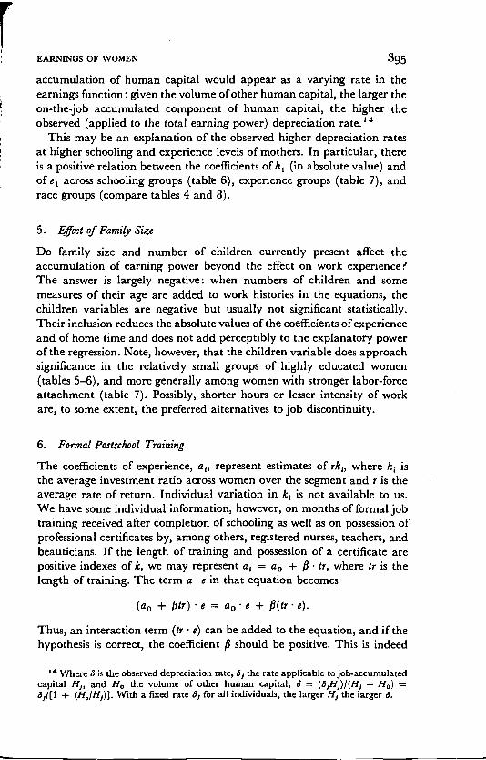
It accumulation of human capital would appear as a varying rate in theearnings function: given the volume of other human capital, the larger theon-the-job accumulated component of human capital, the higher theobserved (applied to the total earning power) depreciation rate.14

This may be an explanation of the observed higher depreciation ratesat higher schooling and experience levels of mothers. In particular, thereis a positive relation between the coefficients of h1 (in absolute value) andof e1 across schooling groups (tabte 6), experience groups (table 7), andrace groups (compare tables 4 and 8).

h

5. Effect of Family

Do family size and number of children currently present affect theaccumulation of earning power beyond the effect on work experience?The answer is largely negative: when numbers of children and somemeasures of their age are added to work histories in the equations, thechildren variables are negative but usually not significant statistically.Their inclusion reduces the absolute values of the coefficients of experienceand of home time and does not add perceptibly to the explanatory powerof the regression. Note, however, that the children variable does approachsignificance in the relatively small groups of highly educated women(tables 5—6), and more generally among women with stronger labor-forceattachment (table 7). Possibly, shorter hours or lesser intensity of workare, to some extent, the preferred alternatives to job discontinuity.

6. Formal Postschool Training

The coefficients of experience, a1, represent estimates of nc1, where k1 isthe average investment ratio across women over the segment and r is theaverage rate of return. Individual variation in k1 is not available to us.We have some individual information, however, on months of formal jobtraining received after completion of schooling as well as on possession ofprofessional certificates by, among others, registered nurses, teachers, andbeauticians. If the length of training and possession of a certificate arepositive indexes of k, we may represent a1 = a0 + In, where In is thelength of training. The term a e in that equation becomes

(a0 + /31r) e = a0 e + fl(tr e).

Thus, an interaction term (In e) can be added to the equation, and if thehypothesis is correct, the coefficient fi should be positive. This is indeed

14 Where ö is the observed depreciation rate, öj the rate applicable to job-accumulatedcapital and H0 the volume of other human capital, ö = + H0) =o,/[1 + With a fixed rate Jj for all individuals, the larger H1 the larger ö.

I

S96 JOURNAL OF POLITICAL ECONOMY EM

the case in most of our equations, confirming the training interpretationof the experience coefficients in the earnings function. Both interactionswith months of job training and with possession of a certificate aresignificant for married women. The training interaction variable is alsopositive in the earnings function of single women, but the certificatevariable is negative. Whereas the negative coefficient of the certification- S.experience variable implies less than average investment behavior amongpersons who work continuously, the corresponding positive coefficient forintermittent workers implies more than average investment behavior.

etred

7. Effects of Mobility hial

Research in mobility has shown that, so long as mobility is not in-voluntary—resulting from layoffs—it is associated with a gain in earnings.However, geographic labor mobility of married women is often exogenous,due to job changes of the husband. In that case, it may militate againstcontinuity of experience and slow the accumulation of earning power. —

We used the information on the length of current residence in a countyor a Standard Metropolitan Statistical Area (SMSA) as an inversemeasure of mobility. This variable has a small positive effect on wage wrates of white MSP women and a significant negative effect for singlewomen. To the extent that mobility is job oriented for single womenand exogenous for married women, the differential signs provide a con- C(

sistent interpretation.0

8. Hours and Weeks in Current Job h

When (logs of) weeks and hours worked in the survey year are included e

in the regression, a negative sign appears for the weekly-hours coefficientand a positive but less significant one for the weeks-worked coefficient. a

The hours' coefficients are smaller for married women than for single twomen and smaller for white than for black women. The negative signof weekly hours may be partly or wholly spurious since some pay periods C

indicated by respondents were weeks or months and the hourly wage ratewas obtained by division through hours. Of course, the direction ofcausality is suspect: it is more likely that women with lower wage rateswork longer hours than the converse. Deletion of the variables, however,has a minimal effect on the equations.

9. Other Variables

Three other variables were included in the equations:1. Twenty percent of the married women who worked in 1966 dropped

out of work in 1967. We used a dummy variable with value 1 if persons I


TABLE 8Epjuur'tos FuNarIONS Os' BLACK Wowzw

10flS

arealsoca teion-.Ongfor

iF'-igs.'us,rister.

rSe

MSP WITH CHILDREN NEVER MARRIED

Var. 1' tVar. I' :

C —.02 ... C —.48 ...S .095 11.2 S .110 3.7

e3hh2etr

.005

.001

.006—.006—.005

.0005

0.80.31.4

—1.2—0.9

1.3

ee2e3Iih2etr

.004—.0003

.001—.02

.001

.0006

0.1—0.2

0.2—.05

1.11.4

ect .008 1.9 ect .003 0.4hit — .0002 —0.5 hIt — .001 — 1.8res .002 0.9 res .001 0.2bc .11 4.0 bc .23 2.7lnHrs —30 —7.4 InHrs —.13 —0.7in Wks .08 2.2 In Wks .03 0.2

.005 0.6 ... ...R2 .39 ... .46 ...N 550 ... N 70 ...

Norc.—MSP white married women, spouse pres ent. See table 4 for key to symbols.

working in 1966 stopped working in 1967, and 0 otherwise.'5 Thisvariable had a negative sign, since it indicated a shorter current jobexperience compared with the prospective work interval of others whocontinued to work in 1967—the completed interval of those dropping outwas not longer than the interval of stayers. In effect, women who droppedout of the labor force in 1967 had wage rates about 5 percent lower thanwomen who continued working, given the same characteristics andhistories.16 The proportion of dropouts is somewhat larger at lowereducation levels.

2. The size of community in which the respondent lived at age 15 hada positive effect on earning power of married women but no effect onthat of single women.

3. Duration of current health problem in months was used as a measureof health levels. It is an imperfect measure for retrospective purposes andshows a very small negative effect on the wage rate.

10. Black Women

The regressions for black MSP (table 8) show experience coefficients abouthalf the size of the corresponding white population. Home time ordepreciation coefficients are not significant; neither are the children

"Not shown in the tables.16 Without standardization, women who had dropped out had wage rates about 10

percent lower than women who continued working.

ige

lleen

itt.IcnIs

e

S

j

S98

variables. The implication is that there is less investment on the job, eventhough black women spent more time than white women in the labormarket. They had more and younger children, on average. The othervariables behave comparably with those in the white regressions exceptthat hours of current work and location at age 15 show stronger effects.In contrast to white women, the size of community of residence at age 15has a positive effect for never-married women as well. Again, the ex-perience coefficients are smaller for black single women than for whites.Perhaps contrary to expectations, neither health problems nor rates ofwithdrawal from the labor force in 1966 differ for black as compared towhite married women with children, spouse present. Rates of return toschooling appear, if anything, to be higher for black women.

V. Lifetime Participation and the Simultaneity ProblemThe earnings function, as we estimate it, relates wages of women toinvestments in schooling and on-the-job training and to a number ofadditional variables already discussed.

The interpretation of some of the independent variables as factorsaffecting earning power may be challenged on the grounds that they mayjust as well be viewed as effects rather than causes of earning power.Presumably, women with greater earning power have stronger jobaspirations and work commitments than other women throughout theirlifetimes. Hence, what we interpret as an earnings function may well beread with causality running in the opposite direction—as a labor-supplyfunction. This argument is most telling for concurrent variables, such aslast year's hours and weeks worked in relation to last year's wage rate.But these variables are of only marginal importance in the wage equationof married women. All other independent variables temporally precedethe dependent variable (current wage rate), which makes the earningsfunction interpretation less vulnerable, though not entirely so for there isa serial correlation between current and past work experience and currentand past earning power. Since lifetime work experience depends, in part,on prior wage levels and expectations, our experience variables are, inpart, determined as well as determining. If so, the residual in our wage equa-tions is correlated with the experience variables, and the estimates ofcoefficients which we interpreted as investment ratios are biased.

How serious this problem is for our analysis depends on the strengthof individual correlations between current and past levels and expec-tations of earning power and on the strength of effect of these prior levelson subsequent work histories of individuals. Of course, when the data aregrouped these correlations and effects are likely to be strong. Better-educated women tend to have higher wage rates than less educatedwomen throughout their working lives, (see, for instance, Fuchs 1967)and as our table 3 shows, they spend a larger fraction of their lives in the

JOURNAL OF POLITICAL ECONOMYEA

lalncCu

thled4

fSt

fi0

r

C

tI


labor force. Table 3 also shows that married mothers who currently donot work, spent, on average, less of their lifetime working than those whocurrently work.

One econometric approach to an estimation of the earnings function inthe presence of endogeneity of "independent" variables is the two-stageleast-squares (2SLS) approach. We estimate work experience as a variabledependent on exogenous variables, some of which are in the earningsfunction and others outside of it. In effect, we estimate a "lifetime labor-supply function." The second step is to replace the work-experiencevariables (e) in the earnings function by the estimated work experience(ê)from the labor-supply function. Parameter estimates in this revisedearnings function are theoretically superior to the original, simple least-squares estimates.'7

Our application of a 2SLS procedure is far from thorough, for tworeasons:

1. It is difficult to implement it on the segmented function, since each:o of the segments would have to be estimated by exogenous variables. For

this purpose we aggregate years of work experience and compare thereestimated earnings function with the original, using aggregated ex-perience.

Y 2. One of the variables in our lifetime labor-supply function is thenumber of children, which is not exogenous. In principle, we shouldexpand the equation system to three to include the earnings function, the

r labor-supply function, and the fertility function. At this exploratory levelwe prefer not to do it, particularly since the fertility function would beestimated by the same variables as the labor-supply function.

The supply function obtained for all white MSP women was

e .514 + .020 SF — .0064 SM — .062

e (5.1) (1.8) (12.0)

where e is total years of work, e, is "potential job experience," that is,years since school, SF is education of wife, SM is education of husband,

and is number of children. The addition of earnings of husbandreduced the coefficient of SM to insignificance without changing thecoefficient of determination, which was R2 = .14.

Estimated values of the numerator (e) are used to reestimate the earn-ings function. A comparison of 2SLS and OLS estimates of the earningsfunction is shown in table 9. If anything, the reestimated function showslarger positive coefficients for (total) experience and stronger negativecoefficients for home time. The children variable becomes even lesssignificant (in terms of 1-values) than before. The reestimation leaves ourconclusions, based on the OLS regressions, largely intact.

Since ê is a function of exogenous variables, it is not correlated with the stochasticterm in the reestimated earnings function.

bor

ler

!pt

15

es.ofto

to

Sioo JOURNAL OF POLITICAL ECONOMY

TABLE 9EARNINGS FUNCtION, WMSP WOMEN, OLS 2SLS

VAR.

OLSft t

2SL

6

S

t

OLS

b t

2SLS

b t

C —.20 ... —.06 ... .19 ... .26 ...S .069 12.8 .063 12.0 .053 9.4 .048 8.5

.010 3.2 .012 2.7 .008 2.8 .010 1.9h1h2e3

—.008.0006.009...

—3.00.23.2

...

—.015— .006

.009...

—7.7—2.3

3.5...

—.007.001.009.005

—1.90.53.42.2

—.013— .006

.010

.006

—5.5— 1.9

3.72.2

cert ... . .. . .. ... .18 5.1 .18 5.1lilt ... ... ... ... —.0003 — 1.3 — .0003 — 1.4res ... ... ... ... .001 1.3 .021 1.4bc ... ... ... ... .044 2.8 .042 2.5lnHrs ... ... ... ... ... —.11 —5.0 —.11 —4.9in Wks... ... ... ... ... .03 1.5 .03 1.6

... .:. ... ... —.010 —1.3 .003 0.3

VU. Earnings Inequality and the Explanatory Power ofEarnings Functions

As table 10 indicates, the earnings function is capable of explaining 25—30percent of the relative (logarithmic) dispersion in wage rates of whitemarried women and about 40 percent of the inequality in the rather smallsample of wage rates of single women in the 30—44 age group who workedin 1966. The earnings function is thus no less useful in understanding thestructure of women's wages than it is in the analysis of wages of males.

58 The (squared) correlation between predicted and actual wage rates was .37. Themean of actual rates was 5.196, with a = .335; the mean of predicted wages W25 5.187,with a = .204.

I

EM

Ma0

Ml

Nvaflcoo

NorE.—WMSP = white married women, spouse present; 5r = months of training; con = certification(dummy); see table 4 for key to other symbols.

VI. PredictionA test of the predictive power of the earnings function was performed on asmall sample of women who did not work in 1966 but were found in thesame first NLS survey to have returned to work in 1967. They were notincluded in our analyses, but their life histories and 1967 wage rates areavailable. The latter were predicted with several variants of the earningsfunction and compared to the reported wage rates. On average, theprediction is quite close, and the mean-square error is even smaller—relative to the variance of the observed wage rates—than the residualvariance in the regressions.' 8 In other words, the predictive poweroutside the data utilized for the regressions is no smaller than within theregressions. The test, however, is weak, because the sample is so small(45 observations). Similar tests will be performed on larger samples ofwomen who return to the labor market in subsequent surveys.

an

diinccindiill

ii

'4aii11

C

C

11

C

I

--

Group c2 (in W) c2 (in Y) u2 (in H) N

Married women byeducation (yrs):<1212—15+16

Total

.17

.18

.17

.21

.17

.16

.81

.92

.77

.76

.78.74

.64

.74

.60

435622

83

.22 .28 .97 .78 .75 1,140

.30

.32.41.30

.62

.43.66.50

.32

.11138

3,230

The dispersion of hours worked during the survey year is much greateramong married women, (in H) = .75, than among men, (In H) =.11. The (relative) dispersion in annual earnings of women is, therefore,dominated by the dispersion of hours worked. This factor is also importantin the inequality of annual earnings of single women and of men ofcomparable ages, but much less so. It is not surprising, therefore, that theinclusion of hours worked in the earnings function raises the coefficient ofdetermination from 28 percent in the hourly-wage equation to 78 percentin the annual-earnings equation of married women, from 41 percent to66 percent for that of single women, and from 32 to 50 percent for that ofmen.

The lesser inequality in the wage-rate structure of working marriedwomen than in the structure of male wages is probably due to lesseraverage, and correspondingly lesser variation in, job investments amongindividuals. At the same time, the huge variation in hours, reflectingintermittency and part-time work as forms of labor-supply adjustments,creates an annual earnings inequality among women which exceeds thatof men. However, the meaning of that inequality, both in a causal andin a welfare sense, must be seen in the family context. As was shownelsewhere (Mincer 1974), the inclusion of female earnings as a componentof family income narrows the relative inequality of family incomes com-pared with that of incomes of male family-earners.

VIII. Some Applications1. The Wage Gap

To compare wage rates of women with wage rates of men, we analyzedearnings of men from the Survey of Economic Opportunity (SEO) forthe same year (1966). We find that the average wage rate of white marriedmen, aged 30—44, was $3.18, compared $2.09 for white marriedwomen and $2.73 for white single women in our NLS data.

EARNINGS OF WOMEN Sio iTABLE 10

EARNINGS INEQUALITY AND EXPLANATORY POWER OP WAGE FUNCTIONS, 1966

595972

I)))

Single womenMarried men

(In W) = variance of (log) wages; g2(In Y) = variance of (log) annual earnings; (In 11) =variance of (log) annual hours of work; RiP,, = coefficient of determination in wage rate function; =coefficient of determination in annual earnings function.

S1o2 JOURNAL OF POLITICAL ECONOMY

TABLE 11EXPERIENCE AND DEPRECIATION COEFFICIENTS, 1966, AGES 30—44

MAIUuF.n

1'

WOMEN

MSINGLE W

b

OMEN

MMARRIED

b

Mat,

M

S .063 11.3 .077 12.5 .071 11.61 .012 9.6 ... ... ... ...

C ... ... .026 15.6 .034 19,4... ... — .0006 258 —.0006 409

C3 .009 3.2 .009 8.0 ... .,.—'.015 6.7 ... ... ... ...—.006 3.5 ... ... ... ...

NLS, 1967; men: SEO, 1967.NOTE—S = years of schooling; h0 = home lime following birth of first child; Ito = other home time;= years of work experience since completion of schooling; = u ent job tenure; 2SLS estimate of

total work experience; It = regression coefficient; M means.

TABLE 12EFFECTS OF WORK EXPERIENCE ON RATES

CoNTRIBUTIOr;': OP

Men'sExperience

(2)

PERCENT OPWAGE GAPEXPLAINED

(3) (4)

ActualExperience

(1)

Married women + .02 + .26 45 42Single women + .32 + .33 7 40Married men + .42 ... ... ...

We inquired to what extent the larger wage ratio (152 percent) ofmarried men to married women and the smaller one (116 percent) ofmarried men to single women can be explained by differences in workhistories and by differences in job investment and depreciation. For thispurpose we estimated a single earnings function of men, aged 30—44, inSEO. The coefficients and means of the variables for these men are shownin table 11, which also gives the NLS estimates for both married andsingle women.

Note that married men and married working women have just aboutthe same average schooling, while never-married women are somewhatbetter educated (by 1 year, on average). The coefficients of schooling aresomewhat lower for married women but higher for single women. Thebig differences are in years of work experience since completion ofschooling. These are 19.4 for men, 15.6 for single women, and 9.6 formarried women. The coefficients of initial experience are .034 for men,.026 for single women, and about half as much for married women.

Multiplying the coefficients by the variables (table 11) and summingyields contributions of postschool investments to the (log of) wage ratesas shown in table 12. These differences, roughly 40 percent betweenhusbands and wives and 10 percent between married men and sirgle

I

L

EARNINGS OF WOMEN S1o3

women, are about 70 percent of the observed difference in wage ratesbetween married men and married women and a half of the differencebetween married men and single women.

If one prefers to be agnostic about the human-capital approach, one6 can treat the earnings function simply as a statistical relation and the

regression coefficients as average "effects" of work experience and ofnonparticipation on wages, without reading magnitudes of investment ordepreciation into them. In that case we may ask how much the sexdifferential in wage rates would narrow if work experience of women wereas long as that of men, but the female coefficients remained as they are.A multiplication of the female coefficients by the male variables in table 11yields the following answers: for married women, 45 percent of the gapwould be erased; for single women, only 7 percent of the much smallergap (table 12, col. 3). The answer is similar for married women if theconverse procedure is used, that is when the work experience of women ismultiplied by the male coefficients (table 12, col. 4). For single women,the reduction of the gap is larger than in the first procedure.

We believe, however, that the weight of the empirical analysis offemale earnings supports the view that the association of lower coefficientswith lesser work experience is not fortuitous: a smaller fraction of time andenergy is devoted to job advancement (training, learning, getting ahead)per unit of time by persons whose work attachment is lower. Hence, the45 percent figure in the explanation of the gap by duration-of-workexperience alone may be viewed as an understatment.

Indeed, comparing the annual earnings of year-round working womenand men in the 30-40 age groups, Suter and Miller found a female-to-male earnings ratio of 46.7 percent. However, the ratio rose to 74 percentfor women in this group who worked all their adult lives. The samecomparison for high school educated persons yielded 40.5 as against74.9 percent. Thus lifelong work experience reduces the wage gap by51 or 58 percent, respectively.19

At this stage of research we cannot conclude that the remaining(unexplained) part of the wage gap is attributable to discrimination, nor,for that matter, that the "explained" part is not affected by discrimin-ation. More precisely, we should distinguish between the concepts ofdirect and indirect effects of discrimination. Direct market discriminationoccurs when different rental prices (wage rates) are paid by employersfor the same unit of human capital owned by different persons (groups).In this sense, the wage-gap residual is an upper limit of the direct effectsof market discrimination. Indirect effects occur in that the existence of

Suter and Miller (1971, table I). Their figures are not quite comparable with ours:their male data come from the Current Population Survey (CPS), and ours from SEO.They compare full-time earnings rather than wage rates, and they compare men andwomen without regard to marital status.

S1o4 JOURNAL OF POLITICAL ECONOMY

market discrimination discourages the degree of market orientation in theexpected allocation of time and diminishes incentives to investment inmarket-oriented human capital. Hence, the lesser job investments andgreater depreciation of female market earning power may to some extentbe affected by expectations of discrimination.

Of course, if division of labor in the family is equated with discrimi-nation, all of the gap is by definition a symptom of discrimination.Otherwise, the analyses of existing wage gaps and of their changes overtime remain meaningful, not tautological.

Our data on work histories show some interesting trends which suggesta prospective narrowing of the wage differential. Table 3 shows that theuninterrupted period of nonparticipation which starts just prior to thebirth of the first child has been shrinking when older women are comparedwith younger ones. Women aged 40—44 who had their first child in the late1940s stayed out of the labor force about 5 years longer than womenaged 30—34 whose first child was born in the late 1950s. Family size isabout the same for both groups, but higher for the middle group (35—39)whose fertility marked the peak of the baby boom. Still, the home-timeinterval in that group is shorter (by about 2 years) than in the oldergroup and longer than in the younger. Thus, the trend in labor-forceparticipation of young mothers was persistent. If, by the time the 30—34-year-old women get to be 40—44 (i.e., in 1977), they will have had 4 yearsof work experience more than the older cohort, and their wage rates willrise by 6 percent on account of lesser depreciation and by another 2—4percent due to longer work experience. Thus, the total observed wagegap between men and women aged 40—44 should narrow by about one-fifth, while the gap due to work experience should be reduced by one-quarter.20

2. The Price of Time and the Opportunity Costs of Children

The loss or reduction of market earnings of mothers due to demands ontheir time in child rearing represents a measure of family investment inthe human capital of their children. This investment cost has beenmeasured by valuing the reduction of market time at the observed wagerate. As pointed out by Michael and Lazear (1971), this valuation isincomplete for two reasons. First, if job investments take place at work,the observed wage rate understates the true foregone wage (gross orcapacity wage) by the amount usually invested during the period when

20 Two opposing biases mar this conjecture: The shorter home-time interval for youngerwomen is an average duration for those who already returned to work. It will lengthenwith the passage of time as additional women return to the labor force. It can be shown,however, that the apparent trend is genuine. At the same time, the assumption of un-changed job-investment behavior leads to an understatement.

-r

'1EARNINGS OF WOMEN S105

earnings are foregone. Second, as is clear from earnings-function analysis,the reduction of market time in turn reduces future wage rates because ofa depreciation in earning power during the period of nonparticipation.The present value of future earnings lost through depreciation is a com-ponent of the opportunity cost of time, hence of children.21

The data and the estimated wage functions permit a tentative, perhapsonly an illustrative, empirical assessment of the opportunity cost ofwomen's time and of children. Specifically, the marginal opportunitycost per hour of a year spent at home—rather than in the market—consists of (1) the gross wage rate (W9), that is the observed but foregonewage (W) augmented by currently foregone investment costs, and (2) thepresent value of the reduction of the future gross wage through currentdepreciation :22

1. We can estimate W9 since W = W9(l — k), and rk is estimated inthe earnings function by a1, the coefficient of work experience (e1)preceding the interruption k = a1/r, where r is the rate of return.

2. The present value of the reduction in W9 due to depreciation, usingr as the discount rate, is d is the (depreciation) coefficientof home time in our wage equations.23

The estimates of marginal opportunity costs of a year (in dollars perhour) are shown in panel I of table 13 for three education groups of whitemothers, aged 35—39. In panel II we calculate total opportunity cx-penditures incurred during the nonparticipation period following thebirth of the first child. This is the period for which the earnings functionsshow significant depreciation coefficients. The length of the period de-pends, in part, on the number of children. Though interpreting all of theforegone earnings this period as an opportunity expenditure on childrenmay be an overstatement, we impose an opposite bias by ignoringsubsequent periods of non participation24 which may also be childinduced. Figures in panel II are the marginal costs per hour (per year)multiplied by h, the duration of home time. Figures in panel III areaverage opportunity expenditures per child (Ne) in each group. Since his in years, the dollar figures in panels II and III should be multipliedby annual hours of work. For example, with 1,500 hours of work per year,the opportunity investment expenditures per child range from about$8,000 spent in 8.8 years by mothers with less than high school educationto $17,000 spent in 5.2 years by mothers with college education or more.

As Robert Willis suggested to us, this is strictly correct for the excess of depreciationduring home time over the depreciation at other times. As we stated earlier, we believethat the Latter is negligible in our age groups.

22 Note that we are looking at household productivity as the return, the purpose ofreducing market work, not as a negative element in costs.

23 A 10 percent discount rate was used in these calculations.24 Inclusion would lead to a 20-25 percent increase in expenditures for the age group.

TAB

LE 1

3M

AR

GIN

AL

PRIc

E O

F TI

ME

AN

D O

PPO

RTU

NIT

Y C

osrs

olt

CH

ILD

REN

, 196

6,W

OR

KIN

G W

rnm

MO

THER

S (A

GED

35—

39)—

BY

OF

SCH

OO

LIN

G($

)

NO

TE..—

hC =

dura

tion

of h

ome

time;

=no

.of

chi

ldre

n.

0

PRIC

E O

FTI

ME

PER

HO

UR

TOTA

L O

PPO

RTU

NIT

YEX

PEN

DIT

UR

ES O

N C

HIL

DR

ENO

PPO

RTU

NIT

Y E

XPE

ND

ITU

RES

PER

CH

ILD

<12

12—

15(I

)16

+<1

212

—15

16+

(II)

<12

12—

15(I

II)

16+

1. O

bser

ved

wag

e2.

Cap

acity

wag

e3.

Dep

reci

atio

nSu

m (2

+ 3

)A

ssum

ing

1,50

0 hr

wor

k pe

r yea

r

1.66

1.96

0.05

2.25

2.59

0.30

3.54

4.60

1.40

14.6

016

.33

18.5

117

.25

18.8

724

.05

0.44

2.18

7.32

4.23

5.00

0.13

5.52

6.41

0.73

6.60

8.57 2.63

2.01

2.89

6.00

17.6

921

.05

31.3

75.

137.

1411

.20

... ... ... ...

... ... ... ...

... ... ... ...

......

...8.

807.

265.

233.

452.

962.

812.

552.

451.

86

7,74

0... ... ...

10,7

10 ... ... ...

16,8

00 ... ... ...

EARNINGS OF WOMEN S1o7

Only panel I represents the marginal price of time. Note that theobserved wage rate25 represents 80 percent of the marginal price of anhour below college levels and only 60 percent at higher levels. The sameproportions hold in the other two panels. However, figures in thesepanels are not prices but expenditures which depend on both the price oftime and the number of children and the average home-time intervalper child. Both of these variables can be viewed as responses to the mar-ginal price of time. As the table indicates, observed wage rates and, evenmore so, marginal prices of time (panel I) increase with education. Lesserfertility and closer spacing of children are the responses :26 both numbersof children and interval of home time per child diminish. Consequently,the differences in total expenditures by education level are reduced. Whilethe marginal price of time of the highest education group is three times ashigh as that of the lowest, the expenditures per child are a little overtwice as high, and total expenditures are only 70 percent higher.

Since the opportunity costs of labor-force withdrawal ("home time")are not quite the same thing as the opportunity costs of children, we againcaution the reader to view the estimates of table 13 as largely illustrative.They clearly illustrate the point which the title of this paper intends toconvey: foregone market-oriented human capital of mothers is a part ofthe price of acquiring human capital in children, and more generally, aprice exacted by family life. Of course, the greater market specialization,longer hours, and greater intensity of work and ofjob training on the partof husbands and fathers can be viewed as a "price exacted by familylife" in exactly the same sense.

Implicitly, families balance such prices against perceptions of receivedbenefits.27 Of course, both perceptions of net benefits and prices change.While perceptions are matters of individual psychology and of culturalclimate, the marginal opportunity cost of time has risen secularly with therise in real wages and with the growth of human capital. It is natural foreconomists to connect to this basic fact both upward trends in labor-forceparticipation of women and downward trends in fertility,28 changes inthe family, and even some of the rhetoric which accompanies thesedevelopments.

25 In principle, wage rates just before the period Ii are required. The wage at ages35—39 represents, on average, a small overstatement: wage profiles of married women withchildren are relatively flat in the age span 25—39 within education groups.

26 Direct evidence on closer spacing at higher levels of education is shown in researchfor a Columbia Ph.D. dissertation by Sue Ross (1973). In the NLS data, there is a strong cor-relation between the length of home time and the birth interval from oldest to youngestchild.

27 Some of these benefits are analyzed in the papers of Lee Benham and ArleenLeibowitz in this volume.

2 B For economic analyses which bear on the upward secular trends in labor-forceparticipation of married women, see Mincer (1962) and Cain (1966). For analysesbearing on fertility trends, see "New Economic Approaches to Fertility," J.P.E., vol.81, no. 2, suppl. (March/April 1973).

Si o8 JOURNAL OF POLITICAL ECONOMY

AppendixNote on the Construction of Work-Experience Intervals

The 1967 NLS survey of women aged 30—44 permits a division of time elapsedsince leaving school into, at most, eight intervals. The following information wasused in constructing these intervals: (a) Dates were available for school leaving(S), first marriage (M), birth of first child (C), start of first job, return to laborforce after birth of first child, start of current job, and end of last job, if currentlynot working. (b) Number of years during which the woman worked at least 6months between: (1) school leaving and first marriage, (2) marriage and birth offirst child, (3) return to labor force after the first child, and (4) the start of currentjob.

On this basis, we describe the intervals in the order of their chronologicalplacement: interval h1 (on average, half a year) is the interval between schooland first job; e1 is the number of years of work between school and marriage. Theplacement and continuity of this interval checks rather closely with the data,though direct statements are absent; e2 is years worked (similarly defined) betweenfirst marriage and birth of first child; h2 is the residual home time, given informa-tion on the length of interval between first marriage and birth of first child. Theassumption of continuity and order of placement of e2 and h2 are somewhatarbitrary. They are justified by evidence of frequent identity of job e1 and e2 andthe plausibility of h2 starting during pregnancy. Indeed, h2 is a fraction of a year,on average; h3 is the uninterrupted interval of home time following the birth ofthe first child. It is placed by direct information; e3 is years of work and h4 theresidual amount of time in the interval between returning to the labor force atthe end of h3 and start of current job. However, neither e3 nor h4 needs to becontinuous. The succession of h4 after e3 is more plausible than the converse. Also(e3 + h4) is, on average, about 3 years altogether; e4 is clearly defined and placedas the current job interval.

In tables 2 and 3 we aggregate (e1 + e2) and call it e1, (h2 + h3) is h2, andthe other intervals are correspondingly renamed.

In the regressions we added h1 to h3 to get h2 other home time. Separately, ortogether, these intervals are quite short and show little effect in our analysis.

4

Comment

Otis Dudley DuncanUniversity of Michigan

For readers, other than economists specializing in studies of humancapital, the most controversial sections of Mincer and Polachek's paperare likely to be the introductory statements of the motivation of the re-search and the authors' calculation which suggests that not less than halfthe wage gap between married women and men is due to sex differencesin length and continuity of work histories.

To their initial rationalization of the division of labor within the familyin terms of "complementarity and substitution relations in the householdproduction process" and "absolute and comparative advantages due todifferential skills and earning powers," the authors quickly add the dis-claimers that sex linkage of intrafamily role differentiation is "subject totechnological and cultural changes" and that such changes along with"discriminatory attitudes. . . in the labor market" are outside the scopeof the study. Most feminists and many sociologists would presumablyrespond that with this much of the problem out of scope, what remains islikely to be misleading.

In technical terms, the issue is whether the "statistical residual" u inthe general specification of the model is indeed uncorrelated with thevector e so that the coefficients of e, (experience segments) in the earningsfunction are unbiased estimates of the investment in human capitalappropriate to the wife's role in the household. Mincer and Polachek doaddress the problem of bias in their somewhat cursory treatment oftwo-stage least-squares estimation of the earnings function. But there theconcern is with possible simultaneity of wage levels and experiencevariables. The more serious question may be whether such institutionaland cultural factors as discrimination and employers' unwillingness toinvest in training female workers—all taken to be beyond the scope of thestudy and presumably captured only in the residual u—act as commoncauses of wage levels and work experience.

Slog

rSt 10 JOURNAL OF POLITICAL ECONOMY

Indeed, in the remarks appended to the calculations on the wage gap,Mincer and Polachek come perilously close to a premature closure oftheir conceptual scheme. Having attributed half the gap to sex differencesin work experience they go on to observe that the lower coefficient for thatexperience among women may also be attributable to lower workattachment on the women's part. But the sex difference in work ex-perience and the sex difference in coefficient for work experience providean exhaustive decomposition of the sex difference in wages, net of initialendowment as of the beginning of the work history. Hence, the paperseems to be saying that women get about what they deserve in the jobmarket.'

Many technical and conceptual improvements are required if thestrategy opened up by this paper is to be productive. Mincer and Polachekseem amply aware of the frailty of their estimates, due to sample sizeand crudity of measurement. The hypercritical reader, however, will notfail to note various places where the authors seemingly read their tables a Blittle too smoothly.

On the conceptual side, much work remains to be done before aserviceable model emerges from this kind of work. Treatment of the"activities, and characteristics of other family members," mentioned at athe outset, is underdeveloped in the present formulation, while the labor- risupply function is admittedly inadequate and a fertility function is lacking. aMore directly to the point of the inquiry at hand, one is disappointed to hfind no effort to include the quality of the work experience, and this isperhaps a more serious omission than the parallel inattention to qualityof schooling. One indication that investigation of this facet of the problemcould be productive is given by table 4.7 in Dual Careers (Parnes, Shea,Spitz, and Zeller 1970, p. 114), wherein it appears that the effect of therate of lifetime labor-force participation on the wage rate is substantiallygreater for white-collar than for blue-collar workers among currentlyemployed women. In this connection Mincer and Polachek do investigatethe interaction of work experience and schooling with respect to wagerate. Close inspection of their tables 5 and 6 turns up some disconcertingvariations in coefficients by years of schooling. At this point errors in thedata and misspecifications of the model are hard to tell apart.

One can surmise that when all the truly endogenous and relevantcauses and effects of the earnings of women are explicitly represented inthe model, it will either be underidentified or else have been broadenedto include the "sociological" exogenous variables ruled out of scope inthis initial and productive foray. In trying to get the model properlyspecified, however, one need not expect too much help from the disciplineof sociology as such, geared as it is to the production of dialectic ratherthan discovery.

The authors' own views on the points at issue are made much clearer in their revision,which was not available when this comment was prepared. H

this pdf is a selection from an out-of-print volume from the … · · 2015-03-04volume...

Documents