thermal performance of buildings with post ... - core
TRANSCRIPT

THERMAL PERFORMANCE OF BUILDINGS WITH POST-TENSIONED TIMBER STRUCTURE
COMPARED WITH CONCRETE AND STEEL ALTERNATIVES
A thesis submitted in partial fulfilment
of the requirements for the Degree
of
Doctor of Philosophy
in
Civil Engineering
In the University of Canterbury
by
Nicolas Perez Fernandez
Department of Civil and Natural Resources Engineering
University of Canterbury
2012

Abstract
i
Abstract
This thesis describes the influence of thermal mass on the space conditioning energy consumption
and indoor comfort conditions of multi-storey buildings with concrete, steel and timber structural
systems. The buildings studied were medium sized educational and commercial buildings. When
calculating a building’s life-cycle energy consumption, the construction materials have a direct
effect on not only the building’s embodied energy but also on the space conditioning energy. The
latter depends, amongst other things, on the thermal characteristics of the building’s materials;
thermal mass can also be an influence on comfort conditions in the building.
A modelling comparison has been undertaken between three very similar medium-sized buildings,
each designed using structural systems made primarily of timber, concrete and steel. The post-
tensioned timber version of the building is a modelled representation of a real three-storey
educational building that has been constructed recently in Nelson, New Zealand. The concrete-
and steel-structured versions have been designed on paper to conform to the required structural
codes and meet, as closely as possible, the same performance, internal space layout and external
façade features as the real timber-structured building. Each of these three structurally-different
buildings has been modelled with two different thermal envelopes (code-compliant and New
Zealand best-practice) using a heating, ventilating and air conditioning (HVAC) system with heating
only (educational scheme) and heating and cooling (commercial scheme). The commercial system
(with cooling) was applied only to the buildings with the best-practice thermal envelope.
The analysis of each of these nine different construction and usage categories includes the
modelling of operational energy use with an emphasis on HVAC energy consumption, and the
assessment of indoor comfort conditions using predicted mean vote (PMV). From an operational
energy use perspective, the modelling comparison between the different cases has shown that,
within each category (code-compliant, low-energy and low-energy-commercial), the principal
structural material has only a small effect on overall performance. The most significant differences
are in the building with the best-practice thermal envelope with the commercial HVAC system,
were the concrete building has slightly lower HVAC energy consumption, being 3 and 4% lower
than in the steel and timber buildings respectively
The assessment of indoor comfort conditions during occupied periods through using PMV for each
of the three categories shows that the timber structure consistently exhibited longer periods in the
over-warm comfort zone, but this was much less pronounced in south-facing spaces. To examine
the reasons for the less acceptable PMV in the timber-structure versions, an analysis of indoor
timber and concrete surface temperatures was carried out in both buildings. It was found that,
particularly in north-facing spaces, there were large diurnal swings in the temperatures of timber

Abstract
ii
surfaces exposed to solar radiation. These swings were much less in the case of concrete surfaces
so the environment was perceived to be more comfortable under such conditions because of the
reduced influence of higher mean radiant temperatures.
To moderate this potential downside of solar-exposed internal timber surfaces, better results are
achieved if, when timber is used for thermal mass, the timber is not exposed to direct solar
radiation, for example locating it in the ceilings or on the south side of the building.
Two other approaches to combating the potential overheating problem in the timber-structured
buildings were analysed in an illustrative mode; addition of external louvres to reduce direct solar
gains at critical times of day and year; and use of phase change material (PCM) linings to act as
light-mass energy buffers. Although external louvres increase comfort conditions significantly by
reducing the periods of an overly warm environment, they produce an increase in heating energy
consumption through reducing beneficial solar gains. The use of PCM linings shows little benefit to
overall indoor comfort conditions for the building of this case-study.

Acknowledgements
iii
Acknowledgments
This research investigation presented in this thesis was carried out at the Department of Civil and
Natural Resources Engineering, University of Canterbury, New Zealand, made possible by
financial support from the Structural Timber Innovation Company (STIC) and the University.
Financial support was also provided by the Chilean National Commission for Scientific and
Technological Research (CONICYT). I highly appreciate these research scholarships provided
during my candidature in this PhD programme.
I would like to express my most sincere gratitude to my senior supervisor, Professor Andrew
Buchanan, Professor of Timber Design, Department of Civil and Natural Resources Engineering,
for his guidance, invaluable advice, patience and continuous encouragement, without which the
research would not have been successful. His excellent ideas helped me to formulate the research
and carry out the work in a smooth way.
I would also like to express my sincere gratitude to my supervisor, Dr Alan Tucker, in the
Department of Mechanical Engineering at the University of Canterbury, for his extensive help,
constant guidance and coherent effort in terms of regular advice and encouragement throughout
this research. In particular, I am deeply indebted to him for providing his outstanding help with
respect to thesis writing, especially, his promptness in returning my drafts. His prudence in
reviewing my writing was superb.
Sincere thanks are also due to Stephen John in his role as Sustainability Researcher at the
Department of Civil and Natural Resources Engineering for helping in all the background work
necessary to make things happen along this research. Special thanks to Dr. Larry Bellamy for his
contribution in the outline of this research.
I want to extend my gratitude to all the people who gave me technical advice and assistance over
the duration of the research: Jonathan Halliday and Simon Taylor from Aurecon, Christopher White
from Schneider Electric, John Wall and Tony Greep from the Nelson Marlborough Institute of
Technology, and Tony Sellin from University of Canterbury’s energy management team.
Finally, thanks to my family-members and friends who have made significant contribution in
supporting my study. Heartfelt thanks goes to my wife Francisca, son Renato and little son
Santiago for their understanding, support and love during every moment of this research work.


Table of Contents
v
Table of Contents:
Abstract ............................................................................................................................................... i
Acknowledgments ............................................................................................................................. iii
Table of Contents: .............................................................................................................................. v
List of Figures: .................................................................................................................................. xi
List of Tables: .................................................................................................................................. xvi
1 Introduction ................................................................................................................................ 1
1.1 Construction materials and operational energy .................................................................. 1
1.2 Case study buildings used for comparison in this research ............................................... 2
1.3 Objectives: .......................................................................................................................... 3
1.4 Thesis outline ..................................................................................................................... 5
2 Background - literature review ................................................................................................... 7
2.1 Environmental impacts of multi-storey buildings ................................................................ 7
2.1.1 Multi-storey concrete and steel buildings’ contribution to sustainable development ... 7
2.1.2 Multi-storey timber buildings - structural systems ....................................................... 9
2.1.2.1 Contribution of timber structures to sustainable development ............................. 9
2.2 Comparison of energy and carbon footprint of buildings built in concrete, steel, or timber ..
.......................................................................................................................................... 10
2.2.1 Ratio of embodied to operational energy, and relative proportion of operational
energy end-uses in total life-cycle energy consumption .......................................................... 11
2.2.2 The aspects of structural systems that influence operational energy consumption of
buildings .................................................................................................................................. 12
2.2.2.1 Energy as the indicator chosen for operational environmental impacts ............. 12
2.3 The focus on thermal mass .............................................................................................. 13
2.3.1 The effect of thermal mass on environmental impacts of domestic buildings ........... 13
2.3.1.1 The influence of thermal mass on operational energy consumption of houses in
New Zealand ........................................................................................................................ 15
2.4 The effect of thermal mass on the energy consumption of multi-storey commercial
buildings ...................................................................................................................................... 16
2.4.1 Influence of thermal mass on cooling energy consumption. ..................................... 17
2.4.2 Influence of thermal mass on heating energy consumption. ..................................... 18
2.5 Thermal mass - parameters affecting the performance .................................................... 19
2.5.1 Appropriate amount of thermal mass ........................................................................ 19
2.5.1.1 Increase of thermal linkage ................................................................................ 20
2.5.2 Thermal mass materials ............................................................................................ 20
2.5.3 Thermal mass location and distribution ..................................................................... 21

Table of Contents
vi
2.6 Summary of thermal mass ................................................................................................ 22
2.6.1 Conclusions from the literature review – What is the gap in existing literature that this
research is going to fill? ........................................................................................................... 23
2.6.1.1 Additional literature ............................................................................................ 24
3 Methodology: Overview and Justification ................................................................................ 25
3.1 Introduction ....................................................................................................................... 25
3.2 Methodology outline: ........................................................................................................ 26
3.3 Merits of modelling vs real buildings ................................................................................. 27
3.4 Choice of case study buildings ......................................................................................... 28
3.5 Variation to the models ..................................................................................................... 28
3.5.1 Addition of cooling capability to extend to commercial applications .......................... 30
3.6 Extension of the Arts building model to other hypothetical buildings ................................ 32
3.7 Operational energy emphasis ........................................................................................... 33
3.8 Validation of models ......................................................................................................... 34
3.8.1 Metering requirements .............................................................................................. 35
3.8.2 Climatic data – Actual vs TMY .................................................................................. 36
3.9 Accuracy of model vs actual comparison, and implications this will have on the validity of
results .......................................................................................................................................... 37
3.9.1 Calibration methods used in literature ....................................................................... 38
3.9.1.1 The influence of schedules only ......................................................................... 39
3.9.1.2 The influence of infiltration only .......................................................................... 40
3.9.2 Temperature differences ........................................................................................... 40
3.9.3 Summary of a benchmark for the accuracy of building models ................................. 41
3.10 Modelling software requirement – Choice of Software ..................................................... 42
3.10.1 Modelling direct solar radiation .................................................................................. 43
3.10.2 Methods for testing whole-building energy simulation programs applied to VE ........ 44
3.11 Interpreting data comparison between building variants (energy, and comfort conditions)
and checking sensitivity of the comparison to the assumptions made ........................................ 46
3.11.1 Modelling of the Test building and its comparison with the Arts building: ................. 47
3.11.1.1 How representative of the Arts building, is the Test building?............................ 48
3.11.1.2 HVAC in the Test building .................................................................................. 49
3.11.2 The responsiveness of VE to the increment of thermal mass in buildings ................ 49
3.11.2.1 Thermal mass in the floor system and the inclusion of shear walls ................... 51
3.11.2.2 The influence of increasing heat transfer coefficient of the massive concrete slab
by reducing surface resistance ............................................................................................ 54
3.11.3 The method of modelling thermal mass of structural frame elements by using stand-
alone walls ............................................................................................................................... 56

Table of Contents
vii
3.11.4 Drawing conclusions from modelling capabilities of VE and the influence of these in
further modelling ...................................................................................................................... 59
4 Modelling of case-study buildings ............................................................................................ 61
4.1 Building model introduction .............................................................................................. 61
4.1.1 Timber structural system in the actual Arts building .................................................. 62
4.1.2 Arts building space layout description ....................................................................... 62
4.1.2.1 Arts building space floor area and external facades description ........................ 64
4.2 Construction of the case study buildings .......................................................................... 65
4.2.1 Construction categories and attributes ...................................................................... 66
4.2.2 Attributes of construction and their disaggregation into materials ............................. 68
4.3 Construction of the Timber-low, Concrete-low, and Steel-low buildings........................... 68
4.3.1 Thermal envelope description ................................................................................... 69
4.4 Structural elements contributing thermal mass ................................................................ 70
4.4.1 Shear walls ................................................................................................................ 71
4.4.2 Structural suspended floors ....................................................................................... 72
4.4.2.1 Modelling of suspended floor systems ............................................................... 73
4.4.3 Modelling of the structural frame ............................................................................... 73
4.4.3.1 Specific volumes of stand-alone-walls ............................................................... 75
4.5 Thermal conditions in the modelling of buildings .............................................................. 78
4.5.1 Software used ........................................................................................................... 78
4.5.2 Location and weather data ........................................................................................ 79
4.5.3 Occupancy and operation (Profiles) .......................................................................... 81
4.5.4 Room thermal templates ........................................................................................... 82
4.5.5 Lighting Data ............................................................................................................. 83
4.5.6 Conditioned and unconditioned thermal zones ......................................................... 84
4.6 Modelling of the HVAC System in the Virtual Environment’s Apache HVAC tool............. 86
4.6.1 Overview of the HVAC system (educational and commercial) .................................. 86
4.6.1.1 Educational HVAC system ................................................................................. 86
4.6.1.2 Commercial HVAC system ................................................................................. 87
4.6.2 Ventilation (mechanical and natural) ......................................................................... 89
4.6.2.1 Night-time ventilation .......................................................................................... 90
4.6.3 Heating and cooling ................................................................................................... 91
4.6.3.1 Heating and cooling in the educational HVAC system ....................................... 91
4.6.3.2 Heating and cooling in the commercial HVAC system ....................................... 92
4.7 Modelling method of the heating and cooling equipment ................................................. 93
4.7.1 AHU heating and cooling coil .................................................................................... 93
4.7.2 Fan-coil unit – computer room ................................................................................... 93

Table of Contents
viii
4.7.3 Hydronic heating and cooling induced air systems ................................................... 94
4.7.4 Hot water Radiators ................................................................................................... 94
4.7.5 Hydronic Heated Slab ............................................................................................... 95
4.7.5.1 Heated slab modelling in the Apache HVAC tool ............................................... 96
4.7.6 Heating and cooling sources ..................................................................................... 97
4.7.6.1 Boilers - heating sources .................................................................................... 97
4.7.6.2 Chillers: .............................................................................................................. 97
5 Calibration of energy modelling ............................................................................................... 99
5.1 The T-Block building ......................................................................................................... 99
5.2 Geometry and construction of T-Bock and comparison with the Arts building ............... 101
5.2.1 Ventilation ................................................................................................................ 103
5.2.2 Comparison of T-Block and Arts building sizes ....................................................... 103
5.2.3 Construction ............................................................................................................ 104
5.3 Thermal conditions in T-Block ........................................................................................ 105
5.3.1 Profiles in the T-Block building ................................................................................ 106
5.3.2 Thermal templates in the T-Block building .............................................................. 106
5.4 Real time Weather File production ................................................................................. 108
5.5 Metering layout and equipment ...................................................................................... 111
5.5.1 Thermal Energy Monitoring ..................................................................................... 111
5.5.2 Electric Energy Monitoring ...................................................................................... 112
5.5.3 Temperature monitoring .......................................................................................... 113
5.6 Monitoring results and comparison with modelled data .................................................. 115
5.6.1 Electric energy consumption comparison ................................................................ 115
5.6.2 Thermal energy consumption comparison .............................................................. 117
5.6.3 Air Temperature comparison in T-Block .................................................................. 118
5.6.4 Indoor air temperature in Level 1, Level 2, and Level 3 .......................................... 120
5.6.4.1 Indoor air temperature in Level 2 - detailed temperature analysis ................... 123
5.6.4.2 Indoor air temperature in Room 2A and 2B in Level 2 - detailed temperature
analysis ......................................................................................................................... 126
6 Assessment of the accuracy of energy modelling in the Arts building ................................... 129
6.1 Introduction ..................................................................................................................... 129
6.2 Brief description of monitoring system in the Arts building ............................................. 129
6.3 Benchmark of the modelled heating energy consumption in the Arts building ............... 131
6.4 Comparison between indoor air temperatures in rooms of the Arts building .................. 134
6.4.1 Arts building - rooms facing south on Level 1: ........................................................ 135
6.4.2 Rooms facing south on Level 2 and Level 3: .......................................................... 136
6.4.3 Gallery’s all levels combined values - air temperature ............................................ 137

Table of Contents
ix
6.5 Summary of the accuracy in the modelling of the Arts building ...................................... 138
7 Results of energy modelling analyses ................................................................................... 140
7.1 Introductory clarifications to results ................................................................................ 140
7.2 Assessment of building’s operational energy performance ............................................ 142
7.2.1 Energy consumption in buildings with the code-compliant thermal envelope ......... 142
7.2.2 Energy consumption in buildings with the best-practice thermal envelope (No
summer operations) ............................................................................................................... 143
7.2.3 Energy consumption in buildings with the best-practice thermal envelope and the
commercial HVAC system (Year-round operations) .............................................................. 144
7.2.4 Assessment of Energy - final discussion ................................................................. 145
8 Assessment of indoor environmental conditions ................................................................... 148
8.1 Rooms selected for PMV assessment ............................................................................ 148
8.1.1 Gallery ..................................................................................................................... 149
8.1.2 Studio 201 ............................................................................................................... 150
8.2 PMV Analysis ................................................................................................................. 151
8.2.1 PMV in the Landing-Gallery space in Level 2 – North façade ................................. 152
8.2.2 PMV in Staff room in Level 2 – North façade .......................................................... 155
8.2.3 PMV in Studio room in Level 2 – South façade ....................................................... 156
8.2.4 Assessment of the Influence of default comfort parameters ................................... 157
8.3 Indoor air and surfaces temperature comparison between the Timber, Concrete and Steel
buildings: ................................................................................................................................... 158
8.3.1 Whole year, weekly averaged temperature: ............................................................ 158
8.3.2 Hourly temperature comparison – The choice of a winter and a summer
representative week ............................................................................................................... 160
8.3.3 Surfaces to be assessed ......................................................................................... 163
8.3.4 Gallery temperature analysis – North facing ........................................................... 164
8.3.4.1 Level 2 Gallery – Detailed temperature analysis .............................................. 164
8.3.4.2 Level 1 and Level 3 Gallery – Air and surfaces temperatures .......................... 167
8.3.5 Studio 201 surface and air temperature analysis – South facing ............................ 169
8.3.5.1 Studio 210 - Shear walls .................................................................................. 169
8.3.5.2 Studio 201 – Floor surface temperature ........................................................... 171
8.4 Discussion of indoor environmental conditions .............................................................. 173
8.4.1 PMV assessment - final discussion ......................................................................... 173
8.4.2 Surface and air temperatures - Discussion ............................................................. 174
9 Improvement of energy performance and comfort conditions ............................................... 176
9.1 Night-time ventilation and solar shading system replacement ....................................... 176
9.1.1 Louvres .................................................................................................................... 176

Table of Contents
x
9.2 Results on energy consumption ..................................................................................... 177
9.3 Results of PMV assessment ........................................................................................... 178
9.3.1 PMV of the Landing-Gallery space – North façade ................................................. 178
9.3.2 PMV in Staff room Level 2 – North façade .............................................................. 179
9.3.3 PMV in Studio room in Level 2 – South façade ....................................................... 181
9.3.4 Discussion on improvement of energy performance and comfort conditions .......... 182
9.4 Improvement of the energy performance and comfort conditions of the Timber building –
use of PCM ................................................................................................................................ 182
9.4.1 PCM materials - Introduction ................................................................................... 182
9.4.1.1 Setup of models in PCM-Express .................................................................... 184
9.4.2 Results of PCM materials analysis: ......................................................................... 185
10 Research conclusions: ....................................................................................................... 188
10.1 Conclusions .................................................................................................................... 188
10.2 Future research .............................................................................................................. 192
References .................................................................................................................................... 194
Appendices: .................................................................................................................................. 201
A. Modelling of the test building and its comparison with the Arts building: ............................... 201
B. Representation of Solar Insolation in VE Apache .................................................................. 203
C. Constructions ......................................................................................................................... 205
D. Thermal templates ................................................................................................................. 209
E. Mechanical Ventilation and heating data ............................................................................... 211
F. THERM analysis of under-floor heated slab conductivity ...................................................... 213
G. Influence of steel purlins on space conditioning energy ..................................................... 215
H. Variable PMV assessment ..................................................................................................... 217
I. PCM analysis ......................................................................................................................... 219
J. Report from PCM-Express ..................................................................................................... 221
K. Simplistic model of heating required for Arts building during August 2011 ............................ 225

List of Figures
xi
List of Figures:
Figure 2-1: Heating curve for thermally lightweight and thermally heavyweight naturally ventilated
buildings (from Barnard, et al., 2001). ............................................................................................. 18
Figure 2-2: Relative thermal storage capacities (from Braham, et al., 2001a) ................................ 21
Figure 3-1: Schematic of the actual HVAC system in the Arts building. ......................................... 31
Figure 3-2: North façade of the Test building (a) and the Arts building (b) ..................................... 47
Figure 3-3: Gradual introduction of thermal mass into the BEEM - models. ................................... 50
Figure 3-4: A comparison between the Hollowcore and the Double-Tee floor systems. ................ 51
Figure 3-5: Space conditioning energy consumption (annual), modelled in the Test building with
thermal storage in the floor only (labelled Interspan_light); thermal storage in the floor and in the
shear walls (Interspan); and thermal storage in the very heavy floor and in the shear walls
(Hollowcore). ................................................................................................................................... 52
Figure 3-6: View of the three levels on the Test building and the specific location where PMV has
been assessed in this research. ..................................................................................................... 52
Figure 3-7: Predicted mean vote (PMV) of Level 2 Galley space (North facing) and Office space
(South facing) in the Test building with thermal storage in the floor only (Interspan_light), thermal
storage in the floor and in the shear walls (Interspan), and thermal storage in very heavy floor and
in the shear walls (Hollowcore). ...................................................................................................... 53
Figure 3-8: Space conditioning energy consumption (annual), in the actual Test building
(Interspan), and the Test building using the Double-Tee floor system modeled with three different
surface resistances for the bottom surface of the slab. .................................................................. 54
Figure 3-9: Predicted mean vote (PMV) of the Level 2 Galley space (North facing) and Office
space (South facing) in the actual Test building (Interspan), and the Test building using the
Double-Tee floor system modeled with three different surface resistances for the bottom surface of
the slab. .......................................................................................................................................... 55
Figure 3-10: Stand-alone walls (in red) type and placement in Level 2 of the Test building ........... 57
Figure 3-11: Space conditioning energy consumption (annual), modelled in the Test building using
the Interspan floor system (as built), compared with the same building but with two different
methods of modelling stand-alone walls (as representations of structural columns and beams). .. 57
Figure 3-12: The results of the analysis of PMV for the Gallery space (North facing) and the Office
space (South facing) on Level 2 of the Test building (including shear walls) using the Interspan
floor system (as built), compared with the same building but with two different methods of
modelling stand-alone walls. ........................................................................................................... 58
Figure 4-1: Plan views of the Arts building. (a) Level 1). (b) Level 3. ............................................ 63
Figure 4-2: Cross sections of the Arts building. .............................................................................. 63
Figure 4-3: Arts building’s south (a) and east (b) elevations. .......................................................... 65

List of Figures
xii
Figure 4-4: Arts building structural layout with shear wall highlighted (a), and elevation of shear
walls; massive (b), and light-weight (c). .......................................................................................... 71
Figure 4-5: Section of the Potius ® (a), Interspan ® (b), and Comflor ® (c) floors systems ........... 72
Figure 4-6: Plan section level 3 of the Timber building (structural columns). ................................. 74
Figure 4-7: Second level Studio, view of the three massive stands alone walls – view from the
south wall. ....................................................................................................................................... 77
Figure 4-8: level 1 - conditioned (a) and unconditioned (b) thermal zones. .................................... 84
Figure 4-9: Schematic network of the HVAC system - educational (a) and commercial (c) - in
Virtual Environment’s Apache HVAC tool, and schematic of an induced air (Parasol ®) unit in (b).
........................................................................................................................................................ 88
Figure 5-1: (a) south façade of T-Block with the Arts building under construction to the left, and (b)
the corresponding north façades. ................................................................................................... 99
Figure 5-2: Comparison of the models produced in VE software for the T-Block building (a) and the
Arts building (b), both displayed to same scale. ........................................................................... 100
Figure 5-3: Comparison of the plan section in level 2 of the T-Block (left) and the Arts buildings
(right). ............................................................................................................................................ 101
Figure 5-4: Pictures of the T-Block’s central hall space on Level 2 (a), Level 3 (c), and roof (b). . 102
Figure 5-5: Whole year, average weekly, comparison between outdoor dry-bulb temperature and
global radiation in the custom 2010 and the TMY Weather files. .................................................. 110
Figure 5-6: Illustration (a) is the layout of LPHW distribution to the T-Block building, and (b) is the
electric services single diagram. ................................................................................................... 112
Figure 5-7: (a) Heating energy meter (hot water flow meter plus water temperature meter), (b)
Current transformer installed in each phase of the main electric board, (c) Temperature meter. . 113
Figure 5-8: Room temperatures – location of the 6 rooms being monitored in the T-Block building.
From left to right the monitored rooms located in Level 1, Level 2, and Level 3. .......................... 113
Figure 5-9: (a) detail of the location of the temperature meter in the beauty salon, (b) controller, (c)
embedded web server. ................................................................................................................. 113
Figure 5-10: Total Electricity consumption + DHW Energy consumption ..................................... 116
Figure 5-11: Heating thermal energy consumption - comparison between monitored and modelled
data. .............................................................................................................................................. 117
Figure 5-12: Rooms with air temperature monitoring equipment in the training kitchen (a), and
restaurant (b) in Level 1, and in a general classroom (c) in Level 3. ............................................ 121
Figure 5-13: Weekly averaged room air temperature in rooms on Level 1 - the training kitchen (a)
and restaurant (b). ........................................................................................................................ 121
Figure 5-14: Weekly averaged room air temperature in rooms on Level 3 - the general classroom
facing north (a) and facing south (b). ............................................................................................ 122

List of Figures
xiii
Figure 5-15: Level 2 Staff room – Picture (a) north facing windows, picture (b) total office overview,
and picture (c) air temperature sensor location. ........................................................................... 123
Figure 5-16: Room 2A north - Average weekly air temperature (a), and average weekly air
temperature for building’s occupied hours only (b). ...................................................................... 124
Figure 5-17: For Room 2A (north), half hour temperature graph for one week without heating and
general occupancy (a), and one week with heating and general occupancy (b). ......................... 125
Figure 5-18: For Room 2A (north), half hour temperature graph for one day without heating and
general occupancy (a), and one day with heating and general occupancy (b). ............................ 125
Figure 5-19: Room air temperature – Level 2 Staff Room – North facing. .................................... 127
Figure 5-20: Room air temperature – Level 2 Beauty – South facing ........................................... 127
Figure 6-1: Layout of Arts and Media complex – Plan section in (a) and west elevation in (b) ..... 130
Figure 6-2: Erskine building at the University of Canterbury. ........................................................ 132
Figure 6-3: Rooms where air temperature has been monitored in the Arts & Media building - From
left to right, levels 1, 2 and 3 respectively. .................................................................................... 135
Figure 6-4: On level 1 - Seminar room (a) and Head of School office (b), 24 hours average indoor
temperature analysis. .................................................................................................................... 135
Figure 6-5: Studio room on level 2 (a), and Workroom 302 and Classroom 304 on Level 3 (b),
weekly average indoor air temperature analysis. .......................................................................... 137
Figure 6-6: Gallery on north façade, 3 levels average air temperature analysis (a) and comparison
between the 3 levels averaged temperature and air temperature of each level individually (b). .. 138
Figure 7-1: Breakdown of annual operational energy end-uses in the modelled Arts building (a) and
the modelled Arts building without DHW (b). The circular area is proportional to the value of total
annual energy consumption in each case. .................................................................................... 141
Figure 7-2: Total energy consumption (MWh) broken down into end-use energy consumption for
the Timber, Concrete, and Steel buildings. ................................................................................... 142
Figure 7-3: Total energy consumption broken down into end-use energy consumption for the
Timber-low, Concrete-low, and Steel-low. .................................................................................... 143
Figure 7-4: Total energy consumption broken down into end-use energy consumption for the
Timber-low-commercial, Concrete-low-commercial, and Steel-low-commercial. .......................... 144
Figure 7-5: Detailed and Total HVAC-specific energy consumption in all nine cases study buildings
in this research. ............................................................................................................................. 145
Figure 8-1: Gallery (under construction) – Picture (a) Gallery’s Level 1, picture (b) Gallery’s Level
2, and picture (c) Gallery’s Level 3. .............................................................................................. 148
Figure 8-2: Level 2 Studio room 201(under construction) – Picture (a) internal partition at the north
side of the room, picture (b) external wall facing south, and picture (c) room’s total transverse span.
...................................................................................................................................................... 149

List of Figures
xiv
Figure 8-3: Plan section Level 2 of the Arts building with the specified rooms were PMV has been
assessed in this research. ............................................................................................................ 150
Figure 8-4: PMV of Landing-Gallery room in level 2, north facing. ............................................... 153
Figure 8-5: PMV of Staff room on level 2, north facing. ................................................................ 155
Figure 8-6: PMV of Studio 201 on level 2, south facing. ............................................................... 156
Figure 8-7: Main gallery’s three levels weekly averaged temperature across a complete year. ... 159
Figure 8-8: Studio room on Level 2 (south facing) weekly averaged indoor air temperature across a
complete year. .............................................................................................................................. 160
Figure 8-9: For a week representative of summer conditions, dry-bulb temperature, direct radiation
and diffuse horizontal radiation are given. .................................................................................... 161
Figure 8-10: For a week representative of winter conditions, Dry-bulb temperature, direct radiation
and diffuse radiation are given. ..................................................................................................... 162
Figure 8-11: Summer representative week: Level 2 Gallery, stand-alone walls surface
temperatures in the code-compliant Timber (_T) and Concrete (_C) buildings. ........................... 164
Figure 8-12: Winter representative week: Level 2 Gallery, stand-alone walls surface temperatures
in the code-compliant Timber (_T) and Concrete (_C) buildings. ................................................. 165
Figure 8-13: Stand-alone wall surface temperatures and indoor air temperatures during the
summer representative week – On Level 1 of the code-compliant (graph (a)) and best-practice
(graph (b)) Timber and Concrete buildings, and on Level 3 of the code-compliant (graph (c)) and
best-practice (graph (d)) Timber and Concrete buildings. ............................................................ 167
Figure 8-14: Stand-alone wall surface temperatures and indoor air temperatures during the winter
representative week – On Level 1 of the code-compliant (graph (a)) and best-practice (graph (b))
Timber and Concrete buildings, and on Level 3 of the code-compliant (graph (c)) and best-practice
(graph (d)) Timber and Concrete buildings. .................................................................................. 168
Figure 8-15:– Shear wall surface temperature in the code-compliant Timber and Concrete buildings
during the summer representative week. ...................................................................................... 169
Figure 8-16: Shear wall surface temperatures in the code-compliant Timber and Concrete buildings
during the winter representative week. ......................................................................................... 170
Figure 8-17: On Studio 201, floor surface’s and indoor air temperature - During the summer
representative week in the code-compliant (a) and best-practice (b) buildings, and during the winter
representative week in the code-compliant (c) and best-practice (d) buildings. ........................... 171
Figure 9-1: Energy consumption in all cases compared in this section. ....................................... 177
Figure 9-2: Landing gallery on level 2 north orientation – PMV comparison of the commercial
building with two variations. .......................................................................................................... 179
Figure 9-3: Staff room on level 2 north orientation – PMV comparison of the commercial building
with two variations. ........................................................................................................................ 180
List of Figures
xv
Figure 9-4: Studio room 201 on level 2 south orientation – PMV comparison of the commercial
building with two variations. .......................................................................................................... 181
Figure 9-5: Day with greatest PCM effect (12 of April – mid-spring in the northern hemisphere). 185
Figure 9-6: Distribution of room temperature in a room equivalent to landing gallery on level 2 –
comparison of the space as built and with PCM materials in the south, east, and west walls. ..... 186
Figure A-1: Comparison of the plan section on Level 1 of the test building (a) and the Arts building
(b). ................................................................................................................................................. 201
Figure A-2: Schematic network of the HVAC system - educational (a) and commercial (c) - in
Virtual Environment’s Apache HVAC tool, and schematic of an induced air (Parasol ®) unit in (b).
...................................................................................................................................................... 202
Figure F-1: A cross-section of the concrete slab with embedded hydronic tubing is described in
THERM as a repeatable segment bounded by the heated surface (top), centre of the tubing
(sides), and midpoint between tubes (either side). Boundaries other than the tube interiors and
heated surface are adiabatic. ........................................................................................................ 213
Figure F-2: Colorized/shaded and isothermal contours indicate the distribution of temperatures
resulting from the finite-element model of two-dimensional heat transfer between boundary
conditions. ..................................................................................................................................... 213
Figure F-3: Finite-element mesh at section through bisected hydronic tubing – table indicating
nodes number and temperature at node. ...................................................................................... 214

List of Tables
xvi
List of Tables:
Table 3-1: Visual picture of the modelling parts of the thesis. ........................................................ 26
Table 3-2: Summary of differences between model and measured total energy consumption ...... 41
Table 3-3: Comparison of floor area in the Arts and in the Test building. ....................................... 47
Table 3-4: Construction of the Test building (same values as in the Arts building). ....................... 48
Table 4-1: Arts building comparison between gross floor area and usable floor area. ................... 64
Table 4-2: Arts building’s external walls and glazing area. ............................................................. 64
Table 4-3: summary of the case study buildings and their respective names in this thesis. ........... 66
Table 4-4: Example of an external wall construction layer’s total R values .................................... 68
Table 4-5: Building’s thermal envelope R values. ........................................................................... 69
Table 4-6: Timber, Concrete, and Steel and buildings, massive construction’s R – C values. ....... 70
Table 4-7: Timber, and Concrete building’s material quantities in structural components. ............. 75
Table 4-8: Summary of total thermal mass of exposed structural frames in each of the conditioned
rooms in the Arts Timber and Arts Concrete buildings. .................................................................. 76
Table 4-9: Timber and Concrete Building’s internal stand-alone walls representing thermal mass in
structural components. .................................................................................................................... 77
Table 4-10: Summary climate information for Nelson, Christchurch, Wellington, and Auckland. .......
........................................................................................................................................................ 80
Table 4-11: Weekly schedules used in BEEM controlling most of the operations (a), and for the
operation of hydronic heated slab only (b). ..................................................................................... 81
Table 4-12: Schedules used in Virtual Environment to define annual operations. .......................... 81
Table 4-13: Internal gains assigned to thermal templates used in simulation ................................ 82
Table 4-14: Thermal template’s illuminance and lighting power density. ........................................ 83
Table 4-15: Level 1 thermal zones area and volume. ..................................................................... 84
Table 4-16: Level 2 thermal zones area and volume. ..................................................................... 85
Table 4-17: Level 3 thermal zones area and volume. ..................................................................... 85
Table 4-18: Educational HVAC system’s heating and cooling capacities ....................................... 91
Table 4-19: Commercial HVAC system’s heating and cooling capacities ...................................... 92
Table 4-20: Radiator’s input data as required in Virtual Environment’s Apache HVAC tool. .......... 94
Table 4-21: Heated slab system main characteristics for modelling the Level 1 thermal zones in the
Apache HVAC tool. ......................................................................................................................... 95
Table 4-22: Boiler specification ....................................................................................................... 97
Table 4-23: Chiller specifications .................................................................................................... 97
Table 5-1: T-Block and Arts buildings comparison of gross floor area and usable floor area. ............
...................................................................................................................................................... 103

List of Tables
xvii
Table 5-2: T-Block and Arts buildings external walls area and openings areas organized by building
facades. ........................................................................................................................................ 104
Table 5-3: Comparison of the material R and C values in the thermal envelope of the two buildings.
...................................................................................................................................................... 105
Table 5-4: Schedules used in VE to define daily and weekly operations. ..................................... 106
Table 5-5: Schedules used in Virtual Environment to define annual operations. .......................... 106
Table 5-6: Thermal templates and their respective extension (Lettable area) in the T-Block building.
...................................................................................................................................................... 107
Table 5-7: Thermal templates used in T-Block ............................................................................. 107
Table 5-8: HVAC system in T-Block (summary) ........................................................................... 108
Table 5-9: Composition of the Nelson TMY weather file. The year from which the meteorological
data of that specific month was taken to build the TMY file is also specified. ............................... 109
Table 5-10: Comparison of outdoor dry-bulb temperature and global radiation in the custom
weather file and the TMY weather file. .......................................................................................... 110
Table 5-11: List of meters for energy and temperature in T-Block. ............................................... 111
Table 5-12: Total monitored energy in T-Block during 2010. ........................................................ 115
Table 5-13: Summary comparison between metered and modelled data .................................... 117
Table 5-14: Summary of T-Block room’s temperature data analysis. ........................................... 119
Table 6-1: List of monitoring equipment for energy in the Arts and Media complex (a) and
temperature in the Arts building (b). .............................................................................................. 131
Table 6-2: Gross and usable area of building used to benchmark heating energy comparison in the
Arts building. ................................................................................................................................. 132
Table 6-3: Thermal energy consumption on heating of the Arts building - Comparison between
monitored and modelled ............................................................................................................... 133
Table 7-1: summary of the case study buildings and their respective names in this thesis. ......... 140
Table 8-1: Comfort parameters for PMV calculations – Default values available in VE for a “one fits
all” sets of parameters for an easy-to-implement assessment. .................................................... 151
Table 8-2: Comfort scale for PMV calculations. ............................................................................ 152
Table 9-1: Solar radiation transmission factor for louvres. ............................................................ 177
Table 9-2: Climate data comparison between Nelson, New Zealand and Milan, Italy. ................. 184
Table B-1: Exterior wall (1), external insolation type. .................................................................... 203
Table B--2: Exterior wall (1), internal insolation type. ................................................................... 204
Table B-3: Internal wall (2), internal insolation type ...................................................................... 204
Table C-1: Timber, concrete and steel buildings; R – C values of materials ................................ 205
Table C-2: Continuation of Table A-1 – ‘Timber, concrete and steel buildings; R – C values of
materials’. ...................................................................................................................................... 206
Table C-3: Timber-low, concrete-low, steel-low buildings; R – C values of materials ................... 207

List of Tables
xviii
Table C-4: Continuation of Table C-3 – ‘Timber-low, concrete-low, steel-low buildings; R – C
values of materials’. ...................................................................................................................... 208


Chapter 1: Introduction
1
1 Introduction
Buildings have a significant impact on the environment, consuming 32% of the world’s resources,
including 12% of its water and up to 40% of its energy. Buildings are also responsible for 40% of
the waste which ends up in landfills and 40% of global greenhouse gas emissions (WGBC, 2011).
In the particular case of New Zealand’s overall environmental impacts, represented by its
greenhouse gas emissions profile, only 17% of total emissions can be attributed to the built
environment, with agricultural (48%) and transportation (20%) being the sectors responsible for
the largest impacts. However, both agriculture and transportation face considerable difficulties in
reducing their share of emissions in comparison with the built environment where significant cost-
effective reductions are possible (NZGBC, 2009).
A building goes through many stages throughout its useful life, none of which are particularly
simple to analyse from an environmental point of view. These life-cycle stages of a building
include: production of materials; transportation to site; site erection and construction; life time
operations of building or structure; repairs; maintenance and refurbishment; demolition or
dismantling at end of life; transportation for reuse; and recycling or disposal. A more simplistic way
of summarising these stages for the sake of a more straightforward life-cycle energy analysis, for
example, would be to subdivide life-cycle energy consumption into; initial and recurrent embodied
energy (construction- and maintenance-associated energy consumption); operational energy
consumption; and end-of-life energy (energy consumption associated with demolition and disposal
or recycling processes). Strategies for reducing the environmental impacts in the construction and
use of buildings include measurements associated with each of the building’s life phases, but more
significantly into the building’s operational phase (Perez, Baird, & Buchanan, 2008).
1.1 Construction materials and operational energy
When calculating a building’s life-cycle energy consumption, the construction materials have a
direct effect on both the building’s embodied energy and space conditioning energy. The latter
depends, amongst other things, on the thermal characteristics of the building’s materials; thermal
mass can also be an influence on comfort conditions in the building. Most previous research into
the environmental impacts of multi-storey buildings of different materials (e.g. concrete or steel
structural systems) have made an emphasis on comparing the embodied energy in the
construction, maintenance, and end-of-life phases of buildings but, in these comparisons, no
significant emphasis has been placed on the buildings’ operational environmental impacts.
This thesis is focussed on the operational phase of buildings, because the largest environmental
impacts of a building’s life-cycle are associated with its operation. Operational energy can range

Chapter 1: Introduction
2
from 75% to 90% of a building’s total life-cycle energy consumption (Cole & Kernan, 1996; John,
Nebel, Perez, & Buchanan, 2008; Page, 2006; and Perez, et al., 2008). When comparing the
capacity of buildings built using different structural materials (e.g. concrete, timber, steel) to reduce
impacts during the operational phase of a building’s life, a common approach is to simply refer to
the presence of thermal mass in the respective structural system (Burgan & Sansom, 2006; and
Gaimster & Munn, 2007). More recently hygrothermal mass has been proposed as an alternative
to thermal mass in solid timber buildings (Bellamy and Mackenzie 2007), because the wood has
not only thermal but also moisture buffering capacity, improving indoor comfort conditions and
reducing space conditioning energy.
To reduce environmental impacts by effectively using the inherent thermal mass in structural
materials, many design and operational parameters need to be taken into account (Balaras, 1996;
Barnard, 1995; Barnard, Concannon, & Jaunzens, 2001; Braham, Barnard, & Jaunzens, 2001a;
Burgan & Sansom, 2006; Gaimster & Munn, 2007; and Yang & Li, 2008). These parameters
include the thermal mass material’s thermal properties, its location and distribution within buildings,
the thickness of thermal mass available, and the maximisation of the thermal linkage between
indoor air and thermal mass. In the normal design of typical New Zealand buildings, consideration
of most of these parameters is not common practice.
The aim of this research is to identify whether current structural systems in concrete, steel and
timber, used in the construction of conventional multi-storey buildings, provide enough thermal
mass to influence indoor thermal conditions and subsequently space-conditioning energy
consumption. The study of how the thermal envelope of these buildings affects the performance of
thermal mass has also been included.
1.2 Case study buildings used for comparison in this research
In this research, building energy and environmental modelling (BEEM), is used for the assessment
and comparison of heating ventilation and air-conditioning (HVAC) energy consumption and indoor
comfort conditions (using Predicted Mean Vote (PMV)) of case study buildings.
Buildings analysed in this research are three very similar medium-sized educational buildings,
each designed using structural systems made primarily of timber, concrete or steel. The concrete
and steel buildings have been designed (but not built) to replicate an actual three-storey 1980 m2
gross floor area educational building (recently constructed in Nelson, New Zealand, and labelled in
this thesis as the Arts building), which has a post-tensioned timber structure and timber concrete
composite floors. For these types of buildings, the structural systems are normally prefabricated
frames (columns and beams) with shear walls for earthquake and wind resistance, and cast-in-situ

Chapter 1: Introduction
3
concrete topping on prefabricated floor systems. The different structures in the three buildings
involve changes in the material of the beams and columns, and the structural shear walls in the
timber and the concrete buildings (the steel building has a braced steel shear wall enclosed in
gypsum plaster board). Although the floor system used in each of the three structures is very
different from each other, all three systems involve relatively thick concrete toppings.
Because of the use of different floor systems, the visible ceiling in most of the rooms is the
exposed underfloor of the structural systems in place. This exposed underfloor varies significantly
between the timber building (exposed timber), the concrete building (the permanent timber
formwork is visible between precast concrete floor joists), and in the steel building (exposed steel
sheeting of the composite steel-concrete floor slab). Most of the interior lining materials are wood
panelling in the timber building, and gypsum plasterboard in the steel and concrete buildings.
All the buildings have been modelled using two different insulation values in the thermal envelope
(opaque walls and glazed areas), one sufficient to comply with the New Zealand building code and
another with “best practice” insulation levels. The HVAC system in the actual Arts building includes
hydronic radiant heating, mechanical ventilation with heat recovery, and cooling only in a computer
room. This HVAC system has been labelled as “educational HVAC system”. An alternative HVAC
system has also been modelled where cooling has been added into all rooms with directly supplied
mechanical ventilation, and where most of the radiant heating has been replaced by convective
heating. This HVAC system has been labelled as “Commercial HVAC system”. The buildings with
the “code-compliant” thermal envelope have been modelled using the original HVAC system
(Educational HVAC system). Buildings with the “best practice” thermal envelope have been
modelled using both the educational and the commercial HVAC systems.
While, at the outset, the motivation for this research was entirely from the perspective of assessing
the energy performance of timber-structured multi-storey buildings in comparison with their
concrete- and steel-structured counterparts, the devastating consequences of the recent
earthquakes in Christchurch have heightened an awareness of, and interest in timber as an
alternative structural material in earthquake-vulnerable locations. In this consideration, the question
of whether or not there are operational energy consequences in choosing timber ahead of its more
widely adopted alternatives is bound to arise.
1.3 Objectives:
Following analysis of the literature review in Chapter 2, the following objectives were set. The
overall objective of this research is to provide a benchmark identifying whether current structural
systems in concrete, steel and timber, used with code-compliant and New Zealand best-practice

Chapter 1: Introduction
4
thermal envelopes, provide enough thermal mass to influence indoor thermal conditions and
subsequently space-conditioning energy consumption. This benchmark will be based on a
comparison of concrete, steel, and timber structural systems.
To achieve these objectives the modelling and on-site work was carried out to answer the following
specific research questions:
1. Does a concrete, steel, or timber multi-storey building, as currently built in New Zealand,
contain enough thermal mass to have an effect on the space conditioning energy
consumption?
2. For a concrete, steel, or timber multi-storey building, as currently built in New Zealand, does
the thermal mass influence the indoor environmental conditions?
3. Are there optimal locations for thermal mass materials, and are those locations dependent on
what those materials are?
4. In which way does the improvement of the thermal envelope from code-compliant to best-
practice influence indoor environmental conditions and space energy consumption of
buildings?
5. Are HVAC systems (which are almost always controlled by sensing dry-bulb indoor
temperature), sensitive in any way to the thermal mass available in the three building
structural types?
6. Does night-time ventilation improve indoor environmental conditions and subsequently the
response of HVAC systems to the availability of thermal mass in the three building structural
types?
7. Will good management of direct solar radiation have an impact on the building’s indoor
conditions when concrete or timber is used as thermal mass materials?
8. Will phase change material increase the effective thermal mass in a timber-framed building?

Chapter 1: Introduction
5
1.4 Thesis outline
A brief description of the motivation of this work has been given in this chapter.
In order to better understand the relevant background that presently exists in the literature, Chapter
2 provides a review and discussion on the environmental impacts of buildings, and a comparison of
energy and carbon foot-printing. It also introduces thermal mass and hygrothermal materials as
important aspects of building construction that can potentially influence the overall environmental
impact of buildings. The parameters affecting the performance of thermal mass and hygrothermal
materials are described. The chapter finally gives an explanation of the area of research where this
thesis will be focused.
The bulk of the methodology used for the building energy and environmental modelling (BEEM)
undertaken in this research is given in Chapter 3. The emphasis in this chapter is a description of
the case-study buildings produced for this research. In addition to describing the general building
geometry and construction used for modelling of each building, a description of the HVAC systems
is given, and the way that these were modelled. Chapter 3 also includes the reasons for setting up
metering of real buildings, a description of the chosen weather files, and the reasons for the choice
of software are explained. The selection of a simplified “Test Building” is described, which is then
modelled to assess the effectiveness of changes in the disposition and surface properties of
concrete when used for thermal mass, with regard to energy use and building comfort.
Chapter 4 describes the Arts timber building, as constructed, and the Arts concrete and Arts steel
buildings, as designed but not built. It also describes the low energy versions of all three buildings,
and methods of modelling the thermal mass in the main structural elements. The choice of
modelling software is described in more detail, together with techniques for modelling the various
components of the entire HVAC system
Chapter 5 describes the structure and use of the reinforced concrete T-Block building, including the
design and installation of metering equipment instrumentation, measurement data and thermal
modelling of the building over a full year. The chapter includes a comparison of monitored and
modelled indoor temperatures, and a discussion of differences. The primary purpose of this
chapter is to calibrate the energy modelling software in an existing building (T-Block), before
moving to modelling of many variations of the Arts building.
Chapter 6 describes a simplified calibration process undertaken in the Arts building, to be used as
the primary case-study building, later the template for alternative case-study building models. A
description of a monitoring system designed and installed in that building is given. The chapter

Chapter 1: Introduction
6
includes a comparison of monitored and modelled indoor temperatures. In the case of energy
consumption (for which meaningful monitored data was not available), a comparison with other
broadly similar educational buildings is described, to give an order of accuracy for modelling in the
remaining chapters.
Chapter 7 gives the results of the energy modelling assessment undertaken in all three sets of
case-study buildings. The energy results are presented firstly by the categories in which the
buildings were grouped initially, and secondly as a combined result for all case-study buildings with
an emphasis on space conditioning energy. This describes the BEEM modelling analysis of the
case study buildings by enhancing thermal mass performance.
Chapter 8 presents the results of the assessment of indoor environmental conditions in the case-
study buildings. Initially it provides the results of comfort conditions determined by using Predicted
Mean Vote (PMV) assessment, and secondly presents an analysis of the indoor air and selected
surface temperatures in the concrete and the timber buildings. This analysis of surface
temperatures was undertaken as a means of gaining a fuller understanding of the results produced
in the PMV assessment and energy consumption.
Chapter 9 describes possible improvement of the energy performance and comfort conditions of
the Arts Timber building by using three possible methods of improving overall indoor comfort
conditions and subsequently reducing space conditioning energy consumption. These three
methods are night-time ventilation, exterior louvres, and the use of Phase-Change-Materials
(PCM).
Chapter 10 summarizes the conclusions and recommendations for further research.
The Appendices provide additional information to support the rationale, assumptions and findings
of this research project. Finally, the architectural and structural design drawings of the Concrete,
Timber and Steel buildings and the schedules of materials for each of them, are on an attached
CD.

Chapter 2: Background - Literature review
7
2 Background - literature review
This chapter provides a review and discussion on the environmental impacts of buildings, and a
comparison of energy and carbon foot-printing. It also introduces thermal mass as an important
aspect of building construction that can potentially influence the overall environmental impact of
buildings. The parameters affecting the performance of thermal mass are described. The chapter
also gives an explanation of the area of research where this thesis will be focused.
2.1 Environmental impacts of multi-storey buildings
A building goes through many stages throughout its useful life, none of which are particularly
simple to analyse from an environmental point of view. From initial conception to final recycling, re-
use or demolition, a whole range of processes must be taken into account. These include
production of materials, transportation to site, site erection and construction, life time operations of
building or structure, repairs, maintenance and refurbishment, demolition or dismantling at end of
life, transportation for reuse, and recycling or disposal. In short, a full life cycle analysis (LCA) is
required if one is to properly and thoroughly assess the environmental impact of a building (Perez,
et al., 2008).
The following section reviews related literature about building construction materials and their
contribution to sustainable development.
2.1.1 Multi-storey concrete and steel buildings’ contribution to sustainable development
The claimed contribution of concrete to sustainable development is in areas such as durability,
thermal mass (and subsequent reduction of space conditioning energy), recyclability, storm-water
management, and easy deconstruction (Gaimster & Munn, 2007). Based on (Burgan & Sansom,
2006) the attributes of steel buildings to sustainable development are similar to those of concrete
buildings, being reduced operational energy consumption via implementation of thermal mass,
easy recyclability, and easy deconstruction. Other attributes of steel construction are efficient use
of natural resources, minimizing waste, more efficient land use, and reducing the environmental
impact on construction sites.
Both of these publications emphasize that environmental impacts produced during the lifetime
operational phase of buildings overwhelm the environmental impacts associated with all other
stages that buildings go through during their useful life. They emphasise that embodied energy for
example, is much less important than operational energy consumption. Of total life-cycle energy

Chapter 2: Background - Literature review
8
consumption for an air-conditioned office building over a 60-year design life, operational energy
represents about 90% of total energy use (Burgan & Sansom, 2006). Because of that, it is
apparent that a focus must be given to the reduction of energy impacts associated with this stage
of a building’s total life.
Energy consumption during the operational phase of a building therefore becomes a good indicator
of the overall environmental impact of that building. It is possible to say that from all operational
energy end-uses in commercial buildings, structural systems and their corresponding secondary
structural elements are likely to influence space conditioning energy consumption, more than other
energy end-uses such as lighting or equipment energy consumption for example. This approach is
taken in (Gaimster & Munn, 2007) where concrete buildings are credited with abundant thermal
mass in floor systems and frames, which is generally recognized as having a positive effect in
indoor environmental conditions and subsequently into reducing space conditioning energy. The
same approach is taken in (Burgan & Sansom, 2006) to describe the attributes of steel framed
buildings, which normally use cast in-situ medium weight concrete slabs as suspended floor
systems. In (Burgan & Sansom, 2006) it is indicated that maximum performance of thermal mass
over a daily cycle is achieved with only 75–100 mm thick concrete elements, such as in floor slabs.
This suits the available thermal mass in suspended floor systems normally used in steel framed
buildings e.g. the Comflor ® system which has about 150mm thick concrete in the slab (Corus New
Zealand Ltd, 2002). Other than specifying thickness, neither (Gaimster & Munn, 2007) nor (Burgan
& Sansom, 2006) elaborate further into other parameters that may affect the performance of
thermal mass.
Other environmental advantages claimed for both concrete and steel structural systems, are that
potentially these buildings can be deconstructed and reassembled elsewhere. Although this is at
the moment fairly unusual, there is potential for recovery of the energy and material resources
embedded in a building that can be derived from the reuse of the complete structure (Burgan &
Sansom, 2006; Gaimster & Munn, 2007).
Apart from the recycling of concrete frames during deconstruction and reassembly, alternative
scenarios for the end-of-life of concrete includes the crushing of concrete to be recycled as
aggregate in new concrete, or the crushing of concrete to allow ‘carbonization’ used as a CO2 re-
absorption media (Gaimster & Munn, 2007). Problems both of these are related to the high energy
(and therefore resulting CO2 emissions) required to reprocess demolition concrete.
Recycling of steel is currently a common practice in many counties. In the UK, for example, all new
steel has some recycled content, and this can vary between 10% and 100%, depending upon the
availability and price of scrap, the specification of the steel, and the steel production route. But

Chapter 2: Background - Literature review
9
global demand for new steel exceeds the supply of scrap steel by a factor of around two and so it
is not currently possible to meet the demand for all new steel entirely from scrap (Burgan &
Sansom, 2006).
From all environmental credits of concrete or steel structural systems, this research is particularly
interested in those happening during the operational phase of buildings and more specifically those
inherent in structural systems that affect space conditioning energy, namely availability and
potential performance of thermal mass.
2.1.2 Multi-storey timber buildings - structural systems
More recently, timber has been included as a construction material capable of being used as
structural material for the construction of multi-storey buildings. Multi-storey timber building projects
(mid-level high-rise) are currently emerging across Europe, mainly moved by the development of
engineered timber structural systems, and the changing of fire safety regulations (Lowenstein,
2009). Examples of these timber buildings are a nine storey building in London (24 Murray Grove),
a development of four eight-storey apartment blocks in the town of Vaxio in Sweden (Lowenstein,
2009). This new array of timber buildings has often been built using cross laminated timber (CLT)
which is a timber material made of layers of solid timber glued together with alternating grain
directions oriented at 90 degrees, similar to very thick plywood. CLT is widely used in residential
buildings, mostly in non-seismic areas.
A new post-tensioned structural timber system has been developed at the University of Canterbury
in New Zealand. This new system gives opportunities for the construction of mid-level high-rise,
long-span buildings, enabling buildings with large open spaces (such as in commercial buildings),
and resistance to hazards including earthquakes, and extreme weather events (Buchanan,
Palermo, Carradine, & Pampanin, 2011).
2.1.2.1 Contribution of timber structures to sustainable development
Recent research has shown that the use of timber in construction contributes to sustainable
development, by effectively affecting the carbon balance through four mechanisms: the relatively
low fossil energy needed to manufacture wood products compared with alternative materials; the
avoidance of industrial process CO2 emissions from cement manufacture; the increased availability
of biofuels from wood by-products that can be used to replace fossil fuels; and the physical storage
of carbon in wood building materials (Sathre, 2007; Sathre & Gustavsson, 2008).
These environmental advantages of using timber as structural materials in buildings are mostly
related to benefits during the construction phase, more specifically associated with production of

Chapter 2: Background - Literature review
10
building materials. Other benefits of timber are associated with the end-of-life of timber, e.g. re-
utilization of timber from demolition as a source of carbon-neutral biomass energy.
A good example of research that compares the environmental performance of buildings built using
timber or reinforced concrete structural systems is given in (Sathre & Gustavsson, 2008). The case
study building was a 4-storey 1190 m2 building constructed in Sweden, originally built using a
wooden structural frame and an alternative design was produced with a reinforced concrete frame.
The focus was on the energy use and CO2 emissions associated with the construction and
demolition phases of the building life-cycle, because both buildings were designed to have virtually
identical energy demands for heating and other energy uses during the operational phase. The
results showed that the manufacture of materials for the wooden building uses 28% less primary
energy and emits 45% less CO2 than the manufacture of materials for the concrete building.
The assumption in (Sathre & Gustavsson, 2008) of the timber and the concrete buildings having
the same operational energy consumption might work for residential buildings in Sweden where
the only space conditioning energy used is for heating, and the occupancy is intermittent (normally
only night-time occupancy). This is pointed out in (Simonson, Salonvaara, & Ojanen, 2001) where
comfort conditions in timber buildings are studied in various Scandinavian countries.
Since it is during the operational phase where the highest environmental impacts occur in the life-
cycle of buildings, closer attention needs to be given to comparisons of energy use in the
operational phase, especially in more demanding conditions where complex heating ventilation and
air-conditioning systems (HVAC) are utilized.
2.2 Comparison of energy and carbon footprint of buildings built in concrete, steel, or timber
A modelling comparison between of operational energy on a steel, timber and concrete framed
buildings in New Zealand was undertaken in (Page, 2006), including assessment of energy and
CO2 emissions throughout the entire life-cycle of the buildings. Two typical government-funded
buildings were designed with their main structural components predominantly in steel, timber or
concrete. The building was a low-rise health building (1640 m2 floor area). For the energy and CO2
assessment, a lifetime of 50 years was used. The energy assessment showed a difference of 2%
between the health building designs, with timber being the highest user. For CO2 releases the
three materials in the health building were within 3% of each other with steel and timber the lowest
emitters.

Chapter 2: Background - Literature review
11
2.2.1 Ratio of embodied to operational energy, and relative proportion of operational energy end-uses in total life-cycle energy consumption
A comparison of commercial buildings (with more complex HVAC systems) was undertaken in
(Perez, 2008), where the assessment of 60-year life-cycle energy consumption and CO2 emissions
was studied in three similar medium-sized buildings, located in New Zealand - each designed with
the structures and finishes being predominantly concrete, steel or wood. An additional fourth
building was included in which all possible finishing elements were replaced by timber
components; that building was labelled as “timber-plus” (basically a building built with solid wood
for the structure and most finishing materials).
The results from (Perez, 2008) fed into (John, et al., 2008) which was a research report produced
for the New Zealand Ministry of Agriculture and Forestry (MAF) with the same case-study buildings
and the same operational energy analysis and results but with a more elaborate LCA model
produced by SCION New Zealand. As described in (John, et al., 2008) two end-of-life scenarios
were added to the assessment where deconstructed materials were either landfilled or re-utilized
as building materials.
Modelling results in (Perez, 2008) and in (John, et al., 2008) are broadly similar, showing that
operational energy consumption is about 75% of the total life-cycle energy use for all four
buildings, which results in about 85% of total lifetime CO2 emissions for the concrete and steel
buildings, and almost 100% of total lifetime CO2 emissions for the timber building. The proportion
of operational energy in the total life-cycle energy consumption in (Perez, 2008) and in (John, et
al., 2008) is lower than the 90% given in (Burgan & Sansom, 2006) earlier in this section, but is
consistent with results found in (Cole & Kernan, 1996) for office buildings in Canada. Particularly in
(Cole & Kernan, 1996), life-cycle energy consumption was studied in both a conventional and in a
low-energy building. In the conventional building, after a 50 year life span, operational energy
represented approximately 80% of the life-cycle energy consumption in Vancouver and 90% in
Toronto (the latter having more severe climate).
When looking at the specific differences between life-cycle energy consumption of the concrete,
steel, timber ,and timber-plus buildings in (Perez, 2008) and in (John, et al., 2008) it was found that
the concrete building had the lowest life-cycle operational energy consumption, followed by the
steel building (about 2% higher), then the timber-plus building (about 3% higher) and finally the
timber building which had about 5% higher life-cycle operational energy consumption than the
concrete building.

Chapter 2: Background - Literature review
12
2.2.2 The aspects of structural systems that influence operational energy consumption of buildings
Based on (Perez, 2008) and (John, et al., 2008) it is possible to say that timber buildings may have
low initial embodied energy and low embodied energy for maintenance but they have slightly
higher operational energy. This is consistent with (Sathre & Gustavsson, 2008) where, although no
operational energy was included in their assessment, timber buildings have lower embodied
energy and embodied CO2 emissions than concrete buildings. This is also consistent with (Page,
2006) where, although having the lower life cycle CO2 emissions, timber buildings have the largest
life-cycle energy consumption mainly because of poor insulation giving large space conditioning
energy consumption.
When looking more closely at operational energy consumption in the case-study buildings in
(Perez, 2008) and (John, et al., 2008), it was found that energy consumption in end-uses such as
room electricity, lighting, system miscellaneous, and domestic hot water was about the same in all
buildings. Space conditioning energy consumption is where differences are more evident. For
example comparing the timber and the concrete buildings it was found that, although heating
energy consumption was similar, cooling energy was significantly higher in the timber building
compared with the concrete building.
Looking at aspects of a building that influence space conditioning energy consumption, thermal
mass is the only significant difference when changing the primary structural systems e.g. from
timber to reinforced concrete (including suspended floors). In other words, thermal mass is the only
major aspect of the primary structural system that influences space conditioning and indoor
environmental conditions. Other aspects such as R-value are an inherent part of a building’s
thermal envelope which is normally included as secondary structural elements or finishing in
buildings.
2.2.2.1 Energy as the indicator chosen for operational environmental impacts
“Energy has often been seen as a useful surrogate for overall environmental impact for many
people, given the implied relationship between energy use and several other deleterious impacts,
the multi-faceted nature of these impacts, and the absence of some other common factor or
indicator. Particularly in the assessment of environmental impacts of buildings during the
operational phase, energy has long been an appropriate indicator and the measurement of choice”
(Perez, et al., 2008).
In many cases it is feasible to calculate carbon dioxide emissions from energy data, though this
tends to be country-specific, depending on the energy mix and industrial base of the region. This is

Chapter 2: Background - Literature review
13
not a simple matter when looking at embodied energy and embodied CO2 emissions because
aspects such as carbon sequestration in the case of wood materials, or recyclability in the case of
steel-based material, needs to be accounted with a more complex approach (IFIAS, 1974; Nebel,
Alcorn, & Wittstaock, 2009).
Although this literature review will look at both energy and CO2 emissions during the operational
phase of buildings, the assessment in this PhD research will be focused on operational energy
consumption. Assuming that the building fabric mainly influences space conditioning energy
consumption, the focus in this research will be on the influence that the thermal mass - inherent in
structural systems using different structural materials – has on space conditioning energy and
indoor environmental conditions, for both commercial buildings and educational buildings.
2.3 The focus on thermal mass
Thermal mass in buildings has been an increasing area of study due to its influence in reducing
space conditioning energy of buildings, most dramatically in reducing energy consumption for
cooling of buildings. This influence on cooling energy is gaining momentum due to, on the one
hand the effects of climate change, which include warmer weather in which keeping cool will be
important, and on the other hand, new buildings which must use less fossil fuel in a low or zero-
carbon world (Roberts, 2008).
It is possible to say that homes, offices, schools and other buildings will need to maximise passive
measures of more effective insulation, improved air-tightness and greater thermal mass (Roberts,
2008). Although the emphasis in this literature review is on the effect of thermal mass on space
conditioning energy consumption and indoor environmental conditions of commercial and
educational buildings, the next section introduces the topic of thermal mass in research into
domestic buildings.
2.3.1 The effect of thermal mass on environmental impacts of domestic buildings
(Hacker, De Saulles, Minson, & Holmes, 2008) investigated the impact of a warming climate on
operational energy and CO2 emissions of light and heavy-weight houses in the UK. A 100 year life-
cycle CO2 emission analysis was reported for a two-bedroom, 65 m2 floor area house in southeast
England. The manner in which the balance between the embodied CO2 (ECO2) and operational
CO2 emissions of the building are affected by the inclusion of thermal mass and the impacts of
climate change was quantified. The modelling of four different weights of thermal mass was
considered for the single house, ranging from a timber framed with brick veneer house (light-
weight), to a house built with-heavy weight block walls and hollow-core suspended floors.

Chapter 2: Background - Literature review
14
Importantly, the house was modelled with continuous occupancy. The climate conditions used in
the modelling were from a 100 year weather file constructed by sequentially adjusting a set of 20-
year historic data sequences for climate change.
At the start of the life-cycle, the dwellings were passively cooled in summer, but air conditioning
was installed when overheating reached a certain threshold. The inclusion of thermal mass
delayed the year in the lifecycle when this occurred, due to the better passive control of
summertime overheating. Operational heating and cooling energy needs were also found to
decrease with increasing thermal mass due to the beneficial effects of fabric energy storage. The
calculated initial ECO2 was higher in the heavier weight houses, by up to 15% of the lightweight
case value, but these differences were offset early in the lifecycle due to the savings in operational
CO2 emissions, with total savings of up to 17% in lifecycle CO2 found for the heaviest weight case.
There are other LCA studies of houses available in this literature: (Mithraratne & Vale, 2004) is
comparable to (Hacker, et al., 2008), carried out in New Zealand conditions. Based on the analysis
of three house types (light, concrete, and super-insulated) under continuous operation (heating
only), the research found that the reduction of life-cycle energy is not reliant on the use of thermal
mass. However, if thermal mass is used in combination with passive solar design principles it could
enhance performance. More than a low effect of thermal mass, it was found that it is difficult to
activate thermal mass by applying passive solar design in small urban sites such as those
commonly available in Auckland, New Zealand.
More significantly, by analysing total operating and embodied energy and CO2 emissions of New
Zealand houses, (Alcorn, 2010) found that, contrary to common perception, heating is not a major
net emitter of CO2 emissions for New Zealand houses as currently built. Indeed, it is the smallest
emitter of all operating energy categories. Hot water is the largest CO2 emitter. The next largest
emitter is building materials - more than double the value for space heating.
Interestingly, (Hacker, et al., 2008) (Mithraratne & Vale, 2004) and (Alcorn, 2010) present a range
of results from the importance of thermal mass in a warming environment in the UK, to the
overview of the thermal mass influence into life-cycle energy and CO2 emissions in New Zealand
houses. The range of results in these three studies is an example of the influence of the context of
the research into the outcome produced. In both of the studies in New Zealand (Mithraratne &
Vale, 2004) and (Alcorn, 2010) space conditioning is limited to heating only, which together with an
intermittent occupancy, made thermal mass not desirable. In (Alcorn, 2010) even space
conditioning is downgraded as a secondary energy user. When modelling a warming climate - as a
consequence of climate change – and using that “hypothetical” weather file for modelling, cooling
is introduce as a means to keep comfort conditions at an acceptable level. Because of the

Chapter 2: Background - Literature review
15
inclusion of cooling, very heavy buildings tend to need cooling later on in time and subsequently
use cooling for a shorter period of the life-cycle.
Differences between (Mithraratne & Vale, 2004) and (Alcorn, 2010) in New Zealand, and (Hacker,
et al., 2008) is that the first two are mostly based on measured data and modelling of current
buildings practices, while (Hacker, et al., 2008) is fully based on modelling of houses and to some
extent an hypothetical climate. It seems that (Hacker, et al., 2008) put together all the conditions
necessary to claim that heavy buildings with large amount of thermal mass, are in the long run the
energy and CO2 savers. It is still to seen if cooling will be ever introduced in New Zealand houses.
2.3.1.1 The influence of thermal mass on operational energy consumption of houses in New Zealand
Despite the importance of researches such as (Hacker, et al., 2008) and (Mithraratne & Vale,
2004), there are elements that have to be revisited to make them more meaningful to this current
research. Basically, in both these earlier studies, the modelling of buildings was under conditions of
continuous occupation. The manner in which the occupancy scheme (intermittent or continuous)
affects the influence of thermal mass on heating energy consumption of heavy domestic buildings
in New Zealand was studied in (Leslie, 1976). This work found that the effect of thermal mass is
strongly coupled to the effect of the heating regime and the thermal insulation scheme. In the case
of continuous heating, external insulation will reduce heating energy requirements, while in the
case of intermittent heating, internal insulation will save energy. Since in New Zealand most homes
are intermittently heated, the savings attributable to internal insulation as opposed to external
insulation are worth having. In other words, in houses having intermittent occupancy, thermal mass
can be neglected as a means of achieving energy savings
Regardless of its immediate location (rural or urban), and assuming that basic passive solar design
principles can be applied to houses in New Zealand, the effect of thermal mass has been reported
to achieve up to 20% saving in consumption of energy for heating (Leslie, 1976). It was found by
(Bellamy & Mackenzie, 2003), that during one year of continuous occupancy, a heavy house
(concrete or masonry) used 7% less heating energy than a light-weight timber house. It was also
found that a heavy house does not overheat during the year and that on average these houses are
approximately 1°C warmer than the light-weight timber houses during the night. In this study, day-
time temperatures in a light-weight timber house reached a maximum of 30.9°C at a time when the
ambient air temperature was 30.0°C; whereas the temperature in a concrete house peaked at
25.8°C in the same conditions. In a similar comparison (Leslie, 1976) found that the annual heating
energy requirement in a heavy house are larger or smaller (depending on occupancy and
insulation scheme) by up to 20% than for a light-weight house.

Chapter 2: Background - Literature review
16
Based on studies by (Hacker, et al., 2008) (Mithraratne & Vale, 2004) and (Alcorn, 2010), it is
possible to say that for houses with heating only, in the temperate climate of New Zealand, thermal
mass is not necessarily a determining factor in life-cycle energy and CO2 emissions. When cooling
is included, and a warming climate (affected by climate change) is used for the modelling of the
influence of thermal mass, this does became a determinant in the life-cycle environmental impact
of a house. It is also significant that an intermittent or continuous occupancy scheme affects the
performance of thermal mass when heating and/or cooling is applied.
2.4 The effect of thermal mass on the energy consumption of multi-storey commercial buildings
The present research is based on the analysis of multi-storey buildings with intermittent occupation
e.g. educational or commercial buildings. In this research the differentiation between educational
and commercial buildings will be confined to the inclusion of cooling in the HVAC system of the
latter.
It is common knowledge amongst building designers that an increment of thermal mass, normally
in the form of concrete, helps to mitigate extremes in indoor temperatures. There is substantial
research which demonstrates that high mass buildings mitigate high interior air temperatures
variations and sustain a steadier overall thermal environment (Balaras, 1996; Barnard, et al., 2001;
Thompson, 2006). By increasing thermal mass it is also possible to gain advantages in the
reduction of conditioning energy consumption while maintaining comfortable indoor environmental
conditions (Yang & Li, 2008). These potential advantages of thermal mass on indoor environmental
conditions and to space-conditioning energy performance are not a guaranteed outcome. For
example, (Braham, et al., 2001a) pointed that the presence of thermal mass is not inevitably a
good thing from an energy perspective because it may increase the daily warm-up period of
buildings with subsequent energy penalty.
From (Bellamy & Mackenzie, 2001) and (Leslie, 1976) there can be extracted a list of the influential
factors to increase the benefits of thermal mass in dwellings: climate severity, heating and cooling
regimes, position of the thermal mass in relation to the wall insulation, and finally the R-value of the
walls. While these were suggested for thermal mass in dwellings, they can also be taken as a point
of reference for commercial buildings. The following section will analyse the influence of these
factors on increasing the advantages of thermal mass for space-conditioning energy performance.

Chapter 2: Background - Literature review
17
2.4.1 Influence of thermal mass on cooling energy consumption.
Although it is suggested that thermal mass has the potential to influence the performance of
conditioning energy (Yang & Li, 2008), it has a more noticeable influence in reducing cooling
energy consumption, predominantly in office buildings, particularly when it is integrated with night
ventilation (Balaras, 1996; Barnard, et al., 2001; Thompson, 2006; Yang & Li, 2008). (Barnard,
1995) suggests that, as a cooling technology, “fabric energy storage systems” utilizing night
cooling lie between natural ventilation and mechanical cooling in terms of performance and cost.
Effects of adding thermal mass in reducing cooling energy consumption of commercial buildings
are reported to range from 18% in a commercial building in a hot and humid climate to 40% in a
commercial buildings in a milder climate (Balaras, 1996). In (Yang & Li, 2008) it was demonstrated
that thermal mass in a building, coupled with night-time ventilation, can reduce peak heating and
cooling load by a factor that ranges from 18% to 50% for the warm climate of Hong Kong (with a
peak temperature difference between day and night of 15°C). Since cooling equipment is sized to
cope with peak loads, by reducing the peak load and subsequently operate with smaller cooling
equipment, cooling energy consumption is reduced and capital cost of the plant is lower. (Balaras,
1996; Barnard, et al., 2001; and Yang & Li, 2008) have indicated that the effectiveness of thermal
mass is enhanced in climates with marked diurnal variation of outdoor temperature. In those cases
night-time ventilations can be utilized to remove the heat that has been stored by the thermal mass
of the building during daily occupancy. These researchers also noted that intermittent occupancy
improves the benefits of thermal mass because the stored heat is dissipated during any idle
periods (when internal gains are minimized and there is no requirement for good comfort
conditions).
In particular (Balaras, 1996), gives specific guidance on managing the factors that should govern
night-time ventilation in heavy commercial buildings. He advises that the effectiveness of thermal
mass is acceptable where the diurnal variation of ambient temperatures exceeds 10°C. Under such
circumstances, with ample night-time ventilation and closing the building during the day, due to the
thermal mass effect it is possible to achieve a temperature difference between the mean indoor
and outdoor temperatures which is greater than 10°C in the negative direction, and an indoor
temperature swing of 2.5°C. This is in some way re-emphasised by (Yang & Li, 2008) where it is
noted that the daytime cooling load decreases as the outdoor temperature fluctuation between day
and night increases. The amplitude of cooling load is proportional to the outdoor temperature
swing; when the swing is larger the reduction of cooling load in buildings with thermal mass is
larger than in buildings without thermal mass. (Yang & Li, 2008) specifically recommend a night
ventilation rate of 90 m3/h*m2 of floor area. It is expected that a ventilation rate such as this will
maximize the building thermal transmittance (heat flow into the material) during the night.

Chapter 2: Background - Literature review
18
Minimizing transmittance during daytime is also recommended. Finally, (Balaras, 1996) suggests
that when the climatic conditions do not permit the use of outdoor air, e.g. because of high humidity
levels, it is still possible to pre-cool the building during off-peak hours, using an air-conditioning
system. This, in fact, results in considerable savings to the user and to the electric utility1.
2.4.2 Influence of thermal mass on heating energy consumption.
As was pointed earlier in this chapter, the presence of thermal mass is not inevitably a good thing
from an energy perspective. Based in a modelling comparison between a light, medium, and heavy
office building in the UK, (Barnard, et al., 2001) found that improvement of summer conditions with
thermal mass is normally accompanied by an increase in heating demand. Thermal mass may act
as a store for unwanted infiltration and conduction heat losses at night. Between a light-weight and
a heavyweight version of the modelled case study building, there was an increase of 16% in the
demand for delivered heat. Good insulation and air-tightness are important parameters for
minimizing heating demand. This is similar to the findings of (Leslie, 1976) for heavy houses with
intermittent heating in New Zealand, where internal insulation without thermal mass is the
insulation option that saves most energy.
Figure 2-1: Heating curve for thermally lightweight and thermally heavyweight naturally ventilated
buildings (from Barnard, et al., 2001).
1 Electric utilities usually charge much lower rates at night because demand drops considerably so such
pricing inducement help flatten the utility’s daily profile variation.

Chapter 2: Background - Literature review
19
Figure 2-1 illustrates this effect of thermal mass on heating demand, by showing the heating
curves for a thermally lightweight and a thermally heavyweight, naturally ventilated building heated
for day-time occupancy (with the same level of insulation). It can be seen that because the 24-hour
average temperature is higher for the heavier building, the area under the curve is greater,
representing a greater required input from heating plant. However these penalties in heating
demand only arise when intermittent heating is used. (Barnard, et al., 2001) have shown that for
continuous 24 hours occupancy, a heavy-weight building shows less heating demand than a light-
weight building. This is consistent with what was found in (Bellamy & Mackenzie, 2001) for heavy
houses.
2.5 Thermal mass - parameters affecting the performance
The effectiveness of thermal mass depends on parameters such as the thermal properties of the
mass material, its volume, location, and distribution.
2.5.1 Appropriate amount of thermal mass
The amount of thermal mass has also been discussed as an essential parameter in (Barnard, et
al., 2001) where it is stated that the higher the available thermal mass of a building the more
inherent cooling capacity it is able to store and the better it is able to keep temperatures down. The
choice of the appropriate available thermal mass is a complex issue which is susceptible to
occupancy. (Yang & Li, 2008) indicates that to achieve an appropriate amount of thermal mass,
both thermal properties and convective heat transfer must be looked after carefully.
Increasing the amount of thermal mass available beyond 100 mm depth on a specific surface
offers little benefit for diurnal operations (Braham, et al., 2001a). (Bellamy & Mackenzie, 2007)
found that the energy performance of a solid wood wall greater than 40 mm thick outperforms that
of a timber frame and plasterboard wall. Compared with light-weight timber frame construction, the
heating and cooling energy savings due to solid wood’s thermal mass ranged from 4% to 24%.
(Balaras, 1996) indicates that beyond a certain material thickness, the heat flow into the indoor air
does not take place during the night hours, but it is delayed till the following daytime hours.
(Barnard, 1995) agrees in that increases of thickness of a concrete slab, above 100mm will offer
little benefit in performance. The thicker a concrete slab (up to 100 mm thick), the smaller will be its
diurnal temperature variation. This improves performance by maximising the temperature
difference between the slab and the air. On the other hand a large temperature fluctuation in

Chapter 2: Background - Literature review
20
sympathy with the air significantly reduces the temperature differential between the slab and the
air, that differential driving the heat transfer.
(Balaras, 1996) provides the only benchmark available in the literature, as far as the author is
aware, suggesting (with diurnal temperature variation above 10°C), an increase of thermal mass
from 21 to 201 kg/m2 of floor area, in closed and in ventilated buildings, can reduce the peak
indoor temperature by approximately 1°C and 2°C, respectively.
2.5.1.1 Increase of thermal linkage
It is suggested in (Barnard, et al., 2001) that because of the ineffectiveness of a high thickness of
thermal mass, achieving an appropriate amount of effective thermal mass was more an issue of
having an increased surface of thermal mass exposed to indoor spaces. This was well explained
earlier by the same author in (Barnard, 1995) where it was indicated that one of the prime factors
influencing the performance of thermal mass is the magnitude of the ‘Thermal Linking’ which is
determined by the values of the surface heat transfer coefficients and the area of contact between
the fabric and the air. This same author stated that it is desirable to increase the surface area
available for convective heat transfer e.g. by utilizing concrete floor systems with ribs, or any shape
that increases the surface of the exposed thermal mass.
Heat exchange between the air and exposed concrete can be thought of as a flow through two
resistances in series which limit the heat exchange. Because of the relatively large thermal
conductivity of dense concrete, the resistance of the concrete itself normally is small when
compared with the surface resistance. It is therefore the surface resistance which governs the rate
of heat flow. The surface resistance is primarily determined by the values of the radiative and
convective heat transfer coefficients. Since the scope for improving radiative heat transfer is
extremely limited, convective heating must therefore be enhanced to provide a significant reduction
in surface resistance (Barnard, 1995). One method of achieving this is by using systems such as a
false floor void (underfloor air distribution systems), and convective heat transfer with the thermal
mass is increased by introducing turbulence into the air flow within the false floor.
2.5.2 Thermal mass materials
For a material to effectively store heat, it must exhibit a proper density, high thermal capacity, and
a high thermal conductivity value (Balaras, 1996).
Figure 2-2 illustrates the relationship between the relative storage ability of concrete, aerated
concrete and wood over a range of thicknesses, assuming a 5W/m2K heat transfer coefficient.
Based on a 24 hour period it shows that temperature variations penetrate up to about 100 mm into
wall material, depending on the material type and the rate of heat transfer.

Chapter 2: Background - Literature review
21
Figure 2-2: Relative thermal storage capacities (from Braham, et al., 2001a)
2.5.3 Thermal mass location and distribution
Location and distribution of thermal mass is an important parameter affecting its performance. In
houses for example, (Leslie, 1976) estimates that the effect of thermal mass in a slab-on-ground
floor is much greater than that of the walls and roof. In multi-storey buildings, location and
distribution of thermal mass is a more complex issue. (Balaras, 1996) suggests that it is possible to
distinguish between two types of thermal mass regarding its location, based on whether the heat
storage material receives energy by solar radiation (direct) or by irradiation and room air
convection (indirect). Direct heat gains are experienced by the interior surfaces which may absorb
solar radiation as it enters through the building’s openings. Indirect heat gains are experienced by
opaque elements inside the building from the energy which is transferred indoors from direct gain
surfaces. Direct locations are much more effective for placing heat storage mass than indirect
locations.
The interior finishing of a building may insulate thermal mass; for example (Barnard, et al., 2001)
note that the use of a solid false ceiling limits heat transfer by effectively insulating the thermal
mass available in the soffit of a suspended concrete slab from the space below. They suggest that
opening areas within the ceilings (as low as 15% of the ceiling) can be sufficient to allow significant
air circulation and subsequent heat transfer. However it is estimated that significant heat transfer
can still be achieved if the ceiling material is made of a conductive material rather than an
insulative material. Further in this area (Braham, et al., 2001a) indicates that the type of structural
frame (e.g. steel or concrete) has little effect on the performance of thermal mass since the mass
of the frame is relatively small compared to that of structural floor slabs – although the structural

Chapter 2: Background - Literature review
22
frame can affect the performance of thermal mass if an in-situ floor is an integrated frame
component.
2.6 Summary of thermal mass
As was explained in the first part of this literature review, from Sections 2.1 to 2.3, most of the
energy consumption of building’s life-cycle happens during the operational phase. In this literature
review, operational energy consumption ranges from 75% to 90% of the life-cycle energy
consumption of buildings; this percentage variation depends mostly on the life-span of the building,
the type of building and the climate conditions in its location (Cole & Kernan, 1996; John, et al.,
2008; Perez, 2008).
When looking at building construction materials and their respective structural systems (the focus
in this research is on concrete, steel and timber structural systems) and their influences on life-
cycle energy consumption of buildings, two approaches taken by industry to enhance the attributes
of each material to reduce life-cycle energy consumption can be recognized. One is related to the
initial embodied energy of the materials and the other with alternative end-of-life scenarios.
During the second part of this literature review (more specifically in Sections 2.3 and 2.4) a series
of examples was given of the effects of thermal mass on space conditioning energy consumption in
dwellings, and in multi-storey buildings. Particularly in multi-storey buildings, the benefits of thermal
mass were identified in the reduction of cooling energy consumption and also in the improvement
of indoor comfort conditions, provided that thermal mass is accessible and occupancy conditions
are controlled to enhance the performance of the thermal mass e.g. (Balaras, 1996; Barnard, et al.,
2001; Bellamy & Mackenzie, 2003; Hacker, et al., 2008; and Yang & Li, 2008).
Finally, in Section 2.5, the most significant parameters affecting the performance of thermal mass
were described, including thermal properties, location and distribution in buildings, thickness of
thermal mass available, and maximisation of the thermal linkage between indoor air and thermal
mass. Increasing the surface area of exposed thermal mass is desirable and, to achieve this,
concrete floor systems with ribs or any other shapes that increase the surface area are
recommended (Balaras, 1996; Barnard, 1995; Barnard, et al., 2001; Braham, Barnard, &
Jaunzens, 2001b; and Yang & Li, 2008).
Although there is sufficient previous research about the performance of buildings with thermal
mass which meet the specific conditions for the enhanced performance of thermal mass, it is still
difficult to identify the type of building and its structural system and layout that can meet those
criteria. For example, one big unanswered question is “Will any structural system with concrete

Chapter 2: Background - Literature review
23
suspended floors have enough exposed thermal mass to influence space conditioning energy
performance and indoor comfort conditions?” Research is necessary to provide a benchmark
which identifies if conventional structural systems used in conventional multi-storey buildings will,
in themselves, meet the criteria necessary for their thermal mass to influence indoor thermal
conditions and subsequently have an impact on space-conditioning energy consumption.
Since it has been demonstrated that timber material can be used as thermal mass in buildings, and
that there are structural systems made of timber that can be used in the construction of multi-
storey long-span commercial buildings, a comparative analysis is necessary to assess the impact
of thermal mass available in concrete and timber structural systems (and in the subsequent
buildings constructed using those systems) on indoor environmental performance and space
energy consumption.
2.6.1 Conclusions from the literature review – What is the gap in existing literature that this research is going to fill?
A body of research literature has been described, looking at the influence of thermal mass on life-
cycle energy consumption of houses, with emphasis on reducing space conditioning energy. There
are two authors whose research is based on the comparison of energy consumption of houses with
different levels of available thermal mass (Hacker, et al., 2008; Mithraratne & Vale, 2004) and one
author looking at the influence of insulation placement and schedules of occupancy on the energy
performance of heavy houses (Leslie, 1976).
In multi-storey buildings most of the research into the influence of thermal mass on life-cycle
energy consumption is on the specification of the aspects that enhance the influence of concrete
as thermal mass in a building’s fabric, e.g. placement, influence of finishing, occupancy scheduling,
etc. There is almost no mention of multi-storey buildings having different types of materials or
different amounts of materials as exposed thermal mass. It is said for example that the type of
structural frame (e.g. steel or concrete) has little effect on the performance of thermal mass
because most of the thermal mass is made available in structural concrete floor slabs (Braham, et
al., 2001a). It is also noted that beyond 100 mm depth, the concrete in a floor slab offers little
benefit for diurnal operations (Braham, et al., 2001a).
Since most of the structural systems for multi-storey buildings - regardless of the structural material
of the frame - use concrete floor slabs, it can be argued that available thermal mass will be by
default very similar, and if the buildings are designed with a similar thermal envelope, they will
have a similar space conditioning energy consumption and indoor environmental conditions.

Chapter 2: Background - Literature review
24
However, there is no literature looking at the influence of thermal mass of timber on operational
energy consumption of multi-storey buildings.
Because the primary interest of this research was founded on the development of a new post-
tensioned structural timber system designed to be used in the construction of mid-level high-rise,
long-span buildings (such as commercial and educational buildings), this research will compare the
influence of thermal mass of timber, steel and concrete structural components on the operational
energy consumption of multi-storey buildings built using the different structural materials.
2.6.1.1 Additional literature
Additional literature will be described in Chapter 3 where specific literature on the characteristics of
the tool for energy modelling used in this thesis, and on the calibration of energy models is given.

Chapter 3: Overview of methodology
Nicolas Perez 25
3 Methodology: Overview and Justification
This chapter displays the background research that justifies the modelling exercise undertaken in
Chapter 4, which describes the bulk of the methodology used for the building energy and
environmental modelling (BEEM). In order to test the BEEM software capabilities and to justify the
methodology used in Chapter 4 this chapter considers that methodology but applied to a simplified
case study named “Test building”. The selection of the simplified Test building is described, which
is then modelled to assess the effectiveness of changes in the geometry and surface properties of
concrete when used for thermal mass, with regard to energy use and building comfort. In addition
to describing the general building geometry and construction used for modelling of the Test
building an overview of the modelling of the various building components is given. This chapter
also includes the reasons for setting up metering of real buildings, a description of the chosen
weather files, and the relevant characteristics of the software chosen for the modelling.
3.1 Introduction
This research was intended to be grounded in the reality of actual building construction, rather than
being a pure modelling exercise. Because the primary interest was founded on the evolving timber-
structured, medium-size multi-storey buildings, such a building type needed to be the focus of this
study.
Currently, examples of such buildings are extremely limited, so the then-proposed Arts and Media
complex at Nelson Marlborough Institute of Technology in Nelson, New Zealand (NMIT)
represented a unique opportunity as a case study. The Arts building (described in more detail in
Section 4.1.2) is a three-storey 1980 m2 gross floor area educational building, built to provide
facilities for the School of Arts and Media at NMIT.
The use of this building represents the opportunity to:
1. Have detailed information on all aspects of its design and construction to incorporate into a
simulation model.
2. Install an appropriate set of measurement equipment to monitor its actual performance.
3. Compare monitored and modelled data to provide confidence that the model captured
realistically the essential thermal and energy characteristics of the actual building.
With the behaviour and characteristics of this timber-structured building model thus established,
variations on this original model could then be developed:
1. Alternative structures, namely concrete or steel.

Chapter 3: Overview of methodology
Nicolas Perez 26
2. Superior insulative performance (beyond the as-constructed, code-compliant) version of each
structural type.
3. Operational change from an educational usage to more general commercial usage (for which a
more complex summer-cooling HVAC system would be necessary).
These modelling variations on one “base case” building, and comparisons between them from both
energy and thermal comfort perspectives, would thus have the potential to allow wider conclusions
to be drawn. Because the Arts building did not exist – and indeed, its design was not complete at
the commencement of this study – an adjacent new NMIT building (the T-Block, with similar
orientation, footprint, and floor area) provided an ideal initial opportunity to establish a reliable
approach to building modelling because it, too, was able to have monitoring equipment installed.
3.2 Methodology outline:
This methodology section is a representation of the rationale of the research.
Table 3-1: Visual picture of the modelling parts of the thesis.
Section (s) in the thesis in which this aspect will be covered
1 Chapter 2 - Section 2.22 Merits of Modelling Vs Real buildings Chapter 3 - Section 3.2
3 Chapter 3 - Section 3.5
1.Arts Building Chapter 4 - Section 4.11.T-Block Chapter 5 - Section 5.11. Material2. Insulation3. HVAC
6 Software requirements 1. Choice of Software Chapter 4 - Section 4.5.17 Chapter 4 - Section 4.6
1. T-Block Chapter 51.Arts Building Chapter 6 1. T-Block Chapter 51.Arts Building Chapter 6
10 Chapters 7,8 and 911 Chapter 10
Aspects
4 Choice of Case study buildings:
5 Variation to models of Arts building: Chapter 4 - Sections 4.2 to 4.4
Interpreting data comparison between buildings variantsDrawing of conclusions - Extend this to other buildings
Addition of cooling capability to commercial buildings
Extension of the Arts building model to other hypothetical buildings
Operational energy emphasis
8 Validation of Models
9Accuracy of model Vs actual
comparison
Table 3-1 is a summarising outline of the modelling parts of the thesis, showing the main aspects,
and identifying the corresponding chapters/sections within the thesis.

Chapter 3: Overview of methodology
Nicolas Perez 27
3.3 Merits of modelling vs real buildings
It is difficult to argue against the validity of energy-related data obtained from the monitoring of real
buildings (provided that monitored data has been obtained from reliable instruments that have
been properly installed, calibrated and maintained). However, any building energy investigation
that is based exclusively on such an approach is necessarily limited in the number and variety of
building types that can be studied. Furthermore, meaningful comparisons between the results
obtained from the different buildings are constrained by the fact that there may be significant
differences between the manner in which the buildings are managed and operated (either by their
control systems or by the occupants). Finally there is the obvious limitation that only existing
buildings can be investigated in this way, precluding the possibility of exploring the energy and
thermal comfort consequences of making changes to the design and operation of the buildings.
These limitations of real building comparisons make the outwardly simpler alternative of confining a
comparative study to an exclusively modelling approach appear to be attractive. Certainly such an
approach levels the playing field to the extent of ensuring that the building variants are subjected to
exactly the same external drivers (primarily climatic), internal gains, and operational regimes.
However, any quantitative conclusions that are drawn from such modelling comparisons can only
be extended reliably into the “real world” if there is confidence that the modelled buildings are
reliable representations of their equivalent real buildings.
Such confidence often is misplaced because differences between modelled and measured energy
consumption can be very large, causing uncertainty in the validity of the modelled results. That
difference can range from being 22% lower to 48% higher (Egan, 2009). There is, however, a
mixed approach which has the potential to restore reasonable confidence to an investigation which
is primarily modelling. Some authors suggest that by having real measured data on a building
which has also been modelled, models can be calibrated, reducing differences between modelled
and measured energy consumption down to less than 1% (Pan, Huang, & Wu, 2007; Pedrini,
Westphal, & Lamberts, 2002; Srinivasan, Lakshmanan, & Srivastav, 2011).
The results in this research are produced over a set of case studies which are variations of a single
case study building. Those variations were modelled. The modelling methodology used on those
case studies was to be calibrated initially in the model of a real building similar to the base case
study building. This real building was to be instrumented to a sufficient extent to allow comparison
with the predictions from its equivalent model.

Chapter 3: Overview of methodology
Nicolas Perez 28
3.4 Choice of case study buildings
There are two case-study buildings that are used in this research: the Arts and Media building
(known as the Arts building), and the T-Block building (known as T-Block).
Although most of the modelling and analysis in this research is based on the Arts building, because
of the time of construction the validation of the modelling methodology used in this research was
carried out in the T-Block. The T-Block was built three years earlier than the Arts building and was
already occupied when this present research started in August 2008. The Arts building, on the
other hand, was under construction at that time and only opened in February 2011.
Both buildings are located at the Nelson campus of the Nelson Marlborough Institute of
Technology. Both buildings share many similarities such as similar size, placement, orientation,
and usage. Because the T-Block was occupied at the beginning of this research, it provided an
opportunity to establish the most appropriated modelling method, and because of the availability of
energy metering equipment installed in that building, to calibrate that methodology before the
modelling exercises began in the Arts building.
The Arts building is a three-storey 1980 m2 gross floor area building, which has been built using a
post-tensioned timber structure, with timber concrete composite floors and – mostly – a light weight
insulated envelope. Since the focus of this research was on post-tensioned timber structured
buildings and the Arts building was the first, and at that time, only building being built using the
post-tensioned timber structural system, it was selected to be used as the case study. The earlier
T-Block is a three storey reinforced concrete building of about 2,070 m2 gross floor area, which
was built using precast concrete columns and beams structural system, concrete precast floor
system and – mostly – a light weight insulated thermal envelope. The detailed description of the
Arts building is given in Section 4.1.1 and of the T-Block in Section 5.2.
3.5 Variation to the models
To achieve the specific objectives of this research established in Section 1.3, the buildings
modelled and analysed in this research are three replicas of the actual Arts building, each
designed using structural systems made of timber, concrete or steel. Thus the labels:
The Arts Timber building
The Arts Concrete building
The Arts Steel building

Chapter 3: Overview of methodology
Nicolas Perez 29
Although the actual Arts building has been built using a timber structure, it has attached to the
ground floor level (Level 1) a large workshop building and a performance space. Because multi-
storey buildings were the focus of this research, when modelling the Arts Timber building – and the
concrete and steel versions of it - the workshop and the performance spaces were not included.
The exclusion of these spaces was taken into account in determining appropriate locations for the
installation of energy monitoring devices in the real building.
Each of the three buildings mentioned above was modelled using two different thermal envelopes
(including walls, floor slab, roof and glazing). The first was a code-compliant thermal envelope,
used initially in the actual Arts building and sufficient to comply with the New Zealand building
code. In the second thermal envelope, the R-values of walls, floors and roof, and U-Value of
windows were upgraded to “best practice” levels. The aim of this highly insulated thermal envelope
was to produce simulations in which the influence of heat losses is minimized so the influence of
the indoor fabric’s thermal mass would become clearer. The list of replicas of the Arts building and
its variation of thermal envelope can be seen as follow:
The Arts Timber building with a code-compliant thermal envelope
The Arts Concrete building with a code-compliant thermal envelope
The Arts Steel building with a code-compliant thermal envelope
The Arts Timber building with a highly insulated thermal envelope
The Arts Concrete building with a highly insulated thermal envelope
The Arts Steel building with a highly insulated thermal envelope
There are two HVAC systems that were used for modelling the Arts building and its replicas (each
with two thermal envelopes). One is the actual HVAC system used in the Arts building (excluding
the part of the HVAC serving the workshop and the performance space), which is more
representative of the HVAC system in an educational building because of the absence of cooling.
The second HVAC system is a variation of the actual HVAC system but with cooling included to
some areas. The inclusion of cooling improves environmental conditions throughout summer and
makes this system more representative of a commercial building’s HVAC system.
Actual HVAC (representative of HVAC used in educational buildings)
Actual HVAC with cooling (representative of HVAC used in commercial buildings)
Section 3.5.1 will expand on the difference between these two HVAC systems; subsequently in
Section 4.6 these HVAC systems and the way they were modelled will be described in detail.
Only the building with the upgraded highly insulated thermal envelope will be modelled using both
the actual HVAC, and the actual HVAC with cooling. The buildings with the actual thermal

Chapter 3: Overview of methodology
Nicolas Perez 30
envelope will be modelled only with the actual HVAC system. Putting together the variations
outlined above, the full list of models used as cases-studies in this research is:
The Arts Timber building with code-compliant thermal envelope and actual HVAC system.
The Arts Concrete building with code-compliant thermal envelope and actual HVAC system.
The Arts Steel building with code-compliant thermal envelope and actual HVAC system.
The Arts Timber building with highly insulated thermal envelope and actual HVAC system.
The Arts Concrete building with highly insulated thermal envelope and actual HVAC system.
The Arts Steel building with highly insulated thermal envelope and actual HVAC system.
The Arts Timber building with highly insulated thermal envelope and actual HVAC system
with cooling added.
The Arts Concrete building with highly insulated thermal envelope and actual HVAC system
with cooling added.
The Arts Steel building with highly insulated thermal envelope and actual HVAC system with
cooling added.
3.5.1 Addition of cooling capability to extend to commercial applications
As just explained, two different HVAC systems were used to run simulations on the Arts timber
building, Arts steel building and Arts concrete building using the actual and the highly insulated
thermal envelope. These two HVAC systems were defined earlier as the actual HVAC system
(representative of an HVAC system in an educational building) and the Actual HVAC system with
cooling (representative of an HVAC system in a commercial building).
The actual HVAC system was designed initially for the Arts building by Aurecon, a service
engineering company (Aurecon New Zealand Ltd, 2009). That HVAC system includes mechanical
ventilation provided by a centralized air handling unit (AHU) combining supply and return of air.
There is a heating coil to warm incoming outdoor air, if necessary, and a heat exchanger
recovering heat from the return air. Local heating is provided mostly by a heated slab on Level 1
and radiators on Levels 2 and 3. There are single fan coil unit providing heating and cooling to the
computer room in Level 1. The air from the AHU is supplied to rooms on the south side of the
building and migrates by pressure difference to the atrium on the north side of the building. The
mechanical air return is centralized in a single duct taking air from the top of the atrium on the north
side of the building.
Being an educational building, no mechanical cooling was included in the original HVAC system
design other than in the computer room. This is a common practice in New Zealand and is due to
the very low building occupancy expected during summer months. Regardless of the expected low

Chapter 3: Overview of methodology
Nicolas Perez 31
occupancy of the actual Arts building during summer, for the modelling exercises in this research
the case-studies are simulated with a year-round occupancy. This approach helps to identify
whether the inclusion of natural ventilation during summer is sufficient to maintain comfortable
environmental conditions, and if the building’s available thermal mass is enough to produce a
difference in each of the case-study buildings modelled.
Figure 3-1: Schematic of the actual HVAC system in the Arts building.
Figure 3-1 shows a schematic of the flow of air which is mechanically supplied and extracted in the
Arts building. It illustrates how the mechanically supplied air from the AHU is ducted (continuous
line) to rooms in the south side of the building and then migrates via open grilles from the north to
the south part of the building (segmented line). The return air return is ducted from the top of the
atrium space.
For the design and subsequent modelling of the HVAC system with added cooling capability,
design meetings were carried out between the author of this research and the designers of the
actual HVAC system in the Arts building (Aurecon). It was decided that the best approach was to
adapt the actual HVAC system to include cooling in some areas rather than re-designing it. The
suggestion from Aurecon was to introduce induced air systems (with both cooling and heating
coils) locally to rooms where mechanically air is first supplied (mostly in the south part of the
building). That way, the now-cooled air will follow the same path as in the actual HVAC system
illustrated in Figure 3-1. This means that no cooling is directly supplied to most of the rooms and
spaces in the north part of the building, and that cool air in that area is only made available when
derived from rooms in the south part of the building.
The introduced - passively induced air - cooling and heating system is by a commercially available
standardized module called Parasol Comfort Modules ® (Parasol units). The Parasol units are

Chapter 3: Overview of methodology
Nicolas Perez 32
used as the cooling and heating system of choice for all the offices located in the workshop area
on Level 1 of the actual Arts building (not in the model of the Arts building). Since these induced air
systems recirculate the rate of supplied air from the AHU, no additional fans or fan power was
necessary in the models. Because Parasol units include a heating coil, all the radiant heating
(heated slab and radiators) was replaced in the rooms where these modules were placed.
The sizing of the heating and cooling capacity installed in each room was determined by the
default heating and cooling capacity of each of these standardized Parasol units (see Section
4.6.1.2 for details). The rationale used was to determine the number of units necessary to meet the
heating capacity of each room (by the Aurecon design), thus automatically fixing the available
cooling capability which is an inherent capacity built into the chosen Parasol unit. The approach is
based on the premise that rooms must be comfortable in winter during all occupied hours while,
during summer, rooms will be comfortable most of the time but not for all the occupied hours due to
the fact that no specific cooling load is given to each room.
In a smaller room, such as most of the offices in the south part of the building, one Parasol module
was usually enough to overcome the heating and the cooling load of such a space during an entire
year. In bigger rooms such as the Studio on Level 2, four Parasol units were necessary to meet the
heating load for that room.
3.6 Extension of the Arts building model to other hypothetical buildings
There are limiting factors of the case study buildings in this research that determine how far the
results may be extended to other buildings. The limiting factors – which are cumulative in their
consequences, and expanded on in more detail below - are:
Lightness of all structural systems used
The size of the buildings - multi-storey medium-size buildings.
The location of buildings - extendable to other buildings in a temperate climate.
The usage of buildings determined by the HVAC system in place - extendable to other
educational and commercial buildings.
The Arts building and its replicas modelled with variations in thermal envelope and in HVAC
systems are representative of a range of buildings in New Zealand conditions. In Section 4.4 of this
document, a detailed description of the structural systems used in the replica buildings is given. In
the design of the replicas of the Arts building, the same architectural and structural design team as
in the actual Arts building was involved. The design criteria for the replica building was the same as
for the actual Arts building; in that way the choice of structural components, regardless of their

Chapter 3: Overview of methodology
Nicolas Perez 33
material, was driven to meet a pre-defined criterion used in the specific building design of the Arts
building. Since in the actual Arts building, because of being built using a timber structure and a
timber concrete composite floor, structural lightness was determinant in the design of the structural
system of the alternative buildings. The fact that the structural system in the actual building was
prefabricated also determines the choice of structural elements and subsequently the structural
system used in the replica buildings. All of the above means that none of the case study buildings
was exceptionally heavy - not even the concrete building - making the detailed results in this
research extendable to medium weight prefabricated buildings, but not to truly “heavy” buildings.
The size of the building also determines the representativeness of the results in this thesis. The
actual Arts building is a three storey high building. Higher buildings will have bigger structural
elements with subsequent influence of mass into indoor environments. The height of the building
will also influence aspects such as air circulation and systems such as HVAC.
The location of buildings - more specifically the weather conditions used for the modelling of case
study in this research - is also a determinant in the extendability of the results produced. The Arts
building, and subsequently all modelled case study buildings, are located in Nelson, New Zealand
(latitude 41°18'S, longitude 173°16'E). The description of Nelson weather conditions, and how this
compares with weather conditions in other New Zealand locations, can be seen in Section 5.4
Although New Zealand is subdivided into three climatic zones (NZS, 2007), it is - in a macro-
climatic classification - a temperate climate.
Finally there is the factor of building usage. The buildings analysed in this research have an
intermittent occupancy which starts at 8am and finishes at 6pm from Monday to Saturday. All
models were simulated using a year round occupancy, regardless of the inclusion of cooling for the
improvement of environmental conditions during summer.
For all the reasons listed above, it can be said that the results produced in this research can be
extended to multi-storey, medium size, medium-weight, prefabricated commercial and educational
buildings in a temperate climate.
3.7 Operational energy emphasis
In Section 2.2.1 the ratio between embodied and operational energy in life-cycle energy
consumption of multi-storey medium sized commercial buildings, was given. The responsiveness
of this ratio to changes in the climate conditions in which buildings are located, and to the building’s
life span, was also mentioned. From Section 2.2.1 it can be said:

Chapter 3: Overview of methodology
Nicolas Perez 34
Operational energy consumption is more than 75% of the total life-cycle energy use of
buildings with intermittent operation, with a life span of 60 years, and the building is located
in a temperate climate. This is equivalent to about 85% of total life-cycle CO2 emissions.
If operation is continuous throughout 24 hours a day, the relevance of operational energy
consumption, into life-cycle energy consumption will increase even further.
If the building is located in an area with more severe climate conditions, the relevance of
operational energy consumption into life-cycle energy consumption increases (can be up to
90%).
If life-span of buildings increases, the relevance of operational energy consumption into the
life-cycle energy consumption also increases.
Due to the relevance of environmental impacts during the operational phase of multi-storey
medium size commercial buildings, a low embodied energy will have a relatively low impact on the
building’s life-cycle environmental impacts. This is particularly significant in timber buildings,
because, as stated on Section 2.2, timber buildings may have low embodied energy (and CO2
emissions) but they still have high operational energy consumption mainly because of a relatively
high space conditioning energy consumption.
Particularly in the assessment of environmental impacts of buildings during the operational phase,
energy has long been an appropriate indicator and the measurement of choice for overall
environmental impact (See Section 2.2.2.1). In contrast to looking at environmental impacts
embodied in building’s materials and construction processes, when assessing environmental
impacts produced during operations of building, these are mostly materialized in the form of energy
consumption (thermal and electric). From these data it is feasible and relatively easy to calculate
carbon dioxide emissions with the use of specific coefficients for conversion. This differs from
calculations of embodied energy consumption and embodied CO2 emissions where, due to carbon
sequestration or recyclability of materials, the balance between energy and CO2 is affected.
Based on the arguments above, it can be concluded that to improve the environmental
performance of timber buildings, primary attention must be given to reducing space conditioning
energy consumption.
3.8 Validation of models
Because the usage of the then-new T-Block coincided with the start of this research at a time when
the Arts building was still in its early design phase, modelling and measurement of energy
consumption took place initially in the T-Block building. This building presented an opportunity to

Chapter 3: Overview of methodology
Nicolas Perez 35
learn how to use the modelling software of choice, and at the same time calibrate those models
against measured data.
A detailed geometry comparison between the T-Block and the Arts building can be seen in Section
5.2. This is to justify the use of the T-Block for the validation of the method used for the modelling
of the T-Block and subsequently the Arts building that is used in this thesis. The calibration of the
modelling of the T-Block is presented in Chapter 5 while the validation of the modelling results of
the Arts building is presented in Chapter 6.
As a prelude to those later details, this section will elaborate on two important underlying and
essential preliminary aspects of the validation process:
The metering requirements in the T-Block and the Arts building
The creation of a weather file with real meteorological data
3.8.1 Metering requirements
Metering equipment was installed first in the T-Block and secondly on the Arts building. The aim of
using metering equipment was to calibrate the energy models of the T-block, and subsequently to
validate the modelling methodology that would later be used on the Arts building. The aim of the
metering on the Arts building was to validate results from modelling.
In May 2009 energy monitoring equipment was adapted to the existing electrical services design of
the T-Block. The installed Building Management System (BMS) had temperature sensors in 6
rooms in that building; data from those was included for calibration of models. The monitoring of
the T-Block is explained in detailed in Section 5.5, and the metering equipment installed in the T-
Block is listed below:
Total electricity
Kitchen electricity
Hot water cylinder electricity
Total heating energy (thermal energy)
Indoor temperatures in 6 rooms (2 in each level, one south facing, another north facing).
T-Block was designed to provide facilities for teaching the careers of catering and well-being at
NMIT. Because of that it has some unusual energy end-uses such as a very large kitchen as a
teaching facility, and very large domestic hot water (DHW) calorifier to meet demands in the
kitchen and other teaching facilities. The electricity consumption of the kitchen and the DHW
system was isolated with meters (75% of the main board installed capacity) and the remaining
consumption was assumed to correspond to all other end uses such as lighting and equipment

Chapter 3: Overview of methodology
Nicolas Perez 36
combined. Thermal energy was also isolated (used on heating only). Calibration was undertaken
by comparing total measured electricity and heating energy consumption against modelled data.
The temperature from six rooms was also used for comparison.
Metering equipment was also installed in the Arts building (see detailed explanation of the system
on Section 6.2). The Arts building is part of a group of three buildings at NMIT, called the Arts and
Media complex configured by:
The Arts building (three storey main building)
Performance space
Workshop
Thermal and electric energy are supplied to the Arts and Media complex as a whole. To extract
meaningful data for the three storey Arts building alone, this had to be isolated from main electric
energy consumption (total Arts and Media complex); the metering equipment was designed to
achieve that goal. The same approach had to be taken to individualize the thermal energy
consumption in the Arts building. As for the T-Block, temperature monitoring equipment had been
installed previously to feed into the BMS. The metering equipment installed in the Arts and Media
complex to allow separation of the data of the Arts building alone consisted of:
Main heat energy (thermal energy)
Workshop heat energy (thermal energy)
Performance space heat energy (thermal energy)
Main electricity
Workshop electricity
Performance space electricity
Sensors of indoor temperatures where located in 11 rooms (5 rooms in Level 1, 2 in Level 2, and 4
in Level 3). For this research, thermal energy from the campus heating system was the most
significant energy being monitored because it represents virtually all of the heating energy input2.
3.8.2 Climatic data – Actual vs TMY
To properly compare and subsequently calibrate the models of the T-Block and the Arts building,
the modelled energy consumption and indoor temperature needed to be compared against the
2 As will be explained later, there were problems in the monitoring of the hot water energy and the
commissioning of that system is still on-going.

Chapter 3: Overview of methodology
Nicolas Perez 37
measured energy consumption and indoor air temperature in both the T-Block and the Arts
building. To do this, a real time weather file would be required for running the simulation with the
same climatic conditions as when the real data was recorded.
Normally when performing energy modelling alone, the input of weather data is in the form of a
weather file with weather data from a typical meteorological year (TMY). Because the validation
approach required that the modelled buildings be subjected to the same climatic conditions as
those experienced by the real buildings, a TMY file would be inappropriate unless it corresponded
closely to the actual climatic data file. Even close correspondence on a macro time scale between
a TMY file and an actual climatic data file (e.g. for average weekly or monthly temperatures and
solar radiation) would not ensure similar correspondence if there was an interest in a model’s
representation of a building’s dynamic response to hour-by-hour climatic changes. Hence a
weather file using real weather data was created by taking Nelson’s 2010 specific meteorological
data and converting this into an input file for simulations. The source of the 2010 real
meteorological data was NIWA’s CliFlo database (NIWA National Institute of Water & Atmospheric
Research, 2011). Details of the tool used for converting the raw climatic data into a weather file are
explained in Section 5.4.
Also in Section 5.4 a whole year comparison between both, the weekly average dry-bulb
temperature and global radiation in the TMY and in the custom 2010 weather files is provided.
Basically that comparison shows that the custom 2010 weather file is not unusual, with
temperature and global radiation not differing significantly in the TMY when compared with
conditions in 2010.
3.9 Accuracy of model vs actual comparison, and implications this will have on the validity of results
“Remember that all models are wrong; the practical question is how wrong do they have to be to
not be useful.” (Box & Draper, 1987).
Results from energy simulations are normally different than results from the measured energy
consumption of real buildings. As an illustration of this difference, (Egan, 2009) presents a
comparison of modelled energy performance (using only the information available at the design
stage), and measured energy consumption of three commercial buildings located in Canberra,
Australia. The building sizes ranged from a single storey 2950 m² to a fifteen storey 21,400 m²
building (Total analysed area was about 42,800 m2).

Chapter 3: Overview of methodology
Nicolas Perez 38
Although the models were produced using a weather file with real meteorological data, the
difference between the measured and the modelled total electricity consumption (including HVAC
electricity together with power and lighting electricity), ranged from being 22% lower to 48% higher.
The difference between the measured and the modelled total gas consumption (HVAC natural gas
consumption) ranged from being -80% to +45%. Differences between modelled and measured
energy consumption, were mostly driven by less-than-expected occupancy, and differences in
scheduling of after-hours and non-working days.
3.9.1 Calibration methods used in literature
“Despite widespread interest in the professional community, no consensus guidelines have been
published on how to perform a calibration using detailed simulation programs” (Reddy, Maor, &
Panjapornpon, 2007).
This section introduces different calibration methodologies that were found in the literature review,
where acceptable tolerances are suggested. The first publication found where calibration of
modelling has been applied, is (Pedrini, et al., 2002) where a calibration method organized in three
steps was used:
1. Simulation from building plans and documentation (this first step includes the tuning of
schedules and the use of a weather file with real meteorological data).
2. Walk-through and energy audit.
3. End-use energy measurements.
This methodology was first tested in a 30,000 m2, five storey commercial building located in the
south of Brazil. The building was fully conditioned and was built in 1978.
The annual difference between simulated and actual energy consumption was 114%, with a peak
monthly difference of 159%, in January. After intensive schedule adjustment and the use of a
weather file for simulations with real meteorological data, the annual difference between simulated
and actual energy consumption was only 5.6%, with a peak monthly difference of 19.1% in June.
The second step of the calibration was a “Walk-through and audit phase” in which a tuning of
inputs such as equipment power density, cooling set point and schedules took place. After that
step, the annual difference between simulated and actual energy consumption was 0.1%, with a
peak monthly difference of 13.3% in February. After the final step “End-use energy measurements”
in which the results were used for tuning the schedule and internal power density of equipment and
artificial lighting, the annual difference between simulated and actual energy consumption was
0.2%, with a peak monthly difference of 9.2% in December. The issue of comparing total modelled
and measured consumption broken down into energy end-uses is also studied in (Raftery, Keane,

Chapter 3: Overview of methodology
Nicolas Perez 39
& Costa, 2009) where it was suggested that once total consumption is broken down into lighting
and equipment loads, very significant differences can be seen between the initial and updated
models.
There are four additional cases from (Pedrini, et al., 2002) where the calibration method was tested
in commercial buildings. Fully conditioned buildings, located in Brazil (between 12.5° and 27.5°
South latitude), and totalling approximately 53,000 m2 of area, were compared. The annual
differences between simulated and actual energy consumption ranged from -11.9% to 7.6%. The
peak differences ranged from -1.3% (March) to 17.5% (October).
(Pan, et al., 2007) used a calibration method which is practically subdivided in two steps:
1. Simulation from building plans and documentation.
2. The use of a real meteorological year data instead of the TMY weather file; the tuning of
internal loads and schedules of operations of the HVAC system, and the reset of infiltration.
The main difference compared with (Pedrini, et al., 2002) is that in (Pan, et al., 2007) the
calibration was all consolidated in one step and, significantly, the reset of infiltration was added to
the calibration process. The method was tested in an 88 storey tall building located in Shanghai,
with a total building area of about 300,000 m2. Floors 3 - 50 contained office space and floors 53 -
87 were a hotel. This building was constructed in 1999.
The simulation results of the calibrated model matched well with the real 2004 energy usages. The
average monthly electricity consumption between model and metered data before and after
calibration is represented by a monthly difference of 39% Vs 7%. The same differences for Gas are
82% Vs 13% after calibration (Pan, et al., 2007).
3.9.1.1 The influence of schedules only
(Srinivasan, et al., 2011) discusses the calibrated simulation procedure based on the development
of building operating schedules according to an event calendar. The case study building was an
111,480 m2 convention centre, located in San Francisco, California, which was built during different
time-periods, between 1970 and 2000.
The first model was based on input data obtained from as-built drawings but a weather file with real
meteorological data was used in this first simulation. The calibration was based on transformation
of the event calendar into a detailed operating schedule, including occupancy, lighting and general
equipment. Measured energy use data for the 2007 year was used for calibration.

Chapter 3: Overview of methodology
Nicolas Perez 40
The building Energy Use Intensity (EUI) for the Benchmark Baseline model was computed by
converting all annual energy use types into a common energy unit and then dividing by the building
area. The building EUI as determined by simulation was 654 MJ/ m2 while the actual EUI was 651
MJ/m2 (equal to just 1.5% difference).
3.9.1.2 The influence of infiltration only
(Eagan, 2011) investigated the impact of air tightness assumptions on the accuracy of modelled
energy performance predictions of Australian office buildings. Six Canberra office buildings were
tested with the blower fan apparatus. Based on these results an air leakage range (with plant
operating) of 0.25 to 1.5 air changes per hour (ACH) was chosen for the simulation part of this
study. The air leakage level without plant operating was assumed to be 0.12 ACH to 0.75 ACH
which is half that of the air leakage with plant operating.
These models all indicated that halving the air leakage relative to the datum case reduced the
energy consumption to approximately 85-95% of its previous value, depending on the climate. For
example, with the increment of the air leakage range from 0.25 ACH to 0.5 ACH, there was a
decrease in cooling requirement which was offset by a sharp increase in heating needed.
These results imply that the consequences of inaccurate air leakage assumptions on modelled
energy performance may be unpredictable. The results in (Eagan, 2011) are similar to those in
(Hand, Kim, & Woo, 2011) where it was found that infiltration proved to be the most difficult issue
for measurements, and changes in assumptions had the greatest impact on overall performance.
3.9.2 Temperature differences
(Pereira & Ghisi, 2011) is the only research, as far as the author is aware, that takes into account
indoor air temperature comparison between modelled and measured buildings, but this research
was confined to houses only. The indoor temperature of a naturally ventilated residential building
(124 m2) in the south of Brazil, was monitored. Two seven-day monitoring periods were selected:
between 15 and 21 August 2007 (without natural ventilation) and between 7 and 13 January 2008
(with natural ventilation).
Calibration showed that simulations with natural ventilation did not reveal rates as precise as those
without any ventilation. Temperature curves obtained by simulation showed peak differences were
about 2.0°C higher than those obtained by measurements. Nevertheless, mean differences were
small (about 0.4°C) and, when temperature ranges during the period are analysed, measurements
increased by 2.8°C and simulations were higher about 4.1°C. Therefore, a greater influence of
ventilation occurred in the simulated model than that reported in the monitored house.

Chapter 3: Overview of methodology
Nicolas Perez 41
3.9.3 Summary of a benchmark for the accuracy of building models
The two most comprehensive calibration methods studied in this literature review compare only
total energy consumption, but no calibration of energy end-uses is documented (Pan, et al., 2007;
Pedrini, et al., 2002). A summary is given in Table 3-2.
Table 3-2: Summary of differences between model and measured total energy consumption
Phases Items tunedDifference between model
and measurements %
(Pedrini, et al. 2002) 1. Model from building design Annual: 114
Peak monthly (January): 1591.1 Real meteorological data. Annual: 5.61.2 Tuning of schedules Peak monthly (June): 19.1
3. Walk-through and audit. 3.1 Equipment power density3.2 Cooling set point Annual: 0.13.3 Schedules Peak monthly (February): 13.3
4. End-use energy 4.1 Schedule of equipment 4.2 Schedule of artificial lighting4.3 Power density of equipment Annual: 0.24.4 Power density of lighting Peak monthly 9.2
(Pan, et al., 2007) 1. Model from building design Electricity - Monthly: 39
Gas - Monthly: 822. Calibration 2.1 Real meteorological data.
2.2 Internal loads 2.3 Schedules of occupancy2.4 Schedules of operations of HVAC
Electricity - Monthly: 7
2.5 Reset of infiltration. Gas - Monthly: 13
2. Scheduling and actual weather file
From Table 3-2 it can be seen that a difference in annual electricity consumption from a calibrated
model to real measurement range from 5.6 % to 0.1%.
Both (Pedrini, et al., 2002) and (Pan, et al., 2007) have a second step of the calibration process
(see steps on Table 3-2) that imply the use of a weather file with real meteorological data, and
tunning of schedules of occupancy, particularly in (Pan, et al., 2007) tunning of internal loads and
infiltration is added to second step of the calibration process. Results for this second calibration
step in both (Pedrini, et al., 2002) and (Pan, et al., 2007) can be seen in Table 3-2, where
differences between modelled and measured annual electricity consumption is 5.6%, and monthly
differences range from 7% to 19%. Other applications of the second step of the calibration method

Chapter 3: Overview of methodology
Nicolas Perez 42
suggested used in (Pedrini, et al., 2002) found annual differences between simulated and actual
electricity consumption that ranges from -11.9% to 7.6%.
More extensive work of calibration, after a walk-through and audit were mostly equipment power
density and cooling set-points were tuned, bringing differences down to 0.1% and peak of 9% in a
summer month (Pedrini, et al., 2002).
Aspects that cause significant disagreement between model and measurements in buildings were
differences in scheduling (Egan, 2009), inaccuracy of infiltration in models (Eagan, 2011), where it
was found not only that infiltration values in Australia should be higher, but also that increasing
infiltration, dramatically increases the energy consumption in space conditioning of commercial
buildings. There is no calibration of models based in comparison of modelled and measured indoor
air temperature. The only research that compares modelled and measured indoor air temperature
was undertaken in naturally ventilated houses, and found that indoor temperature peak differences
were about 2.0°C higher in the model than those obtained by measurements (Pereira & Ghisi,
2011).
3.10 Modelling software requirement – Choice of Software
Section 4.5.1 introduces Virtual Environment (VE), the software used for the modelling of the case-
study buildings in this research. The Apache (Applications Program for Air-Conditioning and
Heating Engineers) is the simulation engine in VE where the thermal analysis is performed. To
model the dynamic thermal performance characteristics of different building materials with different
masses, Apache adopts a finite difference approach to the solution of the heat diffusion equation.
This involves first replacing the element with a finite number of discrete nodes at which the
temperature will be calculated. Nodes are distributed within the layers in such a way as to ensure
accurate modelling of the heat transfer and storage characteristics for the chosen time-step (IES
Ltd, 2011).
Because investigating the influence of thermal mass is central to this current research, in addition
to the above brief comment on Apache’s fundamental approach to solving the heat diffusion
equation within building components (including thermal mass elements), it is appropriate to
overview the manner in which VE/Apache resolves the influence of solar radiation intercepted by
building surfaces. This is outlined in Section 3.10.1 following.
Subsequently, Section 3.10.2 is a discussion on previous work which has evaluated the
effectiveness of VE’s Apache engine as a building energy simulation tool.

Chapter 3: Overview of methodology
Nicolas Perez 43
3.10.1 Modelling direct solar radiation
Shading of the beam component of solar radiation is modelled in two ways in Apache:
Shading and solar tracking calculations performed by SunCast3.
Shading calculation performed by Apache for construction-based shading devices (only
applied to glazing).
The SunCast shading file is generated from data for the 15th day of every month. The data for a
given month comprises hourly data describing the exposure of both exterior and interior surfaces to
beam solar radiation. Apache reads the data from the SunCast file and uses it to modify the beam
component of solar radiation, and when the beam enters the building through gazing, to assign it to
interior surfaces. The shading file also contains diffuse shading factor indicators, for each exposed
surface of the building, the degree of shading for the sky vault.
The data on the SunCast shading file records a shading factor for each exterior building surface
receiving beam solar radiation. In the case of glazed elements, the file also records which interior
surfaces are irradiated by the beam after it passes through the glazing, and to what extent
(expressed in terms of sun-patch areas projected perpendicular to the beam). If a receiving surface
is itself glazed or is a hole, the radiation is traced on through this element to other receiving
surfaces beyond, and so on.
When local shading devices such as louvres are set to be installed in exterior glazing, these
elements are set when the specific construction (in this case exterior windows) are configured in
Apache Construction Data Base. These louvered exterior windows shade both direct and diffuse
solar radiation. They also shade long-wave sky radiation. The calculations performed by these
shading devices are carried out in Apache at run-time. The results of these calculations are
combined with any SunCast shading calculation.
The method used by Apache to track solar intensity value across internal walls is by considering
that single entity as experiencing each hour the average solar intensity value uniformly over the
entire component. By having an average solar intensity value uniformly over the entire component
at any instant there would be no variation of temperature across the exposed surface of the
component. In Apache, when it is combined with the shading file produced by SunCast, each
3 SunCast is the module that interacts with the Apache interface to perform shading and solar
insolation studies.

Chapter 3: Overview of methodology
Nicolas Perez 44
surface will be treated as a single entity with the solar intensity averaged uniformly across the
component, thus each surface will have a single surface temperature (IES Ltd, 2011).
Within the SunCast module images can be generated which illustrate which elements are shaded
and which are directly insolated at any given time, and also output the percentage of a surface
receiving direct solar gains at a given time. In the subsequent Apache analysis, however, these
gains are averaged across the surface in question. Appendix B provides an illustration of the
format of the software-generated tables that represent this insolation data for two specific surfaces.
3.10.2 Methods for testing whole-building energy simulation programs applied to VE
ANSI/ASHRAE Standard 140-2001, “Standard Method of Test for the Evaluation of Building
Energy Analysis Computer Programs”, defines a series of tests for building energy simulation
programs (ASHRAE, 2001). This standard method of test (SMOT), which has its origin in the IEA
‘BESTEST4’ diagnostic tests, requires the simulation of a number of variants of a test building. The
aim of the tests is to provide a valuable benchmark by which the predictions of a simulation
program may be compared with those of its peers, as a means for establishing a degree of
confidence in the correctness of its algorithms and their implementation.
(Gough & Rees, 2004) presents the results of this test applied to the simulation program Virtual
Environment’s Apache simulation engine. The Apache results were in good agreement with those
from the reference programs (e.g. TRNSYS, Energy-Plus). Out of 326 tests, Apache predicted a
value outside the range set by the other programs in only 13. In each of these cases a satisfactory
explanation has been found for the difference.
Heating loads: The annual heating loads calculated by Apache lie within the range of values
calculated by the other 9 programs. There is a tendency for Apache’s heating loads to lie towards
the upper end of the distribution of predicted values, and in three instances Apache’s annual
heating load exceeds that of the other programs. There are three possible reasons for this that can
be identified: The first reason is that Apache models the participation of the room air in radiant
exchanges (referred to as air emissivity). This is a small but significant effect which is ignored by
the other programs for which results are presented in the Standard. One of the consequences of
4 The Building Energy Simulation Test (BESTEST) is a project conducted by the International
Energy Agency (IEA), which purpose was the development of a method for systematically testing
whole-building energy simulation programs and diagnosing the sources of predictive disagreement
(Neymark & Judkoff, 2002).

Chapter 3: Overview of methodology
Nicolas Perez 45
this mechanism is an increase in the thermal coupling between the room air and the internal
surfaces of the room, and this tends to increase the heating load. A second possible reason for
higher than average heating loads is the algorithm used by Apache for the calculation of long-wave
radiation from the sky. Apache uses the CIBSE Guide A5 algorithm for this process, which gives
somewhat cooler sky temperatures than some other methods. Finally - as a third possible reason -
Apache, unlike most of the programs involved in the study, performs a calculation of the
obscuration of both short-wave and long-wave sky radiation by shading objects. The inclusion of
diffuse shading will have reduced the solar gain, causing an increase in heating load.
Cooling loads: In all cases analysed, Apache’s predictions of both annual and peak cooling loads
fall within the range of values calculated by the other programs. In only 5 cases representative of
low-mass buildings, Apache shows a small reduction in peak heating load that occurs when the
shading device is added, again, this can be attributed to long-wave sky shading. In cases
representative of high mass buildings, Apache’s predictions lie within the spread of values from the
other programs.
There are two instances where Apache predicts, a simultaneous lowest increase in peak heating
load and the largest increase in annual cooling load. This result can be attributed to somewhat
artificial circumstances that arise in relation to Apache’s air emissivity modelling.
Because of a high infiltration rate in these two cases (higher than 1 ACH) the room moisture
content for this case followed the external air moisture content. Room moisture content is one of
the variables affecting the calculation of air emissivity in Apache: higher humidity is linked to higher
air emissivity. At the time of the peak heating loads (January 4) the external moisture content, and
consequently the room moisture content is low with a consequently lower air emissivity. This
translates to less thermal coupling between the air and the room surfaces, with a subsequent result
in a small reduction in annual heating load. During the summer when most cooling demand occurs,
external moisture content (and therefore room moisture content) tends to be high. This strengthens
air surface coupling by the air emissivity effect, and this in turn increases conduction gain and solar
heat transfer to the air point, with the subsequent result that there is a small increase in annual
cooling load.
5 CIBSE guide A: Environmental design (CIBSE, 2006).

Chapter 3: Overview of methodology
Nicolas Perez 46
3.11 Interpreting data comparison between building variants (energy, and comfort conditions) and checking sensitivity of the comparison to the assumptions made
To support the presumption that VE would be an adequate simulation tool to perform the modelling
necessary to achieve the objectives of this research, a series of modelling exercises was carried
out on a test building (named the Test building). It was also important to test the method by which
thermal mass was being modelled in this research. Hence the aim of the modelling on this Test
building is to carry out a sensitivity analysis to clearly identify the capability of VE to appropriately
represent the influence of building’s thermal mass on the calculation of space conditioning energy
consumption and indoor environmental conditions.
The Test building was designed as a simplified Arts building, smaller in floor area and with fewer
partitions (and subsequently fewer thermal zones), and with reduced finishing materials such as
ceilings. It is in fact a simplified version of the Arts Concrete building, the Concrete building having
been chosen because it is the case study in which thermal mass can be increased most readily. In
the modelling of the Test building the schedule of occupancy is the same as in the Arts building
(described on Section 4.5.3); also the internal gains, lighting and infiltration in the Test building are
defined in the thermal templates designed initially for the modelling of the Arts building. Thermal
templates used in the modelling of the Test building were: classrooms, gallery space, and
circulation (specified for the Arts Building on Sections 4.5.4 to 4.5.6). Finally, as in the Arts
Building, the Test building is modelled using the TMY weather file of Nelson, New Zealand (Section
3.11.1). The two main aspects tested in the Test building are:
The suitability of VE for evaluating the influence of thermal storage in building fabric
elements on energy consumption and comfort conditions of buildings.
The method of modelling structural thermal mass by using stand-alone walls.
At the same time a number of other sub-tasks were able to be explored and found to be
complementary to these two main aspects. These sub-tasks are:
To include a benchmark of the influence of significantly increased thermal mass in the Test
building on space conditioning energy consumption and indoor comfort condition.
To study the influence of increasing the surface heat transfer coefficient as a way of
representing massive surfaces having complex surface profiles as a simple flat construction
instead.
To identify the incidence of direct solar radiation on thermal mass surfaces.

Chapter 3: Overview of methodology
Nicolas Perez 47
By increasing the surface area available, to check that the abstraction of frame mass
elements into stand-alone-walls is an adequate representation of the influence of real
structural elements.
3.11.1 Modelling of the Test building and its comparison with the Arts building:
Figure 3-2 is a view of the models of both the Test building and the Arts building. Other than some
geometrical simplifications in the Test building, exterior wall and glazed areas are equivalent. A
plan view of Level 1 in both the Test and the Arts buildings is given in Appendix A.
Figure 3-2: North façade of the Test building (a) and the Arts building (b)
Basically the Test building is the minimum building that includes the spaces necessary to represent
all the scenarios and configurations of spaces present in the Arts building, such as studio room
exposed to the East and to the West, Atrium space exposed to the north, studios exposed to the
south, and so on.
Table 3-3: Comparison of floor area in the Arts and in the Test building.
Level nameActual Arts building
Gross floor area (m2)Test building
Gross floor area (m2)Level 1 629 533Level 2 676 490Level 3 676 502
Total 1981 1525
Table 3-3 is a comparison of the total gross floor area and gross floor area of the Arts and the Test
buildings, subdivided by levels; overall the Test building is about 30% smaller than the Arts
building.
Table 3-4 shows the total R-values used on the thermal envelope of both the Arts and the Test
buildings. Structurally, the Test building uses the same structural system as the Arts building, with
a. b.

Chapter 3: Overview of methodology
Nicolas Perez 48
great care being taken in the modelling of all structural elements contributing to thermal mass as
described on Section 4.4. In the Arts concrete building, as in the Arts timber building, thermal mass
is located mostly in structural elements and floor systems. Constructions contributing thermal mass
are:
Structural Shear walls.
Suspended floors
Structural frame
Table 3-4: Construction of the Test building (same values as in the Arts building).
External light wall
Shear wall Concrete
∑R ∑R ∑R ∑R ∑R4.6 2.9 0.5 9.4 3.4
R: m2K/W
External glazing
Roof Slab-on-groundExternal walls
3.11.1.1 How representative of the Arts building, is the Test building?
As explained, the Test building is a simplified version of the Arts concrete building. The sizes of the
spaces and their exposure to thermal mass are of the same nature as in the Arts building. A list of
similarities between the models of the Arts concrete building and the Test building is given below:
Both models are located in the same place.
Both buildings have equivalent HVAC systems.
The height of each level is the same in both models.
The width of the rooms facing south, the central corridor, and the rooms facing north is the
same in both models.
The length of the studio rooms on Level 3 of the Arts building is the length used for every
studio room in the Test building – except for the Studio on Level 2 which is single space.
Both models have an atrium of the same height exposed to the north.
Both models have the same construction details.
Both models have the same thermal envelope components and resistances.
Both models use the same weather file, profile/schedule(s) (occupied hours, set-point
temperatures, and internal gains, and infiltration values.

Chapter 3: Overview of methodology
Nicolas Perez 49
Differences between the Arts and the Test building are:
No finishing materials such as carpets or false ceilings are included in the model of the Test
building; this was done to maximize the heat transfer between the air and the storage
elements.
The total length of the Test building is 25% shorter than the Arts building; this is equivalent
to having one less studio room on Level 3 of the Arts building.
3.11.1.2 HVAC in the Test building
A simplified version – simpler in the sense that the HVAC serves a smaller building with fewer
rooms - of the actual HVAC system with cooling was used to model the Test building. A schematic
comparison between the HVAC system in the Arts concrete building and the Test building can be
seen in Appendix A. The main similarities are listed below:
Both models uses convective cooling and heating – from Parasol units - in the rooms
directly supplied with air from the AHU.
Both models have under-floor heating on Level 1 of the atrium space and radiators on Level
2 and 3 of that same space.
Both models have the return of air from the top of the atrium space.
The path of supplied air and return is the same in both buildings.
In both buildings, the same rationale is used for the sizing of Parasol units allocated in each
room.
Both models have heat recovery.
3.11.2 The responsiveness of VE to the increment of thermal mass in buildings
This section introduces the results of the models of the Test building, which were created to
gradually introduce thermal mass – from very light weight to very heavy weight in three steps - and
evaluate its effect on space conditioning energy consumption and indoor comfort conditions.
The form in which thermal mass was introduced was by gradually including the massive structural
elements into the model.
1. The first model is a light-weight model without structural walls and with the actual floor system
in the Arts concrete building (Interspan floor, modelled as a 25mm thick concrete slab, plus a
40mm layer of timber, and a final 75mm of concrete topping), which has a relatively low
amount of concrete incorporated (Details of the modelling of the Interspan floor system can
be seen in Section 4.4.2).
2. Subsequently, massive internal and external structural shear walls are included in the model.

Chapter 3: Overview of methodology
Nicolas Perez 50
3. Finally, in the model with the Interspan floor and the structural shear walls, the floor system is
replaced by the heaviest precast concrete floor system used in New Zealand, the Hollowcore
floor (modelled as a 165mm thick concrete slab plus a 100 of concrete topping, see details of
the Hollowcore floor on Table 3-4.
Table 3-3 illustrates the steps by which thermal mass is added to the model of the Test building.
Firstly it can be seen - for Level 2 - floor system highlighted in red, which initially is the Inter-span
floor system (1.1) and later on is replaced by the Hollowcore floor system (1.2). Secondly, the
inclusion of internal concrete shear walls (2.1) and the external concrete Shear walls (2.2) are
shown. Simulations were performed with both internal and external shear walls included
simultaneously.
1.2
1.3
1.4
1. Floor system 2. Structural shear walls
1.1 Interspan floor
1.2 Hollow-core floor
2.1 Internal shear walls 2.2 External shear walls
Figure 3-3: Gradual introduction of thermal mass into the BEEM - models.
Also in this section a comparison will be undertaken in the Test building to test if the use of heavier
floor system with profiled shapes (which increase the surface area of the thermal mass exposed to
indoor environment) will have an effect on space conditioning energy and indoor comfort
conditions. The comparison will be carried out between four case-studies, namely:
1. The actual Test building (with the Interspan floor and the structural shear walls).
2. The actual Test building with a Double-Tee floor system.
3. The Test building with the Double-Tee floor and a reduction of under-floor surface resistance
to a relatively low resistance.
4. The Test building with the Double-Tee floor and a reduction of under-floor surface resistance
to a very low resistance.
1.1 & 1.2 2.1 2.2

Chapter 3: Overview of methodology
Nicolas Perez 51
The reduction of surface resistance is for the purpose of increasing the heat transfer between the
air and the concrete slab. Due to the profiled shape of the Double-Tee floor, the increment of the
surface resistance was undertaken by a factor of the increment of surface area. This was
suggested in (Barnard, 2002) where, to represent complex surfaces, the surface resistance may be
adjusted to give an appropriate representation of the heat transfer between the air and the thermal
storage element. The actual Test building is included in the comparison to benchmark the results
against the base scenario.
Hollow-core floor 300 mm deep Double-Tee floor 300 mm deep
Modelled as a 265mm deep concrete slab
(including a 100mm concrete topping). It
has a flat underlay surface where 1m of
floor = 1m of exposed surface.
Modelled as a 165mm deep concrete slab (including a
65mm concrete topping). It has a profiled underlay
surface where 1m of floor = 1.6m of exposed underlay
surface.
Inside surface resistance set by default to
0.1 m2K/W.
Inside surface resistance is set consecutively as 0.01
and 0.001 m2K/W.
Figure 3-4: A comparison between the Hollowcore and the Double-Tee floor systems.
Figure 3-4 shows detailing of the Hollowcore and the Double-Tee floor systems and the way these
were modelled. The way the Double-Tee floor was modelled was by increasing the surface
resistance of the bottom surface which is exposed to indoor environments. The surface area is
about 60% higher in the real profiled floor systems than in the modelled flat slab.
3.11.2.1 Thermal mass in the floor system and the inclusion of shear walls
Figure 3-5 shows the simulation model results for annual space conditioning energy consumption
in the Test building with the Interspan floor; the Test building with the Interspan floor and the
structural shear walls; and the Test building with the Hollowcore floor and structural shear walls. It
can be seen that the pattern of energy consumption in any of the space conditioning energy end-
uses is almost without variation between the three versions of the Test buildings.

Chapter 3: Overview of methodology
Nicolas Perez 52
Interspan_Light Interspan HollowcoreHeating (Comb.) 28.4 28.7 28.2Chillers (Elec.) 4.4 4.1 4.1Fans (Elec.) 4.8 4.8 4.8Total (Comb.) 37.6 37.6 37.0
0
5
10
15
20
25
30
35
40
45M
Wh
Figure 3-5: Space conditioning energy consumption (annual), modelled in the Test building with
thermal storage in the floor only (labelled Interspan_light); thermal storage in the floor and in the
shear walls (Interspan); and thermal storage in the very heavy floor and in the shear walls
(Hollowcore).
Figure 3-6: View of the three levels on the Test building and the specific location where PMV has
been assessed in this research.
Methodology for the assessment of indoor comfort conditions used in this research is the Predicted
Mean Vote (PMV) (ASHRAE, 2004). Details on the method of assessment of PMV can be seen in
Section 8.2; basically, indoor comfort conditions are graded in accordance with a thermal sensation
scale developed by the ASHRAE Standard 55-2004 where it is suggested that a acceptable

Chapter 3: Overview of methodology
Nicolas Perez 53
thermal environment for general comfort in the range of PMV from -0.5 PMV to +0.5 PMV
(ASHRAE, 2004).
Figure 3-7 shows the results of Predicted Mean Vote analysis in room located on Level 2 in each of
the three versions of the Test building analysed in this section. Rooms on Level 2 were chosen
because of the influence of the floor system used not only in the floor but also as a ceiling. The
specific rooms where the PMV was carried out is on Office Centre on Level 2 (a.) facing South,
and the Gallery space on level 2 (b.) facing North. By looking at the PMV of occupied hours, it is
possible to see the influence that the building’s fabric thermal mass, in combination with the active
HVAC system, has on indoor comfort conditions of the three versions of the Test building analysed
in this section.
Interspan_ light Interspan Hollowcore Interspan_
light Interspan Hollowcore
L2_Gallery L2_Office Centre< -0.50 245 218 154 72 54 17.5-0.50 to 0.50 2209 2247 2309 2548 2619 2701.5> 0.50 677 666 667 511 457 411
0
500
1000
1500
2000
2500
3000
Hou
rs
Figure 3-7: Predicted mean vote (PMV) of Level 2 Galley space (North facing) and Office space
(South facing) in the Test building with thermal storage in the floor only (Interspan_light), thermal
storage in the floor and in the shear walls (Interspan), and thermal storage in very heavy floor and
in the shear walls (Hollowcore).
Unlike its effect on space conditioning energy consumption modelled in VE, thermal mass does
have a perceptible influence on indoor comfort conditions. There is a small increment of hours
(from 2209 to 2247 hours, or 3% for L2_Gallery) within comfortable environmental conditions when
the structural shear walls are added to the model of the Test building with the Interspan floor. An

Chapter 3: Overview of methodology
Nicolas Perez 54
even greater level of comfort improvement results when the Hollowcore floor system is used.
Similar trends are apparent for the L2_Office Centre location.
Although, there is some variation in the results of PMV, neither the results of space conditioning
energy nor the PMV assessment vary dramatically if thermal mass is added to the Test building’s
fabric to a level of very high available thermal mass. A few alternatives can be tested to see why
the VE software seemingly is not responsive to changes in the amount of thermal mass. The
following section will explore the influence that reducing surface resistance has on the performance
of thermal mass.
3.11.2.2 The influence of increasing heat transfer coefficient of the massive concrete slab by reducing surface resistance
Interspan DoubleT DoubleT_ low-resis.
DoubleT_ lowest-resis.
Heating (Comb.) 28.7 28.6 30.6 30.8Chillers (Elec.) 4.1 4.0 3.9 3.9Fans (Elec.) 4.8 4.8 4.8 4.8Total (Comb.) 37.6 37.4 39.2 39.4
0
5
10
15
20
25
30
35
40
45
MW
h
Figure 3-8: Space conditioning energy consumption (annual), in the actual Test building
(Interspan), and the Test building using the Double-Tee floor system modeled with three different
surface resistances for the bottom surface of the slab.
Figure 3-8 shows the modelled results for annual space conditioning energy consumption in the
actual Test building (Interspan), compared against three versions of the Test building using the
Double-Tee floor system. These three variations correspond to the changes in the surface
resistance of the bottom surface of the Double-Tee floor slab. Because the Double-Tee floor has a

Chapter 3: Overview of methodology
Nicolas Perez 55
profiled shape exposed to occupied space below, surface resistance was proportionally changed in
accordance with a method suggested for representing the actual thermal interaction across
complex surfaces when the software is constrained to representing only surfaces which are flat.
Details of the Double-Tee slab have been given in Figure 3-4. In the Test building with the Double-
Tee floor (“DoubleT” in Figure 3-7) resistance is given by default and is set to 0.1 m2K/W. In the
Test building with the Double-Tee floor with low-resistance (DoubleT_low-resis.), this surface
resistance is set to 0.01 m2K/W; and in the Test building with the Double-Tee floor and the lowest
resistance (DoubleT_lowestr-resis.) surface resistance is set to 0.001 m2K/W. These drastic
reductions in surface resistance – which are thermally equivalent to increasing the area available
for heat transfer between the surface and the air – were for the purpose of testing the sensitivity of
the software to changes in this particular parameter. All three models include the structural shear
walls.
Interspan DoubleT DoubleT_ low-res.
DoubleT_ lowest-res Interspan DoubleT DoubleT_
low-res.DoubleT_ lowest-res
L2_Gallery L2_Office Centre< -0.50 218 189 260.5 281 54 39 78 87-0.50 to 0.50 2247 2294 2283 2273.5 2619 2688.5 2686 2675.5> 0.50 666 647 586.5 575.5 457 402.5 366 367.5
0
500
1000
1500
2000
2500
3000
Hou
rs
Figure 3-9: Predicted mean vote (PMV) of the Level 2 Galley space (North facing) and Office
space (South facing) in the actual Test building (Interspan), and the Test building using the
Double-Tee floor system modeled with three different surface resistances for the bottom surface of
the slab.
Figure 3-8 shows that by modeling with the default values for surface resistance, the space
conditioning energy consumption of the Test building with the Interspan floor system and the

Chapter 3: Overview of methodology
Nicolas Perez 56
Double-Tee (heavier) floor system is almost the same. When reducing the surface resistance of
the bottom surface of the Double-Tee floor from 0.10 m2K/W to 0.01 m2K/W there is a more
significant increment of heating which increases the total space conditioning energy consumption
by about 5%. There is no significant increment of space conditioning energy consumption when the
surface resistance of the bottom surface of the Double-Tee floor is increased from 0.01 m2K/W to
0.001 m2K/W which suggests that at such low surface resistance values it was the internal
conductive resistance within the floor mass that had become the dominating constraint on heat
transfer into and out of the thermal mass.
For each of the two spaces there is no significant difference between the number of hours within
comfortable conditions in any of the case studies in Figure 3-9. There is a small increment of about
2% more hours within comfortable environmental conditions when the floor system changes from
the Interspan to the Double-Tee. This is mainly because the Interspan has been modelled as a flat
slab consisting of a 25mm thick concrete slab, plus a 40mm layer of timber, and a final 75mm of
concrete topping compared with the Double-Tee floor system modelled as a flat slab of 165mm of
concrete, including topping. Differences between the number of hours within comfortable
conditions in the Test building with the Double-Tee floor with default and low surface resistance is
very low, and is almost imperceptible. The reduction from a low to the lowest surface resistance of
the bottom surface of the Double-Tee floor reduces by 2% the number of hours within a
comfortable environment.
3.11.3 The method of modelling thermal mass of structural frame elements by using stand-alone walls
Figure 3-10 illustrates how stand-alone walls were introduced to represent structural columns and
beams. Stand-alone wall dimensions were calculated based on quantities of materials in the
structural frame provided by a quantity surveyor. The rationale and the method of calculating the
volumes of materials allocated in frame elements such as columns and beams in the Arts building
and its replica buildings is explained in detail in Section 4.4.3 and the same concept is being used
here in this current exercise of exploring the sensitivity that the VE modelling predictions have to
some aspects of the building representations.
The dimensions of stand-alone walls in the Test building were taken from the sizes used in rooms
in the Arts building. Particularly the size of the stand-alone walls in the studio rooms on Level 3 of
the Arts building was used for rooms on the south part of the Test building. Subsequently, the
dimensions of stand-alone walls in the gallery space of the Arts building, were used for the gallery
space of the Test building.

Chapter 3: Overview of methodology
Nicolas Perez 57
2.1
2.2 2.3 2.4
1. Stand-alone walls – long across room 2. Stand-alone walls – short across room Concrete wall_0.2 m Whole room’s length
Concrete wall_0.1 m Whole room’s length
Concrete wall_0.6 m 1/3 of room’s length
Concrete wall_0.3 m 1/3 of room’s length
Figure 3-10: Stand-alone walls (in red) type and placement in Level 2 of the Test building.
Interspan Interspan_Stand Alone Walls_Long
Interspan_Stand Alone Walls_Short
Heating (Comb.) 28.7 28.5 27.4Chillers (Elec.) 4.1 3.7 3.8Fans (Elec.) 4.8 4.8 4.8Total (Comb.) 37.6 37.0 36.0
0
5
10
15
20
25
30
35
40
45
MW
h
Figure 3-11: Space conditioning energy consumption (annual), modelled in the Test building using
the Interspan floor system (as built), compared with the same building but with two different
methods of modelling stand-alone walls (as representations of structural columns and beams).
Figure 3-11 shows the modelled results of annual space conditioning energy consumption of the
Test building (including shear walls) using the Interspan floor system (as built), and compared with
the same building but with two different methods of modelling stand-alone walls (as
representations of structural columns and beams). The so-called Stand-alone walls_Long have
walls as long as the complete width of the spaces in which they are placed, while the so-called
Stand-alone walls_Short have walls as long as 1/3 of the complete width of the spaces in which
1.1 1.2 2.1 2.2

Chapter 3: Overview of methodology
Nicolas Perez 58
they are placed. Because the volume of concrete in columns and beams calculated for each room
is to be maintained, when the length of the wall increases, the thickness decreases; thus the short
stand-alone walls are about three times thicker than the long stand-alone walls.
Figure 3-11 shows that there is a consecutive small reduction of 2% in total space conditioning
energy between the three case studies. The most significant variation in space conditioning energy
used is in the reduction of 4% of the heating energy consumption in the model with Interspan floor
and short stand-alone walls compared with the model without any stand-alone walls.
Interspan Interspan_ walls_ long
Interspan_ walls_short Interspan Interspan_
walls_ longInterspan_ walls_short
L2_Gallery L2_Office Centre< -0.50 217.5 174 179 54 28.5 45.5-0.50 to 0.50 2246.5 2310 2299 2619 2735.5 2692> 0.50 666 646 652 457 366 392.5
0
500
1000
1500
2000
2500
3000
Hou
rs
Figure 3-12: The results of the analysis of PMV for the Gallery space (North facing) and the Office
space (South facing) on Level 2 of the Test building (including shear walls) using the Interspan
floor system (as built), compared with the same building but with two different methods of
modelling stand-alone walls.
The results of the analysis of PMV for the Gallery space (North facing) and the Office space (South
facing) on Level 2 of the Test building - in each of the case studies analyzed for energy in Figure
3-11 - is presented in Figure 3-9. As in most of the tests carried out in this section, differences
between comfort conditions between all case studies in this figure are very low. Peak difference in
the number of hours within comfortable environmental conditions (4%) occurs between the
Interspan building without stand-alone walls and the Interspan building with long stand-alone walls.
This is predictable because of the influence of a large area of concrete added to the space which

Chapter 3: Overview of methodology
Nicolas Perez 59
acts as thermal mass. The number of hours within the comfortable environment range for the
Interspan building with long and short stand-alone walls differ by about 1%.
3.11.4 Drawing conclusions from modelling capabilities of VE and the influence of these in further modelling
It has been shown that there is almost no impact on space conditioning energy consumption when
thermal mass is added to the base Test building model, first in the form of shear walls and
subsequently in the form of a heavier floor system. Introducing long stand-alone walls to the base
building reduces space conditioning energy consumption by about 2%, whereas introducing short
(but thicker) stand-alone walls to the base building reduces space conditioning energy
consumption by about 4%. In both cases, the reductions are of heating energy.
There is a peak 5% space conditioning energy increment (mostly in heating) when the surface
resistance of the bottom surface in the Double-Tee floor system is reduced from its default value
(0.10 m2K/W) to a lower value of 0.01 m2K/W. Reducing surface resistance beyond that value does
not have an significant impact on space conditioning energy consumption.
In terms of thermal comfort, when thermal mass is added to the base model in the form of shear
walls, there is a small increment of hours (3%) within comfortable environmental conditions. When,
subsequently, a heavier floor slab is added, the increment of hours within comfortable
environmental conditions when compared with the base building is 6%. There is no significant
change in PMV results when the surface resistance of the bottom surface in the Double-Tee floor
system is reduced from its default value (0.10 m2K/W) to a lower value of 0.01 m2K/W. Introducing
long stand-alone walls to the base building, increases the number of hours within comfortable
environmental conditions by 4%, whereas introducing short stand-alone walls to the base building
only increases the number of hours within comfortable environmental conditions by 2%.
The most significant situation is the effect that a reduced surface resistance has, increasing
heating energy consumption, while adding short stand-alone walls reduces heating energy
consumption. It appears that lowering the surface resistance has made thermal mass more
accessible and, contrary to results where thermal mass is made available by increasing the
available volume, heating energy increases. When adding internal stand-alone walls, indoor space
volume is reduced; subsequently because of the reduction of the space that needs conditioning,
space conditioning to that room is also reduced.
The fact that there is an increase in annual energy consumption when the floor thermal mass is
effectively made more accessible through this artificial lowering of surface resistance may seem
contrary to conventional wisdom which encourages accessible thermal mass as an energy-saving

Chapter 3: Overview of methodology
Nicolas Perez 60
measure. The most likely explanation for this outcome in this situation is that, unlike residential
buildings, this building has an operational schedule in which the space conditioning system
operates to achieve comfort conditions only during occupied hours. In this scenario, most of the
energy transferred from the air into thermal mass elements (such as the Double-Tee floor) will be
an energy penalty on the HVAC system but the later outflow from the thermal mass back into the
air will be outside operational hours and will therefore be largely lost as a possible energy credit.
This was pointed earlier on Section 2.5 where (Braham, et al., 2001a) suggested that the presence
of thermal mass is not inevitably a good thing from an energy perspective because it may increase
the daily warm-up period of buildings with subsequent energy penalty. Having said that, there
would seem to be little doubt that the energy flow back from the accessible thermal mass would
have a tempering effect on space temperatures during unoccupied hours and hence bring some
reduction in the load on the HVAC plant during initial start-up the next day.
Despite the generally low sensitivity of modelling predictions of energy consumption to the amount
of thermal mass, in terms of thermal comfort, however, VE does appear to have sufficient
sensitivity to identify that the higher accessible thermal mass in concrete buildings is beneficial in
reducing the temperature variations during occupied hours, leading to a more favourable PMV.
This benefit in thermal comfort is not necessarily inconsistent with the comment made above that
there may be an energy penalty associated with high, very accessible thermal mass for buildings
having limited operational hours. The energy usage being assessed is that associated primarily
with operation of the HVAC system (during operational hours) as it tries to meet its design
objective of achieving comfort conditions.
The fact that this modelling of variations on the Test building has shown only minimal sensitivity of
annual energy usage to changes in thermal mass (except for the most extreme variation of a
comparatively massive floor system with artificially enhanced surface heat transfer) is an early
pointer to the possibility of only modest changes in the predicted energy consumption of the
planned variations on the structure of the Arts case study building that were listed in Section 3.2.
This possibly anticipated outcome does not mean that there is now little point in carrying out that
comparative modelling study. In particular, none of the modelling in this chapter is for a situation
that corresponds to the real timber-structured Arts building from which actual monitoring data is
able to be obtained for model validation purposes. Additionally, it cannot be concluded in advance
that dominantly timber-based buildings will behave thermally in a manner which is very similar to
the concrete-only versions of the Test building. Finally, the Test building has included a number of
simplifications in comparison with the actual Arts building and the planned variations on it. It would
be presumptuous to postulate – without putting the postulate to any test – that those simplifications
would have no thermal consequences.

Chapter 4: Modeling of case-study buildings
Nicolas Perez 61
4 Modelling of case-study buildings
This chapter describes the bulk of the methodology used for the building energy and environmental
modelling (BEEM). It also describes the Arts timber building, as constructed, and the Arts concrete
and Arts steel buildings, as designed. It also describes the low energy versions of all three
buildings, and methods of modelling the thermal mass in the main structural elements of all three
buildings. The choice of modelling software is described, together with techniques for modelling
various components of the entire HVAC system.
4.1 Building model introduction
In this research, building energy and environmental modelling (BEEM), is used for the assessment
and comparison of HVAC energy consumption and indoor comfort conditions (using Predicted
Mean Vote (PMV)) of case study buildings.
Buildings analysed in this research are three very similar medium-sized educational buildings,
each designed using structural systems made primarily of timber, concrete or steel. The concrete
and steel buildings have been designed (but not built) to replicate an actual three-storey 1980 m2
gross floor area educational building, which has a timber structure and timber concrete composite
floors. The actual three storey building was built to provide generic space and facilities for the
School of Arts and Media in a tertiary education institution located in Nelson, New Zealand. It is a
new building constructed during 2010 and operative from February 2011. In this thesis, the Arts
and Media building is labelled as the Arts building.
The buildings were modelled using two different insulation values in the thermal envelope (opaque
walls and glazed areas), one sufficient to comply with the New Zealand building code and another
with “best practice” insulation levels. In the modelling process, the thermal mass in the structural
material was added to each room as a stand-alone internal wall. Each building using the “code-
compliant” thermal envelope is named after the material in their structural systems (i.e. Concrete).
Buildings using the “best practice” thermal envelope are labelled as a “low” (i.e. Concrete–low)
because each of these represents the low energy version of the buildings.
The original HVAC system (in the actual Arts building) includes hydronic heating using a heated
floor slab and radiators, mechanical ventilation with heat recovery, and cooling in a computer room
only. An alternative HVAC system was modelled where cooling was added into all rooms with
directly supplied mechanical ventilation, and where most of the underfloor heated slab was
replaced by convective heating. Because of the lack of cooling in office spaces, the original HVAC
system in this research is representative of HVAC systems used in educational buildings. With the

Chapter 4: Modeling of case-study buildings
Nicolas Perez 62
further addition of cooling to office spaces, the alternative HVAC system in this research is
representative of HVAC systems used in commercial buildings.
The buildings with the “code-compliant” thermal envelope were modelled using the original HVAC
system (educational HVAC system). Buildings modelled in this condition are labelled specifying the
structural material only (i.e. Concrete). Buildings with the “best practice” thermal envelope were
modelled using both the educational and the commercial HVAC system. Labelling of these
buildings includes the structural material, the version of thermal envelope, and HVAC system used
(i.e. Concrete–low–commercial).
4.1.1 Timber structural system in the actual Arts building
The actual Arts building has been built using a state-of-the-art timber structural system made
primarily of an engineering wood material called Laminated Veneer Lumber (LVL). LVL is produced
by peeling logs into 3mm veneers and gluing into billets, 1.2m wide and 40-100mm thickness, in a
mechanised continuous process which allows delivery of very long lengths, limited only by
transportation (Buchanan, et al., 2011).
Structural columns and beams are prefabricated using layers of LVL glued into larger sizes, and
are connected to each other using bolted connections. For earthquake resistance, LVL post-
tensioned shear walls are used in the transverse and longitudinal directions. The floor system
includes a 75mm concrete topping over an LVL board horizontally placed as permanent formwork
and glued to LVL joists to make a timber Tee-beam. The exterior building envelope is mostly light-
weight insulated walls, although thick structural shear walls made of LVL are embedded in portions
of the external walls in the east and west facades, reducing the external wall cavity space and
subsequently the insulation values. There is a double-glazed curtain wall on most of the north
façade, and a large double-glazed window area on the south façade. All external glazing is
installed in standard aluminium frames which do not have thermal breaks incorporated into them.
4.1.2 Arts building space layout description
The Arts building has a total gross floor area of 1981 m2, and a total usable area of 1693 m2. The
building is arranged in three storeys occupied mostly by large studio rooms, performance spaces,
administration offices, and a full-height gallery space in the north façade. Although there are some
changes, mostly in room sizes, the internal layout is consistent through all three storeys: There is a
long glazed area of the north wall (appropriately shaded by the roof overhang) that draws natural
light into the main building through a full height gallery atrium. The gallery is three storeys tall and
combines a series of enclosed rooms and open circulation spaces orientated and exposed to the
gallery voids.

Chapter 4: Modeling of case-study buildings
Nicolas Perez 63
(a) (b)
Figure 4-1: Plan views of the Arts building. (a) Level 1). (b) Level 3.
Figure 4-2: Cross sections of the Arts building.
The internal layout of the Arts building can be appreciated in Figure 4-1 where a plan section of
level 1 and level 2 is given, providing an idea of the layout across the three levels of the building. It
can be seen in Figure 4-1 (a), that the gallery is flanked by a narrow structural core containing
relatively small rooms aligned together continuously from the east to the west façade of the
building. This narrow service space is penetrated with linkages between the gallery and flexible
multi-use seminar and studio spaces exposed to the south wall. A series of relatively large
enclosed rooms exposed to the south façade normally are occupied as studio or teaching areas
and some offices, especially in the Level 1. The south wall is conceived as a large glass area for

Chapter 4: Modeling of case-study buildings
Nicolas Perez 64
drawing natural light into the studios. The upper level glazing leans out to become a “public gallery
wall”. The use of clear glass is used to reveal the wooden multi-storey structure of floor/ceilings
and walls.
The size of gallery space can be appreciated in Figure 4-2 where a transverse cross section of the
Arts building shows the full height of the north facing gallery across the three levels. A large portion
of Level 1 corresponds to the base of the, three storey tall atrium/gallery space. Compared with
Level 1, the area occupied by the gallery void is less in Level 2 and 3 of the building.
4.1.2.1 Arts building space floor area and external facades description
Table 4-1 shows a comparison between gross floor area and the usable floor area for each level of
the Arts building respectively; total values are also included.
Table 4-1: Arts building comparison between gross floor area and usable floor area.
Level name Gross floor area (m2) Usable floor area (m2) Usable to gross area (%)
Level 1 629 594 94Level 2 676 560 83Level 3 676 540 80Total 1981 1693 85
There is only a 6% difference between gross floor area and usable floor area in Level 1. Due to the
space occupied by the gallery void this difference increases to 17% in Level 2 and to 20% in Level
3. In this report, the usable floor area calculation does not account for the area occupied by internal
walls and void spaces.
The height between structural floors in the Arts building is 4.4m, 4.0m, and about 4.7m in Levels 1,
2, and 3 respectively. The external wall area of the building is 493 m2 for Level 1, 460 m2 for Level
2, and 567 m2 for Level 3. The total wall area and the corresponding external glazed area,
organized by façade, are given in Table 4-2.
Table 4-2: Arts building’s external walls and glazing area.
Façade External wall area
(m2)External glazed area
(m2)External glazed to wall area
(%)North Façade 391 192 49South Façade 475 323 68East Façade 272 54 20West Façade 381 74 20
Total 1520 643 42

Chapter 4: Modeling of case-study buildings
Nicolas Perez 65
Glazed surface is smaller in the north façade compare with the south façade. Although there is a
curtain wall in the north façade this is only available on Levels 2 and 3 but not on Level 1. On the
south façade Level 1 is completely glazed; on Level 2 and 3 of the same façade, glazed “bow
windows” placed in the leaned section of the façade, increase the external surface area of the
façade, adding significant external glazed area. The layout and extension of the glazed area in the
south (a) and east (b) façade can be seen in Figure 4-3.
Figure 4-3: Arts building’s south (a) and east (b) elevations.
From Table 4-3 can be seen that the area of glass in the total envelope wall is relatively large
(42%). Due to a low R-value, glazed areas have significantly higher heat losses than those opaque
areas of external walls which, in the Arts building, are normally light-weight insulated wall.
Particularly in the south façade, because of the large glazed area (68%), it may be expected that
overall heating energy consumption will be relatively high and comfort conditions relatively low
(due to a low mean radiant temperature) in the zones exposed to that façade.
Due to an overall high glazed area on the external walls of the Arts building, it might be expected
that the large heat losses will not only penalize the energy performance of this building, but will
also temper the differences in the energy performance and indoor comfort conditions in the
concrete, steel and timber buildings, particularly when these will be modelled with the “code-
compliant” thermal envelope.
4.2 Construction of the case study buildings
As it was explained in Section 4.1 there are three alternative versions of the Arts building:
Timber building - Arts building with a timber structural system (actual).
Concrete building - Arts building with a concrete structural system.
Steel building - Arts building with a steel structural system.
The three buildings were modelled with two different thermal envelopes: The ‘code-compliant’ and
the ‘best-practice’ thermal envelope (low-energy buildings). Simulations of buildings with the code-

Chapter 4: Modeling of case-study buildings
Nicolas Perez 66
compliant thermal envelope were undertaken using the Arts building actual HVAC system (HVAC
representative of educational buildings). Buildings with the best-practice thermal envelope were
modelled with the actual HVAC system, and an alternative HVAC system for which the main
difference was that cooling has been included (HVAC representative of commercial buildings).
A comprehensive list of the nine resulting case study buildings modelled in this research is given in
Table 4-3. The names in Table 4-3 are used across the entire thesis.
Table 4-3: summary of the case study buildings and their respective names in this thesis.
Educational CommercialCode-compliant Timber
ConcreteSteel
Best-practice Timber-low Timber-low-commercial Concrete-low Concrete-low-commercial
Steel-low Steel-low-commercial
HVAC SystemThermal envelope
4.2.1 Construction categories and attributes
There are nine different construction and usage categories in this research that are common to all
six buildings studied (three buildings with the code-compliant and the best-practice thermal
envelope6). The construction categories as follow:
1. Windows: This category is subdivided into external windows (part of the building’s thermal
envelope), and internal windows (not part of the building’s thermal envelope).
2. External wall: Corresponds to all external wall construction that is part of the building’s thermal
envelope.
3. Internal wall: Corresponds to all the internal partitions (not part of the building’s thermal
envelope).
4. Structural suspended floors: Corresponds to all suspended floor systems that are part of the
primary structural system of the building. This construction varies significantly between all
three buildings construction type (Concrete, Timber and Steel buildings) in this research.
6 The definition of thermal envelope in this section is taken from NZS 4243.1 (NZS, 2007).

Chapter 4: Modeling of case-study buildings
Nicolas Perez 67
5. Suspended ceilings: Suspended ceiling height defines the heights of inhabitable spaces inside
the buildings thermal envelope. In the modelling of thermal zones in this thesis, inhabitable
spaces below suspended ceiling and unoccupied spaces above the suspended ceilings and
below suspended floors were modelled as two separated thermal zones.
6. External overhang floor: Corresponds to all suspended floor constructions existing in the
building that are part of the building’s thermal envelope (e.g. ceiling/floor above the main
access area of the east façade of the Arts building).
7. Roof: Corresponds to all roof construction (part of the building’s thermal envelope).
8. Slab-on-ground: Corresponds to the concrete slab on ground (part of building’s thermal
envelope).
9. Heated Slab: Corresponds to the concrete slab-on-ground with embedded hydronic heating
system (part of building’s thermal envelope).
Windows have very different thermal parameters than the other eight categories of envelope
construction. All eight categories other than windows are considered to be opaque, so thermal
capacitance (as defined by density, specific heat capacity, and thickness) is used as rough
measure of the capacity of the material to store heat. Because the manner in which a mass
element will respond thermally – both within itself and in its interactions with its surroundings – is
very dependent on the geometric configuration of that mass, thermal capacitance alone is rarely
used if a realistic model of the transient thermal behaviour is required. Window constructions, by
contrast, are – to a good approximation - mass-less, but they require properties characterising their
solar transmission properties. The difference suggested between windows and opaque
construction is predetermined by the users’ guides of the simulation tool used in this research (IES
Ltd, 2009).
There are more approximated methods than simple thermal capacitcance for quantifying the
“potential” thermal mass of any type of construction. The author is aware of the ‘admittance
method’ presented in CIBSE Guide A3, which is a measure of the rate of heat flow into and out of a
construction element under dynamic sinusoidal temperature variation (CIBSE, 1986). In this
research the aspects of the dynamics of heat flows into and out of the constructions are left to be
generated by the BEEM software which uses a finite difference representation of layers of
construction materials in its solution of the heat diffusion equation (as was mentioned in Section
3.9). This approach achieves a realistic thermal representation of thermal mass elements because
it does take the actual geometric configuration of each mass into account.

Chapter 4: Modeling of case-study buildings
Nicolas Perez 68
4.2.2 Attributes of construction and their disaggregation into materials
Each construction is characterized thermally by its resistance R and, for thermal mass calculations,
both the density and the specific heat of all constituent materials are also required. For all nine
construction categories introduced in Section 4.2.1, the resistance R was calculated. For materials
with thermal conductivity of k, and thickness L, the thermal resistance R (units of m2K/W) was
calculated according to:
R=L/k
The New Zealand specific data for the thermal conductivity of each material was taken from NZS
4214:2006, together with air cavity resistance and outside and inside surface resistance values
(NZS, 2006). To determine the total thermal resistance of a construction built as the assembly of
various different materials, the calculation methodology was taken from NZS 4214 (NZS, 2006).
Table 4-4: Example of an external wall construction layer’s total R values
R R R R R R R ∑R0.04 0.00 0.01 2.44 0.09 0.07 0.13 2.81
Outside surface
Profiled steel
Air cavity
R2.8 Bridged insulatio
Timber (Pine)
Gypsum board
Inside surface
R: m2K/W
External Light Wall
Table 4-4 shows an example of the construction of an external wall which has been disaggregated
into different materials combined with a ventilated air cavity and the outside and inside surfaces
conditions. It is not only possible to see the resistance R values for each component of the
construction but also to see the total resistance R of the construction.
4.3 Construction of the Timber-low, Concrete-low, and Steel-low buildings
The architectural design of the actual Arts building was produced by a Nelson based Architectural
consultant (Irving, Smith Jack Architects Ltd). The structural design of the building was produced
by the local branch office of a global engineering consultancy firm (Aurecon). For the design of the
alternative Concrete and Steel buildings the same architects and structural engineers were
appointed to develop both the architectural and structural designs. Most of the changes in the
Concrete and Steel buildings compared to the actual Timber building were in the replacement of
the primary structural system and some secondary structural elements such as roof structure. Most
of the external and internal walls, all of the windows, suspended ceilings, external overhang floors,
heated slab, and slab-on-ground are the same for the Timber, Concrete, and Steel buildings.

Chapter 4: Modeling of case-study buildings
Nicolas Perez 69
4.3.1 Thermal envelope description
In the case of the three buildings with the best practice thermal envelope, no structural or major
architectural modifications were undertaken in comparison with the buildings with the code-
compliant thermal envelope. In these buildings the insulation values of the thermal envelope were
significantly increased to a level of best possible practice in New Zealand, without undertaking re-
design of construction such as external walls. All external windows where changed from standard
double gazing in aluminium frames without thermal breaks to double glazing windows with Argon
gas between glass panels, and thermally-broken PVC frames. These changes to buildings with the
best-practice thermal envelope were produced within the models by the author of this research.
Particularly in the design of the roof structure, the designers option in the code-compliant Concrete
and Steel buildings, was to use steel purlins (C section steel profiles). In the actual Timber building,
LVL purlins were used. The method of determining the total thermal resistance of parts of buildings
in NZS 4214 differs between timber and steel framed roofs. Particularly in the case of steel framed
roofs, due to high thermal conductivity the steel C section profile is accounted for as uninsulated
steel box profile acting as a significant thermal bridge (Standards New Zealand, 2006a). The R
value of the roof with steel purlins (R 4.0) is lower than the R value of the roof construction with
LVL purlins (R 5.1). Due to potential differences in the energy performance of buildings with LVL or
steel purlins, a set of code-compliant buildings with LVL purlins only was produce in parallel for
assessment using BEEM software. All case study buildings with the best-practice thermal envelope
were modelled with LVL purlins in the roof structure. The added insulation in those cases
increased the R value of the roof to a much higher R 9.4.
A detailed table specifying the total R values of each of the nine construction categories in Section
4.2.1 in the Timber, Concrete, and Steel code-compliant and best-practice buildings is included in
Appendix C. A variation of R values of each of the constructions implicated in the thermal envelope
of the Timber, Concrete, and Steel code-compliant and best-practice buildings can be seen in
Table 4-5.
Table 4-5: Building’s thermal envelope R values.
External light wall
Shear wall
Shear wall LVL
LVL purlins
Steel purlins
∑R ∑R ∑R ∑R ∑R ∑R ∑R
Code-Compliant 3.4 2.8 1.4 2.7 0.3 5.1 4.0
Best-Practice 3.4 4.6 2.9 4.2 0.5 9.4 N/A
R: m2K/W
Slab-on-ground
External wallsExternal glazing
Roof

Chapter 4: Modeling of case-study buildings
Nicolas Perez 70
In Table 4-5 there are significant variations of the R value of the components of the building’s
code-compliant and best-practice thermal envelopes in the Timber, Concrete, and Steel buildings.
4.4 Structural elements contributing thermal mass
The main objective of this research is to quantify the effect of the thermal mass in the structural
materials (concrete, steel or timber) on the space conditioning energy consumption. To achieve
this it is necessary to identify and categorize the potential thermal mass elements available in each
structural system.
Despite the earlier comments (Section 4.2.1) about the severe limitations of thermal capacitance,
C (which is the product of volume, density and specific heat) as a realistic measure of the
effectiveness of thermal mass elements, it has been numerically evaluated in this section. This has
been done purely for the purpose of identifying where potential significant elements of effective
thermal mass may or may not be present. In these evaluations there is no implication that these
numerical values for capacitance are anything other than very rough pointers to the situations in
which there is likely to be a relative abundance or deficiency of effective thermal mass. The true
quantitative evaluation of the thermal mass effectiveness is entrusted to the much more
sophisticated unsteady state thermal modelling algorithms built into the BEEM software.
For all of the nine construction categories in which the fabric of all case study buildings in this
research has been subdivided (see Section 4.2.1), the total R and C values we’re calculated.
These values are specified for the Timber, Concrete and Steel buildings in Tables A-1 and Table
A-2 of Appendix C and for the Timber-low, Concrete-low and Steel-low buildings in Tables A-3, and
Table A-4 of the same appendix.
Table 4-6: Timber, Concrete, and Steel and buildings, massive construction’s R – C values.
∑R ∑C ∑R ∑C ∑R ∑C ∑R ∑CTimber 0.8 250 2.7 175 1.5 175 0.5 - 6.2 50 - 700Concrete 0.4 250 1.4 450 0.1 450 0.1 - 0.8 200 - 2800Steel 0.1 300 N/A N/A 2.7 30 N/A N/AR: m2K/W C: KJ/m2K
Suspended floor
Shear wallsStand-alone walls
External Internal
Three structural elements we’re identify as being the most significant source of thermal mass in the
Timber, Concrete and Steel buildings regardless of their thermal envelope; these are suspended
floors, shear walls, and stand-alone-wall (a simplifying method of modelling the complex surfaces

Chapter 4: Modeling of case-study buildings
Nicolas Perez 71
of structural frame). Table 4-6 lists the R and C values of those three constructions in the Timber,
Concrete, and Steel buildings.
The following section will explain the way in which thermal mass is available in shear walls,
suspended floor, and stand-alone-walls in the Timber, Concrete, and Steel buildings.
4.4.1 Shear walls
As explained in Section 4.1.1, in the actual Arts building shear walls are included for earthquake
resistance of the timber structural system. Shear walls were re-designed in concrete and steel for
the structural design of the Concrete and Steel buildings respectively. Structurally, shear walls
work in pairs; there are four pairs of these walls in each building (8 in total). Figure 4-4 identifies
specific locations of the structural walls in the structural layout of the timber building (a). It can be
seen that shear walls in the longitudinal direction (1 and 2) are embedded as internal walls, and the
shear walls in the transverse direction are embedded in a portion of the external walls in the west
(3) and east (4) facades of the buildings.
(a) (b) (c)
Figure 4-4: Arts building structural layout with shear wall highlighted (a), and elevation of shear
walls; massive (b), and light-weight (c).
Under ‘shear walls’ construction in Table 4-6, the R and C values for the internal and external
shear walls of the Timber and Concrete buildings are given, however, no shear wall (external or
internal) is specified for the Steel building. For the purpose of this research, the concrete and the
LVL shear walls are considered to have high thermal mass, but the shear wall in the Steel building,
which is made of steel profiles in a reticulated fashion, is considered to have negligible thermal
mass. This is graphically presented in Figure 4-4 where it is possible to see an elevation view of a
massive shear wall (b) (made of concrete or LVL) and the reticulated steel shear walls used in the
1
3 4
2

Chapter 4: Modeling of case-study buildings
Nicolas Perez 72
Steel building (c). By default the construction assigned for all external walls in the Steel building is
‘external light wall’.
Compared with ‘external light walls’, the C value of massive external shear wall such as in the
Timber and Concrete buildings is significantly bigger (see Table 4-5). Although the thickness of the
LVL shear wall (189 mm) and the concrete shear wall (200 mm) is similar, due to higher density
and specific heat capacity, the C value of the concrete shear wall is significantly bigger than the C
value of the LVL shear wall (see Table 4-6).
4.4.2 Structural suspended floors
As well as the shear walls, the constructions of ‘structural suspended floors’ in Table 4-6 are also
significantly different between the Timber, Concrete, and Steel buildings, and represent another
important component of the primary structural system that, depending in the level of exposure to
the habitable space, can contribute to the thermal mass. In the Timber building, the floor system
used is called Potius ® flooring system (Figure 4-5 (a)). The system is a prefabricated stressed
skin composite floor system made of long-span vertically-oriented LVL joists glued together to a
horizontally-oriented LVL board that act jointly as a permanent formwork which works in composite
action with a cast in-situ mesh reinforced concrete topping. In the Potius ® system, the volume of
concrete is 0.08 m3/m2 and the volume of LVL is 0.10 m3/m2 (joist included).
(a) Potius ® (b) Interspan ® (c) ComFlor ®
Figure 4-5: Section of the Potius ® (a), Interspan ® (b), and Comflor ® (c) floors systems
In the Concrete building the floor system used is called Interspan® flooring system and consists of
200mm wide precast prestressed concrete ribs spaced generally at 900mm centres with timber
infills placed between them. This multi-piece system is tied together with a 75mm in-situ concrete
topping and mesh reinforcing (Figure 4-5 (b)). In the Interspan® system, the volume of concrete is
0.10 m3/m2 and the volume of timber is 0.04 m3/m2.
In the Steel building the suspended floor system used is a steel-concrete composite floor system
called ComFlor® decking system. It is a lightweight galvanized steel trapezoidal profile which
works in composite action with an in-situ cast mesh reinforced concrete topping. The Comflor®

Chapter 4: Modeling of case-study buildings
Nicolas Perez 73
system has a volume of Concrete of 0.13 m3/m2 which is greater that the Potius® (0.08 m3/m2) and
the Interspan® (0.10 m3/m2) systems and the volume of steel is only 0.001 m3/m2.
Suspended structural floor systems have a large C value mostly because of the concrete in the
systems. The R values in the suspended floor systems are not significant, mostly because these
are uninsulated construction elements which are not part of a building’s thermal envelope. The
Potius® system in the Timber building and the Interspan® system in the Concrete building both
have C values of about 250 kJ/m2K, and the Comflor® system in the Steel building is slightly more
at 300 kJ/m2K.
4.4.2.1 Modelling of suspended floor systems
The complex shapes of the floor systems were modelled as flat layers. A layer of timber was added
below the concrete topping in the Potius® and in the Interspan® systems; this timber layer had a
volume equivalent to that of the complex shape given by the timber joist and permanent formwork
of the Potius® system, for example. The same approach was taken in the Interspan® system, and
for the inclusion of the steel sheet in the Comflor® system.
Some literature suggests that increasing the heat transfer coefficient between the flattened
complex surfaces and the air may help to give a more appropriate representation of the heat
transfer between the air and the complex shape of the real thermal mass (Barnard, et al., 2001).
This was analysed earlier on the Test building on Section 3.11.2.2 and it was found that
decreasing surface resistance of complex surfaces to increase heat transfer, does have a small
effect on space conditioning energy consumption and no effect on comfort conditions.
No concrete floor surfaces were left exposed in the actual Arts building, being covered with either
carpet or vinyl flooring films. This research recognises that thermal mass has to be modelled to
reflect common practices of building finishing in New Zealand and, because of that, floor systems
were modelled with each of these coverings. The specific R and C values of floor systems with
either carpet or vinyl covering can be seen in Tables C-1 and Table C-2 of Appendix C.
4.4.3 Modelling of the structural frame
Regardless of one specific research suggesting that the type of structural frame (i.e. timber,
concrete or steel) has little effect on the performance of thermal mass (Braham, et al., 2001a), this
research considers that, because of being exposed to indoor spaces, frame elements may provide
significant thermal mass and are therefore worth of assessment with the BEEM modelling.
In the architectural design of the Arts building there has been an intentional design approach of
leaving timber structural elements exposed to the indoor spaces (rather than being embedded into

Chapter 4: Modeling of case-study buildings
Nicolas Perez 74
external or internal walls) and free of finishing of any kinds; this can be appreciated in Figure 4-6.
The rationale behind this is well explained by the architect’s own words: ‘An early decision was
taken to design a very transparent building which strongly expresses its multi-storey timber
structure from within. As you look inside and move through the building, its entire character is set
by the demonstration of a complete structural timber system of walls, floor/ceilings and their
connections’ (Irving Smith Jack Architects Ltd, 2008). When re-designing the Concrete and the
Steel buildings, the same architectural design concept was applied. Since a detailed structural
design was available for the Timber, Concrete, and Steel buildings, the calculation of total mass in
the exposed structural fames could be undertaken.
Figure 4-6: Plan section level 3 of the Timber building (structural columns).
Thermal modelling of the structural frames was a particularly difficult task because the space
geometry modelling interface in the BEEM software used for this research, did not allow the
inclusion of geometries other than thermal zones; in other words, added geometries had to be
either an occupied or an unoccupied room. To model the frame, an internal partition was added to
all conditioned rooms, as a stand-alone-wall with a volume equivalent to the added volume of all
structural members exposed to that particular room. No frame elements were included in
unconditioned spaces such as ceiling voids. The frame elements accounted for were columns,
beams and roof rafters. Rafters were available in some of the rooms in level 3 only, and beams
were taken into account in all conditioned spaces without a suspended ceiling.

Chapter 4: Modeling of case-study buildings
Nicolas Perez 75
4.4.3.1 Specific volumes of stand-alone-walls
The structural and architectural designs of the Timber, Concrete, Steel buildings were assessed for
materials quantity calculation by a quantity surveyor (QS) consultant (Davis Langdon). The QS
provided the quantities of materials in the Timber, Concrete, and Steel buildings in a schedule
organized by structural elements and their respective material masses (tonnes). From that
schedule of materials, the volume and mass of all frame elements (columns, beams, and rafters) of
the Timber, Concrete and Steel buildings were easily obtained. For instance, this was used for
thermal mass volume calculation of shear walls and in the floor systems.
In the same way as for structural shear walls, only the LVL and concrete used in frame elements
were considered to have significant thermal mass, but in the case of the steel building where all
structural elements are made of steel, these were considered to have negligible thermal mass.
Table 4-7: Timber, and Concrete building’s material quantities in structural components.
Structural element
Dimensions (mm)
Section (m2)
Number of elements
Structural element
Dimensions (mm)
Section (m2)
Number of elements
Columns ColumnsC1 405 x 300 0.12 30 C1 450 x 450 0.20 30C2 405 x 400 0.16 38 C2 450 x 450 0.20 38
Beams BeamsB1 2 / 750 x 171 0.26 8 B1 850 x 450 0.38 8B2 2 / 460 x 171 0.16 13 B2 600 x 450 0.27 13B3 396 x 189 0.07 6 B3 450 x 350 0.16 6B4 660 x 189 0.12 6 B4 600 x 450 0.27 6B5 460 x 171 0.08 2B6 300 x 171 0.05 6B7 400 x 171 0.07 6
RaftersR1 2 / 550 x 171 0.19 6R2 2 / 400 x 171 0.14 4R3 400 x 189 0.08 4R4 400 x 189 0.08 4
LVL in Concrete in
Data in Table 4-7 has been extracted from the schedule of materials produced by the QS and
show the general dimensions and final section of all structural columns, beams and roof rafters
made of LVL used in the Timber building. Also in Table 4-7 are the concrete structural frame
elements used in the Concrete building. Roof rafters in the Concrete building were made of steel
and were subsequently not included in Table 4-7. For the timber and concrete structural elements
in Table 4-7 the total number of elements such as columns, beams, and rafters is given. It can be
seen that the cross-sections of columns and beams made of concrete, are in all cases larger than
those made of LVL.

Chapter 4: Modeling of case-study buildings
Nicolas Perez 76
Table 4-8: Summary of total thermal mass of exposed structural frames in each of the conditioned
rooms in the Arts Timber and Arts Concrete buildings.
Height (m)
Area (m2)
Number of walls
Thickness (m)
Volume (m3)
Thickness (m)
Volume (m3)
1st levelSeminar 2.8 7.8 1 0.10 0.8 0.14 1.1Textiles 4.4 13.9 1 0.70 9.7 1.00 13.9Computers 3.8 9.7 1 0.06 0.6 0.08 0.8Gallery 1st Floor 4.4 31.6 1 0.60 19.0 0.60 19.0Link 2.8 8.0 1 0.10 0.8 0.14 1.1Interview 3.8 6.6 1 0.10 0.7 0.14 0.9Head of Sch-Prg leader 3.8 6.6 1 0.10 0.7 0.14 0.9Staff-Program leader 3.8 6.6 1 0.10 0.7 0.14 0.9
2nd level Studio 4.0 12.8 3 0.80 30.6 1.20 46.0Gallery/Display 4.0 6.7 2 0.24 3.2 0.60 8.0Landing 4.0 9.5 1 0.60 5.7 0.60 5.7Staff (6) 4.0 9.5 1 0.30 2.9 0.60 5.7
3rd levelStudio seminar 4.7 12.8 1 0.30 3.8 0.20 2.6Studio Drawing West 4.7 12.8 1 0.30 3.8 0.14 1.8Studio Drawing Central 4.7 12.8 1 0.30 3.8 0.14 1.8Studio Drawing East 4.7 13.0 1 0.60 7.8 0.30 3.9Staff meet / small group 3.0 7.5 1 0.50 3.7 0.40 3.0Gallery 4.6 7.5 2 0.50 7.5 0.40 6.0Staff 3.0 7.5 1 0.10 0.8 0.14 1.1
general information
Stand-alone walls
Room names and levelTimber building Concrete building
Table 4-8 is a list all the conditioned rooms in the Timber and Concrete buildings; for every room
the room’s habitable space height is given. As it was stated in Section 4.2.1, suspended ceilings
normally define the height of habitable spaces; however, there are many rooms without suspended
ceilings where structural beams thermal mass is accounted for in the volume of stand-alone walls
in Table 4-8.
Also included in Table 4-8 is the area of all stand-alone walls and the number of walls included per
room. For instance in the studio room on level 2, due to its large area with and no suspended
ceiling or internal partitions, most of the building’s structure is exposed. The subsequent large
volume of structural material exposed to the indoor environment is such that three stand-alone
walls were used in the model to represent the equivalent volume of material. Figure 4-7 is an
internal view of the model representation of the three stand-alone walls allocated to the studio
room in Level 2 of the Timber building.

Chapter 4: Modeling of case-study buildings
Nicolas Perez 77
Figure 4-7: Second level Studio, view of the three massive stands alone walls – view from the
south wall.
Together with area and the number of walls per room, the thickness of timber and concrete stand-
alone walls is given in Table 4-8. The thickness multiplied by the area and the number of walls
gives the total volume of thermal mass in each room. Total volume of both timber and concrete in
Table 4-8 is equivalent to total volume of structural material exposed to habitable spaces from the
schedule of material produce by the QS.
Table 4-9: Timber and Concrete Building’s internal stand-alone walls representing thermal mass in
structural components.
Name in model ∑R ∑C Name in model ∑R ∑CLVL_0.06 0.46 50 Concrete_0.08 0.05 200LVL_0.10 0.77 100 Concrete_0.14 0.09 300LVL_0.24 1.85 200 Concrete_0.20 0.13 500LVL_0.30 2.31 300 Concrete_0.30 0.19 700LVL_0.50 3.85 500 Concrete_0.40 0.25 1000LVL_0.60 4.62 500 Concrete_0.60 0.38 1500LVL_0.70 5.38 600 Concrete_1.00 0.63 2500LVL_0.80 6.15 700 Concrete_1.20 0.75 3000
R: m2K/W C: kJ/m2K
Timber stand-alone walls Concrete stand-alone walls

Chapter 4: Modeling of case-study buildings
Nicolas Perez 78
Finally Table 4-9 lists the eight standardised stand-alone walls introduced into the BEEM modelling
of the Timber and Concrete buildings. In some cases, a stand-alone wall of the same thickness is
used in different rooms; for instance, the 0.10 m thick LVL wall is used in five different rooms in
level one (Seminar, Link, Interview, Head of School and Program leader, Staff room and Program
leaders). This is because standardised stand-alone walls work as an approximation of the original
volume of thermal mass available in frames, thereby simplifying the modelling process.
Stand-alone walls in table in Table 4-9 are categorized based on thickness. For every wall in Table
4-9 the total thermal resistance R and approximate capacitance C are given. Most important in
Table 4-9 is the C value showing the total heat storage capacity of the walls. In comparison with
the Timber building, the concrete building has much larger C values in the internal stand-alone
walls. Although, as already explained, quantitative capacitance values are not used in any of the
modelling, the very substantial difference between these values is a pointer to an expectation of
differing thermal behaviour when the modelling analysis is carried out. The results from the Test
building modelling, however, have foreshadowed the possibility that the influence of thermal mass
on operational energy requirements may be reduced in the circumstances of the daytime-only
occupied schedule of the NMIT case study building.
4.5 Thermal conditions in the modelling of buildings
4.5.1 Software used
Using a currently available software tool for building energy and environmental modelling, this
research studied the effect of the thermal mass in the structural materials of timber, concrete, and
steel framed buildings, on the space conditioning energy consumption and indoor comfort
conditions of multi-storey, medium sized educational and commercial buildings in New Zealand.
BEEM modelling has been performed using Virtual Environment (VE) which is an interconnected
set of building performance-modelling tools from Integrated Environmental Solutions (IES). As far
as the author is aware, the only guidelines for BEEM software selection are in the CIBSE
application manual AM11 ‘Building Energy And Environmental Modelling’ (CIBSE, 1998). VE
software has a standard core modelling interface which can be linked to many functions
independently from the core program. The core program of VE is the building modeller (ModelIT)
used to create an integrated data model (IDM). The IDM captures every aspect of building

Chapter 4: Modeling of case-study buildings
Nicolas Perez 79
geometry, construction, climate and equipment. The central IDM is then connected to a variety of
different interconnected modules with capabilities such as energy consumption and carbon
emissions, lighting, day-lighting and solar design, CFD, and many others. As suggested (CIBSE,
1998) a graphical user interface, such as ModelIT, permits accuracy in the modelling of the
buildings in a time effective way.
The Apache (Applications Program for Air-Conditioning and Heating Engineers) interface is the
module where the thermal analysis is performed. Apache interacts with three modules which
simulate different aspect of thermal performance:
Solar shading and penetration (SunCast).
HVAC systems and control (Apache HVAC).
Natural ventilation and mixed mode systems (MacroFlo).
Detailed modelling of the HVAC system of the actual Arts building was carried out using the
Apache HVAC module. Apache HVAC is used to create an HVAC system schematic model,
subsequent to creating a building model using the IES building modeller ModelIT. The building
models, together with the HVAC system schematics, are used to estimate the expected energy
consumption of the building's space heating and cooling systems. It is used to examine in detail
the expected performance of an HVAC system and controls under a range of operating conditions
(U.S. Department of Energy, 2010). There is another comprehensive study on dynamic energy
storage in building fabric (Barnard, 1995) that uses the Apache thermal analysis program as a
modelling tool to assess the energy and thermal performance of systems using thermal mass in
conjunction with mechanical HVAC systems.
Finally, other characteristics such as a graphical output interface, the provision of good user
manuals combined with quick on-line user support, and an educational discount on cost influence
the selection of the BEEM software.
4.5.2 Location and weather data
The weather data used in BEEM are typical meteorological values generated from a data bank
much longer than a year in duration; this devised data set is known as a typical meteorological
year (TMY). The actual Arts building is located in Nelson, in the north of New Zealand’s South
Island. All comparisons were carried out using the TMY file of Nelson.
The Nelson region (Nelson-Marlborough) is the sunniest region in New Zealand, with warm, dry
and settled weather predominating during summer, and usually overall mild winter days (NIWA,
2011).

Chapter 4: Modeling of case-study buildings
Nicolas Perez 80
Table 4-10: Summary climate information for Nelson, Christchurch, Wellington, and Auckland.
RainfallWet-days Sunshine
Ground frost Wind Gale days
AUCKLAND 1240 137 2060 15.1 30.5 -2.5 10 17 2WELLINGTON 1249 123 2065 12.8 31.1 -1.9 10 22 22CHRISTCHURCH 648 85 2100 12.1 41.6 -7.1 70 15 3NELSON 970 94 2405 12.6 36.3 -6.6 88 12 2
Mean °CLocation
>= 1.0 mm
Temperature
hoursmm mean speed at least 63Km/h
mean speed km/h
daysExtreme minimum
°C
Extreme maximum
°C
Typical summer daytime maximum air temperatures in Nelson range from 20°C to 26°C, but
occasionally rise above 30°C. Typical winter daytime maximum air temperatures range from 10°C
to 15°C. The mean annual temperature in Nelson is 12.6°C, with maximum extreme temperature of
36.6°C and a minimum extreme of -6.6°C.
Table 4-10 summarises the climate information for Nelson, Wellington, Christchurch, and
Auckland. Since NZS 4243 subdivides New Zealand into three climatic zones based not only on
climatic data but also taking into consideration territorial boundaries, in Table 4-10 the comparison
is between Nelson, and one city representative of each of the climatic zones suggested in NZS
4243 (NZS, 2007), zones and its representative city as follow:
Zone 1 comprises the Coromandel District, Franklin District and districts north of these
(represented in Table 4-10 by Auckland).
Zone 2 comprises the remainder of the North Island excluding Taupo, Ruapehu District and
northern part of the Rangitikei District (represented in Table 4-10 by Wellington).
Zone 3 comprises the remainder of the country, i.e. Taupo District, Ruapehu District,
northern part of Rangitikei District, South Island and all other islands not in zone 1
(represented in Table 4-10 by Nelson and Christchurch).
As it has been mentioned, the Nelson-Marlborough region is the sunniest region in New Zealand;
this is reflected in Table 4-10 where annual hours of sunshine average at least 2400 hours for
Nelson, compare with 2100 in Christchurch and approximately 2060 for both Wellington and
Auckland. Nelson has less wind than many other urban centres and its temperatures are often
moderated by sea breezes. Regardless of the amount of sunshine hours, it is significant in Table
4-10, that the annual mean temperature is very similar in Nelson (12.6°C), Christchurch (12.1°C),
and Wellington (12.8°C), and there is a significant 20% increment in the mean annual temperature
of Auckland (15.1°C) compared with Nelson.

Chapter 4: Modeling of case-study buildings
Nicolas Perez 81
4.5.3 Occupancy and operation (Profiles)
Since the actual Arts building is an educational building, all four buildings were simulated using
schedules of occupancy, lighting, equipment, and HVAC operation, based in schedules developed
for school buildings recommended in NZS 4243 (NZS, 2007).
Table 4-11: Weekly schedules used in BEEM controlling most of the operations (a), and for the
operation of hydronic heated slab only (b).
Occupancy, lighting, equipment, and HVAC plant operations (a)8am-6pm 6pm-12am
Monday to Saturday 100% 0%Sunday 0% 0%
HVAC radiant slab heating (b)12am-7am 6pm-12am
Monday to Saturday 0% 0%Sunday 0% 0%
12am-8am
100%0%
0%0%
7am-6pm
Two main daily schedules were developed in this research to be used in BEEM, Table 4-11 shows
a schedule for building occupancy, lighting, equipment, and HVAC plant operation (a), and a
second schedule which is produced for the hydronic heated slab operation only (b). Schedule (b) is
a variation of schedule (a) and is used to turn on the heated slab one hour earlier than all
applications in schedule (b).
A daily profile covers only a period of one day, which is used as blocks to create time variation
patterns over longer periods (i.e. weekly profiles). In Table 4-11 it can be seen that the daily
schedules for week days includes Saturday and that only Sunday is unoccupied. Educational
buildings in New Zealand are not expected to operate during most of the summer period. Because
of this, cooling is normally not required for most of the teaching facilities and offices, and is only
made available in lecture theatres or computer laboratories because of large internal gains
produced by high occupancy and/or equipment. Despite the actual operations of educational
buildings, in this research BEEM models operate all year round.
Table 4-12: Schedules used in Virtual Environment to define annual operations.
Day Month Day MonthAll aplications other than heating (c) 1 Jan. 31 Dec.Heating - boiler operation (d) 1 May 31 Oct.
EndAnnual schedules
Start
Table 4-12 shows the annual schedules produced when daily schedules in Table 4-11 are
organized in annual patterns. It can be seen that occupancy, lighting, equipment and HVAC plant
operates year round, but the campus boiler operate only during 6 months (1st of May until 31st of

Chapter 4: Modeling of case-study buildings
Nicolas Perez 82
October); this is due to a management scheme in which central boilers are “off” during the warmest
six months of the year, meaning that no thermal heating is available outside of this period.
4.5.4 Room thermal templates
BEEM in this research combines room thermal conditions in all the spaces in the model and a
HVAC system operating in conditioned spaces only. Thermal conditions in the spaces were
prearranged in thermal templates which were subsequently applied to all conditioned and
unconditioned spaces in the building. Spaces inside the building thermal envelope where a thermal
template has been assigned became a thermal zone; the thermal templates hold specific data for:
heat gains, lighting density, and infiltration.
The HVAC system designed for the actual Arts building was reproduced in the Apache HVAC tool
and was superimposed on conditioned spaces in the models (mechanically ventilated spaces are
included into the conditioned spaces category). There are seven different thermal templates used
in the modelling off all three buildings in this research (regardless of the thermal envelope used);
these are presented in Table 4-13 along with their respective internal gains associated with people
and equipment.
Table 4-13: Internal gains assigned to thermal templates used in simulation
Equipment
Occupant density (m2/Person)
Sensible gain (W/Person)
Latent gain (W/Person)
Sensible gain (W/m2)
Classroom 6.5 63 54 0.0Computer room 6.5 63 54 8.1Gallery 23.3 63 54 0.0Office 23.3 63 54 8.1Storage & Circulation 0.0 0 0 0.0Toilets 0.0 0 0 0.0Unoccupied & Voids & Mass 0.0 0 0 0.0
Internal Gains
PeopleBuilding thermal templates
It can be seen in Table 4-13 that internal gains are produced mainly by people and, on a smaller
scale, by equipment and lighting (further in Table 4-14). People’s internal gains are either latent or
sensible; sensible gains correspond to a 55 % and Latent gains to a 45 % of the occupant space
gain component. Occupancy is approximately 170 people in total: 50 people on the first floor, 57
people on the second, and 63 on the third floor. Regularly occupied space per person is 10 m2
which, inversely, corresponds to an average density of 0.1 people per m2.

Chapter 4: Modeling of case-study buildings
Nicolas Perez 83
Table 4-13 also show that ‘storage & circulation’, and ‘toilets’ thermal zones have no internal gains
apart from lighting (further explained in Table 4-14). Furthermore, ‘unoccupied & voids & mass’
thermal zones have no internal gains at all, and the thermal template used in such thermal zones
reflects that their conditions are completely derived from adjacent thermal zones and, in some
cases, these act as a thermal “buffer”, i.e. thermal zones between suspended ceiling and structural
suspended floors.
Infiltration is set to be 0.25 air changes per hours (ac/hr) in all rooms located adjacent to the
building thermal envelope, and is 0 ac/hr in fully internal rooms (Standards New Zealand, 2006b).
Internal gains associated with equipment only exist in the computer room and in all office spaces.
4.5.5 Lighting Data
It can be seen in Table 4-14 that a specific illuminance value (lux) per square metre of floor area
was assigned to each thermal template; illuminace values were set in accordance with NZS 4243:
Part 2: Lighting (Standards New Zealand, 2007). A dimming profile was created in VE to allow for
external natural light to be allowed for into the illuminance per square metre calculation. When
enough natural light was available inside a thermal zone, VE was able to cap the total illuminace
value by diming electric lighting; in these circumstances the electric consumption associated with
lighting was not constant and fluctuated during the day.
Table 4-14: Thermal template’s illuminance and lighting power density.
Total illuminance Natural + Electric (Lux) Sensible gain (W/m2)
Classroom 400 19Computer room 400 19Gallery 150 6Office 400 19Storage & Circulation 150 6Toilets 150 6Unoccupied & Voids & Mass 0 0Installed power density 3.8 W/m2/(100 lux)
LightingBuilding Thermal templates
The installed power density in Table 4-14 was used to calculate the total sensible gains (total
sensible gains are the result of the installed power density multiplied by total illuminance).

Chapter 4: Modeling of case-study buildings
Nicolas Perez 84
4.5.6 Conditioned and unconditioned thermal zones
All spaces in the BEEM models of the Timber, Concrete, and Steel buildings were set-up as
thermal zones with their respective thermal templates assigned. All conditioned thermal zones
were subsequently superimposed with an HVAC system modelled in an Apache HVAC tool.
(a) (b)
Figure 4-8: level 1 - conditioned (a) and unconditioned (b) thermal zones.
Figure 4-8 clarifies for level 1 the extent of conditioned thermal zones (a), compared with
unconditioned thermal zones (b). For instance if mechanical ventilation is supplied to the computer
room (C) with a inter-structural floor height of 4.3m but a suspended ceiling at 3.75m, the 0.55m
height space in between the suspended ceiling and the structural floor (c) has been modelled as a
unconditioned thermal zone.
Table 4-15: Level 1 thermal zones area and volume.
Level 1 - Conditioned thermal zones
Area (m2)
Volume (m3)
Level 1 - Unconditioned thermal zones
Area (m2)
Volume (m3)
Computer room 84 315 Storage & circulation_Core 53 137Office_Core 37 108 Storage & circulation_Perimeter 18 76Office_Perimeter 42 158 Unoccupied & Voids & Mass 300 282Classroom_Perimeter 141 530 ∑ 371 495Gallery 211 863
∑ 516 1,975Level 1 totals 887 2,470
Table 4-15 shows two parallel columns with area and volume data for conditioned and
unconditioned thermal zones in level 1 in the BEEM model of the Arts building. Both conditioned
and unconditioned thermal zones have been organized by thermal templates. Some of the thermal
templates include either Core or Perimeter sub-classification; for instance ‘office core’ and ‘office
perimeter’ specify the location of the office in relationship to the building thermal envelope.
‘Perimeter’ indicates that rooms are adjacent to the building thermal envelope and ‘core’ indicates
C. c.

Chapter 4: Modeling of case-study buildings
Nicolas Perez 85
fully internal rooms; subsequently this differentiation allows the specification of the infiltration as
explained in Section 4.5.4.
Table 4-15 also shows area and volume data for the level 1 conditioned and unconditioned spaces.
The floor area of conditioned thermal zones in Level 1, corresponds to 82 % of Level 1 gross floor
area, total gross floor area in leve1 is 629 m2 but the sum of the floor area of all conditioned and
unconditioned thermal zones in level 1 is 887 m2. This difference is because most of unconditioned
spaces in the BEEM model correspond to upper ceiling spaces not accounted for in the gross floor
area calculations.
The space volume (or air volume) of the conditioned thermal zones in level 1, corresponds to 80 %
of the total volume of Level 1. The relative proportion between the space volumes of each of the
different conditioned thermal zones is 16 % computer, 13% offices, 27 % classrooms, and 44 %
gallery. The relative proportion between the space volumes of each of the different unconditioned
thermal zones is 43% storage & circulations, and 57% unoccupied & voids & mass.
Table 4-16 and Table 4-17 contain the corresponding area and volume data for the conditioned
and unconditioned spaces on Levels 2 and 3.
Table 4-16: Level 2 thermal zones area and volume.
Level 2 - Conditioned thermal zones
Area (m2)
Volume (m3)
Level 2 - Unconditioned thermal zones
Area (m2)
Volume (m3)
Gallery 108 728 Storage & circulation_Core 12 30Office_Perimeter 47 180 Storage & circulation_Perimeter 24 94Classroom_Perimeter 328 1,264 Unoccupied & Voids & Mass 64 96Toilets 29 74 ∑ 100 220
∑ 511 2,246Level 2 totals 611 2,466
Table 4-17: Level 3 thermal zones area and volume.
Level 3 - Conditioned thermal zones
Area (m2)
Volume (m3)
Level 3 - Unconditioned thermal zones
Area (m2)
Volume (m3)
Office_Perimeter 84 242 Storage & circulation_Core 31 105Classroom_Perimeter 329 1,294 Storage & circulation_Perimeter 32 83Gallery 201 752 Unoccupied & Voids & Mass 70 91Toilets 29 74 ∑ 133 279
∑ 643 2,362Level 3 totals 776 2,641
A detailed breakdown into each room under each of the thermal templates (conditioned and
unconditioned) in Table 4-15, Table 4-16, and Table 4-17 is given in Appendix D (Table D-1, D-2
and D-3). The level of detail included in these appendix tables is what is required as input to the
BEEM models of the Timber, Concrete and Steel buildings.

Chapter 4: Modeling of case-study buildings
Nicolas Perez 86
4.6 Modelling of the HVAC System in the Virtual Environment’s Apache HVAC tool
As explained in Section 4.5.1 a high level of detailing was use to carefully model the HVAC system
of the actual Arts building using the Apache HVAC tool, to enable the expected performance of the
HVAC system to be examined when this was coupled together with a building model created using
the VE building modeller ModelIT. In this research there are technically six building models created
in ModelIT representing each of the three case study buildings (Timber, Concrete, and Steel),
modelled with two different thermal envelopes (code-compliant and best practice).
Within the introduction to BEEM models in Section 4.1 it was highlighted that two different HVAC
systems were modelled in the Apache HVAC tool, one representative of educational buildings
(heating + mechanical ventilation) and another representative of commercial buildings (heating +
mechanical ventilation +air conditioning). The buildings with the code-compliant thermal envelope
were modelled using the educational HVAC system. Buildings with the best practice thermal
envelope were modelled using both the educational and the commercial HVAC system (See case
study buildings summary in Table 4-3, Section 4.2)
4.6.1 Overview of the HVAC system (educational and commercial)
This section introduces the two HVAC systems used for the modelling, specifying the most
significant direct characteristics of each system itself and all indirect components associated with
the operation of the systems, i.e. heat and cooling sources.
4.6.1.1 Educational HVAC system
The HVAC system in the actual Arts building includes mechanical ventilation provided by a
centralized air handling unit (AHU) combining supply (2060 l/s) and return of air (2060 l/s). During
the low temperature winter period, introduced external air can be warmed up to 27°C by a hydronic
heating coil (45 kW capacity). A heat exchange unit operates in winter conditions, recovering heat
from warm exhaust air.
Heating in level 1 is provided mostly by a hydronic heated slab (total capacity 26 kW). Heating in
the level 2 and level 3 is provided by hot water radiators (total heating capacity in level 2 is 44 kW,
and in level 3 43 kW). There is an air-conditioning unit in the computer room providing both
convective heating and cooling. Heating coil capacity is 12.6 kW and cooling coil capacity is 10.3
kW. The computer room is 85 m2 and is located in level; it is the only room with cooling in this
HVAC system. Hot water is sourced from a diesel boiler with a capacity to deliver up to 200 kW at
80% efficiency while cooling in the computer room is sourced from an electric air cooled chiller with

Chapter 4: Modeling of case-study buildings
Nicolas Perez 87
a cooling capacity of 30 kW. For the educational HVAC system, the detailed mechanical ventilation
local air volumes and all radiant heating data are summarized in Table E-1 of Appendix E.
4.6.1.2 Commercial HVAC system
This alternative HVAC system is based in the educational HVAC system but considerable
modifications were carried out when cooling was including. The mechanical air distribution system
is basically the same as in the educational HVAC system with only one significant modification,
being a relatively large cooling coil (45 kW capacity) which pre-conditions the air during summer
conditions or warmer periods; this cooling coil is sized to being able to deliver 18°C if necessary to
maintain a room temperature of about 24°C during the peak cooling day.
In addition to a cooling coil in the AHU, in this alternative HVAC system local convective cooling
and heating has been added into all rooms which have directly supplied mechanical ventilation
from the AHU (rooms in south side of the building, mostly). The systems used are ‘Parasol ®
comfort modules’ which are water-based induced air systems with both a cooling and a heating
coil. This system operates in a similar manner to chilled beams, but in the Parasol ® system the air
is distributed in four directions instead of two.
Because of both convective heating and cooling being provided by the induced air units, most of
the radiant heating systems in the conditioned rooms facing south were eliminated (radiant heating
systems on rooms facing north remain the same as in the educational HVAC system). The most
significant replacement of radiant heating systems on conditioned rooms facing south were the
underfloor heated slab on Level 1, and the hot water radiators on Levels 2 and 3. Night-time
mechanical ventilation was set to run during summer conditions whenever a specific outdoor
temperature range is met.
For level 1 the convective heating capacity is 21 kW and convective cooling capacity is 21 kW as
well. The radiant heated slab on the gallery’s ground floor (level 1) has a capacity of 12 kW. For
level 2, convective heating capacity is 16 kW and convective cooling capacity is 12 kW (south
side). Radiant heating capacity, on the north side of level 2 is about 8 kW. For level 3 south side,
convective heating capacity is 16 kW and convective cooling capacity is 12 kW, radiant heating
capacity is about 5 kW in the north side. The air-conditioning unit in the computer room remains
the same as in the educational HVAC system. The hot water source is also the same as in the
educational HVAC system, and the hydronic cooling is sourced from an electric air cooled chiller
with a cooling capacity of 100 kW. The detailed mechanical ventilation local air volumes and all
radiant and convective heating data for the commercial HVAC system, is summarized in Table E-2
of Appendix E.

Chapter 4: Modeling of case-study buildings
Nicolas Perez 88
(c)
Figure 4-9: Schematic network of the HVAC system - educational (a) and commercial (c) - in
Virtual Environment’s Apache HVAC tool, and schematic of an induced air (Parasol ®) unit in (b).
N N

Chapter 4: Modeling of case-study buildings
Nicolas Perez 89
Figure 4-9 shows the schematics of the mechanical ventilation network produced in the Apache
HVAC tool, for the educational HVAC system (a), and the commercial HVAC system (c). Also in
Figure 4-9 is a detail of the model in Apache HVAC tool of a Parasol ® unit (b), used repeatedly in
the commercial HVAC system model (c). It can be seen in both HVAC systems, that the air
handling unit supply air through a network integrated mainly by rooms and air connectors. Despite
the apparent differences in both networks (a) and (c), mechanically supplied air flows through the
network of connectors in the same networks equally.
Total mechanically extracted air is 2060 L/s and takes place in level 3; mechanically supplied air is
560 L/s in Level 1, and 750 L/s in levels 2 and 3.
4.6.2 Ventilation (mechanical and natural)
For a better understanding of the path that mechanically supplied and extracted air follows inside
the building, it is worth remembering the building’s layout explanation given previously in Section
4.1.2. As explained in that section the Arts building internal layout can be simply subdivided into
three areas, being: the full height gallery space adjacent to the north wall; the flexible multi-use
seminar and studio spaces adjacent to the south wall; and the narrow structural core in between
the gallery spaces and the spaces towards the south wall. The narrow structural core has a
suspended ceiling above the occupied space that creates a built-in ‘plenum space’ between the
suspended ceiling and the structural floor above. That plenum is used as an air connector creating
a path for mechanically supplied air to migrate from the rooms in the south part of the building to
rooms in the north part of the building. The air finally flows through the gallery void up to the third
floor of the galley where it is extracted. There is a single return air duct, which extracts air from the
top of the gallery and directs it through the heat recovery unit, placed in the AHU, before the air is
exhausted to the exterior.
Supply fans directly supply air to rooms in the south façade of each level. In Figure 4-9 each level
is subdivided into segments (A, B, C, and D), representing the flow of mechanically-supplied air
through the building. Rooms in segment A, correspond to rooms directly supplied with a
mechanically-provided external air flow; normally these rooms are located adjacent to the south
façade of the building. Rooms in segment B correspond to ‘plenum spaces’ used as air connectors
of the narrow structural core. Segment C represents habitable and conditioned rooms north of the
narrow structural core but south of the gallery void. Air migrating from the rooms in segment A is
indirectly supply through the ‘plenum spaces’ (Segment B) to rooms in segment C. Air supplied to
Segment C, carries all internal heat gains and relative humidity generated by occupancy in
Segment A. Finally, segment D corresponds to unoccupied spaces such as gallery voids were the
air flow is at that point driven by the return fan extracting the air from the top of the gallery.

Chapter 4: Modeling of case-study buildings
Nicolas Perez 90
Although thermal zones in segment D are catalogued as unoccupied these are indirectly
conditioned.
Together with mechanical ventilation, most of the rooms exposed to the south, east and west walls
can incorporate natural ventilation for cooling purposes (CO2 concentration is kept to an
acceptable level by the mechanically supplied air) by opening specifically placed openable
windows. Natural ventilation in the gallery space is limited to openable windows in the east and
west ends of Level 1 of the gallery, and openable windows placed at the top of the gallery (above
the suspended ceilings of Level 3), not only in the east and west walls but also in a portion of the
external wall of the gallery that, at that height, face south. The main entrance to the building is
located in Level 1 at the west end of the gallery and there is a secondary entrance in the same
level but at the east end of the gallery; both entrances combine doors and openable windows.
There are no openable windows in the north façade.
4.6.2.1 Night-time ventilation
As initially suggested in Section 2.4 although thermal mass has the potential to reduce space
conditioning energy consumption, it has a more noticeable influence in reducing cooling energy
consumption, particularly in buildings with intermittent occupancy where night time ventilation can
be integrated. To enhance effectiveness of night-time ventilation, a marked diurnal variation of
outdoor temperature is necessary, in that regard diurnal outdoor temperature variation of 10 to
15°C were suggested as most favourable (Balaras, 1996; Barnard, et al., 2001; Thompson, 2006;
Yang & Li, 2008).
Based in data from the TMY weather file from Nelson, New Zealand, average diurnal outdoor
temperature fluctuation is in 7.4°C in November, 9.4°C in December, 7.7°C in January, and 8.2°C
in February. Although average values are not particularly high the maximum values are closest to
what is suggested as optimum in Section 0, being about 14°C in December and November, 12°C
in January and 15°C in February.
Because it has been established that Nelson has appropriate conditions for the application of night-
time ventilation, and because night-time ventilation is able to enhance the influence of thermal
mass not only in reducing cooling energy consumption but also into improving indoor
environmental conditions during buildings occupied time, night-time ventilation has been included
in the commercial HVAC system (with cooling) modelled in Apache HVAC tool. In parallel, to
assess the influence that night-time has over thermal mass performance, a commercial HVAC
system was modelled without night-time ventilation, and this was used to carry out a comparison.

Chapter 4: Modeling of case-study buildings
Nicolas Perez 91
Night-time ventilation is set to operate from November 1st, across the summer, until the end of April
of the following year. The specific daily profile used to control night-time ventilation established that
from 8:00 until 18:00 (building’s occupied hours) the AHU will have a constant supply of air at full
capacity (200 l/s supply and 200 l/s return). At any other time, the AHU will supply and return air at
full capacity, when outdoor temperature is below 22°C.
4.6.3 Heating and cooling
Table 4-18 and Table 4-19 show the heating and cooling capacities of the educational and
commercial HVAC system respectively. Only hydronic systems are used for heating and cooling in
both HVAC systems modelled in this research.
4.6.3.1 Heating and cooling in the educational HVAC system
In Table 4-18 both heating and cooling are subdivided by systems, i.e. radiators for heating, or air-
conditioning for cooling.
Table 4-18: Educational HVAC system’s heating and cooling capacities
AHU
Heating (kW)
R - 1 (4.6 kW)
R - 2 (3.8 kW)
R - 3 (2.7 kW)
Heating (kW)
Cooling (kW)
Level 1 0 0 0 26 13 10Level 2 9 27 8 0 0 0Level 3 18 19 5 0 0 0
∑ 45 28 46 14 26 13 1017110
Air-conditioning
Educational HVAC system (Heating)
Total heating (kW)
45
Total cooling (kW)
Radiators Heated slab (kW)
Although hot water is used mostly for radiant heating systems such as heated slab, and radiators,
there is also convective heating using hydronic heating coils to warm outdoor incoming air in the
AHU (45 kW), or in the heating coil in the air-conditioning unit (13 kW) unit in the computer room
(85 m2). Radiators represent the most-used heating system with the highest heating capacity
corresponding to about 50% of the total heating capacity. Convective heating from the AHU and
the air-conditioning unit (mostly from the heating coil in the AHU) represents the second highest
heating system used (about 35% of the total heating capacity) and the heated slab represent the
remaining 15 % of the total heating capacity. Both heating coils in the AHU and air-conditioning
unit are also present in the commercial HVAC system.

Chapter 4: Modeling of case-study buildings
Nicolas Perez 92
Cooling capacity is only 10 kW and is from the cooling coil of the air-conditioning unit in the
computer room. Due to no occupancy during summer, the cooling coil is designed mostly to
overcome large internal gains produce by high occupancy, computers and other equipment such
as printers and photocopiers operating during any occupied period.
4.6.3.2 Heating and cooling in the commercial HVAC system
In Table 4-19 the most significant changes compared with the educational HVAC system is the
inclusion of convective cooling and heating via induced air systems, and the inclusion of a cooling
coil in the AHU for the conditioning of incoming air during summer conditions. Most of the heating
systems in place on rooms located at the north side of the building are left as they are in the
educational HVAC system.
Table 4-19: Commercial HVAC system’s heating and cooling capacities
Heating (kW)
Cooling (kW)
Heating (kW)
Cooling (kW)
R - 1 (4.6 kW)
R - 2 (3.8 kW)
Heating (kW)
Cooling (kW)
Level 1 21 21 0 0 12 13 10Level 2 16 12 5 4 0 0 0
Level 3 16 12 5 0 0 0 0
∑ 45 45 53 45 9 4 12 13 10136100
Parasol Units RadiatorsAHUCommercial HVAC system (Heating + Cooling)
Air-conditioning
45 45
Heated slab (kW)
Total heating (kW)Total cooling (kW)
The convective heating from the coils in the AHU and in the air-conditioning unit (computer room)
represent about a 40% of total heating capacity available; convective heating from the Parasol ®
units represent another 40%; the heated slab still remaining on the ground floor of the gallery
accounts for 10% and the radiators on the north side of level 2 and 3 represents the remaining
10%.
Total heating capacity in the educational HVAC system is higher (171 kW) than in the commercial
HVAC system (136 kW). This difference arises largely because of the modular nature of the
standard heating component used in the two systems. The radiator modules used in the
educational HVAC system seemingly are over-sided in comparison with the modular Parasol ®
units in the commercial HVAC system. If in the educational HVAC system radiant heat represent
about 65 % of the system total heating capacity, in the commercial HVAC system this represent
only a 20% of the total heating capacity of the system.
Cooling capacity is relatively large in the commercial HVAC system (larger than the heating
capacity). Most of the heating capacity is allocated to the cooling coil in the AHU (45 % of the total

Chapter 4: Modeling of case-study buildings
Nicolas Perez 93
cooling capacity) and the cooling capacity of the Parasol © units represents 45 % of the system’s
total cooling capacity, with the remaining 10% of the total cooling capacity allocate to the cooling
coil in the fan-coil unit.
4.7 Modelling method of the heating and cooling equipment
4.7.1 AHU heating and cooling coil
All external air is heated by a hydronic heating coil placed in the AHU before entering the indoor
spaces in both the educational and in the commercial HVAC system. That heating coil is able to
deliver off-coil air temperatures of up to 27°C when outside temperature is 0°C, for example. Due
to a large air volume of incoming outside air (2060 l/s), the heating coil capacity is relatively large
(45 kW). In the Apache HVAC model, off-coil temperature is controlled in the largest studio space
in the building, being the studio room on level 2 (328 m2). Depending on the outdoor conditions,
off-coil temperature will be warmed up to 27°C to maintain an minimum indoor dry-bulb
temperature in the studio on level 2, of 20°C with a proportional band-width of 2 K.
Particularly in the commercial HVAC system, a cooling coil is added to condition the incoming air
when dry-bulb temperature in the studio room on level 2 increases above 24°C. Depending on the
outdoor conditions, the off-coil temperature will be cooled down to a minimum of 18°C. In both
HVAC systems in this research, the conditions in the studio room determine the dry-bulb
temperatures of the air delivered to all other rooms with mechanical air supply from the AHU. In the
case of the commercial HVAC system, off-cooling-coil temperature is controlled at 24°C with a
proportional band-width of 2 K.
4.7.2 Fan-coil unit – computer room
The air-conditioning unit (fan-coil unit) in the computer room in both the educational and in the
commercial HVAC system, recirculates a flow of air of approximately 700 l/s (no outdoor air
added). There is a flow of air (250 l/s) directly supplied from the AHU to the computer room, but
there is no mechanical extraction of air, only passive extraction via air connectors from the
computer room to rooms in the north part of the building.
In the fan-coil unit, the heating coil is capable of delivering up to 35°C off-coil temperature, and the
cooling coil is capable of delivering a minimum of 13°C off-coil temperature. Room temperature is
proportionally controlled to have a mid-band temperature of 22°C and a proportional bandwidth of
4 K.

Chapter 4: Modeling of case-study buildings
Nicolas Perez 94
4.7.3 Hydronic heating and cooling induced air systems
The Parasol ® unit are modelled similar to a conventional fan-coil unit. Although the rate of air
induction in the Parasol ® units vary depending on pressure and flow, this lies generally in the
range of 3-5 times the volume of air supplied to a room by the AHU (Swegon, 2010). Each Parasol
® unit was modelled as a fan-coil unit recirculating the room air volume at four time the rate of the
air supplied to the room by the AHU (normally about 125 L/s in small rooms); heating coil capacity
is 2.7 kW and cooling coil capacity is 2.1 kW. Most of the rooms have only one Parasol ® unit
installed, but in the case of the large studio space on level 2 a unit with five times the capacity of a
single Parasol ® unit was modelled.
In Parasol ® unit, heating coil is capable of delivering up to 35°C off-coil temperature, and cooling
coil is capable of delivering a minimum of 13°C off-coil temperature. Room dry-bulb temperature is
locally controlled to have a mid-band temperature of 21°C and a proportional bandwidth of 4 K.
4.7.4 Hot water Radiators
As can be seen in Table 4-20 there are three different radiators used in the educational HVAC
system (Table 4-18) being R-1 (4.6 kW), R-2 (3.8 kW) and R-3 (2.7 kW), and from those, two were
subsequently used in the modelling of the commercial HVAC system (Table 4-19), being R-1 and
R-2. Detail modelling data for the set-up of radiators in Apache HVAC tool includes not only the
information in Table 4-20 but also the radiator’s radiant fraction of the heat emitted (0.3), the
referenced temperature difference (60°C) to specify the expected heat output of the radiator, and
finally the radiators material which, in all three radiator types in the model, is steel. All data for the
modelling of radiators is specific data from the manufacturer (Aquatherm, 2011).
Table 4-20: Radiator’s input data as required in Virtual Environment’s Apache HVAC tool.
R-1 R-2 R-3
Heat Output At Ref. Temp. Difference (kW): 4.60 3.84 2.70
Distribution Pump Consumption (kW): 7 0.01 0.02 0.01
Total Weight (kg) 71.0 81.7 39.8
Water Capacity (l): 17.0 30.4 9.50
7 Total pump power consumption is divided by radiators and heated slab circuits.

Chapter 4: Modeling of case-study buildings
Nicolas Perez 95
Water in the radiators is distributed by two electric pumps (P-2 and P-3) placed on level 1 and
Levels 2 and 3, are served by one pump each (Aurecon New Zealand Ltd, 2009). Motor power
consumption in P-2 and in P-3 is 0.2 kW. Water distribution energy in Table 4-20 is simply the total
water distribution energy divided by the proportion of the each radiator’s water capacity to total
system water capacity. No external heat losses of distributed water where assumed in the
modelling, this is reflected in the model by having a heat output equal to the output from the heat
source (Diesel Boiler). Total heat output for radiators in level 2 is 44 kW and in Level 3, output is 43
kW.
Controlling the performance of radiators involved the modelling of the behaviour of thermostatic
radiators valves sensing room’s dry-bulb temperature and controlling the flow of hot water (l/s)
entering the radiator at 80°C. Thermostatic radiator valves where modelled with a set-point of 22°C
and a dead-band of 2 K.
4.7.5 Hydronic Heated Slab
Table 4-21 shows, on a thermal zone basis, detailed heated slab specifications giving heat output
together with room’s area, water capacity of the room’s heated slab, and room’s heated slab water
distribution energy. Data in Table 4-21 is input data for the modelling of the heated slab system in
the Apache HVAC tool.
Table 4-21: Heated slab system main characteristics for modelling the Level 1 thermal zones in the
Apache HVAC tool.
Heat Output (kW)
Water Capacity (Lt)
Water Dist. Energy (kWh)3
Office_Core 28.2 2.80 20.6 0.03Office_Perimeter 42.3 2.56 29.7 0.04Classroom_Perimeter 141 8.36 115 0.16Gallery 211 12.3 153 0.22
∑ 423 26.0 318 0.5
Heated slabRoom Area
(m2)Level 1 - Thermal templates
The design and specification of the layout of the underfloor heating systems was produced by
Aurecon and was made available for the modelling in this research (Halliday, 2010). The water
capacity of the slab was calculated by initially calculating linear metres of hydronic tubing (PEX)
per circuit serving each of the rooms grouped in the thermal zones in Table 4-21. Water capacity of
a lineal metre of PEX was easily obtained based on tubing internal diameter found in the product
specification (Kembla, 2011). Water capacity in the slab is the result of the linear metres of

Chapter 4: Modeling of case-study buildings
Nicolas Perez 96
hydronic tubing used in the room, by water content of a linear metre of PEX. Water in the heated
slab is distributed by a specially allocated electric pump placed in the first floor (Aurecon New
Zealand Ltd, 2009). Motor power consumption of the pump is 0.45 kW and flow rate is 3.6 l/s.
Water distribution power in Table 4-21 is simply the total water distribution power divided by the
proportion of the room’s heated slab water capacity to total system water capacity.
The dry-bulb temperature in rooms with underfloor heated slab in Level 1 is controlled in a similar
way as heating radiators, i.e. by sensing the room’s dry-bulb temperature and controlling the flow
of hot water (l/s) entering the hydronic tubing embedded in the slab at 40°C. A thermostat was
modelled with a set-point of 22°C and a dead-band of 2 K, meaning that dry-bulb temperature in
rooms with underfloor heating will fluctuate, in winter conditions, between 21 and 23°C.
4.7.5.1 Heated slab modelling in the Apache HVAC tool
Heated slabs are modelled as separate thermal zones in Apache HVAC. By design, hydronic
tubing is positioned 50 mm from the top surface and 100 mm from the bottom slab surfaces of the
slab on ground (there is a 100 mm expanded polystyrene (EPS) layer below the concrete slab).
Slab surface is thermally active. Floor surfaces are covered with vinyl in most of the rooms, and
with carpet in some areas.
The modelling method used for this situation was suggested in (Moore, 2008). The internal volume
of the slab zone was minimized to 0.1 litres per m2 floor area, or an internal height of just 0.1 mm;
this essentially eliminates the air volume without having a volume of zero. The Radiator component
provided within Apache HVAC was then located within the minimized volume of the heated slab
thermal zone. As explained in Section 4.7.4, modelled radiators requires values for thermal
capacity, flow, mass, and pump power. The thermal capacity of this hydronic heating component
was then set to be 100% convective to force its interaction with the slab materials to be similar to
that of the water inside of the hydronic heating loop without the tubing material (which is accounted
for in the finite-element modelling of slab conductivity, as described below).
The slabs are cast concrete at 2300 kg/m3 with a specific heat capacity of 920 J/kg-K. The
conductivity of the concrete was adjusted from 1.60 W/m-K down to 0.55 W/m-K for the layer of
concrete above the hydronic tubing, to account for the size, material, and spacing of the hydronic
tubing (Halliday, 2010; Kembla, 2011). This adjustment was made using THERM—a simple two-
dimensional finite element heat transfer model from Lawrence Berkeley National Laboratory. Air-
film resistance and emissivity for the inside surfaces of the slab zones were set to values
approaching zero and 1.0, respectively. Because actual zero values are not permitted, a value
approaching zero was used to represent these surfaces as if they were in direct contact with the

Chapter 4: Modeling of case-study buildings
Nicolas Perez 97
heating water. The detailed analysis undertaken in Therm software to estimate the conductivity of
the upper layer of the concrete heated slab, can be seen in Appendix F.
4.7.6 Heating and cooling sources
4.7.6.1 Boilers - heating sources
There is one boiler supplying both HVAC systems in this research. Table 4-22 shows the modelling
data for this diesel boiler. It has a capacity to deliver up to 200 kW of heating at 80% efficiency; the
total heating capacity of the system in place (including radiant and convective heating) is
approximately 170 kW and 140 kW in the educational and commercial HVAC systems respectively.
Electric water pumps were included in the model to distribute hot water inside the buildings to the
heated slab in Level 1 and radiators in Levels 2 and 3.
Table 4-22: Boiler specification
Load (kW)
Efficiency (%)
Distribution loses (%)
Boiler_Heating Oil 200 80 0
Boiler FuelLoad performance
In the Apache HVAC model the boiler was considered to be external to the building thermal
envelope, therefore excluding any internal gains from boiler losses. Likewise, any energy input to
the pump which externally supplies heating water to the building is considered to be external to the
building model.
4.7.6.2 Chillers:
Two chillers were modelled, each serving one HVAC system. Table 4-23 gives the specification for
each chiller. Both chillers are electric air-cooled units and these capacities are 31 kW and 100 kW
for the educational and commercial HVAC systems respectively.
Table 4-23: Chiller specifications
Educational Air cooled chiller 31 2.3 Electricity 0.0 1.15
Commercial Air cooled chiller 100 3.0 Electricity 0.0 1.15
Distribution loses (%)
Oversizing factor
Capacity (kW)
Chiller typeHVAC system COP Fuel
Following the same approach as was taken with the boilers, chillers were placed adjacent to the
building but outside its thermal envelope so no internal gains produced by the chillers have been

Chapter 4: Modeling of case-study buildings
Nicolas Perez 98
incorporated in the modelling. As can be seen in Table 4-23 no distribution losses were included in
the system. There is a primary water circuit incorporated in the chiller, driven by a pump
consuming 6.2 W/(l/s), and a secondary circuit distributing chilled water from the chiller to the air-
conditioning unit in the computer room. The consumption for the secondary pump is approximately
25 W/(l/s). Both pumps are included in the system modelling carried in the Apache HVAC tool.

Chapter 5: Calibration of energy modeling
99
5 Calibration of energy modelling
This chapter describes the structure and use of the reinforced concrete T-block building, including
the design and installation of metering equipment instrumentation, measurement data and thermal
modelling of the building over a full year. The chapter includes a comparison of monitored and
modelled indoor temperatures, and a discussion of differences. The primary purpose of this
chapter is to calibrate the energy modelling software in an existing building (T-Block), before
moving to modelling of many variations of the Arts building.
5.1 The T-Block building
Three years before usage of the Arts building at the Nelson Marlborough Institute of Technology
(NMIT) began in February 2011, the construction of another educational building of overall similar
characteristics as the Arts building was completed.
That adjacent building is called the T-Block and was built to host the school of Tourism, Hospitality
and Wellbeing at NMIT. Figure 5-1 shows the relative positions of the T-Block and the Arts
buildings when the latter building was under construction.
(a) (b)
Figure 5-1: (a) south façade of T-Block with the Arts building under construction to the left, and (b)
the corresponding north façades.
When this current research commenced in August 2008 the construction of the T-Block was almost
completed and by February 2009 the building was fully operational. Since both the T-Block and the
Arts buildings have similarities in size, shape, occupancy, location and orientation it was decided
that the first energy analysis of this research would be on the T-Block building and, later on, the
experience gained in the energy modelling of the T-Block would be transferred to the Arts
building’s energy modelling.

Chapter 5: Calibration of energy modeling
100
Not only energy modelling was undertaken in the T-Block. Additionally a complete energy end-
usage and indoor air temperatures monitoring system was designed and retrofitted into the
building. The aim of installing metering equipment was to subsequently use the metered data to
calibrate the energy model. In other words, real data from metering would allow a calibration of the
energy modelling of T-Block and later on, by using a similar energy modelling methodology,
validate the simulations in the Arts building. Also the work in the T-Block was an opportunity to
become familiar with the BEEM methodology using IES Virtual Environment software (VE). The
energy metering system was retrofitted to T-Block between May and July 2009, allowing energy
end-usage data to be recorded from August 2009. The indoor temperature monitoring system
already existed as part of the building management system (BMS) which controlled the building’s
air processing components.
(a) (b)
Figure 5-2: Comparison of the models produced in VE software for the T-Block building (a) and the
Arts building (b), both displayed to same scale.
Figure 5-2 shows the model view in VE, of the north façade of both the T-Block and the Arts
buildings. The level of detail of both building geometries applied to the outside geometry modelling
is apparent. These images also show the approximates dimensions and overall shape similarities
of the two buildings. Because the BEEM modelling of both buildings was not done simultaneously,
there are a few refinements in the way geometry was model in the Arts building compared with the
T-Block building, as will be detailed later.
This chapter explains the work undertaken in the T-Block to implement the metering system,
process the data, and in parallel, calibrate the BEEM model. The emphasis here is very dominantly
on T-Block, with only Section 5.2 including any comparisons with the Arts building which is the
principal subject of this thesis research.

Chapter 5: Calibration of energy modeling
101
5.2 Geometry and construction of T-Bock and comparison with the Arts building
Figure 5-3: Comparison of the plan section in level 2 of the T-Block (left) and the Arts buildings
(right).
T-Block is a three storey educational building of about 2,070 m2 (gross floor area), combining not
only spaces normally available in tertiary educational buildings such as classrooms, lecture

Chapter 5: Calibration of energy modeling
102
theatres, computer room, academic and staff facilities, and administration offices, but also the sort
of ‘unconventional’ spaces needed to teach the careers of catering and well being. In Level 1 of T-
Block for example, there is a large training kitchen, a dessert kitchens (or cold kitchen), a coffee
lab, a restaurant with a bar included, changing rooms, laundry and storage spaces (including a
cold storage room). In Level 2 there is a beauty salon, a hair salon, and a hair training room in
addition to conventional staff and administration facilities and class rooms. Level 3 is mostly class
rooms, a lecture theatre and a computer room. There is a plant room above Level 3, where the Air
Handling Unit and all fans supplying air to the kitchen area, and a large 2000 Lt domestic hot water
calorifier are located; this plant room is referred to subsequently as Level 4.
Figure 5-3 is a comparison between the plan section of Level 2 in both the T-Block on the left and
the Arts building on the right. In both buildings Level 1 is not representative of the layout in Levels
2 and 3 which are occupied by classrooms or studios, offices, and circulation spaces. In Level 1 of
the Arts building a large area is allocated to circulations in the base of the atrium space whereas
Level 1 of the T-Block is occupied by a large kitchen space and catering-related training areas.
In Levels 2 and 3 of T-Block, rooms are either exposed to the north or to the south façade leaving
the circulation in the centre of the plan. The circulation space in the centre of the plan is configured
as a continuous two storey hall because it is connected by large openings in the suspended floor of
Level 3 allowing the air to flow between Level 2 and Level 3, and also visually connects both
levels. The roof of the hall space is glazed, allowing natural light into Levels 3 and 2 of the hall
space. There are also openable louvered windows at the side of the glassed roof of the hall space.
These louvers are exposed to the outside and are controlled by the BMS to open and close
depending on indoor air temperatures.
(a) (b) (c)
Figure 5-4: Pictures of the T-Block’s central hall space on Level 2 (a), Level 3 (c), and roof (b).
Figure 5-4 illustrates how the natural light is admitted into Level 2 through an opening in the floor
slab of Level 3 (a). Also in (a) the glazed roof in Level 3 (containing louvred windows) can be seen.

Chapter 5: Calibration of energy modeling
103
Picture (b) shows an outside view of the operable louvred windows for natural ventilation into the
hall. Finally in (c) the internal windows in Level 3 connecting rooms in the north façade with the
internal hall are open for the circulation of air; this air is subsequently exhausted to the exterior
through the louvred windows in the roof of the hall on Level 3.
5.2.1 Ventilation
Apart from being the main circulation space in Levels 2 and 3, and allowing natural ventilation, the
hall permits space mechanical ventilation. This is because the hall in Level 2 contains the supply
and returns ducts of the mechanical ventilation system to the classrooms, workshops and the hall
in Level 2. This “centralized” layout of circulation spaces and mechanical air distribution, is
essentially the opposite of the corresponding layout in the Arts building. As explained in section
4.6.2 , in the Arts building the mechanical ventilation is supplied to rooms in the south side of the
building and extraction is located at the top of the gallery in the north side of the building. Also the
main circulation space in the Arts building is located close to the gallery space in the north side of
the building. In other words, in T-Block the mechanical supply and return of air is centralized in the
central hall, whereas in the Arts building mechanical supply and return of air are widely separated
with the air forced to migrate across each level from the south side to the north side of the building.
5.2.2 Comparison of T-Block and Arts building sizes
Table 5-1 and Table 5-2 are self explanatory; they present the data of floor area subdivided by
levels and also the external wall area and the openings areas within these. This comparison shows
the strong similarities between buildings. There is a difference of 87 m2 (4%) between total gross
floor areas of both buildings and this difference increases when looking at floor usable area where
T-Block is almost 300 m2 bigger than the Arts building. Although 300 m2 seems to be a big
difference, it represent a 15% increment of floor usable area and can be attributed to the fact that
T-Block has two relatively large stairs areas, one at the east and the other at the west end of the
building.
Table 5-1: T-Block and Arts buildings comparison of gross floor area and usable floor area.
Building Levels Gross floor area (m2) Floor usable area (m2) Lettable to usable (%)Level 1 646 600 93Level 2 711 667 94Level 3 711 724 102Total 2,068 1,991 96
Level 1 629 594 94Level 2 676 560 83Level 3 676 540 80Total 1,981 1,693 85
T-Block
Arts building

Chapter 5: Calibration of energy modeling
104
Table 5-2 shows differences of 7% bigger total external wall surface in T-Block compared with Arts;
this is not consistent with the size of external glazed area which is 5% bigger in Arts building
compared with T- Block. Particularly in the south façade Arts building has 20% more glazing area
than T-Block but on the other hand, the glass area in the north façade 12% smaller in Arts building
compared with T-Block. The ratio of external wall to glazed surface is similar in both buildings
when this is analysed by façades. Both buildings have a relatively large glazed area in the south
façade which is inefficient because of large heat losses through windows, especially when these
are facing south. The apparent architectural justification for this is that for both buildings both street
frontage and primary access is on the south side.
Table 5-2: T-Block and Arts buildings external walls area and openings areas organized by building
facades.
Building Façade External wall area (m2) External glazed area (m2) Glazed to wall (%)North 535 219 41South 467 269 58East 235 40 17West 297 71 24Total 1,534 599 39North 391 192 49South 475 323 68East 272 54 20West 284 58 21Total 1,423 627 42
Arts building
T-Block
5.2.3 Construction
T-Block is structured in precast reinforced concrete column and beams (in the first two levels)
supporting an Interspan ® flooring system in the suspended floor of Levels 2 and 3 (the same floor
system as in the Arts Concrete building); above the suspended floor in Level 3 the building is
structured in steel columns and roof beams and purlins. The thermal envelope is mostly light-
weight insulated walls but some uninsulated concrete structural walls are located in the stairs wells
on the west and east side of the building.
As explained earlier in Section 4.2.2, each construction is characterized by its resistance R as an
indication of the thermal resistance, and a capacitance C as a very approximate indicator of the
capacity of the construction to store thermal energy. Table 5-3 lists the R and the C values for each
component of building’s thermal envelope in this comparison.

Chapter 5: Calibration of energy modeling
105
Table 5-3: Comparison of the material R and C values in the thermal envelope of the two buildings.
T-Block ∑R ∑C Arts and Media ∑R ∑CThermal envelope Thermal envelopeSlab on Ground_Vinyl 5.4 2,800 Slab on Ground_Vinyl 3.4 1,600Roof - Steel sheet 2.5 40 Roof - Steel sheet 5.1 60Roof - Asfalt Membrane 2.5 40External light envelope Wall 2.4 30 External light envelope Wall 2.8 30External Concrete Insulated W 2.3 400 Insulated LVL shear wall 2.7 200External double glazing 0.4 20 External double glazing 0.3 20Suspended floor Suspended floorInterspan floor - Vinyl 0.4 300 Potius - Vinyl 0.8 300Interspan floor - Carpet 0.7 300 Potius - Carpet 1.1 300
Although most of the constructions listed in Table 5-3 form part of the thermal envelope of the
buildings, the suspended floor systems are included as well because of their high C value and
hence high thermal mass potential. Most of the thermal envelope in T-Block is the ‘external light
envelope wall’ having R and C values similar to those for the same envelope component in the Arts
building. The ‘Roof’ construction used in T-Block has much lower R value than that in the Arts,
conversely, for the ‘slab-on-ground’ construction, T-Block building has a higher R value than that in
the Arts building because of a thicker insulation layer below the ‘slab-on-ground’ of the T-block.
The geometry of both buildings was modelled into VE using the Model IT interface. For both
buildings all architectural, structural, and mechanical services design drawings where provided by
the designers. A high level of detail was taken to produce both models, although several lessons
were learned in modelling T-Block that were implemented later in the modelling of the Arts
buildings.
5.3 Thermal conditions in T-Block
This section describes the methodology used for the modelling of thermal conditions inside T-
Block. This Section can be compared against Section 4.5 where in detail description of the
modelling of internal gains, infiltration, occupancy, lighting, and thermal zoning of the Arts Building
are given.
The interface used for the dynamic energy simulation of T-Block is Apache-Sim which is a
simplified building and system performance simulation tool that modelled mechanical systems
energy for idealised heating and cooling plant. Apache-Sim can also use input data from the
Apache HVAC tool, where more specific HVAC system can be modelled (as was used in modelling
the Arts building). Apache-Sim is used for calculations of conditioning energy consumption in

Chapter 5: Calibration of energy modeling
106
idealized HVAC system (using predefined HVAC systems), it can also work coupled with Apache
HVAC tool for the input of specific HVAC systems.
5.3.1 Profiles in the T-Block building
The rationale behind the use and production of operation profiles in VE has been given earlier in
Section 4.5.3. The occupancy profile in T-Block is given in Table 5-4.
Table 5-4: Schedules used in VE to define daily and weekly operations.
12am-8am 8am-6pm 6pm-12amMonday to Saturday 0% 100% 0%Sunday 0% 0% 0%
Weekly profiles used as blocks create the time variation pattern of a monthly or an annual profile.
Table 5-5 shows the annual profile which was produced based in the NMIT 2010 academic year.
The schedule is subdivided in four study block with study breaks of about two weeks in between
and a long summer break at the end of semester two.
Table 5-5: Schedules used in Virtual Environment to define annual operations.
Day Mth. Day Mth. Day Mth. Day Mth. Day Mth. Day Mth. Day Mth. Day Mth.Occupancy 7 Feb. 1 Apr. 18 Apr. 2 Jul. 18 Jul. 24 Sep. 10 Oct. 26 Nov.Heating 6 May 29 Oct.
Sart - EndAnnual schedules
Sart - End Sart - End Sart - End
Table 5-5 also includes the annual heating profile which starts on the May6 and runs continuously
until October 29. Outside this period, the only heating available is from an electric coil in the Air
Handling Unit (AHU) which, if necessary, pre-heats cold incoming air to 20°C during occupied
hours.
5.3.2 Thermal templates in the T-Block building
All the spaces in T-Block have thermal conditions pre-arranged and grouped in thermal templates.
Thermal templates were superimposed on all occupied spaces inside the builidng’s thermal
envelope. In T-Block thermal templates only contain specific data for internal gains, lighting and
infiltration.
Table 5-6 lists the four thermal templates used in T-Block and also includes the usable floor area
associated with each of these thermal templates. Only “unheated” spaces have no conditioning
energy associated with them and represent 22 % of the usable floor area in Level 1, 12 % in Level
2 and 28 % in Level 3 (20 % of the total building usable area).

Chapter 5: Calibration of energy modeling
107
Table 5-6: Thermal templates and their respective extension (Lettable area) in the T-Block building.
Thermal templates Level 1 (m2) Level 2 (m2) Level 3 (m2) ∑Heated 186 219 498 902Heated + Mechanical Ventilation 195 235 0 430Unheated + Mechanical Ventilation 90 131 24 244Unheated 130 83 202 415∑ 600 667 724Total usable area (m2): 1,991
As shown in Table 5-7, all four thermal templates have the same internal gains associated with
people and lighting. Particularly in lighting, a dimming profile was created in VE to allow for
external natural light to be equated into the illuminance per square metre calculation (500 Lux). In
some specific rooms in Level 1 such as the training kitchen and all catering related areas, the
beauty salon, and the hair training room in Level 2, an “equipment” internal gain was added to the
thermal template. This gain added to the space a sensible gain of 80 W/m2 and an electricity
consumption of 80 W/m2. Later on during the calibration process, an electricity consumption of 40
W/m2 was added to all conditioned spaces in the model, this was done to artificially increase total
electricity consumption to match what has been monitored for that building. Infiltration in T-Block
was set to 0.5 ac/hr in all rooms located adjacent to the thermal envelope and 0 ac/hr in all fully
internal rooms.
Table 5-7: Thermal templates used in T-Block
Occupant Density
(m2/Person)
Sensible Gain (W/Person)
Latent Gain (W/Person)
Total illuminance. Natural + Electric
(Lux)
Sensible gain
(W/m2)Heated Unheated Heated + Mech. Vent.Unheated + Mech. Vent.Installed power density
10 90 60 500 18.8
3.75 W/m2/(100 lux)
LightingInternal Gains
People
As already mentioned, the interface for the dynamic energy simulation used in T-Block is a
simplified system performance simulation called Apache-Sim. A “System” tab dialog within
Apache-Sim allows the creation of HVAC systems by setting their properties. Table 5-8
summarizes the principal characteristics of the HVAC system assigned to the rooms grouped as a
block under each thermal template organized in each level in T-Block.

Chapter 5: Calibration of energy modeling
108
Table 5-8: HVAC system in T-Block (summary)
Supplied (L/s)
Extracted (L/s)
Supply - Extract (L/s)
Heated 186 13.0 0 0 0Heated + Mech. Vent. 195 13.4 5,640 6,622 -982Unheated + Mech. Vent. 89.5 0 591 1,264 -673Heated 219 17.6 0 0 0Heated + Mech. Vent. 235 15.8 830 1,000 -170Unheated + Mech. Vent. 60.2 0 30.0 300 -270Hall 70.6 0 270 0 270Heated 498 34.4 0 0 0Unheated + Mech. Vent. 23.8 0 0 200 -200
Level 1
Level 2
Level 3
Level Thermal TempleateFloor
lettable (m2)
Heating capacity
(kW)
Total Supply and Extraction
For each thermal template, the total heating capacity assigned is given in Table 5-8, which also
details the way that mechanical ventilation is simplified in Apache-Sim as a flow of air which is the
result of the differences between mechanically supplied and returned air. The mechanical
ventilation data, organized under “Total Supply and Extraction” present the data of every thermal
template that has mechanical supply or extraction. Using the ‘Heated + Mechanical Ventilation’
thermal template in Level 1 as an example: This has 5,640 l/s supplied and 6,622 l/s extracted.
This creates a deficit of 982 l/s which is supplied in VE as external air.
The 5,640 l/s is supplied in VE as temperature from a created profile, were external air will
be supplied into the room unless its temperature is lower than 20°C, in that case, air at 20°C
will be supplied.
In the case of the negative flow of 982 l/s this is proportionally set up for each room individually. If
the room is adjacent to the thermal envelope of the building, the proportional flow of air created for
the negative pressure will be supplied from the exterior environment, in the case of being a fully
interior room, the air is supplied from an adjacent room.
For the purpose of this exercise, there is no cooling supplied to any room in T-Block, although
there is convective heating produce by the heating coil in the Air Handling Unit (22 kW), the effect
of this is modelled by applying the profiled temperature to the flow of supplied air, all other heating
source is model as radiant by setting a heating source’s radiant fraction of 0.5.
5.4 Real time Weather File production
The weather data normally used in BEEM simulations are typical meteorological year (TMY).
Metered data, on the other hand, shows the performance of a building under real conditions, with

Chapter 5: Calibration of energy modeling
109
real meteorological data. The difference between a TMY and the real meteorological data during
any monitoring period will be one contribution to the inevitable differences between the results
produced in the simulations, and energy/temperature data from the actual buildings.
To allow a more meaningful check of the simulation model, a weather file using real weather data
was created by taking Nelson’s 2010 specific meteorological data and converting this into an input
file for simulations. Actual data was retrieved from NIWA’s CliFlo database (NIWA National
Institute of Water & Atmospheric Research, 2011). The data retrieved was: dry-bulb temperature,
dew point temperature, relative humidity, atmospheric pressure, global horizontal radiation, wind
direction, wind speed, and total sky cover
This data was recorded at Nelson airport weather station. If there were any gaps in the hourly data,
this missing data was retrieved from Blenheim airport. Total sky cover data was given in eighths
and then converted to tenths which was the required format. The total sky cover was given in three
altitude layers, with separate cover given for each layer. When there were different covering
percentages for each layer, the greatest amount of coverage was chosen to represent the total sky
cover. This method would most likely tend to underestimate the cloud cover. The opaque cloud
cover was then simply a copy of the total sky cover which would help to correct this underestimate.
Diffuse and direct beam radiation was calculated from global horizontal radiation using NIWA’s
solar view algorithms; this data was provided by NIWA (Liley, 2011).
To convert the data retrieved as an Excel file, from NIWA’s CliFlo database to an EPW file
(EnergyPlus Weather Data) that can be used for simulations in VE, the Weather-Converter
program from EnergyPlus energy simulation software was used (US Department of Energy, 2010).
The Weather-Converter program can process raw weather data in several formats into an epw.
format (EnergyPlus, 2010).
Table 5-9: Composition of the Nelson TMY weather file. The year from which the meteorological
data of that specific month was taken to build the TMY file is also specified.
Month JAN FEB MAR APR MAY JUN JUL AUG SEP OCT NOV DECWeeks 1 - 4 5 - 8 9 - 13 14 - 17 18 - 22 23 - 26 27 - 30 31 - 35 36 - 39 40 - 43 44 - 48 49 - 52Year 2005 2000 1995 2007 1995 1997 2006 1998 2000 2006 2002 2002
Figure 5-5 is a whole year comparison between both, the weekly average dry-bulb temperature in
the TMY and in the custom 2010 weather files, and the weekly average global radiation in the TMY
and in the custom 2010 weather files. Both, dry-bulb temperature and global radiation data in the
custom 2010 weather file is data retrieved from NIWA’s CliFlo database, and are parameters
having the greatest influence on buildings conditioning energy performance than any other data
type in the weather file.

Chapter 5: Calibration of energy modeling
110
0
10
20
30
40
50
60
70
80
90
100
0
5
10
15
20
25
1 5 9 13 17 21 25 29 33 37 41 45 49
Glo
bal R
adia
tion
(kW
h/m
2)
Tem
pera
ture
(C)
Global radiation 2010 Global radiation TMY Temperature 2010 Temperature TMY
Figure 5-5: Whole year, average weekly, comparison between outdoor dry-bulb temperature and
global radiation in the custom 2010 and the TMY Weather files.
Figure 5-5 shows that the weekly average temperature does not differ significantly in the TMY
when compared with conditions in 2010. Although the 2010 temperatures were slightly lower in the
first half of the year than corresponding temperatures in the TMY. The peak difference is about 4°C
in Week 12 and in Week 47. Figure 5-5 shows a similar trend for global radiation, with is no
significant difference between both weather files but some isolated peak differences occurring in
the warmest weeks of the year (about 20 kW/m2 in Week 4 and about 18 kW/m2 in Week 49).
Table 5-10: Comparison of outdoor dry-bulb temperature and global radiation in the custom
weather file and the TMY weather file.
2010 TMY 2010 TMYAverage 13.6 12.9 175 175Max 28.0 29.0 1,066 1,109Min -2.0 -1.7 0 0Median 14.0 13.0 0 3.0Standar Dev. 5.2 4.9 263 263
Global radiation (W/m²)Dry-bulb temperature (°C)

Chapter 5: Calibration of energy modeling
111
Table 5-10 is a summarising comparison of relevant statistics for 2011 and the TMY dry-bulb
temperature and global radiation. These statistics confirm that the custom 2010 weather file is not
unusual.
5.5 Metering layout and equipment
The monitoring of the T-Block building includes total electricity, total heating energy, and various
energy end-uses together with indoor temperatures in 6 rooms. The system was designed and
installed by a company specialising in energy management (Schneider Electric, 2011). Because
the monitoring equipment was retrofitted on May 2009, energy monitoring was adapted to the
existing electrical services design. Temperature monitoring equipment has been installed
previously to feed data to the BMS, to control incoming air temperature in the air handling unit and
schedule the opening of windows located in the thermal envelope for natural ventilation. The
energy and temperature monitoring points are summarized in Table 5-11.
Table 5-11: List of meters for energy and temperature in T-Block.
Energy TemperatureRoom Air Temperature:
1 Water Energy (Heating) 1 Level 1 1A - SouthElectric Energy (Distribution boards): 2 1B - South / West
2 Mains 3 Level 2 2A - North3 Kitchen 4 2B - South4 Hot Water Storage 5 Level 3 3A - North
6 3B - SouthOther Temperatures:
7 AHU Supply Air8 Outside Air
Thermal Energy:
5.5.1 Thermal Energy Monitoring
Thermal energy refers to low pressure hot water (LPHW) provided by the NMIT’s central boiler and
used for hydronic heating by radiant slabs and radiators inside the building. LPHW is the only
source of heat for heating, except for an electric coil (23 kW) in the AHU operating on demand
when the boiler is “Off”. The monitoring equipment for LPHW consists of a flow meter and
temperature sensors in the LPHW supply and return pipes at entry to and exit from the building
(see Figure 5-6 (a)). The monitoring provides heating energy in kWh by accounting for water flow,
and temperature difference in and out of the building. A picture of the flow meter and the
temperature sensor in the LPHW supplying pipe can be seen in Figure 5-7 (a).

Chapter 5: Calibration of energy modeling
112
(a) (b)
Figure 5-6: Illustration (a) is the layout of LPHW distribution to the T-Block building, and (b) is the
electric services single diagram.
5.5.2 Electric Energy Monitoring
For electric energy monitoring, monitoring equipment was installed in three distribution boards in T-
Block, being the main electricity distribution board, the kitchen and the hot water calorifier
electricity distribution boards.
Figure 5-6 (b) shows the electrical services of the building. The circuit breaker on the main
distribution board has a capacity of 800 ampere while the capacities for the kitchen and for the hot
water calorifier are 350 and 250 ampere respectively. Totalling 600 A, these two sub-circuits
represent 75 % of the total distributed electricity by the main electricity board so that identifying
these two biggest energy end uses provides a rough idea of the electricity consumption of the rest
of the building without the unusual energy end-uses necessary to run mostly the spaces allocated
for the teaching of cooking and catering in Level 1.
As mentioned in Section 5.2 in T-Block there are “unconventional” spaces needed to teach the
careers of catering and well-being. In Level 1 there is a large Training kitchen, a dessert kitchen (or
cold kitchen), a coffee lab, and storage space including two large cold storage rooms. The
electricity consumption of such spaces is distributed from the kitchen distribution board. In the plant
room on Level 4, a 2000 Lt hot water calorifier is installed, and supplies the large demand of
domestic hot water (DHW) of not only of the kitchen and catering areas on Level 1, but also the
toilets in Level 1, Level 2 and Level 3, and the hair washing equipment in the beauty salon on
Level 2. Thus by subtracting from main electricity consumption, the electricity consumption of the
kitchen area on Level 1 and the hot water calorifier on Level 4 a rough approximation of the
building’s lighting, equipment, and mechanical ventilation electricity consumption can be obtained.
Figure 5-7 (b) shows three current transformers (CT), installed (clipped) in each of the three
phases feeding the main distribution board.
NMIT’s Central Boiler
T-Block

Chapter 5: Calibration of energy modeling
113
(a) (b) (c)
Figure 5-7: (a) Heating energy meter (hot water flow meter plus water temperature meter), (b)
Current transformer installed in each phase of the main electric board, (c) Temperature meter.
5.5.3 Temperature monitoring
Figure 5-7 (c) illustrates one of the air temperature monitoring devices. These sensors are located
in six rooms in T-Block: two rooms on each floor - normally one facing north and a second one
facing south – as detailed in Figure 5-8.
Figure 5-8: Room temperatures – location of the 6 rooms being monitored in the T-Block building.
From left to right the monitored rooms located in Level 1, Level 2, and Level 3.
Figure 5-9 (a) illustrates the specific location of one of the temperature sensors is shown, circled, in
the staff office (labelled 2A in Figure 5-8). Generally the sensors were located on an interior
partition, as far as possible from the thermal envelope of the building.
(a) (b) (c)
Figure 5-9: (a) detail of the location of the temperature meter in the beauty salon, (b) controller, (c)
embedded web server.

Chapter 5: Calibration of energy modeling
114
The monitoring system is designed for small and medium sized buildings and is web-based,
allowing remote monitoring. Figure 5-9 (b) shows the programmable controller and in (c) two
embedded web server are visible at bottom centre. Programmable controllers receive data mostly
from air temperature and manage the operations of the Air Handling Unit. The web servers
collected the data every hour (energy), and half hour (air temperature), into a one day file in a text
format, which was automatically sent to the author by email daily. On receipt these files were
copied into an Excel file for the creation of weekly, monthly and finally year files of monitored data
and graphs.
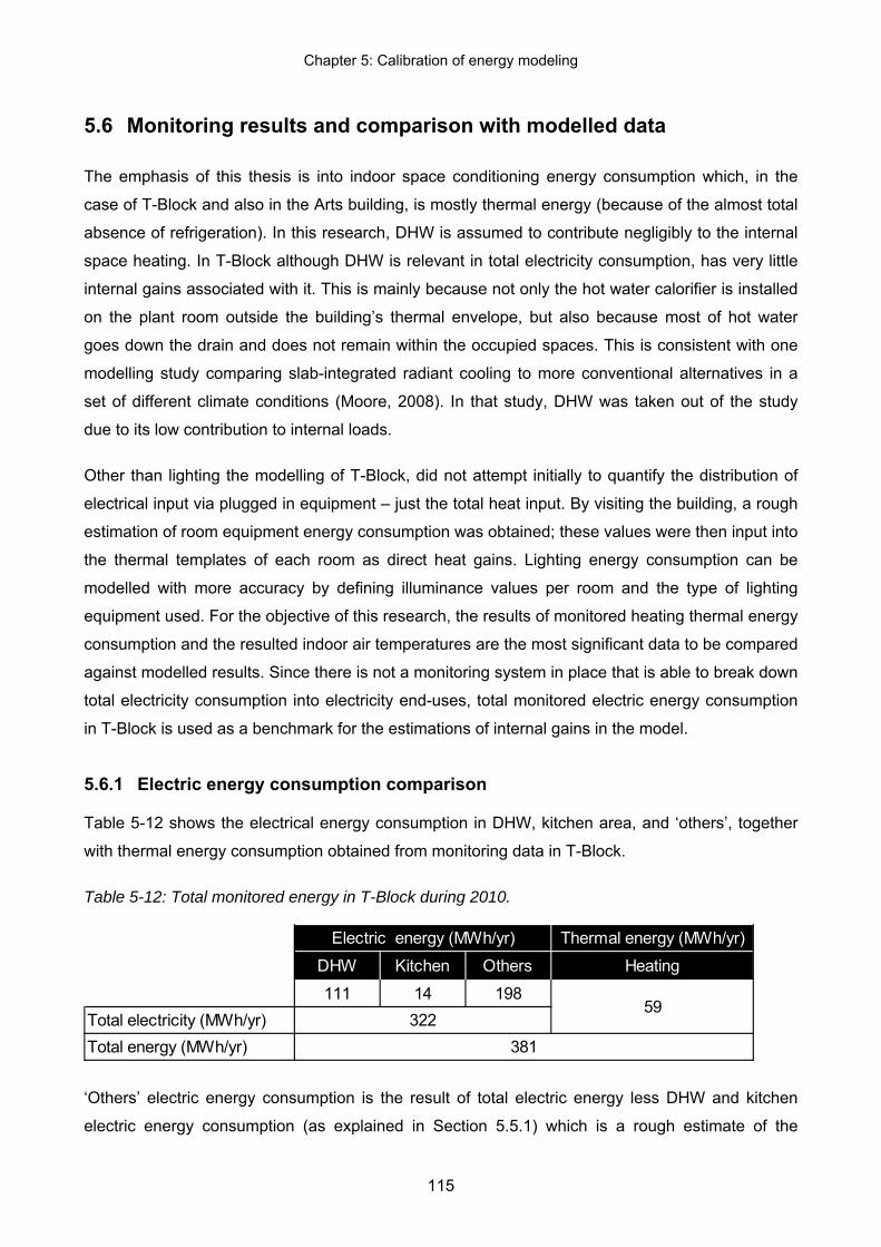
Chapter 5: Calibration of energy modeling
115
5.6 Monitoring results and comparison with modelled data
The emphasis of this thesis is into indoor space conditioning energy consumption which, in the
case of T-Block and also in the Arts building, is mostly thermal energy (because of the almost total
absence of refrigeration). In this research, DHW is assumed to contribute negligibly to the internal
space heating. In T-Block although DHW is relevant in total electricity consumption, has very little
internal gains associated with it. This is mainly because not only the hot water calorifier is installed
on the plant room outside the building’s thermal envelope, but also because most of hot water
goes down the drain and does not remain within the occupied spaces. This is consistent with one
modelling study comparing slab-integrated radiant cooling to more conventional alternatives in a
set of different climate conditions (Moore, 2008). In that study, DHW was taken out of the study
due to its low contribution to internal loads.
Other than lighting the modelling of T-Block, did not attempt initially to quantify the distribution of
electrical input via plugged in equipment – just the total heat input. By visiting the building, a rough
estimation of room equipment energy consumption was obtained; these values were then input into
the thermal templates of each room as direct heat gains. Lighting energy consumption can be
modelled with more accuracy by defining illuminance values per room and the type of lighting
equipment used. For the objective of this research, the results of monitored heating thermal energy
consumption and the resulted indoor air temperatures are the most significant data to be compared
against modelled results. Since there is not a monitoring system in place that is able to break down
total electricity consumption into electricity end-uses, total monitored electric energy consumption
in T-Block is used as a benchmark for the estimations of internal gains in the model.
5.6.1 Electric energy consumption comparison
Table 5-12 shows the electrical energy consumption in DHW, kitchen area, and ‘others’, together
with thermal energy consumption obtained from monitoring data in T-Block.
Table 5-12: Total monitored energy in T-Block during 2010.
Thermal energy (MWh/yr)
DHW Kitchen Others Heating
111 14 198Total electricity (MWh/yr)Total energy (MWh/yr)
59322
381
Electric energy (MWh/yr)
‘Others’ electric energy consumption is the result of total electric energy less DHW and kitchen
electric energy consumption (as explained in Section 5.5.1) which is a rough estimate of the

Chapter 5: Calibration of energy modeling
116
electric energy consumption of conventional electric energy end-uses such as lighting, equipment
and mechanical ventilation for areas of the building not included in the kitchen electric distribution
board. Figure 5-10 is a comparison between monitored and modelled total electric energy, also
included is the monitored and modelled total electric energy with DHW and kitchen area electricity
subtracted out (‘Others’ in Table 5-12). It is this net electric energy consumption that was used for
the estimation of internal gains for modelling of thermal energy consumption.
0
1
2
3
4
5
6
7
8
9
10
1 3 5 7 9 11 13 15 17 19 21 23 25 27 29 31 33 35 37 39 41 43 45 47 49 51
MW
Total Elec. MONITORED Total Elec. No (DHW & Kitchen) MONITOREDTotal Elec. MODELLED Total Elec. No (DHW & Kitchen) MODELLED
Figure 5-10: Total Electricity consumption + DHW Energy consumption
The actual values of monitored and modelled total electric energy consumption compared with
‘Others’ electric energy consumption is given in Table 5-13. To achieve the similarity between
monitored and modelled values in Table 5-13, modelled electric energy consumption had to be
increased by adding extra equipment electricity consumption (about 20 W/m2) to all spaces which
subsequently increased internal gains. This is a very simplified approach to deal with the
uncertainty of real internal gains generated by conventional electric energy end-uses.

Chapter 5: Calibration of energy modeling
117
Table 5-13: Summary comparison between metered and modelled data
Total Elec. Total Elec. No (DHW & Kitchen)
Total Elec. Total Elec. No (DHW & Kitchen)
MONITORED MONITORED MODELLED MODELLEDAverage (kW) 6.2 3.8 5.9 3.3Max (kW) 9.3 5.5 9.4 5.9Total (MWh) 322 198 308 169
5.6.2 Thermal energy consumption comparison
A comparison between monitored and modelled weekly heating thermal energy consumption, can
be seen in Figure 5-11. Weekly average outdoor air temperature is also included to identify the
influence of climate conditions on heating energy consumption.
0
5
10
15
20
25
0.0
0.5
1.0
1.5
2.0
2.5
3.0
3.5
4.0
4.5
5.0
1 3 5 7 9 11 13 15 17 19 21 23 25 27 29 31 33 35 37 39 41 43 45 47 49 51
Te
mp
era
ure
(C
)
MW
Heating (MW) MONITORED Heating (MW) MODELLED Outdoor Temperature (C )
Figure 5-11: Heating thermal energy consumption - comparison between monitored and modelled
data.

Chapter 5: Calibration of energy modeling
118
In Section 5.3.1 (Table 5-5) the annual templates used for the energy modelling of T-block were
given. Heating thermal energy is provided by a centralized boiler operating during winter only, from
the May 6 until October 29, which is evident in Figure 5-11 where heating started on week 18 (May
03 – 09) and ended on week 44 (October 25 – 31). Two of NMIT’s four study breaks lie within this
heating period (there are 3 study break of two weeks each, and one long summer break of about
14 weeks). The two study breaks during the heating season were on Weeks 27 and 28 and Weeks
40 and 41; these weeks are highlighted with a vertical segmented line in Figure 5-11. The influence
of the two study breaks into the heating consumption is also evident as a reduction in heating
consumption in both monitored and modelled heating energy consumption patterns. Since values
in Figure 5-11 are weekly averages, these show a reduction of heating consumption in both weeks
of both of the study breaks where, although internal gains were reduced by low occupancy, none of
the openable windows were operable during these periods in both the monitored and modelled
building.
There is a peak of heating energy consumption in Week 31, two weeks after the first study break,
this occurred simultaneously with low outdoor dry-bulb air temperature (peak low on Week 28).
The cooling down of the thermal mass of the building during the study breaks also might have an
influenced in the heating peak on Figure 5-11; this will be discussed further when weekly average
indoor temperatures in T-Block are analysed in the next section.
In summary the analysis of heating thermal energy some key values are informative. The average
weekly monitored thermal energy consumption is 1.1 MWh compared with the model in which the
value is 1.0 MWh. The maximum weekly monitored thermal energy consumption is 4.4 MWh
compared with modelled values of 4.7 MWh. Finally the total thermal energy consumption in
heating is 58.7 MWh in the monitored data compared with a 51.1 MWh in the modelled building.
5.6.3 Air Temperature comparison in T-Block
Each of the six rooms in T-Block which have air temperature monitoring equipment installed can be
seen in Section 5.5 (Figure 5-9) where Level 1, Level 2, and Level 3 are presented, each level with
two rooms highlighted in grey, one room facing north and the second one facing south (exception
of room 1B in Level 1 which face south west). By monitoring thermal conditions in rooms exposed
to north compared to rooms facing south, the monitoring system is giving a range of indoor air
temperature across each floor.
For each of the rooms in Figure 5-9, a comparison between monitored and modelled average,
maximum, and minimum temperature is given in Table 5-14. Also included are the monitored and
modelled values of median temperature, and their respective standard deviations.

Chapter 5: Calibration of energy modeling
119
Table 5-14: Summary of T-Block room’s temperature data analysis.
Monit. Mod. Monit. Mod. Monit. Mod. Monit. Mod. Monit. Mod. Monit. Mod.Average 21.6 22.2 22.5 19.8 22.5 21.7 21.8 19.9 21.3 21.7 21.4 20.3Max 28.9 30.2 27.8 29.2 28.0 31.3 28.2 27.1 29.8 32.6 32.2 30.9Min 13.4 13.4 15.3 9.4 17.0 12.1 14.5 11.5 13.3 10.2 11.0 8.3Median 21.8 22.3 22.5 20.6 22.6 21.7 21.6 20.0 21.3 21.7 21.1 21.0Standard Dev. 2.3 2.8 2.0 3.4 1.7 3.3 2.3 2.7 2.4 3.7 3.5 3.9
Training Kitchen (1A)
Restaurant (1B)
L 1 - North L1 - South L 2 - North L2 - South
Staff Room (2A)
Beauty Salon (2B)
Classroom (3A)
Classroom (3B)
L 3 - North L3 - South
There is no consistent pattern when the monitored and modelled maximum temperatures are
compared: in four of the rooms the modelled maximum exceeds the monitored maximum while in
two rooms (both south-facing) the modelled maximum is less than the monitored maximum. For
the minimum temperatures, however, the modelled minimum never exceeds the monitored
minimum (they are equal for the training kitchen) with the greatest extreme case arising in the
restaurant (15.3°C monitored minimum compared with 9.4°C modelled minimum). When
combined, these observations imply that, in general, the model is predicting larger diurnal
temperature swings than have been recorded by the monitoring equipment. Of relevance to this, as
noted in Section 3.9.2, (Pereira & Ghisi, 2011) reported simulation peak temperature differences
exceeded measured values (by about 2°C) in their investigations.
Because, by definition, maximum and minimum temperatures are extreme and short-duration
occurrences, any significant differences between monitored and modelled values of these
temperatures will not automatically translate into significant differences between the monitored and
modelled energy consumption figures, nor indeed into significant differences in thermal comfort
(particularly since minimum temperatures occur outside occupied hours).
Hence a more meaningful basis for comparing the model’s temperature predictions with the
monitored values is to observe the average temperatures (first line of Table 5-14) since, to a first
approximation, it is the average indoor-outdoor temperature difference which primarily governs the
rate of energy loss from a building having a given thermal envelope. Here the modelled/monitored
values compare more favourably, the modelled value being higher for two rooms (0.6°C for the
kitchen) and lower for four rooms (2.7°C for the restaurant is the most extreme difference). It is
possibly not a coincidence that the restaurant is the same room for which the discrepancy on the
minimum temperature was greatest.
The degree of agreement of the monitored and modelled median temperatures (fourth line of
Table) is the most encouraging and arguably the most meaningful because, by effectively raising

Chapter 5: Calibration of energy modeling
120
the statistical influence of the most commonly encountered temperatures, it lessens the influence
of the most extreme excursions (i.e. maxima and minima). As already noted above, these
extremes – particularly the minima – do not appear to have been well represented in the model.
From the median temperature perspective, four of the rooms have monitored/modelling agreement
within 1°C (two with monitored higher than modelled – Classroom 3B by only 0.1°C - and two with
it being lower) while, again, it is the restaurant showing the largest discrepancy (monitored
temperature 1.9°C higher than modelled). As an approximate single value indicator of the degree
of agreement between monitored and modelled temperatures, when the differences for the six
monitored rooms are averaged, the resulting value of 0.6°C is not too dissimilar from the mean
difference of 0.4°C reported by (Pereira & Ghisi, 2011) in their measured/simulated comparison.
Indoor air temperature fluctuation about the average values can also be observed by looking at
whole year hourly temperature’s standard deviation in Table 5-14. Modelled indoor air temperature
has, in all rooms, a higher standard deviation than monitored air temperatures regardless of the
orientation of the room. This is consistent with the observation above that the model is predicting
larger diurnal temperature swings than have been recorded by the monitoring equipment.
Differences in standard deviation between monitored and modelled north-facing room’s indoor
temperature range from 0.5°C in Level 1 to 1.6°C in Level 2. In south-facing rooms, differences on
standard deviation between monitored and modelled south-facing room temperatures range from
about 0.4°C in Level 3 to 1.3°C in Level 1.
5.6.4 Indoor air temperature in Level 1, Level 2, and Level 3
In the energy modelling of T-Block, emphasis was given to modelling rooms in Level 2 to the best
possible accuracy. Since the emphasis of this thesis is into the influence of thermal mass into
space conditioning energy consumption, by focussing on the analysis of air temperatures in Level
2 the influence of the particular structural fabric of T-Block will be most evident. This is because
Level 2 is a space supported within concrete suspended floors enclosed by a light weight insulated
envelope, compared with Level 1 where the indoor environment might be highly influenced by the
massive concrete slab on ground, or in Level 3 where the there is a lightweight roof and thermal
envelope in general, without any consistent source of thermal mass other than the suspended floor
below. Also, because Level 2 has a lower area of the building’s thermal envelope than Level 1 and
Level 3, heat losses can be expected to have a smaller influence on the results that this research
is looking for. Nevertheless, it is appropriate that the monitored and modelled temperatures from
Levels 1 and 3 be considered as well, and these will be commented on first.
Figure 5-12 shows the two rooms fitted with air temperature sensors in Level 1 (the training kitchen
in (a) and the restaurant in (b)), and in Level 3, a picture of the general classroom facing north (c).

Chapter 5: Calibration of energy modeling
121
The training kitchen is a large open space (no internal partitions) equipped with cooking
equipment, lighting and mechanical air supply and extraction systems via kitchen hoods.
Occupancy in this room is not constant and varies between periods of low and very high
occupancy.
(a) (b) (c)
Figure 5-12: Rooms with air temperature monitoring equipment in the training kitchen (a), and
restaurant (b) in Level 1, and in a general classroom (c) in Level 3.
The restaurant (Picture (b)) is a room heavily exposed to the building’s thermal envelope where
mostly large panes of single glazing is used; it has low occupancy during the day and very high
during afternoons and evenings. The general classroom in picture (c) is exposed to the north
façade, and the other Level 3 room with an air temperature sensor is visually similar. Level 3 has a
light weight construction structured in steel columns and beams, with the only significant source of
thermal mass being in the concrete suspended floor system which, in both rooms, is covered with
carpet. There are no differences between insulation values in the external walls and in the roof,
both being about R 2.5.
4
8
12
16
20
24
28
1 5 9 13 17 21 25 29 33 37 41 45 49
Tem
pera
ture
(C
)
Room 1A - Training Kitchen north
1A Monitored 1A Modelled Outdoor Temperature (C ) (a)
4
8
12
16
20
24
28
1 5 9 13 17 21 25 29 33 37 41 45 49
Room 1B - Restaurant south
1B Monitored 1B Modelled Outdoor Temperature (C ) (b)
Figure 5-13: Weekly averaged room air temperature in rooms on Level 1 - the training kitchen (a)
and restaurant (b).
The weekly average monitored and modelled air temperatures for the training kitchen and for the
restaurant are labelled as (a) and (b) in Figure 5-13, (which is consistent with what’s been done in
other figures). The three short study breaks and also the long summer break are again indicated

Chapter 5: Calibration of energy modeling
122
with vertical segmented lines located at the beginning and at the end of each study break. (For the
long summer break, the line at Week 48 indicates the beginning of the break in November and the
line at Week 5 indicate the end of the summer break in February).
Monitored and modelled air temperatures in the training kitchen show generally good agreement
with the modelled average weekly temperature almost consistently being slightly below the
monitored equivalent. When the magnitude of this discrepancy is compared with the overall inside-
outside temperature difference in Figure 5-13 (a), however, it can be deduced that the overall
impact on the accuracy of modelling predictions of the energy required to maintain that inside-
outside temperature difference should be small. For the restaurant a much larger gap exists
between the monitored and modelled temperature profiles, with the monitored temperatures being
consistently higher. Contributing to this is the already noted fact that for this room the model
predicted a much lower minimum temperature than that which was monitored. Two software-
related constraints may explain the apparently poor modelling of the restaurant: Firstly the software
was unable to vary occupancy density during one given day and instead used one constant low
occupancy density. Secondly, the restaurant has thick curtains installed but these were not
thermally modelled because of the complexity of their intermittent use). These curtains would
reduce the heat losses through the large single glazed windows, particularly at night time when the
minimum temperatures would occur.
The weekly average monitored and modelled air temperatures of the general classroom facing
north and general classroom facing south on Level 3 are shown in Figure 5-14.
4
8
12
16
20
24
28
1 5 9 13 17 21 25 29 33 37 41 45 49
Tem
pera
ture
(C
)
Room 3A - Classroom north
3A Monitored 3A Modelled Outdoor Temperature (C ) (a)
4
8
12
16
20
24
28
1 5 9 13 17 21 25 29 33 37 41 45 49
Room 3B - Classroom south
3B Monitored 3B Modelled Outdoor Temperature (C ) (b)
Figure 5-14: Weekly averaged room air temperature in rooms on Level 3 - the general classroom
facing north (a) and facing south (b).
In all four graphs in Figure 5-13 and Figure 5-14 the influence of study breaks is apparent in the
indoor temperatures of both monitored and modelled data (though less clear in the restaurant) with

Chapter 5: Calibration of energy modeling
123
an anticipated and consistent decrease of air temperature during these breaks in both the
monitored and modelled data.
There is evidence of the agreement between monitored and modelled temperatures having a
dependence on room orientation. Particularly in Figure 5-14 it can be seen that air temperature
variation between summer and winter is higher in rooms facing south compared with rooms facing
north. In this same figure, monitored air temperature in room 3B facing south is often higher than
the modelled air temperature during the whole year, but in the same figure, in room 2A facing
north, monitored air temperature is often higher than modelled air temperature during cold, and
lower during warmer periods of the year. In Table 5-14 in rooms facing north, modelled maximum
temperature is 1.3°C to 3.3°C higher than monitored maximum temperatures, while in rooms facing
south, modelled maximum temperature is about 1.5°C lower than monitored maximum
temperatures. In rooms facing north, modelled minimum temperature is about 4°C lower than
monitored minimum temperature, while In rooms facing south, modelled minimum temperature is
3°C to 6°C lower than monitored minimum temperatures.
Summarising all of the preceding comments on the data presented in Table 5-14, Figure 5-13 and
Figure 5-14: Looking at average weekly values throughout a whole year, although average
temperatures are similar in real building and models, air temperature swings are much higher in
the models. In rooms facing north, the influence of outdoor air temperature on indoor air
temperature is lower than in rooms facing south and, particularly in this orientation, modelled
temperatures are considerably lower throughout the whole year than monitored air temperatures.
In rooms facing north monitored and modelled air temperatures are of a much greater similarity.
5.6.4.1 Indoor air temperature in Level 2 - detailed temperature analysis
(a) (b) (c)
Figure 5-15: Level 2 Staff room – Picture (a) north facing windows, picture (b) total office overview,
and picture (c) air temperature sensor location.
In the two rooms with air temperature sensors located in Level 2, the exact location of the sensor
has been identified. In Figure 5-15 a sequence of three pictures of the Staff Room (2A) on the
north façade of Level 2, can be seen. The size of the room and density of occupancy can be
appreciated in a panoramaic view produced by pictures (a) and (b); also in picture (b) the exact

Chapter 5: Calibration of energy modeling
124
location of the air temperature sensor can be appreciated (inside a red circle). A detailed view of
the air temperature sensor can be seen in picture (c).
To reduce uncertainty about the accuracy of the method used for comparison between monitored
and modelled indoor air temperatures, and to assess if the comparison clearly captures the
influence of HVAC systems on indoor air temperature, a comparison has been made between
whole year weekly average air temperature of buildings during 24 hours (i.e. both occupied and
unoccupied hours), and the building’s occupied hours only (8:00am to 6:00pm). This comparison is
shown in Figure 5-16. While monitored air temperature remains constant in both graphs, modelled
air temperature varies significantly between graphs. Since there is a large variation of temperature
between day and night during a 24 hour period, particularly in the modelled air temperature (see
analysis of Table 5-14 and Figure 5-13 and Figure 5-14), when reducing the extent of data
included in the graphs, from 24 hours to occupied hours only, the significant drop of temperature
during night time is not integrated into the average value, which subsequently produces a
significantly higher total average value. Average monitored air temperature, over occupied hours
only is 0.4°C higher than the same value over a 24 hour period. In the case of average modelled
temperature of occupied hours is 2.3°C higher than monitored averaged values over 24 hours.
14
16
18
20
22
24
26
28
30
1 5 9 13 17 21 25 29 33 37 41 45 49
Tem
pera
ture
(C)
Weekly averaged over a 24 hours day
2A Monitored -24h 2A Modelled-24h 2A Occupancy(a)
14
16
18
20
22
24
26
28
30
1 5 9 13 17 21 25 29 33 37 41 45 49
Weekly averaged over daily occupied hours only
2A Monitored-10h 2A Modelled-10h 2A Occupancy(b)
Figure 5-16: Room 2A north - Average weekly air temperature (a), and average weekly air
temperature for building’s occupied hours only (b).
A comparison between half hour monitored and modelled indoor air temperatures during one week
in the study break (5-11 April), and one week in the middle of the second semester (August 30 to
September 5) can be seen in Figure 5-17. Graphs in Figure 5-17 are representative of one week
without heating and – nominally – no occupation, lighting, and equipment internal gains (a), and
one week with heating, occupation, lighting, and equipment internal gains (b). It can be seen in
Figure 5-17 that when the building is unconditioned and unoccupied (a), modelled indoor air
temperature during the day is close to but consistently below the monitored data. During the night
modelled temperatures drop significantly in comparison with monitored temperatures during the

Chapter 5: Calibration of energy modeling
125
same period so that, overall, the model’s over-estimation of the diurnal swing is once again
apparent. When the building is heated and occupied (Figure 5-17 (b)), indoor air temperature
during the day the modelled temperature profile clearly exceeds the monitored temperature profile
(with the exception of the last day which is an unoccupied Sunday), and during the night modelled
temperatures again drop significantly when compared with monitored data, following the trend that
night temperature does in (a).
14
16
18
20
22
24
26
28
30
5/04
/201
0…
6/04
/201
0…
7/04
/201
0…
8/04
/201
0…
9/04
/201
0…
10/0
4/20
10…
11/0
4/20
10…
Tem
pera
ture
(C)
Weekly Room 2A - 1st study break (no heating & occupancy)
2A Monitored 2A Modelled (a)
14
16
18
20
22
24
26
28
30
30/0
8/20
10…
31/0
8/20
10…
1/09
/201
0…
2/09
/201
0…
3/09
/201
0…
4/09
/201
0…
5/09
/201
0…
Tem
pera
ture
(C)
Weekly Room 2B - End of august (with heating & occupancy)
2A Monitored 2A Modelled (b)
Figure 5-17: For Room 2A (north), half hour temperature graph for one week without heating and
general occupancy (a), and one week with heating and general occupancy (b).
Temperatures profiles in modelled conditioned and unconditioned indoor environment are offset
profiles to outdoor dry-bulb temperatures. This is not the case when looking at monitored indoor
environments where temperatures are more stable during day and night and less influenced by
outdoor dry bulb temperature. This can be seen more in detail in Figure 5-18 where there are two
graphs with one day of half hour recorded temperature in room 2A during an unheated and
unoccupied day (a) compared with the same room during a heated and occupied day (b). Also
included in both graphs in Figure 5-18 is the hourly outdoor dry-bulb temperature.
4
8
12
16
20
24
28
0:15 6:15 12:15 18:15
Tem
pera
ture
(C)
Daily Room 2A - 1st study break (no heating & occupancy)
2A Monitored 2A Modelled Dry-bulb temperature ( C) (a)
4
8
12
16
20
24
28
0:15 6:15 12:15 18:15 0:15
Tem
pera
ture
(C)
Daily Room 2A - September (With heating & occupancy)
2A Monitored 2A Modelled Dry-bulb temperature ( C) (b)
Figure 5-18: For Room 2A (north), half hour temperature graph for one day without heating and
general occupancy (a), and one day with heating and general occupancy (b).

Chapter 5: Calibration of energy modeling
126
Figure 5-18 shows that monitored air temperature is less responsive to outdoor air temperatures
and also to conditioning heat than modelled temperature is. Whenever there is a heat input, the
modelled temperature responds faster and increases to a higher level than the monitored
temperatures. Similarly when there is no heat input and the outdoor temperature drops, the
modelled indoor temperature drops more quickly and to a lower level than the monitored data.
This greater responsiveness of indoor temperature to outdoor conditions and to space conditioning
in the model could be due to a number of reasons but these have not been tested or analysed in
detail from a temperature perspective because they are outside the primary scope of this research.
In the Test building analyses in Section 3.11, however, the energy consumption consequences of
significant changes in the amount and accessibility of thermal mass was explored. The conclusion
that was reached there was that the energy usage was only minimally effected by those changes in
that Test building at least. This is somewhat reassuring in the present context because it suggests
that over-estimation of diurnal temperature swing – which would normally be associated with a low
amount of accessible thermal mass – should not have significant flow-on consequences in
modelling the operational energy consumption of the building during occupied hours. Nevertheless,
some possible factors contributing to the model’s over-estimation of diurnal temperature swing are:
Since the monitored building is relatively new, it is under-occupied, so day-time internal
gains may be less than actually modelled.
Natural ventilation – which was not able to be measured or monitored – may not occur to the
extent that is assumed in the model.
5.6.4.2 Indoor air temperature in Room 2A and 2B in Level 2 - detailed temperature analysis
The indoor air temperature in the staff room (2A) facing north can be seen in Figure 5-19 and for
the beauty salon (2B) facing south can be seen in Figure 5-20. Each of the temperature traces in
these figures is tracking the weekly variation in the particular temperature, with each data point
being the average of the temperature values obtained on an hourly basis during that week (i.e the
average of 168 values per week, either monitored or modelled). Included in the analysis
capabilities of the VE software is the ability to extract temperature profiles for internal room
surfaces of interest. This capability has been utilised to clarify whether or not the surface
temperature of the walls where the temperature sensors are located, has an influence on the
monitoring of temperature, hence the modelled surface temperature of the wall at each sensor’s
location has been included in the graphs.

Chapter 5: Calibration of energy modeling
127
5
10
15
20
25
30
1 5 9 13 17 21 25 29 33 37 41 45 49
Tem
pera
ture
(°C
)
2A Monitored 2A - Wall Modelled 2A - Air ModelledOccupancy Outdoor Temperature (C°)
Figure 5-19: Room air temperature – Level 2 Staff Room – North facing.
5
10
15
20
25
30
1 5 9 13 17 21 25 29 33 37 41 45 49
Tem
pera
ture
(°C
)
2B Monitored 2B - Wall Modelled 2B ModelledOccupancy Outdoor Temperature (C°)
Figure 5-20: Room air temperature – Level 2 Beauty – South facing

Chapter 5: Calibration of energy modeling
128
Figure 5-19 and Figure 5-20 show that differences between indoor air temperature and wall
surfaces temperature are more marked in the room on the south façade than in the room on the
north. In both, the south and the north facing rooms, the wall surface temperature is always higher
than indoor air temperature.
On the north façade, indoor air temperature and wall surface temperature are very similar with
differences that increase during summer months and peaks up to 0.5°C during December and
January. On the south façade, indoor air temperature and wall surface temperature have higher
difference than those in the north facing room, ranging from 0.1 to 1.1°C difference with peak
difference in month of February and March.
Figure 5-13 and Figure 5-14 showed that modelled indoor temperatures are lower than measured
indoor temperature in the rooms facing south. In rooms facing north, most of the time modelled
indoor temperature is higher than measured indoor temperatures, there being only a few weeks in
winter where modelled indoor temperature is lower than measured indoor temperature.
Figure 5-19 and Figure 5-20 show that measured indoor air temperature is normally higher than
modelled indoor air temperature in the north and always higher in the south. These figures also
show that a wall surface temperature (of the wall where the temperature sensor is located) is
higher than indoor air temperature. This suggest that there may be an influence of the surface
temperature of the wall where the sensor is located on the measurements this sensor is detecting,
increasing the final measurement of indoor air temperature by the sensor. Overall, however, this
influence is relatively small and doesn’t account for more than a small fraction of the largest
modelled/monitored temperature difference (for the north-facing Staff Room 2A at Week 29,
immediately after the mid-year break).

Chapter 6: Assessment of the accuracy of energy modeling in the Arts building
129
6 Assessment of the accuracy of energy modelling in the Arts building
This chapter describes a simplified calibration process undertaken in the Arts building, to be used
as the primary case-study building, later the template for all the alternative case-study building
models. A description of a monitoring system designed and installed in that building is given. The
chapter includes a comparison of monitored and modelled indoor temperatures. In the case of
energy consumption (for which meaningful monitored data was not available), a comparison with
other broadly similar educational buildings is described, to give an order of accuracy for the
modelling results in the remaining chapters.
6.1 Introduction
An energy and indoor temperature monitoring system was designed for the Arts building. The aim
of this monitoring system was two-fold: to calibrate the BEEM modelling undertaken in this
research; and to obtain meaningful on-going information for future research in this building (bearing
in mind that it is the first multi-storey timber building of this nature built in New Zealand).
The energy and temperature monitoring equipment was installed in the Arts building during late
2010 and beginning of 2011. The commissioning of the building was carried out during January
2011 and occupancy started mid-February 2011. The first metering data for both energy
consumption and indoor temperatures was received on February 22.
Due to complications and unreliability in the monitoring of thermal and electrical energy
consumption, that data and its subsequent comparison with the BEEM modelling results were not
able to be included in this research. Only indoor temperature comparisons are included.
This section describes the design of the monitoring system for thermal and electrical energy
consumption in the Arts building, together with a set of room air temperatures in the same building.
This section also introduces some of the room air temperature monitoring results and compares
them with modelled temperatures.
6.2 Brief description of monitoring system in the Arts building
The Arts building is part of group of three buildings at NMIT, called the Arts and Media complex.
Figure 6-1 (a) shows the plan section of the three buildings that form the Arts and Media complex,
being the three storey tall Arts building (hatched (a -1)), the single storey workshop building (a - 2)
and the ‘Performance’ space (a - 3). Figure 6-1 (b) shows the west elevation of the Arts and Media

Chapter 6: Assessment of the accuracy of energy modeling in the Arts building
130
complex where the buildings height can be appreciated – particularly the three storey tall Arts
building (b-1).
Thermal and electric energy are supplied to the Arts and Media complex as a whole. In the case of
electricity this is supplied to a central electric board (main) in the Arts building and redistributed to
the sub-boards, one in the workshop building and another to the Performance building. There is a
similar situation with thermal energy used in LPHW for heating. This is supplied to the Arts building
and redistributed to the workshop and the Performance buildings. A problem with this layout of
electricity and LPHW distribution is that to extract meaningful data for the Arts building alone, this
has to be isolated from main electric energy consumption (total Arts and Media complex) less
electric consumption of the workshop and of the Performance space (each having a sub-board).
The same approach has to be taken to individualize the thermal energy consumption in the Arts
building.
(a) (b)
Figure 6-1: Layout of Arts and Media complex – Plan section in (a) and west elevation in (b)
As for the T-Block, temperature monitoring equipment has been installed previously to feed into the
BMS for controlling the temperature of air supplied by the air handling unit, and scheduling the
opening of windows located in the thermal envelope for natural ventilation. The same company
specialising in energy management was in charge of the design and the installation of the system
(Schneider Electric, 2011). In Table 6-1 the energy monitoring points for the Arts and Media
complex (a) and the temperature monitoring points for the Arts building (b) are summarized.
a - 2
a - 1
a - 3
b - 2 b - 1 b - 3
N

Chapter 6: Assessment of the accuracy of energy modeling in the Arts building
131
Table 6-1: List of monitoring equipment for energy in the Arts and Media complex (a) and
temperature in the Arts building (b).
EnergyThermal (3 storey building)
1 Main Heat Energy2 Workshop Heat Energy3 AHU1 Heat Energy
Electric (3 storey building)4 Main Board Elec Energy5 Workshop Elec Energy6 Performance Elec Energy
Other Electric 7 AC1 AC2 Cool Energy8 AHU3 Elec Energy
(a)
TemperatureRoom Air Temperature:
1 Level 1 Multimedia102 Room Temp2 Gallery103 Room Temp (RM104)3 Reception Room Temp (RM 109 - RM110)4 Interview (RM113) & HOS (RM114) Avg Room Temp5 ProgLeader Kitch Avg Room Temp.6 Level 2 Studio201 Room Temp7 Main Gallery Avg Room Temp (Level 2 ?)8 Level 3 Studio301 Room Temp9 Workroom302 Room Temp10 Workroom303 Room Temp11 Classroom304 Room Temp
Other Temperatures:12 OSA Temp (Outside Air Temperature) (b)
For this research, thermal energy from the campus heating system was the most significant energy
being monitored because it represents virtually all of the heating energy input. However, there
were problems in the monitoring of the hot water energy and the commissioning of that system is
still on-going. Because LPHW flow had to be monitored at three points and LPHW temperature
difference had to be monitored in and out of three zones (one for the complex of three buildings
and two representing sub-buildings), the inherent potential inaccuracies of obtaining quantities by
subtraction between separate measurements was very apparent in the limited data that was able
to be obtained. Thus no meaningful data was able to be extracted before this research was
drawing to a close. Although electric energy has been monitored, the accuracy of total electricity
energy consumption is not the main objective of this research and, because the heat input via hot
water was not able to be obtained, the electricity consumption has not been analysed further.
6.3 Benchmark of the modelled heating energy consumption in the Arts building
In the absence of meaningful data from the hot water monitoring system, this section presents the
results of the modelled heating energy consumption in the actual Arts building and compares that
result with heating energy consumption from a set of three educational buildings in New Zealand.
Buildings used in this comparison are the T-Block in NMIT’s Nelson campus, and the Erskine and
the Rutherford buildings at the University of Canterbury (UoC) main campus in Christchurch, New
Zealand. Rather than being a detailed analysis of heating energy consumption in educational
buildings in New Zealand, this benchmarking is intended to provide a relative idea of the accuracy
of the heating modelling in the Arts building.

Chapter 6: Assessment of the accuracy of energy modeling in the Arts building
132
Table 6-2: Gross and usable area of building used to benchmark heating energy comparison in the
Arts building.
Gross (m2)
Usable (m2)
Gross (m2)
Usable (m2)
Gross (m2)
Usable (m2)
Gross (m2)
Usable (m2)
1,981 1,693 2,068 1,991 11,551 5,244 19,368 10,356
Arts Bldg.Nelson Marlborough Institute of Technology (NMIT) University of Canterbury (UoC)
T-Block Erskine Rutherford
Table 6-2 provides the areas of the four buildings compared in this section. The Arts building is the
smallest building in this comparison but is close in size to the T-Block (NMIT). Buildings in the
University of Canterbury campus on the other hand are much bigger. The comparison of the Arts
building with the T-Block is a straightforward comparison between buildings in the same location,
with similar usage, thermal envelope and structural thermal mass. The choice of buildings at the
University of Canterbury is because these two buildings represent both ends of the spectrum: the
much more modern Erskine building has relatively low heating energy consumption whereas the
Rutherford building has relatively high heating consumption.
Figure 6-2: Erskine building at the University of Canterbury.
The Rutherford building is an eight-storey reinforced concrete building, built in 1967, and holds the
departments of Chemistry and Physics of UoC. The building includes classrooms, lecture theatres
and a large area assigned to laboratories. The Erskine building (Figure 6-2) is a complex building
with 3 seven-storey office buildings attached to a central atrium that, at the same time, connects
the buildings to a library and to computer labs. It is a reinforced concrete building built in 1996 for
the Departments of Mathematics and Statistics, and Computer Science. Concepts of

Chapter 6: Assessment of the accuracy of energy modeling in the Arts building
133
Environmental Sustainable Design (ESD) were included in the design of the Erskine building and
the building is regarded as a low-energy building within the UoC campus.
Table 6-3 shows the monthly thermal energy consumption subdivided in gross and usable floor
area of the buildings in this comparison. Data in the T-Block and in the Erskine and Rutherford
building was monitored during the year 2010 rather than 2011 because 2011 was an abnormal
year for UoC campus energy usage due to the disruptions caused by major earthquakes. Data for
the Arts building is modelled using a TMY weather file. Energy in both buildings in the UoC campus
was provided by the campus Facilities Manager (Sellin, 2011), and the values given include
heating and DHW added together (although the latter is expected to be a small portion of the total
energy consumption value compared with heating energy consumption.
As it can be seen in this table, when the heating energy consumption is expressed on a per unit
gross floor area basis, the modelled heating energy consumption of the Arts building is similar to
the metered heating energy consumption in the T-Block and the Erskine building, and much lower
than the heating energy consumption in the Rutherford building. When looking at heating energy
consumption divided by usable floor area, the modelled heating energy consumption in the Arts
building is, again, similar than the metered heating energy consumption of the T-Block, but
significantly lower than the energy consumption of each of the two buildings in the UoC campus.
Table 6-3: Thermal energy consumption on heating of the Arts building - Comparison between
monitored and modelled
Gross (kWh/m2)
Usable (kWh/m2)
Gross (kWh/m2)
Usable (kWh/m2)
Gross (kWh/m2)
Usable (kWh/m2)
Gross (kWh/m2)
Usable (kWh/m2)
Jan 0.0 0.0 0.0 0.0 0.0 0.0 0.0 0.0Feb 0.0 0.0 0.0 0.0 0.1 0.2 0.6 1.2Mar 0.0 0.0 0.0 0.0 0.6 1.2 3.3 6.2Apr 0.0 0.0 0.0 0.0 1.5 3.3 5.6 10.4May 3.5 4.1 2.4 2.5 4.7 10.3 13.6 25.4Jun 6.1 7.1 6.3 6.3 9.1 20.0 15.6 29.2Jul 7.8 9.1 7.2 7.5 8.7 19.1 14.9 27.9
Aug 6.5 7.6 5.8 6.0 8.4 18.4 15.5 29.0Sep 4.1 4.8 4.8 5.0 4.6 10.1 9.3 17.4Oct 3.0 3.6 2.2 2.3 3.0 6.6 7.2 13.4Nov 0.0 0.0 0.0 0.0 4.6 10.1 9.3 17.4Dec 0.0 0.0 0.0 0.0 0.0 0.0 0.0 0.0
∑ 31.1 36.4 28.4 29.5 45.1 99.3 94.9 177.5
Arts Bldg. - Mod.NMIT - Nelson UoC - Christchurch
Rutherford - Met.Erskine - Met.T-Block - Met.

Chapter 6: Assessment of the accuracy of energy modeling in the Arts building
134
Significant differences between heating energy consumption when subdivided into gross and
usable area in the Erskine building (UoC) and, to a lesser extent, to the Arts building (NMIT) may
be attributed to the influence of the large atrium space within those buildings, which although the
whole atrium space is conditioned, this large heating energy is only subdivided by the floor area of
the gallery’s ground level. The more severe winter climate in Christchurch would also contribute to
seemingly superior heating energy performance of the two NMIT buildings.
A final very simple and necessarily very approximate exercise was carried out to estimate the
energy necessary to maintain constant indoor temperature, during occupied time only, under
constant outdoor temperature in the Arts building. The month chosen for this exercise was August
and the temperature was average day-time outdoor temperature taken from real meteorological
data. The calculations are included in Appendix K show that about 5.5 kWh/m2 of gross floor area
is the energy necessary to maintain, during August 2011, a constant indoor temperature of 22°C
during occupied hours in the Arts building. Again, this value is similar to (about 15% lower) the
modelled heating energy consumption (during August in the TMY) divided by gross floor area (6.5
kWh/m2).
All of the above comparisons, relatively crude though they may be, provide some confidence that
the modelled representation of the heating energy requirements of the as-built timber Arts building
is reasonable. Clearly it would have been much better if a much more direct comparison was able
to be made with data from the installed metering equipment but, as described above, this was not
possible.
6.4 Comparison between indoor air temperatures in rooms of the Arts building
In this section the comparison between the monitored and modelled indoor air temperatures is
given for a group of rooms in the Arts building that are representative of indoor environmental
conditions of spaces facing south and spaces facing north. The specific location of the rooms in the
temperature comparison in this section is highlighted in Figure 6-3. The approach taken was to
analyse two rooms facing south in each level (in Level 2 there is only one single space facing
south) and, for the rooms facing north, temperatures are sensed only in the gallery (one sensor per
level) and none in office spaces. There are temperature sensors in all rooms highlighted in Figure
6-3.
The period of time analysed in this section is from Saturday the 22nd of February until the end of
August 2011. This period corresponds to the time between the start of the air temperature
monitoring process in the Arts building until the end of the analysis of data on this research.

Chapter 6: Assessment of the accuracy of energy modeling in the Arts building
135
Figure 6-3: Rooms where air temperature has been monitored in the Arts & Media building - From
left to right, levels 1, 2 and 3 respectively.
Monitored data is sensed under real climatic conditions and, using the same methodology as was
used for the T-Block in Section 5.4, a weather file with real meteorological data was created for a
direct comparison between monitored and modelled results. The custom weather file uses real
data until August 2011,and for the remaining months of the year, TMY data is used. Added into the
temperature analysis graphs that follow, it is the outdoor dry-bulb temperature for the year 2011.
6.4.1 Arts building - rooms facing south on Level 1:
The modelled and metered weekly average indoor air temperatures for two rooms in Level 1 of the
Arts building are compared in Figure 6-4 in which (a) is for the Studio room (RM 101) and (b) is for
the Interview room/Head of School office (HOS).
0
5
10
15
20
25
21-Feb28-Feb7-M
ar14-M
ar21-M
ar28-M
ar4-Apr11-Apr18-Apr25-Apr2-M
ay9-M
ay16-M
ay23-M
ay30-M
ay6-Jun13-Jun20-Jun27-Jun4-Jul11-Jul18-Jul25-Jul1-Aug8-Aug15-Aug22-Aug29-Aug
Tem
pera
ture
(°C
)
Seminar room 101
Monitored Air Temp. 101 Seminar room 2011 - Dry-bulb temp.
Modelled Air Temp. 101 Seminar Room (a)
0
5
10
15
20
25
21-Feb28-Feb7-M
ar14-M
ar21-M
ar28-M
ar4-A
pr11-A
pr18-A
pr25-A
pr2-M
ay9-M
ay16-M
ay23-M
ay30-M
ay6-Jun13-Jun20-Jun27-Jun4-Jul11-Jul18-Jul25-Jul1-A
ug8-A
ug15-A
ug22-A
ug29-A
ug
Interview & HOS
Monitored Air temp._Interview & HOS Modelled Air temp._Interview & HOS2011 - Dry-bulb temp.
(b)
Figure 6-4: On level 1 - Seminar room (a) and Head of School office (b), 24 hours average indoor
temperature analysis.
Both the monitored and the modelled indoor temperatures are reasonably similar in the Seminar
room (a) during the heating season (from May 2nd), with the monitored average temperature

Chapter 6: Assessment of the accuracy of energy modeling in the Arts building
136
sometimes slightly exceeding the modelled value, and sometimes vice versa. In the temperature
comparison on the Interview/HOS room, however, the modelled temperature is consistently lower
than monitored temperature during the heated period and, in general, the divergence increases as
the weekly average outdoor temperature drops with a peak temperature difference of about 2.5°C
in the week commencing July 25. This would translate to the model underestimating the heat
losses (and hence the heating energy requirement) of this particular room during the coldest
outdoor temperatures. In both rooms in Figure 6-4, before the heating season starts on May 2nd
(see Section 4.5.3 for detail in the annual heating schedule) monitored temperature follows the
pattern of outdoor temperature, with a constant ΔT of about 5°C between outdoor and indoor
temperature, with indoor temperature being higher. The monitored temperature, on the other hand
is more constant and, although the pattern is similar to the outdoor temperature, ΔT varies across
the unheated period, increasing while outdoor temperature decreases.
Monitored 24-hour average temperature in Room 101 is the same in the monitored and the
modelled data (19.4°C). Indoor monitored air temperature’s 24hour standard deviation from the
mean average temperature is 0.8°C while the corresponding modelled value is 1.6 °C. This is
consistent with results available in Section 5.6.3 (Air Temperature comparison in T-Block) where a
higher indoor air temperature fluctuation between day and night was observed in the model than in
the monitored building. Analysis of Room Interview/HOS indoor temperature shows similar results
to those in Room 101. 24-hour averaged monitored temperature in Room Interview/HOS is 20.2°C
while the corresponding modelled value is 19.7°C. The comparison of standard deviation between
monitored and modelled data is similar in Room 101 and Room Interview/HOS, where the standard
deviation in the monitored air temperature is 0.7°C while in the model is 1.7°C. Consistently with
results for Room 101, higher temperature fluctuation can be observed in the modelled Room
Interview/HOS.
6.4.2 Rooms facing south on Level 2 and Level 3:
The corresponding comparison of indoor temperatures in rooms on Level 2 and 3 is presented in
Figure 6-5: (a) shows the temperature analysis of Studio room (201) in Level 2 (single large open
space facing south) and (b) is shows the same analysis in Workroom 302 and Classroom 302 in
Level 3.
Similar to rooms on Level 1 (101 and Interview/HOS), modelled indoor temperature, before the
heating season started follows the pattern of outdoor temperature but with a constant offset of
about 5 K. Also during the unheated period prior to May 2nd, monitored indoor temperature in the

Chapter 6: Assessment of the accuracy of energy modeling in the Arts building
137
Studio room (Level 2), is similar to those in rooms on Level 1, being more constant and with
detachment from outdoor temperature. For Rooms 302 and 304, on the other hand, modelled and
monitored indoor temperature during the unheated period, are similar with both roughly tracking
the pattern of outdoor temperature but displaced higher by about 5 K.
0
5
10
15
20
25
21-Feb28-Feb7-M
ar14-M
ar21-M
ar28-M
ar4-Apr11-Apr18-Apr25-Apr2-M
ay9-M
ay16-M
ay23-M
ay30-M
ay6-Jun13-Jun20-Jun27-Jun4-Jul11-Jul18-Jul25-Jul1-Aug8-Aug15-Aug22-Aug29-Aug
Tem
pera
ture
(°C
)
Studio 201
Monitored Air temp. 201 Studio Modelled Air temp. 201 Studio2011 - Dry-bulb temp. (a)
0
5
10
15
20
25
21-Feb28-Feb7-M
ar14-M
ar21-M
ar28-M
ar4-Apr11-Apr18-Apr25-Apr2-M
ay9-M
ay16-M
ay23-M
ay30-M
ay6-Jun13-Jun20-Jun27-Jun4-Jul11-Jul18-Jul25-Jul1-Aug8-Aug15-Aug22-Aug29-Aug
Level 3 - RM 302 & 304
Modelled Air temp. 304 Drawing East Modelled Air temp. 302 Drawing WestMonitored Air temp. 304 Drawing East Monitored Air temp. 302 Drawing West2011 - Dry-bulb temp. (b)
Figure 6-5: Studio room on level 2 (a), and Workroom 302 and Classroom 304 on Level 3 (b),
weekly average indoor air temperature analysis.
With heating (from May 2nd), modelled indoor temperature became more constant and, although
changes in the outdoor temperature can still be identified in the indoor temperature pattern, ΔT
between indoor and outdoor temperature constantly increase across the heated season. In both
graphs on Figure 6-5 monitored indoor temperature during heated period is higher than modelled
indoor temperature (ΔT of about 2 K). This suggests a possible discrepancy in the set points used
for modelling.
6.4.3 Gallery’s all levels combined values - air temperature
Both graphs in Figure 6-6 concern the three levels high gallery space facing north. Figure 6-6 (b) is
a comparison between the monitored and modelled air temperature in the gallery. A single
averaged air temperature for the whole gallery is used as a simplification. This averaged value
results from there bring three temperature sensors located in each of the three levels of the gallery,
and these monitored values for that space are already averaged into one prior to dispatch to the
server, making it impossible to resolve the average monitored value into its constituent
components.
To provide a more meaningful comparison, the modelled value is also an integrated value from all
three levels of the gallery space. To assess the reliability of using one single averaged air
temperature from the air temperature existing at each of the three levels, Figure 6-6 (a) shows a

Chapter 6: Assessment of the accuracy of energy modeling in the Arts building
138
modelled comparison between the three level integrated values and the values for each level
individually.
15
16
17
18
19
20
21
22
23
24
21-Feb28-Feb7-M
ar14-M
ar21-M
ar28-M
ar4-A
pr11-A
pr18-A
pr25-A
pr2-M
ay9-M
ay16-M
ay23-M
ay30-M
ay6-Jun13-Jun20-Jun27-Jun4-Jul11-Jul18-Jul25-Jul1-A
ug8-A
ug15-A
ug22-A
ug29-A
ug
Tem
pera
ture
(°C
)
Gallery - Levels combined Vs levels individually
Modelled Air temp. Gallery integrated Modelled Air Temp. Level 1Modelled Air Temp. Level 2 Modelled Air temp. Level 3 (a)
0
5
10
15
20
25
21-Feb28-Feb7-M
ar14-M
ar21-M
ar28-M
ar4-Apr11-Apr18-Apr25-Apr2-M
ay9-M
ay16-M
ay23-M
ay30-M
ay6-Jun13-Jun20-Jun27-Jun4-Jul11-Jul18-Jul25-Jul1-Aug8-Aug15-Aug22-Aug
Gallery - All levels combined
Meter Air temp. Gallery average 3 Levels 2011 - Dry-bulb temp.Modelled Air temp. Gallery integrated (b)
Figure 6-6: Gallery on north façade, 3 levels average air temperature analysis (a) and comparison
between the 3 levels averaged temperature and air temperature of each level individually (b).
The integrated gallery air temperature is closely similar to the modelled air temperature at each
level. The highest variation of a local level temperature compared to the integrated gallery air
temperature correspond to 0.4°C which occurs during the week starting on the 21st of June and is
between Level 2 and the gallery integrated air temperature.
In the gallery, modelled air temperature before heating is introduced is, on average, 1.3°C higher
than the monitored temperature. The same corresponding difference during the weeks when
heating is available is 2.0 °C. Indoor air temperatures during the heated period are more constant
during the winter weeks and are less similar to the outdoor temperature patterns than they are
during weeks without heating available. Monitored indoor air temperature is higher than modelled
indoor air temperature across the entire recorded period regardless of the commencement of
heating on May 2nd. Peak temperature difference between modelled and monitored indoor
temperature is 3.2°C during the week starting on July 11th (heating season).
6.5 Summary of the accuracy in the modelling of the Arts building
On the one hand, the heating energy consumption subdivided by gross floor area in the Arts
building was similar to the corresponding values in the benchmarked buildings. On the other hand
when heating energy consumption was divided by usable floor area, the modelled heating energy
consumption per square metre of usable area in the Arts building was similar to that in the T-Block
building (monitored) in the NMIT in Nelson, but significantly lower than both buildings in the UoC in
Christchurch (both monitored). (Clearly influencing any energy comparison between buildings in

Chapter 6: Assessment of the accuracy of energy modeling in the Arts building
139
Nelson and Christchurch is the fact that the Christchurch winter season is significantly more severe
than that in Nelson.) The reasonable correspondence between the modelled energy consumption
during the month of August, and an admittedly crude “steady state” representation of the building
as a simplified box (Appendix K) provides further evidence that the model is providing a realistic
representation of the energy consumption of the Arts building on a macro (monthly) scale, even if it
is not possible to draw conclusions about its accuracy on a finer resolution time scale.
The temperature analysis in the Arts building suggests that, during the heating season, the indoor
average weekly temperatures in the model generally were lower than the temperatures monitored
in the actual building (ΔT of about 2 to 3°C with lower temperatures in the model). There appears
to be a broad trend in some – but not all – of the rooms that the model’s under-estimation of the
indoor temperature increases as the outdoor temperature drops. Possible explanations of why this
might be are:
1. In the model the heat losses from the building through the envelope or via
ventilation/infiltration are greater than in the actual building.
2. In the model, internal heat gains from occupancy and or equipment are less than in the
actual building (but this possible contributing factor would not necessarily explain why the
model’s under-estimation of indoor temperature might have some dependence on the
outdoor temperature being particularly low).
3. The model’s representation of the heating system is of inadequate capacity to meet the
building’s heating requirements.
Which one of these possibilities (or combination of two or more of them) cannot be determined
without monitored data for each of these aspects in the actual building. This shortcoming is a
common factor through all of the subsequent modelling variations on the Arts building (concrete-
and steel-structured alternatives; improvement from code-compliant to best-practice thermal
envelope; and fully air-conditioned commercial operation of the same basic building structure).
Hence the consequences of the shortcoming would be broadly similar in all cases so that any
conclusions drawn from the comparative study between the buildings (as represented in modelled
form) should remain valid.

Chapter 7: Results of energy modeling analyses
140
7 Results of energy modelling analyses
This chapter gives the results of the energy modelling assessment undertaken in all three sets of
case-study buildings, with different thermal envelopes. The energy results are presented firstly by
the categories in which the buildings were grouped initially and secondly as a combined result for
all case-study buildings with an emphasis on space conditioning energy. This describes the BEEM
modelling analysis of three possible methods of improving overall indoor comfort conditions and
subsequently reducing space conditioning energy consumption in the case study buildings by
effectively enhancing thermal mass performance.
7.1 Introductory clarifications to results
This research has used BEEM software to compare the HVAC energy consumption and indoor
comfort conditions (using PMV) of nine BEEM models created as variations of three case study
buildings, known in this research as the Timber, the Concrete, and the Steel buildings. These three
case study buildings are at the same time variations of one actual building, the Arts building, an
educational building located in Nelson, New Zealand.
The Timber, Concrete, and Steel buildings were modelled using two different thermal envelopes:
The “code-compliant” and the “best-practice” thermal envelope (low energy buildings). Simulations
of buildings with the “code-compliant” thermal envelope were undertaken using the Arts building
actual HVAC system (educational HVAC system). Buildings with the “best-practice” thermal
envelope were modelled not only with the educational HVAC system, but also with an alternative
HVAC system called ‘Commercial HVAC system’. The most significant differences of this
alternative HVAC system when compared with the ‘educational HVAC system’, are that cooling
has been included for the improvement of indoor environmental conditions during summer, and
that most of the heating is convective rather than radiant.
Table 7-1: summary of the case study buildings and their respective names in this thesis.
Educational CommercialCode compliant Timber
ConcreteSteel
Best practice Timber-low Timber-low-commercial Concrete-low Concrete-low-commercial
Steel-low Steel-low-commercial
HVAC SystemThermal envelope

Chapter 7: Results of energy modeling analyses
141
A comprehensive list of the nine resulting case study buildings, modelled in this research is given
in Table 7-1 which is a copy of Table 4-3 first introduced in Section 4.2.
The operational energy assessment in this research includes HVAC energy and also lighting and
office equipment energy because the presence of the latter two has a direct influence on the HVAC
energy requirements. The energy requirements for domestic hot water services, however, are
excluded because they are not influenced by building materials and have a negligible influence on
the HVAC requirements. The relative proportions of the energy-end-uses in the modelled Arts
building (a), and the modelled Arts building with no DHW (b) can be seen in Figure 7-2. DHW
represents 16% of the total energy consumption in the modelled building; by excluding this building
independent DHW from comparisons, the relevance of heating energy increases from 55% to a
significant 66% of the modelled annual energy budget.
Heating T.54%
Heating E.1%
Chillers 1%
Fans5%
Lighting17%
Equipments6%
DHW 16%
(a)
Heating T.65%
Heating E.1%
Chillers 1%
Fans5%
Lighting21%
Equipments7%
DHW 0%
(b)
Figure 7-1: Breakdown of annual operational energy end-uses in the modelled Arts building (a) and
the modelled Arts building without DHW (b). The circular area is proportional to the value of total
annual energy consumption in each case.
As explained in Section 4.3.1 the designers of the alternative Concrete and Steel buildings, chose
to use steel purlins (C section steel purlins) in the roof structural design of the Concrete and the
Steel buildings. The R value of the roof construction using steel purlins (R 4.0) is lower than the R
value of the roof construction in the Timber building (R 5.1) because of the use of LVL purlins
instead of steel purlins. With the aim of isolating elements that may temper the differences
between the annual operational energy consumption of the Timber, Concrete and steel buildings, a
preliminary set of simulations analysing the influences of steel purlins where carried out prior to the
final simulation presented in this results chapter. The results of the modelling of the annual

Chapter 7: Results of energy modeling analyses
142
operational energy consumption in the Concrete and the Steel buildings using either steel or timber
purlins can be seen in Appendix G. The Concrete building with steel purlins uses 2% more thermal
energy for heating (about 1.2 MWh/yr) than the same building with timber purlins; in the case of the
Steel building the difference is about the same. In the remainder of Section 7, all results presented
will have the Concrete and the Steel buildings using timber purlins.
7.2 Assessment of building’s operational energy performance
This section presents the results of the annual operational energy analysis of the Timber,
Concrete, and Steel buildings with the code-compliant thermal envelope and the same buildings
with the best-practice thermal envelope (Timber–low, Concrete–low, and Steel–low). Also in this
section, the operational energy analysis of the three building with the best-practice thermal
envelope has been modelled with cooling added to the actual HVAC system (Timber-low-
commercial, Concrete-low-commercial, and Steel-low-commercial).
7.2.1 Energy consumption in buildings with the code-compliant thermal envelope
Timber Concrete SteelHeating (Thermal) 66.9 69.4 68.1Heating (Electric) 1.1 1.2 1.1Chillers (Electric) 0.7 0.6 0.7Fans (Electric) 5.7 5.7 5.7Lighting (Electric) 21.3 21.3 21.3Equipment (Electric) 7.5 7.5 7.5Total (Combined) 103.3 105.8 104.4
0
20
40
60
80
100
120
MW
h
Figure 7-2: Total energy consumption (MWh) broken down into end-use energy consumption for
the Timber, Concrete, and Steel buildings.

Chapter 7: Results of energy modeling analyses
143
Figure 7-2 shows the annual operational energy consumption, broken down into energy end-uses,
of the Timber, Concrete, and Steel buildings (code-compliant thermal envelope). Differences
between total energy consumption between Timber, Concrete, and Steel buildings are not
significant. The Timber building total energy consumption is 1% lower than the total energy
consumption of the Steel building and 2% lower than the Concrete building. Fans, lights, and
equipment energy consumption is exactly the same in all three buildings. The small differences are
in heating and, less significantly, in chiller energy consumption. HVAC energy (heating, cooling and
fan energy) represent about 73% of the total energy consumption; the remaining 27% corresponds
to lighting and equipment electricity.
7.2.2 Energy consumption in buildings with the best-practice thermal envelope (No summer operations)
Timber-low Concrete-low Steel-lowHeating (Thermal) 41.3 40.8 41.5Heating (Electric) 0.9 1.0 0.9Chillers (Electric) 0.9 0.9 0.9Fans (Electric) 5.7 5.7 5.7Lighting (Electric) 21.2 21.2 21.2Equipment (Electric) 7.5 7.5 7.5Total (Combined) 77.5 77.1 77.8
0
20
40
60
80
100
120
MW
h
Figure 7-3: Total energy consumption broken down into end-use energy consumption for the
Timber-low, Concrete-low, and Steel-low.
Although Figure 7-3 illustrates the predictable consequence of an improved level of insulation in
any building (i.e. a significant reduction in heating energy requirements), the differences in the
energy consumption of the three building types within this “best-practice” category are again

Chapter 7: Results of energy modeling analyses
144
insignificant. HVAC energy (heating, cooling and fans energy) has dropped from 73% of the total
energy consumption for the buildings with the code-compliant thermal envelope to about 63%.
7.2.3 Energy consumption in buildings with the best-practice thermal envelope and the commercial HVAC system (Year-round operations)
Timber-low-commercial
Concrete-low-commercial
Steel-low-commercial
Heating (Thermal) 32.6 31.5 32.1Heating (Electric) 0.5 0.5 0.5Chillers (Electric) 3.8 3.2 3.8Fans (Electric) 9.5 9.3 9.3Lighting (Electric) 21.2 21.2 21.2Equipment (Electric) 7.5 7.5 7.5Total (Combined) 75.1 73.3 74.5
0
20
40
60
80
100
120
MW
h
Figure 7-4: Total energy consumption broken down into end-use energy consumption for the
Timber-low-commercial, Concrete-low-commercial, and Steel-low-commercial.
Figure 7-4 shows the corresponding data for this third category of buildings (and their operation)
that were modelled. Yet again, each component of energy consumption has essentially the same
value for all three construction materials.
Particularly in heating energy consumption of the building with best-practice thermal envelope, the
buildings with the commercial HVAC system uses less energy than those with the educational
HVAC system. The reason for this was initially explained in Section 4.6.3 when the description of
the educational and the commercial HVAC systems was given. In broad terms differences arises
largely because of changes from radiant (underfloor heated slab and radiators) to more effective
convective heating in most of the rooms in the south part of the building.

Chapter 7: Results of energy modeling analyses
145
7.2.4 Assessment of Energy - final discussion
For convenient comparison of all nine case study buildings modelled, Figure 7-5 consolidate the
information presented in Figure 7-2 to Figure 7-4. Total averaged energy consumption in the
Timber, Concrete, and Steel code-compliant buildings is about 104 MWh, in the best-practice
buildings is 78 MWh, and in the best–practice with commercial HVAC system is 74 MWh.
Equipment and lighting electricity, which is the same in all case-study buildings (about 29 MWh),
has been omitted in this figure so that only HVAC-specific energy uses remain. Averaged total
HVAC energy consumption is 76 MWh in the Timber, Concrete, and Steel buildings, 49 MWh in the
best-practice buildings, and 46 MWh in the in the best-practice buildings with commercial HVAC
system.
Timber Concrete Steel Timber -low
Concrete-low
Steel -low
Timber -low
Concrete-low
Steel -low
Educational Educational CommercialHeating (Comb.) 68.0 70.6 69.2 42.2 41.8 42.4 33.1 32.0 32.7Chillers (Elec.) 0.7 0.6 0.7 0.9 0.9 0.9 3.8 3.2 3.8Fans (Elec.) 5.7 5.7 5.7 5.7 5.7 5.7 9.5 9.3 9.3Total (Comb.) 74.4 76.9 75.6 48.8 48.3 49.1 46.4 44.5 45.8
0
10
20
30
40
50
60
70
80
90
MW
h
Figure 7-5: Detailed and Total HVAC-specific energy consumption in all nine cases study buildings
in this research.
The relative proportion of each of the HVAC energy components is similar in the code-compliant
and in the best-practice buildings, but significantly different in the Low-energy-Commercial
buildings. While heating corresponds to 92 and 86% of the total HVAC energy consumption in the
code-compliant and in the best-practice building respectively, in the best-practice with commercial
HVAC, heating energy corresponds to about 70% of HVAC energy consumption. Chillers
correspond to only 1% of the HVAC energy in both the code-compliant and in the best-practice

Chapter 7: Results of energy modeling analyses
146
buildings while in the best-practice with commercial HVAC, chillers energy corresponds to 8% of
annual HVAC energy. Finally, fans consume 8 and 12% of the total HVAC energy consumption in
the code-compliant and in the best-practice buildings respectively, whereas in the best-practice
buildings with the commercial HVAC system, fans represent about 20% of the annual HVAC
energy consumption. This final increase in the fans’ proportion of the HVAC system total energy
consumption is consistent with the fact that, in the commercial system, there has been
replacement of much of the building’s radiative heating (from hot water radiators) with modular fan-
driven Parasol units which are able to provide both heating and cooling capacity.
Although there are differences in the relative proportion of the components of HVAC energy
between the best-practice buildings and the best-practice buildings with commercial HVAC, these
two have a relatively similar total annual HVAC energy consumption even though the latter
includes cooling. Average annual heating consumption is about 69 MWh in the code-compliant
buildings which is about 65% higher than in the best-practice buildings with an average 42 MWh.
Annual heating energy in the best-practice buildings with commercial HVAC, this is on average 33
MWh which is about 27% lower than in the best-practice buildings and about 50% lower than in the
code-compliant building.
Chillers annual energy consumption is about 0.7 MWh in the code-compliant buildings, and is
about 0.9 MWh (about 30% higher) in the best-practice buildings, because of the obvious influence
of increased heat gains in the computer room when the thermal envelope was improved from
code-compliant to best-practice standards. In the best-practice buildings with the commercial
HVAC, chillers annual energy consumption averages 3.6 MWh which is about five times the
chillers energy consumption in the best-practice buildings with the educational HVAC system
(cooling in the computer room only). In the code-compliant and the best-practice buildings, fan
energy consumption is the same (5.7 MWh), but in the best-practice building with commercial
HVAC, this increases to 9.3 MWh (60% higher) mostly because the efficiency of convective
heating and cooling is dependent on mechanically supplied air velocity, as noted above. Also the
summer night-time mechanical ventilation adds to this difference.
Overall, the best-practice buildings with commercial HVAC, has the lowest total HVAC energy
consumption despite having cooling included. The change from radiant heating to convective
heating makes the biggest impact on HVAC energy reduction with the increase in chillers energy
being less than the reduction in heating energy; this is despite the fact that fans also contributes
more to HVAC energy consumption. Part of the following section analyses indoor comfort
conditions to see the consequences of changes from radiant to convective heating.

Chapter 7: Results of energy modeling analyses
147
The clear conclusion from these analyses is that differences in the HVAC energy consumption for
the Timber, Concrete, and Steel buildings are not significant in any of the three scenarios
summarised. The most significant differences are in the best-practice buildings with the
commercial HVAC, were the Concrete building has the lowest HVAC energy consumption, being 3
and 4% lower than in the Steel and Timber buildings respectively. Differences in these cases
correspond to variations in Chillers and Fans energy consumption more than differences in heating
energy consumption.

Chapter 8: Assessment of indoor environment conditions
148
8 Assessment of indoor environmental conditions
In this chapter, the indoor thermal environmental conditions of the nine case study buildings are
examined. The chapter is organised in two main sub-sections: the analysis of indoor comfort
conditions using predicted mean vote (PMV); and the assessment of thermal mass surface
temperatures and also indoor air temperatures within the buildings.
8.1 Rooms selected for PMV assessment
To have a manageable amount of data from the analysis of indoor environmental conditions in the
Arts building it is necessary to choose a reduced number of rooms where the results produced can
be extrapolated to the building as a whole. The approach taken for the analysis of the T-Block
building’s indoor air temperatures in Section 5.6.3 can be taken as a guideline for the analysis in
the Arts building. Based on that, one room facing south and one room or zone facing north,
preferably on Level 2, provides enough meaningful data for an understanding of indoor
environmental conditions in the building as a whole.
(a) (b) (c)
Figure 8-1: Gallery (under construction) – Picture (a) Gallery’s Level 1, picture (b) Gallery’s Level
2, and picture (c) Gallery’s Level 3.
The actual Arts building is a three storey building with an internal layout similar through all three
storeys. The north wall of the building is mostly glazed (Level 2 and Level 3), and draws natural
light into the main building through a full height gallery (three storeys tall). The gallery combines
small enclosed rooms (on Levels 2 and 3) but it is mostly an open circulation space exposed to the
north. This can be seen in Figure 8-1 which is a set of three pictures taken in each of the three
levels of the gallery space. Picture (a) shows the large portion of the first floor which is occupied by
the base of the atrium space. Pictures (b) and (c) show the gallery’s Levels 2 and 3 respectively: in

Chapter 8: Assessment of indoor environment conditions
149
(b) the magnitude of the void on Levels 2 and 3 can be appreciated, and in (c) the circulation area
on Level 3 can be seen.
The gallery is flanked by a narrow structural core containing relatively small rooms aligned
continuously from the east to the west façade of the building. Exposed to the south, there is a
series of relatively large enclosed rooms normally occupied as studio or teaching areas and some
offices, particularly in Level 1. Particularly on Level 2 there is only one large studio room (Studio
201) occupying the whole space between the structural core and the external south wall; this
space is continuous from the external east to the external west wall. In Figure 5-15 the internal
partition between the structural core area and the Studio 201 on Level 2 can be seen (picture (a)),
while (b) shows the external south wall of the same studio. The depth of the Studio 201 from the
structural core internal wall to the external south wall is apparent in (c).
(a) (b) (c)
Figure 8-2: Level 2 Studio room 201(under construction) – Picture (a) internal partition at the north
side of the room, picture (b) external wall facing south, and picture (c) room’s total transverse span.
The spaces chosen to carry out the assessment of the indoor environmental conditions in this
section are the north facing gallery space, with emphasis on the Level 2 of the gallery, and the
Level 2 south facing studio 201.
8.1.1 Gallery
The assessment of PMV was restricted to individual zones, averaged values for more than one
zone combined being avoided in this part of the analysis because of the possibility of losing
relevant detail in the averaging process. In the gallery space a number of thermal zones are
interconnected when looking at the VE model. Particularly, Level 2 of the gallery is a composite
space interconnecting three zones: the stairs landing space, corridor-balcony between the landing
space and the meeting room on the north west corner of the building (Staff room), and the meeting
room in the north east corner of the building (Level 2 meeting room).

Chapter 8: Assessment of indoor environment conditions
150
The assessment of PMV was carried out in two rooms on Level 2 of the gallery space (Figure 8-3),
being the Landing-Gallery room (number 1) combining the stairs landing space, corridor-balcony,
and the Level 2 meeting room, and the Staff room (number 2). This way the comfort conditions will
be assessed in an open space exposed to the gallery and into an enclosed space exposed to the
north through the gallery.
Figure 8-3: Plan section Level 2 of the Arts building with the specified rooms were PMV has been
assessed in this research.
The detailed indoor temperature analysis of the nine case study buildings in this research was
undertaken in the gallery space as a representative north-facing space, and in the Studio 201 room
as a south-facing representative space. The temperatures analysis in the gallery accounts for both,
the three storeys high space as an entity and each of the three gallery levels individually. Analysis
of the gallery’s individual levels was carried out to see the effect of direct radiation into air and
surface temperature on Level 2 and Level 3 individually. There is no analysis of an enclosed room
facing north because in the Staff Room on Level 2, nor in any of the enclosed spaces on Level 2 or
Level 3 was a temperature sensors installed (see Section 6.4 for temperature sensors’ locations).
Monitored data from temperature sensors was used initially in Chapter 6 to assess the accuracy of
the indoor environmental modelling using the BEEM software of choice in this research.
8.1.2 Studio 201
Both PMV assessment, and surface and indoor air temperature analysis of a room located in the
south façade of the building was undertaken in Studio 201, in Figure 8-3 (Tag # 3). Choosing
Studio 201 as the room representative of spaces facing south is consistent with the approach
taken for the detailed temperature analysis in the T-Block building (See Section 5.6.3 for details).
Basically since Level 2 is a space supported within suspended floors, and has a reduced exposure
1
3
2

Chapter 8: Assessment of indoor environment conditions
151
to the thermal envelope compared with Level 3, and does not have the influence of the massive
concrete slab on ground existing on Level 1, both of these other situations potentially temper the
results that this research is looking for. Since a primary emphasis of this research is on the
influence of thermal mass into space conditioning energy consumption, the influence of the
particular structural fabric of the actual Arts building (Timber building) and its variations in concrete
and steel should be most evident from this analysis of air temperatures in Level 2 spaces.
8.2 PMV Analysis
Methodology for the assessment of indoor comfort conditions used in this research is the predicted
mean vote (PMV). The definition of PMV from ASHRAE Standard 55-2004 is: “An index that
predicts the mean value of the votes of a large group of persons on a seven-point thermal
sensation scale, being: cold, cool, slightly cool, neutral, slightly warm, warm, and hot” (ASHRAE,
2004).
Table 8-1: Comfort parameters for PMV calculations – Default values available in VE for a “one fits
all” sets of parameters for an easy-to-implement assessment.
Comfort parametersClothing levels: 0.7 clo Default values from VEActivity Levels 90 W/m2 Default values from VE
Table 8-1 shows the comfort parameters used in the PMV assessment on Sections 8.2.1, 8.2.2,
and 8.2.3. The parameters that normally define of the acceptable comfort zone in the PMV
assessment are mainly indoor air and mean radiant temperatures, indoor air relative humidity,
activity levels, clothing levels, and air velocity (ASHRAE, 2004). The PMV assessment carried out
by the BEEM software of choice in this research (VE), assesses the comfort conditions in the room
as whole rather than in specific locations within the space. In that scenario although the software is
able to model the flow of air produce by the mechanical and natural ventilation, air speed is not
taken into account in the assessment of PMV, which in this case, is mostly determined by indoor
air and mean radiant temperature under specifics activity and clothing levels (IES Ltd, 2010b).
Values in Table 8-1 are suggested by VE to produce default results when doing PMV analysis. In
Appendix H there is a PMV assessment on the same rooms 1, 2, and 3 on Figure 8-3 but in which
the comfort parameters where tailored by varying the clothing levels during winter and summer
while keeping the activity levels constant. In Section 8.4 the results in Appendix H will be brought
into the discussion.
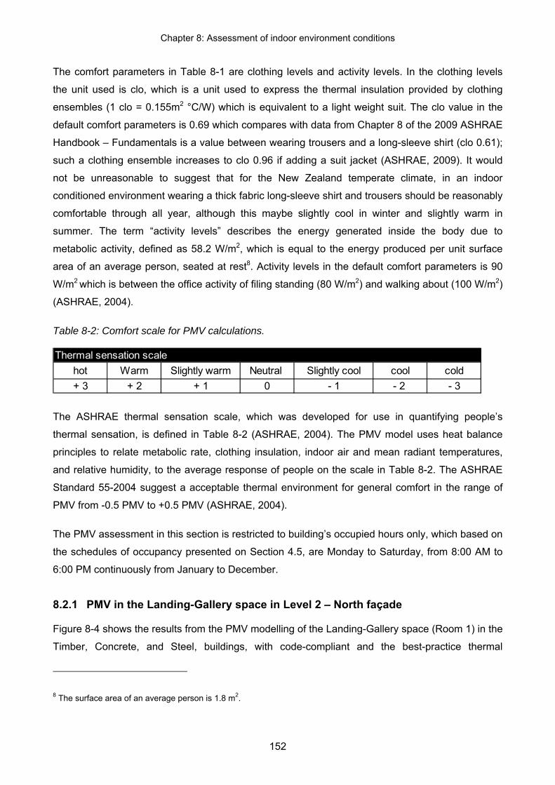
Chapter 8: Assessment of indoor environment conditions
152
The comfort parameters in Table 8-1 are clothing levels and activity levels. In the clothing levels
the unit used is clo, which is a unit used to express the thermal insulation provided by clothing
ensembles (1 clo = 0.155m2 °C/W) which is equivalent to a light weight suit. The clo value in the
default comfort parameters is 0.69 which compares with data from Chapter 8 of the 2009 ASHRAE
Handbook – Fundamentals is a value between wearing trousers and a long-sleeve shirt (clo 0.61);
such a clothing ensemble increases to clo 0.96 if adding a suit jacket (ASHRAE, 2009). It would
not be unreasonable to suggest that for the New Zealand temperate climate, in an indoor
conditioned environment wearing a thick fabric long-sleeve shirt and trousers should be reasonably
comfortable through all year, although this maybe slightly cool in winter and slightly warm in
summer. The term “activity levels” describes the energy generated inside the body due to
metabolic activity, defined as 58.2 W/m2, which is equal to the energy produced per unit surface
area of an average person, seated at rest8. Activity levels in the default comfort parameters is 90
W/m2 which is between the office activity of filing standing (80 W/m2) and walking about (100 W/m2)
(ASHRAE, 2004).
Table 8-2: Comfort scale for PMV calculations.
Thermal sensation scalehot Warm Slightly warm Neutral Slightly cool cool cold+ 3 + 2 + 1 0 - 1 - 2 - 3
The ASHRAE thermal sensation scale, which was developed for use in quantifying people’s
thermal sensation, is defined in Table 8-2 (ASHRAE, 2004). The PMV model uses heat balance
principles to relate metabolic rate, clothing insulation, indoor air and mean radiant temperatures,
and relative humidity, to the average response of people on the scale in Table 8-2. The ASHRAE
Standard 55-2004 suggest a acceptable thermal environment for general comfort in the range of
PMV from -0.5 PMV to +0.5 PMV (ASHRAE, 2004).
The PMV assessment in this section is restricted to building’s occupied hours only, which based on
the schedules of occupancy presented on Section 4.5, are Monday to Saturday, from 8:00 AM to
6:00 PM continuously from January to December.
8.2.1 PMV in the Landing-Gallery space in Level 2 – North façade
Figure 8-4 shows the results from the PMV modelling of the Landing-Gallery space (Room 1) in the
Timber, Concrete, and Steel, buildings, with code-compliant and the best-practice thermal
8 The surface area of an average person is 1.8 m2.

Chapter 8: Assessment of indoor environment conditions
153
envelope. For the best-practice buildings the results of the PMV when convective cooling and
heating operates in the building (commercial HVAC system) has been also included in Figure 8-4.
Timber Concrete Steel Timber - low
Concrete - low
Steel - low
Timber - low
Concrete - low
Steel - low
Eduactional Eduactional Commercial< -0.50 169 140 170 21 6 18 83 54 74-0.50 to 0.50 1609 1895 1776 1086 1222 1157 1427 1625 1571> 0.50 1353 1096 1185 2024 1902 1955 1620 1452 1486
0
500
1000
1500
2000
2500
3000
Hou
rs
Figure 8-4: PMV of Landing-Gallery room in level 2, north facing.
It can be seen in Figure 8-4 that the number of hours within comfortable environmental conditions
is not particularly high in any of the three buildings under any of the three scenarios studied (in
comparison with PMV assessment of the Staff room and Studio 201). The highest number of hours
within comfortable environmental conditions is in the code-compliant buildings (averaged 56% of
the occupied time), followed by the best-practice buildings with the commercial HVAC system
(averaged 50% of the occupied time). Particularly in the best-practice buildings with the
educational HVAC system, the number of hours within comfortable environmental conditions is
very low (average 37% of the occupied time). Almost all of the time in which the buildings are not
within comfortable environmental conditions, occurs when indoor environmental conditions are
slightly warmer to hot (> 0.50 in the scale given in Table 8-2). In the code-compliant buildings, this
environmental condition represents 40% of the time; in the best-practice buildings is 63% and in
the best-practice building with the commercial HVAC system is about 50%.
Figure 8-4 also shows that in all of the three scenarios studied in this research, the Concrete
building has the longest period of time within comfortable environmental conditions, followed by the
Steel building and with the Timber building being the least comfortable. In the code-compliant

Chapter 8: Assessment of indoor environment conditions
154
buildings, the Concrete building has 6% (119 hours) more hours in a comfortable range than the
Steel building and 15% (286 hours) more than in the Timber building. In the best-practice buildings,
the Concrete building has 5% (65 hours) more hours in a comfortable range than the Steel building
and 11% (137 hours) more than in the Timber building. Finally in the best-practice building with the
commercial HVAC system, the Concrete building has 3% (54 hours) more hours in a comfortable
range than the Steel building and 12% (198 hours) than in the Timber building.

Chapter 8: Assessment of indoor environment conditions
155
8.2.2 PMV in Staff room in Level 2 – North façade
The Staff room is the only room in the north side of the building in which there is direct supply of air
from the AHU, and there is cooling in the case of the best practice building with the commercial
HVAC system. Figure 8-5 shows the results from the PMV modelling of this room in the Timber,
Concrete, and Steel, buildings, under the three scenarios studied in this research: code-compliant
buildings, best-practice buildings, and best-practice buildings with the commercial HVAC system.
Timber Concrete Steel Timber - low
Concrete - low
Steel - low
Timber - low
Concrete - low
Steel - low
Eduactional Eduactional Commercial< -0.50 58 39 48 11 0 9 116 101 99-0.50 to 0.50 1862 2047 2002 1525 1687 1563 2163 2394 2358> 0.50 1210 1044 1080 1594 1444 1559 851 636 674
0
500
1000
1500
2000
2500
3000
Hou
rs
Figure 8-5: PMV of Staff room on level 2, north facing.
It can be seen in Figure 8-5 that the amount of hours within comfortable environmental conditions
vary significantly in each of the three different scenarios with the highest amount of hours within
comfortable environmental conditions in the best-practice buildings with the commercial HVAC
system (averaged 56% of the occupied time), followed by the code-compliant buildings (averaged
63% of the occupied time). Consistent with Landing-Gallery space, the best-practice building with
the educational HVAC system have the lowest amount of hours within comfortable environmental
conditions, and in this case, average about 50% of the occupied time. Also similar to the Landing-
Gallery space, most of the time in which the buildings are not within comfortable environmental
conditions, is because indoor environmental conditions are slightly warmer to hot (> 0.50 in the

Chapter 8: Assessment of indoor environment conditions
156
scale given in Table 8-2) but the proportion of time during which these conditions prevail is
significantly reduced compared with the Landing-Gallery space.
Again Figure 8-5 also shows that for this space, in all three scenarios the Concrete building has the
longest period of time within comfortable environmental conditions, followed closely by the Steel
building and with the Timber building being the least comfortable. Generally, the differences
between the hours of slightly warmer to hot conditions in each of the three structural types is not as
great for this space as it was for the landing-gallery.
8.2.3 PMV in Studio room in Level 2 – South façade
For the Studio 201 (Room 3) the corresponding PMV analyses in the Timber, Concrete, and Steel,
buildings, under the three scenarios studied in this research are presented in Figure 8-6.
Timber Concrete Steel Timber - low
Concrete - low
Steel - low
Timber - low
Concrete - low
Steel - low
Eduactional Educational Commercial< -0.50 135 147 143 20 14 18 114 105 126-0.50 to 0.50 2335 2508 2339 2073 2125 2059 2450 2541 2481> 0.50 661 475 649 1038 991 1054 567 485 524
0
500
1000
1500
2000
2500
3000
Hou
rs
Figure 8-6: PMV of Studio 201 on level 2, south facing.
Of the three spaces selected for the PMV analysis, this room (see Figure 8-6) displays the most
acceptable comfort conditions in each of the nine case study buildings (three structural types in
each of the three groups). Although the hours of out-of-comfort conditions are significantly lower -
especially in comparison with the Landing-Gallery – they are still dominantly slight over-heating
rather than under-heating. As in all cases considered here, most of these “over heated” hours are

Chapter 8: Assessment of indoor environment conditions
157
accumulated during the summer period and therefore would be described better as being
conditions of “under-cooling”.
One difference to be noted of Figure 8-6 is that the ranking order in Studio 201 is slightly different
than the ranking order in both of the rooms on the north side of the building. Although in Studio 201
the Concrete building also has the longest period of time within comfortable environmental
conditions in all three scenarios, this is followed more closely by the Steel and the Timber buildings
with the Timber building sometimes more comfortable than the Steel building. In the code-
compliant buildings, the Concrete building has 7% more hours in a comfortable range than the
Steel and the Timber buildings, both having about the same amount of hours in a comfortable
range. In the best-practice buildings, the Concrete building has only 2% more hours in a
comfortable range than the Timber building this time, and 3% than in the Steel building. Finally in
the best-practice buildings with the commercial HVAC system, the Concrete building has 2% more
hours in a comfortable range than the Steel building and 4% than in the Timber building.
8.2.4 Assessment of the Influence of default comfort parameters
In Appendix H an alternative PMV assessment was carried out for the same three rooms in this
section. The conditions for this alternative PMV assessment were basically a reduction of the
clothing levels for the summer months to 0.2 clo (corresponding to sportswear), and an increment
of the same values during winter months to 1 clo (equivalent to wearing trousers, a long-sleeve
shirt, plus a long-sleeve sweater). Activity levels were kept constant to about 70 W/m2 equivalents
to a sedentary work – standing. The results of the variable PMV assessment in Appendix H shows
not a significant variation in the amount of hours within a comfortable environment but significant
reduction of hours in which indoor environmental conditions are slightly warmer to hot, and even a
greater increment of the hours in which the indoor environmental conditions are slightly cool to
cold. In broad terms, in the variable PMV analysis, the average total amount of hours within a
comfortable environment is 13% lower compared with the default PMV analysis. Hours of slightly
cool-to-cold indoor environment are 38% higher in the variable PMV than in the default PMV
analysis. Although the clothing levels were increased during winter conditions in the variable PMV
assessment, the reduction of activity levels (from 90 W/m2 in the default PMV assessment to 70
W/m2 in the variable PMV assessment) have a more significant influence in the outcome of this
assessment with a consequent increase in the amount of hours where environments are slightly
cool-to-cold. Finally, the hours of slightly warm to hot indoor environments are 24% lower in the
variable PMV than in the default PMV analysis. Results in Appendix H are significant because they
suggest that default values are an acceptable generalization to assess comfort conditions, and that
if variations in clothing or in activity levels occur these will have a higher influence in the amount of

Chapter 8: Assessment of indoor environment conditions
158
hours out of comfortable environmental conditions more than changes into the hours within
comfortable environmental conditions.
8.3 Indoor air and surfaces temperature comparison between the Timber, Concrete and Steel buildings:
The aims of this section are:
To study the influence of building’s fabric on indoor environmental conditions;
To identify how building fabric influences the PMV assessment;
To find correlations between building’s fabric and energy assessment.
To achieve these objectives, not only the indoor air temperature but also the surface temperatures
of the buildings constructive elements that have the most significant amount of thermal mass have
been analysed in the Timber, Concrete, and Steel Code-compliant buildings and, in some cases, in
the Low-energy buildings.
The central part of the analysis is to identify a correlation between surface temperatures of
massive structural elements exposed to indoor environments and the resultant air temperature of
the rooms where these massive elements are placed. The focus is on recognizing differences
between the influences on room air temperature of massive structural elements when these are
built using timber (in the Timber building) or concrete (in the Timber, Concrete, and Steel
buildings).
The Structural elements with high quantities of thermal mass were initially identified in Section 4.4;
structural suspended floors, structural shear walls, and stand-alone walls (representation of the
structural columns, beams, and rafters into the BEEM models) were recognized as having the
higher capacitance (C value) of all other construction in the Timber, Concrete, or Steel buildings.
As explained in the introduction to this section (Section 8.1), the detailed indoor temperature
analysis of the Arts building was undertaken in the gallery space as being representative of north-
facing spaces, and in the Studio 201 room as a south-facing representative space. The
temperature analysis in the gallery accounts for both the three storey high space as an entity and
each of the three gallery levels individually.
8.3.1 Whole year, weekly averaged temperature:
A preliminary comparison using weekly average temperatures over a complete year between
indoor air temperatures in the Timber, Concrete and Steel code-compliant buildings with the

Chapter 8: Assessment of indoor environment conditions
159
educational HVAC system, can be seen for the Gallery space (integrated 3 levels air temperature)
in Figure 8-7 and for the Studio 201 room in Figure 8-8.
15
20
25
1 4 7 10 13 16 19 22 25 28 31 34 37 40 43 46 49 52
Tem
pera
ture
(C
)
Main Gallery - 3 levels average
Air _Gallery_Timber Air_Gallery_Concrete Air_Gallery_Steel
Figure 8-7: Main gallery’s three levels weekly averaged temperature across a complete year.
Differences between indoor air temperatures in any of the three different buildings are not
significant when looking at weekly averaged values in any of the two spaces chosen for
temperature differences analysis. In the north facing gallery (Figure 8-7) the highest temperature
difference registered is only 0.4°C between the Steel and the Concrete buildings during the last
week of November (Week 48 in graph); average difference in all cases is also negligible.
A slightly higher peak temperature difference can be seen in the Studio 201 (Figure 8-8) where a
difference of 0.8°C between the Steel and the Concrete building also during the last week of
November (Week 48 in graph) can be seen. Average temperature difference is only 0.3°C between
the Steel and the Concrete building.

Chapter 8: Assessment of indoor environment conditions
160
15
20
25
1 4 7 10 13 16 19 22 25 28 31 34 37 40 43 46 49 52
Tem
pera
ture
(C
)Studio 201
Air _201 Studio_Timber Air_201 Studio_Concrete Air_201 Studio_Steel
Figure 8-8: Studio room on Level 2 (south facing) weekly averaged indoor air temperature across a
complete year.
To obtain a more meaningful comparison between both air temperatures and surface temperatures
of massive structural elements, a much more detailed look into temperature fluctuation needs to be
carried out. Since the comparison between the Timber, Concrete, and Steel buildings in this
research is produced using BEEM software, daily and hourly temperature fluctuations can be
easily obtained.
8.3.2 Hourly temperature comparison – The choice of a winter and a summer representative week
This section shows the detailed indoor air and surfaces temperature analysis in the Timber,
Concrete, and Steel code-compliant and in the best-practice buildings with the educational HVAC
system. The time step for graphical result presentation is hourly and the period of time that will be
analysed will be one week. In such a period of time the detailed dynamics of temperature
fluctuation can be observed in detail. Two separate weeks were chosen for the indoor temperature
analysis in this section: one representative of summer conditions and one of winter conditions. In
Figure 8-9 a graph containing outdoor dry-bulb temperature, direct normal radiation and diffuse
horizontal radiation during the summer representative week (from Monday February 1st until

Chapter 8: Assessment of indoor environment conditions
161
Sunday February the 7th) is shown. In Figure 8-10 the same parameters for the winter
representative week (From Monday June 28th until Sunday 4th of July) are given. Climate data in
Figure 8-9 and Figure 8-10 are taken from the TMY weather file of Nelson. As explained earlier in
Section 4.5.2 climate data in TMY files are typical meteorological values generated from a data
bank much longer than a year in duration, specifically, the climate data in the summer
representative week is from the year 2000, and in the winter representative week is a mixture of
climate data from the years 1997 (June - first three days) and 2006 (July - last four days); see
Table 5-10 for details in TMY climate data sourced.
-15
-10
-5
0
5
10
15
20
25
30
0
200
400
600
800
1000
1200
MO
N
TUE
WE
D
THU
FRI
SAT
SU
N
Tem
pera
ture
(°C
)
W/m
2
Mon 01/Feb to Sun 07/Feb
DirNormRad {W/m2} DifHorzRad {W/m2} DryBulb {C}
Figure 8-9: For a week representative of summer conditions, dry-bulb temperature, direct radiation
and diffuse horizontal radiation are given.
There are no data for total sky cover or opaque sky cover in the TMY file for Nelson. The two
climate characteristics that most significantly influence indoor environmental conditions in buildings
that are available in the TMY weather file are dry-bulb temperature and direct solar radiation
(Duffie & Beckman, 2006). The chosen summer representative week combines days with very low
direct radiation immediately followed by days with very high direct radiation; this is to assess the
response of air and surfaces temperature to clear changes in outdoor environmental conditions.
Particularly on Wednesday February 3rd, peak direct radiation is as low as 219 W/m2 at 7:30 pm
but the previous day (Tuesday February 2nd) records shows a peak direct radiation of 896 W/m2 at

Chapter 8: Assessment of indoor environment conditions
162
10:30 am and on the following day (Thursday February 4th), direct radiation peak to 774 W/m2 at
6:30 pm. Although peak direct solar radiation in the TMY file is recorded on December 26th with
1063 W/m2 at 1:30 pm, peak radiation during the representative summer week is on Sunday
February 7th with 947 W/m2 at 11:00 am, corresponding to a 116 W/m2 (about 10%) lower direct
radiation (intensity) than in the whole year peak.
The most important factor in choosing this particular summer representative week was that, during
this week, changes in direct radiation had a noticeable influence on dry-bulb temperature. It is not
always the case that dry-bulb temperature is responsive to changes in direct or diffuse radiation
but, in the chosen week although daily maximum dry-bulb temperature is mostly constant during
the week, it drops significantly during Wednesday February 3rd with a maximum temperature during
that day of 15°C at 7:00 pm, compared with a peak of 21°C the day before and 22°C the day after.
That drop of temperature during Wednesday February 3rd corresponds to the significant drop of
direct solar radiation. Although peak dry-bulb temperature in the TMY is 27°C on Friday January
15th at 4:00 pm, peak dry-bulb temperature during the summer representative week is 25°C on
Saturday February 6th at 1:00 pm.
-5
0
5
10
15
20
25
30
0
200
400
600
800
1000
1200
MO
N
TUE
WE
D
THU
FRI
SAT
SU
N
Tem
pera
ture
(°C
)
W/m
2
Mon 28/Jun to Sun 04/Jul
DirNormRad {W/m2} DifHorzRad {W/m2} DryBulb {C}
Figure 8-10: For a week representative of winter conditions, Dry-bulb temperature, direct radiation
and diffuse radiation are given.

Chapter 8: Assessment of indoor environment conditions
163
The choice of the winter representative week (from Monday June 28th until Sunday July 4th) follows
roughly the same methodology as that used for the summer representative week, but added to that
is the fact that, included in this week, is the day with the peak annual heating energy consumption
(Monday June 28th) with a peak load of about 167 kW at 8:00 am. Similar to the summer
representative week, Wednesday of this week (June 30th) has a very low direct radiation (peak of
213 W/m2) compared with peak 535 W/m2 the previous day and 787 W/m2 the following day. This
787 W/m2 peak value is about 25% lower than the whole year peak value for direct radiation
intensity.
Unlike the summer representative week, weekly variations on direct radiation have little influence
on dry-bulb temperature during the winter representative week. Daily maximum dry-bulb
temperature remains relatively constant with an average of 11.6°C with a range from maximum
12.4°C on Wednesday June 30th (day with lowest direct radiation) to maximum 9.7°C on Sunday
the July 4th.
8.3.3 Surfaces to be assessed
In the following section, the building’s structural elements chosen for surface temperature analysis
are: structural suspended floors, structural shear walls, and stand-alone walls. As it was initially
explained in Section 4.4, for the purpose of this research the LVL and the concrete structural shear
walls and stand-alone walls are considered to have high thermal mass. Particularly in the case of
the Steel building, no shear walls or stand-alone walls were included in the energy and indoor
space environmental modelling, because these are light-weight elements structured in steel which
is considered to have negligible thermal mass. Only in the suspended floor system of the Steel
building (Comflor ® system), was thermal mass accounted for. As a matter of fact, the Comflor ®
system has a relatively high volume of concrete (0.13 m3/m2), which is greater than the floor
system in the Timber building (Potius ® system 0.08 m3/m2 of concrete) or in the Concrete building
(Interspan ® system with 0.10 m3/m2 of concrete).
Because stand-alone walls are an abstraction of real structural elements such as columns and
beams, they are considered mostly in the way they affect indoor air temperatures. However,
assessing their surface temperature is considered less reliable than the assessment of the surface
temperature of a real building element such as a shear wall or a floor surface. In the Studio 201
room (south-facing), surface temperature is assessed from shear walls and floors, while in the
gallery space (north-facing) surface temperature is assessed in stand-alone walls. This is because
the floor surface is relatively low in that area (mostly void space) and there are no shear walls
available. All graphs include the air temperature of the room/zone in which the particular surface of

Chapter 8: Assessment of indoor environment conditions
164
interest is located to allow the possible influence of thermal mass on indoor air temperature to be
identified.
8.3.4 Gallery temperature analysis – North facing
The north-facing gallery space is particularly interesting, not only because of its exposure to direct
normal radiation (only in Level 2), but also because mechanically supplied air is less influential on
indoor air temperature than in rooms placed in the south side of the building. As it was explained in
Section 4.6.2, the AHU first supplies air to rooms in the south part of the building, and the air
subsequently migrate to rooms in the north part of the building. Because of this, internal gains
produced in rooms on the south increases the temperature of the air before it arrives in rooms in
the north, in particular to the gallery space. Because of this, a smaller temperature difference exists
between the mechanically supplied air and indoor air temperature in north facing spaces.
8.3.4.1 Level 2 Gallery – Detailed temperature analysis
10
15
20
25
30
MO
N
TUE
WE
D
THU
FRI
SAT
SU
N
Tem
pera
ture
(°C
)
Air_Gallery Level 2_T Surface_Stand-alone wall Level 2_TAir_Gallery Level 2_C Surface_Stand-alone wall Level 2_C
Figure 8-11: Summer representative week: Level 2 Gallery, stand-alone walls surface
temperatures in the code-compliant Timber (_T) and Concrete (_C) buildings.
Stand-alone wall surface temperatures, together with room air temperature in Level 2 of the Gallery
space of the Timber and Concrete code-compliant buildings during the summer representative
week can be seen in Figure 8-11; and Figure 8-12 is the equivalent for the winter representative
week. Level 2 is the only level in the gallery that does receive direct solar radiation, particularly in

Chapter 8: Assessment of indoor environment conditions
165
winter. As can be seen in the Arts building cross-sections on Figure 4-2, Section 4.1.2 on the north
side of Level 3 the influence of a relatively large roof overhang blocks the direct sunlight on Level 3
during the whole year and on Level 2 during summer.
10
15
20
25
30
MO
N
TUE
WE
D
THU
FRI
SAT
SU
N
Tem
pera
ture
(°C
)
Air_Gallery Level 2_T Surface_Stand-alone wall Level 2_TAir_Gallery Level 2_C Surface_Stand-alone wall Level 2_C
Figure 8-12: Winter representative week: Level 2 Gallery, stand-alone walls surface temperatures
in the code-compliant Timber (_T) and Concrete (_C) buildings.
Relevant observations relating to Figure 8-11 and Figure 8-12 are:
In the summer representative week, the timber stand-alone surface temperature has a daily
fluctuation similar to that of the air temperature and essentially in phase. Generally the
timber surface temperature is offset above the air temperature by about one degree.
The concrete surface temperature displays a much smaller amplitude, demonstrating the
energy-buffering characteristics due to the higher thermal capacity of this material.
There is no strong evidence of significant phase difference – either leading or lagging –
between the concrete surface temperature and the corresponding air temperature. During
the summer, however, there is very limited solar gain directly to the concrete surface so the
surface energy balance is dominated by convective heat exchange.
Although the effect of direct normal radiation on the surface of the timber and concrete stand
alone wall shows a radical increment of surface temperatures in both the timber and the
concrete surface, the surface’s temperature of the timber stand-alone wall increases to a
much higher temperature than in the concrete surface.

Chapter 8: Assessment of indoor environment conditions
166
Peak surface temperatures for the concrete wall remain cooler than air temperature but, in
the Timber building, the surface temperature of the timber wall is much higher than the air
temperature in that building.
There is a variation of about 1°C higher during daily peak air temperature in the Timber
building compared with the Concrete building and during the night temperature in the Timber
building drops also about 1°C below the Concrete building air temperature.
In the timber stand-alone wall: Without direct normal radiation, the timber surface temperature has
a daily fluctuation similar to that of the air temperature, normally being higher by less than 1°C.
With exposure to direct normal radiation, however, the timber surface’s temperature increases to a
much higher temperature than the air temperature.
In the concrete stand-alone wall: Without direct normal radiation, the concrete surface responds
more slowly than air temperature, and does not normally increases above air temperature. With
direct radiation exposure, surface temperature variation during day and night is higher but still
lower than air temperature. Peak surface temperature is also lower than air temperature.
These observations are consistent with the characteristics of these wall materials: Compared with
the concrete stand-alone wall, the timber stand-alone wall has relatively little capacity to buffer
some of the heat/energy when direct radiation is available, but seems to be a relatively good heat
buffer when the incident radiation intensity is much lower.

Chapter 8: Assessment of indoor environment conditions
167
8.3.4.2 Level 1 and Level 3 Gallery – Air and surfaces temperatures
Stand-alone wall surface temperatures, together with room air temperature in Level 1and on Level
3 of the Gallery space for Timber and Concrete code-compliant and best-practice buildings, can be
seen during the summer representative week in Figure 8-13, and during the winter representative
week in Figure 8-14.
15
20
25
30
MO
N
TUE
WE
D
THU
FRI
SAT
SU
N
Tem
pera
ture
(°C
)
Gallery on Level 1 - Air + Surface temp. (Summer)
Air_Gallery Level 1_T Surface_Stand-alone wall Level 1_T
Air_Gallery Level 1_C Surface_Stand-alone wall Level 1_C (a)
15
20
25
30
MO
N
TUE
WE
D
THU
FRI
SAT
SU
N
Low - Gallery on Level 1 - Air + Surface temp. (Summer)
Air_Gallery Level 1_T Surface_Stand-alone wall Level 1_TAir_Gallery Level 1_C Surface_Stand-alone wall Level 1_C (b)
15
20
25
30
MO
N
TUE
WE
D
THU
FRI
SAT
SU
N
Tem
pera
ture
(°C
)
Gallery on Level 3 - Air + Surface temp. (Summer)
Air_Gallery Level 3_T Surface_Stand-alone wall Level 3_T
Air_Gallery Level 3_C Surface_Stand-alone wall Level 3_C (c)
15
20
25
30
MO
N
TUE
WED TH
U
FRI
SAT
SUN
Low - Gallery on Level 3 - Air + Surface temp. (Summer)
Air_Gallery Level 3_T Surface_Stand-alone wall Level 3_T
Air_Gallery Level 3_C Surface_Stand-alone wall Level 3_C (d)
Figure 8-13: Stand-alone wall surface temperatures and indoor air temperatures during the
summer representative week – On Level 1 of the code-compliant (graph (a)) and best-practice
(graph (b)) Timber and Concrete buildings, and on Level 3 of the code-compliant (graph (c)) and
best-practice (graph (d)) Timber and Concrete buildings.

Chapter 8: Assessment of indoor environment conditions
168
10
15
20
25M
ON
TUE
WE
D
THU
FRI
SAT
SU
N
Tem
pera
ture
(°C
)
Gallery on Level 1 - Air + Surface temp. (Winter)
Air_Gallery Level 1_T Surface_Stand-alone wall Level 1_TAir_Gallery Level 1_C Surface_Stand-alone wall Level 1_C (a)
10
15
20
25
MO
N
TUE
WE
D
THU
FRI
SAT
SU
N
Low - Gallery on Level 1 - Air + Surface temp. (Winter)
Air_Gallery Level 1_T Air_Gallery Level 1_C
Surface_Stand-alone wall Level 1_C Surface_Stand-alone wall Level 1_T (b)
10
15
20
25
30
MO
N
TUE
WE
D
THU
FRI
SAT
SU
N
Tem
pera
ture
(°C
)
Gallery on Level 3 - Air + Surface temp. (Winter)
Air_Gallery Level 3_T Surface_Stand-alone wall Level 3_T
Air_Gallery Level 3_C Surface_Stand-alone wall Level 3_C (c)
10
15
20
25
30
MO
N
TUE
WED TH
U
FRI
SAT
SUN
Low - Gallery on Level 3 - Air + Surface temp. (Winter)
Air_Gallery Level 3_T Surface_Stand-alone wall Level 3_T
Air_Gallery Level 3_C Surface_Stand-alone wall Level 3_C (d)
Figure 8-14: Stand-alone wall surface temperatures and indoor air temperatures during the winter
representative week – On Level 1 of the code-compliant (graph (a)) and best-practice (graph (b))
Timber and Concrete buildings, and on Level 3 of the code-compliant (graph (c)) and best-practice
(graph (d)) Timber and Concrete buildings.
Relevant observations relating to Figure 8-13 and Figure 8-14 are:
On Level 1, the surface temperatures of the timber and concrete stand-alone wall are
similar, and these are higher than their respective indoor air temperatures.
On Level 3 the surface temperature of the concrete stand-alone wall does not swing
significantly between day and night. In contrast, the surface temperature on the timber
stand-alone wall vary significantly between day and night and is similar (slightly higher) than
the indoor air temperature.
Gallery’s Level 1 air temperature is very similar in the Timber and Concrete buildings during
the day and is slightly lower in the Timber building during the night (about 1°C lower).

Chapter 8: Assessment of indoor environment conditions
169
In both Figure 8-13 and Figure 8-14 the daily air and surface temperature peaks in the code-
compliant buildings are slightly lower than in the best-practice buildings. During the night,
both air and surface temperatures drop significantly lower in the code-compliant building
compared with the best-practice building. In the best-practice case, air and surface
temperatures in the Timber building are lower than in the Concrete building. This is
consistent in the Studio 201 and in all three levels of the Gallery. The effect of increasing
insulation values in the thermal envelope is an increment of both lowest and highest indoor
air temperature during summer and only lowest indoor temperatures during winter.
8.3.5 Studio 201 surface and air temperature analysis – South facing
8.3.5.1 Studio 210 - Shear walls
Shear wall surface temperatures, together with room air temperature in the Studio 201 for the
Timber and Concrete code-compliant buildings, can be seen during the summer representative
week in Figure 8-15 and during the winter representative week in Figure 8-16. Because Studio 201
is facing south, there is no direct normal radiation influencing indoor environmental conditions,
resulting in outdoor dry-bulb temperature being a stronger influence than in the north façade.
10
15
20
25
30
MO
N
TUE
WE
D
THU
FRI
SAT
SU
N
Tem
pera
ture
(°C
)
Air_Studio RM 201_T Surface_Shear wall East & West RM 201_TAir_Studio RM 201_C Surface_Shear wall East & West RM 201_C
Figure 8-15:– Shear wall surface temperature in the code-compliant Timber and Concrete buildings
during the summer representative week.

Chapter 8: Assessment of indoor environment conditions
170
10
15
20
25
30
MO
N
TUE
WE
D
THU
FRI
SAT
SU
N
Tem
pera
ture
(°C
)
Air_Studio RM 201_T Surface_Shear wall East & West_RM 201_TAir_Studio RM 201_C Surface_Shear wall East & West_RM 201_C
Figure 8-16: Shear wall surface temperatures in the code-compliant Timber and Concrete buildings
during the winter representative week.
From Figure 8-15 and Figure 8-16, relevant observations are:
Indoor air temperature is very similar in the Timber and Concrete buildings; especially during
the summer representative week. During winter, indoor air temperature in the Timber
building drops during the night significantly more than in the Concrete building.
During the summer representative week, surface temperatures in shear walls are higher
than indoor air temperature, but this is reversed during the winter representative week.
Surface temperature in the timber shear wall is higher and much closer to indoor air
temperature (higher in winter, lower in summer) than surface temperature in the concrete
shear wall. In the concrete shear wall, surface temperature is higher than indoor air
temperature during unoccupied hours and lower than indoor air temperature during
occupied hours.
Due to a higher capacitance in the concrete shear wall, changes in surface temperature occur
more slowly than in the timber shear wall. Furthermore, the surface temperature does not peak in
the concrete shear wall as high as it does in the timber shear wall. Summer, surface temperature in
shear walls is higher than indoor air temperature, but in winter, surface temperature is lower than
indoor air temperature. Although there is forced convection due to higher air velocity, the heat
transfer between air and materials is not particularly high, or at least not high enough to

Chapter 8: Assessment of indoor environment conditions
171
significantly influence indoor air temperature. Higher heat transfer can be seen more clearly in
rooms facing north where direct radiation is incident on wall surfaces.
Incidentally, there is evidence in Figure 8-16 that the as-modelled heating system did indeed have
sufficient heating capacity to achieve the set-point temperature of 22°C (remembering that this set-
point had an associated dead band of 2 K). Referring back to the earlier discussion (Section 6.5)
on the apparent shortfall (compared with monitored values), this means that the third explanation
offered there is not valid. Hence it must be some combination of the other possible explanation
which contributes to the lower weekly average temperatures, but there is insufficient evidence to
identify which one or ones it might be.
8.3.5.2 Studio 201 – Floor surface temperature
15
20
25
30
MO
N
TUE
WED
THU
FRI
SAT
SUN
Tem
pera
ture
(°C
)
Studio 201 - Floor temp. (Summer)
Air_Studio RM 201_T Air_Studio RM 201_CAir_Studio RM 201_S Surface_Floor RM 201_TSurface_Floor RM 201_C Surface_Floor RM 201_S (a)
15
20
25
30M
ON
TUE
WED
THU
FRI
SAT
SUN
Low - Studio 201 - Floor temp. (Summer)
Air_Studio RM 201_T Air_Studio RM 201_CSurface_Floor RM 201_T Surface_Floor RM 201_CSurface_Floor RM 201_S Air_Studio RM 201_S (b)
10
15
20
25
MO
N
TUE
WED
THU
FRI
SAT
SU
N
Tem
pera
ture
(°C
)
Studio 201 - Floor temp. (Winter)
Air_Studio RM 201_T Air_Studio RM 201_C
Air_Studio RM 201_S Surface_Floor RM 201_T
Surface_Floor RM 201_C Surface_Floor RM 201_S (c)
10
15
20
25
MO
N
TUE
WED TH
U
FRI
SAT
SUN
Low - Studio 201 - Floor temp. (Winter)
Air_Studio RM 201_T Surface_Floor RM 201_TAir_Studio RM 201_C Surface_Floor RM 201_CAir_Studio RM 201_S Surface_Floor RM 201_S (d)
Figure 8-17: On Studio 201, floor surface’s and indoor air temperature - During the summer
representative week in the code-compliant (a) and best-practice (b) buildings, and during the winter
representative week in the code-compliant (c) and best-practice (d) buildings.

Chapter 8: Assessment of indoor environment conditions
172
In Figure 8-17 the floor surface temperatures and room air temperature can be seen during the
same summer and winter representative weeks in the Studio 201 for the Timber, Concrete, and
Steel code-compliant and best-practice buildings9.
Specific comments related to plots on Figure 8-17 are:
The most significant differences of indoor air and surfaces temperature in the code-
compliant and the best-practice buildings are; a milder temperature swing during day and
night with an average increase of temperatures particularly during summer. During winter,
minimum temperatures are higher in the best-practice building but peak temperatures during
the day are similar.
Compared with shear walls surface temperatures, floor surface temperatures are very
similar in the all three buildings in both thermal envelope scenarios. All three floor systems
are composite floors: concrete-timber (Timber and Concrete building) and concrete-steel
(Steel building), having a concrete surface exposed to the interior space having a thickness
ranging from 75 mm in the Concrete and Timber building, to about 150mm in the Steel
building. This common factor of the surface material being concrete has resulted in
similarities in surface temperature.
The indoor air temperature in the Steel building is very similar to that in the Timber and
Concrete building during summer. Differences are more evident during the winter
representative week where night time indoor air temperature of the Timber building drops
further compared with temperatures in the Concrete and in the Steel buildings.
9 In the graphs in Figure 8-17, temperature range in the left side vertical axis, during summer representative week (15°C
to 30°C) is different than the temperature range during winter representative week (10°C to 25°C), this is to keep in the
graph a 15°C temperature scale suitable for the analysis of relatively small temperature differences in such a small
graphs.
Chapter 8: Assessment of indoor environment conditions
173
8.4 Discussion of indoor environmental conditions
8.4.1 PMV assessment - final discussion
Looking at the results using a default PMV assessment, in all three rooms analysed in this section
most of the time in which the buildings are not within comfortable environmental conditions, is
because indoor environmental conditions are slightly warmer to hot (> 0.50). There is, however, a
small amount of hours in all three rooms, but mostly in the code-compliant buildings and in the
best-practice buildings with the commercial HVAC system, where the indoor environmental
conditions are slightly cool to cold (<-0.5 in the scale given in Table 8-2). The amount of hours in
this category is quite similar in the Landing-Gallery and in the Studio 201 and slightly lower in the
Staff room. There are essentially no slightly cool-to-cold hours in the best-practice buildings.
In the Landing-Gallery the time within comfortable environmental conditions is the lowest of any of
the rooms in which PMV assessment was carried out. In all three scenarios, it is in the code-
compliant buildings where the highest amount of time with comfortable environmental conditions
exist; this is followed by the best-practice building with the commercial HVAC system, where the
hours within comfortable environmental conditions is almost equivalent to the hours with slightly
warm-to-hot environmental conditions. The best-practice buildings exhibit the undesirable
characteristic that the hours with slightly warm-to-hot environmental conditions are considerably
higher than the hours within comfortable indoor environment. Although differences are not
significant, the Concrete building is always the most comfortable, and Timber the least. In fact it is
only in the code-compliant scenario, that the landing-gallery in the Timber building has more hours
with a comfortable environment than hours in a slightly warm to hot indoor environment.
In the Staff room, from all three scenarios, it is the best-practice buildings with the commercial
HVAC system which exhibit the highest amount of hours with comfortable environmental conditions
followed by the code-compliant buildings. In the best-practice buildings, the hours within
comfortable environmental conditions are almost equivalent to the hours with slightly warm to hot
environmental conditions. More specifically, time with slightly warm to hot environmental conditions
is higher in the Timber building, equivalent in the Steel building, and lower in the Concrete building
than the time within comfortable indoor environment. Although differences between indoor
environmental conditions between the Timber, Concrete, and Steel buildings are more marked
than in the Landing-Gallery space, these are still not significant. In this room, the Concrete building
is always the most comfortable followed closely by the Steel building and with the Timber more
clearly in a lower position.

Chapter 8: Assessment of indoor environment conditions
174
For the Studio 201; the third and final space subjected to PMV analysis, the hours within
comfortable environmental conditions is the highest of the three rooms. Although it is the best-
practice buildings with the commercial HVAC system where the amount of time with comfortable
environmental conditions is the highest, this is very similar to the code-compliant buildings. The
main difference is that in the best-practice buildings with the commercial HVAC system the Timber,
Concrete, and Steel buildings have very similar hours with comfortable environmental conditions
while in the code-compliant buildings these hours are higher in the Concrete building followed by
the Steel and the Timber with almost the same outcome. The best-practice buildings have the least
time with comfortable environmental conditions but the number of these hours is still very high
compared with hours with slightly warm to hot environmental conditions. Although differences are
not significant, the Concrete building is always the most comfortable, followed by the Steel and the
Timber with very similar outcomes.
It is worth noting again that the modelling of the indoor temperatures in T-block appeared to over-
estimate the diurnal swing but that this seemed to have had a minimal impact on the broad
agreement between the modelled and monitored values for the operational energy usage for this
building. In making that observation (in Section 5.6.3) it was remarked that an overestimate of
diurnal swing would not necessarily result in the model predicting fewer hours of desirable thermal
comfort conditions either, because the model’s low estimate of the daily temperature minima would
occur outside the occupied hours during which thermal comfort was of importance.
This reasoning is mentioned here because if, for the Arts building (the primary focus of this
research), the diurnal swing is also being overestimated in the modelling of some of the spaces,
the PMV analysis – which was totally based on modelled temperatures – would conclude that for
some hours the perceived thermal comfort was outside the accepted comfort range whereas, in
reality, those same hours might lie within the comfort range. If this argument is accepted, the
consequences would be that for all of the building case studies in this research, it is probable that
the number of hours in which thermal comfort has been determined (from PMV analysis) as being
over-cool or over-hot are higher than they would be in the actual building. In other words, the
assessments of likely perceived thermal comfort within any of the buildings that were modelled is
likely to be a little pessimistic.
8.4.2 Surface and air temperatures - Discussion
Surfaces and air temperatures were analysed in two rooms: on the Landing-Gallery, facing north
and therefore frequently exposed to direct solar radiation, and on the Studio 201, facing south. As
a consequence, in rooms facing north the mechanisms of heat transfer between the surrounding
environment and the materials includes both radiation and convection. In rooms facing south the
Chapter 8: Assessment of indoor environment conditions
175
mechanism of heat transfer between the surrounding environment and the materials is dominated
by convection.
When radiation is the dominant heat transfer mechanism, higher heat transfer can be seen more
clearly. Because the timber wall has much lower capacity to buffer heat than a concrete wall, the
surface temperature in timber increases to a much higher temperature than for concrete surfaces.
Peak surface temperature in the timber wall is much higher than indoor air temperature. On a
concrete wall, the maximum surface temperature increases to a lower temperature than air
temperature. The concrete wall surface temperature responds more slowly than both the timber
wall surface temperature and the air temperature.
When convection is the dominant heat transfer mechanism, a lower heat transfer can be seen, and
the capacity to buffer heat is similar in the timber and concrete walls. Still, the surface temperature
of the timber walls is higher than in the concrete wall and has a daily fluctuation similar to the air
temperature (normally higher temperature but by less than a degree across the day). Surface
temperature on the concrete walls responds to daily temperature fluctuation more slowly than air
temperature, and is lower than indoor air temperature during occupied hours (conditioned) and
higher during unoccupied hours (unconditioned).
As a result of space pre-conditioned mechanically supplied air, indoor air temperature during
summer in the Concrete building is very similar to that in the Timber and Steel buildings
(Compared with the Concrete building, the Timber building indoor air temperature is about 1°C
higher during the day and 1°C lower during the night). During winter conditions on the other hand,
night time indoor air temperature of the Timber building drops significantly lower than in the
Concrete and in the Steel buildings. The forced convection that should occur because of the high
indoor air velocity in rooms with mechanical ventilation appears not to increase significantly the
heat transfer between air and materials which appears to be insufficient to significantly influence
indoor air temperature.
Lower heat loss through the thermal envelope reduces diurnal temperature swing with an average
increase of indoor temperatures, particularly during summer. It also increases the maximum air
and surface temperatures during the day, and during the night higher lower temperatures occur.
The effect of increasing insulation values in the thermal envelope produces an increase of both
minimum and maximum indoor air temperature during summer, but only minimum indoor
temperatures during winter. During winter, minimum temperatures are higher in the best-practice
building but peak temperatures during the day are similar to those in the code-compliant buildings.

Chapter 9: Improvement of energy performance and comfort conditions
176
9 Improvement of energy performance and comfort conditions
This chapter describes possible improvement of the energy performance and comfort conditions of
the Arts Timber building by using three possible methods of improving overall indoor comfort
conditions and subsequently reducing space conditioning energy consumption. These three
methods are night-time ventilation, exterior louvres, and the use of Phase-Change-Materials
(PCM).
9.1 Night-time ventilation and solar shading system replacement
This chapter analyses alternatives scenarios to achieve a reduction of space conditioning energy
consumption, while at the same time improving indoor environmental conditions of the best-
practice buildings with a commercial HVAC system. This building group represents the buildings in
which the thermal envelope has been upgraded to a New Zealand best-practice standard, and at
the same time these buildings are modelled using HVAC systems that include cooling and in which
heating and cooling systems in place have a high performance for a relatively low energy
consumption. As it was established initially in Section 4.6.2, to assess the effect that night-time
ventilation has on the influence of thermal mass on cooling energy consumption and indoor
comfort conditions, this section compares energy and PMV results of the best-practice buildings
with commercial HVAC system, with and without night-time ventilation. The schedule and
conditions of operation can be seen in Section 4.6.2; in the commercial HVAC system without
night-time ventilation, the AHU operates during week days (including Saturday) from 8:00 am until
6:00 pm (see Section 4.5.3 for more details).
9.1.1 Louvres
In Section 4.1.2 where a cross-section of the actual Arts building was shown, a relatively large
overhang can be seen as an extension of the roof on the north side of Level 3. The overhang is
designed such that on Level 3, no direct solar radiation can reach the interior space year round,
and on Level 2 direct solar radiation is available in interior spaces during winter only from March
until September, but more significantly during May -July, when the solar altitude angle is below 45°.
No windows facing north are available in Level 1, but the gallery in that level gets diffuse natural
light from Level 2 and 3. This is because in the actual Arts building there is an unmodelled
construction attached the north side of Level 1.
A better control of the transmission of direct solar radiation into indoor environments can improve
indoor environmental conditions and, possibly, reduce conditioning energy in the Arts building

Chapter 9: Improvement of energy performance and comfort conditions
177
(Timber) and in its alternatives in Concrete and Steel. External louvres are an appropriate
alternative to achieve this and can be easily modelled using the BEEM software of choice in this
research (VE). The overhang was replaced by louvres placed over the glazed area on the north
side of Level 2 and 3. The approach taken for the modelling of louvres in VE was by making them
control the transmission of solar radiation, homogeneously across the glazed area. Table 9-1
shows the factors for controlling transmission of solar radiation by the louvres modelled in VE. It
can be seen that just above a solar angle of 60° the louvres start reducing the solar radiation
transmission by 50% and over an angle of 75° transmission is reduced to 0%. Louvres were
modelled in the best-practice buildings using the commercial HVAC system, basically to see the
impact of them on not only heating energy but also on cooling energy.
Table 9-1: Solar radiation transmission factor for louvres.
Transmission factor at 15° increment (values in range 0.0 - 1.0 )0° 15° 30° 45° 60° 75° 90°
0.00 0.00 0.00 0.00 0.50 1.00 1.00
9.2 Results on energy consumption
Timber Concrete Steel Timber Concrete Steel Timber Concrete SteelCommercial Commercial (No night-vent.) Commercial (Louvres)
Heating (Comb.) 33.1 32.0 32.7 33.0 31.7 32.5 37.3 38.0 37.9Chillers (Elec.) 3.8 3.2 3.8 5.2 4.9 5.4 3.3 2.9 3.3Fans (Elec.) 9.5 9.3 9.3 6.9 6.5 6.5 10.4 10.2 10.2Total (Comb.) 46.4 44.5 45.8 45.1 43.2 44.4 50.9 51.1 51.4
0
10
20
30
40
50
60
MW
h
Figure 9-1: Energy consumption in all cases compared in this section.

Chapter 9: Improvement of energy performance and comfort conditions
178
In Figure 9-1, the space conditioning energy consumption information of the best-practice buildings
with the commercial HVAC system (commercial), is compared against the same set of case study
buildings and HVAC system but without night-time ventilation (“No night- vent.”), and the same set
of case study buildings and HVAC system (with night-time ventilation) but with louvres instead of
the actual overhang.
Total conditioned energy consumption is very similar in the commercial buildings (average of 45.6
MWh/yr) and in the buildings with no night-time ventilation (average of 44 MWh/yr), but higher in
the buildings with louvres (average 51 MWh/yr). The increment of total conditioning energy
consumption in the buildings with louvres when compared to the commercial buildings is mostly in
heating energy (about 15% higher) and, less significantly, in fan energy consumption (average is
9% higher). Chiller energy is actually lower (about 12%) in the buildings with louvres than in the
commercial buildings. Slightly lower total space conditioning energy in the buildings with no night-
time ventilation compared with the commercial buildings is, for obvious reasons, in fans energy
(about 30% lower); chiller energy on the other hand is larger in the buildings without night-time
ventilation.
Differences in total space conditioning energy consumption between building construction types
(Timber, Concrete, and Steel) are insignificant in buildings with louvres (1% difference between the
highest (Concrete) and the lowest (Timber) space conditioning energy consumer). The proportional
difference of the space conditioning energy consumption between each building construction type
is the same in the commercial buildings and in buildings with no night-time ventilation (a 4%
difference between the highest (Timber) and the lowest (Concrete) space conditioning energy
consumption).
There is a reduction of heating energy consumption together with an increment of chiller energy
consumption in the building with no night-time ventilation compared with commercial buildings. In
those cases, although differences are not significant (+- 1MWh/year), with the timber building
having lower heating demand and higher cooling demand than the concrete building.
9.3 Results of PMV assessment
9.3.1 PMV of the Landing-Gallery space – North façade
Figure 9-2 shows the results from the PMV assessment of the Landing-Gallery space in the best-
practice buildings with the commercial HVAC system (commercial), is compared against the same
set of case study buildings and HVAC system but without night-time ventilation (“No night-vent.),

Chapter 9: Improvement of energy performance and comfort conditions
179
and the same set of case study buildings and HVAC system (with night-time ventilation) but with
louvres instead of the actual overhang (”Louvres”).
The amount of hours within a comfortable indoor environment in the buildings with louvres (73% of
the time) is significantly higher than in the commercial buildings (about 50% of the time), and in the
buildings with no night-time ventilation (40% of the time). This is mainly because of the reduction of
hours in warm-to-hot environments which represent a 20 % in the buildings with louvers, a 50% in
the commercial buildings and a 60 % in the buildings with no night-time ventilation. Time within
cool-to-cold environments is low across all cases, ranging from 8% in the buildings with louvres to
1% in the buildings with no night-time ventilation (2% in commercial buildings).
Timber Concrete Steel Timber Concrete Steel Timber Concrete SteelCommercial Commercial (No night-vent.) Commercial (Louvres)
< -0.50 83 54 74 29 11 22 256 242 268-0.50 to 0.50 1427 1625 1571 1156 1283 1246 2256 2336 2288> 0.50 1620 1452 1486 1946 1837 1863 619 553 574
0
500
1000
1500
2000
2500
3000
Hou
rs
Figure 9-2: Landing gallery on level 2 north orientation – PMV comparison of the commercial
building with two variations.
9.3.2 PMV in Staff room Level 2 – North façade
The Staff room is the only room in the north side of the building in which there is direct supply of air
from the AHU, and there is cooling in the case of the best-practice building with the commercial
HVAC system. Figure 9-3 shows the results from the PMV assessment of the Staff Room in the
commercial buildings, compared against the buildings with no night-time ventilation, and the
buildings with louvres.

Chapter 9: Improvement of energy performance and comfort conditions
180
The overall results of the PMV assessment in the Staff Room in all three building groups follow the
same pattern as in the Landing-Gallery space, but with an increment of hours within comfortable
conditions across all building groups. Again, the amount of hours within a comfortable environment
is the highest in the building with louvres (84%) followed by the commercial building (74%) and the
buildings without night-time ventilation (64%). Hours of warm-to-hot environmental conditions are
very low in the buildings with louvres (9%) and relatively high in buildings with no night-time
ventilation (36%) with the commercial buildings in between (23%). Again, the amount of hours
within cool-to-cold environments is very low – negligible.
Timber Concrete Steel Timber Concrete Steel Timber Concrete SteelCommercial Commercial (No night-vent.) Commercial (Louvres)
< -0.50 116 101 99 5 0 1 226 219 223-0.50 to 0.50 2163 2394 2358 1916 2073 2009 2577 2656 2616> 0.50 851 636 674 1209 1058 1121 328 256 292
0
500
1000
1500
2000
2500
3000
Hou
rs
Figure 9-3: Staff room on level 2 north orientation – PMV comparison of the commercial building
with two variations.
Differences in the PMV assessment between building construction types (Timber, Concrete, and
Steel) of spaces on the north façade of the arts building are not significant. It can be said that the
amount of hours within comfortable environmental conditions is always (but not significantly) higher
in the Concrete building, and lower in the Timber building (average difference of 5% of the
occupied time across all scenarios).

Chapter 9: Improvement of energy performance and comfort conditions
181
9.3.3 PMV in Studio room in Level 2 – South façade
Figure 9-4 shows the results from the PMV assessment of the Studio 201 (South façade) in the
commercial buildings, the buildings with no night-time ventilation, and in the buildings with louvres.
The pattern presented in the results of the PMV assessment of the Studio 201 (south façade) is
different from the pattern of results in the Landing-Gallery space and in the Staff room, which are
both on the north façade. Both the commercial building and the buildings with louvres have
practically the same PMV results, with relatively high amount of hours within comfortable
conditions (about 80%), with only 17% of the occupied hours within warm-to-hot environment, and
a low 4% of occupied hours within cool-to-cold hours. In the buildings with no night-time ventilation,
the amount of occupied hours within warm-to-hot environment increases significantly to 36%
reducing the amount of hours within comfortable conditions to 70%. Hours of cold-to-cold
environment in that building are practically nonexistent.
Timber Concrete Steel Timber Concrete Steel Timber Concrete SteelCommercial Commercial (No night-vent.) Commercial (Louvres)
< -0.50 114 105 126 26 12 29 124 120 138-0.50 to 0.50 2450 2541 2481 2140 2178 2131 2445 2536 2478> 0.50 567 485 524 965 941 970 561 475 515
0
500
1000
1500
2000
2500
3000
Hou
rs
Figure 9-4: Studio room 201 on level 2 south orientation – PMV comparison of the commercial
building with two variations.
Differences between building constructions types (Timber, Concrete, or Steel) are even lower than
in rooms on the north façade of the building. Again the Concrete buildings spend some more hours
within a comfortable environment by reducing the hours of warm-to-hot environment.

Chapter 9: Improvement of energy performance and comfort conditions
182
9.3.4 Discussion on improvement of energy performance and comfort conditions
The replacement of the overhang by louvres has a large impact into improving comfort conditions
in rooms facing north, increasing the amount of hours within comfortable conditions by about 30%.
Improvement to comfort conditions comes with an energy penalty, however, with a 12% increment
of annual space conditioning energy consumption (Although cooling energy is reduced by 12%,
heating energy consumption is 16% higher with proportionally a much larger energy consumption
than cooling).
Overheating is the main reason for discomfort in the commercial buildings. By reducing the
transmission of high solar radiation into the building (for a sun angle above 60° the louvres start to
reduce direct radiation transmission) overheating is reduced but an increment on heating energy is
required. The presence of louvres also tempers the difference in comfort conditions between
buildings constructions types. On the other hand, the increment of the transmission of direct solar
radiation makes differences more significant. These analyses, and the conclusions drawn from
them, are for the situation of the louvres being installed with a fixed angle. Louvres having a
variable tilt angle (either motorised, or seasonally adjustable) are a means of reducing unwanted
solar gains at times of the year or times of day when overheating would occur, but admitting solar
gains when it would be energy-beneficial to do so.
When there is no night-time ventilation the amount of hours of warm-to-hot environments increases
but proportional differences between buildings construction types remain very similar. This
reduction in hours within comfortable environmental conditions in buildings with no night-time
ventilation implies less space conditioning energy consumption in those buildings, mostly because
of the reduction in fan energy consumption, although there is an increment on chiller energy
consumption.
Although not significantly, in all three scenarios the Concrete building has the higher amount of
hours within comfortable environment and the lower space conditioning energy, followed by the
Steel and the Timber buildings. These differences are negligible when louvres are used instead of
the overhang.
9.4 Improvement of the energy performance and comfort conditions of the Timber building – use of PCM
9.4.1 PCM materials - Introduction
An alternative to improve the thermal capacity of light-weight buildings is the use of phase change
materials (PCM). PCM materials not only absorb sensible heat as the indoor temperature

Chapter 9: Improvement of energy performance and comfort conditions
183
increases but also absorb latent heat when melting, and release the stored heat when freezing,
both at an almost constant temperature. PCM can be used in buildings to significantly improve the
thermal mass as they have a much greater ability to store heat than conventional building materials
such as concrete. Concrete has a sensible heat storage capacity of 1.0 kJ/kgK, whereas an
inorganic phase change material such as calcium chloride hexahydrate can store up to 193 kJ/kg
during phase transition (Ip, Dyball, & Miller, 2008).
A significant development in phase change technology is the ability to microencapsulate PCMs.
Microencapsulation is the packaging of micron-sized PCM materials (both liquids and solids) in the
form of capsules, ranging from less than 1μm to more than 300μm. Microencapsulated PCMs can
be used to introduce high thermal storage capacity into conventional building materials such as
gypsum plaster, concrete, and plasterboard (Ip, et al., 2008).
In this section, a modelling exercise to illustrate the effect of PCM into indoor environmental
conditions of the actual Arts building (Timber buildings) was carried out. The PCM material of
choice for this exercise was microencapsulated PCM embedded in plasterboard. Micronal ® are
microencapsulated, formaldehyde-free latent heat stores made from highly pure waxes, and can
be manufactured with three different melting points being 21°C, 23°C, and 26°C. Micronal ® is
used embedded in plasterboards available in the market with the brand name of PCM
Smart−Board ® (BASF, 2011).
The BEEM software used in this research (VE) is not designed to model PCM materials. There is a
modelling approximation that can be done using the Apache HVAC tool, by creating a thermal
zone (representative of the PCM material) which can handle the phase change aspects by injecting
heat and cooling into the room to which the PCM material is exposed (IES Ltd, 2010a). This is a
time consuming trial and error method and this author has strong reservations about the validity of
the underlying methodology, especially with the nature of the equations which the VE Users’
Manual suggests for the calculation of rate of heat flow into the material, and the dynamic nature of
the latent heat capacity of the PCM material.
An alternative approach to illustrate the effect of PCM materials is the use of a different BEEM
software called PCM-Express which was developed in co-operation with the Fraunhofer Institute
for Solar Energy Systems (ISE), and the Valentin energy-software company (Valentin
Energiesoftware, 2011). PCM-Express is a room/zone-oriented calculation core, where a database
of material (with emphasis on PCM materials) and constructions is available. Alternatively, specific
materials or constructions can be created. In PCM-Express, generic HVAC systems can be used
and set up by using predefined systems such as vapour-compression cooling, and radiator
heaters.

Chapter 9: Improvement of energy performance and comfort conditions
184
The main limitation of PCM-Express is its weather files database which is Europe-specific and
does not allow the use of alternative weather file extensions such as the one used in VE software
(.fwt) or in the Energy-Plus software (.epw). Alternatively the Meteorom software can be used to
download New Zealand specific weather data that can be used by the PCM-Express software, but
Meteorom has to be purchased and the licence is expensive (Meteotest, 2011). The approach
taken here for what was only intended to be an illustrative exercise was to search for a location in
Europe (available in the PCM-Express data base) with climate conditions similar to Nelson, New
Zealand. In this exercise the European city chosen to represent Nelson climatic conditions is Milan,
Italy.
Table 9-2: Climate data comparison between Nelson, New Zealand and Milan, Italy.
Nelson Sep Oct Nov Dec Jan Feb Mar Apr May Jun Jul Aug YearAverage high °C 14.9 16.8 18.7 20.5 22.4 22.4 20.8 18.1 15.2 12.9 12.4 13.1 17.4Average low °C 5.4 7.9 9.8 11.8 13.0 12.9 11.4 8.2 4.9 2.4 1.6 3.1 7.8Daily mean °C 10.2 12.4 14.3 16.2 17.7 17.7 16.1 13.2 10.1 7.7 7.0 8.1 12.6
Milan Mar Apr May Jun Jul Aug Sep Oct Nov Dec Jan Feb YearAverage high °C 13.2 17.5 21.9 26.1 28.9 27.7 24.3 18.8 10.2 5.4 4.6 8.2 17.2Average low °C 3.3 7.0 11.2 15.0 17.3 16.7 13.5 8.4 3.6 -0.9 -1.9 0.1 7.8Daily mean °C 8.3 12.3 16.6 20.6 23.1 22.2 18.9 13.6 6.9 2.3 1.4 4.2 12.5
Spring Summer Autumn Winter
Table 9-2 shows the comparison of temperature data between Nelson and Milan. Although
average high and low temperature do not seem to match, particularly during summer and winter
conditions, the daily mean temperature between the two locations is relatively similar. Yearly
average high and low temperatures are a perfect match between the two locations.
9.4.1.1 Setup of models in PCM-Express
The PCM-Express software produces results as comparison of two rooms (exactly the same
geometry) but one with PCM material and the other without. The rooms are set up simultaneously
and there is a constant dialog menu asking for the construction, HVAC systems and schedules of
operation for both rooms at the same time.
The room chosen for the modelling with PCM-Express is Level 2 of the gallery space, because this
is the space in the Arts building that spends the most time exposed to direct solar radiation. A
detail of the geometry can be seen in ‘project report’ in Appendix J. The buildings were modelled
using a similar HVAC system as the commercial HVAC system used in the best-practice buildings,
being a centralized mechanical ventilation system with convective cooling and radiant heating
(HVAC in Level 2 gallery).

Chapter 9: Improvement of energy performance and comfort conditions
185
The PCM material used was PCM Smart−Board ® with embedded Micronal ® with a melting point
at 23°C. The set point for heating was set to maintain temperature at 20°C, and the set point for
cooling was set to maintain temperature at 24°C. Through using a PCM material with a melting
point of 23°C the hours that the space remains at this temperature with no space conditioning
should be greater in the room with PCM material than for the corresponding room without PCM
material due to the buffering action of PCM. In the room with PCM materials, this was applied to
the interior surfaces of the walls (internal and externals), but not to the mostly-glazed “north” wall
(actually “south” in the model because Milan, is located in the northern hemisphere). No PCM
material was applied to ceilings because in the Arts building the suspended floors are made of
timber (with concrete topping), which was deliberately left exposed.
9.4.2 Results of PCM materials analysis:
The results for PCM-Express are presented in a “project report” available in Appendix J. Figure 9-5
and Figure 9-6 shows the most significant graphs extracted from this appendix, representing the
hourly indoor operative temperature during the day of the year on which PCM effect was the
highest (Figure 9-5), and the distribution of operative organized in temperature bins at 1°C
increments, covering a range from 14°C to 30°C (Figure 9-6).
Figure 9-5: Day with greatest PCM effect (12 of April – mid-spring in the northern hemisphere).
Despite the relatively large portion of the available indoor surface area which was covered with
PCM materials, the maximum effectiveness of the PCM in these circumstances is not particularly
high, with a peak highest temperature difference of about 1°C during that day.
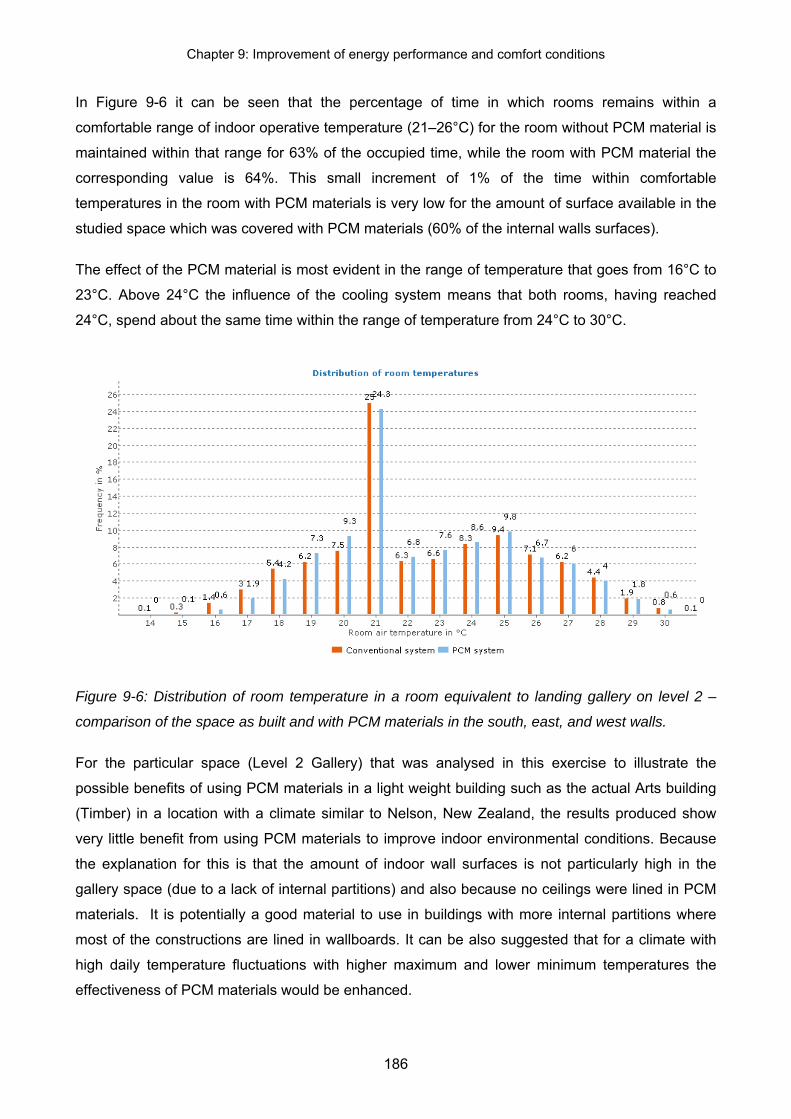
Chapter 9: Improvement of energy performance and comfort conditions
186
In Figure 9-6 it can be seen that the percentage of time in which rooms remains within a
comfortable range of indoor operative temperature (21–26°C) for the room without PCM material is
maintained within that range for 63% of the occupied time, while the room with PCM material the
corresponding value is 64%. This small increment of 1% of the time within comfortable
temperatures in the room with PCM materials is very low for the amount of surface available in the
studied space which was covered with PCM materials (60% of the internal walls surfaces).
The effect of the PCM material is most evident in the range of temperature that goes from 16°C to
23°C. Above 24°C the influence of the cooling system means that both rooms, having reached
24°C, spend about the same time within the range of temperature from 24°C to 30°C.
Figure 9-6: Distribution of room temperature in a room equivalent to landing gallery on level 2 –
comparison of the space as built and with PCM materials in the south, east, and west walls.
For the particular space (Level 2 Gallery) that was analysed in this exercise to illustrate the
possible benefits of using PCM materials in a light weight building such as the actual Arts building
(Timber) in a location with a climate similar to Nelson, New Zealand, the results produced show
very little benefit from using PCM materials to improve indoor environmental conditions. Because
the explanation for this is that the amount of indoor wall surfaces is not particularly high in the
gallery space (due to a lack of internal partitions) and also because no ceilings were lined in PCM
materials. It is potentially a good material to use in buildings with more internal partitions where
most of the constructions are lined in wallboards. It can be also suggested that for a climate with
high daily temperature fluctuations with higher maximum and lower minimum temperatures the
effectiveness of PCM materials would be enhanced.

Chapter 9: Improvement of energy performance and comfort conditions
187
It is unfortunate that the constraints of the VE software used in all of the other modelling analyses
meant that it was unsuited to the task of truly quantifying the effectiveness of PCM materials as a
potential means of increasing the effective thermal mass of the Arts building in a way that would
have negligible structural implications.

Chapter 10: Research conclusions
188
10 Research conclusions:
This chapter summarizes the conclusions and recommendations for further research.
This research has studied the influence of the thermal mass of structural and finishing construction
materials on the space conditioning energy consumption and indoor comfort conditions of medium
sized multi-storey buildings.
A modelling comparison has been undertaken between three very similar medium sized
educational buildings, each designed using structural systems made primarily of timber, concrete
or steel. The concrete and steel buildings have been designed (but not built) to replicate an actual
three-storey 1980 m2 gross floor area educational building, with a timber structure and timber
concrete composite floors. Three additional buildings called the Timber-Low, Concrete-Low and
Steel-Low buildings were designed – also hypothetical - where insulation values of external walls
and roof as well as the glazing and window framing, were significantly increased to a level of best
practice, to reduce the impact of heat losses on the comparison. Each building was modelled with
two different thermal envelopes (code compliant and New Zealand best practice), and different
heating regimes for educational and commercial use, using HVAC system with heating only
(educational scheme) and HVAC system with heating and cooling (commercial scheme).
The analysis of each of these case study buildings includes the modelling of operational energy
use with an emphasis on HVAC energy consumption, and the assessment of indoor comfort
conditions using Predicted Mean Vote (PMV).
In addition to these specific case study buildings, a related but somewhat simpler Test building
model was developed. This was used as a vehicle for investigating the sensitivity of the building’s
thermal behaviour (again assessed by operational energy use and PMV) to changes in the type of
proprietary concrete flooring system used. One outcome of this particular modelling was that it
confirmed that is possible to include an excessive amount of accessible thermal mass, making the
building “sluggish” to changing conditions and even increasing the operational energy requirement
during the occupied hours for which thermal comfort is required.
10.1 Conclusions
In Section 1.3 of the introductory chapter, the original objectives of this research were presented as
a series of eight questions that were to be answered. These same eight questions are repeated
below (Italics), each followed by the corresponding conclusion which has been drawn from the
findings of this work.

Chapter 10: Research conclusions
189
1. Does a concrete, steel, or timber multi-storey building, as currently built in New Zealand,
contain enough thermal mass to have an effect on the space conditioning energy
consumption?
Regardless of whether the buildings are constructed mainly with concrete, steel or timber as the
principal structural and non-structural materials, thermal mass has a relatively low impact on
operational energy consumption for the particular operating regime of the Arts building of this study
– at least in the temperate climate for which the modelling comparison was carried out.
Because, as shown in several previous studies, the operational energy is by far the largest
component of life-cycle energy use, this first conclusion suggests that the life-cycle energy usage
of a building to be used for educational purposes in a temperate climate is relatively insensitive to
the choice of primary structural material.
2. For a concrete, steel, or timber multi-storey building, as currently built in New Zealand, does
the thermal mass influence the indoor environmental conditions?
While the variations in operational energy usage between buildings having different primary
structural materials (timber, concrete and steel) may have been shown to be small, consideration
of environmental comfort – as evidenced by PMV considerations – has shown that the concrete-
based constructions consistently give the smallest number of hours outside the accepted comfort
range.
Nevertheless, the variation in the total hours of out-of-comfort-range conditions is comparatively
small for the three building types within a given level of envelope insulative performance.
Discomfort in buildings in this research most often resulted from overheating of the indoor
environments rather than because environments were cool or cold. It was found that the time in
which the buildings would produce cold/cool environments was similar in the Timber, Concrete,
and Steel buildings. However, when indoor temperature increases, the influence that different
thermal mass materials have in moderating indoor temperatures became more evident in the
amount of hours of warm-to-hot environments.
3. Are there optimal locations for thermal mass materials, and are those locations dependent on
what those materials are?
The influence of thermal mass on comfort conditions varies significantly depending on building
orientation and exposure to solar radiation. While comfort conditions of spaces exposed to the
north were better in the Concrete building than in the Timber building, for example, comfort
conditions in both buildings were very similar in spaces exposed to the south.

Chapter 10: Research conclusions
190
When incident solar radiation is the dominant heat exchange mechanism between thermal mass
and the surrounding environment, concrete thermal mass shows a slow response to temperature
change (slower than air temperature), while timber thermal mass has a very dynamic response to
solar radiation as its surface temperature can increase significantly above air temperature, leading
to the occupants’ perception of more rapidly changing indoor environmental conditions because
mean radiant temperature is a component of perceived thermal comfort.
As a consequence, more comfortable conditions will be achieved in timber buildings if the
incidence of direct solar radiation on to timber surfaces is avoided. In other words, potential
overheating in timber buildings can be controlled by limiting direct solar radiation on internal timber
surfaces.
For a building constructed of mixed (concrete and timber) materials, better indoor environmental
conditions will occur if direct solar radiation impinges on internal concrete surfaces rather than on
internal wood surfaces.
These constraints do not preclude the use of timber as an interior finishing material; for example,
there will be minimal detrimental consequences (and some positive thermal mass benefits) if
exposed timber is used on ceilings generally, and on all interior surfaces in spaces on the south
side of buildings.
These conclusions, which have been deduced from the extensive quantitative modelling
undertaken in this research, are consistent with the common understanding that the most effective
interior locations for surfaces having high thermal mass potential (such as concrete) is where they
will be exposed directly to solar radiation (so-called primary thermal mass).
4. In which way does the improvement of the thermal envelope from code-compliant to best-
practice influence indoor environmental conditions and space energy consumption of
buildings?
Without intervention by the controls of an HVAC system, a consequence of lowering the heat
losses through the thermal envelope by adding insulation is that diurnal temperature swing is
reduced and average indoor temperatures are increased, particularly during summer. The
maximum air and surface temperatures increase during the day, and the minimum temperature
increases during the night.
The immediate consequence of an improved level of insulation from code-compliant to best-
practice is a 10% reduction in heating energy requirements. Although increasing insulation values
in the thermal envelope gives lower heating energy consumption - which is to be expected - this

Chapter 10: Research conclusions
191
also leads to a danger of overheating in summer conditions if insufficient thermal mass is
accessible, and/or inadequate ventilation is provided. In that case mechanical cooling is required
which further increases the energy demand on the building.
5. Are HVAC systems (which are almost always controlled by sensing dry-bulb indoor
temperature), sensitive in any way to the thermal mass available in the three building
structural types?
Despite the presence of thermal mass, indoor environmental conditions are dominantly driven by
HVAC systems, if installed, and thermal mass has a relatively low influence in these conditions.
Forced convection produced by mechanical ventilation tempers the effectiveness of different
thermal mass materials and this is most evident in spaces where convection is the main
mechanism for heat transfer between the air and the thermal mass.
6. Does night-time ventilation improve indoor environmental conditions and subsequently the
response of HVAC systems to the availability of thermal mass in the three building structural
types?
Night-time ventilation is another way of improving the effectiveness of thermal mass as a means of
acting as an energy store and hence buffering heat, and does so in a similar way for all materials.
7. Will good management of direct solar radiation have an impact on the building’s indoor
conditions when concrete or timber are used as thermal mass materials?
External fixed louvres have been shown to increase comfort conditions significantly by reducing the
number of hours in a warm-to-hot environment. By reducing direct solar radiation, convection
became a more relevant heat exchange mechanism. This shift made different thermal mass
materials perform in a similar way.
Paradoxically louvres will produce an increase HVAC energy consumption, particularly in heating
energy, because of the reduction in direct solar gains into the building. In other words, external
louvres can be an effective means of managing direct solar radiation but excessive use of them will
require additional heating energy in winter. (An often-used approach which maintains the shading
benefits of louvres during summer months when the potential for overheating is greatest, but
allows the admission of solar radiation, if desired, during the heating season, is to use louvres fitted
with either manual or BMS-controlled motorized tilting capability. This approach was not modelled
in this research.)

Chapter 10: Research conclusions
192
8. Will phase change material increase the effective thermal mass in a timber-framed building?
Phase change materials (PCM) applied to the timber building as a way of increasing effective
thermal mass in a zone exposed to solar radiation, show little benefits to overall indoor comfort
conditions. Since the space where PCM was modelled was the gallery space, which is an open
space without many internal partitions, not enough surfaces were available to install PCM
materials. PCM would work better in buildings with large areas of available surfaces (walls,
partitions and ceilings) which could be lined with wallboards with embedded PCM.
10.2 Future research
In Section 5.1 one of the reasons for the lack of meaningful results for heating energy consumption
in the Arts building was because there was uncertainty in the operation of the flow meter (and/or
temperature sensors) for the monitoring of heating energy consumption. A calibration of the flow
meters needs to be undertaken; the best way to do this would be to compare flows actually
recorded against a flow alternatively captured with an ultrasonic flow meter. Based on the
outcomes from the calibration of the flow meters, their level of accuracy could be obtained and,
from that, a decision reached on the reliability of the data that has been recorded. In any case, at
least one year’s data has to be analysed to produce any meaningful outcome from monitoring. This
data could then be used for a more reliable calibration of the actual VE model used in this research
and, based on that, new modelling exercises could be performed. Also a real time comparison of
the heating energy consumption between the metered data of the T-Block and the Arts building
could be obtained. That comparison would also act as a benchmark between a concrete and a
timber building. Indoor temperature analysis could also be included in that comparison.
Possible reasons why the models of the Arts building achieve weekly average temperatures which
were about 2°C higher than the monitored temperature during the heating season should be
investigated. Possibly related to this apparent deficiency in the modelling is the fact that for T-block
at least, the diurnal temperature swings predicted by the model were consistently smaller than the
equivalent monitored temperature swings; this too should be investigated.
The versatility and capabilities of building modelling software packages are constantly progressing.
Software that may have become available very recently should be assessed with a view to
possible changing from the one used in this research (which included very extensive HVAC
modelling capability that was particularly useful for some aspects of the current research), to a
modelling software which is able to represent the detail of the building materials, their location and
their behaviour more conveniently.

Chapter 10: Research conclusions
193
Modelling of the buildings was carried out with the finishes and surface materials as installed in the
actual Arts building (e.g. vinyl and carpet). It would be informative to explore the consequences of
changing some or all of these finishing materials (e.g. no floor finishes). In this way it may be
possible to identify more clearly the differences in the energy performance and indoor
environmental conditions of the buildings.
While the simplified, concrete-structured Test building was a useful tool for exploring and
quantifying the energy usage and thermal comfort consequences of adding significantly more
thermal mass to a suspended flooring system, and artificially enhancing the thermal accessibility of
that floor to the air space below, there is other floor-related research that would be worthwhile. This
suggestion is made because the timber buildings modelled in this study had timber-concrete
composite floors, with concrete topping on a timber lower surface. However, more recent multi-
storey timber buildings in New Zealand and overseas have a number of different floor systems.
Some buildings have all-wood floors such as cross-laminated timber flat panels or timber Tee-
beams or timber box beams, with no concrete available as thermal mass at the floor level. Some of
these floors have a suspended ceiling, and others expose the wood to view. Another very different
system (used in the Massey University building in Wellington) has a precast timber-concrete
composite floor system where the 100mm thick concrete slab is visible (and available as thermal
mass) on both the top and bottom surfaces, supported on composite timber floor joists, and timber
beams and columns. The thermal performance of all of these alternative floor systems needs to be
investigated.
Because of its north-facing, three-level gallery space, and the relatively high proportion of glazing
on its south façade, the Arts building, which was the focus of this case study, can be regarded as
being atypical in comparison with the majority of commercial buildings. It would therefore be
informative to conduct a similar modelling comparison on a building which is more representative
of a typical commercial building. It would be desirable to model a more generic building where
simple architectural changes can be made with comparative ease. This would allow, for example, a
sensitivity analysis of the influence of window size on indoor environmental conditions to be
performed.

References
194
References
Alcorn, A. (2010). Materials matter more: Taking the heat out of carbon emissions for New Zealand houses.
Paper presented at the SB10 - New Zealand Sustainable Building Conference.
Aquatherm (2011). Econorad Series Specifications.
ASHRAE (2001, 2009). ANSI/ASHRAE Standard 140 - Standard Method of Test for the Evaluation of
Building Energy Analysis Computer Programs
ASHRAE (2004). Thermal Environmental Conditions for Human Occupancy (ASHRAE Standard 55-2004),
ASHRAE Standard 55-2004. 1791 Tullie Circle NE, Atlanta, GA 30329: ASHRAE.
ASHRAE (2009, 2009). 2009 ASHRAE handbook fundamentals
Aurecon New Zealand Ltd (2009). Mechanical Services Specification NMIT Arts & Media Block.
Balaras, C. A. (1996). The role of thermal mass on the cooling load of buildings. An overview of
computational methods. ENERGY AND BUILDINGS, 24(1), 1-10.
Barnard, N. (1995). Dynamic energy storage in the building fabric (No. TR 9/94). Berkshire: Building Services
Research and Information Association BSRIA.
Barnard, N. (2002). Thermal Mass and Night Ventilation - Utilising "Hidden" Thermal Mass.
INTERNATIONAL JOURNAL OF VENTILATION, 1(2), 81-90.
Barnard, N., Concannon, P., & Jaunzens, D. (2001). Modelling the performance of thermal mass. BRE
Information Paper 6/01
BASF (2011). Micronal ® PCM. In BASF (Ed.), http://www.micronal.de/portal/streamer?fid=443847.
Bellamy, L., & Mackenzie, D. (2001). Thermal performance of buildings with heavy walls (No. 108 (2001)).
Poirirua, New Zealand: Building Research Organisation of New Zealand BRANZ.
Bellamy, L., & Mackenzie, D. (2003). Energy Efficiency of Buildings With Heavy Walls (No. 116 (2003)).
Poirirua, New Zealand: Building Research Organisation of New Zealand.
Bellamy, L., & Mackenzie, D. (2007). Simulation analysis of the energy performance and humidity of solid
wood and light timber frame houses. Pine Manufacturers Association Solid Wood Building
Initiative.
References
195
Box, G. E. P., & Draper, N. R. (1987). Empirical model-building and response surfaces. New York.
Braham, D., Barnard, N., & Jaunzens, D. (2001a). Thermal mass in office buildings: An introduction. Building
Research Establishment digest. Digest 454 Part 1(454), ALL.
Braham, D., Barnard, N., & Jaunzens, D. (2001b). Thermal mass in office buildings: design criteria. Building
Research Establishment digest. Digest 454 Part 2(454), ALL.
Buchanan, A., Palermo, A., Carradine, D., & Pampanin, S. (2011). Post-Tensioned Timber Frame Buildings.
Journal of Structural Engineering, UK, Vol 89(No. 17).
Burgan, B. A., & Sansom, M. R. (2006). Sustainable steel construction. Journal of constructional steel
research, 62(11), 1178-1183.
CIBSE (1986). CIBSE GUIDE A: Design Data. Section A3: Thermal Prperties of Buildings Structures.
London: CIBSE
CIBSE (1998). Building energy and environmental modelling. CIBSE Application Manual AM11:1998.
London: Chartered Institution of Building Services Engineers.
CIBSE (2006). Environmental design : CIBSE guide A. London: CIBSE.
Cole, R. J., & Kernan, P. C. (1996). Life-cycle energy use in office buildings. Building and Environment,
31(4), 307-317.
Corus New Zealand Ltd (2002). ComFlor 210 Composite Floor Decking Retrieved 15 March, 2009, from
http://www.corusnz.com/ComFlorDownloads/Brochures/ComFlor210Brochure%20.pdf
Duffie, J. A., & Beckman, W. A. (2006). Solar engineering of thermal processes (3rd ed.). New York:
Hoboken, N.J.
Eagan, A. (2011). Air tightness of Australian offices buildings: Reality versus typical assumptions used in
energy perfromance simulatrions. Paper presented at the Building Simulation 2011 - 12th
International Conference of the International Building Performance Simulation Association.
Egan, A., M. (2009). Three case studies using building simulation to predict energy perfromance of Australia
office buildings. Paper presented at the Building Simulation 2009 - 11th International
Conference of the International Building Performance Simulation Association.

References
196
EnergyPlus (2010). Auxiliar EnergyPlus Programs - in:
http://apps1.eere.energy.gov/buildings/energyplus/pdfs/auxiliaryprograms.pdf: US Department
of energy.
Gaimster, R., & Munn, C. (2007). The Role of Concrete in Sustainable Development
Gough, M., & Rees, C. (2004). Tests performed on ApacheSim in accordance with ANSI/ASHRAE Standard
140-2001.
Hacker, J. N., De Saulles, T. P., Minson, A. J., & Holmes, M. J. (2008). Embodied and operational carbon
dioxide emissions from housing: A case study on the effects of thermal mass and climate
change. ENERGY AND BUILDINGS, 40(3), 375-384.
Halliday, J. (2010). Underfloor Heating Zone Capacities. In N. Perez (Ed.). Chrischurch: Aurecon New
Zealand Limited.
Hand, J., Kim, J., & Woo, K. (2011). Gaining confidence in the models of experiments in existing buildings.
Paper presented at the Building Simulation 2011 - 12th International Conference of the
International Building Performance Simulation Association.
IES Ltd (2009). Virtual Environment Construccion Database user guide - available at
http://www.iesve.com/downloads/help/Thermal/ConstructionsDatabase.pdf
IES Ltd (2010a). Apache HVAC user guide - available at
http://www.iesve.com/downloads/help/Thermal/ApacheHVAC.pdf.
IES Ltd (2010b). Virtual Environment. Glasgow: Integrated Environmental Solutions (IES) Ltd.
IES Ltd (2011). ApacheSim Calculation Methods - available at
http://www.iesve.com/downloads/help/ve64/Thermal/Reference/ApacheSimCalculationMethods.
IFIAS (1974). Energy analysis workshop on methodology and convention, Workshop Report No. 6
Stockholm: International Federation of Institutes for Advanced Study.
Ip, K., Dyball, D., & Miller, A. (2008). Thermal behaviour of wall-lining containing Phase Change Materials.
Paper presented at the 2008 World Sustainable Building Conference.
Irving Smith Jack Architects Ltd (2008). NMIT Arts and Media Buildings Timber Demostration Project Design
Competition. Ref DC464.

References
197
John, S., Nebel, B., Perez, N., & Buchanan, A. (2008). Environmental impacts of Multi-storey buildings using
different construction materials Christchurch: University of Canterbury, Scion, Victoria
University,.
Kembla (2011). Kembla PEX Water Solutions, from
http://www.kembla.co.nz/PRODUCTS/KEMBLA+PEX+WATER+SOLUTIONS.html
Leslie, S. F. (1976). Annual heating energy demand of heavy domestic buildings. Auckland, New Zealand:
Report / New Zealand Energy Research and Development Committee ; no. 16.
Liley, B. (2011). Personal comunication with Ben Linley about Nelson hourly global, direct & diffuse radiation.
In M. Kean (Ed.). Christchurch.
Lowenstein, O. (2009). Towering impact - Timber construccion reaches for the sky. Green Building
Magazine, 19, 48 - 52.
Meteotest (2011). Meteonorm software. Bern: http://meteonorm.com/.
Mithraratne, N., & Vale, B. (2004). Life cycle analysis model for New Zealand houses Building and
Environment, 39(4), 483-492.
Moore, T. C. (2008). Simulation of radiant cooling performance with evaporative cooling sources. University
of California, Berkeley, Berkeley.
Nebel, B., Alcorn, A., & Wittstaock, B. (2009). Life Cycle Assessment: Adopting and adapting overseas LCA
data and methodologies for building mateials in New Zealand. Wellington.
Neymark, J., & Judkoff, R. (2002, 2002). International Energy Agency Building Energy Simulation Test and
Diagnostic Method for Heating, Ventilating, and Air-Conditioning Equipment Models (HVAC
BESTEST); Volume 1 Cases E100-E200, from http://www.osti.gov/servlets/purl/15000340-
OZL9Os/native/
NIWA (2011). The Climate of New Zealand - Northern South Island, from http://www.niwa.co.nz/education-
and-training/schools/resources/climate/overview/map_n_south
NIWA National Institute of Water & Atmospheric Research (2011). CliFlo National Climate Database, from
http://cliflo.niwa.co.nz/

References
198
NZGBC (2009). CLimate change and the built environment. Available at:
http://www.nzgbc.org.nz/images/stories/downloads/public/Knowledge/reading/ClimateChange_B
uiltEnviro_NZGBC.pdf.
NZS (2006). NZS 4214:2006 Methods of determining the total thermal resistance of parts of buildings.
Wellington [N.Z]: Standards New Zealand.
NZS (2007). NZS 4243.1:2007 Energy efficiency - Large buildings Part 1: Building Thermal Envelope.
Wellington [N.Z.]: Standards New Zealand.
Page, I. (2006). E408 Timber in Government buildings - cost and environmental impact analysis (No.
QC5018). Porirua: BRANZ Limited.
Pan, Y., Huang, Z., & Wu, G. (2007). Calibrated building energy simulation and its application in a high-rise
commercial building in Shanghai. ENERGY AND BUILDINGS, 39(6), 651-657.
Pedrini, A., Westphal, F. S., & Lamberts, R. (2002). A methodology for building energy modelling and
calibration in warm climates. Building and Environment, 37(8-9), 903-912.
Pereira, C., D., & Ghisi, E. (2011). Calibration of a computer model of a natural ventilated house located in
southern Brazil. Paper presented at the Building Simulation 2011 - 12th International
Conference of the International Building Performance Simulation Association.
Perez, N. (2008). The influence of construction materials on life-cycle energy use and carbon dioxide
emissions of medium size commercial buildings Unpublished Master Thesis Victoria University
of Wellington, Wellington.
Perez, N., Baird, G., & Buchanan, A. (2008). The influence of construction materials on life-cycle energy use
and carbon dioxide emissions of medium size commercial buildings Paper presented at the
2008 World Sustainable Building Conference.
Raftery, P., Keane, M., & Costa, A. (2009). Calibration of a detailed simulation model to energy monitoring
system data: A methodology and case study. Paper presented at the Building Simulation 2009 -
11th International Conference of the International Building Performance Simulation Association.
Reddy, T. A., Maor, I., & Panjapornpon, C. (2007). Calibrating Detailed Building Energy Simulation Programs
with Measured Data-Part I: General Methodology (RP-1051). HVAC&R Research, 13(2), 221-
241.
Roberts, S. (2008). Effects of climate change on the built environment. Energy Policy, 36(12), 4552-4557.

References
199
Sathre, R. (2007). Life-cycle energy and carbon implications of wood-based products and construction. s.n.],
S.l.
Sathre, R., & Gustavsson, L. (2008). Using wood products to mitigate climate change: External costs and
structural change. Applied Energy, 86(2), 251-257.
Schneider Electric (2011). Schneider Electric New Zealand, from http://www.schneider-
electric.com/site/home/index.cfm/nz/
Sellin, A. (2011). Personal comunication with Antony Selling. October 2011. Christchurch.
Simonson, C. J., Salonvaara, M., & Ojanen, T. (2001). Improving indoor climate and comfort with wooden
structures, VTT Publications (pp. X-200).
Srinivasan, R., S., Lakshmanan, J., & Srivastav, D. (2011). Calibrated simulation of an existing convention
centre: the role of event calendar and energy modeling software. Paper presented at the
Building Simulation 2011 - 12th International Conference of the International Building
Performance Simulation Association.
Standards New Zealand (2006a). NZS 4214:2006 Methods of determining the total thermal resistance of
parts of buildings. Wellington [N.Z]: Standards New Zealand.
Standards New Zealand (2006b). NZS 4303:1990 Ventilation for acceptable indoor air quality. Wellington
[N.Z]: Standards New Zealand.
Standards New Zealand (2007). NZS 4243.2:2007 Energy efficiency - Large buildings Part 2: Lighting.
Wellington [N.Z.]: Standards New Zealand.
Swegon (2010). Parasol - Integrated Comfort Modules. Downlodable from:
http://www.swegon.com/en/Products/Waterborne-Climate-Systems/Comfort-Modules/.
Stokholm: Swegon,.
Thompson, G. (2006). Thermal mass for housing. Concrete, 40(10), 86-86-87.
U.S. Department of Energy (2010). Building Energy Software Tools Directory, from
http://apps1.eere.energy.gov/buildings/tools_directory/
US Department of Energy (2010). EnergyPlus Energy Simulation Software -
in:http://apps1.eere.energy.gov/buildings/energyplus/.

References
200
Valentin Energiesoftware (2011). PCM Express. Berlin, Germany: Dr. Valentin EnergieSoftware GmbH.
WGBC (2011). Tackling global climate change meeting local priorities. Available in:http:
//www.worldgbc.org/site2/resources/.
Yang, L., & Li, Y. (2008). Cooling load reduction by using thermal mass and night ventilation. Energy and
Buildings, 40(11), 2052-2058.

Appendices
201
Appendices:
A. Modelling of the test building and its comparison with the Arts building:
Figure A-1: Comparison of the plan section on Level 1 of the test building (a) and the Arts building
(b).
a. b.

Appendices
202
(a) (b)
Figure A-2: Schematic network of the HVAC system - educational (a) and commercial (c) - in
Virtual Environment’s Apache HVAC tool, and schematic of an induced air (Parasol ®) unit in (b).

Appendices
203
B. Representation of Solar Insolation in VE Apache
As was mentioned in Section 3.9.1, within VE Apache the required solar tracking algorithms are
contained within the SunCast module. Normally the inner workings of these calculations are
invisible to the user, but it is possible to access generated tables which illustrate how the insolation
incident upon a surface of interest (either external or internal) is resolved and quantified as an input
to the thermal modelling of that surface. This may be helpful in interpreting in particular the
consequences of solar insolation which is incident upon the surface of a thermal mass element.
(a) (b)
Figure B-1: an interior view of Level 2 of the simplified model, without internal stand-alone walls
(a), and with internal stand-alone walls (b). (1) Identifies an external wall, and (2) identifies one of
the internal stand-alone-walls.
Figure B-1 shows the location of two representative walls in the Test building model for which
measurements of area of insolation as a percentage of the surface area of walls (external and
internal) are further represented in a flexigrid format in Table B-1, Table B--2, and Table B-3.
These tables illustrate the way in which SunCast tracks solar intensity values across external and
internal walls as if they are experiencing each hour the average solar intensity value uniformly over
the entire component.
Table B-1: Exterior wall (1), external insolation type.
Month 1:00 2:00 3:00 4:00 5:00 6:00 7:00 8:00 9:00 10:00 11:00 12:00 13:00 14:00 15:00 16:00 17:00 18:00 19:00 20:00 21:00 22:00 23:00 0:00Jan 0 0 0 100 100 100 100 100 100 100 100 0 0 0Feb 0 0 100 100 100 100 100 100 100 100 100 100 0 0Mar 100 100 100 100 100 100 100 100 100 100 100 100Apr 100 100 100 100 100 100 100 100 100 100May 100 100 100 100 100 100 100 100 100 100Jun 100 100 100 100 100 100 100 100 100Jul 100 100 100 100 100 100 100 100 100 100Aug 100 100 100 100 100 100 100 100 100 100Sep 100 100 100 100 100 100 100 100 100 100 100 100Oct 0 100 100 100 100 100 100 100 100 100 100 100 0Nov 0 0 100 100 100 100 100 100 100 100 100 0 0 0Dec 0 0 0 0 100 100 100 100 100 100 100 100 0 0 0
1.
2.

Appendices
204
Table B-1 shows the calculation of the shading results for the design day (15th of each month)
during every month, displayed in flexigrid format and showing the area of insolation as a
percentage of the surface area. In the case of external walls, both external and internal insolation
data can be extracted, as can be seen in Table B–2 and Table B-3 respectively.
Table B--2: Exterior wall (1), internal insolation type.
Month 1:00 2:00 3:00 4:00 5:00 6:00 7:00 8:00 9:00 10:00 11:00 12:00 13:00 14:00 15:00 16:00 17:00 18:00 19:00 20:00 21:00 22:00 23:00 0:00Jan 0 0 0 0 0 0 0 0 0 0 0 0 35 23.2Feb 0 0 0 0 0 0 0 0 0 0 0 0 0 36.6Mar 0 0 0 0 0 0 0 0 0 0 0 0Apr 0 0 0 0 0 0 0 0 0 0May 0 0 0 0 0 0 0 0 0 0Jun 0 0 0 0 0 0 0 0 0Jul 0 0 0 0 0 0 0 0 0 0Aug 0 0 0 0 0 0 0 0 0 0Sep 0 0 0 0 0 0 0 0 0 0 0 0Oct 0 0 0 0 0 0 0 0 0 0 0 0 17.9Nov 0 0 0 0 0 0 0 0 0 0 0 0 33.3 19Dec 0 0 0 0 0 0 0 0 0 0 0 0 16.5 27.9 19.3
Table B-3: Internal wall (2), internal insolation type
Month 1:00 2:00 3:00 4:00 5:00 6:00 7:00 8:00 9:00 10:00 11:00 12:00 13:00 14:00 15:00 16:00 17:00 18:00 19:00 20:00 21:00 22:00 23:00 0:00Jan 0 0 0 3.4 1.9 0 0 0 0 0 0 0 0 0Feb 0 2 3.7 2.6 3 6.1 8.5 0 0 0 0 0 0 0Mar 6.3 18.4 28.6 36.9 37.5 34.8 0 0 0 0 0 0Apr 51.1 50.8 48.6 47.5 38.9 0 0 0 0 0May 58.3 65.2 59.7 57 41.8 0 0 0 0 0Jun 51.6 70 64.6 61.4 51.8 0 0 0 0Jul 53.1 69.3 63.2 59.9 53.3 0 0 0 0 0Aug 59 59.4 54.5 51.9 44.7 0 0 0 0 0Sep 24.6 38.8 38.9 43.1 42.7 28.3 0 0 0 0 0 0Oct 17.9 1.9 3 7.3 13.5 17.1 0 0 0 0 0 0 0Nov 0 0 3 2.6 0.6 0.1 0 0 0 0 0 0 0 0Dec 0 0 0 0 3.3 1.8 0 0 0 0 0 0 0 0 0
Table B-3 similarly shows the calculation of the shading results for the design day during every
month, for the case of an internal wall for which only internal insolation data is available.

Appendices
205
C. Constructions
Table C-1: Timber, concrete and steel buildings; R – C values of materials
TIMBER CONCRETE STEEL∑R ∑C ∑R ∑C ∑R ∑C
Windows0.25 15.0 0.25 15.0 0.25 15.0
0.32 11.3 0.32 11.3 0.32 11.3
External wall2.81 20.7 2.81 20.7 2.81 20.7
2.74 172.3 1.41 463.2
Internal wall2.70 26.0 2.70 26.0 2.70 26.0
1.45 169.4 0.13 460.0
Suspended ceilings2.70 30.7 2.70 30.7 2.70 30.7
0.31 19.6 0.31 19.6 0.31 19.6
Structural suspended floor1.12 248.3 0.73 245.4 0.42 284.4
0.78 249.0 0.40 246.1 0.08 285.1
Concrete suspended floor0.13 428.4 0.13 428.4 0.13 428.4
External glazing
External glazing
External glazing
Internal glazing
Internal glazing
Internal glazing
External light wall
External light wall
External light wall
External shear wall
LVL
External shear wall Concrete
Internal partitions
light
Internal partitions
light
Internal partitions
lightInternal
shear wall LVL
Internal shear wall Concrete
Gib board Gib board Gib board
Comflor carpet
Acoustic tile
Acoustic tile
Acoustic tile
Potius vinyl
Interspa vinyl
Comflor vinyl
Potius carpet
Interspan carpet
Suspended concrete
floor
Suspended concrete
floor
Suspended concrete
floor

Appendices
206
Table C--2: Continuation of Table A-1 – ‘Timber, concrete and steel buildings; R – C values of
materials’.
TIMBER CONCRETE STEEL∑R ∑C ∑R ∑C ∑R ∑C
External overhang floor5.07 196.7 5.07 196.7 5.07 196.7
5.15 461.2 5.15 461.2 5.15 461.2
Roof5.12 55.9 5.12 55.9 5.12 55.9
4.01 28.5 4.01 28.5
Heated slab0.09 106.5 0.09 106.5 0.09 106.5
0.09 105.6 0.09 105.6 0.09 105.6
Slab on gound3.44 1545.9 3.44 1545.9 3.44 1545.9
3.41 1440.1 3.41 1440.1 3.41 1440.1
Floor cantilever
ligt
Floor cantilever
ligt
Floor cantilever
ligtFloor
cantilever heavy
Floor cantilever
heavy
Floor cantilever
heavy
Heated slab- vinyl
Heated slab- vinyl
Heated slab- vinyl
Roof steel
Roof steel
Roof timber
Roof timber
Roof timber
Slab on ground
Slab on ground
Slab on ground
Heated slab- clear
Heated slab- clear
Heated slab- clear
Slab on ground- heated
Slab on ground- heated
Slab on ground- heated
The constructions highlighted in grey are those that are unique for that particular building, whereas
non-highlighted constructions are common to the four buildings. For instance, in ‘Windows’
constructions the same external glazing is used in the Timber, Concrete, and Steel buildings but an
external glazing with a higher R-value is used in the Timber-Low building.

Appendices
207
Table C-3: Timber-low, concrete-low, steel-low buildings; R – C values of materials
TIMBER-LOW CONCRETE-LOW STEEL_LOW∑R ∑C ∑R ∑C ∑R ∑C
Windows0.50 15.0 0.50 15.0 0.50 15.0
0.32 11.3 0.32 11.3 0.32 11.3
External wall4.55 21.2 4.55 21.2 4.55 21.2
4.20 173.2 2.87 464.2
Internal wall2.70 26.0 2.70 26.0 2.70 26.0
1.45 169.4 0.13 460.0
Suspended ceilings2.70 30.7 2.70 30.7 2.70 30.7
0.31 19.6 0.31 19.6 0.31 19.6
Structural suspended floor1.12 248.3 0.73 245.4 0.42 284.4
0.78 249.0 0.40 246.1 0.08 285.1
Concrete suspended floor0.13 428.4 0.13 428.4 0.13 428.4
PVC frame;
Argon filled
External glazing
External glazing
Internal glazing
Internal glazing
Internal glazing
External light wall
-low
External light wall
-low
External light wall
-lowExternal
shear wall LVL- low
External shear wall
concrete
Internal partitions
light
Internal partitions
light
Internal partitions
lightInternal
shear wall LVL
Internal shear wall
concrete
Gib board
Gib board
Gib board
Potius carpet
Interspan carpet
Comflor carpet
Acoustic tile
Acoustic tile
Acoustic tile
Potius vinyl
Interspa vinyl
Comflor vinyl
Suspended concrete
floor
Suspended concrete
floor
Suspended concrete
floor

Appendices
208
Table C-4: Continuation of Table A-3 – ‘Timber-low, concrete-low, steel-low buildings; R – C values
of materials’.
TIMBER-LOW CONCRETE-LOW STEEL_LOW∑R ∑C ∑R ∑C ∑R ∑C
External overhang floor5.07 196.7 5.07 196.7 5.07 196.7
5.15 461.2 5.15 461.2 5.15 461.2
Roof9.41 48.0 9.41 48.0 9.41 48.0
Heated slabHeated
slab- 0.09106.5 Heated
slab 0.09106.5 Heated
slab 0.09106.5
Heated 0.09 105.6 Heated 0.09 105.6 Heated 0.09 105.6
Slab on goundSlab on ground 3.44
1,546Slab on ground 3.44
1,546Slab on ground 3.44
1,546
3.41 1,440 3.44 1,546 3.44 1,546
Floor cantilever
ligt
Floor cantilever
ligt
Floor cantilever
ligt
Roof timber
-low
Roof timber
Roof timber
Floor cantilever
heavy
Floor cantilever
heavy
Floor cantilever
heavy
Slab on ground heated
Slab on ground heated
Slab on ground heated

Appendices
209
D. Thermal templates
Table D-1: Level 2 thermal zones area and volume.
Level 1 - Conditioned thermal zones
Area (m2)
Volume (m3)
Level 1 - Unconditioned thermal zones
Area (m2)
Volume (m3)
Computer room Storage & circulation_CoreComputer 84.4 314.9 Storage Seminar 8.7 22.5Office_Core Link Corridors 34.2 88.3Interview 8.9 33.3 Link Seminar-Gallery 10.3 26.6DB-Comms 9.1 23.4 Storage & circulation_PerimeterReception-Mail 19.3 51.7 Fire Stair 18.3 76.3Office_Perimeter Unoccupied & Voids & MassStaff-Program leader 22.6 84.5 Ceiling_Link Corridor 10.3 14.8Head of Sch-Program leader 19.7 73.4 Ceiling Concrete_Computer 27.7 9.6Classroom_Perimeter Ceiling_Computer 56.9 23.7Textile 79.7 326.9 Services 9.8 40.7Seminar 61.0 203.5 Lift 10.5 43.8Gallery Ceiling_DB-Comms 9.1 13.3Gallery 1st Floor 211.4 862.9 Ceiling_Link 7.3 10.8
∑ 516 1,975 Ceiling_Link Corridors 34.2 50.2Ceiling_Reception-Mail 19.3 28.3Ceiling Concrete_Textile 0.9 1.0Ceiling Concrete_RM 114-116 15.7 5.4Ceiling_RM 113-114-115-118 37.0 15.4Ceiling-Seminar 45.3 18.9Ceiling Concrete_Seminar 15.8 5.5
∑ 371 495
Table D-2: Level 2 thermal zones area and volume.
Level 2 - Conditioned thermal zones
Area (m2)
Volume (m3)
Level 2 - Unconditioned thermal zones
Area (m2)
Volume (m3)
Gallery Storage & circulation_CoreGallery Void 3.1 326.2 Link 5.9 15.3Landing-Gallery 104.4 401.9 Link 5.7 14.7Office_Perimeter Storage & circulation_PerimeterStaff 46.8 180.3 Storage-Duct 6.0 23.2Classroom_Perimeter Fire Stairs 18.4 70.9Studio 328.3 1,264.2 Unoccupied & Voids & MassToilets Lift 10.6 40.7DB-Toilet 9.1 23.5 Ceiling_Link 7.7 8.8Toilets-Storage 19.4 50.1 Ceiling_Link 7.4 8.5
∑ 511 2,246 Ceiling_Toilet 9.1 10.5Ceiling_Toilets-Storage 19.4 22.3Ceiling Concrete_Studio 9.6 5.2
∑ 100 220

Appendices
210
Table D-3: Level 3 thermal zones area and volume.
Level 3 - Conditioned thermal zones
Area (m2)
Volume (m3)
Level 3 - Unconditioned thermal zones
Area (m2)
Volume (m3)
Office_Perimeter Storage & circulation_CoreStaff meet 34.7 100.1 Fire Stairs 18.4 67.5Staff 49.3 142.1 Storage staff 3.9 14.4Classroom_Perimeter Store 9.0 23.3Drawing Central 82.5 316.2 Storage & circulation_PerimeterDrawings West 82.5 316.2 Corridor Studios 32.0 82.6Studio seminar 81.7 313.6 Unoccupied & Voids & MassDrawings East 82.0 348.2 Lift 10.6 38.8Gallery Ceiling-roof_DB-Toilet 9.1 8.8Ceiling-Roof_Staff 34.0 57.3 Ceiling-roof_Toilet-Storage 19.4 18.8Ceiling-Roof_Gallery 95.7 222.9 Ceiling-roof_Link 7.4 7.1Gallery 67.4 190.5 Ceiling-roof_Link 7.7 7.4L3_Void 4.4 281.2 Ceiling-roof_Staff-Corridor 15.7 10.4Toilets ∑ 133 279DB-Toilets 9.1 23.5Toilet-Storage 19.4 50.1
∑ 643 2,362

Appendices
211
E. Mechanical Ventilation and heating data
Table E-1: Educational HVAC system’s mechanical ventilation and radiant heating data.
Direct Indirect R - 1 (4.6 kW)
R - 2 (3.8 kW)
R - 3 (2.7 kW)
Level 1 Computer roomComputer 250Office_CoreInterview 30 0.6Reception-Mail 30 2.2Office_PerimeterStaff-Program leader 1.3Head of Sch-Prg led. 1.2Classroom_PerimeterTextile 125 5.0Seminar 125 3.4GalleryGallery 1st Floor 560 560 12.3
∑ 560 560 560 0.0 0.0 0.0 26.0Level 2 GalleryGallery Void 750Landing-Gallery 750 4.6 3.8Office_PerimeterStaff 125 4.6Classroom_PerimeterStudio 625 23.0 8.1
∑ 750 750 750 9.2 26.9 8.1 0.0Level 3 Office_PerimeterStaff meet 125 3.8Staff 125 4.6Classroom_PerimeterDrawing Central 125 3.8 2.7Drawings West 125 3.8 2.7Studio seminar 125 4.6 3.8Drawings East 125 4.6 3.8GalleryGallery 750 4.6Ceiling-Roof_StaffCeiling-Roof_Gallery
L3_Void
∑ 750 750 2060 18.4 19.2 5.4 0.0
2060
Thermal template &
Room name
Mechanical Ventilation HeatingSupply (L/s)
Return (L/s)
Radiators Underfloor heating (kW)

Appendices
212
Table E-2: Commercial HVAC system’s mechanical ventilation and radiant heating data.
Direct Indirect Heating (kW)
Cooling (kW)
R - 1 (4.6 kW)
R - 2 (3.84 kW)
Level 1 Computer roomComputer 250Office_CoreInterview 30 2.7 2.1Reception-Mail 30 2.7 2.1Office_PerimeterStaff-Program leader 5.1 6.3Head of Sch-Prg led. 5.1 6.3Classroom_PerimeterTextile 125 2.7 2.1Seminar 125 2.7 2.1GalleryGallery 1st Floor 560 560 12.3
∑ 560 560 560 21.1 20.8 0.0 0.0 12.3Level 2 GalleryGallery Void 750Landing-Gallery 750 4.6 3.8Office_PerimeterStaff 125 2.7 2.1Classroom_PerimeterStudio 6265 13.5 10.3
∑ 6390 750 750 16.2 12.3 4.6 3.8 0.0Level 3 Office_PerimeterStaff meet 125 2.7 2.1Staff 125 2.7 2.1Classroom_PerimeterDrawing Central 125 2.7 2.1Drawings West 125 2.7 2.1Studio seminar 125 2.7 2.1Drawings East 125 2.7 2.1GalleryGallery 750 4.6Ceiling-Roof_StaffCeiling-Roof_GalleryL3_Void
∑ 750 750 2060 16.2 12.3 4.6 0.0 0.0
Parasol Units Radiators Underfloor heating (kW)
Mechanical Ventilation
Return (L/s)
Supply (L/s)
2060
Heating + CoolingThermal template
& Room name
Table E-1 and Table E-2 show the specific flow of mechanically supplied air into each conditioned
space in the actual Arts building; data is organized by levels. Air flow is primarily subdivided in
‘Supply’ and ‘Return’, subsequently only ‘Supply’ is subdivided into ‘Direct supply’ and ‘Indirect
Supply’. The rationale behind the sub-classification of ‘Supply’ is based in Figure 4-9 Section 4.6.1
of the thesis main document, where the mechanical air distribution network by levels is subdivided
in four segments being: A, B, C, and D.

Appendices
213
F. THERM analysis of under-floor heated slab conductivity
To simulate an embedded pipe, a section, of the heated slab in between pipes was cut. The
boundary condition of the water: T=40°C and λ=5000 W/m2K, maintaining all the layers of the floor,
as represented in Figure F-.
Material Conductivity (W/(m*K))
Emissivity
1 Vinyl 0.79 0.92 PEX (Tubing) 0.38 0.93 Cast Concrete 1.6 0.554 EPS 0.025 0.9
Boundary Conditions
Temperature (°C)
Film Coeffcient
2A Inside 20 7.7B PEX
(Inside tubing)40 5000
C Adiabatic 0 0
Figure F-1: A cross-section of the concrete slab with embedded hydronic tubing is described in
THERM as a repeatable segment bounded by the heated surface (top), centre of the tubing
(sides), and midpoint between tubes (either side). Boundaries other than the tube interiors and
heated surface are adiabatic.
Figure F-2: Colorized/shaded and isothermal contours indicate the distribution of temperatures
resulting from the finite-element model of two-dimensional heat transfer between boundary
conditions.

Appendices
214
Vertical lines trough the pipes became lines of symmetry that represent adiabatic boundaries on
the THERM model which is a correct representation of a recurring pattern of hydronic pipes. The
resistance at the top surface value of 0.12 m2K/W and, with a modelled average surface
temperature of 31.8°, the heat flow into the air above (22 °C) was determined to be 90 W/m2.
For steady state, the same upward rate of heat flow must be taking place through the concrete
below the pipes, so for a truly 1-D floor model with a uniform layer of 40° C water at a depth of
50mm below the top surface, an effective thermal conductivity of 0.548 W/mK for the cast concrete
was determined.
Node Temperature [°C]
26 32.940 32.850 31.660 30.769 30.479 30.782 31.680 32.870 32.9
Average 31.8
Figure F-3: Finite-element mesh at section through bisected hydronic tubing – table indicating
nodes number and temperature at node.
Figure F-33 presents a simple way of checking the consistency of the initial TERM model which
was undertaken. A new THERM model was set up consisting of a uniform slab of concrete, 50mm
thick and having the deduced thermal conductivity value (0.55 W/mK). A bottom boundary
condition of water at 40° C with the same extremely high effective conductivity from water to
concrete as the existing model has between water and PEX was imposed. The upper boundary
condition should be exactly the same as in the existing model, i.e. convection to air at 22°C. The
simple slab model results in a uniform upper surface temperature of 31.8° C.
4
C C

Appendices
215
G. Influence of steel purlins on space conditioning energy
Table G-1: Total and end-use energy consumption for the Timber building, the Concrete building
(with steel purlins in the roof), and the Steel building (with steel purlins in the roof).
R C R C R C R C R C R C R C ∑R ∑C0.04 0.0 0.00 2.2 0.14 24.8 4.56 1.2 0.20 17.6 0.07 10.1 0.10 0.0 5.12 55.9
0.04 0.0 0.00 2.2 0.14 16.1 3.81 1.4 0.06 8.7 0.10 0.0 4.01 28.5
Gib Board Inside surface
Roof Steel Purlins
Outside surface
Profiled Steel
Plywood Bridged Insulation
Gib Board Inside surface
Roof Timber Purlins
Outside surface
Profiled Steel
Plywood Bridged Insulation
Timber
C: KJ/m2KR: m2K/W
Table G-2: Total and end-use energy consumption for the Timber building, the Concrete building
(with steel purlins in the roof), and the Steel building (with steel purlins in the roof).
Thermal Electric Thermal Electric Thermal Electric Thermal Electric Thermal ElectricHeating 66.9 1.1 69.4 1.2 70.6 1.2 68.1 1.1 69.3 1.1Chillers 0.0 0.7 0.0 0.6 0.0 0.6 0.0 0.7 0.0 0.7Fans 0.0 5.7 0.0 5.7 0.0 5.7 0.0 5.7 0.0 5.7DHW 0.0 20.1 0.0 20.1 0.0 20.1 0.0 20.1 0.0 20.1Lighting 0.0 21.3 0.0 21.3 0.0 21.3 0.0 21.3 0.0 21.3Equipments 0.0 7.5 0.0 7.5 0.0 7.5 0.0 7.5 0.0 7.5∑ 66.9 56.4 69.4 56.4 70.6 56.4 68.1 56.4 69.3 56.4Total (MWh)
Concrete Builiding Steel BuildingTimber
Timber Purlins Timber Purlins
123.3 125.8 124.5
Steel Purlins Steel Purlins
127.1 125.7

Appendices
216
Timber Purlins Timber Purlins Steel Purlins Timber Purlins Steel PurlinsTimber Concrete Builiding Steel Building
Heating (Thermal) 66.9 69.4 70.6 68.1 69.3Heating (Electric) 1.1 1.2 1.2 1.1 1.1Chillers (Electric) 0.7 0.6 0.6 0.7 0.7Fans (Electric) 5.7 5.7 5.7 5.7 5.7DHW (Electric) 20.1 20.1 20.1 20.1 20.1Lighting (Electric) 21.3 21.3 21.3 21.3 21.3Equipments (Electric) 7.5 7.5 7.5 7.5 7.5Total (Combined) 123.3 125.8 127.1 124.5 125.7
0
20
40
60
80
100
120
140M
Wh
Figure G-3: Total and end-use energy consumption for the Timber building, the Concrete building
(with steel purlins in the roof), and the Steel building (with steel purlins in the roof).

Appendices
217
H. Variable PMV assessment
Table H-1: Comfort parameters for PMV calculations – Alternative to default values.
Comfort parameters in winter conditionsClothing levels: 1 clo Male / Office / Medium From 1/JAN to 14/MARActivity Levels 69.8 W/m2 Sedentary work, standing From 15/OCT to 31/DEC
Comfort parameters in summer conditionsClothing levels: 0.2 clo Sportwear From 15/MAR to 14/OCTActivity Levels 69.8 W/m2 Sedentary work, standing
Timber Concrete Steel Timber - low
Concrete - low
Steel - low
Timber - low
Concrete - low
Steel - low
Educational Educational Commercial< -0.50 1287 1358 1302 1000 1049 921 1221 1285 1251-0.50 to 0.50 1273 1380 1378 1201 1292 1381 1144 1216 1207> 0.50 571 392 451 929 790 828 766 630 673
0
500
1000
1500
2000
2500
3000
Hou
rs
Variable PMV - Landing gallery
Figure H-1: Variable PMV analysis of Landing-Gallery space on level 2, north facing.

Appendices
218
Timber Concrete Steel Timber - low
Concrete - low
Steel - low
Timber - low
Concrete - low
Steel - low
Educational Educational Commercial< -0.50 1218 1235 1195 1076 1128 1011 1388 1379 1383-0.50 to 0.50 1327 1458 1510 1337 1428 1516 1508 1624 1608> 0.50 586 438 425 718 575 603 234 128 139
0
500
1000
1500
2000
2500
3000
Hou
rsVariable PMV - Staff room
Figure H-2: PMV of Staff room on level 2, north facing.
Timber Concrete Steel Timber - low
Concrete - low
Steel - low
Timber - low
Concrete - low
Steel - low
Educational Educational Commercial< -0.50 1489 1607 1497 1146 1161 1078 1494 1506 1540-0.50 to 0.50 1621 1522 1615 1912 1910 1977 1632 1622 1585> 0.50 21 2 19 73 60 76 5 3 5
0
500
1000
1500
2000
2500
3000
Hou
rs
Variable PMV - Studio 201
Figure H-3: PMV of Studio 201 on level 2, south facing.

Appendices
219
I. PCM analysis
Table I-1: Materials used in the analysis done in PCM-Express software.
Thickness (m)
Conductivity (W/(m*K))
Density Kg/m3
Specific Heat
Capacity KJ/(kg*K)
1 Suspended floor construccion1.1 Arts_Suspended floor slab (Potius)
Cork linoleoum (THAM) 0.003 0.08 700 1.6DIN EN 12524 Reinforced concr. 0.075 2.50 2400 1.0DIN EN 12524 Timber materials Plywood 0.095 0.10 500 1.5
2 Roof construccions2.1 Roof sloping roof (SmartBoard 23)
Micronal PCM SmartBoard 23 0.015 0.20 770.0 Depending on temp.
Glass Wool (THAM) 0.190 0.04 30.0 1.0DIN EN 12524 Timber materials Plywood 0.012 0.10 500 1.5Air Layer (THAM) 0.055 0.05 1.0 1.0Roof tile (THAM) 0.010 0.75 1500.0 0.9
2.2 Roof sloping roof (GIB)DIN EN 12524 Plasterboard panels 900 0.015 0.25 900.0 1.0Glass Wool (THAM) 0.190 0.04 30.0 1.0DIN EN 12524 Timber materials Plywood 0.012 0.10 500 1.5Air Layer (THAM*) 0.055 0.05 1.0 1.0Roof tile (THAM*) 0.010 0.75 1500.0 0.9
3 Internal partitions3.1 Internal wall (GIB)
DIN EN 12524 Plasterboard panels 900 0.015 0.25 900.0 1.0Glass Wool (THAM*) 0.100 0.04 30.0 1.0DIN EN 12524 Plasterboard panels 900 0.015 0.25 900.0 1.0
3.2 Internal wall (SmartBoard 23)
Micronal PCM SmartBoard 23 0.015 0.20 770.0 Depending on temp.
Glass Wool (THAM*) 0.100 0.04 30.0 1.0
Micronal PCM SmartBoard 23 0.015 0.20 770.0 Depending on temp.

Appendices
220
Table I-2: Materials used in the analysis done in PCM-Express software.
Thickness (m)
Conductivity (W/(m*K))
Density Kg/m3
Specific Heat
Capacity KJ/(kg*K)
3 External walls3.1 External wall (GIB)
DIN EN 12524 Plasterboard panels 900 0.015 0.25 900.0 1.0Glass Wool (THAM*) 0.170 0.04 30.0 1.0OSB (THAM*) 0.015 0.13 630.0 1.5Mineral rendering (THAM*) 0.020 0.80 1900.0 0.9
3.2 External wall (SmartBoard 23)
Micronal PCM SmartBoard 23 0.015 0.20 770.0 Depending on temp.
Glass Wool (THAM*) 0.170 0.04 30.0 1.0OSB (THAM*) 0.015 0.13 630.0 1.5Mineral rendering (THAM*) 0.020 0.80 1900.0 0.9*THAM: Transient heat and moisture value

Appendices
221
J. Report from PCM-Express

Appendices
222

Appendices
223

Appendices
224

Appendices
225
K. Simplistic model of heating required for Arts building during August 2011
