thermal conductivity in harmonic lattices with random ... · 2 basile, bernardin, jara, komorowski,...
TRANSCRIPT

arX
iv:1
509.
0247
4v2
[con
d-m
at.s
tat-
mec
h] 2
3 D
ec 2
015 Thermal conductivity in harmonic lattices with
random collisions.
Giada Basile, Cedric Bernardin, Milton Jara, Tomasz Komorowski and StefanoOlla
Abstract We review recent rigorous mathematical results about the macroscopic be-haviour of harmonic chains with the dynamics perturbed by a random exchange ofvelocities between nearest neighbor particles. The randomexchange models the ef-fects of nonlinearities of anharmonic chains and the resulting dynamics have similarmacroscopic behaviour. In particular there is a superdiffusion of energy for unpinnedacoustic chains. The corresponding evolution of the temperature profile is governedby a fractional heat equation. In non-acoustic chains we have normal diffusivity,even if momentum is conserved.
Giada BasileDipartimento di Matematica, Universita di Roma La Sapienza, Roma, Italye-mail:[email protected]
Cedric BernardinLaboratoire J.A. Dieudonne UMR CNRS 7351, Universite de Nice Sophia-Antipolis, Parc Valrose,06108 Nice Cedex 02, Francee-mail:[email protected]
Milton JaraIMPA, Rio de Janeiro, Brazile-mail:[email protected]
Tomasz KomorowskiInstitute of Mathematics, Polish Academy of Sciences, Warsaw, Polande-mail:[email protected]
Stefano OllaCeremade, UMR CNRS 7534, Universite Paris Dauphine, 75775Paris Cedex 16, Francee-mail:[email protected]
1

2 Basile, Bernardin, Jara, Komorowski, Olla
1 Introduction
Lattice systems of coupled anharmonic oscillators have been widely used in order tounderstand the macroscopic transport of the energy, in particular the superdiffusivebehavior in one and two dimensional unpinned chains. While alot of numericalexperiments and heuristic considerations have been made (cf. [35, 34, 45] and manycontributions in the present volume), very few mathematical rigourous scaling limitshave been obtained until now.
For harmonic chains it is possible to perform explicit computations, even in thestationary state driven by thermal boundaries (cf. [43]). But since these dynamics arecompletely integrable, the energy transport is purely ballistic and they do not pro-vide help in understanding the diffusive or superdiffusivebehavior of anharmonicchains.
Thescatteringeffect of the non-linearities can be modeled by stochastic pertur-bations of the dynamics such that they conserve total momentum and total energy,like a random exchange of the velocities between the nearestneighbor particles. Wewill describe the results for the one-dimensional chains, and we will mention theresults in the higher dimensions in Section 9. In particularwe will prove how thetransport through the fractional Laplacian, either asymmetric or symmetric, emergesfrom microscopic models.
The infinite dynamicsis described by the velocities and positions{(px,qx) ∈R
2}x∈Z of the particles. The formal Hamiltonian is given by
H (p,q) :=1
2m∑x
p2x +
12 ∑
x,x′αx−x′qxqx′ , (1)
where we assume that the masses are equal to 1 and thatα is symmetric with a finiterange or at most exponential decay|αx| ≤Ce−c|x|. We define the Fourier transformof a functionf :Z→R as f (k) =∑x e−2π ixk f (x) for k∈T. We assume thatα(k)> 0for k 6= 0. The functionω(k) =
√α(k) is called thedispersion relationof the chain.
Unpinned Chains
We are particularly interested in the unpinned chain, i.e.α(0) = 0, when the totalmomentum is conserved even under the stochastic dynamics described below. Then,the infinite system is translation invariant under shift in q, and the correct coordi-nates are the interparticle distances (also called stretches, or strains):
rx = qx−qx−1, x∈ Z. (2)
When α ′′(0) > 0 we say that the chain isacoustic(i.e. there is a non-vanishingsound speed). We will see that this is a crucial condition forthe superdiffusivity ofthe energy in one dimension. For unpinned acoustic chains wehave thatω(k)∼ |k|ask→ 0.
Conductivity of harmonic lattices 3
Pinned chains
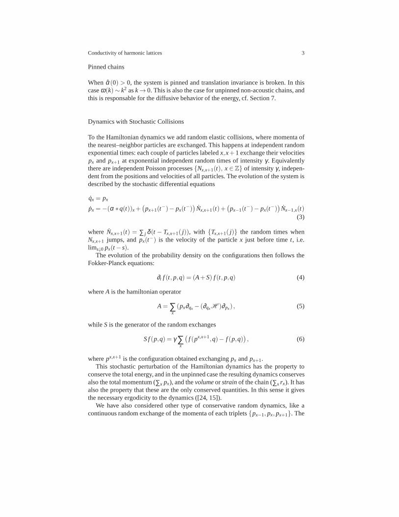
Whenα(0) > 0, the system is pinned and translation invariance is broken. In thiscaseω(k)∼ k2 ask→ 0. This is also the case for unpinned non-acoustic chains, andthis is responsable for the diffusive behavior of the energy, cf. Section 7.
Dynamics with Stochastic Collisions
To the Hamiltonian dynamics we add random elastic collisions, where momenta ofthe nearest–neighbor particles are exchanged. This happens at independent randomexponential times: each couple of particles labeledx,x+1 exchange their velocitiespx and px+1 at exponential independent random times of intensityγ. Equivalentlythere are independent Poisson processes{Nx,x+1(t), x∈ Z} of intensityγ, indepen-dent from the positions and velocities of all particles. Theevolution of the system isdescribed by the stochastic differential equations
qx = px
px =−(α ∗q(t))x+(px+1(t
−)− px(t−))
Nx,x+1(t)+(px−1(t
−)− px(t−)
)Nx−1,x(t)
(3)
where Nx,x+1(t) = ∑ j δ (t − Tx,x+1( j)), with {Tx,x+1( j)} the random times whenNx,x+1 jumps, andpx(t−) is the velocity of the particlex just before timet, i.e.lims↓0 px(t − s).
The evolution of the probability density on the configurations then follows theFokker-Planck equations:
∂t f (t, p,q) = (A+S) f (t, p,q) (4)
whereA is the hamiltonian operator
A= ∑x(px∂qx − (∂qxH )∂px) , (5)
while S is the generator of the random exchanges
S f(p,q) = γ ∑x
(f (px,x+1,q)− f (p,q)
), (6)
wherepx,x+1 is the configuration obtained exchangingpx andpx+1.This stochastic perturbation of the Hamiltonian dynamics has the property to
conserve the total energy, and in the unpinned case the resulting dynamics conservesalso the total momentum (∑x px), and thevolumeor strainof the chain (∑x rx). It hasalso the property that these are the only conserved quantities. In this sense it givesthe necessary ergodicity to the dynamics ([24, 15]).
We have also considered other type of conservative random dynamics, like acontinuous random exchange of the momenta of each triplets{px−1, px, px+1}. The

4 Basile, Bernardin, Jara, Komorowski, Olla
intersection of the kinetic energy spherep2x−1+ p2
x+ p2x+1 =C with the planepx−1+
px+ px+1 =C′ gives a one dimensional circle. Then we define a dynamics on thiscircle by a standard Wiener process on the corresponding angle. This perturbationis locally more mixing, but it gives the same results for the macroscopic transport.
Equilibrium stationary measures
Due to the harmonicity of the interactions, the Gibbs equilibrium stationary mea-sures are Gaussians. Positions and momenta are independentand the distributionis parametrized, accordingto teh rules of statistical mechanics, by the temperatureT = β−1 > 0. In the pinned case, they are formally given by
νβ (dq,dp)∼ e−βH (p,q)
Zdqdp.
In the unpinned case, the correct definition should involve the rx variables. Thenthe distribution of therx’s is Gaussian and becomes uncorrelated in the case of thenearest neighbor interaction. Foracoustic unpinned chainsthe Gibbs measures areparameterized by
λ = (β−1(temperature), p(velocity),τ(tension)),
and are given formally by
νλ (dr,dp)∼ e−β [H (p,q)− p∑x px−τ ∑x rx]
Zdrdp. (7)
Non-acoustic chains are tensionless and the equilibrium measures have a differentparametrization, see Section 7.
Macroscopic space-time scales
We will mostly concentrate on the acoustic unpinned case (except Section 7). In thiscase the total hamiltonian can be written as
H (p,q) := ∑x
p2x
2− 1
4 ∑x,x′
αx−x′ (qx−qx′)2 , (8)
whereqx−qx′ = ∑xy=x′+1 ry for x> x′. We define the energy per atom as:
ex(r, p) :=p2
x
2− 1
4 ∑x′
αx−x′(qx−qx′)2. (9)

Conductivity of harmonic lattices 5
There are three conserved (also calledbalanced) fields: the energy∑x ex, themomentum∑x px and the strain∑x rx . We want to study the macroscopic evolutionof the spatial distribution of these fields in a large space-time scale. We introducea scale parameterε > 0 and, for any smooth test functionJ : R → R, define theempirical distribution
ε ∑x
J(εx)Ux(ε−at), Ux = (rx, px,ex). (10)
We are interested in the limit asε → 0. The parametera∈ [1,2] corresponds todifferent possible scalings. The valuea= 1 corresponds to the hyperbolic scaling,while a= 2 corresponds to the diffusive scaling. The intermediate values 1< a< 2pertain to the superdiffusive scales.
The interest of the unpinned model is that there are three different macroscopicspace-scales where we observe non-trivial behaviour of thechain:a= 1, 3
2,2.
2 Hyperbolic scaling: the linear wave equation.
Let us assume that the dynamics starts with a random initial distributionµε = 〈·〉εof finite energy of sizeε−1, i.e. for some positive constantE0:
ε ∑x〈ex(0)〉ε ≤ E0. (11)
where we denoteex(t) = ex(p(t),q(t)). We will also assume that some smoothmacroscopic initial profiles
u0(y) = (r0(y),p0(y),e0(y))
are associated with the initial distribution, in the sense that:
limε→0
µε
(∣∣∣∣ε ∑x
J(εx)Ux(0)−∫
J(y)u0(y)dy
∣∣∣∣> δ)= 0, ∀δ > 0, (12)
for any test functionJ.Then it can be proven ([28]) that these initial profiles are governed by the linear
wave equation in the following sense
limε→0
ε ∑x
J(εx)Ux(ε−1t) =∫
J(y)u(y, t)dy (13)
whereu(y, t) = (r(y, t),p(y, t),e(y, t)) is the solution of:
∂tr= ∂yp, ∂tp= τ1∂yr, ∂te= τ1∂y(pr) (14)

6 Basile, Bernardin, Jara, Komorowski, Olla
with τ1 =α ′′(0)8π2 (the square of the speed of sound of the chain). Notice that inthe
non-acoustic caseα ′′(0) = 0, there is no evolution at the hyperbolic scale.Observe that the evolution of the fields of strainr and momentump is au-
tonomous of the energy field. Furthermore we can define the macroscopicmechan-ical energy as
emech(y, t) =12
(τ1r(y, t)
2+ p(y, t)2) (15)
and the temperature profile orthermalenergy as
T(y, t) = e(y, t)− emech(y, t). (16)
It follows immediately from (14) thatT(y, t) = T(y,0), i.e. the temperature profiledoes not change on the hyperbolic space-time scale.
There is a corresponding decomposition of the energy of the random initial con-figurations: long wavelengths (invisible for the exchange noise in the dynamics)contribute to the mechanical energy and they will evolve in this hyperbolic scalefollowing the linear equations (14). This energy will eventually disperse to infin-ity at large time (in this scale). Because of the noise dynamics, short wavelengthwill contribute to the variance (temperature) of the distribution, and the correpond-ing profile does not evolve in this hyperbolic scale. See [28]for the details of thisdecomposition.
3 Superdiffusive evolution of the temperature profile.
As we have seen in the previous section, for acoustic chains the mechanical part ofthe energy evolves ballistically in the hyperbolic scale and eventually it will disperseto infinity. Consequently when we look at the larger superdiffusive time scaleε−at,a> 1, we start only with the thermal profile of energy, while the strain and momen-tum profiles are equal to 0. It turns out that, for acoustic chains, the temperatureprofile evolves at the time scale correspondig toa= 3/2:
limε→0
ε ∑x
J(εx) 〈ex(ε−3/2t)〉ε =
∫J(y)T(y, t)dy, t > 0, (17)
whereT(y, t) solves the fractional heat equation
∂tT=−c|∆y|3/4T, T(y,0) = T(y,0) (18)
wherec = α ′′(0)3/42−9/4(3γ)−1/2. This is proven in [27]. We also have that theprofiles for the other conserved quantities remain flat:
Conductivity of harmonic lattices 7
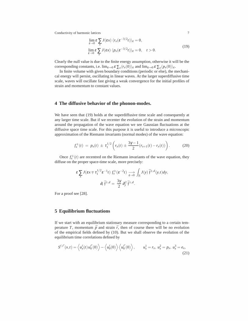
limε→0
ε ∑x
J(εx) 〈rx(ε−3/2t)〉ε = 0,
limε→0
ε ∑x
J(εx) 〈px(ε−3/2t)〉ε = 0, t > 0.(19)
Clearly the null value is due to the finite energy assumption,otherwise it will be thecorresponding constants, i.e. limε→0 ε ∑x〈rx(0)〉ε and limε→0 ε ∑x〈px(0)〉ε .
In finite volume with given boundary conditions (periodic orelse), the mechani-cal energy will persist, oscillating in linear waves. At thelarger superdiffusive timescale, waves will oscillate fast giving a weak convergence for the initial profiles ofstrain and momentum to constant values.
4 The diffusive behavior of the phonon-modes.
We have seen that (19) holds at the superdiffusive time scaleand consequently atany larger time scale. But if we recenter the evolution of thestrain and momentumaround the propagation of the wave equation we see Gaussian fluctuations at thediffusive space time scale. For this purpose it is useful to introduce a microscopicapproximation of the Riemann invariants (normal modes) of the wave equation:
f±x (t) = px(t) ± τ1/21
(rx(t) ±
3γ −12
(rx+1(t)− rx(t))
). (20)
Once f±x (t) are recentred on the Riemann invariants of the wave equation, theydiffuse on the proper space-time scale, more precisely:
ε ∑x
J(εx∓ τ1/21 ε−1t) f±x (ε−2t) −→
ε→0
∫
R
J(y) f±,d(y, t)dy,
∂t f±,d =
3γ2
∂ 2y f±,d.
For a proof see [28].
5 Equilibrium fluctuations
If we start with an equilibrium stationary measure corresponding to a certain tem-peratureT, momentum ¯p and strain ¯r, then of course there will be no evolutionof the empirical fields defined by (10). But we shall observe the evolution of theequilibrium time correlations defined by
Sℓ,ℓ′(x, t) =
⟨uℓx(t)uℓ
′0 (0)
⟩−⟨
uℓ0(0)⟩⟨
uℓ′
0 (0)⟩, u1
x = rx, u2x = px, u3
x = ex,
(21)

8 Basile, Bernardin, Jara, Komorowski, Olla
where〈·〉 denotes the expectation with respect to the dynamics in the correspondingequilibrium. Let us assume for simplicity of notation that ¯r = 0= p, otherwise wehave to shiftx along the characteristics of the linear wave equation. At timet = 0, itis easy to compute the limit (in a distributional sense):
limε→0
ε−1/2S([ε−1y],0) = δ (y)
T 0 αT0 T 0
αT 0 (12 +α2)T2
(22)
whereα is a constant depending only on the interaction.In the hyperbolic time scalea = 1 this correlation matrix evolves deterministi-
cally, i.e.limε→0
ε−1/2S([ε−1y],ε−1t) = S(y, t) (23)
where∂t S
11(y, t) = ∂yS22(y, t), ∂t S
22(y, t) = τ1∂yS11(y, t), (24)
while for the energy correlations
∂t S33(y, t) = 0. (25)
In particular if p= r = 0, energy fluctuations do not evolve at the hyperbolic timescale. As for the energy profile out of equilibrium, the evolution is at a further timescale. By a duality argument (cf. [27]), the evolution of theenergy correlations oc-curs at the superdiffusive time scale witha= 3/2, namely
limε→0
ε−1/2S33([ε−1y],ε−3/2t) = S33(y, t), (26)
whereS33(y, t) is the solution of:
∂tS33 =−c|∆y|3/4S33. (27)
6 The phonon Boltzmann equation
A way to understand the energy superdiffusion in the one-dimensional system is toanalyze its kinetic limit, i.e. a limit for weak noise where the number of stochasticcollisions per unit time remains bounded. In the non-linearcase it corresponds toa weak non-linearity limit as proposed first in his seminal paper [42] in 1929 byPeierls. He intended to compute thermal conductivity for insulators in analogy withthe kinetic theory of gases. The main idea is that at low temperatures the latticevibrations responsible for the energy transport can be described as a gas of inter-acting particles (phonons) characterized by a wave numberk. The time-dependentdistribution function of phonons solves a Boltzmann type equation. Over the last
Conductivity of harmonic lattices 9
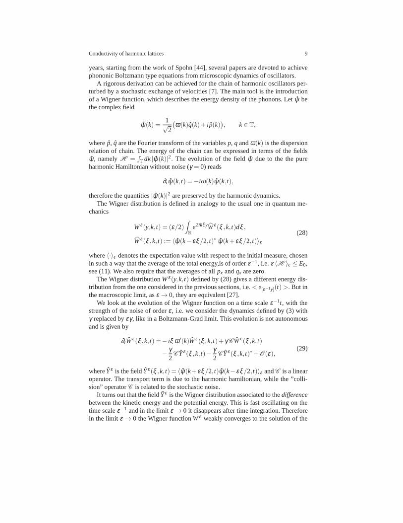
years, starting from the work of Spohn [44], several papers are devoted to achievephononic Boltzmann type equations from microscopic dynamics of oscillators.
A rigorous derivation can be achieved for the chain of harmonic oscillators per-turbed by a stochastic exchange of velocities [7]. The main tool is the introductionof a Wigner function, which describes the energy density of the phonons. Letψ bethe complex field
ψ(k) =1√2
(ω(k)q(k)+ i p(k)
), k∈ T,
wherep, q are the Fourier transform of the variablesp, q andω(k) is the dispersionrelation of chain. The energy of the chain can be expressed interms of the fieldsψ , namelyH =
∫T
dk|ψ(k)|2. The evolution of the fieldψ due to the the pureharmonic Hamiltonian without noise (γ = 0) reads
∂t ψ(k, t) =−iω(k)ψ(k, t),
therefore the quantities|ψ(k)|2 are preserved by the harmonic dynamics.The Wigner distribution is defined in analogy to the usual onein quantum me-
chanics
Wε(y,k, t) = (ε/2)∫
R
e2π iξyWε(ξ ,k, t)dξ ,
Wε(ξ ,k, t) := 〈ψ(k− εξ/2, t)∗ ψ(k+ εξ/2, t)〉ε
(28)
where〈·〉ε denotes the expectation value with respect to the initial measure, chosenin such a way that the average of the total energy,is of orderε−1, i.e.ε 〈H 〉ε ≤ E0,see (11). We also require that the averages of allpx andqx are zero.
The Wigner distributionWε(y,k, t) defined by (28) gives a different energy dis-tribution from the one considered in the previous sections,i.e.< e[ε−1y](t)>. But inthe macroscopic limit, asε → 0, they are equivalent [27].
We look at the evolution of the Wigner function on a time scaleε−1t, with thestrength of the noise of orderε, i.e. we consider the dynamics defined by (3) withγ replaced byεγ, like in a Boltzmann-Grad limit. This evolution is not autonomousand is given by
∂tWε(ξ ,k, t) =− iξ ω ′(k)Wε (ξ ,k, t)+ γ CWε(ξ ,k, t)
− γ2
C Yε(ξ ,k, t)− γ2
C Yε(ξ ,k, t)∗+O(ε),(29)
whereYε is the fieldYε (ξ ,k, t) = 〈ψ(k+εξ/2, t)ψ(k−εξ/2, t)〉ε andC is a linearoperator. The transport term is due to the harmonic hamiltonian, while the ”colli-sion” operatorC is related to the stochastic noise.
It turns out that the fieldYε is the Wigner distribution associated to thedifferencebetween the kinetic energy and the potential energy. This isfast oscillating on thetime scaleε−1 and in the limitε → 0 it disappears after time integration. Thereforein the limit ε → 0 the Wigner functionWε weakly converges to the solution of the

10 Basile, Bernardin, Jara, Komorowski, Olla
following linear Boltzmann equation
∂tW(y,k, t)+1
2πω ′(k)∂yW(y,k, t) = CW(y,k, t). (30)
It describes the evolution of the energy density distribution, over the physical spaceR, of the phonons, characterized by a wave numberk and traveling with velocityω ′(k). We remark that for the unpinned acoustic chainsω ′(k) remains strictly posi-tive for smallk. The collision term has the following expression
C f (k) =∫
T
dk′R(k,k′)[ f (k′)− f (k)],
where the kernelR is positive and symmetric. One can write an exact expressiononR, nevertheless its crucial feature is thatR behaves likek2 for small k, due to thefact that the noise preserves the total momentum. Naıvely,it means that phononswith small wave numbers travel with a finite velocity, but they have low probabil-ity to be scattered, thus their mean free paths have a macroscopic length (ballistictransport). This intuitive picture has an exact statement in the probabilistic interpre-tation of (30). The equation describes the evolution of the probability density of aMarkov process(K(t),Y(t)) onT×R, whereK(t) is a reversible jump process andY(t) is an additive functional ofK, namelyY(t) =
∫ t0 ω ′(Ks)ds. A phonon with the
wave numberk waits in its state an exponentially distributed random timeτ(k) withmean value∼ k−2 for small k. Then it jumps to another statek′ with probability∼ k′2dk′. The additive functionalY(t) describes the position of the phonon and canbe expressed as
Y(t) =Nt
∑i=1
τ(Xi)ω ′(Xi),
where{Xi}i≥1 is the Markov chain given by the sequence of the states visited bythe processK(t). HereNt denotes the number of jumps up to the timet. The taildistribution of the random variables{τ(Xi)ω ′(Xi)} with respect to the stationarymeasureπ of the chain behaves like
π[|τ(Xi)ω ′(Xi)|> λ
]∼ 1
λ 3/2.
Therefore the variablesτ(Xi)ω ′(Xi) have an infinite variance with respect to thestationary measure. We remark that the variance is exactly the expression of thethermal conductivity obtained in [3]. The rescaled processN−2/3Y(Nt) convergesin distribution to a stable symmetric Levy process with index 3/2 ([26], [4]). Asa corollary, the rescaled solution of the Boltzmann equation W(N2/3y,k,Nt) con-verges, asN →+∞, to the solution of the fractional diffusion equation
∂tu(y, t) =−∣∣∆ |3/4u(y, t).
A different, more analytic approach can be found in [39].
Conductivity of harmonic lattices 11
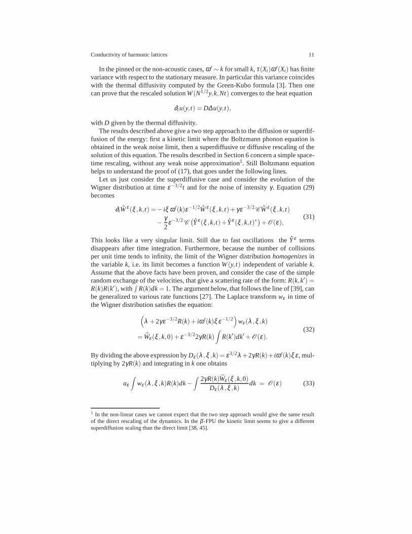
In the pinned or the non-acoustic cases,ω ′ ∼ k for smallk, τ(Xi)ω ′(Xi) has finitevariance with respect to the stationary measure. In particular this variance coincideswith the thermal diffusivity computed by the Green-Kubo formula [3]. Then onecan prove that the rescaled solutionW(N1/2y,k,Nt) converges to the heat equation
∂tu(y, t) = D∆u(y, t),
with D given by the thermal diffusivity.The results described above give a two step approach to the diffusion or superdif-
fusion of the energy: first a kinetic limit where the Boltzmann phonon equation isobtained in the weak noise limit, then a superdiffusive or diffusive rescaling of thesolution of this equation. The results described in Section6 concern a simple space-time rescaling, without any weak noise approximation1. Still Boltzmann equationhelps to understand the proof of (17), that goes under the following lines.
Let us just consider the superdiffusive case and consider the evolution of theWigner distribution at timeε−3/2t and for the noise of intensityγ. Equation (29)becomes
∂tWε(ξ ,k, t) =− iξ ω ′(k)ε−1/2Wε(ξ ,k, t)+ γε−3/2
CWε(ξ ,k, t)
− γ2
ε−3/2C(Yε(ξ ,k, t)+ Yε (ξ ,k, t)∗
)+O(ε),
(31)
This looks like a very singular limit. Still due to fast oscillations theYε termsdisappears after time integration. Furthermore, because the number of collisionsper unit time tends to infinity, the limit of the Wigner distributionhomogenizesinthe variablek, i.e. its limit becomes a functionW(y, t) independent of variablek.Assume that the above facts have been proven, and consider the case of the simplerandom exchange of the velocities, that give a scattering rate of the form:R(k,k′) =R(k)R(k′), with
∫R(k)dk= 1. The argument below, that follows the line of [39], can
be generalized to various rate functions [27]. The Laplace transformwε in time ofthe Wigner distribution satisfies the equation:
(λ +2γε−3/2R(k)+ iω ′(k)ξ ε−1/2
)wε(λ ,ξ ,k)
= Wε(ξ ,k,0)+ ε−3/22γR(k)∫
R(k′)dk′+O(ε).(32)
By dividing the above expression byDε(λ ,ξ ,k) = ε3/2λ +2γR(k)+ iω ′(k)ξ ε, mul-tiplying by 2γR(k) and integrating ink one obtains
aε
∫wε (λ ,ξ ,k)R(k)dk−
∫2γR(k)Wε(ξ ,k,0)
Dε(λ ,ξ ,k)dk = O(ε) (33)
1 In the non-linear cases we cannot expect that the two step approach would give the same resultof the direct rescaling of the dynamics. In theβ -FPU the kinetic limit seems to give a differentsuperdiffusion scaling than the direct limit [38, 45].
12 Basile, Bernardin, Jara, Komorowski, Olla
where, sinceR(k)∼ k2 and due to the assumptions made onω ′(k):
aε = 2γε−3/2(
1−∫
2γR2(k)Dε(λ ,ξ ,k)
dk
)−→ε→0
λ + c|ξ |3/2.
Thanks to the homogenization property ofWε∫
wε (λ ,ξ ,k)R(k)dk −→ε→0
w(λ ,ξ ).
Furthermore2γR(k)
Dε(λ ,ξ ,k)−→ε→0
1,
and we conclude that the limit functionw(λ ,ξ ) satisfies the equation
(λ + c|ξ |3/2
)w(λ ,ξ ) =
∫W(ξ ,k,0)dk (34)
whereW(ξ ,k,0) is the limit of the initial condition. Equation (34) is the Laplace-Fourier transform of the fractional heat equation. Assuming instead thatω ′(k) ∼ k,a similar argument gives the normal heat equation [27].
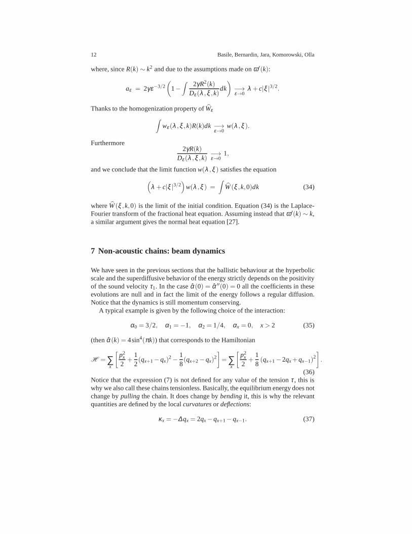
7 Non-acoustic chains: beam dynamics
We have seen in the previous sections that the ballistic behaviour at the hyperbolicscale and the superdiffusive behavior of the energy strictly depends on the positivityof the sound velocityτ1. In the caseα(0) = α ′′(0) = 0 all the coefficients in theseevolutions are null and in fact the limit of the energy follows a regular diffusion.Notice that the dynamics is still momentum conserving.
A typical example is given by the following choice of the interaction:
α0 = 3/2, α1 =−1, α2 = 1/4, αx = 0, x> 2 (35)
(thenα(k) = 4sin4(πk)) that corresponds to the Hamiltonian
H =∑x
[p2
x
2+
12(qx+1−qx)
2− 18(qx+2−qx)
2]=∑
x
[p2
x
2+
18(qx+1−2qx+qx−1)
2].
(36)Notice that the expression (7) is not defined for any value of the tensionτ, this iswhy we also call these chains tensionless. Basically, the equilibrium energy does notchange bypulling the chain. It does change bybendingit, this is why the relevantquantities are defined by the localcurvaturesor deflections:
κx =−∆qx = 2qx−qx+1−qx−1. (37)

Conductivity of harmonic lattices 13
The relevant balanced quantities are now(κx, px,ex).The invariant equilibrium measures are formally given by
e−β [H − p∑x px−L∑x κx]
Zdκ dp (38)
where the parameterL is called load. Notice that these measures would be non-translation invariant in the coordinatesrx’s.
Under these conditions the sound velocityτ1 is always null, and there is no bal-listic evolution of the chain. In fact it turns out that the macroscopic evolution of thethree quantities(k(t,y),p(t,y),e(t,y)) is diffusive. By defining
emech(t,y) =12
(p(t,y)2+
14k2)
and T(t,y) = e(t,y)− emech(t,y),
after the corresponding space-time scaling we obtain ([29]):
∂tk =− ∂ 2y p,
∂tp = 14∂ 2
y k+ γ∂ 2y p,
∂tT = Dγ∂ 2y T+ γ
2
[(∂yp)
2− p∂ 2yp
].
(39)
The first two equations are the damped Euler-Bernoulli beam equations. The thirdone describes the diffusive behavior of the energy. The thermal diffusivity Dγ can becomputed explicitely and diverges asγ → 0 (the deterministic dynamics has ballisticenergy transport as every harmonic chain). (the damping terms involvingγ are dueto the exchange noise). In particular for constant initial values ofk andp, the energy(temperature) profile follows a normal heat equation with the thermal diffusivitythat can be computed explicitly (cf. [29]).
These models provide rigorous counter-examples to the usual conjecture thatthe momentum conservation in one dimension always implies superdiffusivity ofthe energy (cf [34, 20]). The presence of a non-vanishing sound velocity seems anecessary condition.
8 A simpler model with two conserved quantities
In this section we consider the nearest neighbors unpinned harmonic chain (withmass 1 and coupling forcesα1 = α−1 =−α0
2 ) but we add different stochastic colli-sions with the properties that they conserve the total energy and some extra quantity(that we call ”volume”) but no longer momentum and stretch. By defininga=
√α0
and the field{ηx ∈ R ; x∈ Z} by η2x = arx andη2x+1 = px, the Hamiltonian equa-tions are reduced to
ηx = a(ηx+1−ηx−1).

14 Basile, Bernardin, Jara, Komorowski, Olla
The stochastic collisions are such that at random times given by independent Pois-son clocksNx,x+1(t) of intensityγ the kinetic energy at sitex is exchanged with thecorresponding potential energy. The simplest way to do it isto exchange the vari-
ableηx with ηx+1. Because of the form of the noise the total energy∑xη2
x2m and the
”volume” ∑xηx = ∑x(px+arx) are the only conserved quantities of the dynamics([17]). By reducing the number of conserved quantities from3 (energy, momentum,stretch) to 2 (energy, volume) we expect to see easily the influence of the other con-served quantity on the superdiffusion of energy. The natureof the superdiffusionfor models with two conserved quantities are studied in the nonlinear fluctuatinghydrodynamics framework by Spohn and Stoltz in [47].
In the hyperbolic time scaling, starting from an initial distribution associatedto some smooth macroscopic initial volume-energy profiles(v0(y),e0(y)), we canprove that these initial profiles evolve following the linear wave equation(v(t,y),e(t,y))which is solution of
∂tv= 2a∂yv, ∂te= a∂y(v2).
As in Section 2 we can introduce themechanical energyemech(y, t) =v2(y,t)
2 and thethermal energyT(y, t) = e(y, t)− emech(y, t). The later remains constant in time.
Mutatis mutandis the discussion of Sections 3, 4 and 5 can be applied to thismodel with two conserved quantities with very similar conclusions2 ([11, 12]).The interesting difference is that in (18) and (27) the fractional Laplacian has to bereplaced by theskew fractional Laplacian:
∂tT=−c{|∆y|3/4−∇y|∆y|1/4} T, T(y,0) = T(y,0) (40)
for a suitable explicit constantc > 0. The skewness is produced here by the inter-action of the (unique) sound mode with the heat mode. In the models of Section 1which conserve three quantities, there are two sound modes with opposite velocities.The skewness produced by each of them is exactly counterbalanced by the other oneso that it is not seen in the final equations (18) and (27).
The extension problem for the skew–fractional Laplacian
For the model with two conserved quantities introduced in this section, the deriva-tion of the skew fractional heat equation, at least at the level of the fluctuations inequilibrium as defined in Section 5, can be implemented by means of the so-calledextension problemfor the fractional Laplacian [48], [18]. As we will see, thisexten-sion problem does not only provides a different derivation,but it also clarifies therole of the other (fast) conservation law (i.e. the volume).It can be checked that foranyβ > 0 and anyρ ∈ R, the product measure with Gaussian marginals of meanρand variance (temperature)β−1 are stationary under the dynamics of{ηx(t);x∈Z}.Let us assume that the dynamics starts from a stationary state. For simplicity we as-
2 In [11] only the equilibrium fluctuations are considered butthe methods developed in [27], [28]can be applied also to the models considered in this section.

Conductivity of harmonic lattices 15
sumeρ = 0 anda= 1. The space-time energy correlation functionSε(x, t) is definedhere by
Sε(x, t) =⟨(ηx(ε−3/2t)2−β−1)(η0(0)
2−β−1)⟩.
It turns out that the energy fluctuations are driven by volumecorrelations. Thereforeit makes sense to define thevolumecorrelation function as
Gε(x,y, t) =⟨
ηx(ε−3/2t)ηy(ε−3/2t) (η0(0)2−β−1)
⟩.
Let f : [0,T]×R → R be a smooth, regular function and for eacht ∈ [0,T], letut : R×R+ → R be the solution of the boundary-value problem
{−∂xu+ γ∂ 2
y u= 0∂yu(x,0) = ∂x f (x, t).
It turns out that∂xut(x,0) = L ft(x), whereL is the skew fractional Laplaciandefined in (40).
For test functionsf : R→ R andu : R×R+ → R define
〈Sε(t), f 〉ε = ∑x∈Z
Sε(x, t) f (εx),
〈Gε(t),u〉ε = ∑x,y∈Zx<y
Gε(x,y, t) u( ε
2(x+ y),√
ε(y− x)).
After an explicit calculation we have:
ddt
{〈Sε(t) ft 〉ε − ε1/2
2γ 〈Gε(t),ut〉ε + ε〈Sε(t),ut(·,0)〉ε
}= 〈Sε(t),∂x ft〉ε
plus error terms that vanish asε → 0. From this observation it is not very difficultto obtain that, for any smooth functionf of compact support,
limε→0
〈Sε(t), f 〉ε =
∫P(t,x) f (x)dx,
whereP(t,x) is the fundamental solution of the skew fractional heat equation (40).Let us explain in more details why the introduction of the test function ut
solves the equation for the energy correlation functionSε(x, t). It is reasonable toparametrize volume correlations by its distance to the diagonalx = y. The micro-scopic current associated to the energyηx(t)2 is equal toηx(t)ηx+1(t), which can beunderstood as the volume correlations around the diagonalx = y. Volume evolvesin the hyperbolic scale with speed 2. Fluctuations around this transport evolutionappear in the diffusive scale and are governed by a diffusionequation. This meansthat at the hyperbolic scaleε−1, fluctuations are of orderε−1/2, explaining the non-isotropic space scaling introduced in the definition of〈Gε(t),u〉ε . It turns out thatthe couple(Sε ,Gε) satisfies a closed system of equations, which can be checked tobe a semidiscrete approximation of the system

16 Basile, Bernardin, Jara, Komorowski, Olla
√ε∂tut =−∂xut + γ∂ 2
y ut
∂yut(x,0) = ∂x ft (x)∂t ft = ∂xut(x,0).
Therefore, the volume serves as a fast variable for the evolution of the energy, whichcorresponds to a slow variable. The extension problem playsthe role of the cellproblem for the homogenization of this fast-slow system of evolutions.
9 The dynamics in higher dimension
One of the interesting features of the harmonic dynamics with energy and momen-tum conservative noise is that they reproduce, at least qualitatively, the expectedbehavior of the non-linear dynamics, also in higher dimensions. In particular in thethree or higher dimension the thermal conductivity, computed by the Green-Kuboformula, is finite, while it diverges logarithmically in twodimension (always fornon-acoustic systems), cf. [2, 3].
In dimensiond ≥ 3 it can be also proven that equilibrium fluctuations evolvediffusively, i.e. that the asymptotic correlationS33(y, t), defined in section 7 but witha diffusive scaling, satisfies [5]:
∂t S33= D∂ 2
y S33 (41)
whereD can be computed explicitely by Green-Kubo formula in terms of ω andscattering rateR [2, 3]. Similar finite diffusivity and diffusive evolution of the fluc-tuations are proven for pinned models (α(0)> 0), see [5]. In two dimensions, whilethe logarithmic divergence of the Green-Kubo expression ofthe thermal conductiv-ity is proven in [3], the corresponding diffusive behaviourat the logarithmic cor-rected time scale is still an open problem. For the result obtained from the kineticequation see [8]. The two-dimensional model is particularly interesting in light ofthe large thermal conductivity measured experimentally ongraphene [51], an essen-tially a two-dimensional material.
10 Thermal boundary conditions and the non-equilibriumstationary states
Traditionally the problem of thermal conductivity has beenapproached by consid-ering the stationary non-equilibrium state for a finite system in contact with heatbath at different temperatures (cf.[43, 34]). This set-up is particularly suitable fornumerical simulations and convenient because it gives an straight operational defi-nition of the thermal conductivity in terms of the stationary flux of energy, avoidingto specify the macroscopic evolution equation. But for the theoretical understanding

Conductivity of harmonic lattices 17
and corresponding mathematical proofs of the thermal conductivity phenomena, thisis much harder than the non-stationary approach described in the previous section.This because the stationary state conceals the space-time scale.
The finite system consists of 2N+1 atoms, labelled byx=−N, . . . ,N, with endpoints connected to two heat baths at temperatureTl andTr . These baths are modeledby Langevin stochastic dynamics, so that the evolution equations are given by
qx = px, x=−N, . . . ,N,
px =−(αN ∗q(t))x+(px+1(t
−)− px(t−)
)Nx,x+1(t)+
(px−1(t
−)− px(t−)
)Nx−1,x(t)
+ δx,−N
(−p−N+
√2Tl dw−N(t)
)+ δx,N
(−pN +
√2Tr dwN(t)
),
(42)
wherew−N(t),wN(t) are two independent standard Brownian motions, and the cou-pling αN is properly defined in order to take into account the boundaryconditions.For this finite dynamics there is a (non-equilibrium) uniquestationary state, wherethe energy flow from the hot to the cold side. Observe that because of the exchangenoise between the atoms, the stationary state is not Gaussian, unlike in the casestudied in [43].
Denoting the stationary energy flux byJN, the thermal conductivity of the finitechain is defined as
κN = lim|Tl−Tr |→0
(2N+1)JN
Tl −Tr. (43)
For a finiteN it is not hard to prove thatκN can be expressed in terms of the cor-responding Green-Kubo formula. For the periodic boundary unpinned acoustic casethis identification givesκN ∼ N1/2 (cf. [2]). For the noise that conserves only theenergy, but not momentum (like independent random flips of the signs of the mo-menta), the system has a finite thermal diffusivity and the limit κN → κ , asN→+∞,can be computed explicitely, as proven in [14].
The natural question is about the macroscopic evolution of the temperature pro-file in a non-stationary situation, and the corresponding stationary profile. It turnsout that this macroscopic equation is given by a fractional heat equation similar to(17) with a proper definition of the fractional laplacian|∆ |3/4 on the interval[−1,1]subject to the boundary conditionsT(−1) = Tl ,T(1) = Tr . This is defined by usingthe following orthonormal basis of functions on the interval [−1,1]:
un(y) = cos(nπ(y+1)/2), n= 0,1, . . . (44)
Any continuos functionf (y) on [−1,1] can be expressed in terms of a series ex-pansion inun. Then we define|∆ |sun(y) = (nπ/2)2sun(y). Observe that fors= 1we recover the usual definition of the Laplacian. Fors 6= 1 this isnot equivalent toother definitions of the fractional Laplacian in a bounded interval, e.g. [52].
Correspondingly the stationary profile is given by
18 Basile, Bernardin, Jara, Komorowski, Olla
|∆ |sT= 0, in (−1,1)
T(−1) = Tl , T(1) = Tr ,(45)
namelyT(y) = 12(Tl +Tr)+
12(Tl −Tr)θ (y), with
θ (y) = cs ∑modd
1m2s cos
(mπ(y+1)/2
),
cs such thatθ (−1) = 1. This expression corresponds with the formula computeddirectly in [36] using a continuous approximation of the covariance matrix of thestationary state for the dynamics with fixed boundaries.
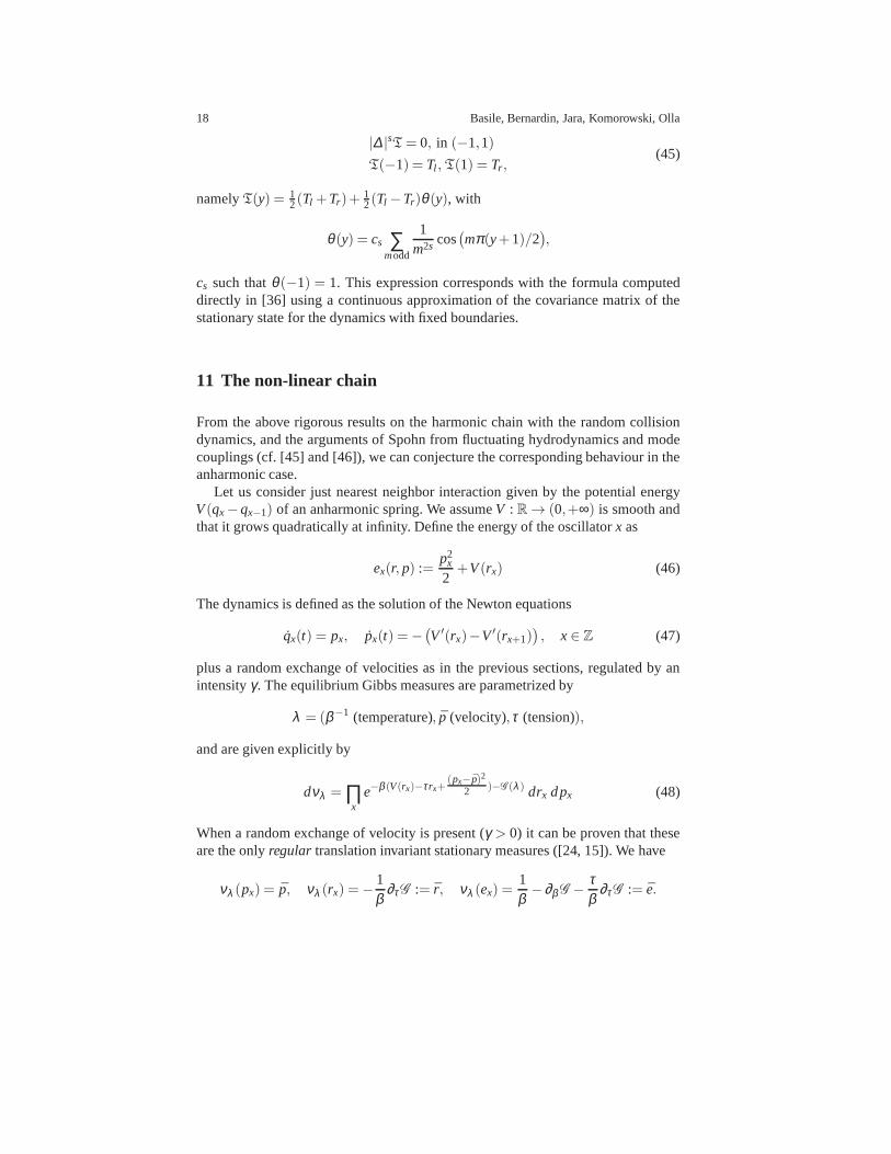
11 The non-linear chain
From the above rigorous results on the harmonic chain with the random collisiondynamics, and the arguments of Spohn from fluctuating hydrodynamics and modecouplings (cf. [45] and [46]), we can conjecture the corresponding behaviour in theanharmonic case.
Let us consider just nearest neighbor interaction given by the potential energyV(qx−qx−1) of an anharmonic spring. We assumeV : R→ (0,+∞) is smooth andthat it grows quadratically at infinity. Define the energy of the oscillatorx as
ex(r, p) :=p2
x
2+V(rx) (46)
The dynamics is defined as the solution of the Newton equations
qx(t) = px, px(t) =−(V ′(rx)−V′(rx+1)
), x∈ Z (47)
plus a random exchange of velocities as in the previous sections, regulated by anintensityγ. The equilibrium Gibbs measures are parametrized by
λ = (β−1 (temperature), p (velocity),τ (tension)),
and are given explicitly by
dνλ = ∏x
e−β (V(rx)−τrx+(px− p)2
2 )−G (λ ) drx dpx (48)
When a random exchange of velocity is present (γ > 0) it can be proven that theseare the onlyregular translation invariant stationary measures ([24, 15]). We have
νλ (px) = p, νλ (rx) =− 1β
∂τG := r, νλ (ex) =1β− ∂β G − τ
β∂τG := e.
Conductivity of harmonic lattices 19
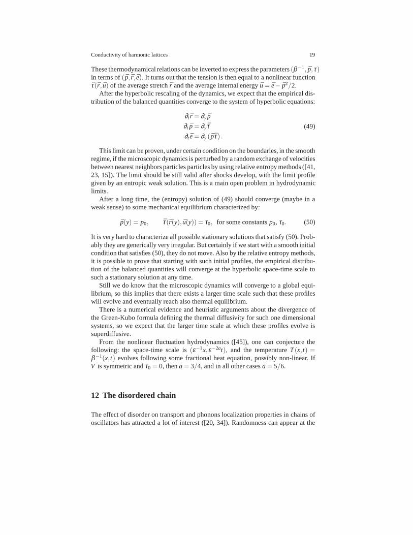
These thermodynamical relations can be inverted to expressthe parameters(β−1, p,τ)in terms of(p, r, e). It turns out that the tension is then equal to a nonlinear functionτ(r , u) of the average stretch ¯r and the average internal energy ¯u= e− p2/2.
After the hyperbolic rescaling of the dynamics, we expect that the empirical dis-tribution of the balanced quantities converge to the systemof hyperbolic equations:
∂t r = ∂y p
∂t p= ∂yτ∂t e= ∂y (pτ) .
(49)
This limit can be proven, under certain condition on the boundaries, in the smoothregime, if the microscopic dynamics is perturbed by a randomexchange of velocitiesbetween nearest neighbors particles particles by using relative entropy methods ([41,23, 15]). The limit should be still valid after shocks develop, with the limit profilegiven by an entropic weak solution. This is a main open problem in hydrodynamiclimits.
After a long time, the (entropy) solution of (49) should converge (maybe in aweak sense) to some mechanical equilibrium characterized by:
p(y) = p0, τ(r(y), u(y)) = τ0, for some constantsp0, τ0. (50)
It is very hard to characterize all possible stationary solutions that satisfy (50). Prob-ably they are generically very irregular. But certainly if we start with a smooth initialcondition that satisfies (50), they do not move. Also by the relative entropy methods,it is possible to prove that starting with such initial profiles, the empirical distribu-tion of the balanced quantities will converge at the hyperbolic space-time scale tosuch a stationary solution at any time.
Still we do know that the microscopic dynamics will convergeto a global equi-librium, so this implies that there exists a larger time scale such that these profileswill evolve and eventually reach also thermal equilibrium.
There is a numerical evidence and heuristic arguments aboutthe divergence ofthe Green-Kubo formula defining the thermal diffusivity forsuch one dimensionalsystems, so we expect that the larger time scale at which these profiles evolve issuperdiffusive.
From the nonlinear fluctuation hydrodynamics ([45]), one can conjecture thefollowing: the space-time scale is(ε−1x,ε−2at), and the temperatureT(x, t) =β−1(x, t) evolves following some fractional heat equation, possiblynon-linear. IfV is symmetric andτ0 = 0, thena= 3/4, and in all other casesa= 5/6.
12 The disordered chain
The effect of disorder on transport and phonons localization properties in chains ofoscillators has attracted a lot of interest ([20, 34]). Randomness can appear at the
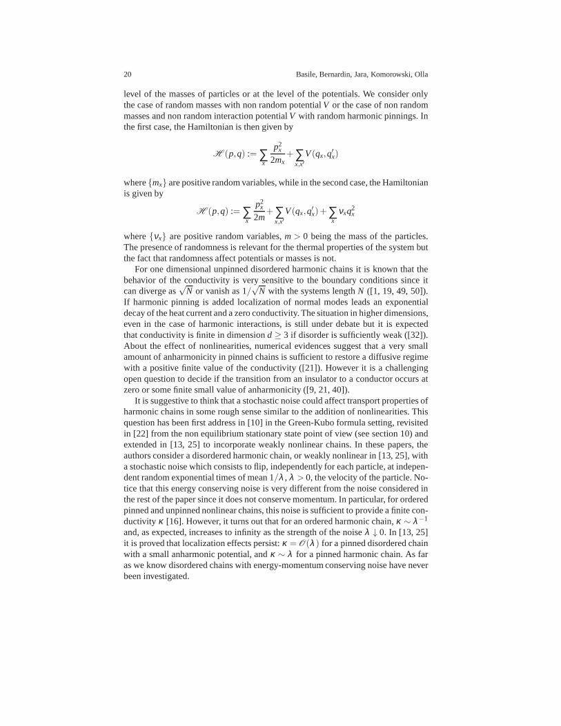
20 Basile, Bernardin, Jara, Komorowski, Olla
level of the masses of particles or at the level of the potentials. We consider onlythe case of random masses with non random potentialV or the case of non randommasses and non random interaction potentialV with random harmonic pinnings. Inthe first case, the Hamiltonian is then given by
H (p,q) := ∑x
p2x
2mx+∑
x,x′V(qx,q
′x)
where{mx} are positive random variables, while in the second case, theHamiltonianis given by
H (p,q) := ∑x
p2x
2m+∑
x,x′V(qx,q
′x)+∑
xνxq
2x
where{νx} are positive random variables,m> 0 being the mass of the particles.The presence of randomness is relevant for the thermal properties of the system butthe fact that randomness affect potentials or masses is not.
For one dimensional unpinned disordered harmonic chains itis known that thebehavior of the conductivity is very sensitive to the boundary conditions since itcan diverge as
√N or vanish as 1/
√N with the systems lengthN ([1, 19, 49, 50]).
If harmonic pinning is added localization of normal modes leads an exponentialdecay of the heat current and a zero conductivity. The situation in higher dimensions,even in the case of harmonic interactions, is still under debate but it is expectedthat conductivity is finite in dimensiond ≥ 3 if disorder is sufficiently weak ([32]).About the effect of nonlinearities, numerical evidences suggest that a very smallamount of anharmonicity in pinned chains is sufficient to restore a diffusive regimewith a positive finite value of the conductivity ([21]). However it is a challengingopen question to decide if the transition from an insulator to a conductor occurs atzero or some finite small value of anharmonicity ([9, 21, 40]).
It is suggestive to think that a stochastic noise could affect transport properties ofharmonic chains in some rough sense similar to the addition of nonlinearities. Thisquestion has been first address in [10] in the Green-Kubo formula setting, revisitedin [22] from the non equilibrium stationary state point of view (see section 10) andextended in [13, 25] to incorporate weakly nonlinear chains. In these papers, theauthors consider a disordered harmonic chain, or weakly nonlinear in [13, 25], witha stochastic noise which consists to flip, independently foreach particle, at indepen-dent random exponential times of mean 1/λ , λ > 0, the velocity of the particle. No-tice that this energy conserving noise is very different from the noise considered inthe rest of the paper since it does not conserve momentum. In particular, for orderedpinned and unpinned nonlinear chains, this noise is sufficient to provide a finite con-ductivity κ [16]. However, it turns out that for an ordered harmonic chain, κ ∼ λ−1
and, as expected, increases to infinity as the strength of thenoiseλ ↓ 0. In [13, 25]it is proved that localization effects persist:κ =O(λ ) for a pinned disordered chainwith a small anharmonic potential, andκ ∼ λ for a pinned harmonic chain. As faras we know disordered chains with energy-momentum conserving noise have neverbeen investigated.

Conductivity of harmonic lattices 21
Acknowledgements We thank Herbert Spohn for many inspiring discussions on this subject.The research of Cedric Bernardin was supported in part by the French Ministry of Education
through the grant ANR-EDNHS. The work of Stefano Olla has been partially supported by theEuropean Advanced GrantMacroscopic Laws and Dynamical Systems(MALADY) (ERC AdG246953) and by a CNPq grantSciences Without Frontiers. Tomasz Komorowski acknowledges thesupport of the Polish National Science Center grant UMO-2012/07/B/SR1/03320.
References
1. O. Ajanki, F. Huveneers, Rigorous scaling law for the heatcurrent in disordered harmonicchain Commun. Math. Phys.30184183 (2011).
2. G. Basile, C. Bernardin, S. Olla, A momentum conserving model with anomalous thermalconductivity in low dimension, Phys. Rev. Lett.96, 204303 (2006), DOI 10.1103/Phys-RevLett.96.204303.
3. G. Basile, C. Bernardin, S. Olla, Thermal Conductivity for a Momentum Conservative Model,Comm. Math. Phys.287, 67–98, (2009).
4. G. Basile, A. Bovier, Convergence of a kinetic equation toa fractional diffusion equation,Markov Proc. Rel. Fields16, 15-44 (2010);
5. G. Basile, S. Olla, Energy Diffusion in Harmonic System with Conservative Noise, J. Stat.Phys.,155, no. 6, 1126-1142, (2014), (DOI) 10.1007/s10955-013-0908-4.
6. G. Basile, T. Komorowski, S. Olla, Temperature profile evolution in a one dimensional chainwith boundary thermal conditions, in preparation.
7. G. Basile, S. Olla, H. Spohn, Energy transport in stochastically perturbed lattice dynamics,Arch.Rat.Mech.,195, no. 1, 171-203, (2009).
8. G. Basile, From a kinetic equation to a diffusion under an anomalous scaling. Ann. Inst. H.Poincare Prob. Stat.,50, No. 4, 1301–1322 (2014), DOI: 10.1214/13-AIHP554.
9. D.M. Basko, Weak chaos in the disordered nonlinear Schrodinger chain: destruction of An-derson localization by Arnold diffusion, Ann. Phys.3261577655, (2011).
10. C. Bernardin, Thermal conductivity for a noisy disordered harmonic chain, J. Stat. Phys.133(3), 417433 (2008).
11. C. Bernardin, P. Goncalves, M. Jara, 3/4 Fractional superdiffusion of energy in a system ofharmonic oscillators perturbed by a conservative noise, arxiv.org/abs/1402.1562v3, to appearin Arch. Rational Mech. Anal. 2015.
12. C. Bernardin, P. Goncalves, M. Jara, M. Sasada, M. Simon.From normal diffusion to su-perdiffusion of energy in the evanescent flip noise limit. J.Stat. Phys.159, no. 6, 13271368(2015).
13. C. Bernardin, F. Huveneers, Small perturbation of a disordered harmonic chain by a noise andan anharmonic potential, Probab. Theory Related Fields157, no. 1-2, 301331 (2013).
14. C. Bernardin, S. Olla, Fourier law and fluctuations for a microscopic model of heat conduc-tion, J. Stat.Phys.,118, nos.3/4, 271-289, (2005).
15. C. Bernardin, S. Olla, Thermodynamics and non-equilibrium macroscopicdynamics of chains of anharmonic oscillators, Lecture Notes available athttps://www.ceremade.dauphine.fr/ olla/ (2014),
16. C. Bernardin, S. Olla, Transport Properties of a Chain ofAnharmonic Oscillators with randomflip of velocities, Journal of Statistical Physics145, 1224-1255, (2011).
17. C. Bernardin, G. Stoltz, Anomalous diffusion for a classof systems with two conserved quan-tities, Nonlinearity25, N. 4, 1099-1133 (2012).
18. L. Caffarelli, L. Silvestre: An extension problem related to the fractional Laplacian. Commun.Partial Differ. Equations32(8), 1245-1260 (2007).
19. A. Casher, J.L. Lebowitz, Heat flow in regular and disordered harmonic chains,J.Math.Phys.12 170111 (1971).

22 Basile, Bernardin, Jara, Komorowski, Olla
20. A. Dhar, Heat Transport in Low Dimensional Systems, Adv.In Phys.57, 5, 457-537, (2008).21. A. Dhar and J.L. Lebowitz, Effect of phonon-phonon interactions on localization
Phys.Rev.Lett.100134301 (2008).22. A. Dhar, K. Venkateshan, J.L. Lebowitz, Heat conductionin disordered harmonic lattices with
energy- conserving noise. Phys. Rev. E83(2), 021108 (2011).23. N. Even, S. Olla, Hydrodynamic Limit for an Hamiltonian System with Boundary Conditions
and Conservative Noise, Arch.Rat.Mech.Appl.,213, 561-585, (2014). DOI 10.1007/s00205-014-0741-1
24. J. Fritz, T. Funaki, J.L. Lebowitz, Stationary states ofrandom Hamiltonian systems, Probab.Theory Related Fields,99 , 211–236 (1994).
25. F. Huveneers, Drastic fall-off of the thermal conductivity for disordered lattices in the limitof weak anharmonic interactions, Nonlinearity26, no. 3, 837854 (2013).
26. M. Jara, T. Komorowski, S. Olla, A limit theorem for an additive functionals of Markovchains, Annals of Applied Probability19, No. 6, 2270-2300, (2009).
27. M. Jara, T. Komorowski, S. Olla, Superdiffusion of Energy in a Chain of harmonic Oscillatorswith Noise, Commun. Math. Phys.339, 407–453 (2015), (DOI) 10.1007/s00220-015-2417-6.
28. T. Komorowski, S. Olla, Ballistic and superdiffusive scales in macroscopic evolution of achain of oscillators, arXiv:1506.06465, (2015).
29. T. Komorowski, S. Olla, Diffusive propagation of energyin a non-acoustic chain, in prepara-tion.
30. T. Komorowski, S. Olla, L. Ryzhik, Asymptotics of the solutions of the stochastic lattice waveequation, Arch. Rational Mech. Anal.,209, 455-494, 2013.
31. T. Komorowski, L. Stepien, Long time, large scale limit of the Wigner transform for a systemof linear oscillators in one dimension, Journ. Stat. Phys.,Vol. 148, pp 1-37 (2012).
32. A. Kundu, A. Chaudhuri, D. Roy, A. Dhar, J.L. Lebowitz, H.Spohn, Heat transport andphonon localization in mass-disordered harmonic crystals, Phys. Rev. B81064301, 2010
33. O. Lanford, J.L. Lebowitz, E. Lieb, Time Evolution of Infinite Anharmonic Systems, J. Stat.Phys.16, n. 6, 453-461, (1977).
34. S. Lepri, R. Livi, A. Politi, Thermal Conduction in classical low-dimensional lattices, Phys.Rep.377, 1-80 (2003).
35. S. Lepri, R. Livi, A. Politi, Heat conduction in chains ofnonlinear oscillators, Phys. Rev. Lett.78, 1896 (1997).
36. S. Lepri, C. Meija-Monasterio, A. Politi, A stochastic model of anomalous heat transport:analytical solution of the steady state, J. Phys. A: Math. Gen. 42, (2009) 025001.
37. Lukkarinen, J., Spohn, H. (2006). Kinetic Limit for WavePropagation in a Random Medium.Arch. for Rat. Mech. and Anal.,183, 1, 93-162.
38. Lukkarinen, J. and Spohn, H., Anomalous energy transport in the FPU-β chain. Comm. PureAppl. Math., 61: 1753–1786, (2008). doi: 10.1002/cpa.20243
39. A. Mellet, S. Mischler, C. Mouhot, Fractional diffusionlimit for collisional kinetic equations,Arch. for Rat. Mech. and Anal.199, 2, pp 493-525 (2011)
40. V. Oganesyan, A. Pal, D. Huse, Energy transport in disordered classical spin chains,Phys.Rev.B80, 115104 (2009).
41. S. Olla, S.R.S. Varadhan, H. T. Yau, Hydrodynamic Limit for a Hamiltonian System withWeak Noise, Comm. Math. Phys.155, 523-560, 1993.
42. R. E. Peierls, Zur kinetischen Theorie der Waermeleitung in Kristallen, Ann. Phys. Lpz.3,1055-1101, (1929).
43. Z. Rieder, J.L. Lebowitz, E. Lieb, Properties of harmonic crystal in a stationary non-equilibrium state, J. Math. Phys.8, 1073-1078 (1967).
44. H. Spohn The phonon Boltzmann equation, properties and link to weakly anharmonic latticedynamics, J. Stat. Phys.124, no. 2-4, 1041-1104, (2006).
45. H. Spohn, Nonlinear fluctuating hydrodynamics for anharmonic chains, J. Stat. Phys.154no.5, 1191-1227, (2014).
46. H. Spohn, Fluctuating hydrodynamics approach to equilibrium time correlations for anhar-monic chains, this issue.

Conductivity of harmonic lattices 23
47. H. Spohn, G. Stoltz, Nonlinear fluctuating hydrodynamics in one dimension: the case of twoconserved fields, J. Stat. Phys.,160, 861–884 (2015), DOI 10.1007/s10955-015-1214-0.
48. D. W. Stroock, S.R.S. Varadhan, Diffusion Processes with Boundary Conditions, Comm. PureAppl. Math.24, 147-225 (1971).
49. R.J. Rubin, W.L. Greer, Abnormal lattice thermal conductivity of a one-dimensional, har-monic, isotopically disordered crystal, J. Math. Phys.121686701 (1971).
50. T. Verheggen, Transmission coefficient and heat conduction of a harmonic chain with randommasses: asymptotic estimates on products of random matrices, Commun. Math. Phys.68, 69–82 (1979).
51. Y.Xu, Z. Li, W. Duan, Thermal and Thermoelectric Properties of Graphene, Small 2014,10,No. 11, 21822199, DOI: 10.1002/smll.201303701.
52. A. Zola, A. Rosso, M. Kardar, Fractional Laplacian in a Bounded Interval, Phys. Rev. E76,21116 (2007).