NCAR/TN-344+IANCAR TECHNICAL NOTE

November 1989

Theory and Application ofNonlinear Normal Mode Initialization

RONALD M. ERRICO

1210

Us

C3

zLJen

0

COc-

0

LI

V)

1010

10

10

10

8

6

4

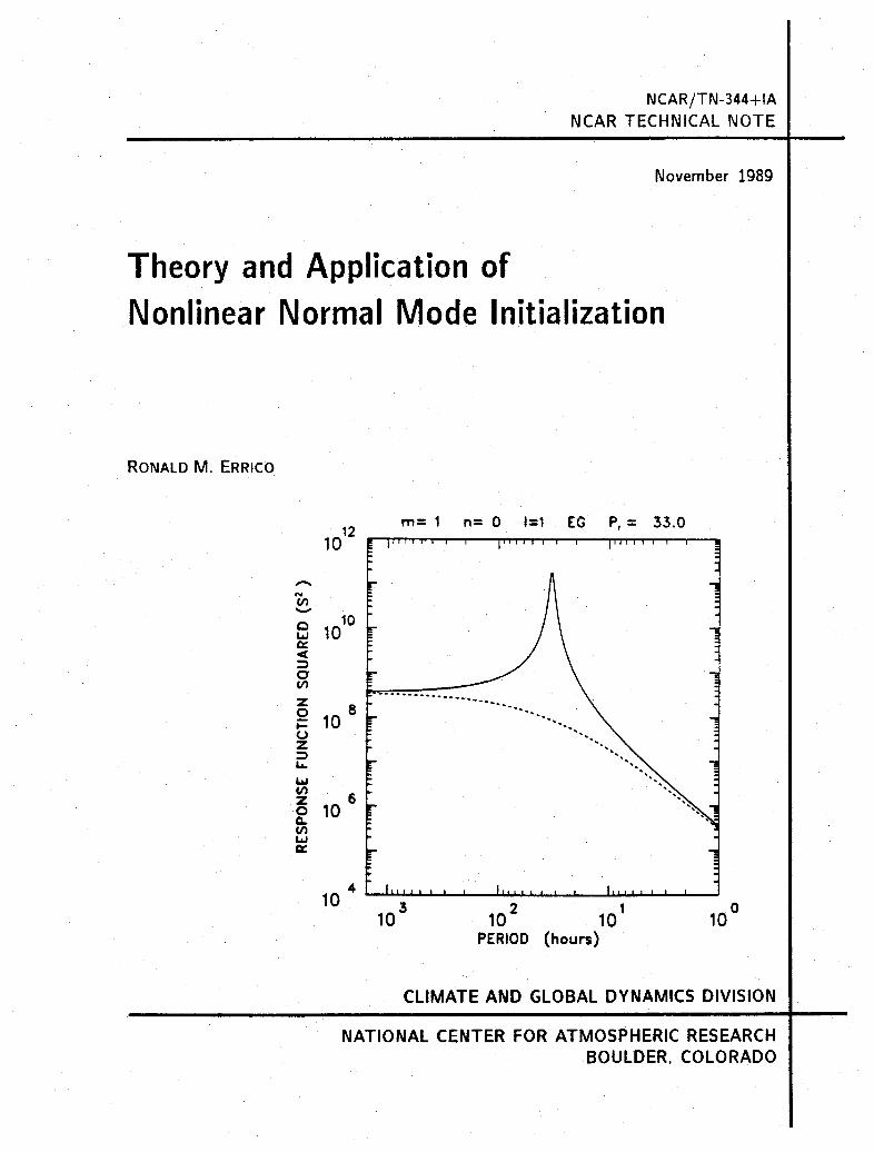
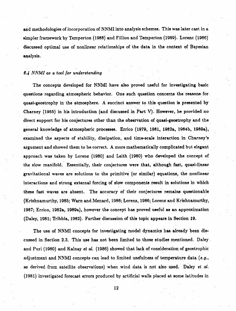
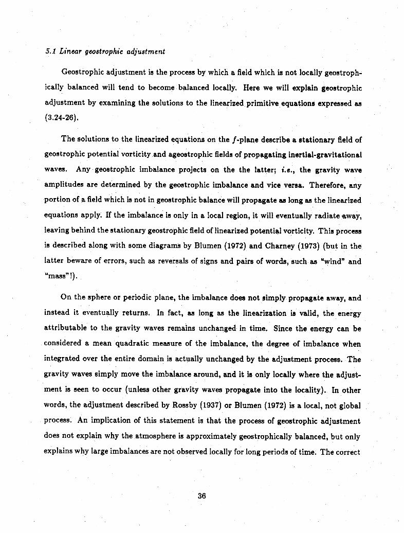
m= 1 n= 0 1=1 EG P = 33.0

2 110 10

PERIOD (hours)100

CLIMATE AND GLOBAL DYNAMICS DIVISION

NATIONAL CENTER FOR ATMOSPHERIC RESEARCHBOULDER. COLORADO

II

II

I

TABLE OF CONTENTS

List of Tables . . . . . . . . . . . . . . . . . . . . . . . .List of Figures . . . . . . . . . ... . . . . . . . . . .Preface . . . . . . . . . . . . . . . . . . . . . . . . . . .Acknowledgments ......................

Part I. INTRODUCTION

1.2.

Reasons for Initialization and Normal Mode AnalysisBrief History of Initialization . . . . . . . . . ..2.1 Initialization before development of NNMI . .2.2 Development of NNMI ............2.3 Problems and impacts of NNMI . . . . . . .2.4 NNMI as a tool for understanding . . . . . ..

.. . . . . ..aiv

.. . . . . . . Siv

....... vi

. l . . . ... vii

.. . . . . . . . .. .10 2

.. . . . . . . .12

Part II. DERIVATION OF NORMAL MODES

3. Presentation and Linearization of Model3.1 Nonlinear primitive equations .3.2 Linearization of equations . .

4. Solutions of Linearized Equations .4.1 Vertical structures ......4.2 Horizontal structures .....4.3 Field interactions . . . . . ..4.4 Sequence of transformations .

5. Dynamics of Linearized Model . .5.1 Linear geostrophic adjustment5.2 Linear initialization . . . . ..

. . . . . . . . . . . . . . . . . . 14. . . . . . . . . . . . . . . . .. . 16. . . . . . . . . . . . . . . . .. . 17

. .... ..... ..... ... 21. . . . . . . . . . . . . . . . .. . 22

. . . . . . . . . . . . . . . . . . . 26

................... 28

. . . . . . . . . . . . . . . . . . . 32. . . . . . . . . . . . . . . . .. . 35. . . . . . . . . . . . . . . . .. . 36

. . . . . . . . . . . . . . . . . . . 39

Part III. NONLINEAR CONSIDERATIONS

6. Nonlinear Normal-Mode Equations ............7. Scaling Arguments ...................8. Dynamics of Nonlinear Model ..............9. Machenhauer's Normal-Mode Balance Scheme .......

10. Physical Interpretation of Machenhauer's Balance Condition11. Determination of p ................ ...

. . . . . .. . 42

. . . . . .. . 45

. . . . . .. . 48.. . . . .. . 51

. . . . . .. . 52

. . . . . . . 55

Part IV. APPLICATION OF NNMI TO NUMERICAL MODELS

12. Vertical Modes for Vertically Discrete Models ...........

13. Explicit NNM I . . . . . . . . . . . . . . . . . . . . . . . . .14. Implicit NNMI . . . . . . . .. . . . . . . . . .. . . . . . .

15. Further Considerations .....................15.1 NNMI vs. no NNMI ....................15.2 Selection of modes to initialize ................15.3 Diabatic vs. adiabatic NNMI ................

15.4 Choice of starting iterates ...... ............

15.5 Consequences of incorrect mode determination .........

. . . .61

.. . a69

. .. . 73. . . .77

. .. . 77. . . 79

. . . .82... . 83

. ... 83

Part V. NNMI AND QUASI-GEOSTROPHIC THEORY

16. Scale Analysis in Terms of a Rossby Number . . . . .

17. Scale Analysis of Nonlinear, Diabatic Model Simulations .

17.1 Global model results ...............17.2 Mesoscale model results ..............

18. Description of Gravitational Modes as Oscillators . . . .

18.1 Demonstration of short-term behavior .......

18.2 Demonstration of long-term behavior . .. . .

19. Mode Forcing, Interaction, and the Slow Manifold . . ...

19.1 Stability of geostrophic waves and effects of dissipation

19.2 Slow Manifold . . ... .... . . . . .. .. .

Part VI. CONCLUSION

20. Summary . . . .. . .. . . . . . . . . . . . . .. ..

Appendix A: List of Mathematical Symbols .........

Appendix B: Determination of Nonlinear Interaction Coefficients

References . . . . . . . . . . . . . . . . . . . . . . . .

. . . . . . ... 86

. . . . . .... . 89

.. . . . . . .. 91

. . . . . . . . 95

. . . . . . .. . 99

. . . . . . .. . 99

. . . . . . . .103

. . . . . .. . 109

· . . . . . . . 110

.... . . . . 112

.. . . .. 117

.. . . .. 119

.. . . .. 122. . . . .. 126

LIST OF TABLES

Table 12.1. Values of a for data levels, standard atmospheric values of T at those levels,

and the set of equivalent depths H, determined for the standard CCM1. Note that t is a

a-level index for a and T, but refers to the ordering of the vertical modes in the case of

H . . . . . . . . . . . . . . . . . . . . . . . . . . . . . . . . . . . . . 63

Table 12.2. Values of a for data levels, standard atmospheric values of T at those levels,

and the set of equivalent depths H, determined for the standard 10-level MM4. Note that

e is a a-level index for a and T, but refers to the ordering of the vertical modes in the case

of H . . . .. . . . . . . . . . . . . . . . . . . . . . . . . . . . . . . . 64

Table 12.3. The matrix 0 which indicates the nonorthogonality of the vertical modes in

the MM4 for a standard atmosphere and 10 equally-spaced u-levels. The index t is listed

both vertcally and horizontally. An element of 0 with horizontal index i, and vertical

index t2 describes the projection of mode t4 on mode t2, and vice versa ..... 68

LIST OF FIGURES

Fig. 1.1 The time series of surface pressure as forecast by the CCM1 for a point nearEureka, California . . . . . . . . . .. . . . . . . . . . . 4

Fig. 12.1 The structures of the vertical modes of the standard 12-level CCM1 determinedfor a standard T profile ........................ 65

Fig. 12.2 The structures of the 10-level MM4 with equally-spaced a-levels for a standardT profile . . . . . . . . . . . . . . . . . . . . . . . . . . . . . . .66

Fig. 13.1 Time series of p,, T, a, g at a CCM1 grid point near Eureka, California as forecaststarting from a noninitialized and initialized analysis .. . . . . . 72

Fig. 14.1 Time series of p,,u,T, and w at a point near Detroit, Michigan for 24-hourforecasts begun from an initialized and noninitialized analysis ........ 76

Fig. 17.1 Spectra of normalized rms magnitudes of terms in the mode coefficient tendencyequation for selected sets of modes ................... 94

Fig. 17.2 Spectra of normalized magnitudes of terms in the 6-tendency equation at hour 48of a simulation for selected vertical modes .............. . 97

Fig. 17.3 Spectra of normalized magnitudes of normalized magnitudes of terms in the f - Vtendency equationat hour 48 of a simulation for selected vertical modes . . . . . . . . . . 98

iv

Fig. 18.1 Harmonic dials for selected modes in a noninitialized CCM forecast beginningfrom an ECMWF FGGE analysis ................... 101

Fig. 18.2 Response function R for the forcing of eastward propagation and westward prop-agation for a wave with resonance at a 33 hour period (eastward direction) and lineare-folding damping period of 5 days . . . .............. . 104

Fig. 18.3 Harmonic dials of four modes obtained near the end of a long climatesimulation . .. . .. . .. . . . . . .. . . . . . . . . . . . ... 106

Fig. 18.4 Power spectra of modes corresponding to Fig. 18.3 .......... 107

Fig. 19.1 A schematic representation of the slow manifold in a simple two-componentm odel . . . . . . . . . . .. . . . . . . . . . . . . . . . . . . . 115

v

PREFACE

Just prior to being appointed an Adjunct Associate Professor in the Department of

Meteorology at the University of Utah, I was asked to present a series of lectures on the

subject of normal mode initialization. These were delivered in May 1987 during a two-week

period. Approximately 20 students and faculty attended the 6 one-hour lectures. Morecondensed versions of these lectures have been presented at other institutions, and stillothers have asked for copies of my notes. This technical note is derived from these notes

and from several of my papers on the subject of normal mode initialization, but its form

is more readable than the notes and more succinct than the collection of papers.

The above situation provided the possibility of preparing this technical note, but the

motivation was not simply to publish a set of notes. During my fifteen years of work on thesubject I have come to realize that normal mode initialization is not just some "trick" usedto remove forecast noise. Rather, the subject is basic to dynamic meteorology. In fact, most

principles, limitations, and extensions of quasi-geostrophic theory can be derived from this

theory in a straightforward and elegant manner. Also, since it uses a linear theory as a basisto investigate nonlinear behavior, it is simple to comprehend but not restricted to linear or

quasi-linear contexts. For many studies, the normal modes themselves or their associated

initialization theory in general provide a valuable tool for investigating and understanding

complex atmospheric behavior. For these reasons, it is my firm opinion that the theory and

principles of normal mode initialization should be part of the core curriculum of graduate-

level dynamic meteorology. Although not as detailed as a textbook, this technical note isintended as an aid in such a curriculum.

Ronald M. Errico

NCAR

September 1989

vi

ACKNOWLEDGMENTS

Although I was not well aware of all the connections at the time, the subject of thistechnical note was also the subject of my Ph. D. thesis. The question investigated in thatthesis was "Why is the atmosphere nearly quasi-geostrophic", for which I thank my thesisadvisor E. N. Lorenz for posing to me. Since the thesis was completed in 1979, it has beendifficult for me to stray far from the topic because of its many applications and intriguingaspects.

While at NCAR I have benefited greatly from the presence of many colleagues whohave contributed greatly to the theory and application of normal mode initialization.Among them were (at various times) the members of what is now called the GlobalDynamics Section of the Climate and Global Dynamics Division at NCAR. These wereR. Daley, D. Williamson, A. Kasahara, J. Tribbia, and C. Leith.

The PSU/NCAR mesoscale model was provided by courtesy of R. Anthes and colleagues.The CCM was provided by D. Williamson and colleagues. The Navy models and analysis

were provided by E. Barker, R. Gelaro, and colleagues.

The lectures at the University of Utah were at the invitation of J. Geisler, and J. andJ. Paegle. The more abbreviated lectures at the Naval Postgraduate School were at theinvitation of R. T. Williams. F. Carr at the University of Oklahoma and R. Daley alsoencouraged me to distribute a readable version of my notes.

R. Bailey provided invaluable assistance in preparing the manuscript. G. Bates pro-vided assistance in preparing final versions of the figures. Both he and B. Eaton also aidedme at various times in preparing normal mode software for use at NCAR.

vii

Part I. INTRODUCTION

According to its title, this report is intended to serve as a comprehensive summary

of the theory and application of nonlinear normal mode initialization (NNMI). NNMI

was developed in the late 1970s for initialization of models used for numerical weather

prediction (NWP). It was originally developed and described in terms of normal modes of

linearized versions of the models; i.e., in terms of the independent solutions to particular

eigenvalue problems. In contrast to earlier initialization schemes using normal modes,

terms previously treated as nonlinear, and therefore neglected in the eigenvalue problems,

were reconsidered by NNMI. Although many questions and details regarding its application

remained unanswered, NNMI proved quite successful as an initialization procedure, and

during the 1980s it or its derivatives became the standard initialization technique.

In the future, as observation, analysis, and forecast systems improve, it is not certain

that NNMI will remain an appropriate initialization procedure. However NNMI should

not be regarded as only an engineering tool which may or may not be useful in some NWP

system. Rather, the theory and framework of NNMI is fundamental to the dynamics

of forecast models and the relationships between various types of atmospheric data. In

fact, the theory can be considered as more fundamental than quasi-geostrophic theory,

since the latter may be considered as a low-order approximation to NNMI theory, and

since NNMI theory reveals the processes which maintain quasi-geostrophy in both models

and the atmosphere. Also, since it is based on linear and quasi-linear concepts, NNMI is

relatively easy to interpret, and its framework provides a useful tool for the analysis of

model responses to both data input and internal forcing.

Almost all global atmospheric data analyses and many regional data analyses are

produced by data assimilation systems. These systems use a numerical forecast model to

interpolate or extrapolate information into data-void regions through production of short-

term forecasts. Most systems also use some form of NNMI. For this reason, the possible

1

effects of NNMI should be considered when interpreting these analyses, even in a non-NWP

context. In some cases, the effects of NNMI on even large-scale time-mean fields may be

quite profound (c.g., see Rosen and Salstein, 1985). The relevance of understanding the

principles of NNMI, therefore, currently extends well beyond the subject of NWP.

In this report, the word "initialization" is used exclusively in the restricted sense of an

adjusting or constraining of data for use as initial conditions in model forecasts, especially

for NWP. The process of producing data on some regular grid or in terms of coefficients

of structure functions (e.g., spherical harmonics) using irregularly-spaced observations is

called "analysis. Such analysis is necessary to begin a numerical forecast, since models

necessarily represent data in some structured way. (However, the word "analysis" will not

be used exclusively in this sense.) An analysis must always be performed prior to producing

a forecast, but an initialization is not strictly necessary. Discussion of the analysis problem

is not an intention of this report, except as it relates to some aspects of the initialization

problem. For discussion of the analysis problem see, e.g., Bengtsson et al. (1981).

In Part I of this report, the purpose of initialization is discussed, followed by a brief his-

tory of solutions to the problem of initialization. Attention is focused on NNMI rather than

on earlier schemes. In subsequent parts: (Part II) a simple model is used to introduce and

describe normal modes and the phenomenon of linear geostrophic adjustment; (Part III)

nonlinear aspects are reintroduced and NNMI described; (Part IV) the applications of

NNMI to global and regional models are presented; (Part V) and the relationship of NNMI

to quasi-geostrophic theory is discussed. A summary stressing the use of NNMI is presented

in Part VI.

1. Reasons for Initialization and Normal Mode Analysis

The motivation for using NNMI is discussed in this section. Since this section is

intended as an introduction only, most literature citations will be omitted. Instead, other

sections of this report will be referenced, and details and citations will be found in them.

2

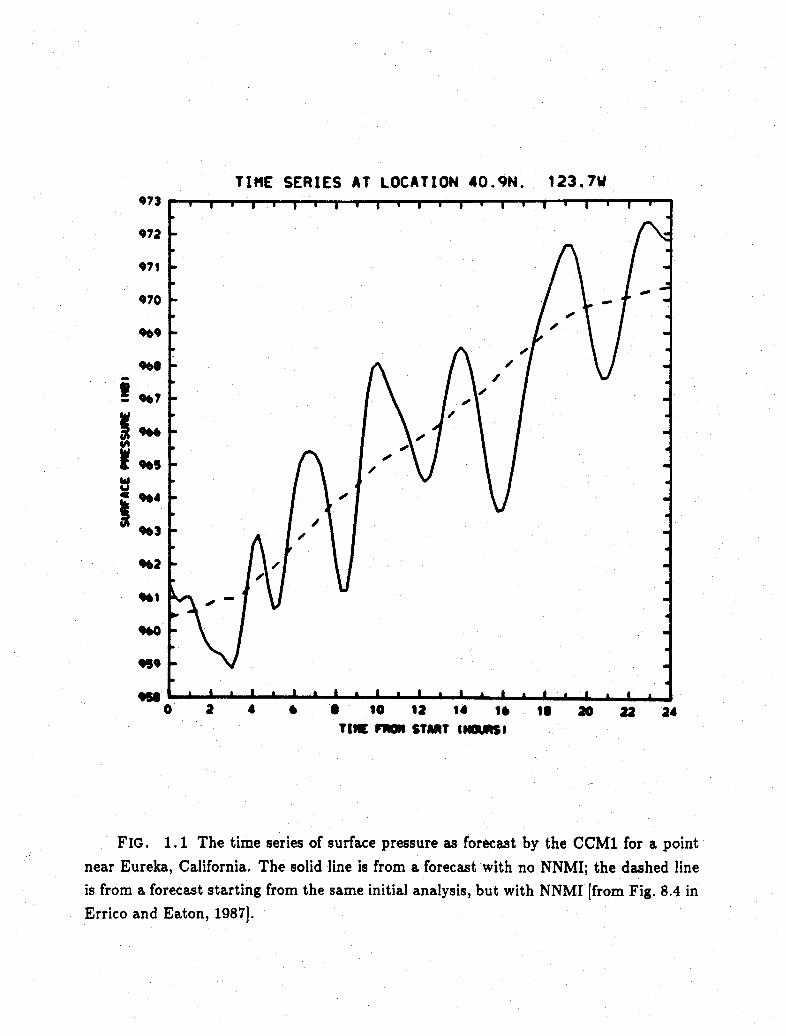
An example of a time series of surface pressure near Eureka, California as forecast by

an NWP model is presented in Fig. 1.1. The model is version 1 of the NCAR Community

Climate Model (CCM1), initialized with an analysis produced for OZ 16 January 1979.

The forecast is described more completely in Section 13.

The time series produced when no initialization has been performed is indicated by

the solid line in Fig. 1.1. Note that the behavior of the surface pressure has two primary

characteristics: there is a gradual increase of approximately 10 mb during 24 hours, and

there is a superimposed, rapid oscillation with changes as large as 5 mb in two hours.

Similar characteristics of the surface pressure forecast are observed at all other locations

in the model during this forecast period. Also, most other dynamic fields are similarly

characterized as having both slow and fast components, but to greater or lesser degrees

(for some examples, see Section 13).

A barograph of the verifying observed surface pressure for the same time and place

as Fig. 1.1 has not been prepared. Generally however, fast-changing components of the

surface pressure with amplitudes as large as in Fig. 1.1 are rarely observed anywhere,

whereas in the CCM1, they are observed during the first day (or longer) for nearly all

forecasts, everywhere. Clearly, the forecast of these components is unrealistic. There are

errors somewhere in the CCM1 or in the analysis used to start the forecast.

The existence of unrealistically large, high-frequency components in the forecast may

or may not have a significant impact on the use made of the forecast (Section 15). Their

presence may simply render interpretation of forecast synoptic maps more difficult, or,

much worse, they may trigger unrealistic convection and thereby destroy the utility of

a forecast. One significant problem has been the degrading of analyses which use noisy,

short term model forecasts as a source of data (background information) in addition to

observations. Clearly, even if this degradation has little impact on a specific application,

it is worthwhile to investigate, understand, and correct the problem in order to properly

3

TIME SERIES AT LOCATION 40.9N.973

972

971

970

90*

'.9

9.5

,,1

'.,

950«5«

VA0 2 4 * * 10 12 14 16 is 20 22 24

TINE F STMT IndOSI

FIG. 1.1 The time series of surface pressure as forecast by the CCM1 for a point

near Eureka, California. The solid line is from a forecast with no NNMI; the dashed line

is from a forecast starting from the same initial analysis, but with NNMI [from Fig. 8.4 in

Errico and Eaton, 1987].

123. 7WAh 40 du -- -

I

assess its impact and to prepare for future systems where smaller errors may increase the

relative significance of this kind of initial noise.

The amplitudes of the high-frequency components (often called "noise") in forecasts

depend on many characteristics of the model and its initial analysis. For this reason, the

amplitude shown in Fig. 1.1, although typical of CCM1 forecasts, should not be considered

typical of other models. However, unless the noise problem is specifically rectified, all

primitive-equation forecasts have such noise to some noticeable degree. The amplitude of

noise in the surface pressure field generally decreases with time, although the same may

not be true for some other fields. In global models, the rate at which noise decreases

will depend on characteristics of the model's physical and numerical dissipation (Errico

and Williamson, 1988), and in limited-area models it also will depend on the domain

size and the formulation of lateral boundary conditions (Warner et al. 1984; Errico and

Baumhefner, 1987). Some of these points are discussed in Sections 17 and 19.

Actually, the source of this noise has been known for a long time (Section 2). Most

NWP models admit inertial-gravitational waves as components of their general solutions.

Analysis inaccuracies will usually result in the presence of such waves in subsequent

forecasts, unless some adjustments of the data are made. The process of adjusting the

data for this purpose is called initialization. It is related to the process of geostrophic

adjustment, as discussed in Sections 5 and 8. Many different but related initialization

schemes have been developed since the advent of NWP, but the most successful one has

been NNMI.

Before proceeding to discuss initialization, it is pertinent to mention that other solu-

tions to this unrealistic wave problem have been used. Quasi-geostrophic models do not

admit such waves in their forecasts, although they also miss other effects due to their

filtering of even slow inertial-gravitational components. Other filters, such as selective

diffusion have been applied to NWP models, for which a difficulty is to restrict their

effects to only the unrealistic components. Filters have also been applied successfully

5

to forecasts themselves; i.e., after forecasts have been produced by the models (e.g.,

Williamson and Temperton, 1981; Kuo and Anthes, 1984). Of course, if any unrealistic

waves have impacted the slower components of the forecast, their impact is not removed

by such subsequent filtering.

The method of NNMI is described primarily in Parts II-IV and its application specif-

ically to the forecast in Fig. 1.1 is described in Section 13. However, for the purpose

of putting what follows in perspective, the results of applying NNMI to that forecast

are also presented Fig. 1.1 as the dashed line. Note that the initial surface pressure at

this location has been reduced by approximately 1 mb. Thereafter, the time series from

the initialized forecast is almost precisely that which would be created by subjectively

smoothing the noninitialized time series: the slow pressure rise with time appears to be

reproduced almost precisely as seen in the noninitialized forecast, but any superimposed

high-frequency oscillations are almost undetectable. It should be emphasized that the

differences between the two time series have been produced by starting the forecasts from

only slightly different initial conditions and not by any subsequent alteration of the model.

The NNMI technique explicitly considers the structures and behaviors of inertial-

gravitational waves. Therein lies one cause of its successful application. However, this

consideration also renders aspects of the NNMI technique useful for many analyses of model

behavior, especially when slow and fast model components are to be formally distinguished.

For this reason, the theory and application of NNMI should remain useful even beyond a

time, if ever, when initialition is no longer explicitly useful for NWP.

2. Brief History of Initialization

The intention of this section is to provide a brief overview of initialization in general

and NNMI in particular, as well as examples of the use of normal modes as a tool for

understanding model results. A good review of initialization prior to NNMI may be found

in Bengtsson (1975) while NNMI has been reviewed by Daley (1981a). The use of the

6

NNMI framework as an analysis or theoretical tool has not be reviewed in any detail. In

this section, many contributors to the development of initialization and NNMI will likely

be neglected. Further citations may be found throughout this report as well as in the lists

of references in the cited literature.

2.1 Initialization before development of NNMI

The need for initialization was first observed in Richardson's (1922) famous experiment

where he attempted to use the primitive equations for producing a numerical forecast

of weather in Europe. He lacked sufficient data (there was no rawindsonde network at

that time), with the result that forces determined from his initial fields were so in error

that huge dynamic tendencies were obtained. These tendencies were so unrealistic that

Richardson abandoned his attempt. It was not until the advent of the modern computer,

the development of quasi-geostrophic theory by Charney (1948) and others, and a global

observation network, that numerical forecasting in general, and the use of the primitive

equations in particular, were re-attempted. For discussion of some aspects of this history,

see e.g., Platzman (1987).

The presence of Richardson's large initial tendencies is related to the phenomena of

geostrophic adjustment (Section 5). The principles of linear geostrophic adjustment date

back at least to Rossby (1937, 1938) who showed how to derive a final geostrophically

balanced state from initial conditions in a barotropic atmosphere (see also the review by

Blumen, 1972). Hinkelmann (1951) and Charney (1955) related the presence of large

initial tendencies in numerical forecasts to this adjustment process: Essentially, a portion

of the errors in the initial conditions are interpreted by the model as due to the presence

of (unrealistic) inertial-gravitational waves which subsequently propagate throughout the

forecast and appear as meteorological (gravitational) "noise". Larger analysis errors tend

to yield greater noise. Charney (1948) earlier had shown how to derive a set of equations

which excluded such noise (the quasi-geostrophic equations), however it was clear that some

7

important meteorological activity was thereby modelled poorly (e.g., fronts and tropical

circulations). Other exclusionary equations were also developed (e.g., the semi-geostrophic

equations; Eliassen, 1948; see also Hoskins, 1975), but some appropriate initialization

scheme for using the primitive equations without unrealistic noise remained desireable.

Charney (1955) showed that gravitational noise could be reduced within forecasts

which used the primitive equations by constraining the initial condition to satisfy a non-

linear balance equation. Satisfaction of a linear geostrophic relationship also may reduce

noise, but the nonlinear balance equation produced significantly better results. Charney's

balance equation concerned only the rotational part of the wind, however Phillips (1960)

showed that consistency required that the divergent part of the wind should also be

constrained to satisfy a kind of balance equation, specifically a form of the quasi-geostrophic

omega-equation. These results of Charney and Phillips are discussed in terms of NNMI in

Section 10.

Miyakoda and Moyer (1968) and Nitta and Hovermale (1969) developed methods

which effectively filtered gravitational noise from primitive-equation forecasts by using the

model dynamics and numerical scheme. Their methods have been denoted as dynamic

initialization schemes, since they require time integration of the equations in order to

specify even the initial condition. These methods should be contrasted with the previous

static schemes which only applied balance condition constraints at the initial time. The

dynamic schemes were sufficiently successful so that primitive equation models became

the standard for numerical weather prediction. However, because the filters used by those

methods were not so selective as to affect only components responsible for the noise,

these early schemes had drawbacks, notably including a general weakening of the entire

circulation. Recently these dynamic schemes have been recast in the framework of NNMI

(Sugi, 1986), with many of the earlier drawbacks diminished.

8

2.2 Development of NNMI

In many contexts, waves are quasi-linear phenomena, and it had been known for a

long time that one class of solutions to the linearized primitive equations described inertial-

gravitational waves. Dickinson and Williamson (1972) used that knowledge to define an

initialization scheme which attempted to filter high-frequency waves from model initial

conditions. This method has since been called linear normal mode initialization. It was

not very successful. The reason for this result is discussed in Section 8, and primarily

regards the neglect of consideration of nonlinear effects on the gravitational modes.

Nonlinear balance equations were first described in terms of normal modes by Machen-

hauer (1977) and Baer (1977). Machenhauer considered the prognostic equations for

amplitudes of gravitational modes, and showed that with or without initialization, the

adiabatic nonlinear forcing term has a strong, slowly varying component. This yields a

correspondingly slow response, which approximately satisfies a nonlinear balance equation

expressed in terms of the normal mode amplitudes and their forcings. He proceeded

to show how solutions to this new balance condition could be determined and applied

to the initialization problem. Baer applied a Rossby number scaling to the primitive

equations schematically expressed in terms of the normal modes and explicitly considered

the presence of multiple time scales. He showed that asymptotically slow solutions were

possible, and that these solutions were characterized by a nonlinear balance condition

expressed in terms of the normal modes. This work was later extended by Baer and

Tribbia (1977) to the practical application of this result to the initialization problem.

The methods of Machenhauer, Baer, and those who built on their work, are collectively

called nonlinear normal mode initialization schemes. They were applied to some global

forecasting systems by Andersen (1977), Daley (1979), and Williamson and Temperton

(1981), among others, and also to regional models by Briere (1982), Du Vachat (1986),

and others. Machenhauer's scheme was used predominately, although the scheme of Baer

and Tribbia provided a more suitable theoretical framework for many problems.

9

Soon after NNMI was presented by Machenhauer and by Baer, it became apparent that

the NNMI balance equations were related to the nonlinear balance equations of Charney

(1955) and Phillips (1960), but it was unclear what that precise relationship was. Leith

(1980) used the context of an f-plane model to show their specific relationship. Bourke

and McGregor (1983) subsequently developed an NNMI scheme which only explicitly

considered the vertical structures of the modes, resulting in a simpler application of NNMI

to regional models for which horizontal mode structures were more difficult to determine.

Temperton (1988) has presented an elegant mathematical demonstration of the equivalence

of the Bourke and McGregor method with that of Machenhauer applied to the same model.

He has termed schemes which use only the vertical structures "implicit" NNMI schemes,

as contrasted with "explicit" schemes which require determination of the modes' complete

three-dimensional structures.

Many other initialization methods have been developed since the advent of NNMI.

Some are described throughout this section and this report where applicable. For all these

schemes, NNMI provides a benchmark with which to compare results and a theoretical

framework with which to explain methodologies and reasons for success.

2.S Problems and impacts of NNMI

There are several works which discuss various aspects of the results of NNMI, regarding

its effects on both analysis systems and forecasts. Daley (1979) showed that precipitation

forecasts were not greatly improved in his model by the incorporation of NNMI, which

was a reminder that NNMI could only definitely improve those components of the forecast

which it was specifically designed to affect (i.e., gravitational noise). Bengtsson (1981)

revealed that some applications of adiabatic NNMI tended to weaken tropical circulations.

Wergen (1983) introduced a diabatic NNMI scheme to alleviate that tendency. Essentially

both he and Bengtsson reasoned that since tropical circulations are diabatically driven,

adiabatic NNMI would fail to produce realistic tropical circulations. Errico (1984b, 1989a,

1989b), Errico and Rasch (1988), and Errico et al. (1988) suggested that the poor results of

10

applying adiabatic NNMI in the tropics were not only due to neglect of diabatic processes

there, but equally to the inappropriateness of the NNMI balance condition itself within

the tropics (at some scales; see Part V).

Another problem noted in the applications of NNMI was the lack of general conver-

gence of Machenhauer's (1977) scheme for obtaining iterative solutions (e.g., Williamson

and Temperton, 1981). The problem was discussed using a one-dimensional model by

Ballish (1981) and in more general contexts by Errico (1983) and Rasch (1985a). Rasch

(1985b) and Lynch (1985) introduced alternative schemes with better properties for

obtaining the desired NNMI fields. Kitade (1983) introduced an under-relaxed version

of Machenhauer's scheme, but its improved convergence was limited for reasons discussed

by Errico (1983). Thaning (1983) showed that in some cases, multiple or inappropriate

solutions may exist, although his context was for a simple model and high Rossby number.

The question of which horizontal and vertical scales should be modified by NNMI

also has received much, although insufficient, attention. For most NNMI schemes, the set

of initialized modes or scales is restricted in practice by a lack of general convergence of

their iterative solutions as previously discussed. Puri and Bourke (1982) and Puri (1983,

1985, 1987) examined relationships between convection and initialization. Errico (1984b,

1989b, 1989c), Errico and Rasch (1988), and Errico et al. (1988) used model simulations

in an attempt to deduce which scales are balanced in the atmosphere. Carr et al. (1989)

compared forecasts produced with different scales initialized, and showed that a more

restricted set of modes performed better with their particular NNMI scheme and forecast

and analysis system.

Initialization is most important in the context of data assimilation, as reviewed by

Bengtsson (1975, 1981) and discussed in Section 15. Static balance constraints were

considered by Sasaki (1956) in the context of variational analysis methods. Flattery

(1967) considered analysis of the rotational normal modes. Daley (1980), Williamson et al.

(1981), Tribbia (1982), and Williamson and Daley (1983) discussed the appropriateness

11

and methodologies of incorporation of NNMI into analysis schemes. This was later cast in a

simpler framework by Temperton (1988) and Fillion and Temperton (1989). Lorenc (1986)

discussed optimal use of nonlinear relationships of the data in the context of Bayesian

analysis.

£.4 NNMI as a tool for understanding

The concepts developed for NNMI have also proved useful for investigating basic

questions regarding atmospheric behavior. One such question concerns the reasons for

quasi-geostrophy in the atmosphere. A succinct answer to this question is presented by

Charney (1955) in his introduction (and discussed in Part V). However, he provided no

direct support for his conjectures other than the observation of quasi-geostrophy and the

general knowledge of atmospheric processes. Errico (1979, 1981, 1982a, 1984b, 1989a),

examined the aspects of stability, dissipation, and time-scale interaction in Charney's

argument and showed them to be correct. A more mathematically complicated but elegant

approach was taken by Lorenz (1980) and Leith (1980) who developed the concept of

the slow manifold. Essentially, their conjectures were that, although fast, quasi-linear

gravitational waves are solutions to the primitive (or similar) equations, the nonlinear

interactions and strong external forcing of slow components result in solutions in which

these fast waves are absent. The accuracy of their conjectures remains questionable

(Krishnamurthy, 1985; Warn and Menard, 1986; Lorenz, 1986; Lorenz and Krishnamurthy,

1987; Errico, 1982a, 1989a), however the concept has proved useful as an approximation

(Daley, 1981; Tribbia, 1982). Further discussion of this topic appears in Section 19.

The use of NNMI concepts for investigating model dynamics has already been dis-

cussed in Section 2.3. This use has not been limited to those studies mentioned. Daley

and Puri (1980) and Kalnay et at. (1986) showed that lack of consideration of geostrophic

adjustment and NNMI concepts can lead to limited usefulness of temperature data (c.g.,

as derived from satellite observations) when wind data is not also used. Daley et al.

(1981) investigated forecast errors produced by artificial walls placed at some latitudes in

12

models. The importance of NNMI for understanding predictability studies was emphasized

by Errico and Baumhefner (1987).

Model normal modes have also been used for climate studies. Paegle et al. (1986)

used them to investigate interactions between the tropics and extratropics in studies of

the atmospheric response to sea surface temperature anomalies. Gelaro (1989) used them

in a different manner for a similar investigation. Kasahara and Puri (1981) and Tanaka

and Kung (1988) have examined normal mode coefficients determined from atmospheric

analyses. Branstator (1989) has demonstrated that consideration of normal modes of

complicated basic states can yield substantial insight into low frequency behavior andseasonal climate. These newer works suggest that analyses using normal modes will

continue to be useful for understanding of atmospheric behavior on many time scales.

13

Part II. DERIVATION OF NORMAL MODES

In this part, the normal mode equations are presented. They are derived for a

model defined on a plane with periodic boundary conditions, although the differences and

similarities with modes on a sphere are discussed at the end of Section 4. The application

to a periodic domain on a plane greatly simplifies the transformation between normal-mode

and physical-space descriptions, and therefore is very appropriate for pedagogic purposes

(Leith, 1980).

The complete adiabatic model is presented in Section 3 along with an appropriately

linearized version. The solutions of the linearized version are then determined from an

eigenvalue problem in Section 4. Their properties are discussed in Section 5 in the contexts

of the process of linear geostrophic adjustment and the technique of linear initialization.

The usual notation is used where no conflicts occur, and any unusual or ambiguous

notation is defined when introduced. For reference, a variable list appears in Appendix A.

3. Presentation and Linearization of Model

The model uses the primitive equations. These equations permit the propagation

of gravity waves, but not sound waves. Equations which filter gravity waves, such as the

quasi-geostrophic equations, would not yield the types of modes in which we are interested.

The horizontal coordinates are a Cartesian z (increasing eastward) and y (increasing

northward) with corresponding velocity components u and v. The domain is specified as

periodic in both directions, with some fundamental wavelength LF; i.e., for any field a,

14

a(x ,y) = a(x, y + LF)(3.1)

=a(x + LF, y).

This condition is not strictly necessary, but allows the use of simple trigonometric functions

for the description of the normal modes. More general boundary conditions for limited-area

models are discussed in Briere (1982). However, (3.1) corresponds closely to the condition

on the sphere (which is also a periodic domain). Condition 3.1 also places restrictions on

the z, y dependence of the Coriolis parameter f if solutions are to remain periodic for all

time. However, since many types of conditions and approximations are possible, none is

explicitly stated here, since such details are unnecessary for all the derivations to be made

below. Most simply, we may just consider that f = fo everywhere, but at the end of

Section 4 we will describe important effects due to variable f on the sphere.

The vertical coordinate is sigma, defined as

a = -, (3.2)P.

where p is the pressure at some height and p, is the pressure at the surface. The top and

bottom of the model are therefore a = 0 and o = 1, respectively. The use of other vertical

coordinates may change details of the form of the equations, but all qualitative comments

regarding the form of the solutions must apply equally well to other coordinates; i.e., the

properties of the solutions are not altered by a coordinate change, although the exact

expression of those properties may be altered. The direction perpendicular to a surface of

constant a will be simply called the vertical, and that surface will be called horizontal.

Terms which describe the diabatic processes are simply denoted by D with subscripts

to denote the equations to which they are applied. Different diabatic processes will not be

distinguished until Part V.

15

S.1 Nonlinear primitive equations

The nonlinear equations are

auatavat

aTat

a In(p,/p)at

au au .9u auxV + V + o y +fv-- [O + RT ln(p./p)] + Dv

UT + v j- +a 6-fu- [ + RTln(p./p)I+Dv

aT aT aTu-+ V-+ V a-+ T-+ +DTx ady aa p

- I 6daJo

(3.3)

(3.4)

(3.5)

(3.6)

(3.7)

(3.8)

(3.9)

(3.10)

(3.11)

The first four equations are prognostic and the remaining ones diagnostic. These equations

are derived from the conservation of momentum (3.3-4), the first law of thermodynam-

ics (3.5), the conservation of mass (3.6), and the hydrostatic relationship (3.7). The

variable a may be interpreted as a counterpart to the vertical component of velocity in a-

coordinates; 6 is the velocity divergence on a a-surface, hereafter simply called divergence;

and ¢ is the vertical component of relative vorticity, hereafter simply called vorticity. At

this point, the use of 6 and $ may simply be considered as abbreviations for the sums and

differences of the indicated differentials.

16

, _|r RT0 = 6 - - daI ay

p ao a

v = a E da - 6 da

, u . v

( x 9y

9.2 Linearization of equations

The propagation of many waves in the model and atmosphere may be considered as

a quasi-linear phenomenon, as demonstrated in Sections 5 and 18. For this reason, since

our particular interest is in gravity waves, it is appropriate to consider a linearized form

of the model equations. To do this we define an appropriate basic state (denoted by a

bar over the variables) and a perturbation from that state, and ignore any terms which

involve products of two or more perturbation variables. Further, we select the basic state

such that either it itself is a stationary (i.e., time-independent) solution to the nonlinear

equations, or assume that some unspecified external forcing renders it stationary.

The selection of the basic state must be done carefully. The two primary considerations

are that the resulting linearized equations are solvable by some means (or that at least

we learn something from them) and that those equations describe significant aspects of

the dynamics. The first consideration motivates us to make the basic state as simple

as possible, and the second motivates us to make it as complex as possible to minimize

the labeling of dynamic terms as nonlinear with their subsequent neglect when only the

linearized terms are retained. Since these are conflicting considerations, selection must

depend on the exact purpose of the linearization.

For the purpose of NNMI, the linearization primarily is used to separate the dynamic

fields into portions which describe either gravity waves or quasi-geostrophic fields. Different

basic states will likely yield different separations, so that even if the NNMI scheme directly

affects only gravity waves, the actual effect on the dynamic fields will differ as the basic

state is varied. This will be further discussed in Section 15.5. In NNMI, the terms neglected

in the linearization are not just discarded, but they are instead reconsidered (Part III), so

that the linearization acts to distinguish terms rather than filter effects.

The most typical basic state chosen for NNMI is a resting, horizontally uniform,

convectively stable atmosphere. This may be denoted by

17

u=0

v-0

= T((a) (3.12)

In P. = constant

= ¢(To,)

e=0o

The last is a condition that there are no mountains. The resulting basic state is a stationary

solution to the adiabatic, primitive nonlinear equations. Also, this basic state yields

separable linear equations which are especially easy to solve, as discussed below. The

linearization is about a Inp. rather than about p* because p, explicitly appears in the

adiabatic equations for this model only in the form of In p,, and this linearization therefore

acts to retain more of the explicit pressure effects on the dynamics without making the

equations more difficult to solve. The horizontal means of T(a) and In p, determined from

some analysis may be used to define the basic state, or a standard atmosphere may be

used. Furthermore, we can define p = exp (in p,).

The linearization will be about a constant value of f, denoted fo, since this greatly

simplifies the solutions to the linear equations. On the sphere this simplification is not

made (Appendix B). On the plane, this restriction does affect the linear solutions as will

be noted, but the nonlinear initialized solutions are less affected. Any term involving

a deviation of f from fo will be considered a nonlinear term, to be neglected by the

linearization, but reconsidered by the NNMI.

The resulting adiabatic linear equations are

t = fov - y [' + RTln(p,/p)] (3.13)

= -f^u^- [(1 +RTIn(p./p)] (3.14)

18

AT' Tt = -a-°, +cKT- (3.15)at Qa P

Oln(p/p) = j|6 do (3.16)

l e- oRT' (3.17)a

w = -- l 6 do (3.18)

po o6= a j do- 6 do (3.19)

a = oz + _ (3.20)Ox Oy

- ^ =v - U a(3.21)

where superscript primes on T and b indicate departures from the mean state, but no

primes are indicated for u, and v, w, 67, 6, or f since their basic state is 0. These should

be compared with (3.3-11), respectively. Note that the presence of mountains (4,) is

considered as a perturbation effect.

The quantity whose gradient describes the linearized pressure gradient force in a-

coordinates is the pseudo-geopotential p defined as

cp = X' + RTln(p,/p) (3.22)

Its time tendency may be determined by combining all the diagnostic equations and

thermodynamic equations to yield the integral-differential equation

9Po f OT \ T

aOt R 1 [(2 a- a) l6& "] d" da' -RT(1) 6 da' (3.23)

The operations on 6 which comprise the right-hand side of (3.23) are denoted as (the

operator) r, so that the four prognostic linearized equations may be written simply as

at9 = ' -fo- i(3.24)at= fo xz

19

aOv _- ou-(3.25)at =- - ay

ai = -r8() (3.26)

ain(p./) = _f (3.27)

It is also useful to define the differential operator which corresponds to r, written as

r-l, which satisfies

rr--(a) = r 1- r(a) = a, (3.28)

where a is any dynamic field. The operator is

r-'(a) -R - a r aa, (3.29)

with boundary conditions

aa { _0a at a=1 (3.30)

whereKT 89T

r - (3.31)a a

is a mean static stability parameter. If a is the field 6 then the boundary conditions are

equivalent to = 0 at a = 1 and 0.

Equations 3.24-27 are the linearized adiabatic primitive equations. It is easy to show

that they conserve the sum of a quadratic form of the kinetic and available potential

energies per unit mass, defined as

E JO Jj JO +. .+u2+v2] dxdy da (3.32)

As successive transformations of the linearized equations are considered in Section 4, the

corresponding expressions for E in terms of the transformed fields will be presented in

order to complete the description of each transformation.

20

4. Solutions of Linearized Equations

Equations 3.24-26 comprise an eigenvalue problem. Schematically, we may write

[u(x,y,at) [u(x, y, o,t)d | v(xy,ot) = C v(x,y, a,t) I, (4.1)

(t x y(,y,o,t) ("( ,y, , t)]

where ZC is a linear operator which includes horizontal derivatives and vertical integrals.

If expressed in finite difference form, ZC could be written as a matrix operator. However,

because of the simple basic state chosen, it is possible to solve (4.1) analytically. We note

that it is not necessary to also consider the linearized prognostic equation for In p./p (3.27)

since it is already implicitly considered in (3.26). However, if the linearized behavior of p.

is to be examined, then (3.27) must be considered, as we will do in Section 11.

The form of the operator £ and the simplicity of the boundary conditions (3.1) allows

us to obtain separable solutions to (4.1); i.e., we can separate the operations of £ by

considering

£(x,y,a) = AC £C £y £c(H,m,n,A) (4.2)

where the subscripts indicate the coordinates to which the operators apply and the values

H,m, n, A are respective eigenvalues of the operators £, C, ,^Cy, £C. In other words,

each of £<, a,C Cy describe an independent eigenvalue problem, which depends on linear

operations in one coordinate direction only. The operator ce is that which describes the

coupling of the u, v, and p fields. Each of these sub-problems is easier to solve individually

than when considering £ as a whole. The separability of the operator implies a separability

of its solutions as, e.g.,

u(x,y,a,t) = ZH(a) sm(x) s. (y) a(H,m,n)e t, (4.3)

where each function on the right-hand side is described separately in the following

subsections.

21

4.1 Vertical structures

The linear operator 4 is equivalent to the operator r since it is the only operator in

a. The eigenvalue problem for r is

r zt = gHe Zt (4.4)

The ze are only functions of a and are called vertical structure functions or vertical modes

since all the a-dependence of the solutions is described by these functions. Corresponding

to each eigenvector ze is the eigenvalue gHe where g is the acceleration of gravity. Each

Ht is called an equivalent depth for reasons discussed at the end of this section and in

Section 5. For the vertically-continuous equations, there are an infinite number of vertical

modes (! = 1,... ,0o), but for a discrete model where the fields u, v,o are defined-on L

a-surfaces, there are only L vertical modes.

Equation 4.4 is an integral equation. If instead the corresponding differential equation

is considered,

r-lzt() = ze() (4.5)

with the boundary conditions (3.30), the resulting eigenvalue problem for the vertical

modes is seen to be a Sturm-Liouville problem. Solutions to this type of problem have

many relevant properties: in particular, if the basic-state static stability (r) is positive

valued for all a, then

1. all HI are positive real values;

2. there is a maximum value of Ht, called the equivalent depth of the external

mode;

3. the He may be ordered as a series of descending values, with each successive

corresponding vertical mode having one more zero crossing than the previous

mode (therefore e - 1 may be interpreted as the number of sign changes zt has

between a = 0 and 1.

22

4. vertical modes for different e are orthogonal to one another; i.e.,

k,t = I Zk(a) Zt(a) da, (4.6)o

where P is the Kronecker delta

1 if k =t;Dk,= {o ifk e. (4.7)

Condition 4 has also used the property of all linear eigenvalue problems that a constant

times any eigenvector is also an eigenvector, so that all the eigenvectors may be normalized

to yield the value 1 for k = e in (4.6). A mathematically detailed summary of the vertical

mode problem in differential form, especially regarding its boundary conditions, appears

in Cohn and Dee (1989).

For comparison with the vertical eigenvalue problem in vertically-discrete models, it is

worthwhile to note that, for an inner product of the form (4.6), an adjoint of a differential

operator r-1 is a differential operator r-1T which satisfies

1

a (ra 2 ) d = a2 rlTa) d (4.8)

0 0

for arbitrary al and a 2 . For the Sturm-Liouville problem, r - 1T = r 1l; i.e., r - 1 is self

adjoint. In general, the eigenvalues of the adjoint operator are identical to those of the

original operator, and the eigenvectors z' of the adjoint operator satisfy

1

^Dk,=J Zk(G) zeaC) do (4.9)

o

where k = e is intended to imply that the corresponding eigenvalues are identical. Since

for the Sturm-Liouville problem, r-1 is self adjoint, z' = ze. For demonstration of these

properties, see e.g., Carrier and Pearson (1976).

In a vertically discrete model, all these properties may or may not hold, depending on

the discretization of the operator r, or in other words, depending on the exact specification

23

of the vertical advection, hydrostatic equation, diagnostic equations, and energy conversion

term. In particular, the orthogonality condition (4) often does not hold, while the others

do. If the others also did not hold, the model discretization should be considered to have

important deficiencies (or errors). Preservation of the orthogonality property is not that

critical for most usual applications, but in fact often the first several modes are nearly

mutual orthogonal. An example is described in Section 12.

The series

u(x,y, a) = (x, y)zt(a) (4.10)

describes the 3-dimensional u field as a sum of 2-dimensional fields. The sum in (4.10) is

over all the vertical modes, so if the field is vertically continuous then the sum is over an

infinite set, thus preserving the original number of degrees of freedom. If the original field

is defined on a finite number of a-surfaces, then the summation is over the same number

of modes, also preserving the original freedom. The ul may be considered as amplitudes of

the corresponding structures ze. They are also called the vertical mode coefficients since

they are the coefficients for the representation of the data in terms of a linear combination

of vertical modes.

The ut may be determined from the projection operation

tte(x,y) = u(x,y, a)z d (4.11)

which can be derived by multiplying both sides of (4.10) by z4, integrating the result on

both sides between a= 0 and 1, and by finally applying (4.9). Note that if the vertical

modes are orthogonal, z may replace z' in (4.11). Equations 4.10-11 should be considered

as vertical mode transformations which simply represent data in a convenient form for

linear analysis. They are a form of generalized Fourier transform.

The linearized equations (3.24-26) may be simplified by transforming them into equa-

tions for vertical mode coefficients by applying the sequence of operations described in the

24

last paragraph. The result is a system of linearized shallow water equations for each t:

fvat = fe- -a(4.12)

|at -fout - ,(4.13)

t -gHebe (4.14)

These equations are more simple than (3.24-26) because spatially they are 2-dimensional

rather than 3-dimensional. Of course, if the model is vertically continuous, then there

are an infinite set of such systems, (i.e., the finite set of 3-dimensional equations has been

replaced by an infinite set of 2-dimensional equations), but in a discrete model, the number

of systems is the same as the number of data levels, preserving the number of independent

prognostic equations. In (4.14), the identification of Hi as an equivalent depth is made

clear: for fields of u, v, and 4) whose vertical structures are described by a particular ze

in the atmosphere, the dynamics of horizontally propagating waves (when describable by

the linearized equations) are equivalent to those for shallow water surface waves of mean

depth He. Note that the value of He clearly regards the behavior of the mode, but less

clearly (if at all) denotes the physical vertical scale of a mode (i.e., the separation between

nodes in the vertical).

The energy which was conserved by the original linearized equations remains con-

served, but is now expressable as

E= ~I /J [c + f + O] dx dy (4.15)2L2 _ (4.15)

This definition has been expressed for a vertically-continuous model, but is also correctly

stated for a discrete system, as long as the vertical modes are orthogonal. If the vertical

modes are not orthogonal, then explicit quadratic products of distinct modes must be

considered. It is important to note that the same horizontal-mean squared value of p will

yield different amounts of available potential energy depending on the equivalent depth;

i.e., given the horizontal mean value of t, the available potential energy will be inversely

proportional to Hi.

25

4.2 Horizontal structures

The operators CX and £y are equivalent to the differential operators a/ax and 8/9y,

respectively. The corresponding eigenvalue problems are:

-am = imam (4.16)

n= ins (4.17)

with both am(x) and sa^(y) periodic in their respective directions, since horizontal period-

icity of the fields was assumed originally. The product im is the eigenvalue, with i = V/.

The complex form of the eigenvalue has been chosen because solutions to (4.16-17) are

most easily presented and mathematically manipulated when written in complex notation;

i.e., as

m = a exp imnx,

= exp y , (4.18)

where a and b are complex amplitudes whose moduli are the magnitudes or strengths of

(cosine or sine) waves and whose ratios of imaginary to real components indicate their

phases (i.e., where troughs are located with respect to x = 0, y = 0). The values of m and

n are the wavenumbers in the x and y directions, related to the wavelengths Lz, Ly by

27r

j2r (4.19)n = 7 L .

Note that the periodicity of the boundaries demands that both LF/Lz and LF/Ly be

integers. For both a and a', the eigenvectors are orthogonal and may be normalized such

that

Pm,k = - ~o l dxLrLF ~o

(4.20)

Dnp=- I L sp dy,

26

where an asterisk indicates a complex conjugate. The normalization implies a b = 1 in

(4.18).

The eigenfunctions s and a' are often determined as those of the Laplace operator

(V 2 = - a + ) on the periodic plane. For the periodic f-plane, this is the only

differential operator in x and y when (4.12-14) are written in terms of tendencies of '

and 6. Since the structures of the f and 6 fields of the modes are related to those of u and

v according to definitions (3.20-21), the eigenfunctions of u and v for both problems are

identical.

The vertical mode coefficients of each field can be represented as a Fourier sum, e.g.,

t(x,y, t) = um,n,(t) exp(imx + iny) (4.21)m n

Using the orthogonality property, the spectral coefficients (e.g., uim,n,(t)) can be deter-

mined by the Fourier transform

*^ fLp rLr

m,n,t(t) = L J e (x, y, t) exp[-(im + iny)ldx dy (4.22)LF Jo o

Since the dynamic fields are real-valued, a conjugate relation of the form

Um^ne(t) = U-m,-n,(t) , (4.23)

expressed here for the u field, must hold for each field. The transformation from u to

u creates a description of the horizontally continuous vertical mode amplitudes (of u) in

terms of an infinite number of discrete functions, analogous to the result of the vertical

transformation (4.11). Of course, if the model is horizontally discretized, then the values

of m and n will be restricted to some maximum values, and the numbers of functions will

be identical to the degrees of horizontal freedom; i.e., as for the vertically discrete case,

the number of independent prognostic equations or variables must be the same before

and after transformation. The Fourier transformation may be interpreted as separating

each field into components of distinct scale and orientation, each with a distinct amplitude

27

(i.e., spectral coefficient). What was implicit in terms of horizontal scales is now explicit

in terms of amplitudes of functions of well-defined scales.

The linearized shallow water equations themselves may be expressed in spectral form

(i.e., in terms of the ui, v, and @) as

du6 =-dfq = fomq - impq (4.24)dt

dvqdt - fouq-inq (4.25)

-dS =-giHt (imfiq + invq) (4.26)dt

where q is shorthand for the (vector of) indices m, n, t. In this form, all the differential and

integral operators originally present in (3.24-26) have been replaced by algebraic factors

and the prognostic variables are now amplitudes of horizontal and vertical structures (i.e.,

the products zimss). If the interest is in determining the independent solutions to the

linearized equations, then their expression in the form of (4.24-26) greatly simplifies that

determination.

The energy which is conserved by the linearized system may be expressed in terms of

the amplitudes of the spectral components as

E= c ZZZ [Pq * -* +.quq +Vqt (4.27)This epsofEmyee. b ot m n

condition (4.20). Essentially, (4.27) states that each independent combination of horizontal

and vertical scales contributes independently to the quadratic form of energy which is

conserved by the linearized system.

4.3 Field Interactions

The vertical and horizontal transformations have yielded indepenependent sets of equations

for each independent combination of the horizontal and vertical scales. However, the

28

linearized equations are still coupled by the dynamical relationships between the momen-

tum and thermodynamic fields. Therefore, in order to complete our determination of the

independent solutions to the linearized equations, we write (4.24-26) in matrix form as

. 0 ifo mh ]- [h = - i -ifo 0 nh v (4.28)

.Shl. hmh ni 0 J h L l

where h = v/'f. The 3 x 3 matrix explicitly appearing on the right-hand side of (4.28) is

the product of i and the operator Ac appearing in (4.2). Note that it is a function of the

three eigenvalues m, n, H. The . component is considered in a scaled form (i.e., divided by

h) so that the form of iC, is Hermitian, from which we may infer properties of the solutions.

In particular, every eigenvalue A of iCc is real valued (or zero), so that its product with -i

is purely complex and the mode's time behavior is given by the exponential term in (4.3).

Solutions to (4.28) may be written as

Uq = aur rq + aug gq e-Aqt + au, g eq (4.29)

Vq = avr rq + avg gq eiAqt + av, gq ee (4.30)

(qh- 1-= aor rq + a g gq eiAt + a, g eAq (4.31)

where ra 7 aug a^ug a r ih Aim+nifon -Am+i fn

-imh An ,m An-ifm|avr avg avg = nfm (4.32)

-Lr ag ah(m 2+n 2 ) h(m 2 +n 2 )

is the matrix whose columns are normalized eigenvectors of the matrix i^,, and 0, -iA, +iA

are the corresponding eigenvalues, with

= fo 1 + 2 (m2 + n2) , (4.33)

S = v/2 (m 2 + n2) , (4.34)

where the positive roots are implied.

29

The normalization is such that the inner (dot) product of any column vector with its

complex conjugate is equal to 1. The inner product of any column with the conjugate

of a different column yields 0, which is a type of orthogonality property common to all

Hermitian operators. The r, g, and g' are complex amplitudes of the three independent

solutions, or normal modes, at the scales m, n, H. These amplitudes are complex because

they denote magnitude as well as phase information (analogous to the (horizontal) Fourier

amplitudes; cf. 4.18 ff.). Also, they are usually called normal mode coefficients since they

are the coefficients which appear in a linear expansion of the data in terms of the normal

mode structures (analogous to (4.10) for the vertical modes).

In order to physically interpret the normal mode solutions, we must consider the

transformation from spectral to normal-mode coefficients:

rq(t) = ar, uq(t) + aVr q (t) + ar 0qq(t)h-' (4.35)

gq(t) = aug iq(t) + a*g vq(t) + a%,g (q(t)hl - (4.36)

g4(t) = ag, iq(t) + ao, vq(t) + a', q(t)h -l (4.37)

Furthermore, it is useful to consider the relative vorticity and velocity divergence, which

for horizontal and vertical scales q are expressed as

fq = imvq - inuq , (4.38)

6q = imuq + invq . (4.39)

Consideration of (4.32) and substitution of (4.38-39) into (4.35-37) yields the normal mode

amplitudes in terms of relative vorticity, velocity divergence, and pseudo-geopotential at

scale q as

rq(t) = [q(t) - q(t)] (4.40)

gq(t) = q [f(t) + (m2 + n2) q(t) - iA6q(t)] (4.41)

g(t) = [fq(t) + (m2 + n2) (t) + i6(t] (4.42)9q[ ~ ] o""W+( qb t

30

The rhs of (4.40) is simply proportional to the linearized potential vorticity at scale

q. Also, if the solution is geostrophic, then both gq and g' vanish since

foq + (m + n 2)3q = 0 (4.43)

is equivalent to(92 2 2

fo- -(x + -y-0 (4.44)

applied at scale q (also, the geostrophic velocity field has 0 divergence). Therefore, rq is the

geostrophic mode of scale q. It is also called the rotational mode of scale q. The former is

an appropriate name for the mode on an f-plane, but the corresponding mode on a sphere

is not strictly geostrophic, and therefore the latter name is applied (although neither is it

strictly non-divergent on the sphere). On an f-plane, this mode is stationary (eigenvalue

equal to 0), but when f varies, as on a ?-plane or on a sphere, the corresponding mode

has the structure and propagation properties of a Rossby wave. Therefore, this mode also

is sometimes called a Rossby mode.

The other two modes have 0 linearized potential vorticity. They describe inertial

gravitational waves propagating in the directions of sign (m) x, sign (n) y in the case of

g and in the opposite direction for g'. The factor ±i before the 6 terms in (4.41-4.42)

indicates that the 6 field is ±90 degrees out of phase with respect to the f - V 2 o field;

i.e., one field is a maximum or minimum when the other is 0. The magnitude of the

frequency of either wave is given by A and its phase speed given by

Ac = ~m2 (4.45)

Note that as the horizontal scale decreases increases and, m increases and, for small scales,

c \t g, (4.46)

which is the phase speed of shallow water gravity waves. Therefore, the g and g' modes

are usually called gravitational modes.

31

In terms of the mode amplitudes, the energy E may be expressed as

E = 2 E[ r *r +9 9 +9 9 n,t m n

Since the fields are real-valued, the conjugate relations

(4.47)

rm,n,e =- -m,-n,t

1*9gm,n,t = g-m,-=n, (4.48)

mhn, = -m,-n,t

must hold for all m, n, e.

4.4 Sequence of transformations

In summary, the transformation from data on a-surfaces to normal mode coefficients

at any time may be computed as the sequence:

1. compute the pseudo-geopotential Sp from T, p., and X,;

2. transform from a-surfaces to vertical modes

Ut(x y, t) = j z(a) u(x, y, oa, t) da/o

(4.49)

and similarly for v and p;

3. perform a 2-dimensional (horizontal) Fourier transform

1 r,, =LpUm,ne(t) = f d(x, y, t) exp(-imx - iny) dx dy

and similarly for v and ¢;

4. transform from spectral to normal-mode coefficients

32

(4.50)

rq(t) = aur uq(t) + avr {q(t) + ar Wq(t)h 1 (4.51)

gq(t) au iiq(t) + avg vq(t) + a*,g 3q(t)h 1 (4.52)

gq(t) = a* q(t) + a q(t) + a* q(t)h-' (4.53)

The inverse transformation from normal mode coefficients to a-surface fields (at any t)

may be computed as the sequence:

1. transform from normal mode to spectral coefficients

q = au, rq + q + ag + 9q (4.54)

Vq = av rq + avg gq + avgt gq (4.55)

Pqh 1-= aor rq + aog gq + a, 0 i gq (4.56)

2. transform from spectral coefficients to 2-dimensional vertical mode coefficients.

te(x, y) = E t m,n,. exp(imx + iny) (4.57)m n

and similarly for v and p;

3. transform from vertical modes to a-surfaces

u(x,y,a) = ut(Ix, y) zt(a) (4.58)

and similarly for v and p;

4. from knowledge of p, ,a and P, compute T by differentiating the hydrostatic

equation.

33

The normal modes are determined on the sphere by Kasahara (1976), Andersen (1977),

Daley (1978), Errico (1987), et al. for spectrally truncated models and by Dickinson and

Williamson (1972), Temperton and Williamson (1981), Barker (1982), et al. for global

finite-difference models. The following similarities or differences between an f-plane model

and a spectrally truncated model on the sphere should be noted for modes determined for

a linearization about a stably-stratified resting basic state:

1. the vertical modes are identical since they are dependent only on the vertical, not

horizontal, discretization;

2. in a global spectral model, the horizontal velocity field is usually described in terms

of stream function and velocity potential so that all fields are smoothly defined at the

poles;

3. fields on the sphere are expanded in terms of the spherical harmonic functions which

are the eigenfunctions of the Laplace operator (V 2 ) on the sphere, as contrasted with

the trigonometric functions which are the eigenfunctions of V 2 on the periodic plane;

4. the normal modes on the sphere are called Hough functions;

5. in spectral models, the Hough functions are represented by linear combinations of

spherical harmonic functions due to the variation of f with latitude;

6. each Hough function is associated with a single zonal wavenumber;

7. the Hough functions are usually separated into classes of rotational (RT) modes and

westward (WG) and eastward (EG) propagating gravitational modes on the basis of

their associated eigenvalues (the first class commonly includes mixed Rossby-gravity

waves, and the last includes Kelvin waves);

8. the u and p components of a mode on the sphere are simultaneously either symmetric

or antisymmetric about the equator, and the corresponding v field has the opposite

type of symmetry;

34

9. the RT modes have some degree of divergence, except for the zonally symmetric ones;

10. the RT modes have structures identical or similar to Rossby waves, but in the lin-

earized model the zonally asymmetric RT modes propagate westward since there is

no basic-state eastward current to advect them;

11. the frequencies of all WG and EG modes are not bounded by a single value of the

coriolis parameter, as was the case on the f-plane (in fact, some WG and EG modes

with small equivalent depth have lower frequencies than some RT modes with large

equivalent depth);

12. coefficients for the WG and EG modes no longer obey the conjugate relationship

expressed for the g and g' coefficients in (4.48), but instead, along with the RT modes,

obey a relationship analogous to that expressed for r in (4.48).

5. Dynamics of Linearized Model

The solutions to the linearized equations are most useful when those equations are

actually a leading-order approximation to the primitive equations. In general, the solutions

describe the process of linearized geostrophic adjustment first discussed by Rossby (1937,

1938) and reviewed by Blumen (1972). That process is related to the technique of linear

initialization (Dickinson and Williamson, 1972).

In this section the dynamics of the linear solutions are discussed as they relate to both

geostrophic adjustment and linear initialization. In Part III it will then be shown that these

linear solutions are also useful in the context of the original nonlinear equations. In the

latter case, they are no longer solutions of the equations but remain useful and appropriate

descriptions of the dynamic fields.

35

5.1 Linear geostrophic adjustment

Geostrophic adjustment is the process by which a field which is not locally geostroph-

ically balanced will tend to become balanced locally. Here we will explain geostrophic

adjustment by examining the solutions to the linearized primitive equations expressed as

(3.24-26).

The solutions to the linearized equations on the f-plane describe a stationary field of

geostrophic potential vorticity and ageostrophic fields of propagating inertial-gravitational

waves. Any geostrophic imbalance projects on the the latter; i.e., the gravity wave

amplitudes are determined by the geostrophic imbalance and vice versa. Therefore, any

portion of a field which is not in geostrophic balance will propagate as long as the linearized

equations apply. If the imbalance is only in a local region, it will eventually radiate -away,

leaving behind the stationary geostrophic field of linearized potential vorticity. This process

is described along with some diagrams by Blumen (1972) and Charney (1973) (but in the

latter beware of errors, such as reversals of signs andrever paisals of signswords, such as wind" and

m"ass"!).

On the sphere or periodic plane, the imbalance does not simply propagate away, and

instead it eventually returns. In fact, as long as the linearization is valid, the energy

attributable to the gravity waves remains unchanged in time. Since the energy can be

considered a mean quadratic measure of the imbalance, the degree of imbalance when

integrated over the entire domain is actually unchanged by the adjustment process. The

gravity waves simply move the imbalance around, and it is only locally where the adjust-

ment is seen to occur (unless other gravity waves propagate into the locality). In other

words, the adjustment described by Rossby (1937) or Blumen (1972) is a local, not global

process. An implication of this statement is that the process of geostrophic adjustment

does not explain why the atmosphere is approximately geostrophically balanced, but only

explains why large imbalances are not observed locally for long periods of time. The correct

36

explanation for the global balance appears in Charney (1955, 1973) and is discussed in

Part V.

It is possible that other measures of the degree of imbalance would indicate a linear,

global adjustment even in a periodic domain. For example, if the imbalance were initially

local, the fact that the inertial-gravitational waves are dispersive (i.e., that their phase

speeds depend on their horizontal scale) would likely act to reduce the maximum value of

Eom- V 2 l or 6 observed at later times. In other words, the waves act to not only radiate

the imbalance away from a region, but alson tend to smooth out any imbalance.

Besides the process of local adjustment, there is also one of global adjustment. This

relies on the fact that atmospheric motions are generally dissipative. Not only do the

waves propagate, but they also damp with time if any realistic dissipation is considered.

Examples of such global adjustment will be presented in Section 18.

Neither the atmosphere or realistic NWP or climate models are governed by linear

dynamics. However, geostrophic adjustment is still a process of the nonlinear equations

because that process occurs more rapidly than the advective process, and therefore remains

but to quasi-geostrophic, nonlinearly balanced state. This nonlinear process is described

thoroughly in Section 8.

The linear, local geostrophic adjustment process may be described in physical terms

as a process of local changes in the wind (i.e., ~ and 6) and mass (i.e., Sp) fields. At

certain scales, one field may change much more than the other. This field selection may

be explained in terms of the differences of the projections onto the normal modes by the

mass and wind fields, as will be explained now.

Certainly, according to (4.40-42), the divergence field only affects the amplitudes of

gravity waves; or stated another way, that portion of the wind field is always linearly

unbalanced. However, the vorticity and geopotential fields contribute to amplitudes of

37

both geostrophic and ageostrophic modes. The relative amounts of contributions to either

mode type depend on the horizontal and vertical scales of the fields.

To illustrate this, consider that r and g are to be determined by fq only (i.e., pq = 0).

Consideration of (4.40-42) yields

rq= lh2(m2+n2). (5.1)9q

The quantity vTm2 + n 2 defines the inverse of a length scale L, where the wavelength is

precisely 2irL. For this reason, L is sometimes called the the radius of the scale (since

multiplication by 27r yields the wavelength). The quantity

LR = h/fo (5.2)

also defines a length scale, called the Rossby radius of deformation, or simply radius of

deformation. Note that it is proportional to the square root of the equivalent depth (since

h 2 = gH). The association of this scale with a deformation scale is discussed in Charney

(1973), Blumen (1972) and Rossby (1938).

Substitution of the definitions of L and LR into (5.1) yields

- oc ( .determination) (5.3)9q L

for the ratio of projections by the vorticity of scales L, H onto the rotational and gravi-

tational modes. A similar ratio can be determined for projections by the <p field of scales

L, H to yield

O- xc - (op determination) . (5.4)9q LR

The determinations by t and p are commonly called determinations by the wind and mass

fields, respectively: for the latter, "mass" is an appropriate descriptor because p is related

to the hydrostatic pressure, which is itself a measure of mass.

The ratios (5.3-4) indicate that for horizontal scales less than the radius of deforma-

tion, the wind projects more strongly onto rotational than gravitational modes. Therefore,

38

if such a field subsequently undergoes an adjustment process, the wind field will be less

altered at smaller scales since less is associated with the radiating gravity waves. The

converse is true for the p field. These facts are sometimes stated as: For scales less than

the radius of deformation, the mass adjusts to the wind, and for scales larger than the

radius of deformation, the wind adjusts to the mass. Stated another way: the dynamically

significant field of linearized potential vorticity is primarily determined by the wind field

at scales L < LR and by the mass field at scales L > LR. Therefore, in order to estimate

the potential vorticity accurately at scales L < LR, it is important to estimate the wind

field accurately, and conversely for the mass field.

An often neglected point in the above discussion is that LR, and hence the ratio L/LR,

depends on the vertical scale H. For a typical primitive-equation model with 12 vertically

discretized levels (i.e., with data defined on 12 different a-surfaces), the largest and smallest

values of H may typically be the orders of 10 km and 1 cm, respectively. These yield

respective LR of 3000 km and 3 km. For the largest vertical scale (corresponding to the

external mode), almost all horizontal scales (on the earth) will be shorter than the radius

of deformation (remember, the latter corresponds to a wavelength 27rLR # 18000 km),

and therefore at almost all horizontal scales the mass will adjust to the wind. However,

for the shallowest mode, since primitive equation models generally have lower horizontal

resolution limits larger than 10 km, all horizontal scales will typically be larger than the

radius of deformation, implying that at that vertical scale, the wind will adjust to the mass

for all resolved horizontal scales.

5.2 Linear initialization

The solutions derived in the last section (except for a spherical model) were used by

Dickinson and Williamson (1972) to remove unrealistic gravitational waves from forecasts.

Their procedure has since been called linear initialization.

39

Linear initialization begins with an analysis of the three dimensional dynamic fields.

Those fields are projected onto the normal modes, but coefficients of selected gravitational

modes are replaced by zero. When the fields are then reconstituted by the inverse trans-

formation, the resulting initialized analysis will have no projections onto the modes that

were filtered while leaving others unchanged. The coefficients for the filtered gravitational

modes are typically smaller than for many of the retained modes, so the differences between

the analyses before and after initialization are small in a root-mean-squared sense.

Subsequent forecasts starting from linearly initialized analyses typically show that

the coefficients of the originally filtered modes do not remain small for long. Apparently

they are quickly regenerated by nonlinear effects, which have been disregarded by the

linearization procedure.

Linear initialization is related to the process of linear geostrophic adjustment. Instead

of waiting a few inertial time scales for a linear adjustment to occur (i.e., for the gravity

waves to propagate some distance), the adjustment is instantaneous and global: the gravity

wave portions of the fields are simply removed everywhere at those scales at which the

initialization is applied.

Linear initialization is also related to the initialization method of Washington and

Baumhefner (1975) where simply the vertical mean of the velocity divergence is removed

from the analysis. Consideration of (4.40-42) and the fact that the external-mode coeffi-

cient for 6 is approximately the vertical mean of that field, reveals that their procedure is

half of a linear initialization of the external mode; i.e., only part of the fields responsible

for a projection onto the external gravitational modes is filtered. The fact that this method

has some success is an indication of how poor the initial analysis are in those cases. For

example, if the vertical mean of the analyzed 6 field were several times its true value, then

replacing it by zero could produce a more realistic forecast with less error than without

such filtering. However, this method is clearly not as useful as the linear initialization of

40

Dickinson and Williamson (1972) which adjust the ageostrophic vorticity fo -V 2- as

well as 6.

Although the linear initialization procedure has now been superceded by much more

appropriate nonlinear procedures, the paper by Dickinson and Williamson (1972) remains

useful because it describes the method for obtaining the normal modes of a global grid-

point model. It also is one of the few papers to discuss aspects of the computational

modes which are a result of both space and time discretization (Errico, 1984a, is another

important one regarding effects of a time scheme).

41

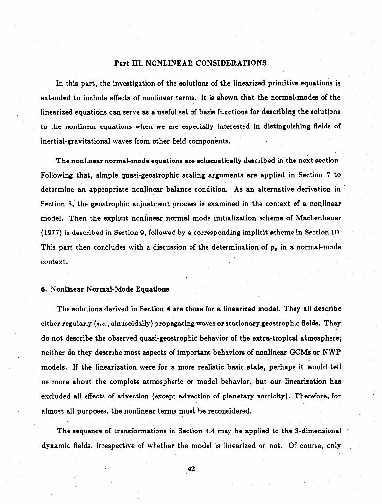
Part III. NONLINEAR CONSIDERATIONS

In this part, the investigation of the solutions of the linearized primitive equations is

extended to include effects of nonlinear terms. It is shown that the normal-modes of the

linearized equations can serve as a useful set of basis functions for describing the solutions

to the nonlinear equations when we are especially interested -in distinguishing fields of

inertial-gravitational waves from other field components.

The nonlinear normal-mode equations are schematically described in the next section.

Following that, simple quasi-geostrophic scaling arguments are applied in Section 7 to

determine an appropriate nonlinear balance condition. As an alternative derivation in

Section 8, the geostrophic adjustment process is examined in the context of a nonlinear

model. Then the explicit nonlinear normal mode initialization scheme of Machenhauer

(1977) is described in Section 9, followed by a corresponding implicit scheme in Section 10.

This part then concludes with a discussion of the determination of p. in a normal-mode

context.

6. Nonlinear Normal-Mode Equations

The solutions derived in Section 4 are those for a linearized model. They all describe

either regularly (i.e., sinusoidally) propagating waves or stationary geostrophic fields. They

do not describe the observed quasi-geostrophic behavior of the extra-tropical atmosphere;

neither do they describe most aspects of important behaviors of nonlinear GCMs or NWP

models. If the linearization were for a more realistic basic state, perhaps it would tell

us more about the complete atmospheric or model behavior, but our linearization has

excluded all effects of advection (except advection of planetary vorticity). Therefore, for

almost all purposes, the nonlinear terms must be reconsidered.

The sequence of transformations in Section 4.4 may be applied to the 3-dimensional

dynamic fields, irrespective of whether the model is linearized or not. Of course, only

42

in the linearized model will the normal-mode coefficients describe independent solutions,

and only in that model will the coefficients change in time with single frequencies given

by their corresponding eigenvalues. However, even in the original nonlinear model these

transformations are useful as an alternative description of the 3-dimensional dynamic

fields, analogous to the way in which descriptions in terms of vorticity and divergence

or potential temperature or spectral amplitude are useful for analyses which respectively

consider gradients of velocity or vertical advection of temperature or horizontal scales.

In particular, the normal-mode description is useful whenever gravity wave behavior is

to be distinguished from quasi-geostrophic behavior because with that description, the

geostrophic and gravity wave fields are represented explictly rather than implicitly as with

other formulations.

The complete nonlinear primitive equations (3.3-9) may be written schematically as

A [ru(x,y,o,,t) 1 u(x,y,,ot) Ru(, yat)- | v(x,y,o,t) = C v(x,y,,,t) a + . v(x,y,at)I , (6.1)at P(x, y,9,. t) , (a:,y,7,, t)R .(: y, ,t)

at In(p/p)(xyt) =- 6(x,y,a,t) da , (6.2)

where £ is the linear operator described earlier, and

N. =- / (u,v,o,p,t)

denotes all the nonlinear and diabatic terms (specifically all those terms excluded from

(3.13-19)). Hereafter, discussion will focus primarily on (6.1), for which we note that the

linear system forms a closed set. However, it is important to remember that determination

of the .A requires consideration of (6.2), and therefore solution of the nonlinear system

requires (6.2) also. The relationship between (6.2) and the results discussed here for (6.1)

will be deferred to Section 11.

The succession of transformations (4.49-53) may also be written schematically as[rq(t) u(x,y,,,t)9q(t = T-l(x,y,a,q) v(x,y,,t) , (6.3)gq'(t)J ,l(x,y,o,t)

43

where T - 1 represents all the successive operations in (4.49-53). Furthermore, we may

write

£T = TA, (6.4)

where A represents the algebraic operator whose elements are the frequencies of the normal

modes. Equation 6.4 is simply a reminder that A and T have been determined as the

characteristic solutions of the operator C (i.e., as solutions of the eigenvalue problem).

Applying (6.3) to all the terms in (6.1) yields the primitive equations expressed in

terms of normal modes (excluding an equation for Pa which will be considered later):

drq Nrq(r,g,g',t) (6.5)dt

dtq = -i Aq gq + Ngq(r,g,g',t) (6.6)

dgqdt= iAq g + N,,q(r,g,g',t) (6.7)

whereNrq (t) 1 u (x, y, a, t)Ngq (t)} = T (xy,,q) .(X,y, o,t) . (6.8)NgI q( t)J . Yta,)

The form of (6.5-7) is simpler than that of (6.1) only because the algebraic form of A

(which yields the algebraic factors iA) is much simpler than the integral-differential form

of L. However, if the N were to be expressed explicitly in terms of the dependent variables

r, 9, g' and Pa, they would appear much more complicated than the expressions for N/.

The equations in the form of (6.5-7) should simply be considered as a convenient linearly

transformed expression for the primitive equations. The analysis of nonlinear balance

could be performed with the equations expressed in their more usual form of (6.1), but

the results would be much less transparent.

There are only a few papers in which explicit expressions for N for atmospheric equa-

tions have been derived. These include papers by Tribbia (1979) and Thaning (1983) who

considered highly truncated shallow water equations, and Errico (1981) who considered a

horizontally periodic, two-level primitive equation, f-plane model. Although the derivation

44

is tedious for some models, the expressions are revealing in that they explicitly describe

the interactions between different scales and types of waves. Explicit expressions will not

be derived for this model here, however simple consideration of the forms of the wi reveal

that their explicit form must be e.g.,

Ngq = a cqrsrrr + ,qrrrg, + 'qrsg r g. + others, (6.9)rte

where the terms not explicitly written involve triple products of mode coefficients. These

latter occur due to the products Ta& and Tw, where 6 and w are themselves quadratic func-

tions of the prognostic fields. The a, /3, and -y are time-independent algebraic interaction

coefficients which depend on the scales m, n and H and on the types of the interacting

modes, analogous to the spectral interaction coefficients in a nonlinear spectral model (e.g.,

see Phillips, 1973). For examples of normal-mode interaction coefficients, see Errico (1981)

and Appendix B.

We should note that if Ngq(t) = 0 for all t, then the solution for g is

gq(t) = gq(0) exp(-iAqt) , (6.10)

and gravity waves are absent for all time if a linear initialization is performed. However,

clearly Ngq(t) = 0 should not be expected, since in particular, r(t) O0.

7. Scaling arguments

In this section, a simple scale analysis of the primitive equations is performed using

their expression in terms of the normal-mode coefficients. A slightly more sophisticated

scale analysis was performed by Baer (1977) and Baer and Tribbia (1977). A more detailed

scale analysis appears in Section 16. In this section, the scale analysis will be used to

derive Machenhauer's balance condition, although it is not the method which Machenhauer

himself used. His more straightforward derivation appears in the following section.

We begin by noting two observed atmospheric relationships: (1) a typical magnitude of

r is significantly larger than one for g or g' at a similar scale q; (2) the time scale (denoted by

45

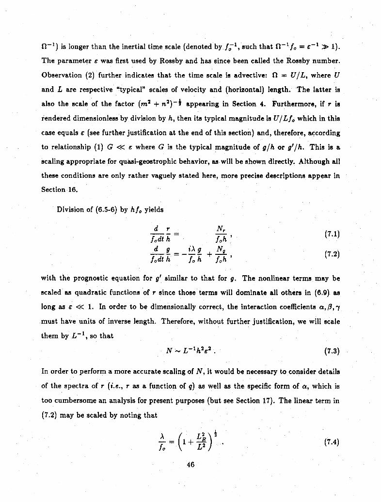
t -'l ) is longer than the inertial time scale (denoted by f 1, such that V1-fo c= > 1).

The parameter c was first used by Rossby and has since been called the Rossby number.

Observation (2) further indicates that the time scale is advective: fl = U/L, where U

and L are respective "typical" scales of velocity and (horizontal) length. The latter is

also the scale of the factor (m 2 + n2)-4 appearing in Section 4. Furthermore, if r is

rendered dimensionless by division by h, then its typical magnitude is U/Lfo which in this

case equals € (see further justification at the end of this section) and, therefore, according

to relationship (1) G << e where G is the typical magnitude of g/h or g'/h. This is a

scaling appropriate for quasi-geostrophic behavior, as will be shown directly. Although all

these conditions are only rather vaguely stated here, more precise descriptions appear in

Section 16.

Division of (6.5-6) by hfo yields

d r Nr (7.1)fodt- h (7.1)fodth foh'

d g - iAg +N 0 (7.2)fodth fo h foh '

with the prognostic equation for g' similar to that for g. The nonlinear terms may be

scaled as quadratic functions of r since those terms will dominate all others in (6.9) as

long as c << 1. In order to be dimensionally correct, the interaction coefficients a, /, y

must have units of inverse length. Therefore, without further justification, we will scale

them by L - 1 , so that

N L-lh2 c 2 . (7.3)

In order to perform a more accurate scaling of N, it would be necessary to consider details

of the spectra of r (i.e., r as a function of q) as well as the specific form of a, which is

too cumbersome an analysis for present purposes (but see Section 17). The linear term in

(7.2) may be scaled by noting that

f = (~~~~~~1 + L ) *(7.4)~oo -1+~-

46

With these scalings and restricting attention to scales such that << L L 2 « L 1, the

scaling of the respective terms in (7.1-7.2) is

[21 d r 21 Nr (7.5)dt h

[E = -[G] i + [ 2]No (7.6)

where the scales are shown in brackets. The additional restriction on LR/L is necessary to

simplify the analysis, so that LR/L 1, and ensures that the considered horizontal scales

are not too dissimilar to the radius of deformation.

For E << 1 and G «<< e, the simple scaling of (7.5-6) indicates that the time tendency

term for g typically has a smaller magnitude than either the linear or nonlinear term in

(7.8). In other words, through second order in r,

0 ~ -iAg + N 0 (r) . (7.7)

The linear term must approximately balance (i.e., cancel) the nonlinear term, by having

similar magnitude but opposite sign. In order for the dynamics to be consistent with

observations, (7.7) must apply. In Section 10, (7.7) will be shown to correspond to

scale-dependent forms of both the quasi-geostrophic omega-equation and nonlinear balance

equation. If the scaling arguments are applied rigorously (e.g., as by Baer and Tribbia,

1977), the accuracy of (7.7) increases as e decreases, since the corrections to (7.7) are an

order e smaller than the retained terms.

If the asymptotic relation (7.7) is replaced by an equality, then (7.7) becomes a

diagnostic equation relating g to r. In contrast, at the same order of accuracy, the nonlinear

prognostic equation for r remains as (7.1) except with Nr determined from r alone. Given

the set of values of r at any time, the g can be approximately determined using (7.7) if

the scaling is appropriate for all time and if E is sufficiently small. These properties will

be examined in greater detail in Section 17.

Some further explanation should be given for relating the typical magnitude of r/h

to E. Actually, under quasi-geostrophic conditions, this is only accurate for scales where

47

L is similar to LR. The value of c may properly be related to the scaling of £/fo since

~ U/L. If g << r, then the near geostrophic balance implies

fo ~ -((m' + n 2 )p, (7.8)

where m 2 + n2 is associated with the scale L - 2 . Substitution of (7.8) into the definition

of r as a scaled linearized potential vorticity (4.40) yields (after manipulation)

r L2

using identities such as (7.4) and (5.2).

8. Dynamics of Nonlinear Model

The simple scaling arguments in Section 7 suggest that for weak flows (i.e., e <« 1)

and advective time scales, an approximate balance necessarily exists between the linear and

dominant nonlinear terms in the prognostic equation for a gravitational mode amplitude.

Here we describe this result as a consequence of nonlinear geostrophic adjustment. This

process will be described more thoroughly in Section 18, but here we wish to provide a

basis for nonlinear normal-mode initialization.

For this purpose, we may consider the prognostic equation for a gravitational mode

coefficient to have the formdgd= = -i A g + Ng(t), (8.1)

where a scale q is to be understood, and here we are only considering that Ng is some

specified function of t. Actually of course, Ng is a function of all the mode coefficients,

including perhaps this g itself, but each coefficient may itself by considered as a function

of t. Naturally, N can only really be determined if its functional dependence on the

mode coefficients or corresponding 3-dimensional fields is given. Therefore consideration

of N as only N(t) is not useful for prediction, although it is useful for understanding the

relationships between the tendency, linear, and nonlinear terms in general and regarding

their balance in particular.

48

Machenhauer (1977) examined values of N. as a function of t as output by a numerical

model. He observed that over short, inertial periods, Ng had a relatively large stationary

component. In other words, it was approximately constant over such time periods. This

observation is consistent with the scale analysis of the previous section which revealed

that Ng was primarily determined by r, which itself is prognostically governed by terms

nonlinear in r. This latter result implies that the time scale of r is primarily advective,

and therefore by further implication, that the primary time scale of Ng is advective. These

assertions will be examined in greater detail in Part V. Here we will take them as observed

facts. However, we will also consider that Ng(t) is not stationary in time, but instead has

the harmonic form

Ng (t) - N e-tl (8.2)

where N is a time-independent amplitude and |[g << AIt. The latter condition ensures

that the forcing indeed has a time scale longer than that of the linear wave.

Given a harmonic Ng, the solution of (8.1) may be readily written as

g(t) = [g (0) - - i e e' + i - i* (8.3)[ t A -]u v /

From (8.3) we note that g(t) has two components. One has the frequency of a linear

inertial-gravitational wave, and the other has that of the forcing. The amplitude of the

former component depends on both the initial condition and forcing magnitude; the latter

depends only on the forcing magnitude and the difference between the linear and forcing

frequencies. The two components are sometimes called the fast and slow components

respectively (or the free and forced components). Implications of the properties of (8.3)

will be discussed in greater detail in Part V, but some important implications regarding

initialization will be made here also.

In order to remove the fast component from the solution it is necessary to specify

g(0)= i . (8.4)

49

If, additionally, / is approximated by zero in (8.4), then (8.4) may be replaced by

(0) i ' (8.5)

or equivalently

g(0)= NN (8.6)

The approximation A = 0 in (8.4) is appropriate since << « A has been assumed. Equation

(8.6) is further equivalent to the condition

dgd- =0 at t = 0. (8.7)

The approximation s = 0 in (8.4) is also equivalent to the approximation of ignoring the

time tendency of the forced component of the solution (i.e., that given by the last term in

(8.3)), since that tendency is equal to

d (Ng (t)) (Ng(t)) (8.8)dt-i i - i, = A - t/i1 8i

The condition (8.6) expresses a balance between the linear inertial-gravitational force

and the nonlinear advection, expressed in terms of normal-mode coefficients. Condition

(8.7) is known as Machenhauer's (1977) balance condition. Since A ~ 0 generally, this

condition for the removal of fast solutions is necessarily approximate. However, as long

as |^|<< « A, the approximation appears suitable. Also, the more exact relationship (8.4)

suggests higher order diagnostic balance conditions. These will be discussed further in

Section 19, and generalized expressions for (8.1) and (8.4) in terms of a continuum of

frequencies will be discussed in Section 18. At this point we will simply add that (8.7)

holds also if the forcing has many associated frequencies, as long as its corresponding power

spectrum is sufficiently red and if additionally there is sufficient quasi-linear damping or

other mechanisms to prevent infinite resonant responses.

Simply setting g(0) = 0 (i.e., a linear initialization) does not remove fast solutions at

later times. In fact, values g + 0 occur on the fast time scale. Initially, the fast component

50

solution has opposite phase and identical magnitude with respect to the forced component,

but at later times the phase of the fast component changes more rapidly than that of the

slow component, and cancellation no longer occurs. The solution 8.4 also reveals why

linear initialization is sometimes successful: if an analyzed value of g(0) is much larger

than its forced component, then replacing 9(0) by 0 reduces the subsequent amplitude of

the fast component to the magnitude of the forced component.

9. Machenhauer's Normal-Mode Balance Scheme

On the basis of (8.7), Machenhauer's (1977) scheme is to set

0 = -iAg + Ng (r,g',gt) at t = 0 (9.1)

for some set of gravitational modes, with a corresponding condition for g9'. If only adia-

batic contributions to the tendencies are considered, then the scheme is called adiabatic;

otherwise it is called diabatic. The selection of a specific set of modes for application of

(9.1) remains a topic of some debate and necessarily involves many theoretical as well

as practical considerations. Some aspects will be discussed in Sections 15 and 17. The

coefficients for the rotational modes are usually unaltered from their analyzed values.

Machenhauer's condition (9.1) is not entirely consistent with a quasi-geostrophic e-

parameter scale analysis of the primitive equations (Section 7). Remember there, it was

asserted that through second order,

0 =-iAg + N(r), (9.2)

whereas (9.1) as stated has no approximation of the nonlinear terms; i.e., (9.1) includes

terms involving products of r and g as well as g and g (cf., 6.9). However, according to the

scaling in Section 7, these additional nonlinear terms are of the same typical scale as the

neglected tendency term. In Section 17, a detailed scale analysis will show that this simple

scaling argument is not entirely accurate and that for some gravitational modes the terms

51

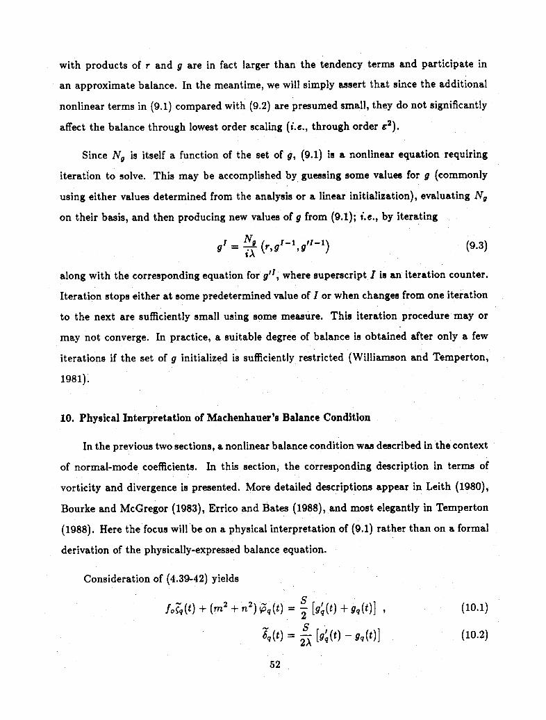
with products of r and g are in fact larger than the tendency terms and participate in

an approximate balance. In the meantime, we will simply assert that since the additional

nonlinear terms in (9.1) compared with (9.2) are presumed small, they do not significantly

affect the balance through lowest order scaling (i.e., through order €2 ).

Since Ng is itself a function of the set of g, (9.1) is a nonlinear equation requiring

iteration to solve. This may be accomplished by guessing some values for g (commonly

using either values determined from the analysis or a linear initialization), evaluating Ng

on their basis, and then producing new values of g from (9.1); i.e., by iterating

9g Ng (r, 9gl 9,1'= N r,0 - 1,^- 1 , (9.3)i

along with the corresponding equation for g'1 , where superscript I is an iteration counter.

Iteration stops either at some predetermined value of I or when changes from one iteration

to the next are sufficiently small using some measure. This iteration procedure may or

may not converge. In practice, a suitable degree of balance is obtained after only a few

iterations if the set of g initialized is sufficiently restricted (Williamson and Temperton,

1981).

10. Physical Interpretation of Machenhauer's Balance Condition

In the previous two sections, a nonlinear balance condition was described in the context

of normal-mode coefficients. In this section, the corresponding description in terms of

vorticity and divergence is presented. More detailed descriptions appear in Leith (1980),

Bourke and McGregor (1983), Errico and Bates (1988), and most elegantly in Temperton

(1988). Here the focus will be on a physical interpretation of (9.1) rather than on a formal

derivation of the physically-expressed balance equation.

Consideration of (4.39-42) yields

2 ^ ^+ n 2 )^^^ ] (10.1)fo(t) + (m + ) (t) - [g(t) + 9q (t)] (10.1)

6q(t) = S [gq(t) - gq(t)] (10.2)

52

for every scale q. Similarly,

Therefore, the Machenhauer balance condition (8.7) or (9.1) applied to gq and gg simultaneouslyf o + +(M +n 2+n2) d?=0 O(10.5)

dt 2'd '+

d-t =0 ° (10.6)

at each scale q.

Further enlightment occurs when we consider that

dt q ^-^~~~~+A Sq ' ~(10.7)

t = foq + (m 2 + n2 ) -q + Ns, (10.8)

d.q

The N represent all the nonlinear terms which affect the subscripted field at scale q.

Equations 10.7-9 are simply the primitive equations (excluding the explicit equation for

the surface pressure tendency) described in terms of vorticity, divergence, and pseudo-

geopotential at a spatial scale q, with the nonlinear terms present but not explicitly

described. Substitution of (1+ N0.7-9) into (10.5-6) yields

foq + (m 2 + 2) +N^ = (10.10)

-[f+O g + m 2 + n 2 + foq + ( 2 + n2 ) = 0 (10.11)

for the balance condition at scale q.

In this section until now we have considered the balance equations only in terms of

spectral coefficients (as indicated by the tilde). In order to consider their corresponding

53

form in physical space, we will simply consider that the factors gH and m 2 + n2 which

appear in (10.10-11) correspond to the respective operators r and -(I + I) in physical

space acting on scale q. Also, we use the fact that different scales may be superimposed

so that (10.10-11) are equivalent to

for - V2p + N6 = 0, (10.12)

-[fo - rV 2] 6 + foNC - V 2N = o, (10.13)

where

92 a2

2x 2

Equation 10.12 is a form of the nonlinear balance equation. A difference between

its usual form and (10.12) is that no approximations have been made for the nonlinear

terms: usually N 6 is further simplified to exclude any terms which involve the divergent

component of the wind. A further difference between (10.12) and the usual nonlinear

balance equation is that the usual one is typically solved by specifying either p or ~,

whereas (10.12) is typically solved by constraining the rotational mode coefficients, which

is equivalent to constraining

P = f-f 1or-p (10.14)

which is a form of scaled linearized potential vorticity. How (10.14) may be combined with

(10.12) to yield an equation of a form which facilitates solution is described in Section 14.

Equation 10.13 is a form of the quasi-geostrophic w-equation, except expressed here in

terms of divergence rather than w, which are simply related according to (3.8). More usual

expressions of the quasi-geostrophic w-equation also have both sides of (10.13) operated by

a differential expression equivalent to r - 1. Also, like for the nonlinear balance equation,

they have further approximation to the nonlinear terms. At many scales, these further

approximations change the N only slightly, although at other scales the alterations may

yield significantly different results (See Section 17 for further discussion of this point).

54

Another significant difference between the balance condition (10.12-13) and its more

common form is that when expressed in terms of normal modes, it is natural to apply

the condition only to selected vertical and horizontal scales. This should be contrasted

with previous applications of the nonlinear balance condition and quasi-geostrophic omega

equations which typically were applied indiscriminately at all scales (for an exception,

see e.g., Barker, 1982). Since, as will be shown in Section 17, the appropriateness of

Machenhauer's balance condition actually is strongly scale dependent, the indiscriminate

application of (10.12-13) should be avoided and will likely yield unrealistic results within

some range of scales.

Finally, it should be noted that (10.12-13) should be applied simultaneously, a fact

known for at least 30 years (see Phillips (1960)). Application of either separately for the

purpose of initialization is analogous to adjusting only half the wave structure.

11. Determination of pA

In Sections 5-10, the adjustment process for the mass field has been described in terms

of that for the pseudo-geopotential field. Both the temperature and surface pressure fields

undergo adjustment since (p = so(T, p.). In order to partition the adjustment between the

T and p. fields, an additional relation is required since the number of degrees of freedom

for T and p. correspond to one more horizontal field than that for < (which has the same

degree of freedom as T). An additional relation may be obtained from reconsideration

of the tendency equation for p. (Andersen, 1977) or from some variational consideration

(Daley, 1979).

The necessity for an additional relation is most easily seen in the case of a vertically

discrete model for which both yp and T are defined on K-independent a-levels and p, is

defined on an additional o level (. e., the surface a = 1). The adjustment process described

thus far provides knowledge of K values of p at each horizontal location (one value for

each level). However, we wish to determine K values of T (one for each of the same levels)

55

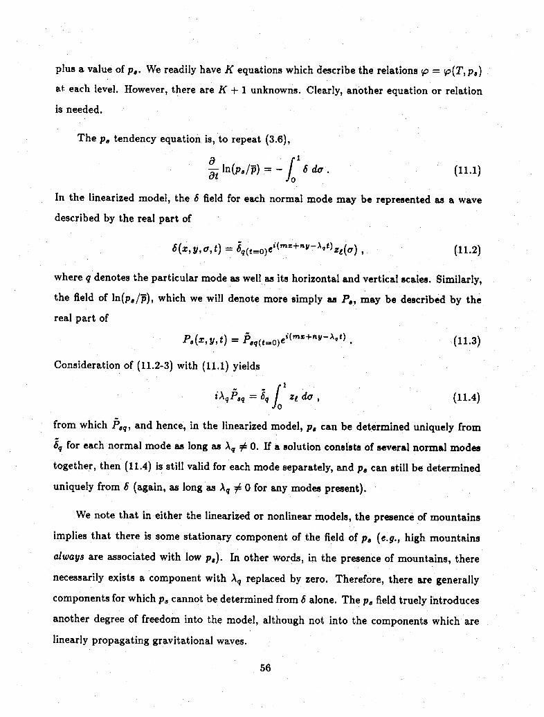
plus a value of p,. We readily have K equations which describe the relations p = p(T, pa)

at each level. However, there are K + 1 unknowns. Clearly, another equation or relation

is needed.

The pa tendency equation is, to repeat (3.6),

ln(p,/p) = - 6 da (11.1)

In the linearized model, the 6 field for each normal mode may be represented as a wave

described by the real part of

6(x, y, a, t) = 6q(t=o)ei(m:+h^ -t)zt( a ) , (.11.2)

where q denotes the particular mode as well as its horizontal and vertical scales. Similarly,

the field of ln(p,/p), which we will denote more simply as Pa, may be described by the

real part of

P(x, y, t) = Pvq(t=o)et (mz+ny- A t) (11.3)

Consideration of (11.2-3) with (11.1) yields

iAqPaq = 6 q j Zd , (11.4)

from which Paq, and hence, in the linearized model, p, can be determined uniquely from6q for each normal mode as long as Aq #0. If a solution consists of several normal modes

together, then (11.4) is still valid for each mode separately, and p. can still be determined

uniquely from 6 (again, as long as Aq # 0 for any modes present).

We note that in either the linearized or nonlinear models, the presence of mountains

implies that there is some stationary component of the field of p. (e.g., high mountains

always are associated with low pa). In other words, in the presence of mountains, there

necessarily exists a component with Aq replaced by zero. Therefore, there are generally

components for which p, cannot be determined from 6 alone. The p, field truely introduces

another degree of freedom into the model, although not into the components which are

linearly propagating gravitational waves.

56

In the nonlinear model, (11.1) is valid, but (11.2-3) and hence (11.4) are invalid because

each mode may be associated with several (or a continuum of) frequencies, not only its

natural frequency Aq. Therefore, in such a model or in the atmosphere it represents,

it is generally impossible to uniquely determine p. from 6 with or without mountains,

although for any components acting as free (normal mode) waves, (11.4) can be used to

relate the fields of those components alone. Therefore, (11.4) remains useful for relating

p. and 6 fields associated with propagating gravitational waves. In particular, it can be

used for the initialization of such waves, as long as it is applied only to freely-propagating

components. In a precise sense, there are no truely free components (all are coupled through

the nonlinearity), but (11.4) can be considered an appropriate approximation when applied

to the unbalanced components of gravitational modes.

In NNMI procedures, usually adjustments to p. are related to adjustments to p by

considering both (11.4) and, according to (3.26),

iA p(x,y,a,t) = r6(x,y,a,t) (11.5)

for each normal mode (in the linearized model). Together, these yield the relation

Paq = 3q rT ze d . (11.6)o

Furthermore, assuming (11.6) remains valid for a superposition of modes,

P,= r-1 <pda. (11.7)

Equation 11.7 is simpler to impliment than is (11.4) in that it can be applied in physical

space rather than mode space and the A no longer explicitly appear, thereby reducing

computational expenses.

Once ps is determined from (11.4) or (11.7), T' can be determined from

' = ln(p/p)Ina - Rl ' (11.8)

57

which is the differentiated form of (3.22). However, in practice, there are sometimes

substantial difficulties with this use of (11.8). This difficulty occurs with many of the usual

finite difference approximations for the hydrostatic equation, and regards the sensitivity

of the determination of T' to small errors or inappropriate specification of P., as discussed

next.

The sensitivity of values of T' to specification of p., given a field of .p and using (11.8),

is expressed by

( anp) Tn. (11.9)

Note that for an isothermal basic state, T" is not related to p, according to (11.8), but p,

instead only determines the barotropic structure of p.

The result in a vertically discrete model may be very different than (11.9), however,

depending on the precise specification of the form of the hydrostatic equation applied to

the lowest model level. Consider the simple finite difference form

PK = + RTK In (pa/p) - RTK In TaK,

Rpk = Pk+ .+ R (Tk - Tk+l) In (Pe/P) + 2 (Tk + Tk+1) (In k+ - lnak)- 1 for k < K ,

(11.10)

where the subscript K refers to the value at the lowest model level, K - 1 to the next

highest level, etc. The form (11.10) is similar to that for the NCAR CCM and PSU/NCAR

MM4. For (11.10), the sensitivity of the determination of TK from p., given values of o is

( lnp - lnaK

even in an isothermal atmosphere, unlike (11.9). Note that since

InK ~ 1 -aK as K - 1, (11.12)

the sensitivity increases as the depth (i.e., 1 - OK) of the lowest layer decreases. Also note

that for an isothermal basic state

(aLn) p. - =-.) fork<K, (11.13)c9lIn pf, 9p in np

58

which follows from the second equation in (11.10). In other words, at some horizontal

location, an inaccurate or inappropriate specification of In pa yields an inaccurate vertical

temperature structure which changes sign between each vertical level and has a magnitude

approximately proportional to TK(1 - aK) 1 as well as to the error in Inp,.

Since the determination of adjustments of pa using (11.8) is only an approximation

in a nonlinear model, the use of finite-difference approximations such as (11.10) to (11.8)

may create unacceptable values for the determination of T' in numerical (i.e., vertically

discrete) models. This may especially occur for models whose lowest level is very shallow.

In those cases, some other determination of p, should be used. One such alternate method

is the variational determination suggested by Daley (1979). He defines a quadratic measure

of the changes produced for the T' and pd fields at each horizontal location, and then seeks

the set of values which minimize that measure given the specified changes in p. For

further description, the reader should consult Daley (1979). His method has been used

satisfactorily in many cases (e.g., see Errico and Bates, 1988).

59

Part IV. APPLICATION OF NNMI TO NUMERICAL MODELS

In this part, some aspects of the application of NNMI to global and regional numerical

models are discussed. Since details of such applications are provided elsewhere (e.g.,

Anderson, 1977; Daley, 1979; Temperton and Williamson, 1981; Williamson and Temperton,

1981; Briere, 1982; Bourke and McGregor, 1983; Du Vachat, 1986; Errico, 1987; Errico

and Eaton, 1987; Wergen, 1987; Errico and Bates, 1988; Temperton, 1988), here attention

is focused on general application, differences between analytic and numerical methods, and

aspects not covered or highlighted in most literature. The models to which the methods

are applied are a global spectral model and a regional mesoscale model.

In Section 12, the vertical modes of versions of both models are presented and their

characteristics described along with the method for obtaining them. Machenhauer's tech-

nique applied to a global spectral model is briefly described in Section 13 along with some

discussion of the convergence of the iterative scheme for solving the NNMI equations and

an example of the noise reduction in subsequent forecasts. Similar results are presented in

Section 14 for the regional model. This part concludes with a discussion of the criteria for

selecting scales to initialize and the consideration of variational methods in Section 15.

The global model used as an example in this report is version 1 of the NCAR

Community Climate Model (designated CCM1; Williamson et al., 1987). The particular

version used here has rhomboidal spectral truncation at zonal wavenumber 15, correspond-

ing to a Gaussian grid of 48 longitudes by 40 latitudes. The dynamic fields are defined on

12 unequally-spaced levels in the vertical, excluding fields at the surface. Diabatic physics

includes moist convective adjustment, precipitation from convectively stable but saturated

layers, solar and infrared radiative fluxes which interact with model generated clouds,

and both vertical and horizontal diffusion. Numerically, the model uses a semi-implicit

integration scheme with a time filter to limit time-computational modes. The CCM1 is

used primarily for climate studies, but it is also used for NWP studies. Its associated

60

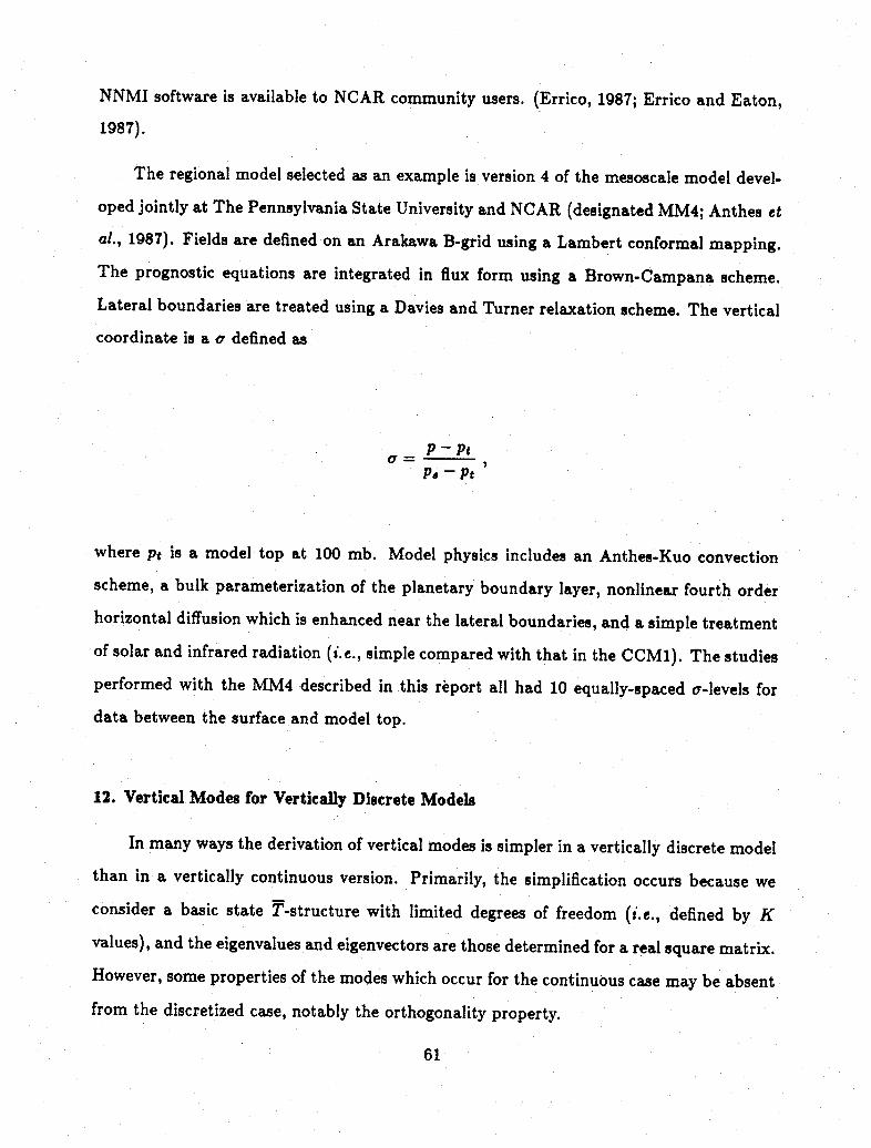
NNMI software is available to NCAR community users. (Errico, 1987; Errico and Eaton,

1987).

The regional model selected as an example is version 4 of the mesoscale model devel-

oped jointly at The Pennsylvania State University and NCAR (designated MM4; Anthes et

al., 1987). Fields are defined on an Arakawa B-grid using a Lambert conformal mapping.

The prognostic equations are integrated in flux form using a Brown-Campana scheme.

Lateral boundaries are treated using a Davies and Turner relaxation scheme. The vertical

coordinate is a a defined as

P - PtP- Pt

where Pt is a model top at 100 mb. Model physics includes an Anthes-Kuo convection

scheme, a bulk parameterization of the planetary boundary layer, nonlinear fourth order

horizontal diffusion which is enhanced near the lateral boundaries, and a simple treatment

of solar and infrared radiation (i.e., simple compared with that in the CCM1). The studies

performed with the MM4 described in this report all had 10 equally-spaced a-levels for

data between the surface and model top.

12. Vertical Modes for Vertically Discrete Models

In many ways the derivation of vertical modes is simpler in a vertically discrete model

than in a vertically continuous version. Primarily, the simplification occurs because we

consider a basic state T-structure with limited degrees of freedom (i.e., defined by K

values), and the eigenvalues and eigenvectors are those determined for a real square matrix.

However, some properties of the modes which occur for the continuous case may be absent

from the discretized case, notably the orthogonality property.

61

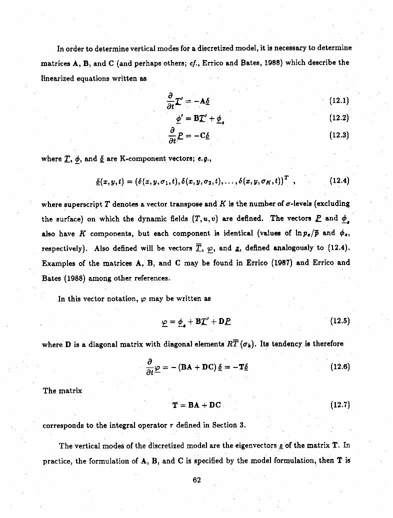
In order to determine vertical modes for a discretized model, it is necessary to determine

matrices A, B, and C (and perhaps others; cf., Errico and Bates, 1988) which describe the

linearized equations written as

'=-A6 (12.1)at -_= BT' + (12.2)

t P=-CE (12.3)

where T, and 6 are K-component vectors; e.g.,

(y, t) = (6(z,y, a, t),6(, y, 2 , t),...,6(, aK, t)) , (12.4)

where superscript T denotes a vector transpose and K is the number of a-levels (excluding

the surface) on which the dynamic fields (T,u,v) are defined. The vectors P and o

also have K components, but each component is identical (values of Inpo/p and 4X,

respectively). Also defined will be vectors 3, _, and _ , defined analogously to (12.4).

Examples of the matrices A, B, and C may be found in Errico (1987) and Errico and

Bates (1988) among other references.

In this vector notation, p may be written as

o= < + BT' + DP (12.5)

where D is a diagonal matrix with diagonal elements RT (ak). Its tendency is therefore

a-- = =- (BA + DC) 6 =-T (12.6)

The matrix

T=BA +DC (12.7)

corresponds to the integral operator r defined in Section 3.

The vertical modes of the discretized model are the eigenvectors z of the matrix T. In

practice, the formulation of A, B, and C is specified by the model formulation, then T is

62

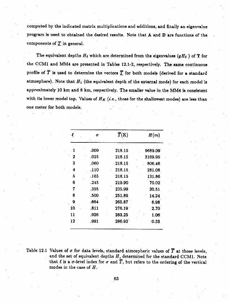
computed by the indicated matrix multiplications and additions, and finally an eigenvalue

program is used to obtained the desired results. Note that A and D are functions of the

components of T in general.

The equivalent depths Hi which are determined from the eigenvalues (gHi ) of T for

the CCM1 and MM4 are presented in Tables 12.1-2, respectively. The same continuous

profile of T is used to determine the vectors T for both models (derived for a standard

atmosphere). Note that Hi (the equivalent depth of the external mode) for each model is

approximately 10 km and 8 km, respectively. The smaller value in the MM4 is consistent

with its lower model top. Values of HK (i.e., those for the shallowest modes) are less than

one meter for both models.

ear T(K) H(m)

1 .009 218.15 9689.092 .025 218.15 3169.953 .060 218.15 806.464 .110 218.15 281.085 .165 218.15 131.866 .245 219.90 70.027 .355 235.99 30.518 .500 251.89 14.249 .664 265.87 6.98

10 .811 276.19 2.7011 .926 283.25 1.0612 .991 286.93 0.33

Table 12.1 Values of o for data levels, standard atmospheric values of T at those levels,and the set of equivalent depths H, determined for the standard CCM1. Notethat I is a a-level index for a and T, but refers to the ordering of the verticalmodes in the case of H.

63

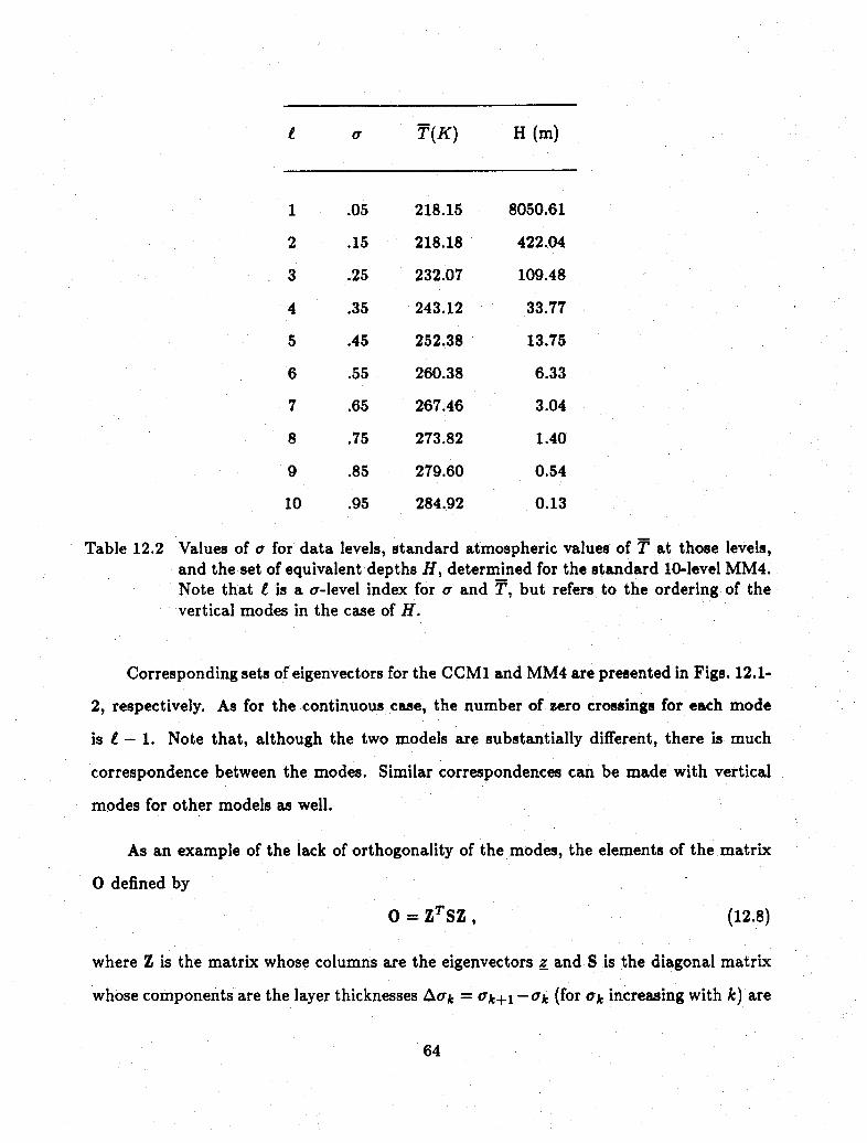
t a T(K) H (m)

1

2

3

4

5

6

7

8

9

10

.05

.15

.25

.35

.45

.55

.65

.75

.85

.95

218.15

218.18

232.07

243.12

252.38

260.38

267.46

273.82

279.60

284.92

8050.61

422.04

109.48

33.77

13.75

6.33

3.04

1.40

0.54

0.13

Table 12.2 Values of a for data levels, standard atmospheric values of T at those levels,and the set of equivalent depths H, determined for the standard 10-level MM4.Note that t is a a-level index for a and T, but refers to the ordering of thevertical modes in the case of H.

Corresponding sets of eigenvectors for the CCM1 and MM4 are presented in Figs. 12.1-

2, respectively. As for the continuous case, the number of zero crossings for each mode

is t - 1. Note that, although the two models are substantially different, there is much

correspondence between the modes. Similar correspondences can be made with vertical

modes for other models as well.

As an example of the lack of orthogonality of the modes, the elements of the matrix

0 defined by

0 = ZTSZ, (12.8)

where Z is the matrix whose columns are the eigenvectors z and S is the diagonal matrix

whose components are the layer thicknesses Aak = ak+l -- k (for ak increasing with k) are

64

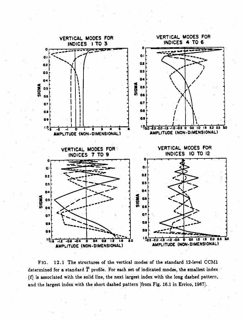
VERTICAL MODES FORINDICES I TO 3

AMPLITUDE (NON-DIMENSIONAL)

VERTICAL MODES FORINDICES 7 TO 9

AMPLITUDE (NON-DIMENSIONAL)

VERTICAL MODES FORINDICES 4 TO 6

I0K

AMPLITUDE (NON-DIMENSIONAL)

VERTICAL MODES FORINDICES 10 TO 12

oe

05ib

AMPLITUDE (NON-DIMENSIONAL)

FIG. 12.1 The structures of the vertical modes of the standard 12-level CCM1

determined for a standard T profile. For each set of indicated modes, the smallest index

(1) is associated with the solid line, the next largest index with the long dashed pattern,

and the largest index with the short dashed pattern [from Fig. 16.1 in Errico, 1987].

I(0

41aaU,

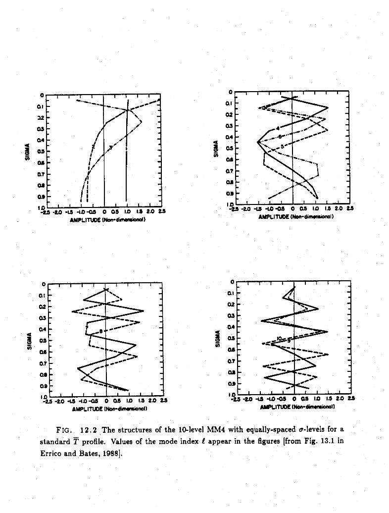
5)

a& _ -&Iv~t munq n ng rA 2-

AMPLITUDE d(No) AMPLITUE (Nofdi

AMPLITUDE (NNoon)ieOl)

FIG. 12.2 The structures of the 10-level MM4 with equally-spaced 7-levels for a

standard T profile. Values of the mode index e appear in the figures [from Fig. 13.1 in

Errico and Bates, 1988].

C

.4

u)

ot

a0

.5-W -- --

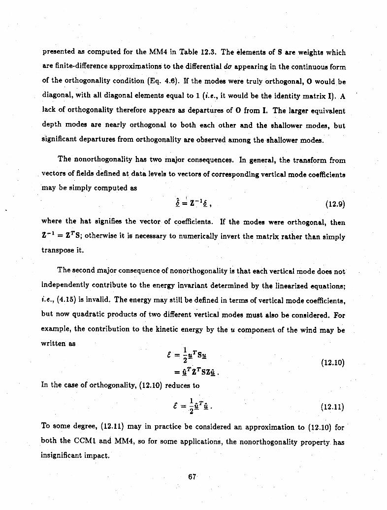
presented as computed for the MM4 in Table 12.3. The elements of S are weights which

are finite-difference approximations to the differential da appearing in the continuous form

of the orthogonality condition (Eq. 4.6). If the modes were truly orthogonal, 0 would be

diagonal, with all diagonal elements equal to 1 (i.e., it would be the identity matrix I). A

lack of orthogonality therefore appears as departures of 0 from I. The larger equivalent

depth modes are nearly orthogonal to both each other and the shallower modes, but

significant departures from orthogonality are observed among the shallower modes.

The nonorthogonality has two major consequences. In general, the transform from

vectors of fields defined at data levels to vectors of corresponding vertical mode coefficients

may be simply computed as

~_ =Z- 1 E, (12.9)

where the hat signifies the vector of coefficients. If the modes were orthogonal, then

Z -1 = ZTS; otherwise it is necessary to numerically invert the matrix rather than simply

transpose it.

The second major consequence of nonorthogonality is that each vertical mode does not

independently contribute to the energy invariant determined by the linearized equations;

i.e., (4.15) is invalid. The energy may still be defined in terms of vertical mode coefficients,

but now quadratic products of two different vertical modes must also be considered. For

example, the contribution to the kinetic energy by the u component of the wind may be

written as1

= -UTSu2 (12.10)

= TZSZu

In the case of orthogonality, (12.10) reduces to

1ATA£ __ = Ur. (12.11)

2= a.

To some degree, (12.11) may in practice be considered an approximation to (12.10) for

both the CCM1 and MM4, so for some applications, the nonorthogonality property has

insignificant impact.

67

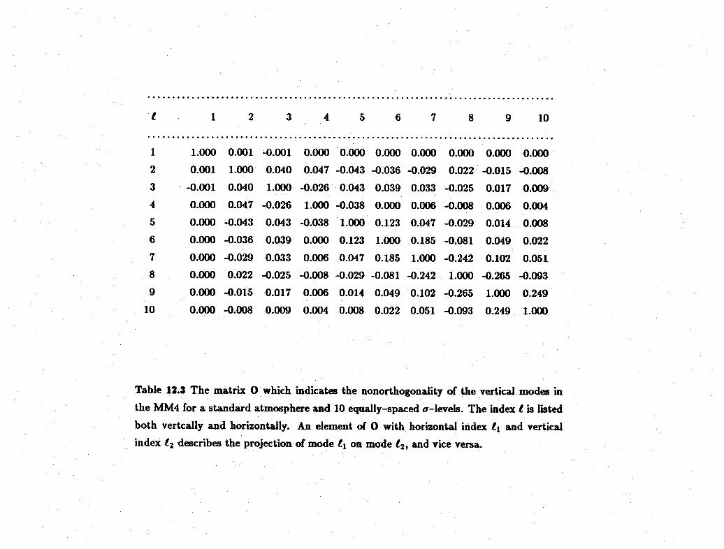
1 2 3 4 5 6 7 8 9 10

1 1.000 0.001 -0.001 0.000 0.000 0.000 0.000 0.000 0.000 0.000

2 0.001 1.000 0.040 0.047 -0.043 -0.036 -0.029 0.022 -0.015 -0.008

3 -0.001 0.040 1.000 -0.026 0.043 0.039 0.033 -0.025 0.017 0.009

4 0.000 0.047 -0.026 1.000 -0.038 0.000 0.006 -0.008 0.006 0.004

5 0.000 -0.043 0.043 -0.038 1.000 0.123 0.047 -0.029 0.014 0.008

6 0.000 -0.036 0.039 0.000 0.123 1.000 0.185 -0.081 0.049 0.022

7 0.000 -0.029 0.033 0.006 0.047 0.185 1.000 -0.242 0.102 0.051

8 0.000 0.022 -0.025 -0.008 -0.029-0.081 -0.242 1.000 -0.265 -0.093

9 0.000 -0.015 0.017 0.006 0.014 0.049 0.102 -0.265 1.000 0.249

10 0.000 -0.008 0.009 0.004 0.008 0.022 0.051 -0.093 0.249 1.000

Table 12.3 The matrix 0 which indicates the nonorthogonality of the vertical modes in

the MM4 for a standard atmosphere and 10 equally-spaced or-levels. The index t is listedboth vertcally and horizontally. An element of 0 with horizontal index tl and verticalindex t2 describes the projection of mode t4 on mode t2, and vice versa.

t

13. Explicit NNMI

When NNMI is expressed explicitly in terms of normal-mode coefficients, Temperton

(1988) has appropriately named it explicit NNMI. The usual methodology for iterating the

nonlinear explicit equations is

g+1 = gq + Ag (13.1)

for some set q of modes, where superscript I is an iteration counter and

=- d , (13.2)

where the tendency is computed as

d -t = i q g+ Ngq (r, 1 , g ). (13.3)

The form of (13.2) is determined by substituting (13.1) into (9.3) and then using (13.3).

Typically the initial value (g ) either is the value of gq as obtained by projection of analyzed

data or is gq = 0 (i.e., a linear initialization). Typically, (13.1-2) are iterated for a fixed

number of times (typically through I < 3), although it is possible to iterate until some

condition such as

1t1 < C (13.4)

is achieved for some prespecified value of eC. The resulting solutions will depend on

the initial values because the equations are nonlinear, however for many applications the

resulting differences may be small. The reason for this is discussed next.

Following the analysis of Errico (1984a), the nonlinear equation which Machenhauer's

(1977) scheme is attempting to solve may be expressed as

g = -iA- 1 [r + Rg + b (g)] , (13.5)

where

69

g is a vector whose components are the gq to be initialized,

A is the diagonal matrix whose diagonal elements are the frequencies Aj of the corre-

sponding gravitational modes,

r is a vector whose components are the forcings of gq by the interaction of all the

rotational modes,

R is a matrix which depends on the rotational mode amplitudes such that Rg describes

the forcing of the gravitational modes by the explicit interaction of rotational and

gravitational modes, and

b is a vector whose components are the forcings of gq by all the nonlinear interactions

of the gravitational modes.

Equation (13.5) may be considered quasi-linear, in the sense that

(r)q << (Rg)q << (b)q (13.6)

for most sets of gravitational modes for real-atmospheric values.

Errico (1984a) shows that the lack of convergence of (13.1-2) is usually due to the

presence of the quasi-linear term Rg rather than the nonlinear b, although when an

atmosphere with larger than realistic values of the Rossby number is considered, then

the effect of b becomes more significant (Thaning, 1983). Errico (1984a) also shows that if

b is excluded, then the solution to (13.1-2) is independent of the initial value of g as long

as (13.1-2) converges, and furthermore, that convergence is completely determined by the

eigenvalues of A. R. Other discussions of the convergence properties of (13.1-2) appear in

Ballish (1982) and Rasch (1985a). A scheme for solving the Machenhauer balance condition

(9.1) which has better convergence properties than the scheme (13.1-2) is presented in

Rasch (1985b).

70

A frequently used measure of the convergence of (13.1-2) is the scalar

Bl = 1 dgt dg (13.6)B 1= - .9 -rff- -^(13.6)2 Z dt dtgq

q

For the modes initialized, B should converge to zero as I increases. For examples of suchconvergence (or lack thereof) see Williamson and Temperton (1981), Kitade (1983), or mostother papers regarding implementation of Machenhauer's (1977) scheme. Other measures

of convergence are presented in Errico (1983), Rasch (1985b), or Errico and Eaton (1987).

A result of NNMI applied to a global forecast model is presented in Fig. 13.1 whereseveral time series in forecasts begun from analyzed fields with and without NNMI (re-

spectively indicated by dashed and solid lines) are shown for selected fields at one point in

the model. This example is taken from Errico and Eaton (1987), where the NCAR CCMwas used starting from a ECMWF analysis for 16 January 1979, and the NNMI scheme

used Rasch's (1985b) iteration method applied to all gravitational modes satisfying theconditions t < 6 and P < 36 hours. The figure for p,(t) is the same as in Fig. 1.1.

Note in Fig. 13.1 that "noise" has been reduced by NNMI in the fields of p., T, and 6,

and the 5-day forecast of f has been changed very little. Results for other model points

appear qualitatively similar, indicating that the NNMI procedure has successfully reduced

gravitational noise without significantly affecting the slower forecast components during

the 5-day period.

It is noteworthy that an oscillation of the a field remains with an approximate period

of 10 hours. This oscillation may be due to slower quasi-geostrophic dynamics during the

24 hours shown, or it may be due to propagating internal gravitational waves at vertical

or horizontal scales which the NNMI has ignored. Since 6 describes an internal vertical

velocity, it may be expected to be sensitive to the presence of internal gravitational waves

(for further discussion of this point, see Errico and Williamson, 1988)

Explicit NNMI has been applied to most global numerical forecast models. It has

also been applied to several regional (i.e., limited-area) numerical forecast models (e.g.,

71

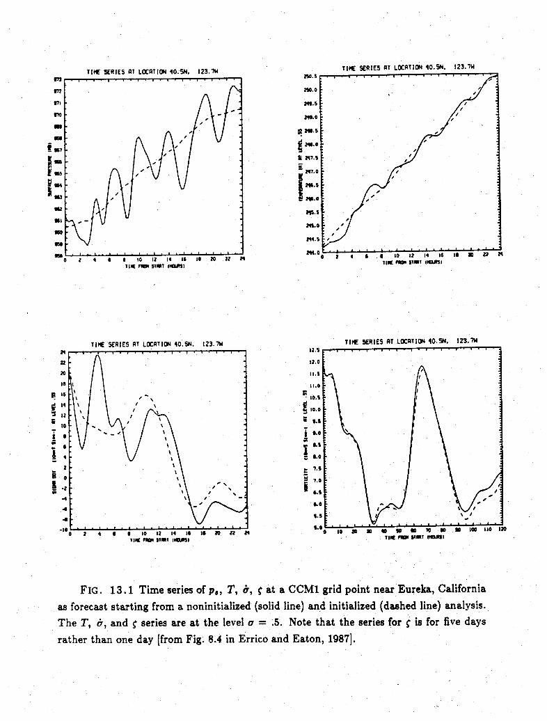
TIME SERIES AT LOCATION 40.5N. 123.7W

list n STaT IESMI

TIME SERIES AT LOCATION 40.SN. 123.7W

3

IIsIIv.

I

I

TIME SERIES AT LOCATION 40.5N. 123.7W

TIli rio SlTT (IOSI

FIG. 13.1 Time series of p., T, 6, q at a CCM1 grid point near Eureka, California

as forecast starting from a noninitialized (solid line) and initialized (dashed line) analysis.

The T, o6, and ' series are at the level a = .5. Note that the series for ~ is for five days

rather than one day [from Fig. 8.4 in Errico and Eaton, 1987].

TIMESERIS A LOCTIO 40.N, 23.7W

i

I

tr

!

Briere, 1982; Du Vachat, 1986). In the latter models, effects of the boundaries must

be considered since the fields are not generally periodic within the regional domains. In

some limited-area schemes, boundary effects are simply considered as a type of "forcing"

similar to the nonlinear terms, and the modes themselves are considered periodic. For

some regional models, another complication is created because the grid coordinate system

renders the linear operator £ nonseparable in the two horizontal directions if either map

scales or variations of f are considered in the linear problem. In this case, either further

approximation is required (such as ignoring map-scale factors and variations in f) or a

large numerical eigenvalue problem must be considered.

14. Implicit NNMI

Implicit NNMI schemes (Temperton, 1988; Bourke and McGregor, 1983) are equiv-

alent to explicit NNMI schemes, except they are formulated in terms of b, 6, and <p on

the model's horizontal grid rather than in terms of normal mode coefficients. Balance is

expressed in terms of the vertical-mode equivalent of (10.12-14); e.g., as

foe - V2 Pt + N6e = 0, (14.1)

-[fo2 gHetV 2] tc + foNte - V 2N, = 0, (14.2)

Ptg- fork , (14.3)

where the last is intended to express the constraint that P is not to be altered by the

initialization. For the modes defined in Part II, this constraint is equivalent to unalteration

of the rotational mode amplitudes r in Machenhauer's (1977) explicit NNMI, since r is

proportional to P at each 3-dimensional scale. For other linearizations or definitions of P,

the constraints may not be equivalent although they may be quite similar. In particular, for

modes defined on the sphere, (14.3) with fo replaced by f is not equivalent to unalteration

of the rotational modes.

Equation (14.1) may be combined with (14.3) to yield

[fo2 - gHeV 2] lt + foNse + gHtV 2 P = 0 (14.4)

73

which may replace (14.1). Note that the linear operator fo - gHeV 2 now appears in

both (14.2) and (14.4). Solutions of (14.2-4) for ¢ and S are used to determine p and ;A,

respectively, as solutions to the Poisson equations

V 2' = st, (14.5)

V 2 it = At, (14.6)

using some appropriate, model-dependent, boundary conditions. From ' and x, u and v

are determined as

ut= Xe a- ' (14.7)

Oxt OytvI= X + -'P' (14.8)

Solutions for p are used to determine both T and p., as described in Section 11.

Generally, (14.2-4) are iterated in a form analogous to (13.1-2); e.g., as

[fIo - gHeV2 ] AI = -fo o (14.9)

[fo - gHeV2 ] A = f to V2 , (14.10)

, = gHtfo-f 1^i, (14.11)

where

iS+ 1' =: S + 'Ao , (14.12)

[+1 = 6 + A\ t (14.13)

t:+ 1 = + AZ t, (14.14)

I is an iteration counter, and the tendencies are computed from values of the fields

determined for the superscripted iteration; i.e., the right hand sides of (14.9-10) are

determined by the fields u1, v 1, T', and pi. The constraint on P is explicitly expressed as

(14.11), but also appears implicitly in (14.9).

74

The first iteration (I = 0) may be determined by either a noninitialized analysis or a

linearly-initialized analysis. The latter is the solution to

fo = V2t, (14.15)

6 = 0, (14.16)

(f 2 - gHtV2 ) te = -fogHtPet (14.17)

These equations are simply the geostrophic balance equations expressed for an f-plane,

where both t and p are to be determined by P. The latter condition contrasts with

most past applications of geostrophic balance which more typically constrain either ' or

p. Other constraints than the one in terms of P may be used, but this one is equivalent to

the constraint that the linear initialization does not alter the rotational mode coefficients.

With the latter constraint, a subsequent forecast is unaltered to the extent that it depends

on the rotational mode coefficient specification only (Daley, 1981b). Also, it is possible to

formulate these expressions for variable f (see Temperton, 1988)

An obvious advantage to implicit schemes is that the 3-dimensional eigenvectors do

not need to be determined. Only the vertical modes need to be explicitly calculated.

Additionally, their implementation on the model's grid facilitates any modification to the

NNMI scheme to include, for example, a variational analysis (Temperton, 1988; Fillion and

Temperton, 1989). A disadvantage to the implicit schemes is that horizontal-scale or mode

selectivity is not as straightforward as for explicit schemes (since the latter are explicitly

formulated in terms of scales). Also, if a diagnostic analysis is to be performed (e.g., the

analysis of balance described by Errico, 1989c), then the determination of normal modes

is useful for diagnostic purposes in addition for use by the NNMI scheme.

A result of implicit NNMI applied to a limited-area forecast model is presented in

Fig. 14.1 where several time series in forecasts begun from analyzed fields with and without

NNMI (respectively indicated by dashed and solid lines) are shown for selected fields at

one point in the model. This example is taken from Errico and Bates (1988), where the

PSU/NCAR MM4 was used starting from an enhanced NMC analysis for OZ 22 April 1981,

75

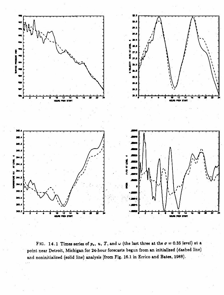
40 1

II

$on MM VWT I M

Am

-AM

- 1 2 4 · 1 12 14 13 l 3 2

FIG. 14.1 Times series of pe, u, T, and w (the last three at the a = 0.35 level) at a

point near Detroit, Michigan for 24-hour forecasts begun from an initialized (dashed line)

and noninitialized (solid line) analysis [from Fig. 16.1 in Errico and Bates, 1988).

I

3.4

MS.2

qv 3M.9

34.6Md.@

X3.4

)a.6

X1.4

3-.2

/

II

/I

/

p . p * p * p * p * p * p. p * p * p *

........ i

and the NNMI scheme was applied to the three largest vertical scales only. Note in the

figure that "noise" has been reduced by NNMI in the fields of p., T, u, and w, although

values of those fields at hour 24 do not appear significantly affected by the initialization.

Results for other model points appear qualitatively similar, indicating that the NNMI

procedure has successfully reduced gravitational noise without significantly affecting slower

components of the fields during the 24 hour forecast. The oscillations still present in the

forecast time series may be due to quasi-geostrophic dynamics, or to propagating internal

gravitational waves at vertical scales which the NNMI has ignored, or to a noise generation

effect of the lateral boundaries.

15. Further Considerations

NNMI is a fairly straightforward method to apply to most numerical models. 'How-

ever, there are several important details regarding its application which are not yet well

understood. Furthermore, many misconceptions exist regarding what NNMI is actually

designed to do. Several of these details are addressed in this section.

15.1 NNMI vs. no NNMI

Most properly, the NNMI balance condition should be considered as another piece of

information to be considered in producing an initial state; i.e., as part of the analysis.

However, NNMI is typically applied only after an analysis has been performed. That

analysis generally attempts to produce an optimal estimate of the fields as defined in some

statistical sence, but a subsequent initialization likely renders the final initialized analysis

less than optimal. Surely, if the fields are truely balanced in the atmosphere according to

the NMMI conditions, then the analysis itself should reflect that. The consideration of

NNMI as part of the analysis itself has been discussed by Daley (1980), Tribbia (1982),

Barker (1982), Williamson and Daley (1983), Lorenc (1986), and Fillion and Temperton

(1989).

77

A consequence of the analysis ignoring NNMI is that the analysis is less than optimal

in the context of a data assimilation system. If the initialization is performed only after

the analysis is produced, then the initialization will immediately affect only gravitational

modes. Presumably, those modes would adjust during the subsequent forecast if no NNMI

were performed. Typically their affect on forecasts is limited (except for the presence of

noise, which can be removed by some other process, such as finalization; cf., Williamson

and Temperton, 1981), even though the changes produced by the initialization may be

large in some locations (e.g., in pressure troughs or near steep mountains). A greater

and more immediate effect on the forecast may be realized if it is recognized that the

modes unaffected by the NNMI may be in error, yielding imbalances through errors in the

nonlinear terms. This last effect suggests that other modes (such as the rotational modes

or corresponding fields of potential vorticity) also should be altered in order to achieve

the most realistic balance (i.e., that balance most consistent with the observations and

background data). For further discussion of these points, the reader should consult one or

several of the papers mentioned above.

It should be emphasized that in many cases, NNMI has no significant impact on the

forecast directly. In other words, those components responsible for the gravitational noise

may have no significant impact on the complementary components which describe the

important cyclones and anticyclones responsible for our weather (e.g., see Daley, 1981b).

Apparently the former components propagate too fast and are too weak to impact the

latter. An exception to this noninteraction likely occurs in cases where gravity waves

excite instabilities, such as convective instabilites (again, see Daley, 1981b), however it

is not clear that those modes normally initialized even have much impact on convection

(since NNMI is usually restricted to modes of large equivalent depth). Instead, the biggest

impact of initialization has generally been the removal of noise from background (i.e., first-

guess) fields used during an analysis-initialization-forecast cycle, as discussed in Part I. In

other words, even if it is not part of an optimal analysis scheme, NNMI still impacts the

78

analysis through providing a better, relatively noise-free background field for the analysis

scheme to use as a first guess.

The aboved mentioned results regarding the impacts of initialization also explain

some common misconceptions concerning the application of NNMI. Typically, a forecast

of synoptic fields produced from an analysis which has been subsequently initialized will

not be more accurate than one begun from the corresponding analysis alone, once the noise

has abated. The NNMI removes noise, as it has been designed to do, with minimal affect on

the remaining components of the forecast. It is only when coupled with an analysis system

that the final forecast itself is improved (unless the measure of skill actaully emphasizes

components described by fast gravitational modes).

It should also be mentioned that there are other methods which can be applied to

reduce gravitational noise in numerical forecasts. Those methods primarily are various

types of temporal filters applied as part of the model's time integration scheme or spatial

filters applied to gravitational-mode related fields, such as wind divergence (see e.g.,

Haltiner and Williams, 1980). Those methods may be successful although they may

have two significant drawbacks: they take time to affect an adjustment during a forecast;

and they may affect the character of the balance toward which the model adjusts. This

latter effect occurs if either a mode's frequency or the "nonlinear" term which forces

it is altered by the filter, either implicitly or explicitly. For example, adding strong

diffusion to the divergence field generally acts to add another term to the balance equation

satisfied by the model, thereby altering the adjusted solution in addition to dissipating the

propagating gravity wave components. Filtering methods can be used with care, although

it is unapparent how they are more appropriate than NNMI schemes.

15.2 Selection of modes to initialize

An important question to answer before performing an initialization is: Which modes

are to be initialized? If an implicit NNMI scheme is to be used, the corresponding question

79

is: To which vertical and horizontal scales should the initialization be applied? These

questions actually have many diverse aspects which each require investigation. For this

reason and the fact that some aspects are currently (almost) impossible to investigate,

these questions have not been answered completely, although several papers have addressed

them (e.g.: Errico, 1983, 1984b, 1989a, 1989b, 1989c; Errico and Rasch, 1988; Errico and

Williamson, 1988; Errico et al., 1988; Puri, 1983; Puri and Bourke, 1982).

In order to determine which modes should be initialized, it is important to consider

the following questions:

1. To what degree is each mode or scale balanced in the atmosphere? We would

like the initialized analysis to reflect the real atmosphere.

2. To what degree does each mode or scale in the model tend to a nonlinear

adjusted state? The model forecast will tend to adjust to its own balance,

whether or not it is the same as that of the atmosphere.

3. What problems are caused by not initializing certain scales or modes? If

initialization has insignificant impact on the forecast or on other uses of the

analysis, it is unnecessary.

4. What are the magnitudes of the analysis errors compared to the adjustments

produced by the initialization? Clearly if the adjustments are within the noise

range of the analysis errors, the initialization cannot be considered a disruption

of the analysis.

Currently, the first and last questions are extremely difficult to answer since the

atmosphere is not observed sufficently well. In particular, the atmospheric fields (e.g.,

horizontal velocity divergence) which project onto gravitational modes are not observed

adequately (otherwise, initialization would likely be unnecessary). Even estimates of the

analysis errors are difficult to determine, since there is little independent data with which

80

to compare. This last problem is discussed further in Daley and Mayer (1986) and Tribbia

and Baumhefner (1988).

One way of estimating answers to the first question is to use a simulation model to

mimic the atmosphere. This is discussed further in Part V. Examination of the behavior of

the simulation model also suffices to answer question 2. This is likely the simplest question

to answer since the model equations, physics, and fields are all known precisely.

The third question has some difficult aspects to consider. We must attempt to

distinguish problems caused by analysis errors, initialization errors, and model (physics

or numerical) errors. These errors all interact in complex ways, so it can be misleading to

characterize the result of a poor forecast as due to the the selection of modes initialized.

It is also important to note here that the problem can be easily misinterpreted as due to

the selection of modes when it is more properly attributable to other details of the specific

NNMI method used (e.g., the iteration scheme itself).

Since only a few aspects of these four questions have been investigated as of yet, it

is impossible to state any definitive answer to the question of which modes to initialize.

However, some comments taken from the references cited above are in order:

1. Fast, large depth modes appear to be well balanced in model simulations for

straightforward theoretical reasons which presumably apply equally well to the

atmosphere;

2. The above set of modes particularly includes all the external gravitational

modes;

3. There is theoretical and observational evidence which strongly suggests that

slow, internal tropical modes (such as Kelvin modes) are not balanced in either

the atmosphere or simulations.

4. If no initialization is performed, the model will adjust toward a balanced state in

any case, and the forecast will eventually appear similar to a properly initialized

81

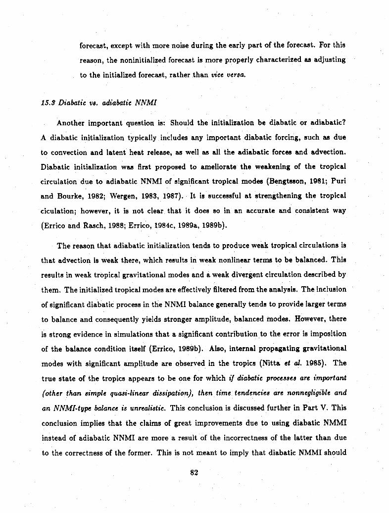
forecast, except with more noise during the early part of the forecast. For this

reason, the noninitialized forecast is more properly characterized as adjusting

to the initialized forecast, rather than vice versa.

15.S Diabatic vs. adiabatic NNMI

Another important question is: Should the initialization be diabatic or adiabatic?

A diabatic initialization typically includes any important diabatic forcing, such as due

to convection and latent heat release, as well as all the adiabatic forces and advection.

Diabatic initialization was first proposed to ameliorate the weakening of the tropical

circulation due to adiabatic NNMI of significant tropical modes (Bengtsson, 1981; Puri

and Bourke, 1982; Wergen, 1983, 1987). It is successful at strengthening the tropical

ciculation; however, it is not clear that it does so in an accurate and consistent way

(Errico and Rasch, 1988; Errico, 1984c, 1989a, 1989b).

The reason that adiabatic initialization tends to produce weak tropical circulations is

that advection is weak there, which results in weak nonlinear terms to be balanced. This

results in weak tropical gravitational modes and a weak divergent circulation described by

them. The initialized tropical modes are effectively filtered from the analysis. The inclusion

of significant diabatic process in the NNMI balance generally tends to provide larger terms

to balance and consequently yields stronger amplitude, balanced modes. However, there

is strong evidence in simulations that a significant contribution to the error is imposition

of the balance condition itself (Errico, 1989b). Also, internal propagating gravitational

modes with significant amplitude are observed in the tropics (Nitta et al. 1985). The

true state of the tropics appears to be one for which if diabatic processes are important

(other than simple quasi-linear dissipation), then time tendencies are nonnegligible and

an NNMI-type balance is unrealistic. This conclusion is discussed further in Part V. This

conclusion implies that the claims of great improvements due to using diabatic NMMI

instead of adiabatic NNMI are more a result of the incorrectness of the latter than due

to the correctness of the former. This is not meant to imply that diabatic NMMI should

82

not be performed, since its use as a "fix" may be appropriate. However, it does imply

that "better" specification of the diabatic forcing will not yield a better initialized analysis

unless the NNMI balance condition is significantly altered.

15.4 Choice of starting iterates

In the past, there had been some debate as to what the proper starting iterate should

be for use in an NNMI scheme (Phillips, 1981). There is evidence that in some contexts the

resulting solutions to Machenhauer's scheme are not very sensitive to the starting iterate

(Errico, 1983; also see Section 13). However, if the scheme is restricted to only a few

iterations, the choice of a starting iterate may be important.

If a linear initialization is used as a starting iterate, then all information in the analysis

which directly describes the modes to be initialized is discarded. The only information

regarding the discarded modes is provided by the balance condition and other modes.

Some information can be regained by sufficiently iterating the NNMI condition, at least

for those modes to which the NNMI balance condition properly applies (such as external

gravitational modes). However, there is no reason to generally remove such information

from the starting iterate. Motivations based soley on results of single-parameter scalings

(such as application of the scheme of Baer and .Tribbia, 1977) are insufficient for discarding

such information (see Section 13 and Part V for further discussion).

15.5 Consequences of incorrect mode determination

As a final question of this section, it is relevant to ask: What are the consequences

of improperly defining the model or atmospheric modes due to improper linearization?

An improper linearization includes both neglect of terms in the linearization process and

neglect of the true atmospheric state in defining the basic state. An example of the former

is neglect of consideration of the model time scheme or diabatic terms, and an example of

the latter is defining the basic state as one with zero wind.

83

There are two effects to consider. One is the effect on the fields produced as a result of

NNMI. The other is the effect on using normal modes as an analysis tool, which is related

to the results of a linear initialization.

In NNMI, an equation of the form

g = -N(r,g) (15.1)

is solved for g where r represents the constrained components (such as the rotational modes

or linearized potential vorticity). One result of an improper linearization is a replacement

of 4g by

£'g = £g- Ag . (15.2)

The nonlinear term which is defined as "everything not linear" is thereby also changed

such that the new term is

N N + ACg. (15.3)

The equation corresponding to (15.1) for the new linearization is

-'g7= -N'(r,g) (15.4)

which by substitution of (15.2-3) is equivalent to (15.1) and thereby yields the same solution

for g. Of course, it may be that the method used to solve (15.1) may be satisfactory, but

fail for (15.4). However, if true unique solutions are found, they will be identical for both

equations. Essentially, moving a term or portion of a term from one side of the balance

equation to the other does not change the balance, or equivalently, calling one term or

portion of a term "linear" and the remainder "nonlinear" does not alter the condition

dg/dt = O.

Notwithstanding the former claim, there is an effect of altering the linearization,

besides simply relabeling terms as either "linear" or "nonlinear". That effect is to alter

the constraints on the solution. In other words, changing the definition of the modes (which

84

is an effect of changing the linearization) changes what we distinguish as the atmospheric

components to be altered. Some portion of what we called "rotational modes" modes in

one case may now be relabeled as "gravitational modes". Such a change will alter the

solution to (15.1), although the change may be small if the relabeling is not significant.

An example of this effect is presented in Errico (1984a). We reiterate by stating that the

stationary solutions to (3.3-11) are not dependent on any linearization, and therefore the

solutions to a nonlinear balancing of all the dynamic fields are also independent of anylinearization; the effect of the linearization in NNMI is instead to distinguish components

to be initialized from those to be constrained.

Of course, the results regarding a linear initialization may be much more significantly

dependent on the linearization, because the linearization defines which modes are removed

and the compensation due to (15.1-4) does not apply. Therefore, it behooves the user tochoose an appropriate linearization if his intent is to analyze dynamic fields into normal

mode components. For example, using a basic state with zero wind may be inadequate for

analyzing Rossby waves on the sphere, because the Rossby modes so determined are allassociated with frequencies corresponding to westward propagation, rather than eastward

as observed in an atmospheric or nonlinear context. The inappropriate specification oftheir frequencies implies that their individual structures may also be defined anappro-priately, since each are determined by corresponding eigenvalues and eigenvectors, whichare themselves intimately related. Whether or not this specification of Rossby waves is

appropriate clearly depends on the intended use of the mode definitions. The choice of abasic state is also discussed in Section 3.

85

PART V. NNMI AND QUASI-GEOSTROPHIC THEORY

In Section 10 the relationship between the quasi-geostrophic equations and the NNMI

balance condition was discussed. Here, we discuss the fundamental question: Why is

the extratropical atmosphere quasi-geostrophic. First, it will be demonstrated that some

common answers to this question are incomplete or incorrect. Then a more complete

answer will be given essentially following the arguments of Charney (1955, 1973). Some

of the limitations of quasi-geostrophic theory will be highlighted along the way, especially

regarding small vertical scales.

The scale analysis of Section 7 will be repeated in Section 16 with the constraint on

the time scale relaxed in order to demonstrate that the question we ask actually regards

the determination of the observed time scale. In Section 17 very detailed scale analyses

are presented in terms of both vertical and horizontal scales using results produced by

simulation models. This is followed in Section 18 by a description of gravity wave behavior

in a global simulation model, where the appropriateness of the prognostic normal-mode

equations is demonstrated (at least for some scales) and the time scales of individual modes

are examined. Finally in Section 19 the characteristics of atmospheric forcing, stability,

and dissipation are discussed regarding how they act together to produce predominately

slow temporal variations of the dynamic fields (i.e., how they produce something which

appears as a slow manifold).

16. Scale Analysis in Terms of a Rossby Number

A correct scale analysis for the whole range of behaviors describable by the prim-

itive equations requires consideration of many scales; i.e., both spatial and temporal

spectra. However, such a scale analysis necessitates the simultaneous use of several scaling

parameters and the consideration of details of the scale interactions (which are nonlinear).

86

Consequently, such an analysis has many degrees of freedom and yields highly complex

nonlinear equations. An analysis of this complexity will be performed as a diagnostic

calculation in Section 17, but here only a single-parameter scaling will be considered. This

will be a scaling in terms of a Rossby number. In this regard it is similar to the analysis inSection 7, except here no attempt will be made to predispose the result to quasi-geostrophic

conditions.

For a simple scale analysis, it is most appropriate to consider the primitive equations

m the form of systems of shallow water equations expressed in terms of /f and S/fo which

may be derived from (4.12-4.14) with reconsideration of the nonlinear terms. This form

is appropriate since the vertical scales are explicit in terms of the equivalent depths, and

different scaling for the rotational and divergent wind fields may be easily and explicitly

considered. The equations may be written as

6 1 , (61 A

fTdtf 0 - +T +T2N' (16J )1o 96 f< f H 0 £

1 C1 b g HV2 V +-2N 6 (16.2)fo t fo f H fo 2

fo cOt gH = ~ff~~~dtgH ~~~+ gn fo 1 (16.3)

where division by factors of fo and gH have been applied to render all terms dimensionless

and to facilitate subsequent scaling.

As is typical, our Rossby number will be defined as

£ = U/foL, (16.4)

where U and L define velocity and length scales, respectively. This definition is not

Rossby's original definition, which was as the ratio of the inertial time scale (equal to

fof 1) to the observed time scale. Instead, we will denote the inverse of the observed time

scale as fl and use it for the scaling of 9/8t. Definition 16.4 is equivalent to Rossby's

definition only when 01 is given by the inverse of the advective time scale (i.e., when

11 = U/L) as was assumed in Section 7. Our Rossby number will be used to scale the

87

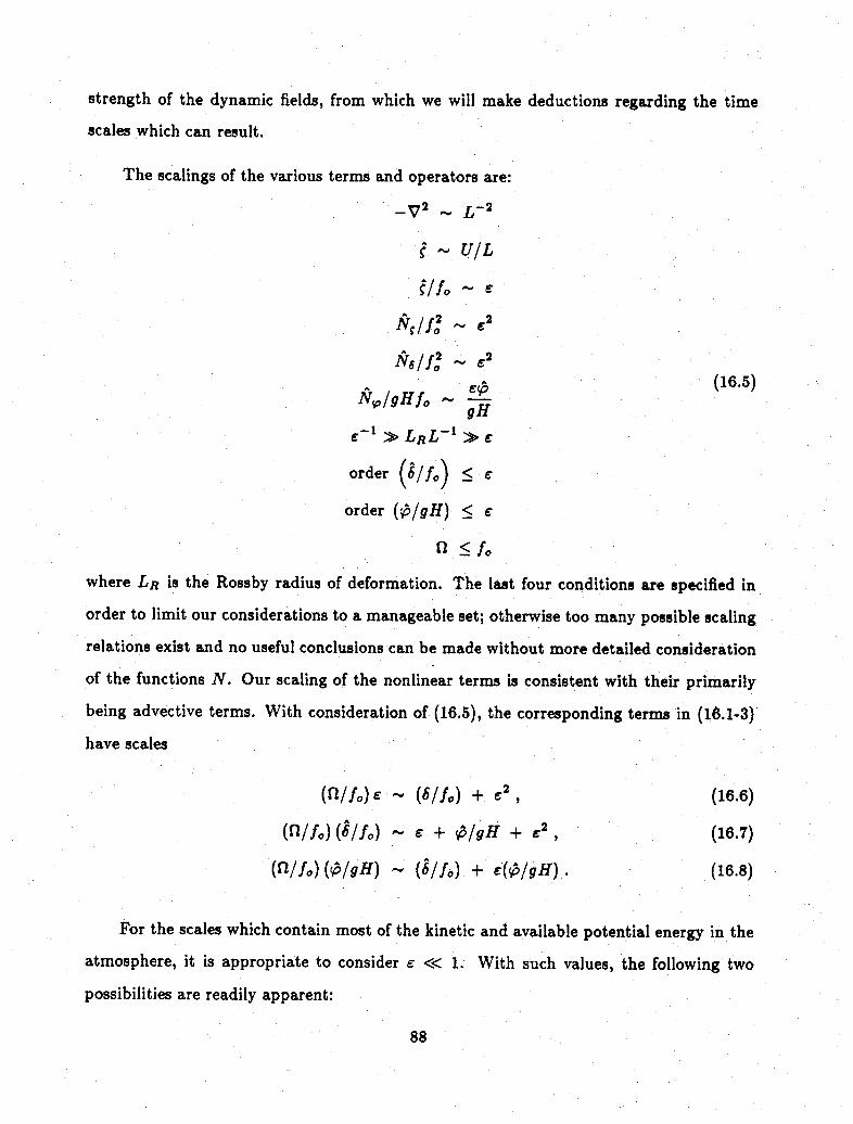
strength of the dynamic fields, from which we will make deductions regarding the time

scales which can result.

The scalings of the various terms and operators are:

-V 2 ~ L-2

- U/L

/fo ( 2

N6/ fo ~ e

(2jO (16.5)NI/gHfo

gHc - 1 > LRL -1 c

order (6/fo) < c

order (/g9H) < €

n _fo

where LR is the Rossby radius of deformation. The last four conditions are specified in

order to limit our considerations to a manageable set; otherwise too many possible scaling

relations exist and no useful conclusions can be made without more detailed consideration

of the functions N. Our scaling of the nonlinear terms is consistent with their primarily

being advective terms. With consideration of (16.5), the corresponding terms in (16.1-3)

have scales

(nlfo) E (6/fo) + 2, (16.6)

(fl/o) (6/fo) + I/gH + c2, (16.7)

(n/fo) (P/gH) (6/fo) + €({/gH). (16.8)

For the scales which contain most of the kinetic and available potential energy in the

atmosphere, it is appropriate to consider e<< 1. With such values, the following two

possibilities are readily apparent:

88

(1) The dynamic behavior is characterized by the inertial time scale (I ~ fo) implying

P/gH E~ , 6/fo ~ F, and C6/f/2t ~ E. These first order solutions are inertial

gravitational waves.

(2) The dynamics are characterized by the advective time scale (fl/fo ~ ) implying

I/gH E~ , 6/fO c2, and c6/fo2t 3. These first order solutions are geostrophic,

and the second order solutions are quasi-geostrophic, as discussed in Section 7.

The important point in the above analysis is that even if the Rossby number definedas U/foL is small, gravitational waves may still be first-order solutions. It is only whenthe additional assumption or condition that the time scale is advective (and not inertial)

is imposed that this simple Rossby number scaling argument results in a conclusion thatsmall E implies quasi-geostrophy. Of course, by saying that the time scale is longer than

inertial already omits the possibility of significant amplitude (i.e., first-order) gravity waves

since they have inertial time scales, which is a fact omitted in most texts. Therefore, the

key question of why the atmosphere is quasi-geostrophic may be restated as the question:Why is the observed time scale advective rather than inertial? The answer to this question

requires further consideration of the dynamics and not just a simple one-parameter scalingargument. The answer will be discussed in Section 19.

17. Scale Analysis of Nonlinear, Diabatic Model Simulations

Thus far, the scale analysis of Sections 7 and 16 have been in terms of a single,Rossby number parameter. These scalings yield correct asymptotic results; i.e., as c -_ 0.However, an appropriate value of c for the atmosphere is likely not significantly less than

0.1, which is not a very small number when considering all the other factors abounding inthe equations (e.g., it takes only a few terms of order 0.01 to sum to a term not significantly

less than 0.1). Also, the atmosphere and models include many horizontal and vertical scales

89

simultaneously, and permit complex interactions among them. Therefore, it is appropriate

to perform a more detailed scale analysis by explicit consideration of spatial spectra.

For this purpose, we will consider the prognostic equation for a generic mode coefficient

Cj to have the form

dc = -iAc + Aj + Dj , (17.1)

where A represents all the nonlinear adiabatic terms, which may be expressed as

A = N(r) + N(rg) + N(g), (17.2)

and D represents all the adiabatic terms. The N here are different functions of different

variables, considered to be at least quadratic in the indicated variables: the r signifiesthat N(r) depends only on rotational mode coefficients; the g signifies that N(g) depends

only on gravitational mode coefficients; and the rg signifies that N(rg) depends only on

products of rotational and gravitational mode coefficients with each other.

One way of scaling the terms in (17.1) for various sets of modes would be to determine

them directly from analyzed atmospheric data. However, such analysis are not sufficiently

accurate to correctly describe gravity wave behavior at most scales. The analysis may

provide bounds on the magnitudes of various terms, or may provide good estimates at

some locations; however, global analyses of small terms is not possible.

Fortunately, simulation models appear to be very useful for performing detailed scale

analyses. All terms can be accurately determined in the context of model data as long

as the computer has sufficent precision. A model is necessary in any case because some

mathematical forms of the atmospheric forces are necessary. In a model, those forms and

the simulation are self consistent. Of course, results of the simulation may be differentfrom those of the atmosphere. Care must be taken in drawing and applying conclusions

derived from simulations. However, if results can be explained in terms of processes or

relationships known to exist in the atmosphere, and if qualitatively similar results are

obtained with significantly different models, then we will have more confidence in the

general applicability of our results.

90

Even if a forecast model gives significantly unrealistic results regarding atmosphericbalance, it is important to investigate the balance toward which it adjusts. We obtain usefulinformation regarding errors in its formulation of dynamics or physical processes. Also,since the model will adjust to its own balance anyway, it may be appropriate to initializeit to that balance since unrealistic gravity waves would otherwise be created; i.e., it isthe difference between its own balance and its initial analysis which determines its initialgravity wave noise, not the difference between the initial analysis and the correspondingreal atmospheric balance.

17.1 Global model results

Model generated balances of global NWP models have been reported by Errico (1984b)and Errico, Barker and Gelaro (1988). Both studies used different models. The main pointof the second study was to demonstrate the generality of the first study and to extend itto higher resolution. The first study has more details regarding the generated balance, butin this section results from the second study will be described. This study will be denotedby the initials EBG.

EBG used two U. S. Navy operational global NWP models. Since in most importantrespects, results from both models were qualitatively identical, results for only their secondmodel will be discussed here. That model was a 15 level spectral transform model truncated

at triangular 47. It included parameterizations for convection, radiation, and boundarylayer dynamics. Its horizontal transform grid included 72 latitudes and 144 longitudes.

EBG made a 20-day forecast beginning from an operationally produced analysis, withno NNMI. Each term in (17.1) was evaluated for each mode by post processing the forecast.They were evaluated for instantaneous times (i.e., no time averaging was performed) nearthe end of the forecast, so that nonlinear geostrophic adjustment had presumably occurred.

91

Results were presented in terms of graphs of normalized and averaged squared moduli

(i.e., sums of squares of real and imaginary parts) of terms. All terms were presented

in single figures, with distinct figures for distinct equivalent depths. Only gravitational

modes were considered (but see Errico, 1984, for presentation of rotational modes). The

normalization and averaging was performed by considering 40 contiguous ranges of A for

each equivalent depth. The squared moduli of all modes whose A fell within a single range

were summed together before taking the square root. Normalization was accomplished

by dividing the rms moduli of the terms within each range by the similarly computed

rms moduli of the coefficients themselves within that range. The ranges were chosen such

that 28 modes were included in each range, except for the highest-frequency range which

had 36 modes. The intention of the averaging was to produce representative values for

similar horizontal and vertical scales (since A is scale dependent), and the normalization

was intended to reduce the range of the ordinate on the figures. For example, one effect of

the normalization was to make the normalized rms values of iAc approximately equal to IA[,

but without normalization the spectrum of these rms values would have been dominated

by magnitudes of Icl instead.

Within each range, the normalization factor was identical for all terms, so that the

rms magnitudes of terms relative to each other were preserved. Therefore, modes within a

range were considered characterized by balance if the normalized rms tendency term was

significantly smaller than some other term. Where balance existed, the largest terms were

typically the linear and nonlinear adiabatic terms. Obviously, since these must sum to

yield a much smaller tendency, the terms must generally have opposite signs, implying an

adiabatic nonlinear balance (although the sense of the signs is lost in the presentation of rms

values in the figures). Individual modes were also examined (i.e., without range averaging)

to insure that the relative rms magnitudes were actually representative of individual modes

rather than artifacts of the averaging process.

92

Figures 4-6 from EBG are reproduced here as Figures 17.1a-c. The tendency, linear,

and adiabatic terms are labeled as E, A, and B, respectively. The diabatic term is

divided into contributions by latent and radiative heating (label C) and eddy-diffusive and

boundary-layer processes (label D). The three figures correspond to the modes t = 1,5,15

with respective equivalent depths 10 km, 137 m, and 0.36 m. Abscissas are labeled by an

w for each frequency range, defined as the geometric mean value of the A for modes within

that range. Larger w correspond to smaller horizontal scales (as suggested by equation

4.33).

The fact that, for any w in Figure 17.1a, values of curve A are 10 or more times

corresponding values on curve E indicates that the linear term is at least an order of

magnitude larger than the time tendency for external gravitational modes of all resolved

horizontal scales. For this to be so, the linear term must be approximately balanced. Here,

since curves B and A are similar, that balance is a nonlinear adiabatic one, corresponding

to Machenhauer's (1977) condition (our equation 9.1). For these modes, diabatic processes

are weak, as indicated by the relatively small values of curves D and C.

For the e = 5 modes in Figure 17.1b, the linear term is again shown to be larger than

the tendency term at all horizontal scales, however, rather than 10 times larger, that factor

is 2 or less. In other words, there is not as strong a degree of balance as for the external

modes. Note that the balance is again adiabatic.

For the t = 15 modes in Figure 17.1c, there is no indication of balance since the

tendency term appears as large as the linear or nonlinear term at almost all horizontal

scales. Boundary layer and diffusive processes are also strong for these modes.

The results from EBG are similar to the results of Errico (1984b) in many respects.

In particular, relatively high-frequency gravitational modes, such as the external ones,

appear to be strongly balanced in the realistic global models. Shallower modes, which are

associated with lower frequencies, are generally not as well balanced, if at all. Also, usually

at the scales where balance exists, that balance is adiabatic. If diabatic processes are a

93

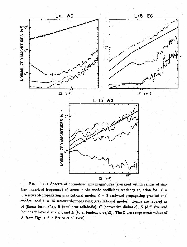
L=l WG

II-4

L=5 EG

(s-')

I

0

z

o

0LJN

(T0z

L=15 WG

(s-')FIG. 17.1 Spectra of normalized rms magnitudes (averaged within ranges of sim-

ilar linearized frequency) of terms in the mode coefficient tendency equation for: e =

1 westward-propagating gravitational modes; t = 5 eastward-propagating gravitational

modes; and t = 15 westward-propagating gravitational modes. Terms are labeled as

A (linear term, iAc), B (nonlinear adiabatic), C (convective diabatic), D (diffusive andboundary layer diabatic), and E (total tendency, dc/dt). The W are range-mean values of

A [from Figs. 4-6 in Errico et al. 1988).

I

significant part of the balance, as at some scales in Errico (1984b), then those processes

typically are quasi-linear surface drag or diffusive processes, not convective or radiative

processes.

An additional result in Errico (1984b) is a determination of the ordering of terms in

(17.2). For the external rotational mode tendencies, time-mean magnitudes of N(r), N(rg)

and N(g) typically have the ratios 15:2.5:1 while for external gravitational modes, the

ratios are 20:2:1. Although the ordering from largest to smallest magnitude is anticipated

by ther relation » g, the specific factors cannot be anticipated by a single-parameter

scaling. Typical ly for the external gravitational modes, N(rg) 2 dg/dt, which indicates

that the N(rg) term does participate in a balance condition. This term is included in

Machenhauer's (1977) balance condition , but is excluded from the lowest-order nonlinear

balance defined by Baer and Tribbia (1977). Its exclusion results from the ordering of both

N(rg) and dg/dt as e3 terms (Section 7). For much shallower modes, N(r) N(rg) which

is another result not revealed by a Rossby number scaling.

17.2 Mesoscale model results

An analysis similar to that of EBG was applied to a regional, mesoscale model by

Errico (1989c). That model was the PSU/NCAR MM4, discussed in Sections 12 and 14.

His intention was to investigate possible balances on horizontal scales much shorter than

in the context of EBG. The MM4 was therefore used with a grid spacing of 50 km. Its

domain covered the contiguous United States. Four-day forecasts were produced from

interpolated, initialized FGGE analysis, but the analyses were not reinitialized to make

them consistent with the MM4 formulation or resolution.

Model forecasts were analyzed at 24 hour intervals. Vorticity, divergence, and pseudo-

geopotential were determined and projected onto the model's vertical modes. Forces were

determined using a method similar to EBG. Horizontal scales were determined by two-

dimensional Fourier analysis of detrended fields using the method-of Errico (1985). Normal

95

modes (other than their vertical components) were not determined. Results were presented

as functions of horizontal and vertical scales of terms in either the prognostic divergence

or ageostrophic equations, respectively considered as

86^ ^~~~a+A6s~~~+D6~ ,(17.3)at = + A + D,

atat=- ( -rV 2 ) 6+Aa+ a, (17.4)

where a = ff - V 2 ,p A and D distinguish the adiabatic and diabatic components of N,

and Na = foNC - V 2N,. These equations are those presented as (10.12-10.13), except

with reconsideration of the tendency terms and the change in notation. Presented values

were normalized analogously to EBG.

Here, only terms in the ageostophic tendency equation for Errico's (1989c) winter

case will be reproduced. Terms for the t = 1,4,10 modes appear in Figures 17.2a-c and

17.3a-c for the 6 and a equations, respectively. The tendency, linear, adiabatic nonlinear,

and diabatic terms are labeled as T, L, A, and D, respectively. Note that the ratio

L/T is approximately 200, 5, and 1 for t = 1,4, and 10, respectively, at most horizontal

scales. At scales where balance exists, it is approximately adiabatic (i.e., L t A >> D),

except at the smallest horizontal scales where parameterized eddy diffusion is important.

Similar qualitative results apply at all forecast times beyond hour 36 and for other synoptic

situations, including summer simulations.

The results of Errico (1989c) highlight the strong dependence of model generated

balance on vertical scale. Large vertical scales generally tend to be balanced and small

vertical scales unbalanced, with the imbalances defined by nonnegligible magnitudes of

observed tendencies. One important implication is that NNMI-type balance conditions

appear to be appropriate only for large equivalent depths. Another implication is that

appropriateness of either nonlinear balance equations (Charney, 1955) or quasi-geostrophic

omega-equations (Phillips, 1960) for initialization or diagnostic description of the atmo-

sphere is similarly restricted to large vertical scales. In particular, the use of a quasi-

96

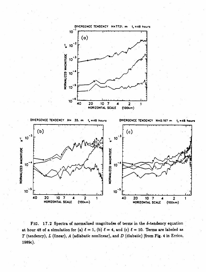
10

| 10

I-= 10

z

42

0

2

0K

o 10

DIVERGENCE TENDENCY H=7721. m s 48 hours-1

-4

' 40

DIVERGENCE TENDENCY H= 35. m

40 20 10 7 4 2HORIZONTAL SCALE (100km)

20 10 7 4 2 1HORIZONTAL SCALE (100km)

t, =48 hours

1

DIVERGENCE TENDENCY H=0.167 m t =48 hours

I

0

i

oz

40 20 10 7 4 2HORIZONTAL SCALE (100km)

1

FIG. 17.2 Spectra of normalized magnitudes of terms in the 6-tendency equation

at hour 48 of a simulation for (a) t = 1, (b) e = 4, and (c) t = 10. Terms are labeled as

T (tendency), L (linear), A (adiabatic nonlinear), and D (diabatic) [from Fig. 4 in Errico,

1989c).

T 100

-

s.°s4 4I 10

1010

- I

-5

I 1 -6 1in

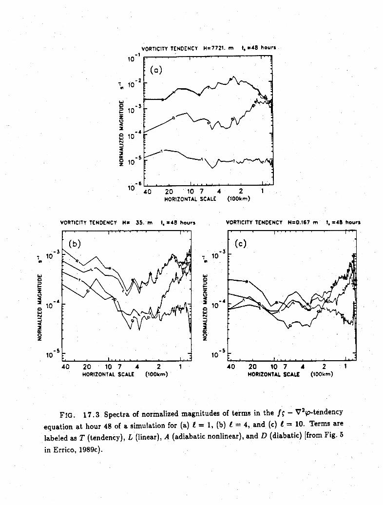
VORTICITY TENDENCY H=7721. m t, =48 hours

40 20 10 7HORIZONTAL SCALE

VORTICITY TENDENCY H= 35. m

40 20 10 7 4 2HORIZONTAL SCALE (100km)

t, =48 hours

0

t-

.20z

o

41O

z

1

VORTICITY TENDENCY H=0.167 m t, =48 hours

40 20 10 7 4 2HORIZONTAL SCALE (100km)

1

FIG. 17.3 Spectra of normalized magnitudes of terms in the f~ - Vp-tendency

equation at hour 48 of a simulation for (a) e = 1, (b) e = 4, and (c) t = 10. Terms are

labeled as T (tendency), L (linear), A (adiabatic nonlinear), and D (diabatic) [from Fig. 5

in Errico, 1989c).

-1

-2

-3

-4

-5

10

I' 10

, ,

= 10z04

o 10

I,.O

N

0 10z

-610 4 2 1

(100km)

-3

z

= 10

0

10 I4-fc2,,.I

z

10

N I

lO- i

II

I

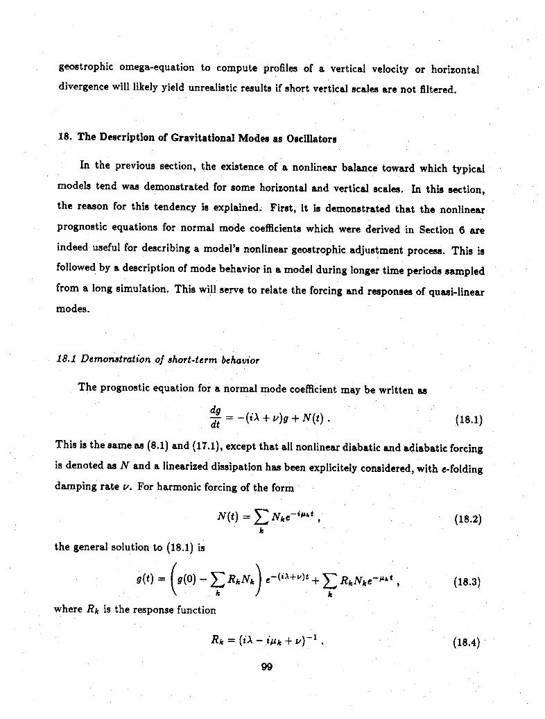
geostrophic omega-equation to compute profiles of a vertical velocity or horizontal

divergence will likely yield unrealistic results if short vertical scales are not filtered.

18. The Description of Gravitational Modes as Oscillators

In the previous section, the existence of a nonlinear balance toward which typical

models tend was demonstrated for some horizontal and vertical scales. In this section,

the reason for this tendency is explained. First, it is demonstrated that the nonlinear

prognostic equations for normal mode coefficients which were derived in Section 6 are

indeed useful for describing a model's nonlinear geostrophic adjustment process. This is

followed by a description of mode behavior in a model during longer time periods sampled

from a long simulation. This will serve to relate the forcing and responses of quasi-linear

modes.

18.1 Demonstration of short-term behavior

The prognostic equation for a normal mode coefficient may be written as

dg = -(iA + )g +N(t). (18.1)

This is the same as (8.1) and (17.1), except that all nonlinear diabatic and adiabatic forcing

is denoted as N and a linearized dissipation has been explicitely considered, with e-folding

damping rate v. For harmonic forcing of the form

N(t) = Nk (18.2)k

the general solution to (18.1) is

g(t) = (g(0)-E RkNk) e-(+v)t + E RkNkeC- , (18.3)V k / k

where Rk is the response function

Rk = (iA-ik + v)- . (18.4)

99

This is the same result as (8.3), except for consideration of v and the presence of more

than one forcing frequency.

Essentially, (8.1) has the form of the equation for the amplitude of a simple harmonic

oscillator which is damped and harmonically forced. In other words, the behavior of a

gravitational mode coefficient is similar in character to that of a spring or pendulum,

except that the "external forcing" acting on it may be quite complicated. Actually, (18.1)

is exact only in the sense that given N(t), g(t) is determined by that equation. From

(18.1) we learn about the effects of the nonlinear forcing of the mode, however we learn

nothing regarding the determination of N in general or the possible feedback of g on N

and subsequently on g itself (acting through N).

Although (18.1) and its solution (18.3) have simple forms, they do indeed describe the

behavior of many gravitational waves in models. As examples, we reproduce figures from

Errico and Williamson (1988) which show g(t) for some modes in a global NWP forecast

begun from a noninitialized analysis. The figures are presented as harmonic dials, which

are plots of real vs. imaginary parts of the g as functions of time on the same figure. They

are called harmonic dials because a harmonic function will appear as a circle (dial) on

the figure. Positive imaginary components are plotted in the bottom half plane so that

westward propagation appears as a clockwise sequence of points, as though the wave was

observed from above the north pole. Values of g were plotted every one-half hour, and

selected times (in hours from the initial time) are indicated in the figures.

Dials of four modes are presented in Figures 18.1a-d, corresponding to Figures 2a-d

in Errico and Williamson (1988). These are respective dials for: the t = 2, zonal wave

number 2, Kelvin mode; the external, largest meridional scale, zonal wave number 10,

westward propagating gravitational mode; the t = 4, 2nd largest meridional scale, zonal

wavenumber 1, westward propagating gravitational mode; and the t = 4, 12th largest

meridional scale, zonal wavenumber 9, westward propagating gravitational mode. In the

linearized model used to define them, these modes have respective periods 28.5, 3.4, 27,

100

(c)

(d)

60

FIG. 18.1 Harmonic dials for selected modes in a noninitialized CCM forecast

beginning from an ECMWF FGGE analysis: (a) I = 2, m = 2 Kelvin mode; (b) I =

1, first-symmetric, m = 10 westward-propagating gravitational mode; (c) t = 4, first-

antisymmetric, m= 1 westward-propagating gravitational mode; and (d) I = 4, sixth-

antisymmetric, m = 9 westward-propagating gravitational mode. The outer dotted circles

indicate magnitudes of 0.32, 0.048, 0.12 and 0.12 m s- 1, respectively. Crosses indicate

times labeled in hours after start of forecast [from Fig. 2 in Errico and Williamson, 1988].

Jib a

and 11.4 hours, and the noted directions of propagation refer to those in that linearized

model.

Behaviors of the presented external modes (Figs. 18.1a-b) appear to fit (18.3) quite

well. In particular, both have components with periods close to their linearized values,

although the mode in Figure 18.lb is noticeably slowed by the model's semi-implicit scheme

(Wiin-Nielsen, 1979; Errico 1984a) which has not been considered in the linearization but

which has a large effect on such otherwise fast modes. Both have damping, with the

smaller scale mode damped at a faster rate (approximately an amplitude e-folding time of

18 hours). Both appear to have quasi-stationary components based on the evidence that

the centers of the near circle during any period appear to be nearly concentric (to a crude

approximation) about a point offset from the graphs's origin. More detailed analysis and

discussion appears in Errico and Williamson (1988).

Behaviors of the internal modes (Figs. 18.1c-d) do not fit (18.3) as well as those of the

external modes, in the sense that regular damped propagation is less obvious. There appear

to be components with frequencies near the modes' linearized frequencies, but several

additional components of similar magnitude and period appear to be present also. This

complication may be considered as a consequence of less separation in frequency between

the nonlinear forcing and linearized frequency, or it may be considered a consequence of

the unrealism of the chosen basic state; i.e., the linearization has failed to distinguish the

modes which are more nearly independent in the nonlinear model (see, e.g., Errico, 1983).

The modes in Figure 18.1c-d actually may be linear combinations of modes which have

behaviors like those in Figure 18.1a-b, which then appear as several regular propagations

superimposed.

This last comment is based on some fundamental properties of normal-mode analysis.

As described in Section 6, we may write

cl = T (d- bl) , (18.5)

102

where d represents a set of data, b represents a basic state (such that d - b is a departure

from that state), and T- l represents a corresponding linear transform from data to a

set of mode coefficients c. The index 1 is used to contrast one basic state from another

(index 2) for which (18.5) would appear identically, except with a 2 replacing 1. Since d

is independent of the choice of b, a set C2 is related to cl by

c2 = T XT ll + TTlbl - b 2 (18.6)

The operator T lT 1, yields a matrix whose elements v describe the projection of one set

of mode structures on another; e.g., for mode q,

C2q = Vqj Ci (18.7)

plus terms involving bl and b 2 . If basic state 1 yields a set of regularly propagating

wave-like departures from that state, meaning that each Cly is associated with a distinct

frequency, then according to (18.7), a significantly different basic state 2 will likely yield

coefficients, each of which has several frequencies rather than a distinct single one. There-

fore, proper interpretation of time series of coefficients requires careful consideration of the

choice of basic state used to define the linearized eigenvalue problem.

18.2 Demonstration of long-term behavior

The component of g which depends directly on the initial condition g(O) eventually

becomes negligible since it is continuously damped. Therefore, after several damping

periods, the solution (8.3) is well approximated by

g(t) = E RkNkc At. (18.8)k

Although no longer explicit, (18.8) still depends on g(0), but only through its implicit

effect on the determination of N(t) and therefore on Nk.

Solution 18.8 emphasizes the importance of the response function. The magnitude

of the response of g at any frequency Ik is proportional to not only the magnitude of

103

11210

1010

8

610

410

m= 1 n= 0 1=1 EG Pr = 33.0_ u l I 11fi 1l' I I I"' -' ' '

-_-

m1* \

r. "i

m . I I I - . , , III | I

102 10PERIOD (hours)

100

FIG. 18.2 Response function R for the forcing of eastward propagation (solid) andwestward propagation (dashed) for a wave with resonance at a 33 hour period (eastward

direction) and linear e-folding damping period of 5 days [from Fig. 16 in Errico, 1989a].

(,s

cv(nI

0o

z0

0

L.

LiJC)z0a.(n,LiJcx

the forcing at that frequency, but also to the magnitude of the response function at that

frequency. The latter magnitude is greater the closer Ak is to A; i.e., the closer the forcing

is to resonance. An example of a response function appears in Figure 18.2 for a mode with

a linearized model period of 33 hours with eastward propagation and assumed e-folding

damping period of 5 days (without damping, R would be infinite at resonance).

Harmonic dials of four modes from 16 days near the end of a 1000-day simulation are

shown in Figure 18.3a-d. These are taken from Errico (1989a; his Figu res pectively)

and may be described as: (a) the fifth largest meridional scale, zonal wavenumber 7,

external westward propagating gravitational mode (3.1 hour resonant period); (b) the

zonal wavenumber 1, external Kelvin mode (33 hour resonant period); (c) the tenth largest

meridional scale, zonal wavenumber 4, t = 5 westward propagating gravitational mode

(14 hour resonant period); and (d) the zonal wavenumber 4, t = 4 Kelvin mode (52.2 hour

resonant period). Asterisks on the dials are separated by one-day periods. The simulation

is sufficiently long so that the presented behaviors are responses to forces acting upon the

modes rather than explicit effects of initial conditions. The simulation was performed with

the NCAR CCM1.

The mode in Figure 18.3a is representative of all fast modes (resonant periods less

than 12 hours) in the simulation. It has a strong stationary component (presumably

a topographic effect) and a significant quasi-stationary component. Superimposed are

some small wiggles, which are near resonant gravitational components (as evidenced by

Figure 18.4a). The remaining modes (Figures 18b-d) show significant wave-like behavior

with periods not much different than the mode's resonant periods.

Power spectra of the modes in Figure 18.3a-d are presented respectively in

Figures 18.4a-d. These are determined by removing linear trends from the mode coefficients

during a 64-day period and performing Fourier analysis on the remainders. Solid lines

indicate westward propagating components; dashed lines indicated eastward components.

Note that although in the linearized model used to define the modes, each mode

105

m= 7 n= 4 1=1 WG Pt= -3.1

. . i 1 ! ! !., . . , I . .i

-0.08:

. ~ ~~~~~~~~ .

.

~~~~~~~~~. .

..

~~~~...

· -. i i i i i m0.08

_ i

- 0.08

m= 4 n= 9 1=5 WG P,= -14.0 m= 4 n 0 1=4 EG P, = 52.2

FIG. 18.3 Harmonic dials of four modes obtained near the end of a long climate

simulation: (top left) third-symmetric, m = 7, e = 1 westward-propagating gravitational

mode; (top right) m = 1, e = 1, Kelvin mode; (bottom left) fifth-antisymmetric, m =

4, t =5 westward-propagating gravitational mode; and (bottom right) m = 4, t = 4

Kelvin mode. Asterisks indicate times which are multiples of 24 hours, axes have units

m/s, and a-c show behavior for 16 days and d for 64 days [from Fig. 1-4 in Errico, 1989aJ.

rn.=1 n=0 1= EG , =33.0

-0.08 - ...

. I

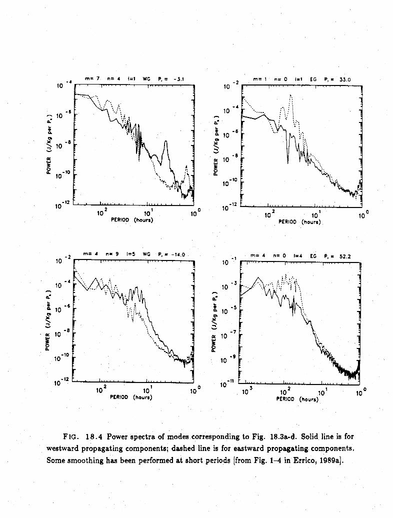
m= 1 n= 0 1=1 EG P, = 33.0

10 10PERIOD (hours)

1-2

-410

a.k.

. 10

a 10wa: 10

ao

100

-6

-8

-1010

-1210

102 10PERIOD (hours)

1=5 WG P,= -14.0 m= 4 n= 0 1=4-1

10

10

^,0-7· .1

a.

10= 10

10 110

EG P, = 52.2

10 101PERIOD (hours)

FIG. 18.4 Power spectra of modes corresponding to Fig. 18.3a-d. Solid line is for

westward propagating components; dashed line is for eastward propagating components.

Some smoothing has been performed at short periods [from Fig. 1-4 in Errico, 1989a].

10

-6- 1U

o,

a 10

sa>

-8

-10

0-1210

10m= 4 n= 9

-410

100

- 60 -6a, 10

-8

0 0.-10

-l

10°

m-7 n = W ,= -.-4

_ -2

propagates in a certain direction only, in the nonlinear model, there is no unique as-

sociation. Rather, the propagation characteristics of a mode depend on the strength and

propagation characteristics of its various forcings, but only in one direction does a resonant

response exist.

The spectra quantitatively reveal the qualitative comments made earlier regarding the

dials. In particular, relative peaks are observed near the resonant periods of all modes,

but in the case of Figure 18.a, the peak is still small. The relative peak at shorter period

which occurs in the component which travels in the direction opposite that of the resonant

component is due to resonance of a corresponding time-computational mode produced by

the model's semi-implicit time scheme.

Note that no band averaging has been performed for these figures, and therefore

the energy within each period-band of components is proportional to the area under the

curve for that band and a factor which approximately varies as the inverse of the period.

Therefore although a peak may be small, it may integrate to a large portion of energy.

Clearly, for the internal modes shown, there is substantial energy in the near-resonant

bands. This is entirely due to forcing in the model.

As further evidenced by Errico (1989a), a significant portion of the forcing which

is reponsible for excitation of wave-like behavior is the model's convective heating. In

other words, the convection primarily acts to create relatively fast, unbalanced components

rather than slow balanced components. The key word here is "relatively", which denotes

a comparison between forcing and resonant periods. The tropical internal modes typically

have resonant periods of longer than one day. For convective forcing to instead drive

balanced components of these modes, it would be required to have the same magnitude

and location for periods of several days to weeks, which is exceedingly rare (especially for

the Kelvin modes for which months would be required). The analysis in Errico (1989a)

demonstrates that the time scale of the modes is in part explained by the time scales of the

various forces acting on them. If the time scale of forcing is predominately an advective

108

one, and if there is sufficient damping to limit more weakly driven but resonant responses,

then the time scale of gravitational modes will be an advective, rather than inertial, one.

The same time scale will be observed for the ageostrophic fields of 6 and fo - V 2 p since

they physically describe the gravitational modes. This explanation is only partial, because

the question of why particular time scales of the dynamic fields are observed has only been

shifted to the question of why the forcing has an advective time scale. In particular, since

the forcing actually depends on the ageostrophic components themselves, it at least has

the potential to have significant high frequency components. Of course, the observation

that the time scales of the ageostrophic fields are advective strongly indicates that the

forcing acting on them is predominantly advective, as mentioned by Charney (1955). The

nature of the forcing acting on the modes will be discussed in the following section.

19. Mode Forcing, Interaction, and the Slow Manifold

Charney (1955, 1973) presents brief outlines of why the atmosphere is quasi-geostropic.

Essentially, the primary external forcing acting on the atmosphere is solar heating which

is characterized by a predominately large space scale (cooling at the poles; heating at the

equator) and long time scale (the latitudinal heating contrast is always present to some

large degree). Other time and space scales are associated with solar heating (e.g., the time

and space scales of clouds passing overhead), but the components at these other scales

are either weaker or affect much smaller scales than we are characterizing (essentially we

are discussing the synoptic and mesoscales, and medium to large equivalent depths). The

response to the primary forcing has the same space and time scales as that forcing, resulting

in strong zonal winds aloft in the midlatitudes which have a significant seasonal component

but which are otherwise always present. These winds are geostrophically balanced, however

they are unstable with respect to small nonzonal perturbations (Charney, 1948; Eady

1948). The perturbations which grow most rapidly are the quasi-geostrophic ones, resulting

in propagating quasi-geostrophic waves. These waves are also unstable with respect to

109

other quasi-geostrophic perturbations (Lorenz, 1972; Kim 1978), yielding many scales of

quasi-balanced fields. If they were also significantly unstable with respect to gravity waves,

we would expect to see more gravity waves, so Charney presumed they were not. Also,

some dissipation is required to remove any significant energy which may otherwise creep

into gravity waves, so that quasi-geostrophic balance is maintained.

In the following subsections various aspects of Charney's explanation will be dis-

cussed in greater detail. In Section 19.1 the stability of geostrophic waves to ageostrophic

disturbances will be discussed. Also, the requirement of dissipation for maintenance of

quasi-geostrophic conditions will be discussed. In Section 19.2 the capability of mode

interactions to result in a "slow" set of solutions will be discussed, along with higher-order

balance conditions.

19.1 Stability and Dissipation of Geostrophic Waves

Charney's (1955) conclusion that geostrophic waves are stable with respect to gravity-

wave perturbations was actually conjecture based upon the observations of the lack of

gravity wave activity rather than a demonstration of that stability. That geostrophic

waves are unstable with respect to other geostrophic waves has been demonstrated by

many (Lorenz, 1972; Kim, 1978; Gill, 1974; et al.), however those studies have typical used

quasi-geostrophic models which exclude examination of gravity waves.

Errico (1981) examined the stability of gravity waves in a periodic two-level f-plane

primitive equation model. He used an approach similar to that of Lorenz (1972) and Lin

(1980) except he computed interaction coefficients for both gravity and Rossby waves.

The basic states were single geostrophic waves (either barotropic or baroclinic), analogous

to the rotational modes for the model in Section 3, superimposed on a statically stable

110

horizontally uniform state. In his model, these states were stationary solutions to the

model equations.

Growth rates for quasi-geostrophic wave perturbations were asymptotically propor-

tional to the amplitude of the basic state waves as smaller amplitudes were considered. In

other words, for a basic state amplitude of order Rossby number e «<< 1, the growth rate

was proportional to e. Similar scaling had been obtained by Lorenz (1972) and Lin (1980).

However, ageostrophic gravity-wave perturbations also grew, but at rates proportional to

c2. For small values of c which would characterize the atmosphere, the latter growth rates

were significantly smaller than those for the quasi-geostrophic perturbations, such that

weak linear dissipation would have effectively eliminated the gravity-wave growth but not

the quasi-geostrophic growth.

A need for dissipation may also be inferred from consideration of gravity waves as

linear oscillators. In such a simple description of their dynamics, their response functions

are infinite at resonance without dissipation, and therefore any forcing at the resonant

frequency yields an infinite response. Of course, nonlinear dynamics actually places con-

straints on the response (since energy is conserved under adiabatic conditions), but the

simple description of the waves in previous sections has ignored the feedback of the modes

on the nonlinear forcing which acts to limit adiabatic resonant responses.

The need of dissipation for maintenance of quasi-geostrophic conditions was further

highlighted in a study by Errico (1984c), which showed that energy is indeed transferred

from geostrophic modes to gravity waves if no dissipation is present as a stabilizing

effect. He examined both long and short term solutions of a multilevel primitive equation

model which had no diabatic forcing or dissipation. Importantly, the only invariants in

111

his model were the horizontal mean static stability and a quadratic form of the total

(kinetic plus available potential) energy. Initial conditions were obtained from a damped

and slowly forced solution which was approximately quasi-geostrophic in character, with

approximately 100 times more energy in geostrophic modes compared with gravity waves

and the gravity waves characterized by balance rather than rapid propagation. He showed

that energy was slowly transferred from the geostrophic modes to gravity waves and

that the resulting gravity waves were characterized by propagation at the speed of free

linearized waves. The final result was an equal partitioning of the quadratic energy among

all the modes. In fact, since there were 5/3 as many gravitational modes compared with

geostrophic modes, the accumulated energy of the former was 5/3 that of the latter. Such

a result had been expected using statistical-mechanical arguments, but it remained to be

demonstrated.

19.2 Slow Manifold

A presentation of the theory and application of nonlinear normal mode initialization

would not be complete without discussion of the concept of a "slow manifold" (Leith,

1980). However, due to remaining questions about the possible existence of a slow manifold

(Lorenz, 1980; Errico, 1982; Warn and Menard, 1986; Lorenz, 1986; Vautard and Legras,

1986; Lorenz and Krisnamurthy, 1987) and even questions regarding its proper definition,

discussion here will be brief. Also, irrespective of the existence of a slow manifold, the

previous 18 sections demonstrate the utility of the theory of NNMI, and even the concept

of a slow manifold has had proven utility (e.g., Tribbia, 1982; Daley, 1980; Williamson and

Daley, 1983).

The description of the slow manifold uses the language of dynamic systems theory. A

state of the system or model is defined by the location of a point in a multi-dimensional

112

space whose coordinates are values of the independent variables describing the system (e.g.,values of all dynamic fields at all grid points, or values of coefficients of all fields for allfunctions and levels in a spectral description). The state of the system changes with time,

describing a trajectory in state space: this can be considered a curve (or point) in state

space, where each point is associated with one (or more) times. A manifold is a smaller

dimensional subspace (e.g., a 2-dimensional surface imbedded in a 3-dimensional space).

The slow manifold has the properties that: 1) the gravitational mode coefficients

or field components may be determined from the rotational mode coefficients or fieldcomponents (it therefore has 2/3 the dimensionality of the complete state space if this

property applies to all gravitational modes); and 2) solutions are slow in some sense, and

in particular, freely-appearing gravity waves are absent. Some solutions to primitive equa-

tions models have the appearance of lying within slow manifolds, however that appearance

may be deceptive if free gravity wave behavior is very weak (e.g., as in Lorenz (1980) asexplained by Krisnamurthy (1985)). Also, the destruction of a slow manifold may occur dueto resonant responses of gravity waves forced by possible high-frequency numerical errors,

such as due to random or systematic round-off. Schemes used to compute gravitational

modes from rotational modes may fail to converge due to the algorithms used or numerical

accuracy available. For these reasons either the existence or nonexistence of a truly slowmanifold is hard to prove.

The slow manifold is often schematically represented by the diagram in Fig. 19.1.

There, the multidimensional state space has only two dimensions: the abscissa (R) and

ordinate (G) denote magnitudes of single rotational and gravitational mode coefficients

respectively. The parabola (S) represents a slow manifold which is quadratic in the

rotational mode amplitude: for any value of the rotational mode coefficient, that for the

gravitational mode coefficient is uniquely determined for any point on the manifold. The

line labeled D represents a data manifold of smaller dimension (here 1) than the complete

state space: all combinations of R and G along D are consistent with the data. This lower

113

dimensionality of D reflects the fact that the atmospheric or model state is typically under-

determined by data alone (Lorenc, 1986). By means of diagrams such as 19.1, relationships

between data, initialization, and model behavior can be graphically yet simply described

(e.g., Williamson and Daley, 1983; Tribbia 1982; Daley, 1980). Of course, such diagrams

are necessarily highly simplified, and any inferences drawn from them must be confirmed

by more rigorous analysis of the actual multi-dimensional model equations themselves.

As a trivial example of the use of a schematic slow manifold diagram, the relationships

among data, linear initialization, and rotational-mode constrained nonlinear initialization

are represented in Fig. 19.1. The point (or system state) labeled 1 is the result of a

linear initialization applied to the data: the gravitational mode has 0 amplitude and R

is determined by the projection (interception) of D. Point 2 is the result of a rotational-

mode constrained NNMI: the value of R is the same as for point 1 and the value of

G is consistent with both that value of R and the balance expressed by curve S. The

line W indicates the unbalanced gravitational wave component which would result from

performing a linear initialization (i.e., from initializing the system at point 1 rather than

the balanced point 2). Given perfect but insufficient data, the state denoted by point 3 is

the one which an ideal initialization should yield: it is consistent with both the data (D)

and the balance condition (S). Note that rotational-mode constrained NNMI has failed

to yield this desired state (point 3 is distinct from point 2), and instead its result is not

consistent with the data provided. In order to yield state 3 as its result, the constraint

on R in the usual NNMI procedure must be relaxed, as in variational NNMI methods

(e.g., Daley, 1980; Tribbia, 1982). All these relationships have been compacted neatly in

Fig. 19.1.

Questions regarding the existence of a slow manifold concern the degree to which

high-frequency behavior of gravitational modes occurs and the accuracy with which the

gravitational mode coefficients may be determined from only rotational mode coefficients

114

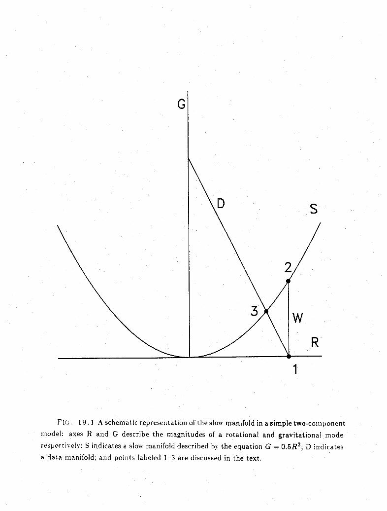
G

D -S

W

R

1

F(IG. 19.1 A schematic representation of the slow manifold in a simple two-conmponentmodel: axes R and G describe the magnitudes of a rotational and gravitational moderespectively: S indicates a slow manifold described by the equation G = 0.5R 2 ; D indicatesa data manifold; and points labeled 1-3 are discussed in the text.

(condition 1 for the definition of the slow manifold above). For a truly slow manifold, the

former modes are uniquely determined by the latter modes, with perfect accuracy, but

it is not clear how much high-frequency behavior there can be. There is some evidence

and speculation that a finite Rossby number implies some residual "noise" in gravitational

components (Lorenz, 1980; Errico, 1982; Warn and Menard, 1986; Lorenz, 1986; Vautard

and Legras, 1986; Lorenz and Krisnamurthy, 1987), but some counter examples have also

been presented (Tribbia, personal communication).

Finally, it should be noted that higher-order balance schemes are possible. These

do not consider that dg/dt = 0, but instead use the condition that dg^/dtn = 0 for

some n > 1, or use some estimates of dgn /dt n (n > 1) based on slowly propagating

components only. These have been discussed by Baer and Tribbia (1977), Lorenz (1980),

Machenhauer (1982), Tribbia (1984), Temperton (1988), and Errico (1989b). Regarding

numerical weather prediction, in most cases they change subsequent forecasts very little

with respect to other analysis or model errors, because order en adjustments are extremely

small for small E (Rossby number) and large n. However, these higher-order schemes have

considerable theoretical interest.

116

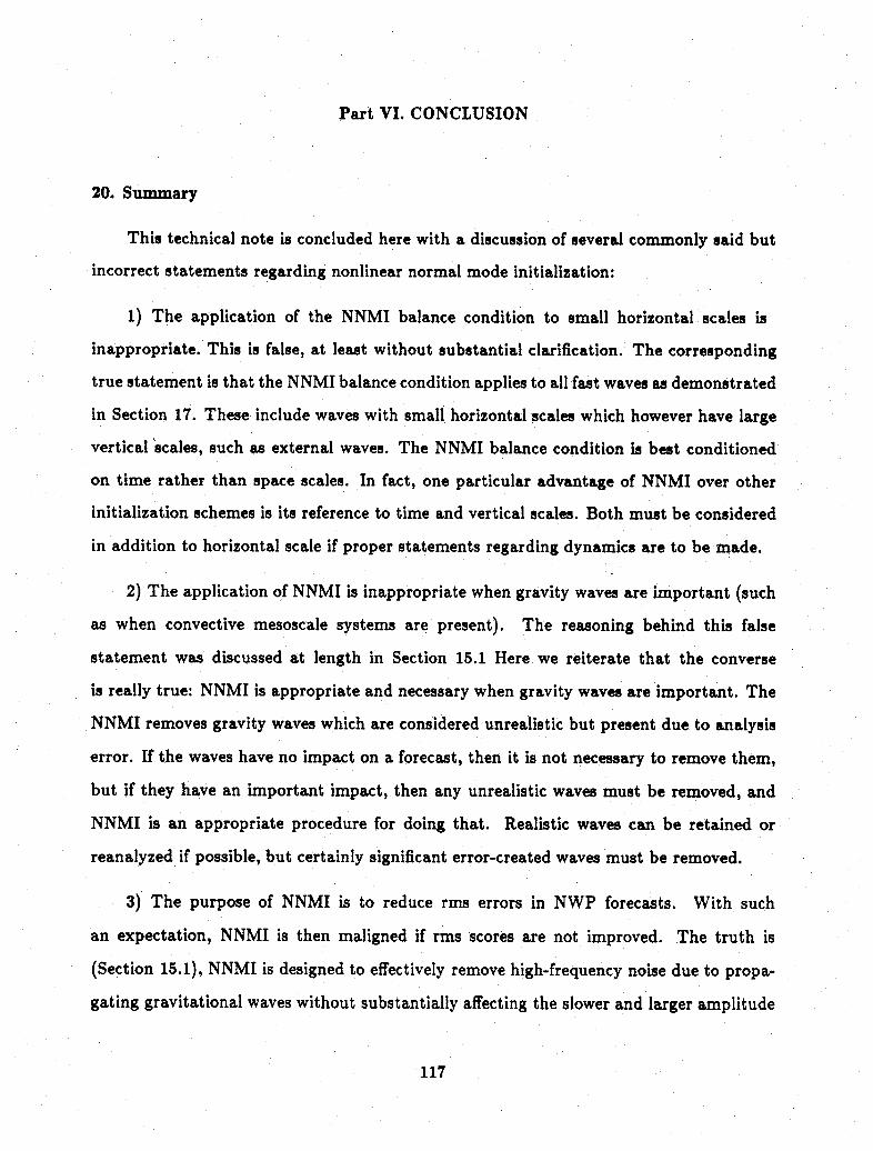
Part VI. CONCLUSION

20. Summary

This technical note is concluded here with a discussion of several commonly said but

incorrect statements regarding nonlinear normal mode initialization:

1) The application of the NNMI balance condition to small horizontal scales is

inappropriate. This is false, at least without substantial clarification. The corresponding

true statement is that the NNMI balance condition applies to all fast waves as demonstrated

in Section 17. These include waves with small horizontal scales which however have large

vertical scales, such as external waves. The NNMI balance condition is best conditioned

on time rather than space scales. In fact, one particular advantage of NNMI over other

initialization schemes is its reference to time and vertical scales. Both must be considered

in addition to horizontal scale if proper statements regarding dynamics are to be made.

2) The application of NNMI is inappropriate when gravity waves are important (such

as when convective mesoscale systems are present). The reasoning behind this false

statement was discussed at length in Section 15.1 Here we reiterate that the converse

is really true: NNMI is appropriate and necessary when gravity waves are important. The

NNMI removes gravity waves which are considered unrealistic but present due to analysis

error. If the waves have no impact on a forecast, then it is not necessary to remove them,

but if they have an important impact, then any unrealistic waves must be removed, and

NNMI is an appropriate procedure for doing that. Realistic waves can be retained or

reanalyzed if possible, but certainly significant error-created waves must be removed.

3) The purpose of NNMI is to reduce rms errors in NWP forecasts. With such

an expectation, NNMI is then maligned if rms scores are not improved. The truth is

(Section 15.1), NNMI is designed to effectively remove high-frequency noise due to propa-

gating gravitational waves without substantially affecting the slower and larger amplitude

117

behavior of the dynamic fields (except possibly under strong diabatic conditions). After

a period of time, other mechanisms remove gravity waves in the absence of initialization.

Therefore, after an adjustment period, initialized and noninitialized forecasts should ap-

pear very similar. In fact, that is one important test of a correct application of NNMI

software. In contrast to its lack of a direct effect, NNMI has significantly improved forecasts

by creating better, more noise-free, background (or first guess) fields for use in the analysis

of atmospheric data when those fields are produced by previous short-term model forecasts,

such as in a forecast, analysis, initialization cycle. Although fast gravity waves have only

small dynamic effects on slower components of either gravity waves or rotational modes,

slow components can be significantly impacted by affecting their analysis.

4) NNMI is just another "trick" to remove forecast noise, and therefore is a subject

of interest only regarding NWP modeling. This is false, as the previous 19 sections have

been intended to demonstrate. Rather, the theory of NNMI is as fundamental as quasi-

geostrophic theory, and in fact explains the basis for that theory (Sections 16-19). It

elegantly infuses linear concepts into nonlinear contexts, for example regarding nonlinear

geostrophic adjustment (Section 8). For these reasons, the theory of NNMI should be part

of a basic meteorological curriculum in atmospheric dynamics at the graduate level.

5) With the advent of diabatic NNMI, initialization is a solved problem. The truth is

that NNMI has been somewhat hurt by its so successful and easy application. There

are many remaining problems. Attention has been primarily focused on noise in the

surface pressure field, at the exclusion of attention to internal waves, especially in the

tropics. The effects of diabatic processes has been mostly misunderstood (Section 15.3),

and modifications to NNMI procedures have been often poorly diagnosed (Section 15.2).

There is much work yet to be done, however the greatest potential for normal modes is

probably as a diagnostic tool (e.g., as in Section 17) especially where fast and slow, or

geostrophic and ageostrophic fields are to be distinguished.

118

APPENDIX A: List of Mathematical SymbolsThe section number where the symbol first appears is indicated in parenthesis. Some

symbols which are used in only a single section are excluded from this list.

a Structure functions of the spectral components of normal modes (4.3).a A generic field (3).

A Shorthand for the adiabatic nonlinear terms acting on the mode coefficients (17).c The phase speed of a gravity wave (4.3) or a coefficient (complex amplitude)

of a generic normal mode (17).

D Shorthand for the diabatic terms acting on a field or mode, as indicatedby a subscript (3.1).

P The Kronecker delta function (4.1).

E The total kinetic plus (a quadratic form of) available potential energy,per unit mass (3.2).

f The Coriolis parameter (3).

fo A constant or mean Coriolis parameter (3).

g The acceleration of gravity (3.1) or a normal mode coefficient (complex amplitude)of a gravitational mode (4.3).

g' The coefficient of a conjugate gravitational mode (4.3).G The typical magnitude of a gravitational mode coefficient (7).h The phase speed of a gravitational mode with fo negligible (4.3).H An equivalent depth of a vertical mode (4.1).i The square root of -1 (4).

j An index for a normal mode (17).

L A typical length scale (7).

LF A length scale which describes the periodicity of the model domain (3).

LR The Rossby radius of deformation (5.1).

Lx A wavelength in the z direction (4.2).

Ly A wavelength in the y direction (4.2).

I An index denoting a vertical mode (4.1).Shorthand for the 3-dimensional linear operator acting on the dynamic fields (4).

£c A linear operator describing the coupling between fields (4).A linear operator (acting on x dependence only) (4).

119

A linear operator (acting on y dependence only) (4).

0 - a linear operator (acting on a dependence only) (4).

m A wavenumber in the x direction (4.2)

n A wavenumber in the y direction (4.2)

N Shorthand for the nonlinear terms acting on the mode indicated by a subscript,with dependence on modes indicated in parenthesis (6).

N The magnitude of an oscillating form of N (8).

Shorthand for the nonlinear terms acting on a field (6).

p The hydrostatic pressure (3.1)

Pa The hydrostatic pressure at the earth's surface (3.1)

p A mean value of the surface pressure (3.2)

P A linearized potential vorticity (10)

P A Fourier transform coefficient of horizontal variations of In (p,/p) (11).

q Shorthand for the set of scales m, n, t (4.3).

r The coefficient (complex amplitude) of a rotational mode (4.3).

R The gas constant for dry air (3.1).

Rk The response function of a mode to forcing at a frequency fk (18).

8 The x-dependence of a mode's structure (4).

' The y-dependence of a mode's structure (4).

S A factor for simplifying notation (4.3).

t Time (3.1).

T Temperature (3.1).

T A basic state, horizontally uniform temperature (3.2).

T I A departure of T from T (3.2).

u The velocity in the x direction (3.1).

A basic state value of u (equal to zero) (3.2).

u A vertical mode coefficient of u (4.1).

u A Fourier transform coefficient of horizontal variations of u (4.1).

U A typical magnitude for scaling velocity (7).

v The velocity in the y direction (3.1).

V A basic state value of v (equal to zero) (3.2).

v A vertical mode coefficient of v (4.1).

v A Fourier transform coefficient of horizontal variations of v (4.2).

120

x A direction which increases eastward (3).

y A direction which increases northward (3).z A function which describes the vertical structure of a mode (4.1).Z A matrix whose columns are vertical modes of vertically-discrete model (12).a A coefficient which describes some mode interactions (6), or a field

proportional to the ageostrophic (i.e., linearly unbalanced portion of) vorticity (17.2)./3 A coefficient which describes some mode interactions (6).7 f A coefficient which describes some mode interactions (6).r A static stability parameter (3.1).

6 The horizontal velocity divergence (3.1).

C A scaling parameter or Rossby number (7).

The vertical component of vorticity (3.1)./c The ratio of the gas constant to the specific heat of dry air

for an isobaric process (3.1).

A The frequency of a normal mode (4.3).

A Shorthand for the linear operator acting on normal mode coeffients (6)./~ The frequency of a harmonic forcing function (8).v A coefficient of linear dissipation (18.1).

a A terrain-following vertical coordinate (3.1).r The vertical intergral operator in the linearized tendency equation

for pseudo geopotential (3.2).

T Shorthand for the eigenfunctions of the operator £ (6).

f > The hydrostatic geopotential (3.1).

<by The geopotential height of the surface topography (3.1).

The pseudo geopotential (3.2).

A vertical mode coefficient of p (4.1).

A Fourier transform coefficient for horizontal variations of , (4.2).~, s A horizontal mean value of b, (3.2).

fl A scaling parameter for time differentials (7).

V 2 The horizontal Laplacian operator (10).

121

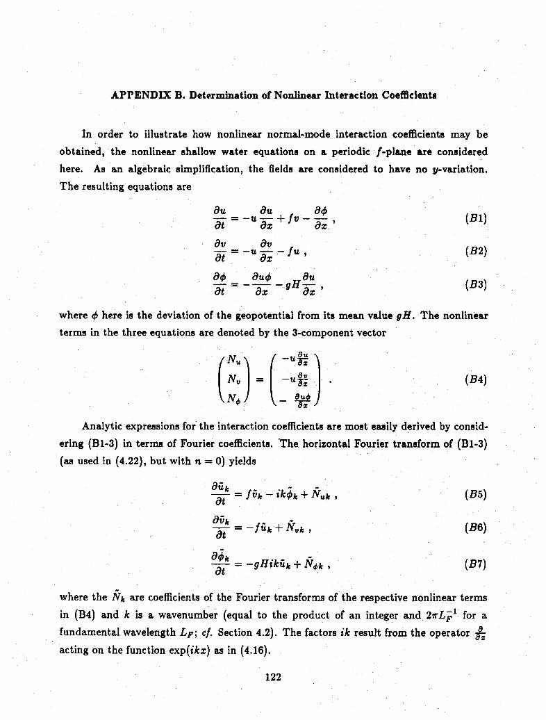
APPENDIX B. Determination of Nonlinear Interaction Coefficients

In order to illustrate how nonlinear normal-mode interaction coefficients may be

obtained, the nonlinear shallow water equations on a periodic f-plane are considered

here. As an algebraic simplification, the fields are considered to have no y-variation.

The resulting equations are

au au a6i: -"~ + f"V - (El)at ax

9= -u -_fu, (B2)at =az-Ox

8a+=-S a -0U4 Og (B3)

where < here is the deviation of the geopotential from its mean value gH. The nonlinear

terms in the three equations are denoted by the 3-component vector

NU _ 8.

N V = |- U _ * (B4)

Analytic expressions for the interaction coefficients are most easily derived by consid-

ering (Bl-3) in terms of Fourier coefficients. 'The horizontal Fourier transform of (Bl-3)

(as used in (4.22), but with n = 0) yields

= fisk-ikk + Nk, (B5)

= =-fi + Nvk, (B6)

=t -- gHikuk + ANk, (B7)

where the Nk are coefficients of the Fourier transforms of the respective nonlinear terms

in (B4) and k is a wavenumber (equal to the product of an integer and 27rL- 1 for a

fundamental wavelength LF; cf. Section 4.2). The factors ik result from the operator .

acting on the function exp(ikx) as in (4.16).

122

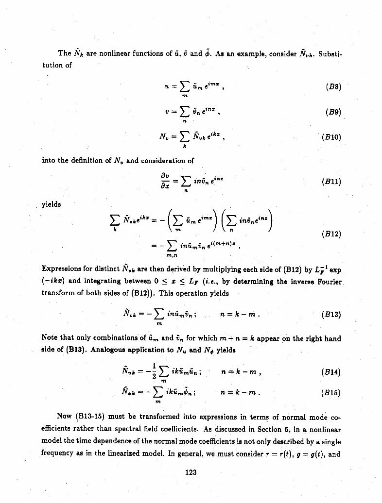
The Nk are nonlinear functions of u, v and 4. As an example, consider Nvk. Substi-

tution of

u"= E Zi m mz, (B8)m

"v E v c-" (B9)n

N = Nvk ek , (B10)k

into the definition of Nv and consideration of

: ,=V E invn einz (Bil)n

yields

N,,ke =- (z m i)n invne )bfc~~ A~m / V~~~n )(B12)

=-E intumvn ei (m + n )z .m,n

Expressions for distinct Nvk are then derived by multiplying each side of (B12) by L- 1 exp(-ikx) and integrating between 0 < z < LF (i.e., by determining the Inverse Fouriertransform of both sides of (B12)). This operation yields

Nvk = - iniimn ; n = k- m . (B13)m

Note that only combinations of um and ,i for which m + n = k appear on the right handside of (B13). Analogous application to Nu and No yields

uk =- Z ikiumUn; n = k-m, (B14)m

Nk = t ikumqn; n =k-m. (B15)m

Now (B13-15) must be transformed into expressions in terms of normal mode co-

efficients rather than spectral field coefficients. As discussed in Section 6, in a nonlinearmodel the time dependence of the normal mode coefficients is not only described by a singlefrequency as in the linearized model. In general, we must consider r = r(t), g = g(t), and

123

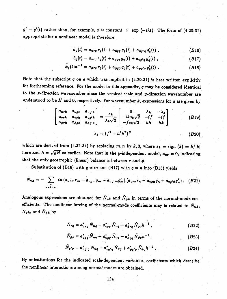
g' = g'(t) rather than, for example, g = constant x exp (-iAt). The form of (4.29-31)appropriate for a nonlinear model is therefore

uq(t) = aurq rq(t) + augq gq(t) + aug'q 9q(t) , (B16)

vq(t) = avrq rq(t) + avgq gq (t) + avgq g(t) , (B17)

q (t)h- l aqrq(t) +( t) + aggiq g(t) a (1B18)

Note that the subscript q on a which was implicit in (4.29-31) is here written explicitlyfor forthcoming reference. For the model in this appendix, q may be considered identicalto the :-direction wavenumber since the vertical scale and y-direction wavenumber areunderstood to be H and 0, respectively. For wavenumber k, expressions for a are given by

[ urk augk auglk 0 Ak -Afk|avrk avgk avg'k = --a/| -ikSkv2 -if -if (B19)Gark a 0gk ag'k J L -fsk /2 hk hk

Ak = (f 2 +h2k2) 4 (B20)

which are derived from (4.32-34) by replacing m,n by kO, where Jk = sign (k) = k/lIkIhere and h = as earlier. Note that in the y-independent model, aur = 0, indicatingthat the only geostrophic (linear) balance is between v and qb.

Substitution of (B16) with q = m and (B17) with q = n into (B13) yields

Nvk = - in (aurmrm + augm9m + aug,9mg) (avmorn + avongn + avgingf) * (B21)n=-m

Analogous expressions are obtained for Nuk and Nk in terms of the normal-mode co-efficients. The nonlinear forcing of the normal-mode coefficients may is related to Nuk,Nvk, and N,^ by

Nrq = arq Nuq + a;rq Nvq + a^,q Nqh-l , (B22)

Ngq = aggq Nuq + a;gq Nvq + agq Nqh 1 , (B23)

NgIq = a*gsq Nuq + a*iq Nvq + a*,qI Nqh . (B24)

By substitutions for the indicated scale-dependent variables, coefficients which describethe nonlinear interactions among normal modes are obtained.

124

As an example of the determination of a specific interaction coefficient, consider theforcing of rk by all nonlinear terms involving products of r and g (throughout this appendix,we will continue to distinguish g from g'). The contributions to Nuk, Nvk and Nlk by

products rmgn for the present model are Nk = 0, and

Nvk (rg) = - in augmavrnrngm , (B25)m

n = k-m

NO (rg)=- - ikh ausmaornrngm , (B26)in

n=k-m

where aurk = 0 has been used. Substitution of these expressions into (B22) yields thenonlinear interaction coefficient which describes the forcing of rotational modes by the

interaction of rotational modes with the class of gravitational modes corresponding to g

(as contrasted with those corresponding to g'):

Nrk (rg) =- aum (inar vaur + ikaornark) rgm . (B27)m

, = n=l-m

Finally, consideration of (B19-20) yields

N^k (rg ̂ ^ ik m (f2+gH(k-m)2),Nrk (rg) - rk-m g,,. (B28)

E [ d |m| f2+ gnk2

The expression in brackets is the nonlinear interaction coefficient. It depends on the

scales k, m, n = k - m, as well as on f and H. Analogous expressions with other scaledependencies may be derived for other mode combinations.

125

REFERENCES

Andersen, J.H., 1977: A routine for normal mode initialization with non-linear correction

for a multi-level spectral model with triangular truncation. ECMWF Internal Report

No. 15, 41pp. [Available from the European Centre for Medium Range Weather

Forecasts, Shinfield Park, Reading RG2 9AX, England.]

Anthes, R.A., E. -Y. Hsie and Y. -H. Kuo, 1987: Description of the Penn State/NCAR

Mesoscale Model Version 4 (MM4). NCAR Technical Note, NCAR/TN-282+STR, 66

pp. [Available from the National Center for Atmospheric Research, P.O. Box 3000,

Boulder, CO 80307, USA]

Baer, F., 1977: Adjustments of initial conditions required to suppress gravity oscillations

in nonlinear flows. Contrib. Atmos. Phys., 50, 350-366.

Baer, F. and J. Tribbia, 1977: On complete filtering of gravity waves through nonlinear

initialization. Mon. Weather Rev., 105, 1536-1539.

Ballish, B. 1981: A simple test of the initialization of gravity modes. Mon. Weather Rev.,

109, 1318-1321.

Barker, E.H., 1982: A comparison of two initialization methods in data assimilation. Ph.D.

Thesis, Naval Postgraduate School, Monterey, CA, 151 pp. [Available from Naval

Environmental Prediction Research Facility, Monterey, CA 93940 USA].

Bengtsson, L., 1975: Four-dimensional assimilation of meteorological observations. CARP

Publication Series, No. 15, WMO, 76 pp. [Available from UNIPUB, New York, NY

10010, U.S.A.]

126

Bengtsson, L., 1981: Current problems in four-dimensional data assimilation. Data As-

similation Methods, ECMWF Seminar '1980, 195-217. [Available from the European

Centre for Medium Range Weather Forecasts, Shinfield Park, Reading RG2 9AX,

England.]

Bengtsson, L., M. Ghil, and E. Kall6n, editors, 1981: Dynamic Meteorology: Data Assim-

ilation Methods. Springer-Verlag, 340 pp.

Blumen, W., 1972: Geostrophic adjustment. Rev. Geophys. Space Phys., 10, 485-528.

Bourke, W., and J. L. McGregor, 1983: A nonlinear vertical mode initialization scheme

for a limited area prediction model. Mon. Weather Rev., 111, 2285-2297.

Branstator, G., 1989: Low frequency patterns induced by stationary waves. J. Atmos.

Sci., in press.

Briere, S., 1982: Nonlinear normal mode initialization of a limited area model. Mon.

Weather Rev., 110, 1166-1186.

Carr, F. H., R. L. Wobus, and R. A. Petersen, 1989: A synoptic evaluation of normal mode

initialization experiments with the NMC Nested Grid Model. Mon. Weather Rev., in

press.

Carrier, G. F., and C. E. Pearson, 1976: Partial Differential Equations: Theory and

Technique. Academic Press.

Charney, J. G., 1948: On the Scale of Atmospheric motions. Geophys. Publ., 17, 17pp.

Charney, J. G., 1955: The use of the primitive equations of motion in numerical prediction.

Tellus, 7, 22-26.

Charney, J. G., 1973: Planetary fluid dynamics. In Dynamic Meteorology, P. Morel, Ed.

D. Reidel, 97-352.

127

Cohn, S. E., and D. P. Dee, 1989: An analysis of the vertical structure equation for

arbitrary thermal profiles. Quart. J. Roy. Meteor. Soc., 115, 143-171.

Daley, R., 1979: The application of non-linear normal mode initialization to an operational

forecast model. Atmos. Ocean, 17, 97-124.

Daley, R., 1980: On the optimal specification of the initial state for deterministic forecast-

ing. Mon. Weather Rev., 108, 1719-1735.

Daley, R., 1981a: Normal mode initialization. Rev. Geophys. Space Phys., 19, 450-468.

Daley, R., 1981b: Predictability experiments with a baroclinic model. Atmos. Ocean, 19,

77-89.

Daley, R., and K. Puri, 1980: Four-dimensional data assimilation and the slow manifold.

Mon. Weather Rev., 108, 85-99.

Daley, R., J. Tribbia, and D. L. Williamson, 1981: The excitation of large-scale free Rossby

waves in numerical weather prediction. Mon. Weather Rev., 109, 1836-1861.

Daley, R., and T. Mayer, 1986: Estimates of global analysis errors from the Global Weather

Experiment observational network. Mon. Weather Rev., 114, 1642-1653.

Dickinson, R., and D. L. Williamson, 1972: Free oscillations of a discrete stratified fluid

with application to numerical weather prediction. J. Atmos. Sci., 29, 623-640.

DuVachat, R. J., 1986: A general formulation of normal modes for limited-area models:

Application to initialization. Mon. Weather Rev., 114, 2478-2487.

Eliassen, A., 1948: The quasi-static equations of motion. Geofys. Publ., 17, No. 3.

128

Errico, R. M., 1979: The partitioning of energy between geostrophic and ageostrophic

modes in a simple model. Ph.D. thesis, Massachusetts Institute of Technology, Dept.

of Meteorology, 158 pp.

Errico, R. M., 1981: An analysis of interactions between geostrophic and ageostrophic

modes in a simple model. J. Atmos. Sci., 38, 544-553.

Errico, R. M., 1982a: Normal mode initialization and the generation of gravity waves by

quasi-geostrophic forcing. J. Atmos. Sci., 39, 573-586.

Errico, R. M., 1982b: The strong effects of non-quasigeostrophic dynamic processes on

atmospheric energy spectra. J. Atmos. Sci., 39, 961-968.

Errico, R. M., 1983: Convergence properties of Machenhauer's initialization scheme. Mon.

Weather Rev., 111, 2214-2223.

Errico, R. M., 1984a: Normal modes of a semi-implicit model. Mon. Weather Rev., 112,

1818-1828.

Errico, R. M., 1984b: Dynamic balance produced by a general circulation model. Mon.

Weather Rev., 112, 2439-2454.

Errico, R. M., 1984c: The statistical equilibrium solution of a primitive-equation model.

Tellus, 36A, 42-51.

Errico, R. M., 1985: Spectra computed from a limited area grid. Mon. Weather Rev.,

113, 1554-1562.

Errico, R. M., 1987: A description of software for determination of normal modes of the

NCAR Community Climate Model. NCAR Technical Note, NCAR/TN-217+STR, 86

pp. [Available from the National Center for Atmospheric Research, P.O. Box 3000,

Boulder, CO 80307, U.S.A.]

129

Errico, R. M., and D. P. Baumhefner, 1987: Predictability experiments using a high-

resolution limited-area model. Mon. Weather Rev., 115, 488-504.

Errico, R. M. and B. Eaton, 1987: A description of software for initialization of the NCAR

Community Climate Model. NCAR Technical Note, in preparation. [Available from

the National Center for Atmospheric Research, P.O. Box 3000, Boulder, CO 80307,

U.S.A.]

Errico, R. M., and G. T. Bates, 1988: Implicit normal-mode initialization of the PSU/NCAR

mesoscale model. NCAR Tech. Note, NCAR/TN-312+IA. 112 pp.

Errico, R. M., and P. J. Rasch, 1988: A comparison of various normal mode initialization

schemes and the inclusion of diabatic processes. Tellus, 40A, 1-25.

Errico, R. M. and D. L. Williamson, 1988: The behavior of gravitational modes in numer-

ical forecasts. Mon. Weather Rev., 116, 1737-1756.

Errico, R.M., E.H. Barker, and R. Gelaro, 1988: A determination of balanced normal

modes for two models. Mon. Weather Rev., 116, 2717-2724.

Errico, R. M., 1989a: The forcing of gravitational modes by convective heating. Mon.

Weather Rev., 117, 2734-2752.

Errico, R. M., 1989b: The degree of Machenhauer balance in a climate model. Mon.

Weather Rev., 117, 2723-2733.

Errico, R. M., 1989c: An analysis of dynamic balance in a mesoscale model. Mon. Weather

Rev., 118, in press.

Fillion, L, and C. Temperton, 1989: Variational implicit normal mode initialization. Mon.

Weather Rev., 117, in press.

130

Flattery, T., 1967: Hough functions. Technical Report No. 21, The University of Chicago,

Dept. of Geophysical Sciences.

Gelaro, R., 1989: The Structure and Dynamics of Tropical-Midlatitude Interactions. Ph.D.

Thesis, Dept. of Meteorology, the Pennsylvania State University, 227 pp.

Gill, A. E., 1974: The stability of planetary waves on an infinite beta-plane. Geo-

phys. Fluid Dyn., 6, 29-47.

Haltiner, G. J., and R. T. Williams, 1980: Numerical Prediction and Dynamic Meteorology.

John Wiley and Sons, 493 pp.

Hinkelmann, K., 1951: Der mechanismus des meteorologischen larmes. Tellus, 3, 285-296.

[Available in English as NCAR Tech. Note TN-203+STR from the National Center

for Atmospheric Research, P.O. Box 3000, Boulder, CO 80307, U.S.A.]

Hloskins, B. J., 1975: The geostrophic momentum approximation and the semi-geostrophic

equations. J. Atmos. Sci., 32, 233-242.

Kalnay, E., J. C. Jusem, and J. Pfaendtner, 1986: The relative importance of mass and

wind data in the FGGE observing system. National Conference on the Scientific

Results of the First GARP Global Experiment; AMS Publication 17-20.

Kasahara, A., 1976: Normal modes of ultralong waves in the atmosphere. Mon. Weather

Rev., 104, 669-690.

Kasahara, A. and K. Puri, 1981: Spectral representation of three-dimensional global data

by expansion in normal mode functions. Mon. Weather Rev., 109, 37-51.

Kim, K., 1978: Instability of baroclinic Rossby waves; energetics in a two-layer ocean.

Deep-Sea Res., 25, 795-814.

131

Kitade, T., 1983: Nonlinear normal mode initialization with physics. Mon. Weather Rev.,

111, 2194-2213.

Krishnamurthy, V., 1985: The slow manifold and the persisting gravity waves. Ph.D.

thesis, Massachusetts Institue of Technology, 146 pp.

Kuo, Y.-H., and R. A. Anthes, 1984: Accuracy of diagnostic heat and moisture budgets

using SESAME-79 field data as revealed by observing system simulation experiments.

Mon. Weather Rev., 112, 1465-1481.

Leith, C. E., 1980: Nonlinear normal mode initialization and quasigeostrophic theory. J.

Atmos. Sci., 37, 958-968.

Lin, C. A., 1980: Eddy heat fluxes and stability of planetary waves. Part I. J. Atmos.

Sci., 37, 2353-2372.

Lorenc, A. C., 1986: Analysis methods for numerical weather prediction. Quart. J. Roy.

Meteor. Soc., 112, 1177-1194.

Lorenz, E., 1972: Barotropic instability of Rossby wave motion. J. Atmos. Sci., 29,

258-264.

Lorenz, E. N., 1980: Attractor sets and quasi-geostrophic equilibrium. J. Atmos. Sci.,

37, 1685-1699.

Lorenz, E. N., 1986: On the existence of a slow manifold. J. Atmos. Sci., 43, 1547-1557.

Lorenz, E. N., and V. Krishnamurthy, 1987: On the nonexistence of a slow manifold. J.

Atmos. Sci., 44, 2940-2950.

Lynch, P., 1985: Initialization using Laplace transforms. Quart. J. Roy. Meteor. Soc.,

111, 243-258.

132

Machenhauer, B., 1977: On the dynamics of gravity oscillations in a shallow water model,

with applications to normal mode initialization. Contrib Atmos. Phys., 50, 253-271.

Machenhauer, B., 1982: Fundamentals of nonlinear normal mode initialization. Proceed-

ings of the Fourteenth Stansted Seminar, publication in Meteor., No. 127, McGill

University.

Miyakoda, K., and R. W. Moyer, 1968: A method of initialization for dynamical weather

forecasting. Tellus, 20, 115-128.

Nitta, T., and J. B. Hovermale, 1969: A technique of objective analysis and initialization

for the primitive forecast equations. Mon. Weather Rev., 97, 652-658.

Nitta, T., Y. Nakagomi, Y. Suzuki, N. Hasegawa, and A. Kadokura, 1985: Global analysis

of the lower tropospheric disturbances in the tropics during the northern summer of

the FGGE year. Part I: Global features of the disturbances. J. Meteor. Soc. Japan,

63, 1-19.

Paegle, J.N., Z. Zhen, G. Sampson, and J. Paegle, 1986: Vertical structure of the wind

field during the special observing period I of the Global Weather Experiment. Mete-

orol. Atmos. Phys., 35, 149-165.

Phillips, N. A., 1960: On the problem of initial data for the primitive equations. Tellus,

12, 121-126.

Phillips, N. A., 1973: Principles of large scale numerical weather prediction. In Dynamic

Meteorology, P. Morel, Ed. D. Reidel, 1-96.

Phillips, N., 1981: Treatment of normal and abnormal modes. Mon. Weather Rev., 109,

1117-1119.

133

Platzman, G. W., 1987: Conversations with Jule Charney. NCAR Tech. Note, NCAR/TN-

298+PROC.

Puri, K., 1983: The relationship between convective adjustment, Hadley circulation, and

normal modes of the ANMRC spectral model. Mon. Weather Rev., 111, 23-33.

Puri, K., 1985: Sensitivity of low-latitude velocity potential field in a numerical weather

prediction model to initial conditions, initialization and physical processes. Mon.

Weather Rev., 113, 449-466.

Puri, K., 1987: Some experiments on the use of tropical diabatic heating information for

initial state specification. Mon. Weather Rev., 115, 1394-1406.

Puri, K., and W. Bourke, 1982: A scheme to retain the Hadley circulation during nonlinear

normal mode initialization. Mon. Weather Rev., 110, 327-335.

Rasch, P. J., 1985a: Developments in normal mode initialization, Part I: Simple interpre-

tation for normal mode initialization. Mon. Weather Rev., 113, 1746-1752.

Rasch, P. J., 1985b: Developments in normal mode initialization, Part II: A new method

and its comparison with currently used schemes. Mon. Weather Rev., 113, 1753-1770.

Richardson, L., 1922: Weather prediction by numerical process, Cambridge University

Press, London, 236 pp.

Rosen, R. D., and D. A. Salstein, 1985: Effect of initialization on diagnoses of NMC

large-scale circulation statistics. Mon. Weather Rev., 113, 1321-1337.

Rossby, C.-G., 1937: On the mutual adjustment of pressure and velocity distributions in

certain simple current systems, 1, J. Mar. Res., 1, 15-28.

Rossby, C.-G., 1938: On the mutual adjustment of pressure and velocity distributions in

certain simple current systems, 2, J. Mar. Res., 1, 239-263.

134

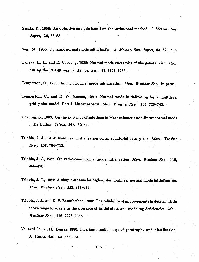
Sasaki, Y., 1958: An objective analysis based on the variational method. J. Meteor. Soc.

Japan, 36, 77-88.

Sugi, M., 1986: Dynamic normal mode initialization. J. Meteor. Soc. Japan, 64, 623-636.

Tanaka, H. L., and E. C. Kung, 1988: Normal mode energetics of the general circulation

during the FGGE year. J. Atmos. Sci., 45, 3723-3736.

Temperton, C., 1988: Implicit normal mode initialization. Mon. Weather Rev., in press.

Temperton, C., and D. Williamson, 1981: Normal mode initialization for a multilevel

grid-point model, Part I: Linear aspects. Mon. Weather Rev., 109, 729-743.

Thaning, L., 1983: On the existence of solutions to Machenhauer's non-linear normal mode

initialization. Tellus, 36A, 30-41.

Tribbia, J. J., 1979: Nonlinear initialization on an equatorial beta-plane. Mon. Weather

Rev., 107, 704-713.

Tribbia, J. J., 1982: On variational normal mode initialization. Mon. Weather Rev., 110,

455-470.

Tribbia, J. J., 1984: A simple scheme for high-order nonlinear normal mode initialization.

Mon. Weather Rev., 112, 278-284.

Tribbia, J. J., and D. P. Baumhefner, 1988: The reliability of improvements in deterministic

short-range forecasts in the presence of initial state and modeling deficiencies. Mon.

Weather Rev., 116, 2276-2288.

Vautard, R., and B. Legras, 1986: Invariant manifolds, quasi-geostrophy, and initialization.

J. Atmos. Sci., 43, 565-584.

135

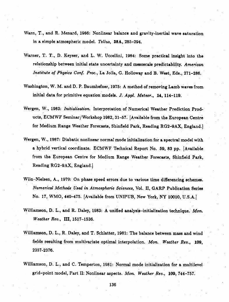
Warn, T., and R. Menard, 1986: Nonlinear balance and gravity-inertial wave saturation

in a simple atmospheric model. Tellus, 38A, 285-294.

Warner, T. T., D. Keyser, and L. W. Uccellini, 1984: Some practical insight into the

relationship between initial state uncertainty and mesoscale predictability. American

Institute of Physics Conf. Proc., La Jolla, G. Holloway and B. West, Eds., 271-286.

Washington, W. M. and D. P. Baumhefner, 1975: A method of removing Lamb waves from

initial data for primitive equation models. J. Appl. Meteor., 14, 114-119.

Wergen, W., 1983: Initialisation. Interpretation of Numerical Weather Prediction Prod-

ucts, ECMWF Seminar/Workshop 1982, 31-57. [Available from the European Centre

for Medium Range Weather Forecasts, Shinfield Park, Reading RG2-9AX, England.]

Wergen, W., 1987: Diabatic nonlinear normal mode initialization for a spectral model with

a hybrid vertical coordinate. ECMWF Technical Report No. 59, 83 pp. [Available

from the European Centre for Medium Range Weather Forecasts, Shinfield Park,

Reading RG2-9AX, England.]

Wiin-Nielsen, A., 1979: On phase speed errors due to various time differencing schemes.

Numerical Methods Used in Atmospheric Sciences, Vol. II, GARP Publication Series

No. 17, WMO, 440-475. [Available from UNIPUB, New York, NY 10010, U.S.A.]

Williamson, D. L., and R. Daley, 1983: A unified analysis-initialization technique. Mon.

Weather Rev., III, 1517-1536.

Williamson, D. L., R. Daley, and T. Schlatter, 1981: The balance between mass and wind

fields resulting from multivariate optimal interpolation. Mon. Weather Rev., 109,

2357-2376.

Williamson, D. L., and C. Temperton, 1981: Normal mode initialization for a multilevel

grid-point model, Part II: Nonlinear aspects. Mon. Weather Rev., 109, 744-757.

136

Williamson, D. L., J. T. Kiehl, V. Ramanathan, R. E. Dickinson, and J.J. Hack, 1987:Description of NCAR Community Climate Model (CCM1) NCAR Technical Note

NCAR/TN-285+STR, 112 pp. [Available from the National Center for Atmospheric

Research, P.O. Box 3000, Boulder, CO 80307, U.S.A.]

137