the vehicle engine cooling system simulation

400 Commonwealth Drive, Warrendale, PA 15096-0001 U.S.A. Tel: (724) 776-4841 Fax: (724) 776-5760

SAE TECHNICALPAPER SERIES 1999-01-0240

The Vehicle Engine Cooling System SimulationPart 1 - Model Development

Oner Arici, John H. Johnson and Ajey J. KulkarniMichigan Technological University

International Congress and ExpositionDetroit, Michigan

March 1-4, 1999

Downloaded from SAE International by Automotive Research Association of India, Friday, August 01, 2014

The appearance of this ISSN code at the bottom of this page indicates SAE’s consent that copies of thepaper may be made for personal or internal use of specific clients. This consent is given on the condition,however, that the copier pay a $7.00 per article copy fee through the Copyright Clearance Center, Inc.Operations Center, 222 Rosewood Drive, Danvers, MA 01923 for copying beyond that permitted by Sec-tions 107 or 108 of the U.S. Copyright Law. This consent does not extend to other kinds of copying such ascopying for general distribution, for advertising or promotional purposes, for creating new collective works,or for resale.

SAE routinely stocks printed papers for a period of three years following date of publication. Direct yourorders to SAE Customer Sales and Satisfaction Department.

Quantity reprint rates can be obtained from the Customer Sales and Satisfaction Department.

To request permission to reprint a technical paper or permission to use copyrighted SAE publications inother works, contact the SAE Publications Group.

No part of this publication may be reproduced in any form, in an electronic retrieval system or otherwise, without the prior writtenpermission of the publisher.

ISSN 0148-7191Copyright 1999 Society of Automotive Engineers, Inc.

Positions and opinions advanced in this paper are those of the author(s) and not necessarily those of SAE. The author is solelyresponsible for the content of the paper. A process is available by which discussions will be printed with the paper if it is published inSAE Transactions. For permission to publish this paper in full or in part, contact the SAE Publications Group.

Persons wishing to submit papers to be considered for presentation or publication through SAE should send the manuscript or a 300word abstract of a proposed manuscript to: Secretary, Engineering Meetings Board, SAE.

Printed in USA

All SAE papers, standards, and selectedbooks are abstracted and indexed in theGlobal Mobility Database


1

1999-01-0240

The Vehicle Engine Cooling System SimulationPart 1 - Model Development

Oner Arici, John H. Johnson and Ajey J. KulkarniMichigan Technological University

Copyright © 1999 Society of Automotive Engineers, Inc.

ABSTRACT

The Vehicle Engine Cooling System Simulation (VECSS)computer code has been developed at the MichiganTechnological University to simulate the thermalresponse of the cooling system of an on-highway heavyduty diesel powered truck under steady and transientoperation. This code includes an engine cycle analysisprogram along with various components for the four mainfluid circuits for cooling air, cooling water, cooling oil, andintake air, all evaluated simultaneously. The code predictsthe operation of the response of the cooling circuit, oil cir-cuit, and the engine compartment air flow when theVECSS is operated using driving cycle data of vehiclespeed, engine speed, and fuel flow rate for a given ambi-ent temperature, pressure and relative humidity.

The one-dimensional, transient, compressible ram air/engine compartment cooling air-flow model was incorpo-rated into the VECSS to enhance the accuracy and thereliability of the cooling air flow rate, temperature, andpressure variation predictions for the ram air/engine com-partment air with improved predictions of the perfor-mance characteristics of the fan, radiator, charge aircooler (CAC), condenser, and the effect of system instal-lation variables. A one-dimensional, unsteady engineheat transfer model was added to calculate the engineliner, head, and piston surface temperatures. The heattransfer model was validated with Detroit Diesel Corpora-tion’s (DDC) steady state engine data. The single passcross flow radiator mathematical model which accuratelypredicts the coolant and air outlet temperatures given theinlet flow and temperature conditions was also added.The model was validated with Behr McCord’s steadystate heat rejection data and agreement between thedata and the model were within 2%. Each of the basiccomponents of the cooling circuit was analyzed individu-ally and modeled and the model predicted results werecompared with the corresponding steady-state experi-mental data. The oil circuit was modeled to represent theconfiguration for the DDC Series 60 engine. New flowand power characteristics for the oil pump were used andmodels for the oil filter, regulator, and oil thermostat weredeveloped. The oil cooler mathematical model was vali-

dated with experimental data from DDC. For the first time,transient pipe lines were introduced in the VECSS pro-gram from the turbocharger to the CAC and from theCAC to the engine air intake manifold. A lag due to inertiain the turbocharger compressor rotor speed was alsointroduced.

INTRODUCTION

For many years, cooling system design was concernedonly with providing sufficient cooling at maximum engineoutput conditions at the worst vehicle operating condi-tions (low vehicle speed and high ambient temperature).This approach results in not achieving the best fuel econ-omy that would be possible with improved design. Withdemands of increased fuel economy, longer engine life,and reduced emissions, greater control of engine perfor-mance is necessary since optimal engine performancecannot be maintained when overcooling occurs.

Ideally, engine cooling is undesirable from the thermody-namic point of view. If the heat transfer rates from the gasto metal could be reduced, then more power could beproduced at a particular fuel flow rate, i.e. the thermalefficiency of the engine would increase. The other majorand probably most important aspect of reducing heattransfer is that there is less heat to remove out of the radi-ator. However, in practice, due to metallurgical con-straints, the conventional engine metals can withstandonly a certain maximum temperature level. At thesehigher temperatures, the fatigue stresses induced in themetal under cyclic loading increase. Engine oil also losesits lubricating qualities when temperatures exceed 177°C(350°F) and, as a result, excessive engine wear occurs.Thus, from a practical viewpoint, engine cooling isextremely necessary for good engine reliability and dura-bility with a compromise of the thermal efficiency. An opti-mum system should offer the following advantages:

1. Increase in coolant, oil, and engine metal tempera-tures during cold start or low ambient temperaturesand light route load conditions.

2. Sufficient cooling of the oil and the engine metal tem-peratures under uphill and full load conditions.


2

For the development of any technical product, one canadvance in two ways. The physical processes within theproduct can be mathematically modeled to accuratelydefine its performance and one can also develop theproduct by laboratory test work. Each of these methodshave their individual advantages. But with the advent ofhigh speed computers, which help in solving the complexsystem of differential equations, the former has thepotential to be lower cost and less time consuming. Incontrast to the experimental approach, a simulationmodel helps the designer to analyze various configura-tions of the system. Simulation of the cooling system fordiesel trucks is one such area where a number of com-puter programs have been developed. The simulationprogram should have the following features:

• Have a systematic structure such that individual com-ponent models can be added to an existing system ormodified to conduct parametric studies.

• Identify key parameters affecting system perfor-mance.

• Help to minimize the hardware tests by establishingthe most important variables to be measured whenexperimentally studying the performance of the sys-tem being modeled for cost benefits and time effi-ciency.

Such a program would provide the designer with an inex-pensive and effective design and analysis tool for design,development, and optimization of the vehicle engine cool-ing system over a wide range of operating conditions. Itwould also enable the designer to analyze various config-urations easily and efficiently for better understanding ofthe operation of modern cooling systems. The VehicleEngine Cooling System Simulation (VECSS) was firstdeveloped at Michigan Technological University in 1982to simulate the thermal response of an on-highwayheavy-duty diesel powered truck under steady state andtransient operation [1]. The VECSS has been developedand validated with experimental data to date using a sys-tem of cooling circuit components in a Freightliner truck[5]. Future research will focus on using the VECSS inparametric and design studies of cooling systems.

OBJECTIVES

The goal of this paper is to present the latest improve-ments to the Vehicle Engine Cooling System Simulationwhich involves incorporating Chang’s one-dimensional,transient, compressible ram air/engine compartment air-flow model [2]. The existing program used a very simplis-tic and elementary airflow model to predict the air flowrate across the radiator-shroud-fan system. Also, theexisting model did not have the flexibility to change thesystem physical dimensional characteristics. The pre-dicted air flow rate by the existing program was found tobe much higher than the experimental data supplied byKysor cooling systems [3]. In addition, the existingVECSS version was not updated by Mohan [4] to incor-porate the DDC coolant and oil circuit configuration. The

VECSS program had not been validated recently withgood steady-state and transient field data. Kysor coolingsystems and Detroit Diesel Corporation collaborated inMay-June 1996 to gather extensive data that would beused in validation of the updated VECSS. Kysor of Cadil-lac used a Hewlett Packard (HP) data acquisition systemand DDC used the Detroit Diesel Electronic Controls -Electronic Control Module (DDEC-ECM) to record dataon a Freightliner FLD 120 truck with a 12.7 L Series 60engine, a Behr McCord radiator, an Allied Signal charge-air cooler, and Kysor DST variable speed fan clutch. Thevalidation data are compared to VECSS data in the com-panion Part 2 paper by Arici et al [5].

An upgraded description of all the simulated componentsof the VECSS program will be discussed first. Thisinvolves changes for the components in the three circuits,namely the circuits for the coolant, oil, and intake air tothe engine. The mathematical formulation of the modelsfor the different components of the cooling system, thevalidation of each model and explanation of the physicalprocesses occurring in them are provided. The develop-ment of one-dimensional, unsteady, engine heat transfermodel, which calculates the engine liner, head and sur-face temperatures at varying load and speed is dis-cussed.

The paper details the incorporation of the one-dimen-sional, compressible, transient airflow model developedby Chang [2]. It describes how this work enhanced theaccuracy and reliability of the airflow, temperature, andpressure variation predictions of the VECSS programwith more realistic performance characteristics for fan,shroud, radiator, charge air cooler, condenser, and grill. Itdetails how the end user can design a new configurationfor the cooling airflow system and study variables relatedto the system installation.

REVIEW OF PAST WORK

Ursini, et al [1] and Chiang et al [6] originally developedthe Vehicle Engine Cooling System Simulation (VECSS)at Michigan Technological University in 1982. This com-puter program modeled the International Harvester COE-9670, on-highway heavy-duty diesel powered truck withthe Cummins NTC-350 Big Cam II aftercooled dieselengine. Ursini validated the VECSS by correlating thepredicted Air-To-Boil (ATB) number with experimentaldata by using several empirical relationships for theengine and oil system models in order to obtain satisfac-tory results at the full load, rated speed, and peak torqueoperation [7]. Savonen [8] continued Ursini’s work byimproving the radiator and oil system models whichincreased the capabilities of the computer simulation pro-gram to cover vehicle operation over a wide range underextreme ambient temperature conditions. The finite differ-ence formulation to solve the coupled, transient govern-ing equations gave a more representative simulation ofthe radiator performance during vehicle warm-up and lowradiator coolant flow. The program’s capabilities werealso expanded to allow the use of 50/50 ethylene glycol


3

as the engine coolant. These developments allowedSavonen to conduct parametric studies of the thermalcontrol devices at extreme ambient and truck operatingconditions [9]. Chellaiah [10], as a further enhancementto the development of transient truck cooling system sim-ulation, modeled a two pass cross-counterflow radiatorused in low flow cooling systems. He validated the modelwith field data collected by the Cummins Engine Co., dur-ing an on-road test run of a Peterbilt truck fitted with theCummins Big Cam IV aftercooled engine with a low flowcooling system. Although the simulation results followedthe general data trends, amplitude deviations were some-times excessive, and, in addition, the predicted trendswere, in some cases, different from the actual datatrends. Chiang attributed these discrepancies to deficien-cies in the coolant thermostat modeling scheme [11]. Xu[12,13] modified the VECSS to simulate a microproces-sor-sensor-type controlled cooling system. The obviousgoals were to increase thermal efficiency, reduce fanengagement time, reduce power to the water pump, andincrease engine temperature for cold start and low ambi-ent temperature as opposed to a wax-sensor-actuatortype controlled cooling system. From this study, the hard-ware and software for a prototype computer controlledcooling system was demonstrated in an engine dyna-mometer test. Keller [14] continued Chellaiah’s work byimproving the model of the thermal control devices. Heworked on the coolant thermostat model and also built aradiator shutter/shutterstat model. His main contributionwas validating the VECSS by comparing the predictedATB numbers to measured ATB numbers at three differ-ent engine speeds [15]. The predicted ATB numbersmatched well at an engine speed of 1900 rpm, but thecorrelation became poorer at a lower engine speed of1300 rpm. The predicted ATB number was overestimatedby 1.7°C (3°F) at 1300 rpm. Chapman [16] determinedthat the deficiency in the VECSS was the engine model.The original model used by previous researchers was toosimplistic and empirical to correlate to experimental dataover a wide range of engine loads and speeds. Heimproved the engine model by incorporating an idealizedcycle analysis method which predicted a load and speeddependent heat transfer coefficient, in-cylinder cycleaverage gas temperature, and engine coolant tempera-ture rise [17]. He made modifications to the turbochargerand coolant pump model. He also incorporated an airconditioning model. He validated this version of theVECSS by comparing the predicted and actual tempera-ture data from ATB and transient tests. Hovin [18] devel-oped a microprocessor controlled lubricating oil coolingsystem. In addition, the standard thermostats werereplaced by controllable valves, and the fan and shuttersystems were controlled by actuators. This VECSS wasalso capable of setting the coolant and air flow ratesbased on the dynamics of the system and the currentoperating conditions [19]. Chang [2] developed a one-dimensional, transient, compressible airflow model topredict the airflow behavior for truck engine cooling sys-tems. After development of this model, he calibrated andvalidated it to conduct parametric studies to investigate

the effects of operating and ambient conditions on cool-ing airflow [20]. He also studied the effects of installationparameters on the air circuit and heat rejection. Thismodel was separate from the VECSS program. In 1993,the main frame version of the VECSS was converted to aPC version. Mohan [4] continued the development of theexisting Vehicle Engine Cooling System Simulation(VECSS) version by incorporating a new engine cycleanalysis model simulating the Detroit Diesel Corpora-tion’s (DDC) Series 60 engine to replace the existingengine model. He modeled the turbocharged direct-injec-tion diesel engine using “cycle analysis” concept, whichgave good results at rated speed and load and even atpart loads unlike the previous engine model. Theenhanced engine model was extensively validatedagainst steady-state data supplied by DDC [21]. He alsoreplaced the air-to-water aftercooler model in the earlierVECSS with Allied Signal’s air-to-air charge air coolermodel.

VECSS PROGRAM REVIEW

The current code of the Vehicle Engine Cooling SystemSimulation (VECSS) has been run on a Pentium II / 300MHz with a 128 MB RAM PC running on DOS 6.22 andWindows NT. The Fortran compiler used is the LaheyF77L3 EM/32 Version 7.0. The latest version 8.1 of theVECSS is capable of predicting real-time thermal perfor-mance of a diesel engine cooling system during steadystate and over-the-road transient operation. The com-puter model is built of various subroutines each effec-tively representing a different component of the coolingsystem. The model, currently, contains various subrou-tines which simulate the engine, radiator, charge aircooler (CAC), fan, ram air/engine compartment airflowcircuit, turbocharger, coolant circuit, cab heater, thermalcontrol devices (radiator/bypass thermostat, fan control,oil thermostat etc.), oil circuit, regulator valve, oil cooler,and oil filter, as shown Figure 2. Most of these majorcomponents are modeled mathematically with a transientapproach to predict and represent the steady state aswell as the transient operation. All the physical dimen-sions for the components are provided by means of sev-eral input files. This gives flexibility within the model sothat any component can be replaced with a differentmodel with different characteristics. This systematicapproach makes possible future improvements, addi-tions, and modifications. For the software to run, threemain run-time data have to be provided; these are theengine speed, the engine load given by the fuel flow rateand the vehicle speed as shown in Figure 1. The ambientair, temperature, pressure, relative humidity and thevelocity (wind speed) is also provided as input datathrough an input file and is maintained at a constantvalue throughout the simulation.

ENGINE MODEL – The engine model is a critical compo-nent of the VECSS software, since energy rejection to thecoolant and the oil comes from the engine. The six cylin-der diesel engine was modeled by assuming that all the


4

cylinders operated at approximately the same operatingconditions making it possible to mathematically modelone engine cylinder and extend the results to the remain-ing cylinders. The engine cycle analysis simulation mod-eling and its validation was done by Mohan [4,21].

Figure 1. Vehicle-Engine-Cooling System in Freightliner FLD 120 truck.

Combustion was modeled as a single-zone heat releaseprocess. The gas exchange process uses a one-dimen-sional quasi-steady compressible flow model. The heattransfer model uses modified Annand’s correlation forcalculating convection heat transfer. The radiative heattransfer was calculated based on flame temperature. Thefrictional model converts indicated quantities (power, indi-cated specific fuel consumption (isfc), etc.) to the corre-sponding brake quantities. A steady-state turbochargermodel, manifold heat transfer, and pressure losses werealso included in the simulation. Finally, the engine modelcalculates the surface temperatures and metal massaverage temperatures for piston, cylinder head and liner,and exit temperatures of coolant and oil. This one-dimen-sional unsteady heat transfer simulation model to calcu-late the above mentioned temperatures developed byMohan [4] was improved and is discussed later.

DESCRIPTION OF INDIVIDUAL COMPONENTS – Thewhole VECSS program can be divided basically into fourmain circuits, Figure 2.

1. Coolant circuit comprising of the coolant pump, cabheater, oil cooler, engine, radiator/bypass thermostat,fan actuator, and the radiator.

2. Oil circuit comprising the oil pump, oil filter, oil ther-mostat, oil cooler, regulator valve, oil gallery, mainbearing cooling circuit, crank bearing cooling circuit,piston cooling circuit, accessories cooling circuit, andthe oil sump.

3. Ram air / engine compartment circuit comprising ofthe grill, charge air cooler, condenser, radiator,shroud, fan, and the branching in the compartmentaround the engine.

4. Intake air circuit comprising of the turbocharger,charge air cooler, engine, and the exhaust.

Figure 2. Complete schematic of Vehicle Engine Cooling System

COOLANT CIRCUIT – The coolant system consists ofthe following major components: coolant pump, cabheater, engine, thermostat, fan actuator, and radiator.The coolant circuit which was used in the previous ver-sion of the VECSS was a low flow coolant system[1,6,7,8]. However, when the air-to-air charge air coolerwas introduced, the truck manufacturers switched to theconventional radiator for increased operating tempera-tures and hence increased thermal efficiency [4]. Since,the present truck under study has a conventional radiatorwith air-to-air charge air cooler, necessary modificationswere required to be made to the coolant circuit, radiator,and aftercooler models in the existing VECSS. The cen-trifugal pump is used to circulate the engine coolant.Pressurized coolant from the pump is forced through theoil cooler and the engine. Heat rejection from the engineis the main source of energy to the coolant. The fullblocking-type thermostat is used to control the flow ofcoolant through the radiator, providing fast engine warm-up and regulating coolant temperature. When starting acold engine or when coolant is below operating tempera-ture, the closed thermostat directs all the coolant throughthe bypass to the pump. When the thermostat openingtemperature is reached, coolant flow is divided betweenthe radiator and the bypass tube. When the thermostat isfully open, 70% of the coolant flows through the radiatorand the remaining 30% flows through the bypass. Thecoolant circuit schematic provided by DDC is shown inFigure 3.

COOLANT PUMP – The coolant pump circulates thecoolant through the engine cooling system. The pump isdriven directly off the engine by means of a gear mecha-nism. Data points relating pump flow with engine speedwere supplied by DDC. An equation was developed tocalculate the pump flow as a function of the engine speedusing these data points. The power used by the pump iscalculated by standard pump laws. The coolant pumpwithin the cooling system is assumed to have no effect on

F uel f low rate

E ng ine speedVeh ic le speed

Cylinder Head

Cylinder Block

Thermostat & Shutterstat

Oil Pump

Oil

Co

ole

r Coolant PumpThermostat

Rad

iato

r

Fan

Byp

ass

AIRFLOW

OIL SUMP

CA

C

cab heater


5

fluid temperature. The pumping of a fluid through the sys-tem generates an increase in thermal energy due to fluidfriction (which is dependent upon fluid viscosity and sys-tem pressure). For an engine application, these effectscan be assumed negligible in comparison to the thermalenergy transferred to the coolant from the engine’s com-bustion heat transfer process and frictional effects. Themost important parameter describing the pump is therate at which the coolant is pumped. For these reasons,no attempt was made to theoretically model pump perfor-mance.

Figure 3. Coolant flow schematic for DDC series 60 engine

CAB ENVIRONMENT MODEL – The cab environmentmodel is included in the VECSS since the cab heater unitin the coolant circuit removes energy from the system.The cab environment is not the main component of thecooling system, but the cab comfort and performance ofthe cooling system are coupled through the cab heater.The mathematical models of the cab environmentdescribed here were included in the new version ofVECSS without revision. The detailed model was devel-oped by Ursini [1] and are for the International HarvesterCOE - 9670 truck.

The cab environment control system consists of the cabheater unit with three position blower and insulated cabwalls. Cab blower setting is dependent upon driver prefer-ences. A simple logic used to simulate the driver’sresponse to cab air temperature determines blower set-ting and consequently cab comfort levels. This assumesthat the desirable temperature inside the cab at all ambi-ent temperatures is 21 to 27°C (70 to 80°F). Hence, theblower settings are made to fluctuate accordingly toachieve this comfort temperature zone. The followingflowchart in Figure 4 shows blower settings at variouscomfort temperatures:

Figure 4. Cab Blower Setting Flowchart

After determining the flow rate through the blower, theinlet air temperature to the cab heater or the temperatureout of the blower is determined based on the percentageof fresh air allowed to mix with recirculated air. The inletdoor position will allow for about 15 - 100% of fresh airoperation. A certain percentage of fresh air is alwaysadmitted into the cab to reduce irritating smoke and dusteffects. The inlet door may be controlled by a vacuumactuator or by gravity. The percentage of fresh air varieswith vehicle speed for gravity operated doors. As thevehicle speed increases, the amount of recirculation airdecreases. For the analysis here, 50% of fresh air and50% of recirculated air was assumed to exist for all vehi-cle speeds since the actual air inlet versus the vehiclespeed maps are not available.

Once, the inlet air temperature and the flow are estab-lished, this mass of air flows over a blend door. The blenddoor can be used to vary the percentage of inlet air that isdirected through the cab heater core. Adjusting blenddoor position regulates heater effects on the cab air tem-perature without adjusting the blower speed. The presentVECSS assumes that the blend door is maintained in thefull open position directing all inlet air through the heater.

The cab heater model is a coolant to air finned heatexchanger. The heater is operational only when ambienttemperatures are below specified cab comfort levels.

To evaluate the average cab air temperature, it is neces-sary to know the heat energy which is absorbed by thecab walls and/or interior, the energy which is dissipatedthrough the walls and/or the energy lost by infiltration ofthe ambient air (leakage of ambient air into the cab) inaddition to the heat energy entering the cab from theheater.

In order to calculate cab surface heat rejection, the cab isdivided into six different wall types, namely, the frontpanel, the windshield, the side panels (the doors), toppanel, rear panel and floorboard. The overall heat trans-fer coefficients must be evaluated for each of these walls.

The thermal resistivity value or R value is determined foreach wall. In case where the wall composition varies, thevalue is averaged over the length of the panel. Surfacearea and panel length parallel to air flow is also deter-mined for each wall.

C y lind er H ead

C y lind er B lo ck

O il co o le r

Rad

iato

r

C oo lan t pu m p

T herm os ta t

Coo

lant

fan

B y pass tub e

C o o lan t pa th

C ab

Tcab < 2 1 .1oC (7 0oF ) 0.189 m3/s (400 CFM)

No

YesYes

2 1 .1oC (7 0oF )< Tcab < 2 3 .9oC (7 5oF ) 0.142 m3/s (300 CFM)

No

Yes

2 3 .9oC (7 5oF )< Tcab < 2 6 .7oC (8 0oF ) 0.083 m3/s (175 CFM)

No

Yes

Tcab > 2 6 .7oC (8 0oF ) 0 m3/s (0 CFM)

Yes


6

Internal convection coefficients are assumed to be gov-erned by natural convection. Use of Grashoff numberallows determination of internal convection terms foreach wall based on cab-ambient temperature difference.

THERMOSTAT MODELING – Thermostats are tempera-ture - sensitive flow control valves. They are used to con-trol the flow of coolant through the radiator and maintainthe temperature within a specified range in the coolantcircuit. Their operation is in response to the temperaturessensed by the wax sensor.

The themostat sensor begins to open when the liquid intowhich it is immersed reaches the thermostat start-to-open temperature (also called the thermostat activationtemperature), directing some liquid to flow along the newpath. If the temperature continues to rise, the valve fur-ther opens until its full open temperature is reached.When this happens, maximum flow is directed throughthe radiator in the cooling system. As the system coolsdown, the reverse action takes place.

The most common type of thermostat used is solid/liquidphase wax actuator. The brass housing (cup) in thesekind of thermostats is filled with a heat expansive waxmaterial that is compounded to provide accurate, repeat-able temperature response. The wax is sealed within thecup by an elastomeric sleeve. The sleeve envelops a pol-ished stainless steel piston with tapered end. A seal andbrass cover completes the sealing of the unit.

The brass cup is in the path of the liquid flow. Heat is con-ducted through the walls of the cup to the wax. As thewax within the brass cup reaches its special compoundedthermostat, it melts and expands, displacing the piston bysqueezing the sleeve. The piston is in turn moved by thesleeve and the valve opens. As the temperature drops,the wax contracts allowing the piston to return. Operationof the plunger can be controlled mechanically or by vary-ing the melting point temperature of the wax material (thiscan be achieved by adding varying amounts of copperfiller).

Thus to appropriately model the thermostat, the differentprocesses happening within the thermostat have to care-fully understood. The different processes that take placein succession before the thermostat is actuated are:

• Heat transfer by convection from the hot liquid to theouter surface of the brass cup (in contact with thecoolant).

• Heat transfer by convection through the cup to itsinner surface.

• Heat transfer by convection to and through the wax

• Melting and increase in volume of wax.

• Movement of the piston and finally the actuation ofthe valve.

A rigorous model should consider each of these pro-cesses. But, for a system modeling approach like thiscooling system simulation, such a complicated andinvolved model is not necessary. So, a different method is

used which takes into consideration a characteristic timelag associated with the thermostat just like any mechani-cal control device would have. There is a definite timegap between the instant the thermostat senses the tem-perature, and the instant the actuator starts to function.The time difference between the response and the stimu-lus is called the ‘time delay’. In the case of a thermostatthis time delay is the sum of the mechanical and the ther-mal lags. It takes sometime for the wax to reach its melt-ing point after the cup has reached that temperature. Thisis called the thermal delay. Again, the actuators do notact instantaneously. This lag is called the mechanicaldelay.

In the present cooling system, the flow to the radiator iscontrolled using a single thermostat. This model consid-ers that the sensor temperature is governed by the linear,first order, ordinary differential equation [8,22]:

(1)

where, THT is the temperature of the thermostat housing,TST temperature of the sensor, MC thermal capacity ofthe housing, U overall heat transfer coefficient, A areaassociated with U, and t time.

The ratio of UA/MC is defined as the time constant of thethermostat. The value of the time constant is determinedusing experimental data [10]. The sensor temperaturecan be found out using the above equation, given thehousing temperature which is equal to the coolant tem-perature flowing through the thermostat.

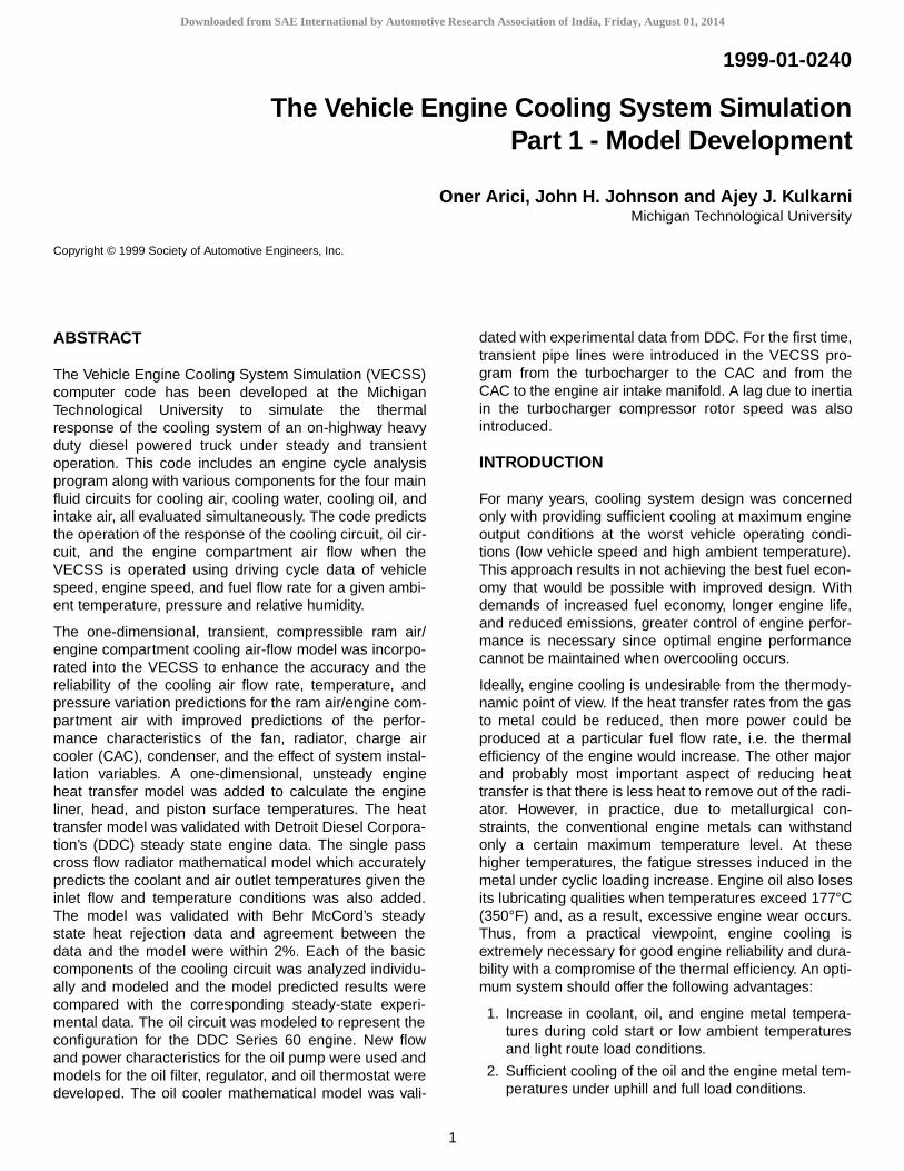
After the sensor temperature is calculated, and knowingthe operating characteristics of the thermostat, the lift ofthe radiator thermostat is calculated using Lagrangeinterpolation. Thus for any operating condition, the flowthrough the radiator is determined using the flow factorscalculated based on the lift. For the specific thermostatused for analysis, the activation temperature is 87.8°C(190°F). Below this all the coolant flows through thebypass and the thermostat is completely closed. Whenthe sensor temperature reaches to 96.1°C (205°F) thethermostat reaches its maximum opening which allows70% of the coolant to flow through the radiator. In theoperating range from 87.8°C (190°F) to 96.1°C (205°F),the thermostat is continuously opening and closing. Thethermostat never completely opens such that all coolantflows through radiator [29].

Due to the repetitive opening and closing of the thermo-stat, a hysteresis loss is incurred, i.e., the lift of the ther-mostat valve or the movement of the plunger will bedifferent when the thermostat is opening and closing forthe same sensor temperature. Thus, there are two, ther-mostat lift vs. sensor temperature curves. One for open-ing and one for closing of the thermostat. One importantpoint to be noted is that the thermostat will not fully closeuntil the liquid temperature is below the activation tem-perature. A hysteresis lag of 1.7°C (3°F) is built in thethermostat model, as shown in Figure 5. The programafter detecting the mode of operation, checks if the ther-

UA( ) THT TST–( )⋅ MC( )td

d TST( )⋅=


7

mostat is opening or closing and accordingly incorpo-rates the hysteresis lag.

Figure 5. Coolant thermostat characteristic curve

RADIATOR MODELING – The radiator is the mostimportant heat exchanger in the engine cooling systemas it transfers the majority of the thermal energy from thecoolant to the surrounding air. Hence, it is extremely cru-cial to model the radiator accurately for effective function-ing of the coolant circuit.

The radiator is a liquid to air heat exchanger. It experi-ences a large variation in coolant inlet condition and flowrate. The radiator flow may be small or large or it may beextremely low and there will be no flow when the engineis shut down or the thermostat is completely closed. Theflow depends both on the radiator thermostat position aswell as the performance of the coolant pump. The opera-tion of the thermostat is explained in the previous section.The coolant flows through the radiator, only when thecoolant temperature reaches the thermostat control tem-perature. Therefore, the radiator flow varies from 0 gal/min (when the thermostat is fully closed) to 70 gal/min(when thermostat is 70% open and the total coolantpump flow is 100 gal/min). Hot coolant enters the radia-tor, where it is cooled by ram (ambient) air. Ram air flowis controlled by the shutters (if the truck is so equipped)located at the back of the radiator and in front of the fan.Depending on the amount of cooling required, the shut-ters are open or closed.

The coolant exiting the radiator then mixes with the cool-ant from the bypass and the coolant from the cab heater,and is then pumped to other parts of the coolant circuit(Figure 2). The shutters were not used in this work forcoolant temperature control since the Freightliner truckused to collect data was not so equipped.

The primary purpose of the radiator model is the determi-nation of the radiator outlet coolant temperature. In gen-eral, there are three ways to analyze the performance ofa heat exchanger [11]. They are:

1. The Log-Mean Temperature Differential approach(LMTD)

2. The Net Transfer Units method (NTU)

3. Numerical method

The main drawback of the first two methods is that theyare applicable only for steady state conditions. For ana-lyzing the transient response of a heat exchangers, atime delay function coupled with the NTU method wasused for initial versions of VECSS. This approach needsa closed form expression for effectiveness. Also, theresults were not very satisfactory, mainly during thewarm-up period [1,6]. Later, a two pass cross counterflowradiator was developed for the low flow cooling systemusing the Euler explicit numerical scheme [11,12]. Thisscheme was insufficient because the results had a largetruncation error.

The new conventional radiator modeled represents theBehr McCord’s radiator (Model 405-16366-001) used inthe validation tests. The radiator is a single pass crossflow type heat exchanger. Hot coolant from the enginehead enters the radiator from the top side, flows throughthe single pass tubes and exits through the bottom of theradiator. The ambient air enters through the front side ofthe radiator, picks up heat from the first row of coolanttubes, the second row and finally the third row of tubes.Thus the coolant and the air enter the radiator from differ-ent directions having crossflows. The radiator tubes arefitted with continuous serpentine fins to increase the heattransfer on the air side. The coolant and air do not mix. Athermal mixing of the coolant takes place at the top andthe bottom of the radiator. Thus the temperature of thecoolant entering each tube from the top tank is the sameand it varies along the tube till it reaches the bottom tank.On the other hand, since the air gets heated up as itpasses over the first row of tubes, the air temperatureentering is higher for the second row and then still higherfor the third. Mixing of the air is assumed between tuberows and hence the inlet air temperature for all tubes in aparticular row is the same.

The coolant entry for all tubes is located at the top of theradiator. Therefore, the coolant flow rate through eachtube is the same. Airflow rate across the radiator is evalu-ated from the ram air / engine compartment airflow modelwhich is explained later in the paper.

To obtain the dynamic response of the radiator by meansof the Runge-Kutta fourth order numerical scheme, thefollowing assumptions were made in the analysis:

• Negligible axial conduction in the coolant.

• There is no heat generation within the radiator.

• Conduction through the wall is negligible.

• Properties of the tube like the specific heat, density,and thermal conductivity remain constant at all tem-peratures.

• Uniform inlet air temperature and velocity along thefull length of the tube.


8

• There is complete thermal mixing of the coolant andair at the inlet and outlet of each tube row.

• No mixing of the coolant takes place within the tube.

• The fluid velocity is the same at all points and is influ-enced only by the changes in the flow rates.

In the radiator, the two fluids, hot coolant and the ambientair, are separated by the tube wall. Heat transfer takesplace by two modes, conduction and convection. Heat istransferred from the coolant to the wall by: (1) forced con-vection, (2) by radial conduction from the inside of thewall to the outer surface, and (3) from the outer surface ofthe tube to the ambient air by forced convection. Thesmall thickness of the tube makes the conductive resis-tance of the tube wall negligible. Therefore, the dominantmode of heat transfer is forced convection. Any techniqueused must be capable of predicting the temperature ofthe coolant, air, and metal at different times and at differ-ent locations under varied operating conditions.Although, the coolant and the air temperature are ofprime significance, it is advantageous from a design pointof view to know the metal temperatures also. This helpsthe designer to know the temperature distribution in thebody of the radiator for the necessary analysis of thethermal stress effects.

The radiator has 3 rows with 47 tubes per row, 32 deg.louvered fins and a fin density of 14 fins per inch. Tomodel the radiator, each of the three rows where mod-eled separately because the inlet air temperature was dif-ferent for each one. In a particular row, only one tube wasmodeled and the analysis was extended to the other 46tubes. Each tube was divided into 10 segments. Theapplication of the First Law of Thermodynamics for thecoolant, metal and the air to each segment resulted in aset of three coupled differential equations:

(2)

(3)

(4)

where, mCp is thermal capacity, h heat transfer coeffi-cient, A surface area for heat transfer, T temperature, andt time. The subscripts are, m for metal, c coolant, a air, iinlet, and o outlet.

Before attempting to solve the above coupled differentialequations all the physical dimension like the area, vol-ume, and the internal and external heat transfer coeffi-cients must be determined. The internal heat transfercoefficient depends only on the coolant flow rate and isunaffected by the air flow rate. The rate of heat removedby air from the coolant depends directly on the air flowrate, and only indirectly on the internal heat transfer coef-ficient. Similarly, the external heat transfer coefficientdepends only on the air flow rate and is not influenced bythe coolant flow conditions. Again, the rate of heat

removed from the coolant depends on the coolant flowrate but not on the external heat transfer coefficient.

Having determined the heat transfer coefficients, for aparticular operating condition, all the coefficients in thecoupled differential equations are known. The self start-ing numerical method Runge-Kutta fourth order formulawas used.

The set of equations were solved simultaneously first fornode 1 using the Runge-Kutta fourth order formula. Theinitial condition at t=0 is that the entire core of the radiatorand the air are at ambient temperature. The temperatureof the coolant exiting node 1 is the temperature of thecoolant at entry node 2. Thus the coolant temperature ofeach node was used for analysis of the successive node.A time increment of 1 second was used. The solution didnot converge and in fact was diverging. Hence, smallertime steps were used till the solution converged.

Steady state experimental data obtained from BehrMcCord at three different coolant flow rates of 3.16, 4.42,5.68 L/s (50, 70 and 90 gal/min) and four different air flowrates of 4.06, 5.08, 6.1, and 7.1 m/s for each coolant flowwas used to validate the computer model at differentoperating conditions. The coolant used in this case was50/50 glycol-water. Figure 6 shows the heat rejectionrates for an inlet temperature differences of 50°C (datafor increments of 100°F). The inlet temperature wasassumed to be at 21.1°C (70°F) and the inlet coolanttemperature is at 76.7°C (170°F). As can be seen, themodel predictions were in good agreement with theexperimental data (within 2%).

Figure 6. Radiator heat rejection rate at different coolant flow rates

OIL CIRCUIT – For analysis of the cooling system, astudy of the oil circuit is extremely important as it has adirect effect on the coolant temperatures because thecoolant gains energy from the oil in the oil cooler. Also,the oil system may be considered a cooling system initself with oil as the cooling medium. The heavy duty die-

mCp( )m td

dTm hcAc Tc Tm–( )( ) haAa Tm Ta–( )( )–=

mCp( )c td

dTc mCp( )c

Tc i, Tc o,–( ) hcAc Tc Tm–( )–=

mCp( )a td

dTa mCp( )a Ta i, Ta o,–( ) haAa Ta Tm–( )–=


9

sel engine oil circuit has two purposes. First of all, it isused to lubricate the engine parts to reduce engine wearand bearing load. Secondly, the oil serves as a coolantreducing the temperatures of the piston and bearings.

The original oil system model [1] which utilized an energybalance at the engine cylinder to determine energy allo-cation to the oil for given engine operating conditions wasfound unsatisfactory. Hence, Savonen [8] developed anew model which consisted of an empirical and analyticalformulation. It consists of several component modelswhich predict the significant energy transfer rates withinthe oil system. The model developed by Savonen wasbased on the oil system used for the Cummins NTC-350diesel engine. But, since the predictions here are ana-lyzed for the Freightliner truck with the Detroit DieselSeries 60 engine, the accuracy of the present oil systemmodel depends on the correct representation of theseenergy transfer processes. Figure 7 shows the schematicof the oil system for the DDC Series 60. This can be com-pared with the old oil system [6].

Following were the changes in the oil circuit for which ithad to be remodeled:

• The oil filter position is changed for the DDC engine.

• The regulator valve position is changed.

• The thermostat characteristics used for the Cumminsengine are different than the one used for the DDCengine.

• Characteristics of the oil pump are different.

• Other physical parameters like the bearing dimen-sions, mass and area dimensions of various compo-nents are different.

• Mass of oil in the sump and the sump physical prop-erties are different.

All the required physical dimensions and material proper-ties were supplied by DDC [29]. The oil system consistsof the following major components: oil pump, twin oil filter,oil thermostat, oil cooler, main and connecting rod bear-ing heat rejection, piston cooling heat rejection, and oilsump.

Figure 7. Oil schematic presently used with DDC Series 60 engine

OIL PUMP – The oil pump just like the coolant pump cir-culates the oil through the oil system. This pump too isdriven by the engine, hence its speed varies with theengine speed. A second order polynomial curve fitted tothe experimental data is used to model the oil pump flowrate and the power consumption is calculated using stan-dard pump laws [22]. The oil pump contributes signifi-cantly to the heating of the oil. Hence, the viscousheating of the pump due to pump losses cannot beneglected. Rise in oil pressure and irreversible increaseof the internal energy of the oil occurs at the pump due topump input work. As the oil travels in the system, frictiondissipation causes an increase in the internal energy ofthe oil. Essentially, the power used by the pump eventu-ally turns into internal energy of the oil. Hence, the pumppower calculated using the above equation is used to cal-culate temperature rise in the oil pump.

OIL FILTER – The oil filter is considered to be an addi-tional oil sump because of its size in this system. Incom-ing oil mixes with that contained within the filter todetermine a representative oil filter temperature. Theeffect of oil filter ambient heat loss is considered negligi-ble. An energy balance gives the governing relation forthe oil filter [22].

(5)

Here MCp is heat capacitance of the oil filter, Tf represen-tative temperature of filter oil, filter oil mass flow rate,Cp specific heat of oil, and Tif temperature of oil enteringfilter.

OIL THERMOSTAT – The oil thermostat in the previousVECSS version had a sizeable amount of oil cooler oilflow even when the oil thermostat was in the fully closedposition. With the changed thermostat characteristics forthe new oil system, the thermostat is similar to the cool-ant thermostat. The activation temperature is fixed at104.4°C (220°F) and is fully open at 113.9°C (237°F). A5% leakage is introduced in the thermostat when the oiltemperature is below the activation temperature 100% ofoil flows through the oil cooler when thermostat is fullyopen.

OIL COOLER – The pump oil from the sump passesthrough the filters to the oil cooler. During the warm-upperiod, a small amount of oil flows through the oil coolercorresponding to the thermostat leakage of 5% of thefully open position. During the working of the thermostat,the oil flowing through the oil cooler transfers heat to thecoolant and the cooled oil is directed towards the regula-tor valve.

The oil cooler used with the DDC series 60 engine ismanufactured by Harrison Division of General MotorsCorp. It is a shell and tube type with single pass shell anda double pass tube. The oil flows through the shell andthe coolant flows through the tube.

o il su m p

o il pu m po il su rface

oil f i lters

o il th erm os ta t

o il co o le r

m a in g allery

(o pen s at 2 .9 6 5 b ar)

regu lato r v alv e

(fu lly c lo sed 1 04 .44 -1 05 .5 5 d eg C fu lly o p en 113 .8 9 d eg C )

MCp td

dTf m· Cp Tif Tf–( )=


10

The NTU approach is used to calculate the exit tempera-tures of the two fluids. Knowing the surface areas, thefluid flow rates and calculating the inner and outer heattransfer coefficients, the effectiveness for the oil cooler isevaluated. The correlations used for inner and outer heattransfer coefficients and the procedures are discussed atgreat length in Reference [22]. The existing oil cooler wasaccordingly modified to accurately represent the presentoil cooler and was validated against the experimentalheat transfer data. Table 1 gives the comparison of the oilcooler model predictions with the experimental data giventhe inlet oil and coolant flow and temperature conditions.The model predictions were within 2% of the experimen-tal data for the all the seven conditions.

BEARING HEAT ADDITION – There are basically threemajor sources of oil heating: oil pump internal energyincrease, bearing internal energy increase, and the pis-ton cooling heat addition. The purpose of the bearingmodel is to predict the oil flow to the main and big-endconnecting rod bearings and the energy generation ratesat varying engine operating conditions. The bearingmodel developed by Savonen [8] is relatively simple andis a representative prediction of the mean cyclic bearingperformance [22].

The theory is governed by the theory of hydrodynamiclubrication. Hydrodynamic theory for dynamically loadedjournal bearings (main and con rod bearings) is verycomplex. But, relatively straight forward methods areavailable to determine bearing performance for constantspeeds and constant loads. The classical short bearingtheory described by Ocvirk [23] is used.

Bearing flow can be determined based on two compo-nents:

1. flow associated with the bearing hydrodynamicpumping action.

2. flow due to external pressure feed.

The external pressure feed is necessary to effectivelyand efficiently remove energy from the bearings. This isprovided by the main rifle. The main rifle pressure isdetermined in the VECSS program using experimentalmaps of rifle pressure versus engine speed. Under nor-

mal operating conditions, the rifle pressure is maintainedrelatively constant by the pressure regulator.

The oil flow relations used for the main bearing and thebig-end con rod bearings are:

for main bearing oil flow,

(6)

for big-end con rod bearing oil flow,

(7)

where, is bearing oil volumetric flow rate, Cr bearingradial clearance, D bearing shaft diameter, Ps main rifleoil pressure, ε bearing eccentricity, U rotational speed ofbearing shaft with respect to bearing housing, l axiallength of bearing, d oil supply hole diameter, and µdynamic viscosity of oil.

The first term in both the equations is the pressureinduced flow component. The second term representsthe oil flow due to the hydrodynamic bearing pumpingaction when using the short bearing theory.

After the oil flow to each of these bearings is determined,the second step is to calculate the rise in temperature ofthe oil flow, given the inlet temperature. For this, the rateof frictional work for the oil is calculated and assumingthat the oil carries away all of this energy, the exit temper-ature for the oil is evaluated.

A simple equation adopted from the short bearing theoryto calculate frictional power is:

(8)

where E is the rate of frictional work produced by bear-ing.

Modeling of this complete heat transfer mechanism isavoided in the analysis and since, the generated bearingenergy is assumed to give a rise in the oil temperature,regardless of the path it takes, we can say,

(9)

where, is heat transfer rate to oil from bearing, heat capacitance rate of oil bearing, Tbr2 oil

temperature exiting bearing, Tbr1 oil temperature enter-ing bearing.

One of the significant variables that has to be evaluatedis the bearing eccentricity, ε, a measure of the radial dis-placement of the bearing shaft from the axis of the bear-ing. As the bearing load and, therefore, the bearingeccentricities vary significantly through out the enginecycle, a representative or average load and a corre-sponding eccentricity is chosen for the analysis.

Table 1. Comparison of Oil Cooler Steady State Experimental Data and VECSS Predicted Data

Condition No. 1 2 3 4 5 6 7

Oil flow (L/s) 3.166 1.894 0.632 3.349 2.696 1.985 1.042

Inlet oil temperature (C) 115.4 115.4 115.6 115.3 115.4 115.3 116.0

Experimental oil outlet (C) 112.3 111.1 109.2 112.1 112.1 111.6 111.1

Predicted oil outlet (C) 112.2 111.4 109.3 112.2 112.1 111.7 111.3

Coolant flow (L/s) 5.676 5.672 5.690 6.700 4.676 3.781 1.898

Inlet coolant temperature (C) 87.39 87.50 87.67 88.17 87.83 88.22 87.72

Experimental coolant outlet (C) 88.22 88.17 88.00 88.94 88.72 89.11 88.83

Predicted coolant outlet (C) 89.11 87.50 87.67 89.94 89.61 90.22 88.83

V·

Cr3DPsπ2--- 3ε 0.75ε2 0.667ε3+ + +

3µl( )⁄ UCrlε+=

V·

1.2 11dl---+

Cr 1 ε+( )( )3PsD

12µl( )--------------------------------------------------------------------------- UCrlε+=

V·

E U2µlr2πCr 1 ε2–( )0.5[ ]

--------------------------------------=

E Q·

m· Cp( )oil Tbr1 Tbr1–( )= =

Q·

m· Cp( )oil


11

A representative load is given by [6],

(10)

where, BHP is engine brake horsepower, CYL number ofengine cylinders, STRK length of piston stroke, RPMengine speed, ARM crankshaft radius, WROD mass ofpiston and connecting rod, A conversion constant and Bsemi-empirical constant to adjust the relative effects ofthe inertial and gas forces.

Equation for calculation of the eccentricity at this repre-sentative load was developed by Ocvirk [23], utilizing theshort bearing theory for a steadily applied load.

(11)

Since, values for all the terms are known except ε, thisrelation can be inverted to obtain:

(12)

Value of ε is obtained numerically.

PISTON COOLING HEAT ADDITION – From a thermo-dynamic point of view, piston cooling is undesirable. How-ever, for engines of high specific output, pistontemperatures would become excessive if no cooling isprovided. Excessive piston temperatures encourageengine failure by inducing thermal cracks on the piston.

Generally, pistons are cooled using a jet of oil impingingon the under side of the piston. The aim in the pistoncooling heat addition model is to predict heat transfer tothe oil from the piston cooling mechanism.

Piston temperatures vary considerably with time and spa-tial position. Hence, a purely analytical model to preciselydetermine the heat transfer mechanism at the pistonunderside is complex.

A semi-empirical method was developed by Savonen [8]which is similar in scope to the lumped parameter repre-sentation. The piston cooling mechanism is formulatedas a steady-state one dimensional heat transfer problemin the axial direction of the engine cylinder. Hence, theheat flow is given by,

(13)

where, , heat trans-fer rate to oil from piston, hcn heat transfer coefficient onthe gas side, t thickness of piston, K thermal conductivityof piston, hpc heat transfer coefficient on the oil side, Tgasaverage cycle gas temperature, Toil oil temperatureimpinging on the piston.

The values for Tgas and hcn are estimated by the enginemodel developed by Mohan [4]. Oil temperature imping-ing on the piston, Toil, is assumed to be equal to the main

gallery temperature. The complexity of the heat transferprocess between the piston undercrown and cooling oilwas dealt by using empirical correlations. French [24]performed a range of experiments on both rigs andengines to study the effects of cocktail shaking on pistoncooling. It was found that with cocktail mode of heattransfer, the heat transfer coefficient is sensitive to enginespeed. The following correlation was used to estimate thepiston cooling oil heat transfer coefficient hpc:

(14)

where, Re is Reynolds number, , b piston cavitylength, t period of piston motion, D piston cylindrical-cav-ity diameter, thermal conductivity of the piston coolingoil, and correlation constant.

The piston cooling oil flow rate as a function of the enginespeed was supplied by DDC [29].

The heat transfer rate evaluated is used to calculate theexit temperature of the cooling oil using the equation:

(15)

Here is heat capacity of oil, Tpc2 temperatureof exiting oil, and Tpc1 temperature of inlet oil.

OIL SUMP – At all operating conditions, about 50% ofthe oil in the system is contained in the oil sump. Hence,the oil sump temperature is the measure of the perfor-mance of the oil system. All the energy rejection from themain and big end connecting rod bearings, the pistoncooling and the oil pump determines the oil sump oil tem-perature.

The first law of thermodynamics is applied to the oil sumpcontrol volume in order to obtain an energy balance, Fig-ure 8.

Figure 8. Energy balance for the oil sump

The governing equation for the sump is:

(16)

P A BHP( )CYL( ) STRK( ) RPM( )( )

--------------------------------------------------------------- B ARM( ) WROD( ) RPM( )2+=

P µUl3

4 Cr( )2( )---------------------- π2 1 ε2–( ) 16ε2+[ ]0.5=

ε f U l µ Cr P,, , ,( )=

Q· Tgas Toil–

Rtot---------------------------=

Rtot 1 hcnA( )⁄ 1 kA( )⁄ 1 hpcA( )⁄+ += Q·

hpc Ap Re( )0.8 Pr( )0.33 Db----

0.33 ko

Bore-------------=

2bt

------- D

νo-----

koAp

Q·

mCp( )oil Tpc2 Tpc1–( )=

mCp( )oil

coo lingbearingbearing

regu lated

o il pum p

Qpmp

Qspy

Qcrk

Qamb

accessories

main con rod p iston

o il

MC( )sump td

dTs m· c( ) iTi∑ m· c( )pumpTs– Q∑+=


12

where,

Here Ts is mean oil temperature, Ti oil temperature to oilsump, n number of cylinders, Tmb oil temperature leavingmain bearing, Trb oil temperature leaving conrod bearing,Tpc oil temperature leaving piston, Tacc oil temperatureentering sump from accessories (equal to main gallerytemp.), Trg oil temperature leaving regulator, rise ininternal energy due to pump, oil spray heat addition,

internal energy rise for crankshaft, and heattransfer to ambient air.

The oil pan used for the DDC series 60 engine is made offiber glass. Hence, a one dimensional heat transfermodel involving convection heat transfer on the oil and airside along with conduction through the pan material wasdeveloped. Appropriate fiber glass properties areincluded for determination of the heat loss to ambient air[22].

Heat flow is given by:

(17)

where, is heat transfer rate to air from oil, hoil heattransfer coefficient on the oil side, t thickness of pan, Kthermal conductivity of pan, hair heat transfer coefficienton the air side, Tair engine compartment air temperature,and Toil oil temperature in the oil sump.

INTAKE CHARGE AIR CIRCUIT

The intake charge air circuit is another important circuit inthe VECSS simulation program, as it evaluates the tem-perature and mass of the intake air into the engine forengine cycle analysis. A model was developed using thecompressor maps provided by DDC as well as usingempirical and analytical formulations. It consists of theturbocharger, charge air cooler and transient pipe linesconnecting turbocharger and charge air cooler andcharge air cooler and the engine. This is the first timesuch a model of turbocharger delay and pipe line heattransfer have been introduced in the VECSS program tocalculate temperature and pressure drop.

After the combustion process and during the exhauststroke, hot gases flow into the exhaust manifold. Theexhaust gases have temperatures ranging from 427 to649°C (800 to 1200°F), depending on the speed and loadof the engine. Then the gases flow to the turbine of theturbocharger. The turbocharger uses this energy to com-press the air going into the engine. In the process, thetemperature of the intake air increases. The charge air

cooler reduces the air temperature before entering theengine for combustion.

TURBOCHARGER MODEL – The turbocharger is madeof two primary elements: a turbine and a compressor. It isone of the essential elements in a high specific powerdiesel engines. The primary role of the turbocharger is touse the energy from the exhaust gases to provide ahigher air mass flow rate into the engine. This provides ahigher mass of air in the cylinder and at the same timeallows a proportionally greater amount of fuel to beadded during each cycle. The additional fueling ability, fora given engine, will increase the maximum power outputcapability of the engine.

Typically, as the high temperature exhaust gases flow tothe turbine, part of the energy in the gas is converted tooutput shaft work. The mechanical energy through theshaft is used to drive the compressor. Hence, the com-pressor uses the work to compress the air to higher pres-sure and temperature (greater density).

A simple turbocharger model was developed which doesnot consider the inertia effects which cause the turbo-charger lag during transient mode of operation. Perfor-mance maps of the compressor and turbine obtainedfrom DDC were entered into the simulation in a tabularform. At each time step of the simulation program thetables were interpolated to get the required information.This two-dimensional interpolation involved determiningfour unknown variables from two known map variables.The known variables were the speed and load. The vari-ables to be determined were the mass flow rate out of thecompressor, efficiency, pressure ratio, and rotor speed.Efficiency, pressure ratio, and rotor speed are used tocalculate the outlet temperature of air [22].

Although the turbocharger was not modeled directly withthe inertia effects, a lag was incorporated in the compres-sor rotor speed by means of an exponential curve, so thata step change in the engine speed and/or load would notresult in a step change in the rotor speed.This helped inbetter predictions of the turbochrger outlet air tempera-ture and mass flow rate predictions during the transientmodes.

The following equations are used.

For increasing rotor speed modes:

(18)

For decreasing rotor speed modes:

(19)

where, is rotor speed calculated (rad/sec), rotor speed from DDC supplied map (rad/sec), timestep size for VECSS program (sec), and averagetime constants for the turbocharger acceleration anddeceleration respectively (sec).

m· c( )iTi∑ n 1+( ) m· c( )Tmb n m· c( )Trb+=

n m· c( )Tpc m· c( )Tacc m· c( )Trg+ + +

Q∑ Qpmp Qspy Qamb– Qcrk–+=

Q· Toil Tair–

1hoilA-------------

tKA--------

1hairA-------------+ +

------------------------------------------------------=

Q·

ωactual ωmap∆t

τi τd


13

The time constants were determined through optimiza-tion by observing the standard deviation of the differ-ences between the predicted and experimental data forruns 4,5, and 6 [5]. and are 175 ms and 140 msrespectively. Transient runs that are presented in thecompanion paper [5] were based on these values. Typi-cally the differences observed were within 5.5°C (10°F).

If ideal gases are assumed and kinetic energy effects areeliminated, the equations for compressor outlet flow tem-perature and compressor shaft torque can be computed:

(20)

(21)

(22)

(23)

(24)

(25)

(26)

where, η is compressor efficiency, t torque on the shaft, ωshaft rotational speed, temperature out of compres-sor, temperature into compressor, work rate, heat capacity of the intake air, P2/P1 pressure ratio for thecompressor, and γ ratio of Cp/Cv.

CHARGE AIR COOLER MODEL – The air coming out ofthe turbocharger is at an increased temperature. Toincrease the intake air density into the engine, the air iscooled in the charge air cooler. Hence, the charge aircooler is placed between the turbocharger and theengine. This results in increased air mass to the engine,making it possible to burn more fuel and make the com-bustion more complete. The combustion starts at a lowertemperature thus reducing peak temperatures and pres-sures in the engine. Also, the charge air cooling providesother improvements such as fuel economy, increasedpower density and reduced emissions, particularly partic-ulate matter and oxides of nitrogen. All of these factorsresult in reduced thermal and mechanical stresses com-pared to the non-aftercooled turbocharged engine result-ing in increased durability and reliability.

The charge air coolers can be of two types, air-to-waterand air-to-air type. Previously in the low flow system, thecharge air cooler or the aftercooler used was a air towater type heat exchanger. It was positioned within thecoolant circuit after the radiator. The inlet air in this casecould be cooled to a certain desired degree during lightload conditions and at low ambient temperatures, thusimproving the combustion. However, the coolant being athigher temperature than the ambient air, the degree ofcooling that can be achieved at high loads is limited.

The present system has an air-to-air cooler. A lowerengine intake air temperature is obtained by directly uti-lizing the ambient air as the cooling medium. By provid-ing this kind of a cooler, the temperature can be reducedto about 22-28°C (40-50°F) higher than the ambient tem-perature. However, the air-to-air system while achieving ahigher degree of cooling, introduces more resistance tobe overcome by the fan in the ram air flow. Hence, highertemperature and less air flows over the radiator. Thecooler in the present configuration is mounted in parallelwith the condenser.

The charge air cooler was modeled as a quasi-steadystate model. It is a plate-fin type heat exchanger with off-set strip fins. The offset surface design destroys theestablished velocity profile and initiates a new and thin-ner boundary layer at each break in the system. Thisresulted in increase in both the heat transfer and pres-sure drop which is the function of the fin offset length.The procedure for modeling the charge air coolerinvolves calculating the effectiveness and pressure dropas developed and described by Mohan [4].

CHARGE AIR COOLER PIPES – Air pipe lines serve asconnecting conduit between the turbocharger and thecharge air cooler and from the charge air cooler to theengine intake manifold. During passage of the air throughthe pipe lines, there is a drop in the temperature andpressure of the charge air. This is because of the heatloss to the surrounding ambient air, which is at a lowertemperature than the charge air and the pressure drop isdue to internal friction of the pipe line.

The heat loss and pressure drop of the air within the pipelines must be quantified, since they are factors which willaffect the state of the intake air to the engine.

A transient analysis of the connecting pipe lines devel-oped by Huang [25] was incorporated in the simulation.The pipe line was assumed to have no bends or curva-tures. Applying the first law of thermodynamics, we get aset of three coupled equations, as in case of the radiatormodeling. The three equations when solved simulta-neously would give the energy exchange in the element[22].

These are:

1. Pipe:

(27)

2. Internal charge air:

(28)

3. Ambient air:

(29)

where, all terms are explained in the radiator model.

τi τd

η W·

isentropic

W·

actual

-----------------------------=

T2 isentropic,T1

--------------------------------P2

P1------

γ 1–

γ-----------

=

W·

isentropic m· Cp T2 isentropic, T1–( )=

W·

m· Cp T2 T1–( )=

T2 T1 11η---

P2

P1------

γ 1–

γ-----------

1–+

=

W·

actual t ω⋅=

tm· CpT1

ηω--------------------

P2

P1------

γ 1–

γ-----------

1–=

T2T1 W

·m· Cp

mCp( )m td

dTm hfAf Tf Tm–( ) haAa Tm Ta–( )–=

mCp( )f td

dTf mCp( )f

Tf i, Tf o,–( ) hfAf Tf Tm–( )–=

mCp( )a td

dTa mCp( )a Ta i, Ta o,–( ) haAa Ta Tm–( )–=


14

The following assumptions were made in developing theabove differential equations:

• The thermodynamic properties of the air are constantwithin an element.

• The diffusivity through the air and pipe material areminimal.

• Changes in kinetic and potential energy are negligi-ble.

• Heat transfer due to frictional work on the control sur-face is negligible.

Before we can solve the above equations, the heat trans-fer coefficients for inner and outer sides have to be evalu-ated. The forced convection correlations for cross flowover cylinders was used to calculate the heat transfercoefficients, and is of the form:

(30)

where, Nu is Nusselt number, Re Reynolds number, PrPrandtl number, c and m are correlation coefficients as afunction of Reynolds number

Later the three equations were solved using Euler explicitmethod [25].

The pressure loss in the pipe were determined usingDarcy-Weisbach equation [26],

(31)

where, pressure drop, hydraulic diameter, Vvelocity, length of pipe, f is the Darcy friction factor.

HEAT TRANSFER MODEL FOR THE ENGINE

Heat transfer in the engine affects its performance, effi-ciency, and emissions. If the heat transfer within theengine is reduced, problems such as thermal stresses inthe high temperature regions, and deterioration of thelubricating oil film can occur. An increase of heat transferto the combustion chamber walls will lower the gas tem-perature and pressure within the cylinder, and in turn willreduce the work per cycle transferred to the piston.Hence, heat transfer between the gas in the cylinder andthe gas-exposed cylinder surfaces is important fromthree aspects:

1. the effect on the thermodynamic cycle and its effi-ciency and emissions,

2. the effect of the resulting metal temperatures on theoperation of the different components, and

3. the energy transferred to the coolant and the oil inturn needs to be removed from the system by theradiator.

Changes in the gas temperature due to heat transferimpact pollutant emission formation processes. Gener-ally, a higher temperature in the cylinder during combus-tion will cause an increase in the NOx emissions, but alower temperature in the cylinder will affect the oxidation

of the particulate matter. Therefore, in the sense of emis-sions control, attention should be focussed on engineheat transfer.

Since heat transfer is so important in engines, an appro-priate model had to be developed. All the engine heattransfer models developed previously in the VECSS pro-gram by Mohan [4] calculated the heat transfer to the pis-ton, cylinder head, and cylinder block based on the metalmass average temperatures and a constant liner, head,and piston temperature. As these temperatures are muchlower than the actual metal surface temperatures, theheat transfer rates predicted were higher. Thus, the aimof the heat transfer calculations in the new simulationmodel are twofold:

1. To compute instantaneous heat transfer rates at eachincremental time step for the VECSS, and

2. To compute mean surface temperatures for the threegas-exposed surfaces (liner, head, and piston) at theend of each cycle calculation.

The following assumptions were made to simulate theone-dimensional unsteady heat transfer model:

• A time averaged gas temperature (cycle average) isused for the analysis of the heat transfer rate to thepiston, head, and liner. This is an accurate method tocalculate the cycle average heat transfer even thoughgas temperature varies with crank angle and in turnthe instantaneous heat transfer varies as a functionof crank angle.

• The instantaneous heat transfer coefficient for eachgas-exposed surface is uniform.

• There are no heat transfer effects from surfacedeposits on either side of the wall (gas and coolant ).

• Each surface has a uniform temperature over itsarea; that is, the surface temperature variationsacross a particular area are neglected.

• The heat transfer surface temperatures are constantwith crank angle; i.e. cyclic variations are not consid-ered.

• Heat transfer by conduction through the piston, cylin-der head, and the cylinder block are analyzed on aone-dimensional basis.

• Temperature of the mass of the coolant around thecylinder head and block is considered to be uniform.

The engine cylinder heat transfer model was divided intonine different control volumes. The control volumes were:cylinder liner surface, cylinder block mass, cylinder headsurface, cylinder head mass, piston surface, piston mass,piston cooling oil, coolant in the block, and coolant in thehead.

In the previous VECSS version, the model was dividedinto only six control volumes, out of which three were, theliner, head, and piston mass volumes. With the newmodel each of these three control volumes was furtherdivided into two volumes, one representing the surfaceand the other the main mass, resulting in nine control vol-

Nu c Re( )m Pr( )1 3/=

∆PρV2

2----------

f∆LDh---------=

∆P Dh∆L


15

umes. The surface was assumed to be a thin layer ofmass, approximated to be one-eighth of the total mass.Heat transfer from the combustion chamber is calculatedusing the temperature of the thin layer. One-dimensionalheat transfer is assumed between the surface control vol-ume and the mass control volume. Energy rejection tothe coolant and the oil is based on the mass control vol-ume temperature. Energy rejection to the engine com-partment air is based on the block and head mass controlvolume temperature.

For each of the nine control volumes, the unsteady formof the first law of thermodynamics is applied, consideringenthalpy flux, convective and radiative heat transfer,energy stored, and a mass averaged temperature distri-bution. The resulting nine time dependent equationswere then solved to obtain the new temperatures for themetal and exit temperatures for the coolant and oil.

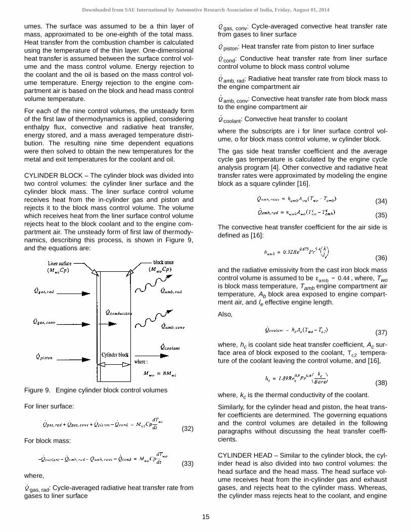
CYLINDER BLOCK – The cylinder block was divided intotwo control volumes: the cylinder liner surface and thecylinder block mass. The liner surface control volumereceives heat from the in-cylinder gas and piston andrejects it to the block mass control volume. The volumewhich receives heat from the liner surface control volumerejects heat to the block coolant and to the engine com-partment air. The unsteady form of first law of thermody-namics, describing this process, is shown in Figure 9,and the equations are:

Figure 9. Engine cylinder block control volumes

For liner surface:

(32)

For block mass:

(33)

where,

gas, rad: Cycle-averaged radiative heat transfer rate fromgases to liner surface

gas, conv: Cycle-averaged convective heat transfer ratefrom gases to liner surface

piston: Heat transfer rate from piston to liner surface

cond: Conductive heat transfer rate from liner surfacecontrol volume to block mass control volume

amb, rad: Radiative heat transfer rate from block mass tothe engine compartment air

amb, conv: Convective heat transfer rate from block massto the engine compartment air

coolant: Convective heat transfer to coolant

where the subscripts are i for liner surface control vol-ume, o for block mass control volume, w cylinder block.

The gas side heat transfer coefficient and the averagecycle gas temperature is calculated by the engine cycleanalysis program [4]. Other convective and radiative heattransfer rates were approximated by modeling the engineblock as a square cylinder [16].

(34)

(35)

The convective heat transfer coefficient for the air side isdefined as [16]:

(36)

and the radiative emissivity from the cast iron block masscontrol volume is assumed to be , where, Twois block mass temperature, Tamb engine compartment airtemperature, Ab block area exposed to engine compart-ment air, and le effective engine length.

Also,

(37)

where, hc is coolant side heat transfer coefficient, Ac sur-face area of block exposed to the coolant, tempera-ture of the coolant leaving the control volume, and [16],

(38)

where, kc is the thermal conductivity of the coolant.

Similarly, for the cylinder head and piston, the heat trans-fer coefficients are determined. The governing equationsand the control volumes are detailed in the followingparagraphs without discussing the heat transfer coeffi-cients.

CYLINDER HEAD – Similar to the cylinder block, the cyl-inder head is also divided into two control volumes: thehead surface and the head mass. The head surface vol-ume receives heat from the in-cylinder gas and exhaustgases, and rejects heat to the cylinder mass. Whereas,the cylinder mass rejects heat to the coolant, and engine

εamb 0.44=

Tc2


16

compartment air. Only the convective mode of heat trans-fer from the exhaust gas to the head surface volume wasassumed since this dominates the total exhaust port heattransfer due to high exhaust port velocities. The controlvolume analysis for the cylinder head is similar to that ofthe cylinder block.

For head surface:

(39)

For head mass:

(40)

where [4], , exhaust port heattransfer area, heat transfer coefficient, cycle aver-aged exhaust gas temperature, and cylinder headsurface temperature.

PISTON – Similar analysis was performed for the pistonsurface and the piston mass control volume. The follow-ing correlation was used to estimate the piston cooling oilheat transfer coefficient hcp [4]:

(41)

where, is Reynolds number, (2b/t)D/ , b piston cav-ity length, D piston cylindrical-cavity diameter, = D/b,

thermal conductivity of the piston cooling oil, cor-relation constant.

COOLANT IN BLOCK AND HEAD – An energy balancefor the block and head coolant results in an equationwhich describes the temperature response of the blockcoolant.

For the block:

(42)

For the head:

(43)

where, is mass flow rate of the coolant, and: coolant mass in the block and head respectively,

temperature of the coolant entering the block controlvolume, temperature of the coolant leaving the blockor entering the head volume, and temperature of thecoolant leaving head

PISTON COOLING OIL – The piston cooling oil controlvolume receives heat from the piston undercrown. Thepiston cooling flow rate as a function of engine speedwas supplied by DDC. The first law energy balance yields[22]:

(44)

SOLUTION TO THE SYSTEM OF EQUATIONS – Thedifferential equations developed in the previous sectionrepresent a coupled system of equations, which, whensolved simultaneously, represent the time dependentbehavior of the engine cylinder heat transfer model. Thesystem of equations were discretized by using the firstorder implicit scheme. The resulting matrix was solvedusing the Gaussian method with partial pivoting. Thematrix was solved iteratively due to temperature depen-dent properties and radiative heat transfer until tempera-tures converged on their new values. Convergencechecking was done by calculation of the error [16].

RAM AIR/ENGINE COMPARTMENT COOLING AIRFLOW MODEL

The coolant and the oil cooling system is designed tolimit the temperatures in the various engine parts. There-fore, how to design the cooling system for sufficient cool-ing airflow during worst case situations with maximumpower consumption has always been a major concern.The worst case situations are high ambient temperature,full load, and low vehicle speed, such as the caseencountered in going up a steep mountain in desert con-ditions.

Cooling airflow is either generated due to the ram aireffect of the vehicle motion and/or by the cooling air fan.Because of the complex geometry, complex airflow pat-terns are induced along the flow passage through thecharge-air-cooler, radiator, shroud, and over the engine.These flows are not easily understood even from goodexperimental studies. To achieve a more precise predic-tion of the engine cooling system performance, an analyt-ical model of the cooling airflow system was developedby Chang [2] in 1990.

The fan is run by a variable speed clutch drive. A pulsewidth modulator sends a pulse to the variable speedclutch. The pulse width depends on the coolant tempera-ture at the radiator top tank. For the Kysor DST faninstalled in the Freightliner truck, when the radiator toptank temperature is less than 87.8°C (190°F), the fanspeed is 0.45 times the engine speed. As the coolanttemperature increases from 87.8 to 96.1°C (190 to205°F), the pulse width changes the fan speed from 0.45to 1.12 times (a non-linear curve) the engine speed. Thefan speed factor data is based on the experimental dataand is included in the fan model in a tabular form. Duringcode validation, the program was tested for two limitingcases; one where the fan is off, and the other where thefan was run at a constant speed regardless of the vari-able clutch drive. These cases will be presented laterlabeled as fan: OFF and fan: ON respectively. All othertest runs presented are under the variable clutch drivefeature added to the software where a 3.9°C (7°F) hyster-esis is also built in the fan engagement to disengagementperiod.

The conventional cooling airflow passage consists of thegrill, condenser, charge air cooler, radiator, shroud, fan,

Q·

ex hexAep Te Thi–( )= Aephex Te

Thi

Re υoD'

ko Acp

m· c MCbMChTc1

Tc2Tc3


17

and engine compartment. One of the primary objectivesof this work was to enhance the accuracy and reliability ofthe Vehicle Engine Cooling System Simulation (VECSS)by incorporating Chang’s model [2] using performancecharacteristics of the fan, radiator, shutter, and the sys-tem installation dimensions.

The following were the outline of the specific goals:

• include the fan, radiator, and shutter performancecharacteristics,

• incorporate the branch flow in the engine compart-ment,

• incorporate the system installation physical dimen-sions, and

• identify empirical constants and necessary experi-mental data required.

FLOW RESISTANCE IN THE AIRFLOW PASSAGE –The cooling air passage is essentially treated as a one-dimensional duct network. The total core flow area of theradiator is used as the duct cross sectional area, and thecore flow hydraulic diameter is used as the diameter. Asimilar set of simplifications is applied to the other flowarea components.

The computational domain of the airflow system wasdivided into 35 equally spaced nodal points from the frontof the grill to back of the fan. The region around theengine was additionally divided in 7,10, 6 and 6 nodalpoints for the top, bottom, left and right side of the enginerespectively. Depending on the physical dimensional rela-tionship between the various components like the grill(Nodal points 1-2), CAC and condensor (Nodal points 7-13), radiator (Nodal points 16-21), and fan (Nodal points26-34), the free flow area at each nodal point was calcu-lated. The free flow area for individual components wascalculated from the component drawings supplied by therespective manufacturers. The position of the compo-nents in the system was measured in the FreightlinerFLD120 truck. The hydraulic diameter is evaluated usingthe free flow area and the wetted perimeter, which is alsocalculated from the supplied component drawings. Theengine compartment and airflow branching areas andnodal points for the Freightliner FLD 120 truck are shownin Figure 10.

Experimentally determined pressure drop data at knownairflow velocity is used to calculate the skin friction fac-tor(f) for all the components and hence the nodal points.

The free flow area, hydraulic diameter and the skin fric-tion factor at each nodal point along with fan characteris-tics and heat rejection from the radiator, condensor andCAC are used as inputs to the airflow subroutine.

The free flow area hydraulic diameter and the skin frictionfor the branching over the engine are exprimentally deter-mined by Chang [20].

Fluid head losses can be generally categorized into twosources - the skin friction and the pressure force. Theflow resistance due to skin friction is characterized by thefriction factor ‘f’. The pressure loss is [2]:

(45)

where, At total friction surface area, A cross sectionalarea, Swet wetted perimeter, and l passage length.

The secondary loss is called the minor loss, which resultsfrom the separation of the flow and secondary flow thatoccurs whenever there is a change in the cross-sectionalarea. The resistance associated with the minor losses ischaracterized by the local resistance coefficient ‘k’.

(46)

The flow resistance characteristics of the complete cool-ing circuit can be specified by the friction factor ‘f’ and thehead loss (local resistance) coefficient ‘k’ for each sectionthrough the passage. These factors are specified as adata block, and used approximately depending on thecurrent grid element in the one-dimensional passage.

The pressure losses are used to calculate the externalforce term in the governing momentum equation(described later). For the skin friction [2],

(47)

For the minor loss coefficient [2],

(48)

where, lk is the length in which minor loss occurs (m).

Both of these external force terms are added togetherwhile solving the governing equations.

It appears that it is desirable to have f-Re and k-Re [26]curves which specify these coefficients as a function ofthe Reynolds number, that is easier and directly applica-ble to the complete geometrical flow passage.

Finally, it sometimes occurs that the local resistance ishigh near the shroud, engine compartment and the joints.Abrupt contractions and expansions in these areas leadto the usage of the following empirical approximation[26]:

(49)

where, d smaller diameter (exit for contraction), D largerdiameter (inlet for contraction). As mentioned earlier, inthe calculations the effective external force term is calcu-lated after the skin friction and local resistance coeffi-cients have been evaluated.


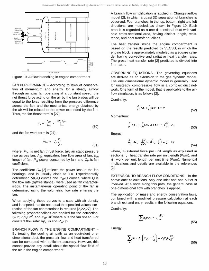
18

Figure 10. Airflow branching in engine compartment

FAN PERFORMANCE – According to laws of conserva-tion of momentum and energy, for a steady airflowthrough an axial fan operating at a constant speed, thenet thrust force acting on the air by the fan blades will beequal to the force resulting from the pressure differenceacross the fan, and the mechanical energy obtained bythe air will be related to the power expended by the fan.Thus, the fan thrust term is [27]:

(50)

and the fan work term is [27]:

(51)

where, Ffan is net fan thrust force, ∆ps air static pressurerise across fan, Afan equivalent free flow area of fan, lfanlength of fan, PW power consumed by fan, and Cfn is fancoefficient.

The coefficient Cfn [2] reflects the power loss in the fanbearings, and is usually close to 1.0. Experimentallydetermined ∆ps-Q curves and PW-Q curves, where Q isthe flow rate (∆p/resistance), were used as fan character-istics. The instantaneous operating point of the fan isdetermined using the volumetric flow rate entering thefan.

When applying these curves to a case with air densityand fan speed that do not equal the specified values, cor-rection of the fan characteristic is required [2,22,27]. Thefollowing proportionalities are applied for the correction:Q∝n, ∆ps∝n2, and PW∝n3 where n is the fan speed. Forconstant flow rate: ∆ps∝ρ and PW∝ρ.

BRANCH FLOW IN THE ENGINE COMPARTMENT –By treating the cooling air path as an equivalent one-dimensional duct, the gross air flow and heat transferredcan be computed with sufficient accuracy. However, thiscannot provide any detail about the spatial flow field ofthe air in the engine compartment.

A branch flow simplification is applied in Chang’s airflowmodel [2], in which a quasi 3D separation of branches isobserved. Four branches, in the top, bottom, right and leftdirections, are modeled, as shown in Figure 10. Eachbranch is regarded as a one-dimensional duct with vari-able cross-sectional area, having distinct length, resis-tance, and heat transfer qualities.

The heat transfer inside the engine compartment isbased on the results predicted by VECSS, in which theengine block is approximately modeled as a square cylin-der having convective and radiative heat transfer rates.The gross heat transfer rate [2] predicted is divided intofour parts.

GOVERNING EQUATIONS – The governing equationsare derived as an extension to the gas dynamic model.The one dimensional dynamic model is generally usedfor unsteady, compressible flow in a complex duct net-work. One form of the model, that is applicable to the air-flow simulation, is as follows [2]:

Continuity:

(52)

Momentum:

(53)

Energy:

(54)

where, Fl external force per unit length as explained insections. heat transfer rate per unit length (W/m), and

work per unit length per unit time (W/m). Numericalimplications and details are available in the references[2].

EXTENSION TO BRANCH FLOW CONDITIONS – In theabove duct calculations, only one inlet and one outlet isinvolved. At a node along this path, the general case ofone-dimensional flow with branches is applied.

The application of mass and energy conservation laws,combined with a modified pressure calculation at eachbranch exit and entry results in the following equations.

Continuity:

(55)

Energy:

(56)

B ranch 1

B ranch 2

B ranch 3

B ranch 4

FA N

N O D E PO IN TS

0 .70.6

0.40.30.20.1

0.5

AR

EA

(s

q.m

)

RA

DIA

TO

R

CO

ND

EN

SO

RC

HA

RG

E C

OO

LE

R

GR

ILL

A IR FLO W

A IR FLO W

SH R O U D

SH

UT

TE

R

(A rea: 0 .20)

(A rea: 0 .17)

(A rea: 0 .17)

(A rea : 0 .21)

135


19

Pressure:

(57)

(58)

The constant Ki is experimentally determined [2]. It repre-sents the pressure drop coefficient, and the pressure lossis assumed to be a function of the local Mach number.

RESULTS

The results of the VECSS model predictions will be intro-duced next under three separate categories. These are:the validation of the improved heat transfer model used inthe engine cycle analysis, the energy balance on theengine model and the implementention of the enginecompartment air flow model with and without the fanoperating.

VALIDATION OF REVISED ENGINE MODEL – The un-steady heat transfer model developed was incorporatedin the engine program developed by Mohan [4]. A similarstudy like Mohan [4] carried out had to be done in orderto validate the engine program with the enhanced heattransfer model to the steady state data on engine brakepower, brake specific fuel consumption, and exhaust tem-perature supplied by DDC at 1200 and 1800 rpm. Thiswas conducted using a stand-alone engine program withthe heat transfer model. The inputs to the model were thefuel flow rate and the engine speed given in Figures 11.The program was run until all temperatures reachedsteady state. The predicted data for A/F ratio, boost pres-sure, brake horsepower, bsfc, and exhaust temperature,show good agreement with the experimental data (within2%), Figures 12,13 ,14,15,16.

Additional predicted properties such as piston surfacetemperature, cylinder head surface temperature, andliner surface temperature variations are shown in Figures17,18,19.

The coolant temperature rise in the engine is more for1200 rpm, Figure 20, as would be expected, because oflower coolant flow rate. The predicted oil temperature outof the piston is also shown in Figure 21.

Figure 11. Fuel flow rate into the engine at two different engine speeds

Figure 12. Calculated air to fuel ratio varying with the engine load in BMEP (Bar)

Figure 13. The boost pressure with engine load


20

Figure 14. Comparison of the output power at different engine speeds

Figure 15. BSFC predictions at 1200 & 1800 rpm

Figure 16. Exhaust temperature predictions at 1200 & 1800 rpm

Figure 17. Piston surface temperature variation with load and speed

Figure 18. Cylinder head surface temperature variation with speed and load

Figure 19. Liner surface temperature with speed and load


21

Figure 20. Coolant temperature rise predictions in the engine

Figure 21. Temperature rise predictions for piston cooling oil

FIRST LAW OF THERMODYNAMICS CHECK ONENGINE HEAT BALANCE – The overall first law energybalance for the engine provides useful information on theflow of the chemical energy in the fuel. It also acts as avalidation for the VECSS software. For the control volumewhich surrounds the engine (refer to Figure 22), thesteady-state energy conservation equation is:

(59)

where, he is exhaust enthalpy, heat transfer rate to oilwhich includes friction between piston and cylinder wall,bearing friction, etc., heat transfer rate to the enginecompartment air by convection and radiation, brakepower, hf lower heating value of fuel, ha air enthalpy, mass of air, mass of fuel, and mass of coolant.

Figure 22. Control volume for energy balance on the engine

Table 2 provides the magnitude of the energy rejectionrates to the coolant and oil at various speeds and loads.As can be noted, the frictional power between the pistonand the cylinder wall as well as the bearing frictionalpower increase with increase in engine speed. The brakehorse power of the engine, the energy in the exhaustgases and the heat transfer to the coolant depend on theenergy coming into the engine, i.e., the fuel flow rate.Only about 2-3% of the energy in the fuel is unaccountedfor except at 1200 rpm where 7% is unaccounted for. Theresults are in good agreement with the published litera-ture [28].

FAN MODEL PREDICTIONS – The model was tested fortwo conditions of the fan, ON and OFF. For both thesetests the wind speed, vehicle velocity, ambient air tem-perature, atmospheric pressure, relative humidity, andradiator energy rejection were held constant.

CASE 1: Fan OFF – All the parameters given below areinputs to the airflow program, which describe the operat-ing conditions for the test.

Table 2. Magnitudes for First Law Check on Energy Balance in kW

Engine speed 1200 1350 1500 1650 1800

(rpm) kW % kW % kW % kW % kW %

Fuel in 608.8 100 670.3 100 740.5 100 715.0 100 677.8 100

Brake power 224.8 36.9 251.4 37.5 280.8 37.9 269.8 37.7 252.5 37.2

Exhaust 233.0 38.3 277.6 41.4 313.3 42.3 295.9 41.4 274.5 40.5

Coolant 78.5 12.9 89.1 13.3 96.8 13.1 95.0 13.3 93.2 13.8

Piston friction 18.7 3.07 20.7 3.09 23.8 3.21 27.7 3.87 31.3 4.62

Bearing friction 2.99 0.49 3.60 0.54 4.43 0.60 5.13 0.72 5.92 0.87

Oil splash 5.15 0.85 6.27 0.94 7.15 0.97 7.24 1.01 7.17 1.06

Piston cooling oil 1.88 0.31 2.13 0.32 2.27 0.31 2.25 0.31 2.21 0.33

Engine Compartment air 1.80 0.29 2.19 0.33 4.11 0.55 2.38 0.33 3.46 0.51

Total energy out 566.8 93.1 652.9 97.4 732.6 98.9 705.4 98.6 670.2 98.9


22

Windspeed + Vehicle velocity: 15 + 61.75 = 76.75 mphAmbient air temperature: 27°C (80.6°F)Atmospheric pressure: 101325 Pa = 1 atm.Relative humidity: 85%Radiator heat rejection: 4481.2 W

Table 3 gives the actual volume flow rate and mass flowrate predictions for the test case when fan is off. Thetable gives the number of nodes that were . The free flowarea, the friction coefficient and the predicted volumeflow rate and mass flow rate are given at the central (ormidpoint) node of each branch, i.e. node 18 for mainbranch, node 4 for branch 1, node 5 for branch 2, andnode 3 for branch 3 and 4.

Figure 23. Velocity and airflow rate when fan is OFF*Note: Grill (1-2), Condenser and CAC (7-13), Radiator(16-21), Shroud (24-32), Fan(26-34)

Figure 24. Temperature and density variation when fan is OFF

*Note: Grill (1-2), Condenser and CAC (7-13), Radiator(16-21), Shroud (24-32), Fan(26-34)

Figure 25. Pressure variation when fan is OFF for main branch


Figure 23 and Figure 24 depicts the airflow velocity andthe actual volume flow rate at each node in the mainbranch and the temperature and density variation plotsrespectively. As the air flows over the radiator, energytransfer from the radiator increases the temperature ofthe air, decreasing the density (node points 14 to 21).This results in increase in the actual volumetric flow rate,since the mass flow is conserved. For the case I, the airpressure keeps decreasing from the front of the grill untilthe end of the fan as shown in Figure .

CASE 2: Fan ON – The input parameters which describethe operating condition for this test are as follows,

Wind speed + Vehicle velocity: 15 + 61.75 = 76.75 mphAmbient air temperature: 27°C (80.6°F)Atmospheric pressure: 101325 Pa = 1 atm.Relative humidity: 85%Radiator heat rejection: 4481.2 W

Table 4 gives the predicted volume flow rate and massflow rate for the central nodes for each branch. Figure 26shows the rise in temperature of the air as it passes overthe radiator and the corresponding drop in pressure. Thisincreases the actual volumetric flow rate in the radiator asshown in Figure 27. The pressure of the air decreasesuntil nodal point 25, and then rises from 26 to 35 becauseof the condition that the fan is ON as shown in Figure 27.

Table 3. Predictions of AIRFLOW model when the fan is OFF

Branch At node

Free flow area

(sq.m)

Friction Coefficient

Temperature(deg C)

Actual volume

flow rate (ACMS)

Mass flow rate (kg/s)

Main 18 0.51 0.21 41.56 2.91 3.27

1 4 0.21 1.20 82.39 0.74 0.72

2 5 0.20 3.80 81.22 0.08 0.09

3 3 0.17 3.90 81.72 1.11 1.23

4 3 0.17 3.40 81.83 1.17 1.24

Table 4. Predictions of AIRFLOW model when the fan is ON

Branch At node

Free flow area

(sq.m)

Friction Coefficient

Temperature(°°°°C)

Actual volume

flow rate (ACMS)

Mass flow rate (kg/s)

Main 18 0.51 0.21 52.00 4.01 4.48

1 4 0.21 1.20 70.72 1.86 1.86

2 5 0.20 3.80 69.72 0.46 0.54

3 3 0.17 3.90 70.17 0.96 1.07

4 3 0.17 3.40 70.11 0.99 1.01


23

Figure 26. Temperature and density variation when fan is ON


Figure 27. Velocity and airflow rate when fan is ON*Note: Grill (1-2), Condenser and CAC (7-13), Radiator(16-21), Shroud (24-32), Fan(26-34)

Figure 28. Pressure variation when fan is ON for main branmch


All the figures show the variation of the indicated parame-ter in the MAIN branch at each node. Comparisonbetween Figure 23 and Figure 27 shows that for the con-dition that the fan is ON, the airflow velocity and volumeflow rate at all node points in the main branch is muchhigher than when the fan is OFF. Since, the inlet tempera-ture condition, and the radiator energy rejection is thesame for both cases, the temperature variation and thedensity variation along the nodes remains the same. Forfan ON condition, the pressure variation curve (Figure27), shows a drop in the pressure from nodes 1 to 26 dueto the system resistance and then shows a steep rise inpressure from nodes 26 to 35 due to fan work. Asopposed to this, the fan OFF condition shows a continu-ous drop in pressure from nodes 1 to 35 (Figure 25).

CONCLUSIONS

The main objective of this paper was to develop theVECSS (ver 8.1) software program with the addition ofcooling airflow model and to validate the calculatedengine parameters as compared to the experimental datafor the improved heat transfer model. The software pro-gram had to be enhanced and upgraded to the truck con-figuration for which the steady-state and transient truckdata were recorded. These data are compared to theVECSS model output data in the accompanying paper,part 2 by Arici, et al [5]. The one-dimensional, transient,compressible ram air / engine compartment airflow modeldeveloped by Chang [2] was incorporated in the VECSSprogram. This work enhanced the capability of theVECSS program to accurately predict the airflow over theradiator and in the engine compartment. The additionalfeature gives the user the capability to study the tempera-ture and pressure variation in the cooling airflow systemwith a change in the system installation characteristics.The one-dimensional, unsteady engine heat transfermodel was developed and incorporated into Mohan’s [4]engine cycle analysis model so that time varying piston,head, and liner temperatures could be evaluated.

In the process of validating the program the followinghave been achieved:

1. The engine cycle analysis model that incorporatedthe heat transfer model predicted engine brakepower, brake specific fuel consumption, and exhaustgas temperature in good agreement with DDC’ssteady state experimental data at engine speeds of1200 and 1800 rpm for which it was validated (within1.5%).

2. The radiator model developed was validated withBehr McCord’s steady state heat rejection data sothat the agreement was within 2%.

3. The oil cooler model was modified, and extensivelyvalidated against DDC’s effectiveness data (within2%), and incorporated into the VECSS.


24

4. The first law energy balance check on the enginecycle analysis model showed good agreement withthe energy in the fuel.

ACKNOWLEDGEMENTS

The authors acknowledge the continued financial andtechnical support by Kysor Cooling Systems of theSchwitzer Group. In particular, we want to express ourappreciation to Vince Ursini from Kysor for his efforts incollecting the vehicle test data used for the validation,and valuable comments on the thermostat and fan mod-els. Detroit Diesel Corporation is gratefully acknowledgedfor providing us with extensive test data on their Series60 12.7 L engine and also other engine related informa-tion including help in modeling the oil circuit. John Fisher,Chris Prichard, and Dr. Dan Ducu of DDC gave us signifi-cant help and feedback on our modeling and validationeffort.

REFERENCES

1. Ursini, V.J., “A Computer Simulation Program for Evaluationof the Cooling System Performance of a Diesel PoweredTruck”, Master’s Thesis, Michigan Technological University,1982.

2. Chang, X., “Prediction and Analysis of Truck Engine Cool-ing Airflow by means of a One-dimensional Transient Com-pressible Flow Model”, Ph.D. Thesis, MichiganTechnological University, 1990.

3. Ursini, V.J., “Ram Air as a Function of Wind Speed”, KysorEngineering Test Report 85010, April 11, 1987.

4. Mohan, K.V., “A Computer Simulation of the TurbochargedDI Diesel Engine as an Enhancement of the Vehicle EngineCooling System Simulation”, Master’s Thesis, MichiganTechnological University, 1997.

5. Arici, O., Johnson, J.H., Kulkarni, A., “The Vehicle EngineCooling System Simulation. Part 2 - Model Validation UsingTransient Data”, SAE Paper 1999 - 01 - 0241, 1999.

6. Chiang, E.C., Ursini, V.J., and Johnson, J.H., “Developmentand Evaluation of a Diesel Powered Truck Cooling SystemComputer Simulation Program,” SAE Paper 821048, 1982.

7. Ursini, V.J., Chiang, E.C., and Johnson, J.H., “A ComputerCooling System Study of a Diesel Powered Truck for Con-trol of Transient Coolant, Oil, and Cab Temperatures”, SAEPaper 821049, 1982.

8. Savonen, C.L., “Modeling of Thermal Characteristics of Oiland Coolant Flows within a Diesel Engine Cooling Systemand a Parametric Study of Variables Influencing its Perfor-mance”, Master’s Thesis, Michigan Technological Univer-sity, 1984.

9. Savonen, C.L., Chiang, E.C., and Johnson, J.H., “TheEffects of Ambient Temperature and Vehicle Load on a Die-sel Powered Truck Cooling System Performance Using aComputer Simulation Program”, SAE Paper 841710, 1984.

10. Chellaiah, S., “The Development and Validation of a Com-puter Code for the Simulation of Advanced Low Flow Die-sel Truck Cooling Systems”, Master’s Thesis, MichiganTechnological University, 1984.

11. Chiang, E.C., Chellaiah, S., Johnson J.H., “Modeling ofConvective Heat Flow in Radiators for Coolant TemperaturePrediction”, ASME Paper 85-WA/HT-22, 1985.

12. Xu, Z., Johnson, J.H., and Chiang, E.C., “A SimulationStudy of a Computer Controlled Cooling System for a Die-sel Powered Truck”, SAE Paper 841711, 1984.

13. Xu, Z., Johnson, J.H., “The Design and Testing of a Com-puter-Controlled Cooling System for a Diesel-PoweredTruck”, SAE Paper 841712, 1984.

14. Keller, J.R., “The Validation of a Low-Flow Diesel TruckCooling System Model and a Parametric Study of AmbientTemperatures, Temperature Control Components and Set-tings”, Master’s Thesis, Michigan Technological University,1984.

15. Keller, J.R. Chiang, E.C., Johnson, J.H., “The ThermostatCharacteristics and Its Effects on Low-Flow Engine CoolingSystem Performance”, SAE Paper 900904, 1990.

16. Chapman, K.S., “The Enhancement and Validation of aVehicle Engine Cooling System Simulation for Use as aCooling System Design Tool”, Master’s Thesis, MichiganTechnological University, 1987.

17. Chapman, K.S., Johnson, J.H., and Chiang, E.C., “TheEnhancement and Validation of a Vehicle Engine CoolingSystem Simulation for a Heavy Duty Diesel Truck”, SAEPaper 880601, 1988.

18. Hovin, L.E., “A Computer Simulation of a MicroprocessorControlled Cooling System for a Heavy Duty Diesel Truck”,Master’s Thesis, Michigan Technological University, 1987.

19. Hovin, L.E., Chiang, E.C., Johnson, J.H., “Design & Com-puter Simulation of Microprocessor Controlled LubricatingOil Cooling System for Truck Diesel Engines”, SAE Paper880488, SAE Trans., Vol. 97, 1988.

20. Chang, X., Chiang, E.C., Johnson, J.H., “A One-Dimen-sional Transient Compressible Flow Model for Cooling AirFlow Rate Computation”, SAE Paper 900721, 1990.

21. Mohan, K.V., Arici, O., Yang, S.L., Johnson, J.H., “A Com-puter Simulation of the Turbocharged Diesel Engine as anEnhancement of the Vehicle Engine Cooling System Simu-lation”, SAE Paper 971804, 1997.

22. Kulkarni, A.J., “The Vehicle Engine Cooling System Simu-lation With the Addition of a Compressible Cooling AirflowModel - Validation Using Transient Experimental Data”,Master’s Thesis, Michigan Technological University, 1998.

23. Ocvirk, F.W., and Dubois, G.C., “Analytical Derivation andExperimental Evaluation of Short Bearing Approximationfor Full Journal Bearing”, Report 1157, N.A.C.A., 1953.

24. French, C.C.J., “Piston Cooling”, SAE Paper 720024, 1972.

25. Huang, C.C.D., “A Dynamic Computer Simulation Model fora Automobile Passenger Car Compartment Control andEvaluation”, Ph.D. Thesis, Michigan Technological Univer-sity, 1998.

26. White, F.M., Fluid Mechanics, McGraw-Hill Book Co., 1979.

27. Jorgensen, R., Fan Engineering, McGraw-Hill Book Co.,1965.

28. Heywood, J.B., Internal Combustion Engine Fundamentals,McGraw-Hill Book Company, 1988.

29. Detroit Diesel Corporation, Memo, March 1998.


the vehicle engine cooling system simulation

Documents