NBER WORKING PAPER SERIES

THE U.S. DEBT RESTRUCTURING OF 1933:CONSEQUENCES AND LESSONS

Sebastian EdwardsFrancis A. LongstaffAlvaro Garcia Marin

Working Paper 21694http://www.nber.org/papers/w21694

NATIONAL BUREAU OF ECONOMIC RESEARCH1050 Massachusetts Avenue

Cambridge, MA 02138November 2015

Sebastian Edwards is with the UCLA Anderson School and the NBER. Francis A. Longstaff is withthe UCLA Anderson School and the NBER. Alvaro Garcia Marin is with the Universidad de Chile.We are grateful for the capable research assistance of Colton Herbruck, Scott Longstaff, and Yuji Sakurai.All errors are our responsibility. The views expressed herein are those of the authors and do not necessarilyreflect the views of the National Bureau of Economic Research.

NBER working papers are circulated for discussion and comment purposes. They have not been peer-reviewed or been subject to the review by the NBER Board of Directors that accompanies officialNBER publications.

© 2015 by Sebastian Edwards, Francis A. Longstaff, and Alvaro Garcia Marin. All rights reserved.Short sections of text, not to exceed two paragraphs, may be quoted without explicit permission providedthat full credit, including © notice, is given to the source.

The U.S. Debt Restructuring of 1933: Consequences and LessonsSebastian Edwards, Francis A. Longstaff, and Alvaro Garcia MarinNBER Working Paper No. 21694November 2015JEL No. E43,E44,E65

ABSTRACT

In 1933, the U.S. unilaterally restructured its debt by declaring that it would no longer honor the goldclause in Treasury securities. We study the effects of the abrogation of the gold clause on sovereigndebt markets, the Treasury's ability to issue new debt, investors' willingness to hold Treasury bonds,and on the Treasury's borrowing costs. We find that the restructuring was followed by a flight to qualityin the sovereign market. Despite this, there was little effect on the Treasury's ability to sell new debtor the willingness of investors to roll over restructured debt. The Treasury incurred a marginally highercost of capital by issuing new bonds without the gold clause.

Sebastian EdwardsUCLA Anderson Graduate School of Management110 Westwood Plaza, Suite C508Box 951481Los Angeles, CA 90095-1481and NBERsebastian.edwards@anderson.ucla.edu

Francis A. LongstaffUCLAAnderson Graduate School of Management110 Westwood Plaza, Box 951481Los Angeles, CA 90095-1481and NBERfrancis.longstaff@anderson.ucla.edu

Alvaro Garcia MarinUniversidad de Chile Department of Economics Diagonal Paraguay 257 Santiago, Chile algarcia@fen.uchile.cl

1. Introduction

A recurrent myth regarding the U.S. economy is that the federal government hasnever defaulted on its debt. This notion comes up every time the debt ceiling isreached and Congress wrangles about increasing the public debt limit. Considerthe following quote from White House Press Secretary James “Jay” Carney in2011:1

“The United States government has never defaulted on its obligationsto pay its debt. It has never, ever missed a payment. This is one of thereasons that “flights to quality” typically involve buying U.S. Treasurydebt. Uniquely in the history of sovereign borrowers, the United Stateshas paid when it said it would pay.”

However, the U.S. did restructure its debt unilaterally during the first ad-ministration of Franklin D. Roosevelt, and imposed a 41 percent loss on investors.On June 5, 1933, Congress passed a joint resolution altering the nature of debtcontracts retroactively. Gold clauses, which established that debts were to bepaid in “gold coin,” were eliminated for all debts (public and private). This wasthe first step in what would become one of the largest transfers of wealth (fromcreditors to debtors) in the history of the world. The next step took place onJanuary 31, 1934, when the U.S. dollar was officially devalued by 41 percent—theprice of gold went from $20.67 to $35.00 per ounce.2 In February 1935, the cyclewas closed when the Supreme Court, in a 5 to 4 decision, ruled that the abro-gation of the gold clauses was constitutional. Investors collected their monies indepreciated dollars. The debts involved (both public and private) amounted toalmost 1.7 times the nation’s GDP. Although in recent years most of the popularpress and news analysts have ignored this episode, a number of scholars haveacknowledged it. For example, Reinhart and Rogoff (2009, p. 113) include it intheir list of sovereign defaults.3

An important question, and one that has not been addressed in detail in

1Carney (2011) in http://www/cnbc.com/id/43140915. The distinction betweenfederal and state debt is important. A number of states defaulted during the 19thand 20th centuries. For example, see MacDonald (2013) and Ang and Longstaff(2013).2This number is close to the historical average market haircut of 37–40 percentcomputed independently by Benjamin and Wright (2008), Cruces and Trebesch(2013), and Edwards (2015a).3See also Friedman and Schwartz (1963), Kroszner (1999), and Edwards (2015b).

1

the literature, is the following: What were the consequences of the Treasuryreneging on its promises and implementing a generalized breach on contracts?Understanding this issue is not only important from a historical perspective, itis also relevant to understanding current events and to shed light on the likelyconsequences of modern defaults, including the debt restructurings in Greece andArgentina. According to traditional economic theory, the violation of contractsshould have a number of negative consequences for debtors. Among other things,after defaulting and imposing losses on investors, debtors should have troubleaccessing capital markets and issuing new debt, the cost of capital should increasesignificantly, liquidity should be hampered, and there should be a “‘stigma effect”on new debt. At the aggregate level, a major credit event and a generalizedbreach of contracts should result in increased uncertainty and a reduction ininvestment and, thus, in a lower growth rate. This was indeed the view takenby Friedman and Schwartz (1963, p. 699), who in the concluding chapter oftheir monumental A Monetary History of the United States: 1857–1960, arguethat although the devaluation of the U.S. dollar had a positive effect on liquidity,“the abrogation of the gold clauses . . . had the opposite [negative] effect bydiscouraging business investment.” However, they offer no empirical evidence onthe actual consequences of this chapter of U.S. history on investment or othervariables related to the functioning of the capital markets.

Interestingly, since the publication of Friedman and Schwartz (1963), therehave been few analyses of the consequences of the abrogation of the gold clauseand the unilateral restructuring of the U.S. debt. Meltzer (2003) provides adiscussion of the abrogation proper, and of how yields on gold-linked prices im-pacted the discussions at the Federal Reserve, but provides no analysis of howthis event affected real or financial variables. The same may be said about othermajor works that cover this period, including research by Temin (1991), Eichen-green (1992), Romer (1992), and Bernanke (2000). Important exceptions includeMcCulloch (1980) who analyzed the consequences of banning indexed bonds be-tween 1933 and 1977, and Kroszner (1999) who studied the evolution of differentsecurities’ prices over a two-day window surrounding the Supreme Court’s rulingon the gold clause cases in February 1935.

The purpose of this paper is to fill this void in the literature and to analyzein depth the consequences of the abrogation of the gold clause. By studying indetail this important and massive episode we hope to add to the understandingof what happens in the aftermath of a major unilateral restructuring. Four keyresults emerge from this analysis.

First, we find that after the abrogation of the gold clause, yields on thedollar denominated debt of the remaining high credit quality sovereigns suchas the United Kingdom, France, and Switzerland quickly declined to near-zero

2

or even slightly negative values. This phenomenon closely resembles the classicflight to quality pattern in the wake of major credit events such as the LongTerm Capital Management (LTCM) crisis following the Russian default in 1998,or the recent global financial crisis following the default of Lehman Brothers.

Second, we find that despite the apparent global flight to quality, the Trea-sury experienced little or no difficulty in issuing new debt. In particular, aftercontrolling for key debt features, we find that Treasury auctions were just asoversubscribed after the abrogation as before.

Third, we find that Treasury debtholders whose bonds were involuntarilyrestructured were only slightly less willing to roll over these bonds into newTreasury securities at maturity as before the abrogation. Thus, there is littleevidence that holders of restructured Treasury debt “voted with their feet” bystigmatizing new debt issues.

Fourth, we examine whether the abrogation of the gold clause affected theTreasury’s cost of debt by contrasting the yields on bonds with a gold clause tothe yields on newly issued bonds without the gold clause. We find that prior tothe devaluation, there was no significant difference in the yields of the two typesof bonds. After the devaluation, however, gold clause bonds traded at a fourto eight basis point premium to non-gold clause bonds. Curiously, the premiumfor gold clause bonds persisted even after the Supreme Court decision. Onepossible interpretation of this result is that investors continued to believe thata return to the gold standard might occur once macroeconomic fundamentalsimproved. Another possible interpretation is that the market believed there wassome probability that the Supreme Court would reverse itself and grant somecompensation to holders of gold clause securities. Indeed, during the years tocome, a number of lawsuits regarding the abrogation made it through the courtsystem. The Supreme Court, however, refused to hear any of these cases.

By studying the effects of the U.S. abrogation of the gold clause, this papercontributes to the general literature on sovereign debt restructurings and defaults.Important papers in that literature include Eaton and Gersovitz (1981), Mendozaand Yue (2012), Reinhart and Rogoff (2004, 2011), Lindert and Morton (1989),and Cruces and Trebesch (2013). Our analysis differs from previous work inseveral respects. First, we focus on an episode in an advanced country which wasone of the two financial centers of the world at the time the debt was unilaterallyrestructured. Most previous work on this subject has focused on the effects ofsovereign restructurings on economic conditions in periphery countries. Second,we use daily time series on bond returns over a span of three years to analyze thebehavior of key variables around key moments in this episode. In contrast, in hisimportant contribution, Kroszner (1999) concentrates on returns during two dayssurrounding the Supreme Court’s decision on the gold clause cases (February 16–

3

18, 1935). Third, we use daily data to analyze whether the Treasury had problemsrolling over its maturing debt. This issue has been addressed recently by Crucesand Trebesch who studied how soon emerging countries that restructured theirdebts between 1978 and 2010 could assess capital markets again. Fourth, we useour data set to analyze the extent to which the unilateral change in contractsincreased the cost of public debt in the U.S. Fifth, we complement the workof Bernanke (2000) and others by comparing daily yields on sovereign debt inthe U.S. and other advanced nations under different circumstances, (the UnitedKingdom, France, and Switzerland).

The rest of the paper is organized as follows. Section 2 provides historicalperspective on the abrogation of the gold clause in 1933, the subsequent officialdevaluation of the dollar in 1934, and the Supreme Courts gold clause decisionsin 1935. Section 3 examines whether a flight to quality occurred in the sovereigndebt markets. Section 4 studies the effects on the Treasury’s ability to issue newdebt. Section 5 examines whether there was any stigma attached to new debtissued by existing bondholders. Section 6 studies the effects on the Treasury’sborrowing costs. Section 7 summarizes the results and discusses their implica-tions.

2. Historical Background

On April 5, 1933, President Franklin D. Roosevelt, who had been in office forexactly one month, issued an executive order requiring people and businesses tosell, within three weeks, all their gold holdings to the government at the officialprice of $20.67 per ounce. The Secretary of the Treasury Will Woodin tried toexplain the policy by saying that “gold in private hoards serves no useful purposeunder current circumstances. When added to the stock of the Federal ReserveBanks it serves as a basis for currency and credit. This further strengthening ofthe banking structure adds to its power of service toward recovery.”4

The weeks that followed changed America. Between March and June 1933,Congress passed legislation that would fundamentally alter the way the economyfunctioned, and would set the basis for the welfare state. On March 5, 1933,President Roosevelt convened Congress into an extraordinary session, and thelegendary “Hundred Days” began.5

4The New York Times, “President Invokes Law on Hoarders,” April 6, 1933.5For a contemporary description of that period see, for example, Moley (1939).

4

2.1 Abrogation and Devaluation

While the foundations of the American economy were being changed by one act ofCongress after another, the gold saga initiated with the April 5, 1933, executiveorder continued to unfold. On April 16, The New York Times reported thatglobal financial markets “were in confusion as a result of the uncertainty thatstill surrounds the United States Treasury Department’s attitude with respectto gold exports.” The previous day, a Treasury spokesman had stated that onlythree licenses for gold exports had been granted since April 6, and that newrequests would be judged “on their merits.” The Times commented that thiswas “more or less meaningless in the circumstances.”6

On April 19, 1933, President Roosevelt clarified things, and explained thatthe country was, in effect, “off gold.” He told the press corps:

“If I were to write a story, I would write it along the lines of a decisionthat was actually taken last Saturday, but which really goes into effecttoday, by which the government will not allow the exportation of gold,except earmarked gold for foreign governments, of course, and balancesin commercial exchange.”

He then explained that the main goal of abandoning the monetary system thathad prevailed since 1879 was to help the agricultural sector, which had beenstruggling for over a decade. The price of gold had been fixed at $20.67 perounce since 1834. He said: “The whole problem before us is to raise commodityprices.” The official announcement came the next day through Executive OrderNo. 6111, which stated that “until further . . . order the export of gold coin, goldbullion or gold certificates from the United States . . . are hereby prohibited . . . ”

The reaction of global currency markets was instantaneous. In one day thedollar, which had been stable until that point in its historical levels, lost 9.8percent of its value relative to the Pound Sterling, and 7.8 percent relative tothe French Franc, one of the few currencies that was still on the gold standard.Astute observers noticed that in spite of the major changes that had taken placein the course of two weeks, there was a fundamental contradiction; while it wasillegal for Americans to hold the metal, and it was prohibited to make goldpayments to foreigners, the official price was still $20.67 per ounce. On the otherhand, the value of the currency in global financial centers fluctuated accordingto market forces. It would take the government almost a year to deal with thisthorny issue and to eliminate the inconsistency of a dual exchange rate regime

6“Foreign Currencies Continue to Advance against the Dollar,” The New YorkTimes, April 16, 1933. p. N7.

5

where market and official exchange rates could differ by significant margins.

The next step came on May 12, 1933, when Congress passed the Agricul-tural Adjustment Act (AAA). Title III of this legislation included the “ThomasAmendment”— named after its author, Oklahoma’s Senator Elmer Thomas—which authorized the President to increase the official price of gold to up to $41.34an ounce. Less than a month later, on June 5, a joint resolution of Congress an-nulled all existing contracts denominated in gold dollars and stated that no suchcontracts could be written in the future. This came to be known as “the abro-gation of the gold clauses.” The government claimed that the Joint Resolutionof June 1933 didn’t imply “a repudiation of contracts.” Since gold paymentshad been suspended in April, all Congress had done was clarify that “the holderof an obligation cannot specify in what type of currency [gold or paper money]the contract is payable.” The Secretary of the Treasury was quick to state thatthe annulment of the gold clause “from all contracts and obligations, public andprivate, should have no depreciating effect on their value.”7

The amount of debt affected by the abrogation of the gold clause was enor-mous, almost twice as large as the nation’s gross domestic product. Since WorldWar I most public debt—bonds, notes and certificates—were payable in “goldcoin” and many private bonds issued by railway companies and public utilities, aswell as commercial and residential mortgages, included gold clauses.8 Accordingto the administration’s estimates in 1933, $120 billion dollars of debt—nationalincome was only slightly higher than $66 billion—were linked to the value of gold;of this, $100 billion corresponded to private debt and $20 billion to governmentdebt.

In early August 1933, administration lawyers began to explore the possibilityof the government buying—on consignment—newly minted gold at a price thatexceeded the official parity. Original discussions revolved around a price of $28per ounce.9 On August 29, the plan was announced through Executive OrderNo. 6261. This plan, which was the brainchild of Professor George F. Warren ofCornell University, moved the U.S. closer to an official devaluation of the dollar interms of gold. As explained by President Roosevelt himself, the price to be paidfor newly minted gold was to be “equal to the best price obtainable in the freegold markets of the world.”10 On October 22, the President announced during

7Roosevelt signs gold clause ban,” The New York Times, April 6, 1933. p. 35.8According to the Liberty Loan Legislation of 1917–1919, the U.S. was not al-lowed to issue long-term debt that was not indexed to gold. Thus, all long termfederal public debt included a gold clause (see U.S. Treasury Department (1921)).9Acheson (1965), pp. 177-178.10Roosevelt (1938, Vol. 1, p. 352). For a detailed discussion of this period, see

6

his Fourth Fireside Chat, that he was expanding the gold buying program. Hesaid that the “United States must take firmly in its own hands the control ofthe gold value of our dollars.”11 During the months that followed, prices paidfor gold increased steadily from $29.01 per ounce on October 21, to $31.96 onOctober 30, $33.32 on November 11, and $34.06 on December 30. It stayed atthat level until January 31, 1934.

On January 31, 1934, President Roosevelt officially devalued the dollar byfixing the new price of gold at $35 an ounce. Conservatives deplored the decision,and argued that it would inevitably lead to a steep decline in America’s power.Others, including the farm lobby, were disappointed by what they consideredan insufficient adjustment in the value of the dollar. In explaining the decision,President Roosevelt said that the devaluation was necessary, since the nation hadbeen “adversely affected by virtue of the depreciation in the value of currenciesto other governments in relation to the present standard of value.”12

In Figure 1 we present weekly data on the USD/Sterling and USD/FrenchFranc spot exchange rates between 1921 and 1936. Both rates are in the form ofdollars per unit of foreign currency. This figure captures: (a) the return of theU.K. to gold in May 1925; (b) the abandonment of gold by the U.K. in September1931; (c) the re-pegging of the Franc to gold in late 1926; (d) the abandonmentof the gold standard by the U.S. in April 1933; (e) the period of a “managed”currency between April 1933 and January 1934; and (f) the adoption of the newdollar gold parity at $35 per ounce in January 1934.

2.2 The Supreme Court Rulings

Investors that had purchased securities protected by the gold clause—that issecurities that specifically stated that payment was to be made “in gold of thepresent weight and fineness”—claimed that the Joint Declaration of June 1933was unconstitutional. Various lawsuits were filed and made their way throughthe court system. Four of them got to the Supreme Court, and were heard onJanuary 8–11, 1935.

The first two cases had to do with private debts. One referred to a railroadbond (Norman v. Baltimore & Ohio Railroad Co.), and the second to a mortgagedebt secured by a bond denominated in gold dollars (United States v. Bankers

Edwards (2015b) and the references cited therein.11Roosevelt (1938, Vol. 1, p. 426).12Presidential Proclamation No. 2072. See Roosevelt (1938, Vol. 3, pp. 67-76).

7

Trust). The third case involved a government bond in the series of the FourthLiberty Loan issued on October 15, 1918. The covenants for this 4.50 percentgold bond expressly stipulated that “the principal and interest hereof are payablein United States gold coin of the present standard of value” (Perry v. UnitedStates). As in the Norman and Bankers Trust cases, the holder of this bondasked to be paid $35 per troy ounce of gold. The Treasury refused, and made apayment in paper dollars using the old parity of $20.67.per ounce of gold. Thefourth case referred to a gold certificate (Nortz v. United States).

In these four cases the question before the Court was whether Congresshad the constitutional power to alter contracts. Under the Constitution, couldCongress annul private and public debt promises and, in the process, affect thewealth of debtors and creditors? And, if in the opinion of the Court, Congresshad exceeded its power, what were the damages?

The Supreme Court ruled on February 17, 1935. In all cases the vote was5 to 4 in favor of the government position. However, the majority used differentarguments to decide each of the cases. In the private debt cases the majority,led by the Chief Justice Charles Evans Hughes, pointed out that according tothe Constitution, Congress had the power to conduct monetary policy; morespecifically, under Article 1, Section 8, Congress had the power to “coin money,[and] regulate the value thereof.” Thus, based on this constitutional prerogativeCongress could invalidate private contracts if they interfered with such power.

In the case involving the Liberty Bonds, the majority used a different rea-soning. According to the opinion, which was also written by the Chief Justice,Congress could not abrogate the gold clause for government debt. The reasonwas that although Congress was allowed by the Constitution to regulate thevalue of money, it could not use that power to invalidate obligations arising fromanother of its constitutional powers, the power to borrow money on the creditof the United States. Thus, concluded the majority, the abrogation of the goldclause for government debt was unconstitutional. However, the Court added,since gold holdings by private parties had been forbidden since May 1933, if theclaimant received payment in bullion for his Liberty Bond, he would be obligedto sell it immediately to the Treasury at $20.67 an ounce. Thus, even though theabrogation of the gold clause for government debt was unconstitutional, therewere no damages.

There was a single dissent signed by the four conservative members of theCourt, known as the “Four Horsemen.” It was delivered by Justice James C.McReynolds, who said: “The Constitution as many of us understood it, theinstrument that has meant so much to us, is gone.” He then talked about thesanctity of contracts, government obligations, and repudiation under the guise oflaw. It was clear, he stated, that Congress had the power “to adopt a monetary

8

system. But because Congress may adopt a system, it doesn’t follow that thismay be enforced in violation of existing contracts.” He ended his allocution withstrong words: “Shame and humiliation are upon us now. Moral and financialchaos may be confidently be expected.”13

3. Was There a Flight to Quality?

As discussed by Oliner and Rudebusch (1992), Gertler and Gilchrist (1993), Langand Nakamura (1995), Bernanke, Gertler, and Gilchrist (1996), Eichengreen,Hale, and Mody (2001), Longstaff (2004), Caballero and Krishnamurthy (2008),Pavlova and Rigobon (2008), Beber, Brandt, and Kavajecz (2009), Guerrieriand Shimer (2014), and others, major economic and financial shocks are oftenassociated with a flight to quality. In a classic flight to quality, the prices of theassets considered to be the safest in the market are rapidly bid up as investorsrebalance their portfolios towards less risky assets, resulting in a sharp increasein the spread between these and other lower quality assets. Recent examples offlights to quality include the Russian default in August 1998 which triggered theLTCM crisis, the aftermath of the Lehman default in 2008 in which a global flightto quality led to short-term Treasury yields approaching zero, and the Greek debtcrisis which resulted in German sovereign yields reaching zero or negative valuesin response to the flight of investors from the threat of broader credit contagion.

In this section, we study whether the abrogation of the gold clause by theU.S. resulted in a similar type of flight in the global financial markets. Prior tothe abrogation, the U.S. with its Aaa rating was viewed as one of the largest andhighest quality sovereign borrowers in the world, particularly given the numeroussovereign defaults which had occurred during the 1930–1932 period.14 After theabrogation, however, disillusioned investors may have turned to the highest-ratedbonds issued by the strongest remaining sovereign borrowers.

In examining this issue, we make use of the fact that many sovereigns hadissued dollar denominated bonds that were listed on the New York Stock Ex-change during the 1930s. Thus, we can contrast the yields on these sovereignbonds directly with those for comparable Treasury bonds since the currency isheld fixed. Among the bonds with the highest Moody’s Investor Services (1933)

13James C. Mc Reynolds “Corrected Dissent in the Gold Clause Cases,” Ten-nessee Law Review, Vol. 18, 1945.14A partial list includes Australia, Austria, Belgium, Brazil, Chile, Colombia,Germany, Greece, Hungary, Italy, Mexico, Peru, Poland, Romania, Spain, andTurkey. See Reinhardt and Rogoff (2009).

9

ratings was the Aaa-rated United Kingdom 5.50 percent bond maturing Febru-ary 1937, the Aa-rated French 7.50 percent bond maturing April 1941, and theAa-rated Swiss 5.50 percent bond maturing April 1946. Interestingly, the non-dollar denominated debt of these three countries received only a rating of A fromMoody’s.15 This suggests that these three sovereigns viewed the timely paymentof coupons and principal on their dollar denominated New York Stock Exchangelisted bonds as their highest priority. Thus, these bonds may well have beenviewed as among the safest bonds available in the markets.

These three countries provide an interesting sample of very diverse coun-tries. The U.K. had abandoned the gold standard in September 1931, and hadallowed the value of Sterling to fluctuate in response to market forces. It had,however, established the “Exchange Equalization Account” in 1932, a fund usedto intervene in the market from time to time in order to avoid very large fluc-tuations in the exchanges. France, on the other hand, continued to be firmly“on gold.” It had returned to the gold standard in 1928 at a highly undervaluedcurrency value, and had been accumulating bullion at a very fast rate during theearly 1930s. Switzerland was also on gold, and it was universally considered tohave a strong fiscal and financial position. The above points confirm that afterthe abrogation of the gold clause in the U.S., France and Switzerland would havebeen considered strong countries, safe havens with quality debt. The fact thatthe U.K. had already made adjustments and had given up attempts to cling tothe pre-War parity was also a positive, since it had put an end to uncertainty.

We collected daily closing price quotations for the U.K., French, and Swissbonds described above. These three bonds are matched to the 2.75 percentTreasury notes maturing December 1936, the 3.375 percent Treasury bonds ma-turing 1941–1943, and the 3.750 percent Treasury bonds maturing 1946–1956,respectively. The close match in the maturities of the sovereign and Treasurybonds ensures that their yields are directly comparable.16 The price quotationsfor all the bonds are hand collected from the Bond Sales of the New York StockExchange section of The New York Times.

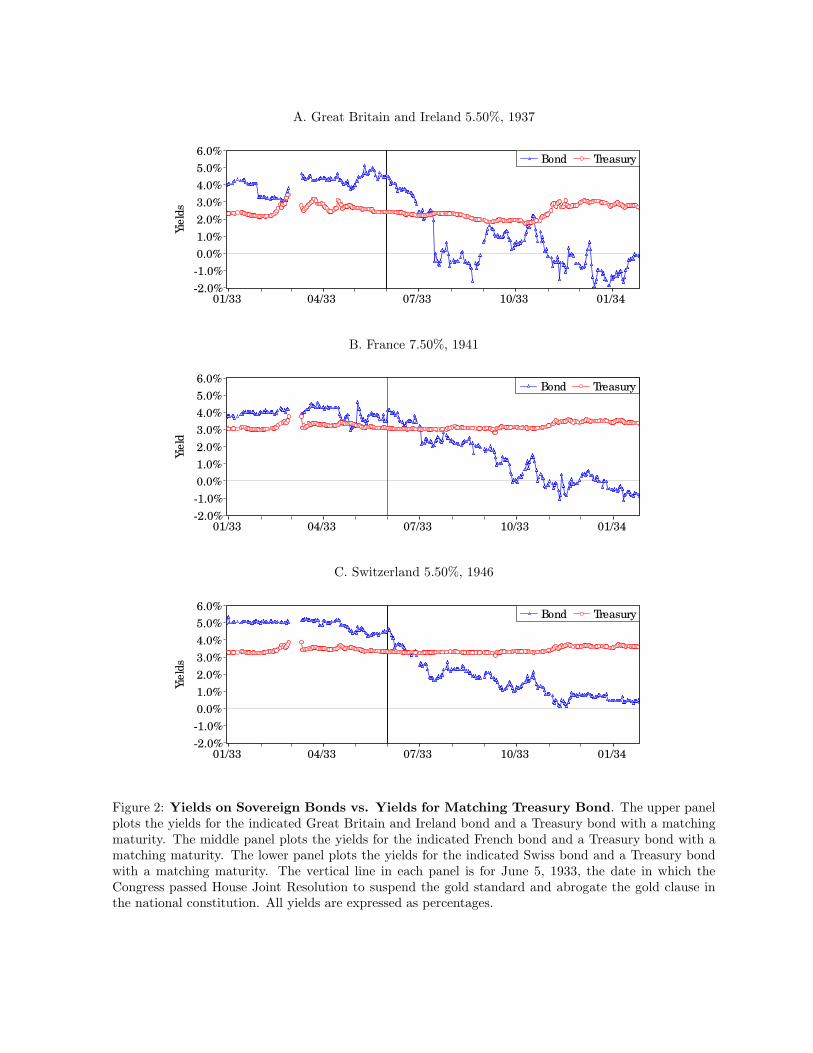
Figure 2 plots the time series of yields for the matched sovereign-Treasury

15The U.K. retained an investment grade rating despite having abandoned thegold standard in 1931. Technically, both the U.K. and France defaulted in 1932on World War I related inter-allied debt owed to the U.S. However, since thepayments on the debt were linked to reparation payments by Germany (whichdefaulted on its obligations in 1931), this has often been viewed as an “excusabledefault.” See Reinhardt and Rogoff (2009).16As will be discussed later, we make the realistic assumption that callable Trea-sury securities will be called at their first call date.

10

pairs of bonds for the period from January 1, 1933, to January 30, 1934 (wefocus on the period prior to the January 31, 1934, official devaluation to avoidconfounding abrogation and devaluation effects). Since the closing prices fromThe New York Times are flat prices, we first add the accrued coupon to theprice of the bond before solving for the yield to maturity. Following standardbond market conventions, the accrued coupon is computed using an actual/actualdaycount basis and the yield to maturity is based on semiannual compoundingbut expressed as an annualized rate. As shown, the yields on the three Treasurysecurities are relatively constant throughout the sample period. Thus, there islittle apparent effect of the abrogation of the gold clause on the level of nominalTreasury yields. In stark contrast, however, Figure 2 also shows that the yieldsof all three sovereign bonds begin to decline precipitously immediately after theabrogation. Within a few months of the abrogation, the yields of the U.K.,French, and Swiss bonds all decline by hundreds of basis points. In each case,the yields on the sovereign bonds quickly approach zero and even attain negativevalues. This common pattern among all three sovereigns has all the hallmarksof a classic flight to quality.

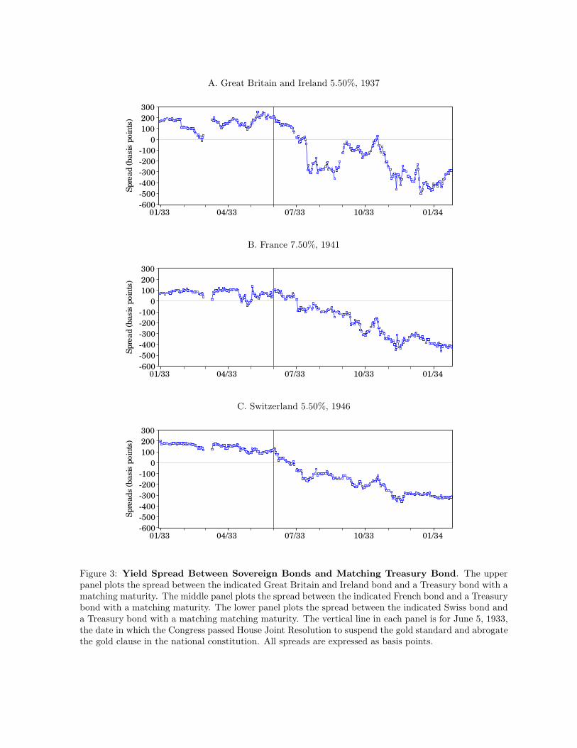
Figure 3 plots the yield spreads between the sovereign bonds and the match-ing Treasury bonds. Table 1 provides summary statistics for these spreads.Specifically, Table 1 reports the mean pre-abrogation spread, the mean post-abrogation spread, and the change in the means, along with the correspondingt-statistics. As shown, the yield spreads for the U.K., French, and Swiss bonds areall significantly positive during the pre-abrogation period, suggesting that theircredit was not viewed as strong as that of the Treasury. After the abrogation,however, the yield spreads all declined very significantly.

These results raise many intriguing research questions. For example, whywere these bonds the focus of an apparent flight to quality? As described above,one possible reason was that these bonds with their Aaa or Aa ratings were amongthe highest-rated sovereign debt issues in the market. A second reason could bethat the fact that these bonds were listed on the New York Stock Exchange mayhave given investors confidence about the ongoing liquidity and tradeability ofthese bonds. On the other hand, the possibility that investors may have believedthat these bonds would be redeemed in gold at ”parity” exchange rates seemsunlikely since the United Kingdom abandoned the gold standard in 1931 andFrance followed suit in 1936. Furthermore, the increases in these bonds’ priceswere larger than could have been explained by the devaluation of the dollar.

11

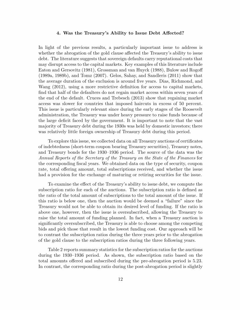
4. Was the Treasury’s Ability to Issue Debt Affected?

In light of the previous results, a particularly important issue to address iswhether the abrogation of the gold clause affected the Treasury’s ability to issuedebt. The literature suggests that sovereign defaults carry reputational costs thatmay disrupt access to the capital markets. Key examples of this literature includeEaton and Gersovitz (1981), Grossman and van Huyck (1988), Bulow and Rogoff(1989a, 1989b), and Tomz (2007). Gelos, Sahay, and Sandleris (2011) show thatthe average duration of the exclusion is around five years. Dias, Richmond, andWang (2012), using a more restrictive definition for access to capital markets,find that half of the defaulters do not regain market access within seven years ofthe end of the default. Cruces and Trebesch (2013) show that regaining marketaccess was slower for countries that imposed haircuts in excess of 50 percent.This issue is particularly relevant since during the early stages of the Rooseveltadministration, the Treasury was under heavy pressure to raise funds because ofthe large deficit faced by the government. It is important to note that the vastmajority of Treasury debt during the 1930s was held by domestic investors; therewas relatively little foreign ownership of Treasury debt during this period.

To explore this issue, we collected data on all Treasury auctions of certificatesof indebtedness (short-term coupon bearing Treasury securities), Treasury notes,and Treasury bonds for the 1930–1936 period. The source of the data was theAnnual Reports of the Secretary of the Treasury on the State of the Finances forthe corresponding fiscal years. We obtained data on the type of security, couponrate, total offering amount, total subscriptions received, and whether the issuehad a provision for the exchange of maturing or retiring securities for the issue.

To examine the effect of the Treasury’s ability to issue debt, we compute thesubscription ratio for each of the auctions. The subscription ratio is defined asthe ratio of the total amount of subscriptions to the total amount of the issue. Ifthis ratio is below one, then the auction would be deemed a “failure” since theTreasury would not be able to obtain its desired level of funding. If the ratio isabove one, however, then the issue is oversubscribed, allowing the Treasury toraise the total amount of funding planned. In fact, when a Treasury auction issignificantly oversubscribed, the Treasury is able to choose among the competingbids and pick those that result in the lowest funding cost. Our approach will beto contrast the subscription ratios during the three years prior to the abrogationof the gold clause to the subscription ratios during the three following years.

Table 2 reports summary statistics for the subscription ratios for the auctionsduring the 1930–1936 period. As shown, the subscription ratio based on thetotal amounts offered and subscribed during the pre-abrogation period is 5.23.In contrast, the corresponding ratio during the post-abrogation period is slightly

12

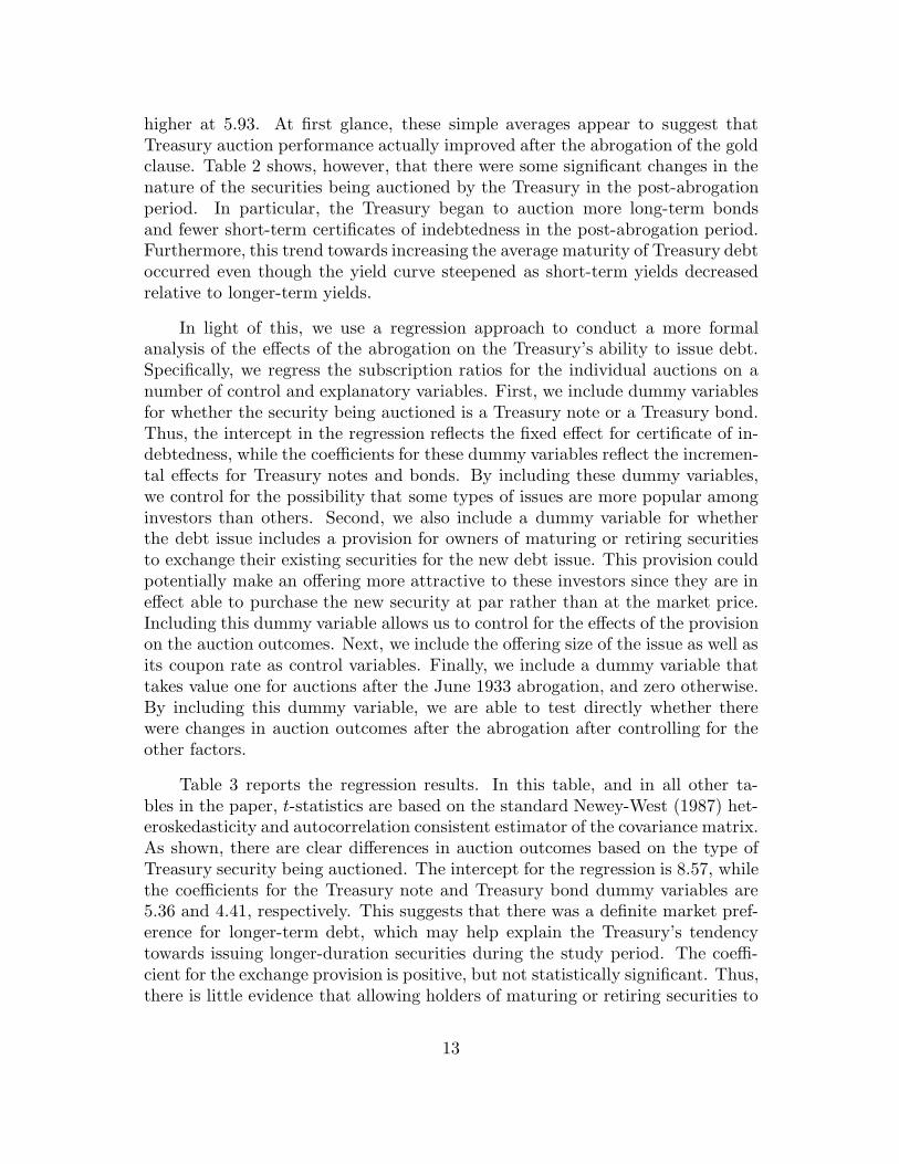
higher at 5.93. At first glance, these simple averages appear to suggest thatTreasury auction performance actually improved after the abrogation of the goldclause. Table 2 shows, however, that there were some significant changes in thenature of the securities being auctioned by the Treasury in the post-abrogationperiod. In particular, the Treasury began to auction more long-term bondsand fewer short-term certificates of indebtedness in the post-abrogation period.Furthermore, this trend towards increasing the average maturity of Treasury debtoccurred even though the yield curve steepened as short-term yields decreasedrelative to longer-term yields.

In light of this, we use a regression approach to conduct a more formalanalysis of the effects of the abrogation on the Treasury’s ability to issue debt.Specifically, we regress the subscription ratios for the individual auctions on anumber of control and explanatory variables. First, we include dummy variablesfor whether the security being auctioned is a Treasury note or a Treasury bond.Thus, the intercept in the regression reflects the fixed effect for certificate of in-debtedness, while the coefficients for these dummy variables reflect the incremen-tal effects for Treasury notes and bonds. By including these dummy variables,we control for the possibility that some types of issues are more popular amonginvestors than others. Second, we also include a dummy variable for whetherthe debt issue includes a provision for owners of maturing or retiring securitiesto exchange their existing securities for the new debt issue. This provision couldpotentially make an offering more attractive to these investors since they are ineffect able to purchase the new security at par rather than at the market price.Including this dummy variable allows us to control for the effects of the provisionon the auction outcomes. Next, we include the offering size of the issue as well asits coupon rate as control variables. Finally, we include a dummy variable thattakes value one for auctions after the June 1933 abrogation, and zero otherwise.By including this dummy variable, we are able to test directly whether therewere changes in auction outcomes after the abrogation after controlling for theother factors.

Table 3 reports the regression results. In this table, and in all other ta-bles in the paper, t-statistics are based on the standard Newey-West (1987) het-eroskedasticity and autocorrelation consistent estimator of the covariance matrix.As shown, there are clear differences in auction outcomes based on the type ofTreasury security being auctioned. The intercept for the regression is 8.57, whilethe coefficients for the Treasury note and Treasury bond dummy variables are5.36 and 4.41, respectively. This suggests that there was a definite market pref-erence for longer-term debt, which may help explain the Treasury’s tendencytowards issuing longer-duration securities during the study period. The coeffi-cient for the exchange provision is positive, but not statistically significant. Thus,there is little evidence that allowing holders of maturing or retiring securities to

13

exchange them for new issues results in better auction outcomes.

The coefficient for the size of the offering is negative and marginally sig-nificant with a t-statistic of −1.95. Intuitively, this result makes sense since itimplies that larger security offerings were more difficult for the market to absorb.This is consistent with the view that there was limited investment capital duringthe Great Depression. In contrast, the coefficient for the coupon rate of the issuebeing auctioned is not significant. This is likely because the Treasury choosesthe coupon rate for the offering to allow the security to be priced at or close topar. Thus, the coupon rate is determined endogenously by the current marketlevel of the term structure.

Focusing now on the key issue of whether the Treasury found it more difficultto issue debt after the abrogation of the gold clause, Table 3 shows that thecoefficient for the post-abrogation dummy variable is negative but not significant.Thus, there is no discernable correlation between the abrogation and auctionoutcomes once the type of debt being issued and the size of the offering arecontrolled for.

These results are consistent with the literature on excusable defaults. Inparticular, Grossman and van Huyck (1988) suggest that some defaults are ex-cusable, and that when that is the case, investors do not punish debtors. Dias,Richmond, and Wang (2012) find that market access occurs faster for defaultersexperiencing a natural disaster; half of them regain access to capital marketswithin three years of the end of default. Edwards (2015a) shows that countriesfacing more severe negative external shocks receive a more favorable treatmentfrom creditors. Finally, Drelichman and Voth (2015) provide historical evidencesupporting the view that excusable defaults do not affect terms or conditions toissue or maintain debt. Our results are consistent with the abrogation of thegold clause having been viewed as an excusable default.

5. Was Treasury Debt Stigmatized?

A separate but related issue is whether the abrogation of the gold clause resultedin infringed holders of gold clause bonds becoming disillusioned and less likelyto own Treasury securities in the future—in other words, stigmatizing Treasurydebt. This issue is closely related to recent research by Guiso, Sapienza, andZingales (2004, 2008), Alesina and Fuchs-Schundeln (2007), Brunnermeier andNagel (2008), Malmendier and Nagel (2011, 2015), and many others who showthat agents’ beliefs and investment decisions depend on their lifetime experiences.

Ideally, we would like to have full information on the portfolio choices of

14

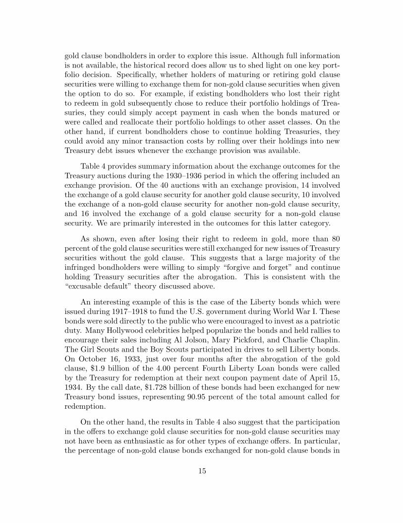
gold clause bondholders in order to explore this issue. Although full informationis not available, the historical record does allow us to shed light on one key port-folio decision. Specifically, whether holders of maturing or retiring gold clausesecurities were willing to exchange them for non-gold clause securities when giventhe option to do so. For example, if existing bondholders who lost their rightto redeem in gold subsequently chose to reduce their portfolio holdings of Trea-suries, they could simply accept payment in cash when the bonds matured orwere called and reallocate their portfolio holdings to other asset classes. On theother hand, if current bondholders chose to continue holding Treasuries, theycould avoid any minor transaction costs by rolling over their holdings into newTreasury debt issues whenever the exchange provision was available.

Table 4 provides summary information about the exchange outcomes for theTreasury auctions during the 1930–1936 period in which the offering included anexchange provision. Of the 40 auctions with an exchange provision, 14 involvedthe exchange of a gold clause security for another gold clause security, 10 involvedthe exchange of a non-gold clause security for another non-gold clause security,and 16 involved the exchange of a gold clause security for a non-gold clausesecurity. We are primarily interested in the outcomes for this latter category.

As shown, even after losing their right to redeem in gold, more than 80percent of the gold clause securities were still exchanged for new issues of Treasurysecurities without the gold clause. This suggests that a large majority of theinfringed bondholders were willing to simply “forgive and forget” and continueholding Treasury securities after the abrogation. This is consistent with the“excusable default” theory discussed above.

An interesting example of this is the case of the Liberty bonds which wereissued during 1917–1918 to fund the U.S. government during World War I. Thesebonds were sold directly to the public who were encouraged to invest as a patrioticduty. Many Hollywood celebrities helped popularize the bonds and held rallies toencourage their sales including Al Jolson, Mary Pickford, and Charlie Chaplin.The Girl Scouts and the Boy Scouts participated in drives to sell Liberty bonds.On October 16, 1933, just over four months after the abrogation of the goldclause, $1.9 billion of the 4.00 percent Fourth Liberty Loan bonds were calledby the Treasury for redemption at their next coupon payment date of April 15,1934. By the call date, $1.728 billion of these bonds had been exchanged for newTreasury bond issues, representing 90.95 percent of the total amount called forredemption.

On the other hand, the results in Table 4 also suggest that the participationin the offers to exchange gold clause securities for non-gold clause securities maynot have been as enthusiastic as for other types of exchange offers. In particular,the percentage of non-gold clause bonds exchanged for non-gold clause bonds in

15

the post-abrogation period was nearly 98 percent. This contrasts, however, withthe percentage for the gold clause for gold clause exchanges in the period priorto the abrogation which was only about 68 percent.

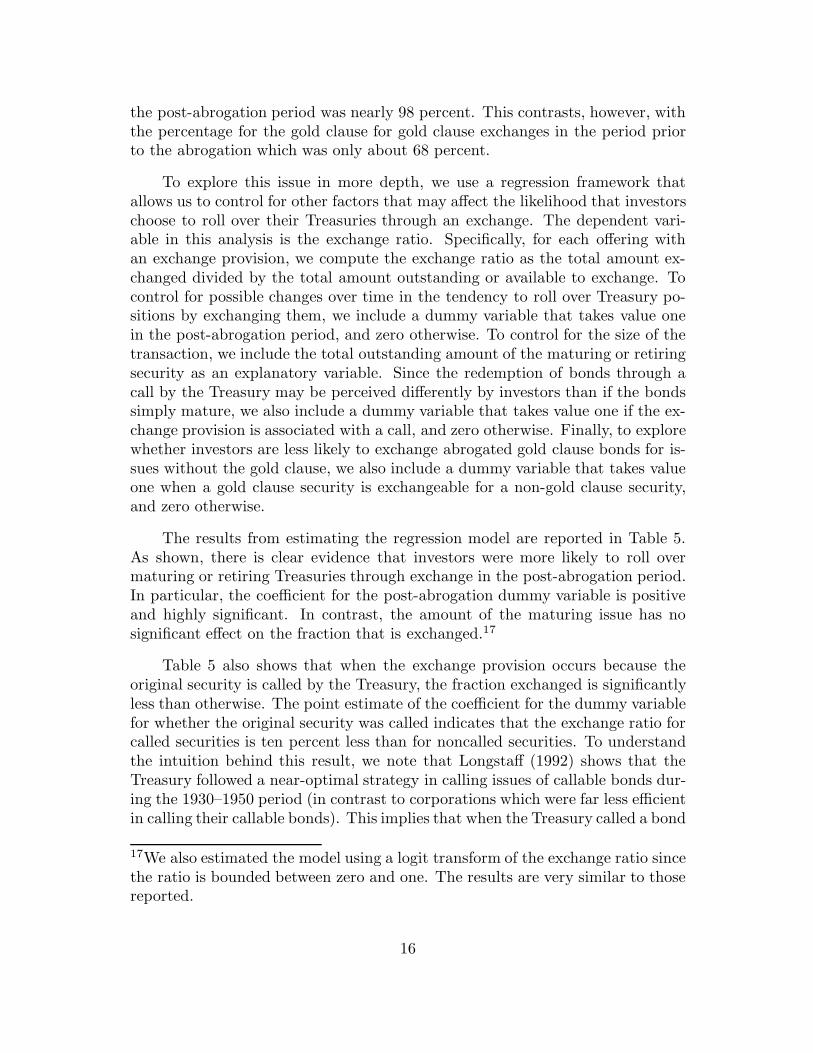
To explore this issue in more depth, we use a regression framework thatallows us to control for other factors that may affect the likelihood that investorschoose to roll over their Treasuries through an exchange. The dependent vari-able in this analysis is the exchange ratio. Specifically, for each offering withan exchange provision, we compute the exchange ratio as the total amount ex-changed divided by the total amount outstanding or available to exchange. Tocontrol for possible changes over time in the tendency to roll over Treasury po-sitions by exchanging them, we include a dummy variable that takes value onein the post-abrogation period, and zero otherwise. To control for the size of thetransaction, we include the total outstanding amount of the maturing or retiringsecurity as an explanatory variable. Since the redemption of bonds through acall by the Treasury may be perceived differently by investors than if the bondssimply mature, we also include a dummy variable that takes value one if the ex-change provision is associated with a call, and zero otherwise. Finally, to explorewhether investors are less likely to exchange abrogated gold clause bonds for is-sues without the gold clause, we also include a dummy variable that takes valueone when a gold clause security is exchangeable for a non-gold clause security,and zero otherwise.

The results from estimating the regression model are reported in Table 5.As shown, there is clear evidence that investors were more likely to roll overmaturing or retiring Treasuries through exchange in the post-abrogation period.In particular, the coefficient for the post-abrogation dummy variable is positiveand highly significant. In contrast, the amount of the maturing issue has nosignificant effect on the fraction that is exchanged.17

Table 5 also shows that when the exchange provision occurs because theoriginal security is called by the Treasury, the fraction exchanged is significantlyless than otherwise. The point estimate of the coefficient for the dummy variablefor whether the original security was called indicates that the exchange ratio forcalled securities is ten percent less than for noncalled securities. To understandthe intuition behind this result, we note that Longstaff (1992) shows that theTreasury followed a near-optimal strategy in calling issues of callable bonds dur-ing the 1930–1950 period (in contrast to corporations which were far less efficientin calling their callable bonds). This implies that when the Treasury called a bond

17We also estimated the model using a logit transform of the exchange ratio sincethe ratio is bounded between zero and one. The results are very similar to thosereported.

16

issue, investors would only have been able to roll over their holdings into bondswith lower coupon rates than the original called bonds. We confirmed this con-jecture by looking at the actual transactions where callable bonds were refundedby new issues. Taken together, these considerations suggest that investors mayhave responded negatively to having their investments in higher coupon bondsterminated by the Treasury by being less willing to roll over called bonds intonew issues with lower coupon rates.

Table 5 shows that a similar effect may be associated with the situationwhere securities with an abrogated gold clause matured or retired and were ex-changeable into a new issue without the gold clause. In particular, the pointestimate for the coefficient for the gold into non-gold dummy variable indicatesthat this situation resulted in an exchange ratio nearly seven percent lower thanotherwise. The coefficient for this dummy variable is also statistically significantas evidenced by its t-statistic of −2.31.

In summary, these results suggest that infringed bondholders responded tothe abrogation of the gold clause by being less willing to exchange their goldclause bonds for non-gold clause bonds. The magnitude of the effect, however,appears to have been relatively modest. For example, based on the coefficientestimates in Table 4 and on the averages for the sample, the effect would be onthe order of reducing the exchange ratio from 89.06 percent to 82.25 percent.This is broadly consistent with the unconditional averages shown in Table 4. Toput these results into perspective, we observe that the effect of the abrogation ofthe gold clause on investors’ willingness to exchange maturing or retiring issuesfor new issues is only about two thirds as large as the effect resulting from bondsbeing called by the Treasury. Despite the fact that a number of bondholders suedthe Treasury because of the abrogation of the gold clause, these results suggestthat little stigma resulted from the abrogation since most investors voluntarilyexchanged their maturing abrogated bonds for new issues without the gold clause.

6. What was the Effect on Treasury Borrowing Costs?

We turn next to the important question of how the abrogation of the gold clausemay have affected the Treasury’s borrowing costs. The literature suggests thatsovereigns with a history of defaults generally are charged higher rates whenthey return to the capital markets. For example, see Lindert and Morton (1989),Flandreau and Zumer (2004), Tomz (2007), and Cruces and Trebesch (2013).

Providing a definitive answer to this issue is challenging for the simple rea-son that there is no direct way of knowing the counterfactual of what Treasuryinterest rates would have been had the gold clause not been abrogated. What we

17

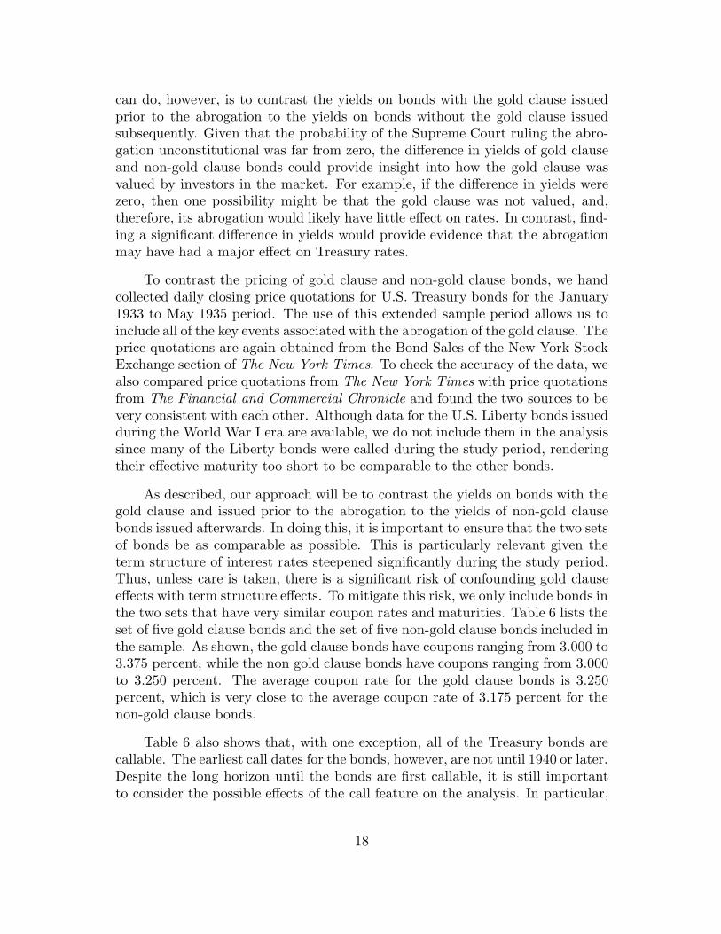
can do, however, is to contrast the yields on bonds with the gold clause issuedprior to the abrogation to the yields on bonds without the gold clause issuedsubsequently. Given that the probability of the Supreme Court ruling the abro-gation unconstitutional was far from zero, the difference in yields of gold clauseand non-gold clause bonds could provide insight into how the gold clause wasvalued by investors in the market. For example, if the difference in yields werezero, then one possibility might be that the gold clause was not valued, and,therefore, its abrogation would likely have little effect on rates. In contrast, find-ing a significant difference in yields would provide evidence that the abrogationmay have had a major effect on Treasury rates.

To contrast the pricing of gold clause and non-gold clause bonds, we handcollected daily closing price quotations for U.S. Treasury bonds for the January1933 to May 1935 period. The use of this extended sample period allows us toinclude all of the key events associated with the abrogation of the gold clause. Theprice quotations are again obtained from the Bond Sales of the New York StockExchange section of The New York Times. To check the accuracy of the data, wealso compared price quotations from The New York Times with price quotationsfrom The Financial and Commercial Chronicle and found the two sources to bevery consistent with each other. Although data for the U.S. Liberty bonds issuedduring the World War I era are available, we do not include them in the analysissince many of the Liberty bonds were called during the study period, renderingtheir effective maturity too short to be comparable to the other bonds.

As described, our approach will be to contrast the yields on bonds with thegold clause and issued prior to the abrogation to the yields of non-gold clausebonds issued afterwards. In doing this, it is important to ensure that the two setsof bonds be as comparable as possible. This is particularly relevant given theterm structure of interest rates steepened significantly during the study period.Thus, unless care is taken, there is a significant risk of confounding gold clauseeffects with term structure effects. To mitigate this risk, we only include bonds inthe two sets that have very similar coupon rates and maturities. Table 6 lists theset of five gold clause bonds and the set of five non-gold clause bonds included inthe sample. As shown, the gold clause bonds have coupons ranging from 3.000 to3.375 percent, while the non gold clause bonds have coupons ranging from 3.000to 3.250 percent. The average coupon rate for the gold clause bonds is 3.250percent, which is very close to the average coupon rate of 3.175 percent for thenon-gold clause bonds.

Table 6 also shows that, with one exception, all of the Treasury bonds arecallable. The earliest call dates for the bonds, however, are not until 1940 or later.Despite the long horizon until the bonds are first callable, it is still importantto consider the possible effects of the call feature on the analysis. In particular,

18

Table 6 shows that the average prices of the callable bonds during the sampleperiod are all significantly above par, implying that the implicit call option isdeep in the money. Given this, we control for the effect of the deep-in-the-moneycall feature on bond prices by assuming the most probable scenario in whichthe call is exercised at the first call date. Accordingly, we compute yields anddurations using the first call date as the effective maturity date.18

Even though Table 6 shows that the two sets of bonds are generally compa-rable in terms of their effective maturity dates, it is clear that there may still beslight differences in average effective maturity across the two sets of bonds. Toaddress this, we construct indexes of the yields for the two sets of bonds in a waythat insures that both indexes are based on portfolios of bonds with identicaldurations. This is done in the following way. Let Yt be the average yield for allof the non-gold clause bonds in the sample at date t. Similarly, let Dt be theaverage duration for these bonds. Now let XLt and DLt be the average yieldand duration, respectively, for the gold clause bonds with durations less thanDt. Let XHt and DHt be the average yield and duration, respectively, for thegold clause bonds with durations greater than or equal to Dt. We then constructthe yield index Xt for the gold clause bonds as the weighted average of XLt andXHt, where the weights are chosen so that the weighted average of DLt and DHt

equals the duration Dt of the non-gold clause bonds. Finally, to guard againstthe potential effects of illiquid bond prices in constructing the yield indexes, in-dex values are only included on days where all five gold clause bonds and allissued non-gold clause bonds have current prices in the New York Times. Theupper panel of Figure 4 plots the time series of the two yield indexes. As shown,the two time series track each other closely throughout the sample period.

Next, we define the gold clause spread as the difference between the yieldindex for non-gold clause bonds and the yield index for gold clause bonds. Giventhis definition, a positive value for the gold clause spread implies that yields ongold clause bonds are lower than those for non-gold clause bonds, or equivalently,that gold clause bonds have higher prices than non-gold clause bonds. The lowerpanel of Figure 4 plots the time series of gold clause spreads.

Table 7 presents summary statistics for the gold clause spread for the entiresample period as well as for four key subperiods. As shown, there is clearly a pos-itive gold clause spread during much of the sample period. This provides supportfor the view that bondholders valued the gold clause, even after it was abrogated.In turn, this suggests that the Treasury did in fact increase its borrowing costs

18This is consistent with the evidence in Longstaff (1992) that the Treasury wasvery efficient in calling its debt optimally. The results are similar when we usethe actual maturity dates for the bonds.

19

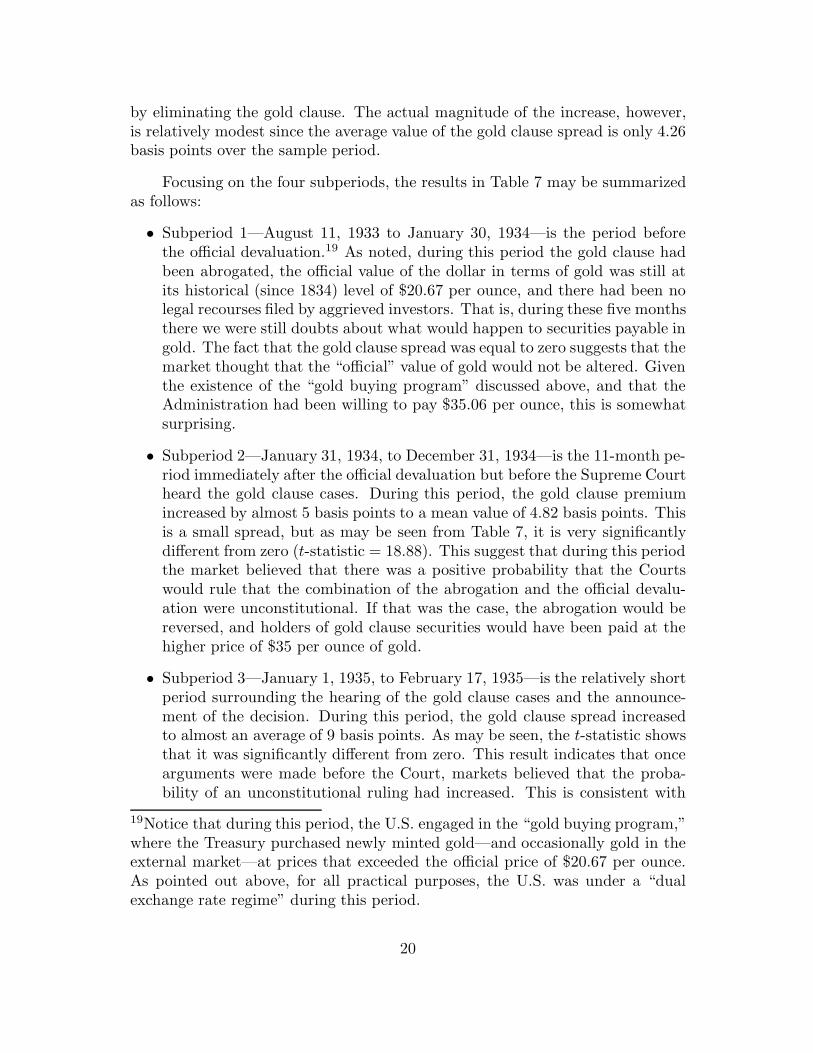
by eliminating the gold clause. The actual magnitude of the increase, however,is relatively modest since the average value of the gold clause spread is only 4.26basis points over the sample period.

Focusing on the four subperiods, the results in Table 7 may be summarizedas follows:

• Subperiod 1—August 11, 1933 to January 30, 1934—is the period beforethe official devaluation.19 As noted, during this period the gold clause hadbeen abrogated, the official value of the dollar in terms of gold was still atits historical (since 1834) level of $20.67 per ounce, and there had been nolegal recourses filed by aggrieved investors. That is, during these five monthsthere we were still doubts about what would happen to securities payable ingold. The fact that the gold clause spread was equal to zero suggests that themarket thought that the “official” value of gold would not be altered. Giventhe existence of the “gold buying program” discussed above, and that theAdministration had been willing to pay $35.06 per ounce, this is somewhatsurprising.

• Subperiod 2—January 31, 1934, to December 31, 1934—is the 11-month pe-riod immediately after the official devaluation but before the Supreme Courtheard the gold clause cases. During this period, the gold clause premiumincreased by almost 5 basis points to a mean value of 4.82 basis points. Thisis a small spread, but as may be seen from Table 7, it is very significantlydifferent from zero (t-statistic = 18.88). This suggest that during this periodthe market believed that there was a positive probability that the Courtswould rule that the combination of the abrogation and the official devalu-ation were unconstitutional. If that was the case, the abrogation would bereversed, and holders of gold clause securities would have been paid at thehigher price of $35 per ounce of gold.

• Subperiod 3—January 1, 1935, to February 17, 1935—is the relatively shortperiod surrounding the hearing of the gold clause cases and the announce-ment of the decision. During this period, the gold clause spread increasedto almost an average of 9 basis points. As may be seen, the t-statistic showsthat it was significantly different from zero. This result indicates that oncearguments were made before the Court, markets believed that the proba-bility of an unconstitutional ruling had increased. This is consistent with

19Notice that during this period, the U.S. engaged in the “gold buying program,”where the Treasury purchased newly minted gold—and occasionally gold in theexternal market—at prices that exceeded the official price of $20.67 per ounce.As pointed out above, for all practical purposes, the U.S. was under a “dualexchange rate regime” during this period.

20

the narrative provided by Meltzer (2003) in his monumental history of theFederal Reserve.

• Subperiod 4—February 18, 1935, to May 31, 1935—begins on the day afterthe Supreme Court ruling that upheld the constitutionality of the JointDeclaration of Congress and goes through May 31, 1945. During this period,the gold clause spread continues to be significantly positive (with a mean of8.43 basis points) and only slightly lower than its mean during subperiod3. Thus, the resolution of uncertainty about the constitutionality of theabrogation had only a small effect on the gold clause spread. Furthermore,we collected additional data on selected dates during the 1935–1938 periodand found that the gold clause spread remained at similar levels over thisextended horizon.

The persistence of the gold clause spread after the Supreme Court decisionsleaves us with an interesting puzzle. Is it possible that investors believed thatthe abrogation of the gold clause and the subsequent devaluation were temporaryand would be reversed when the economic outlook improved? The fact that manyEuropean countries suspended the gold standard during World War I and laterreinstated it during the 1920s provides precedent for the view that the abrogationof the gold clause might only have been temporary. The abrogation of the goldclause could have been reversed, for example, by a new ruling by the SupremeCourt.20

In an effort to shed additional light on this issue, we again use a regressionapproach to examine the factors affecting the gold clause spread. In particular,we regress the spread on several key explanatory variables. The first is theprice of gold as determined in the daily London fixing and reported in The NewYork Times. We include the gold price since it should clearly be an importantdriver of the differential between gold clause and non-gold clause bonds.21 Thevolatility of daily stock market returns is estimated using a Garch(1,1) model.The intuition for including this variable is that stock market volatility reflectsuncertainty about economic fundamentals that could play a role in determininginvestor expectations about a return to the gold standard. The third is a measureof the liquidity of the Treasury security market. Specifically, we compute the ratioof the total daily trading volume of Treasury securities to the total daily trading

20We note that there was precedent for the Supreme Court reversing itself. Forexample, the Supreme Court reversed its earlier decision in Hepburn v. Griswoldin the legal tender or “greenback cases” of 1871, (Knox v. Lee and Parker v.Davis).21Towards the end of the sample period, the price of gold was essentially fixedand the variation in the gold price was minor.

21

volume of all bonds. The data are collected from the New York Times. A declinein this ratio would indicate that the Treasury market is playing a smaller rolein fixed income markets, and vice versa. We also include several lags of the goldclause spread in the regression to control for any persistence in the value of thespread which might affect inferences about the other explanatory variables.

Table 8 reports the regression results. As shown, the first three lags of thegold clause spread are significant, confirming that there is considerable persis-tence in the value of the spread.22 The coefficient for the price of gold is positiveand highly significant. This result is intuitive since the higher the price of gold,the higher is the opportunity cost faced by a bondholder who is not able to re-ceive payment in gold. Thus, this result indicates that the variation in the goldclause spread rationally reflects economic fundamentals.

The coefficient for the volatility of the stock market is negative and signifi-cant. This negative relation is consistent with the interpretation that investorsmay have had ongoing hopes that the gold standard might be reinstated once theeconomic uncertainty associated with the Great Depression was resolved. Thus,when stock market volatility increased, investors’ hopes for a quick return to thegold standard faded, resulting in the decline in the gold clause spread. Finally,the positive and significant coefficient for the Treasury market liquidity factorsuggests that as the Treasury bond market increased in importance, investorsmay have viewed a remediation of the effects of the abrogation as being morelikely, resulting in an increase in the gold clause spread.

These results also shed light on the debate about the effect of the goldstandard on sovereign funding costs. Early studies argued that one of the benefitsof adopting the gold standard is access to cheaper funding, finding yields between30–40 basis points lower for countries that adopted the gold standard during the1870–1914 period (see Bordo and Rockoff (1996) and Obstfeld and Taylor (2003)).More recent evidence, however, challenges these results. Flandreau and Zumer(2004) and Alquist and Chabot (2011) find that there is no relation betweenyields and the gold standard after controlling for differences in monetary andfiscal policies and common risk factors. Our results indicate that bonds with thegold clause had yields that were slightly lower on average than those without thegold clause during the sample period

22Regression specifications including additional lagged values produce resultssimilar to those reported here.

22

7. Conclusion

In this paper we analyze an important, and almost forgotten, episode in U.S. eco-nomic history: the unilateral restructuring of public and private debt contractsby Congress in June 1933. Clauses that linked debt to the price of gold wereannulled in a retroactive fashion. This measure eventually resulted in losses ofthe order of 41 percent.

With few exceptions—the most notable being McCulloch (1980) and Kros-zner (1999)—there has been almost no academic work on the consequences ofthe abrogation of the gold clauses by Congress, and the consequent ratificationof its constitutionality by the Supreme Court in February 1935.

We are particularly interested in investigating the consequences of this gen-eralized breach of contracts. Understanding this issue is not only important toset the historical record straight, but it is also relevant to understand currentevents, and to shed light on the likely consequences of modern defaults, includ-ing debt restructuring in Greece and Argentina. According to traditional theory,after unilaterally restructuring the debt and imposing large losses on investors,debtors should have trouble accessing the capital markets and issuing new debt,the cost of capital should increase significantly, liquidity should be hampered,and there should be a “stigma effect” on new debt. At the aggregate level, a ma-jor credit event and a generalized breach of contracts should result in increaseduncertainty and a reduction in investment and, thus, in a lower growth rate.

Our results show that this episode did not have significant effects on theU.S. Treasury’s ability to roll over maturing debt, or to issue new securities. Wealso find that investors did value the existence of a gold clause in contracts. Sur-prisingly, this gold clause premium continued after the Supreme Court decision,suggesting that the market thought that there was some probability that theSupreme Court would reverse itself at some point in the future. Furthermore, wefind that after Congress abrogated the gold clause, there was a flight to qualityin global financial markets. This was reflected by the fact that the spread offoreign securities over U.S. Treasuries declined significantly.

The results in this paper leave us with some intriguing puzzles. For ex-ample, why did the abrogation of the gold clause have such a small effect onthe Treasury’s ability to issue new bonds or rollover existing debt? Was theabrogation perhaps viewed as an excusable action necessitated by the economiccircumstances? Did the majority of debtholders actually understand that theyhad suffered a loss through the abrogation, or was there some degree of “moneyillusion” involved? The resolution of these puzzles may provide additional usefulinsights into one of the most important episodes in U.S. economic history.

23

References

Acheson, D., 1965. Morning and Noon, New York: Houghton Mifflin.

Alesina, A., and N. Fuchs-Schundeln, 2007. Goodbye Lenin (or Not?): The Effectof Communism on People, American Economic Review 97, 1507-1528.

Alquist, R, and B. Chabot, 2011. Did Gold-Standard Adherence Reduce Sove-reign Capital Costs?, Journal of Monetary Economics 58, 262-272.

Ang, A., and F. A. Longstaff, 2013. Systemic Sovereign Credit Risk: Lessonsfrom the U.S. and Europe, Journal of Monetary Economics 60, 493-510.

Beber, A., M. Brandt, and K. Kavajecz, 2009. Flight-to-Quality or Flight-to-Liquidity? Evidence from the Euro-Area Bond Market, Review of FinancialStudies 22, 925-957.

Benjamin, D, and M. L. J. Wright, 2008. Recovery Before Redemption: ATheory of Delays in Sovereign Debt Renegotiations, Working Paper, Universityof California at Los Angeles.

Bernanke, B., 2000. Essays on the Great Depression, Princeton, NJ: PrincetonUniversity Press.

Bernanke, B., M. Gertler, and S. Gilchrist, 1996. The Financial Accelerator andthe Flight to Quality, The Review of Economics and Statistics 78, 1-15.

Bordo, MD, and H. Rockoff, 1996. The Gold Standard as a “Good HousekeepingSeal of Approval,” Journal of Economic History 56, 389-428.

Borensztein, E., and U. Panizza, 2010. Do Sovereign Defaults Hurt Exporters?Open Economics Review 21, 393-412.

Brunnermeier, M. K. and S. Nagel, 2008. Do Wealth Fluctuations GenerateTime-Varying Risk Aversion? Micro-Evidence on Individuals, American Eco-nomic Review 98, 713-736.

Bulow, J., and K. Rogoff, 1989a. A Constant Recontracting Model of SovereignDebt, Journal of Political Economy 97, 155-178.

Bulow, J., and K. Rogoff, 1989b. Sovereign Debt: Is to Forgive to Forget?,American Economic Review 79, 43-50.

Caballero, R. J., and A. Krishnamurthy, 2008. Collective Risk Management in aFlight to Quality Episode, Journal of Finance 63, 2195-2230.

24

Cruces, J., and C. Trebesch, 2013. Sovereign Defaults: The Price of Haircuts,American Economic Journal: Macroeconomics 5, 85-117.

Dias, D., C. Richmond, and T. Wang, 2012. Duration of Capital Market Exclu-sion: An Empirical Investigation, Working Paper, University of Illinois., Urbana-Champaign.

Drelichman, M. and H.-J. Voth, 2015. Risk Sharing with the Monarch: Contin-gent Debt and Excusable Defaults in the Age of Philip II, 1556-1598, Cliometrica9, 49-75.

Eaton, J., and M. Gersovitz, 1981. Debt with Potential Repudiation: Theoreticaland Empirical Analysis, Review of Economic Studies 48, 289-309.

Eichengreen, B., 1992. Golden Fetters: The Gold Standard and the Great De-pression, 1919–1939, Oxford, UK: Oxford University Press.

Eichengreen, B., G. Hale, and A. Mody, 2001. Flight to Quality: Investor RiskTolerance and the Spread of Emerging Market Crises. In Stijn Claessens andKristin Forbes, eds., International Financial Contagion, Kluwer Academic Pub-lishers.

Edwards, S., 2015a. Sovereign Default, Debt Restructuring, and Recovery Rates:Was the Argentinean “Haircut” Excessive?, Open Economies Review, 1-29.

Edwards, S., 2015b. Academics and Economic Advisors, Gold, the ‘Brains Trust,’and FDR, National Bureau of Economic Research Working Paper No. 21380.

Flandreau, M., and F. Zumer, 2004. The Making of Global Finance 1880-1913,Paris: OECD.

Friedman, M., and A. Schwartz, 1963. A Monetary History of the United States,1867-1960, National Bureau of Economic Research, Inc.

Gelos, R.G., R. Sahay, and G. Sandleris, 2011. Sovereign Borrowing by De-veloping Countries: What Determines Market Access?, Journal of InternationalEconomics 83, 243-254.

Gertler, M., and S. Gilchrist, 1993. The Cyclical Behavior of Short-Term Busi-ness Lending: Implications for Financial Propagation Mechanisms, EuropeanEconomic Review 37, 623-631.

Grossman, H. I., and J. B. Van Huyck, 1988. Sovereign Debt as a ContingentClaim: Excusable Default, Repudiation, and Reputation, American EconomicReview 78, 1088-1097.

Guerrieri, V., and Shimer, R., 2014. Dynamic Adverse Selection: A Theory of

25

Illiquidity, Fire Sales, and Flight to Quality, American Economic Review, 104,1875-1908.

Guiso, L., P. Sapienza, and L. Zingales, 2004. The Role of Social Capital inFinancial Development, American Economic Review 94, 526-556.

Guiso, L., P. Sapienza, and L. Zingales, 2008. Trusting the Stock Market, Journalof Finance 63, 2557-2600.

Kroszner, R.S., 1999. Is It Better to Forgive than to Receive? Repudiation ofthe Gold Indexation Clause in Long-Term Debt During the Great Depression,Unpublished Working Paper, University of Chicago.

Lang, W., and L. Nakamura, 1995. “Flight to Quality” in Banking and EconomicActivity, Journal of Monetary Economics 36, 145-164.

Levy-Yeyati, E., and U. Panizza, 2011. The Elusive Costs of Sovereign Defaults,Journal of Development Economics 94, 95-105.

Lindert P.H., and P.J. Morton, 1989. How Sovereign Debt has Worked. InDeveloping Country Debt and Economic Performance, ed. J. D. Sachs, 39-106,Chicago IL: Univ. Chicago Press.

Longstaff, F. A., 1992. Are Negative Option Prices Possible? The Callable U.S.Treasury-Bond Puzzle, Journal of Business 65, 571-592.

Longstaff, F. A., 2004. The Flight-to-Liquidity Premium in U.S. Treasury BondPrices, Journal of Business 77, 511-526.

MacDonald, J., 2013. A Free Nation Deep in Debt, Princeton, NJ: PrincetonUniversity Press.

Malmendier, U., and S. Nagel, 2011. Depression Babies: Do MacroeconomicExperiences Affect Risk Taking?, The Quarterly Journal of Economics 126, 373-416.

Malmendier, U., and S. Nagel, 2015. Learning from Inflation Experiences, TheQuarterly Journal of Economics, forthcoming.

McCulloch, J. H., 1980. The Ban on Indexed Bonds, 1933-77, American Eco-nomic Review 70, 1018-1021.

Meltzer, Allan H., 2003. A History of the Federal Reserve, Volume 1: 1913-1951,Chicago, IL: The University of Chicago Press, Inc.

Mendoza, E.G., and V.Z. Yue, 2012. A General Equilibrium Model of SovereignDefault and Business Cycles, Quarterly Journal of Economics 127, 889-946.

26

Moley, R., 1939. After Seven Years, New York: Harper and Bros.

Moody’s Investors Service, 1933. Moody’s Manual of Investments, Americanand Foreign, Government Securities, New York NY: Press of Publishers PrintingCompany.

Newey, W. K., and K. D. West, 1987. A Simple Positive Semi-Definite Het-eroskedasticity and Autocorrelation Consistent Covariance Matrix, Econometrica55, 703-708.

Obstfeld, M., and A. M. Taylor, 2003. Sovereign Risk, Credibility and the GoldStandard, 1870-1913 versus 1925-31, Economic Journal 113, 241-275.

Oliner, S. D., and G. D. Rudebusch, 1992. Sources of the Financing Hierarchyfor Business Investment, The Review of Economics and Statistics 74, 643-654.

Pavlova, A., and R. Rigobon, 2008. The Role of Portfolio Constraints in theInternational Propagation of Shocks, Review of Economic Studies 75, 1215-1256.

Reinhart, C. M., and K. S. Rogoff, 2004. Serial Default and the “Paradox” ofRich-to-Poor Capital Flows, American Economic Review 94, 53-58.

Reinhart, C. M., and K. S. Rogoff, 2009. This Time Is Different: Eight Centuriesof Financial Folly, Princeton, NJ: Princeton Univ. Press

Reinhart, C. M., and K. S. Rogoff, 2011. The Forgotten History of DomesticDebt. Economic Journal 121, 319-350.

Roosevelt, F. D., 1938. The Public Papers and Addresses of Franklin D. Roo-sevelt, Volumes 1-5, New York, NY: Random House.

Romer, C. D., 1992. What Ended the Great Depression?, The Journal of Eco-nomic History 52, 757-784.

Rose, A.K., 2005. One Reason Countries Pay their Debts: Renegotiation andInternational Trade, Journal of Development Economics 77, 189-206.

Sturzenegger, F., and J. Zettelmeyer, 2008. Haircuts: Estimating Investor Lossesin Sovereign Debt Restructurings, 1998-2005, Journal of International Moneyand Finance 27, 780-805.

Temin, P., 1991. Lessons from the Great Depression, Boston, MA: MIT PressBooks.

Tomz, M., 2007. Reputation and International Cooperation: Sovereign Debtacross Three Centuries, Princeton, NJ: Princeton University Press.

27

Tomz, M., and M. Wright, 2007. Do Countries Default in “Bad” Times?, Journalof the European Economic Association 5, 352-360.

Tomz, M., and M. Wright, 2013. Empirical Research on Sovereign Debt andDefault, Annual Review of Economics 5, 247-272.

United States Treasury Department, 1921. Liberty Loan Legislation, WashingtonDC: Government Printing Office.

28

2

3

4

5

6

7

8

9

10

21 22 23 24 25 26 27 28 29 30 31 32 33 34 35 36

USD/ Sterling USD/ French Franc

US

D p

er

unit o

f Fore

ign C

urr

ency

Figure 1: U.S. Nominal Exchange Rate. The figure plots the end-of-week nominal exchange ratebetween the U.S. dollar and the Sterling and the French Franc for the period 1921 – 1936. Both ratesare in the form of ”dollars per unit of foreign currency”.

A. Great Britain and Ireland 5.50%, 1937

-2.0%

-1.0%

0.0%

1.0%

2.0%

3.0%

4.0%

5.0%

6.0%

01/33 04/33 07/33 10/33 01/34

Bond Treasury

Yie

lds

B. France 7.50%, 1941

-2.0%

-1.0%

0.0%

1.0%

2.0%

3.0%

4.0%

5.0%

6.0%

01/33 04/33 07/33 10/33 01/34

Bond Treasury

Yie

ld

C. Switzerland 5.50%, 1946

-2.0%

-1.0%

0.0%

1.0%

2.0%

3.0%

4.0%

5.0%

6.0%

01/33 04/33 07/33 10/33 01/34

Bond Treasury

Yie

lds

Figure 2: Yields on Sovereign Bonds vs. Yields for Matching Treasury Bond. The upper panelplots the yields for the indicated Great Britain and Ireland bond and a Treasury bond with a matchingmaturity. The middle panel plots the yields for the indicated French bond and a Treasury bond with amatching maturity. The lower panel plots the yields for the indicated Swiss bond and a Treasury bondwith a matching maturity. The vertical line in each panel is for June 5, 1933, the date in which theCongress passed House Joint Resolution to suspend the gold standard and abrogate the gold clause inthe national constitution. All yields are expressed as percentages.

A. Great Britain and Ireland 5.50%, 1937

-600

-500

-400

-300

-200

-100

0

100

200

300

01/33 04/33 07/33 10/33 01/34

Spre

ad (basi

s poin

ts)

B. France 7.50%, 1941

-600

-500

-400

-300

-200

-100

0

100

200

300

01/33 04/33 07/33 10/33 01/34

Spre

ad (basi

s poin

ts)

C. Switzerland 5.50%, 1946

-600

-500

-400

-300

-200

-100

0

100

200

300

01/33 04/33 07/33 10/33 01/34

Spre

ads

(basi

s poin

ts)

Figure 3: Yield Spread Between Sovereign Bonds and Matching Treasury Bond. The upperpanel plots the spread between the indicated Great Britain and Ireland bond and a Treasury bond with amatching maturity. The middle panel plots the spread between the indicated French bond and a Treasurybond with a matching maturity. The lower panel plots the spread between the indicated Swiss bond anda Treasury bond with a matching matching maturity. The vertical line in each panel is for June 5, 1933,the date in which the Congress passed House Joint Resolution to suspend the gold standard and abrogatethe gold clause in the national constitution. All spreads are expressed as basis points.

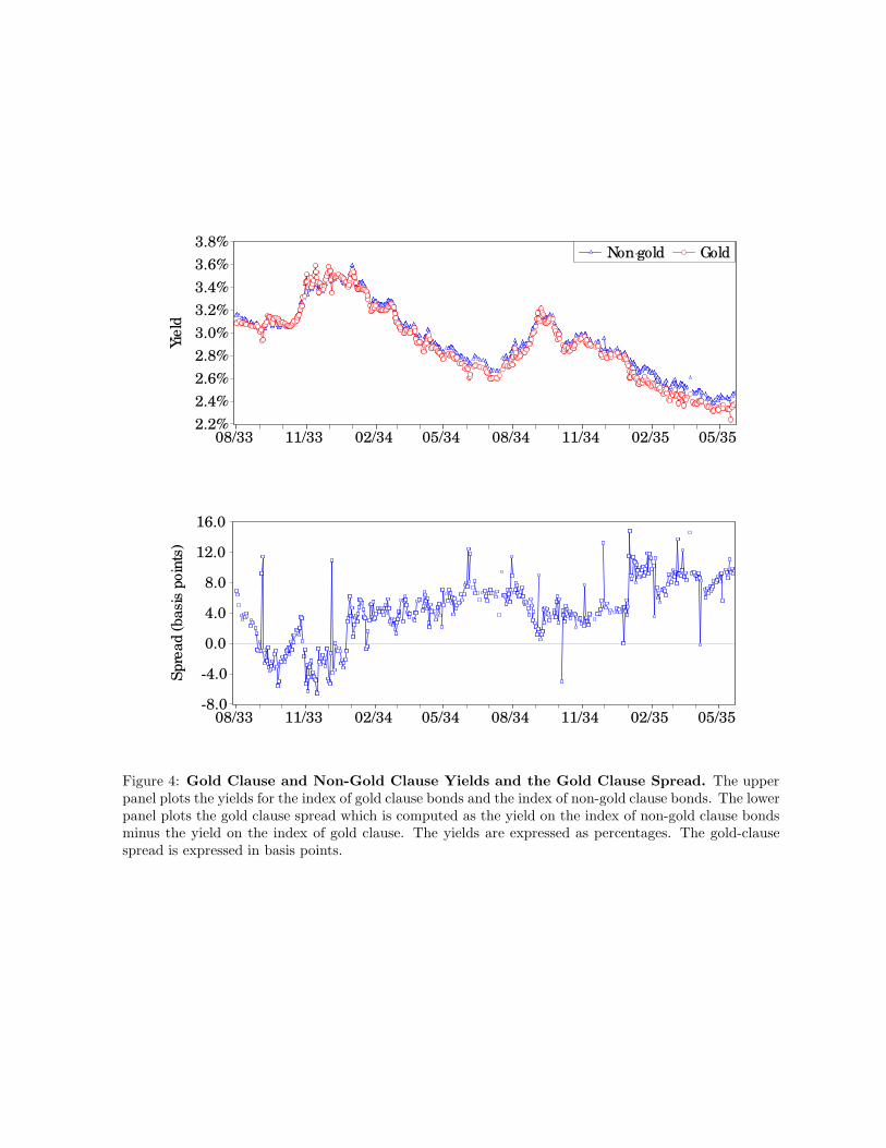
2.2%

2.4%

2.6%

2.8%

3.0%

3.2%

3.4%

3.6%

3.8%

08/33 11/33 02/34 05/34 08/34 11/34 02/35 05/35

Non gold Gold

Yie

ld

−

-8.0

-4.0

0.0

4.0

8.0

12.0

16.0

08/33 11/33 02/34 05/34 08/34 11/34 02/35 05/35

Spre

ad (basi

s poin

ts)

Figure 4: Gold Clause and Non-Gold Clause Yields and the Gold Clause Spread. The upperpanel plots the yields for the index of gold clause bonds and the index of non-gold clause bonds. The lowerpanel plots the gold clause spread which is computed as the yield on the index of non-gold clause bondsminus the yield on the index of gold clause. The yields are expressed as percentages. The gold-clausespread is expressed in basis points.

Table 1

Summary Statistics for Sovereign Minus Treasury Yield Spreads. This table provides summarystatistics for the differences between the yields of the indicated dollar-denominated sovereign bond and amaturity-matched Treasury security. The spreads are measured in basis points. The pre-abrogation period isfrom January 3, 1933 to June 4, 1933. The post-abrogation period is from June 5, 1933 to January 30, 1934.The t-statistics are based on the Newey-West estimator of the covariance matrix. N denotes the number ofobservations.

Sovereign Bond and Period Mean tMean

United Kingdom 5.50% February 1937

Pre-Abrogation 151.17 14.66Post-Abrogation −183.99 −6.29

Change −335.17 −9.98

France 7.50% April 1941

Pre-Abrogation 73.05 11.76Post-Abrogation −209.24 −7.98

Change −282.34 −9.58

Switzerland 5.50% April 1946

Pre-Abrogation 145.32 23.25Post-Abrogation −184.61 −9.48

Change −326.71 −14.72

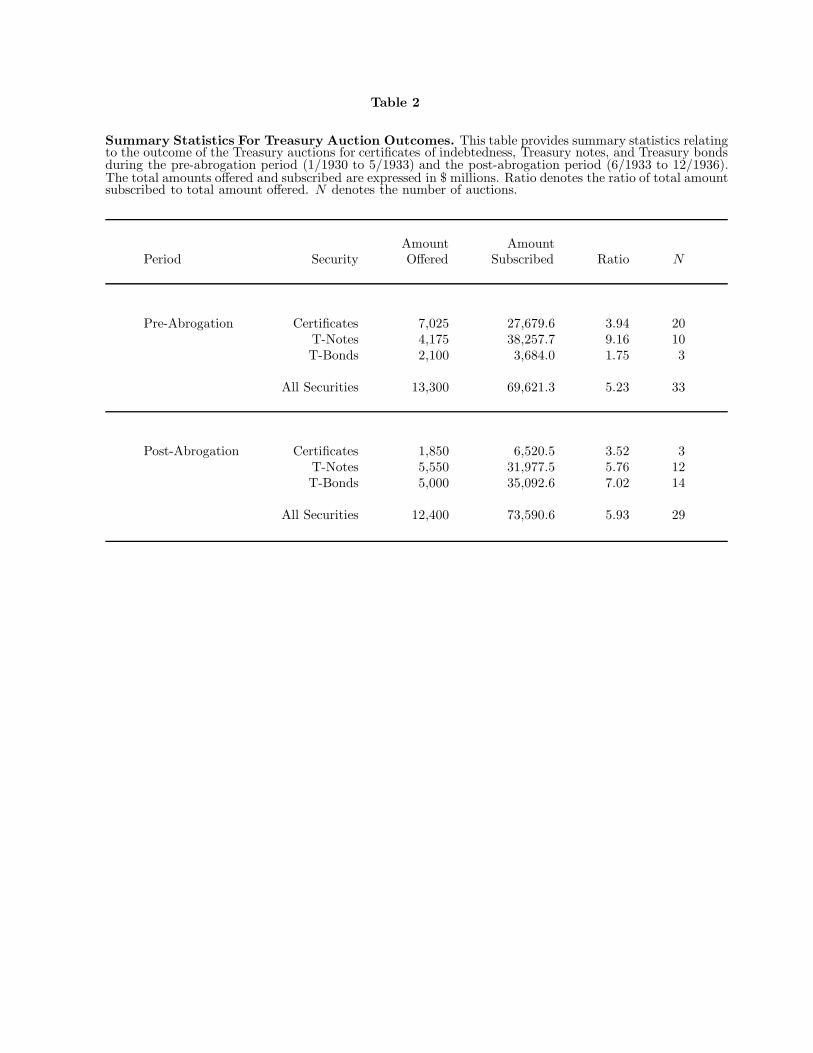
Table 2

Summary Statistics For Treasury Auction Outcomes. This table provides summary statistics relatingto the outcome of the Treasury auctions for certificates of indebtedness, Treasury notes, and Treasury bondsduring the pre-abrogation period (1/1930 to 5/1933) and the post-abrogation period (6/1933 to 12/1936).The total amounts offered and subscribed are expressed in $ millions. Ratio denotes the ratio of total amountsubscribed to total amount offered. N denotes the number of auctions.

Amount AmountPeriod Security Offered Subscribed Ratio N

Pre-Abrogation Certificates 7,025 27,679.6 3.94 20T-Notes 4,175 38,257.7 9.16 10T-Bonds 2,100 3,684.0 1.75 3

All Securities 13,300 69,621.3 5.23 33

Post-Abrogation Certificates 1,850 6,520.5 3.52 3T-Notes 5,550 31,977.5 5.76 12T-Bonds 5,000 35,092.6 7.02 14

All Securities 12,400 73,590.6 5.93 29

Table 3

Results from the Regression of the Subscription Ratio on Explanatory Variables. This tablereports the results from the regression of the subscription ratio (total subscriptions divided by total offeringsize) for the individual Treasury auctions of certificates of indebtedness, Treasury notes, and Treasury bondson the indicated explanatory variables. Treasury Note is a dummy variable that takes value one if theauction is for a Treasury note, and zero otherwise. Treasury bond is a dummy variable that takes value oneif the auction is for a Treasury bond, and zero otherwise. Exchange Provision denotes a dummy variablethat takes value one if the auction includes an exchange provision, and zero otherwise. Issue Size denotesthe offering size of the issue expressed in $millions. Coupon denotes the coupon rate for the issue beingauctioned. Post-Abrogation denotes a dummy variable that takes value one if the auction occurs after theabrogation of the gold clause in June 1933, and zero otherwise. The t-statistics are based on the Newey-West(1980) estimator of the covariance matrix (with three lags). The sample period is 1/1930 to 12/1936.

Variable Coefficient t-Statistic

Intercept 8.5703 2.80Treasury Note 5.3630 1.93Treasury Bond 4.4099 1.86Exchange Provision 2.1175 1.48Issue Size −0.0096 −1.95Coupon −0.9092 −1.12Post-Abrogation −1.8494 −0.75

Adj. R2 0.1538N 62

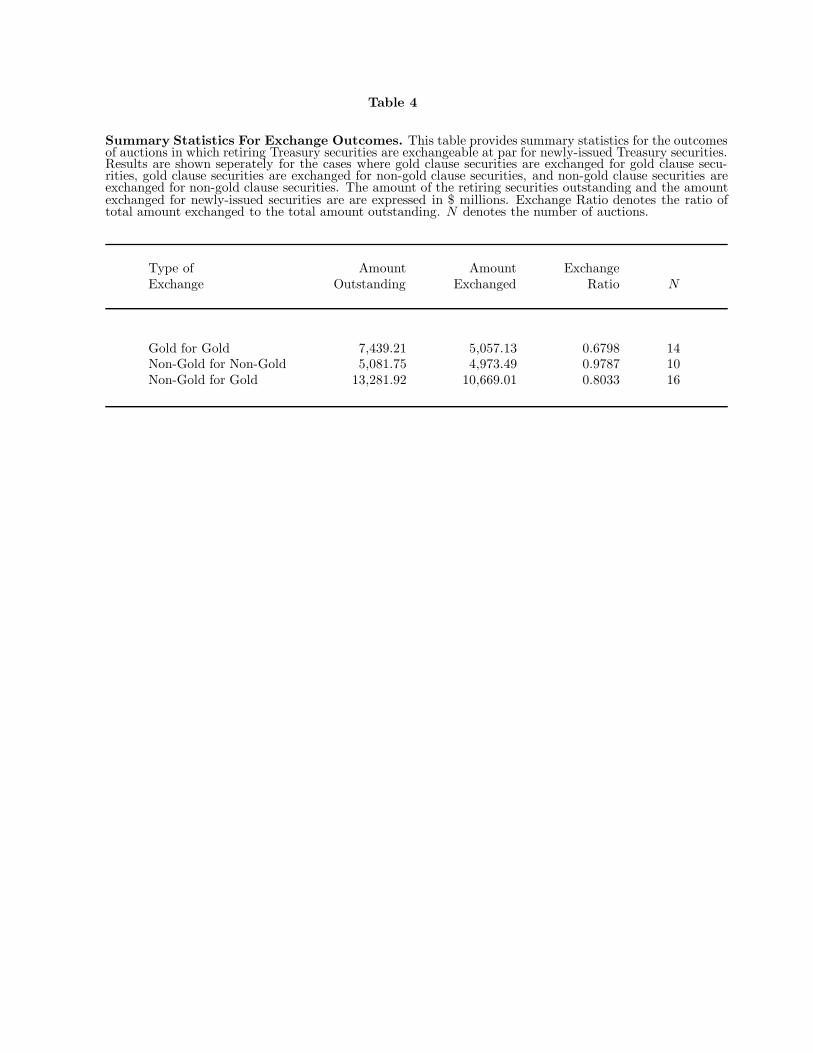
Table 4

Summary Statistics For Exchange Outcomes. This table provides summary statistics for the outcomesof auctions in which retiring Treasury securities are exchangeable at par for newly-issued Treasury securities.Results are shown seperately for the cases where gold clause securities are exchanged for gold clause secu-rities, gold clause securities are exchanged for non-gold clause securities, and non-gold clause securities areexchanged for non-gold clause securities. The amount of the retiring securities outstanding and the amountexchanged for newly-issued securities are are expressed in $ millions. Exchange Ratio denotes the ratio oftotal amount exchanged to the total amount outstanding. N denotes the number of auctions.

Type of Amount Amount ExchangeExchange Outstanding Exchanged Ratio N

Gold for Gold 7,439.21 5,057.13 0.6798 14Non-Gold for Non-Gold 5,081.75 4,973.49 0.9787 10Non-Gold for Gold 13,281.92 10,669.01 0.8033 16

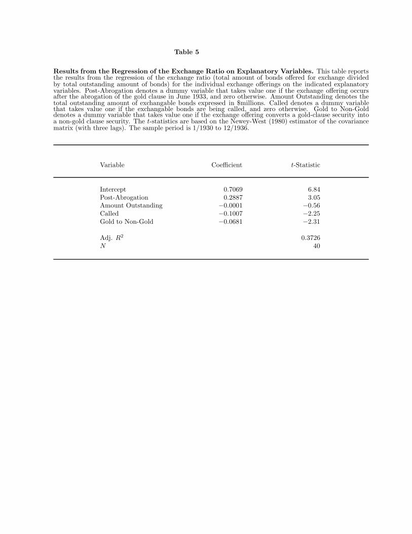
Table 5

Results from the Regression of the Exchange Ratio on Explanatory Variables. This table reportsthe results from the regression of the exchange ratio (total amount of bonds offered for exchange dividedby total outstanding amount of bonds) for the individual exchange offerings on the indicated explanatoryvariables. Post-Abrogation denotes a dummy variable that takes value one if the exchange offering occursafter the abrogation of the gold clause in June 1933, and zero otherwise. Amount Outstanding denotes thetotal outstanding amount of exchangable bonds expressed in $millions. Called denotes a dummy variablethat takes value one if the exchangable bonds are being called, and zero otherwise. Gold to Non-Golddenotes a dummy variable that takes value one if the exchange offering converts a gold-clause security intoa non-gold clause security. The t-statistics are based on the Newey-West (1980) estimator of the covariancematrix (with three lags). The sample period is 1/1930 to 12/1936.

Variable Coefficient t-Statistic

Intercept 0.7069 6.84Post-Abrogation 0.2887 3.05Amount Outstanding −0.0001 −0.56Called −0.1007 −2.25Gold to Non-Gold −0.0681 −2.31

Adj. R2 0.3726N 40

Table 6

Summary Statistics for the U.S. Treasury Bonds. This table reports the average prices, yields, anddurations of the gold clause and non-gold clause bonds in the sample. The bond prices are full prices thatinclude accrued coupon. Yields are expressed as percentages. Duration is expressed in years. N denotes thenumber of daily observations. The sample period is daily from January 1, 1933 to May 31, 1935.

Year of Average Average AverageCoupon Maturity Issuance Price Yield Duration N

Gold Clause Bonds

3.375 Jun 1940-43 1928 103.82 2.823 5.65 6593.375 Mar 1941-43 1931 103.76 2.882 6.24 6603.375 Jun 1943-47 1927 103.60 3.021 7.97 6583.125 Jun 1946-49 1931 101.44 3.057 10.18 6913.000 Sep 1951-55 1931 100.14 3.043 13.61 690

Non-Gold Clause Bonds

3.250 Aug 1941 1933 104.01 2.724 6.36 5233.250∗ Oct 1943-35 1933 103.30 2.981 7.91 4593.250 Apr 1944-46 1934 104.04 2.847 8.17 3293.000 Jun 1946-48 1934 102.33 2.835 9.77 2763.125 Dec 1949-52 1934 104.56 2.806 11.93 131

∗ Coupon is 4.250 until October 1934.

Table 7

Summary Statistics for the Gold-Clause Spread This table reports summary statistics for the gold-clause spread, defined as the difference between the yield on the non-gold-clause bonds and the gold-clausebonds. Spreads are expressed in terms of basis points. The t-statistic for the mean is based on the Newey-West estimator of the variance (with five lags). N denotes the number of daily observations. The sampleperiod is daily from January 1, 1933 to May 31, 1935.

Period From To Mean tMean N

1 11-Aug-1933 30-Jan-1934 −0.04 −0.06 1292 31-Jan-1934 31-Dec-1934 4.82 18.88 2113 1-Jan-1935 17-Feb-1935 8.79 10.50 354 18-Feb-1935 31-May-1935 8.43 23.22 68

Full Sample 11-Aug-1933 31-May-1935 4.26 9.82 443

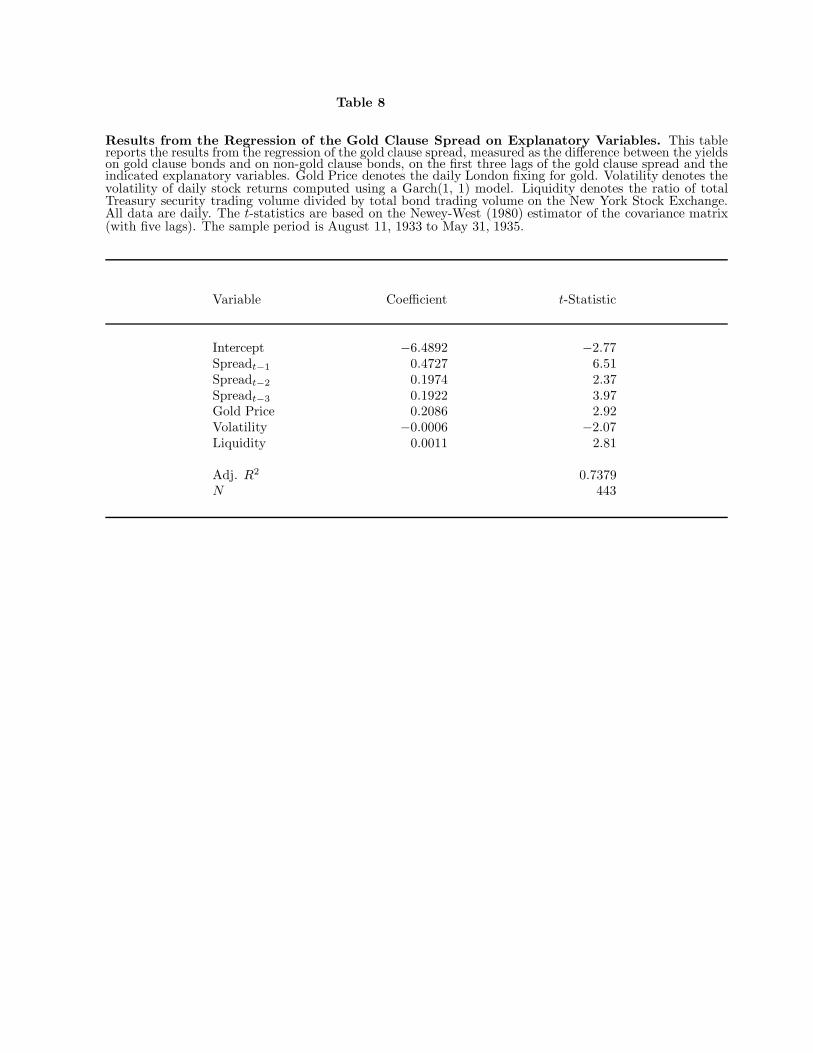
Table 8

Results from the Regression of the Gold Clause Spread on Explanatory Variables. This tablereports the results from the regression of the gold clause spread, measured as the difference between the yieldson gold clause bonds and on non-gold clause bonds, on the first three lags of the gold clause spread and theindicated explanatory variables. Gold Price denotes the daily London fixing for gold. Volatility denotes thevolatility of daily stock returns computed using a Garch(1, 1) model. Liquidity denotes the ratio of totalTreasury security trading volume divided by total bond trading volume on the New York Stock Exchange.All data are daily. The t-statistics are based on the Newey-West (1980) estimator of the covariance matrix(with five lags). The sample period is August 11, 1933 to May 31, 1935.

Variable Coefficient t-Statistic

Intercept −6.4892 −2.77Spreadt−1 0.4727 6.51Spreadt−2 0.1974 2.37Spreadt−3 0.1922 3.97Gold Price 0.2086 2.92Volatility −0.0006 −2.07Liquidity 0.0011 2.81

Adj. R2 0.7379N 443