The Tight Binding Method

Mervyn Roy

May 7, 2015

The tight binding or linear combination of atomic orbitals (LCAO) methodis a semi-empirical method that is primarily used to calculate the bandstructure and single-particle Bloch states of a material. The semi-empiricaltight binding method is simple and computationally very fast. It thereforetends to be used in calculations of very large systems, with more than arounda few thousand atoms in the unit cell.

1 Background: a hierarchy of methods

When the number of atoms and electrons is very small we can use an exactmethod like configuration interaction to calculate the true many-electronwavefunction. However, beyond about 10-electrons we hit the exponentialwall and such calculations become impossible.

For larger systems containing up to a few hundred or a few thousand atomswe can use density functional theory (DFT) techniques to find the trueground state density and ground state energy of the interacting systemwithout explicitly calculating the many-electron wavefunction. In a DFTcalculation we calculate approximate single-particle energies that, in prac-tice, often give a reasonable approximation to the actual band structure ofthe crystal.

In even larger systems, with around 10,000 or more atoms, we can no longeruse self-consistent DFT calculations to take into account the full interaction.To calculate the band structure and a set of approximate single particlestates we instead try to include the effects of the interaction in a semi-empirical way, using parameters that we can adjust to match experiment.

The starting point for all semi-empirical approaches is the physics. In metals,for example, the electrons are almost free and so we can treat the single

1

particle states in terms of plane waves (leading to the Central equation, andnearly free electron theory). We could also take a very different approach andassume the states in a crystal look like combinations of the wavefunctionsof isolated atoms. We might imagine this is more likely to be the case ininsulators or semiconductors.

Here, we will solve the single particle Schrodinger equation for the states ina crystal by expanding the Bloch states in terms of a linear combination ofatomic orbitals.

2 Linear combination of atomic orbitals

2.1 Crystal and atomic hamiltonians

In a crystal, we take the single particle hamiltonian to be

H = Hat + ∆U, (1)

where Hat is the hamiltonian for a single atom and ∆U encodes all thedifferences between the true potential in the crystal and the potential of anisolated atom. We assume ∆U → 0 at the centre of each atom in the crystal.

The single particle states in the crystal are then ψnk(r), where

Hψnk(r) = Enkψnk(r), (2)

the band index is labelled by n, and k is a wavevector in the first Brillouinzone.

2.2 The atomic wavefunctions

The atomic wavefunctions, φi(r) are eigenstates of Hat,

Hatφi(r) = εiφi(r), (3)

where εi is the energy of the i energy level in an isolated atom. Thesewavefunctions decay rapidly away from r = 0 and so the overlap integral,γ(|R|) =

∫φ∗i (r)Hφi(r + R)dr, between wavefunctions located on separate

atomic sites (R 6= 0) in the crystal is small (see Fig. 1).

Throughout these notes we will use orthonormal atomic orbitals that havezero direct overlap between different lattice sites,∫

φ∗i (r)φj(r + R)dr =

{1 if i = j and R = 0

0 otherwise.(4)

2

This gives a simple orthogonal tight-binding formalism but it is relativelyeasy to generalise from this to more complex forms.

0

0.5

1

-1 0 1 2 3 4x (a0)

τ

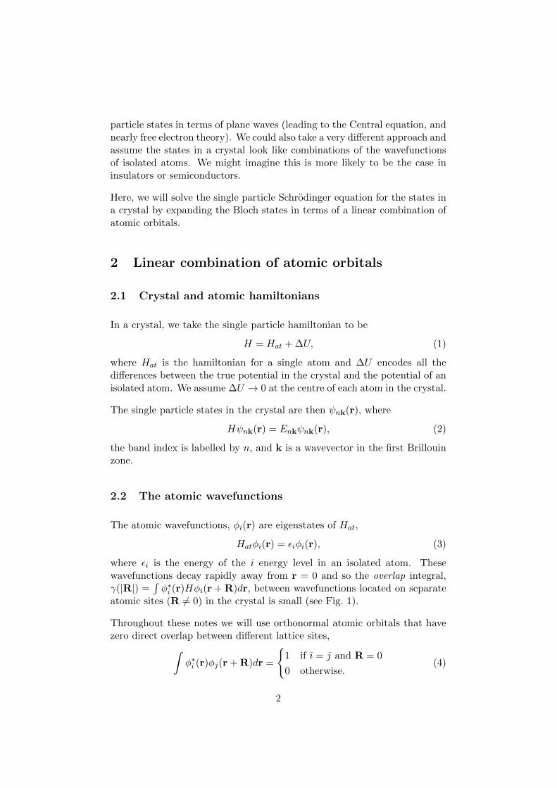
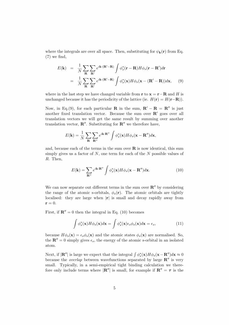
Figure 1: Schematic of the atomic orbitals in a 1D crystal with atoms separated by a0.The translation vectors are R = 0,±a0i,±2a0i,±3a0i, . . ., where i is a unit vector in the xdirection. One of the nearest neighbour vectors τ = a0i is shown in the diagram and thevertical dotted lines denote the edges of the unit cell which contains a single atom. Thesolid curve shows an example atomic orbital centred on an atom at r = 0, while dashedlines show orbitals centred on r+τ and r+ 3τ . The orbitals decay rapidly so the overlap,φ∗i (r)φi(r + R), is small. Here we assume the overlap integral,

∫φ∗i (r)Hφi(r + R)dr, is

only significant when |R| is close to the near-neighbour separation |τ |, and that the directoverlap between orbitals on different lattice sites is zero (see Eq. (4)).

2.3 Bloch’s theorem

The single particle states must obey Bloch’s theorem,

ψnk(r + R) = eik·Rψnk(r), (5)

where R is a real space translation vector of the crystal.

Clearly, a single atomic orbital does not satisfy Bloch’s theorem, but we caneasily make a linear combination of atomic orbitals that does,

ψnk(r) =1√N

∑R

eik·Rφn(r−R), (6)

where there are N lattice sites in the crystal and the factor of 1/√N ensures

the Bloch state is normalised (see appendix A).

3

2.3.1 Proof that∑

R eik·Rφn(r−R) satisfies Bloch’s theorem

If R′ is a real space translation vector and ψnk(r) =∑

R eik·Rφn(r − R)

then,

ψnk(r + R′) =1√N

∑R

eik·Rφn(r− (R−R′)).

But, R−R′ = R′′ is simply another crystal translation vector and, becausethe sum over R goes over all of the translation vectors in the crystal, we canreplace it by another equivalent translation vector, R′′. Then, substitutingfor R = R′ + R′′ in the complex exponential we have

ψnk(r + R′) =1√N

∑R′′

eik·(R′+R′′)φn(r− (R′′)),

= eik·R′ 1√N

∑R′′

eik·R′′φn(r− (R′′)),

= eik·R′ψnk(r),

so that the ψnk(r) =∑

R eik·Rφn(r−R)/

√N from Eq. (6) satisfies Bloch’s

theorem (Eq. (5)).

3 Calculation of the band structure

3.1 Single s-band

Imagine a crystal with translation vectors R, that has one atom in the unitcell, and where only atomic s-orbitals φs(r) contribute to the crystal states.Then there is only 1 band (n = 1) and there is only one Bloch state we canconstruct,

ψk(r) =1√N

∑R

eik·Rφs(r−R). (7)

In this simple case we can find the dispersion relation (the relation betweenenergy and wavevector) simply by calculating the expectation value of theenergy,

E(k) =

∫ψ∗k(r)Hψk(r)dr, (8)

4

where the integrals are over all space. Then, substituting for ψk(r) from Eq.(7) we find,

E(k) =1

N

∑R

∑R′

eik·(R′−R)

∫φ∗s(r−R)Hφs(r−R′)dr

=1

N

∑R

∑R′

eik·(R′−R)

∫φ∗s(x)Hφs(x− (R′ −R))dx, (9)

where in the last step we have changed variable from r to x = r−R and H isunchanged because it has the periodicity of the lattice (ie. H(r) = H(r−R)).

Now, in Eq.(9), for each particular R in the sum, R′ − R = R′′ is justanother fixed translation vector. Because the sum over R′ goes over alltranslation vectors we will get the same result by summing over anothertranslation vector, R′′. Substituting for R′′ we therefore have,

E(k) =1

N

∑R

∑R′′

eik·R′′∫φ∗s(x)Hφs(x−R′′)dx,

and, because each of the terms in the sum over R is now identical, this sumsimply gives us a factor of N , one term for each of the N possible values ofR. Then,

E(k) =∑R′′

eik·R′′∫φ∗s(x)Hφs(x−R′′)dx. (10)

We can now separate out different terms in the sum over R′′ by consideringthe range of the atomic s-orbitals, φs(r). The atomic orbitals are tightlylocalised: they are large when |r| is small and decay rapidly away fromr = 0.

First, if R′′ = 0 then the integral in Eq. (10) becomes∫φ∗s(x)Hφs(x)dx =

∫φ∗s(x)εsφs(x)dx = εs, (11)

because Hφs(x) = εsφs(x) and the atomic states φs(x) are normalised. So,the R′′ = 0 simply gives εs, the energy of the atomic s-orbital in an isolatedatom.

Next, if |R′′| is large we expect that the integral∫φ∗s(x)Hφs(x−R′′)dx ≈ 0

because the overlap between wavefunctions separated by large R′′ is verysmall. Typically, in a semi-empirical tight binding calculation we there-fore only include terms where |R′′| is small, for example if R′′ = τ is the

5

translation vector between an atom and its nearest neighbours (see Fig. 1).Then,

E(k) = εs +∑τ

eik·τ∫φ∗s(x)Hφs(x− τ )dx. (12)

Finally, in an empirical tight binding calculation we do not attempt to evalu-ate the overlap integral,

∫φ∗s(x)Hφs(x−τ )dx explicitly. Instead we replace

it with a parameter, γ, whose value we adjust to match experiment,

γ(|τ |) =

∫φ∗s(x)Hφs(x− τ )dx, (13)

so that,

E(k) = εs +∑τ

eik·τγ(|τ |). (14)

Often empirical relations are also used to scale the overlap integrals with theseparation |τ |. For example, in silicon the relation γ(|τ |) = Ae−α|τ |

2/|τ |2

gives the approximate scaling of the overlap integral with near neighbourseparation |τ |. By using approximate scaling relations, we can investigatethe effect on the band structure of straining or deforming a crystal.

3.2 Single s-band in a 1D crystal

In a 1D crystal the translation vectors are R = na0i where n is an integer,a0 is the atomic separation and i is a unit vector in the x-direction. In thiscase there are two nearest neighbour translation vectors τ = ±a0i.

Then, if ψk(r) =∑

R eik·Rφs(r−R),

E(k) =1

N

∑R

∑R′

eik·(R′−R)

∫φ∗s(r−R)Hφs(r−R′)dr,

=1

N

∑R

∑R′

eik·(R′−R)

∫φ∗s(x)Hφs(x− (R′ −R))dx,

=∑R′′

eik·R′′∫φ∗s(x)Hφs(x−R′′)dx,

= εs +∑τ

eik·τγ(|τ |),

Where we have calculated the expectation value of the energy (line 1)through the following steps,

1. In line 2 we change variable from r to x = r−R.

6

2. In line 3 we replace R′ − R with a translation vector R′′ = R′ − Rthat we can equally well sum over. Once we do this, we recognise thatthe sum over R simply gives a factor of N .

3. Finally, we separate off the R′′ = 0 term (which gives the atomic en-ergy, εs), restrict the remaining terms in the sum to nearest neighboursτ , and replace the overlap integral with some numerical parameter, γ.

In a 1D crystal we know that τ = ±a0i and that the only meaningfulwavevectors, k, must also be in the direction of i, so that k = ki. Then,

E(k) = εs + γ(a0)(eika0 + e−ika0

)= εs + 2γ(a0) cos(ka0). (15)

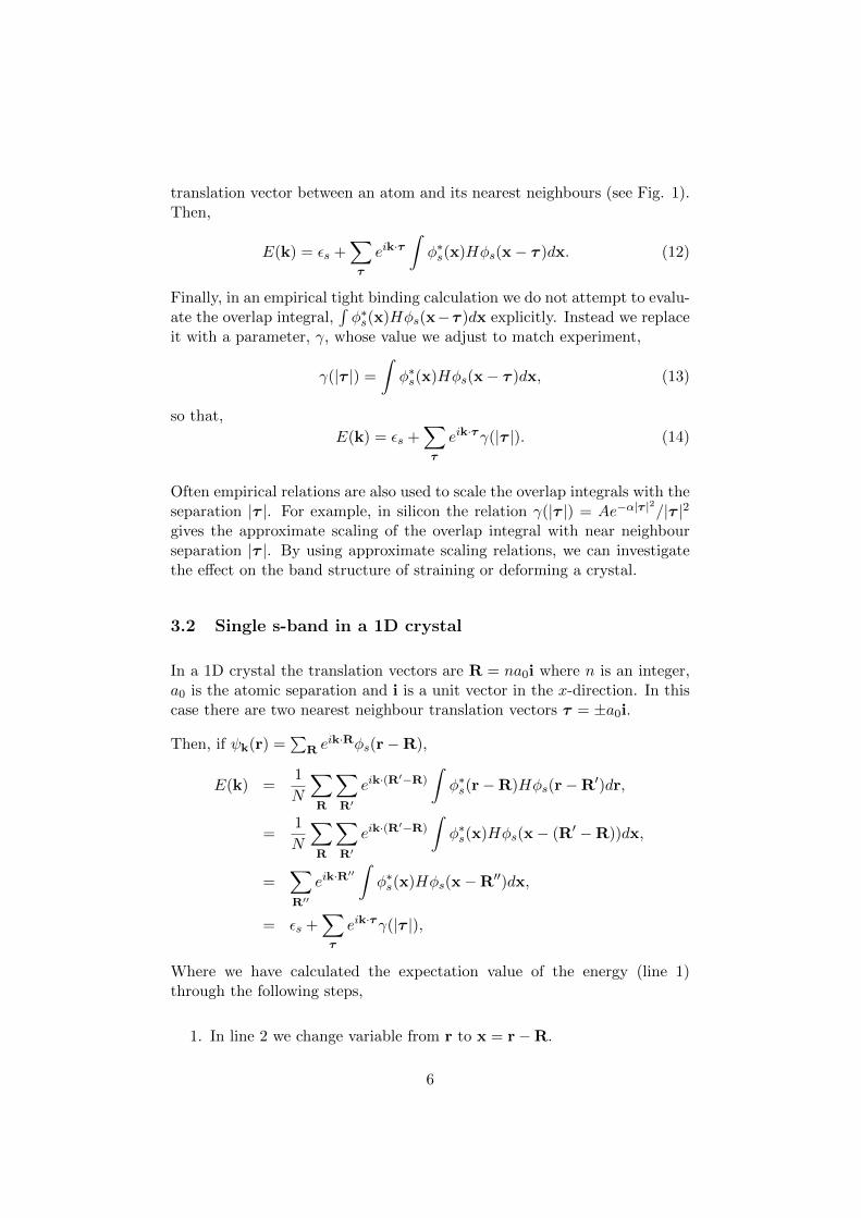
This is the dispersion relation for a single s-band in a 1D crystal. It de-scribes how the energy varies with crystal momentum, k. It also tells us thebandwidth (see Fig. 2).

In the 1D crystal the length of the unit cell in real space is a0, so the lengthof the unit cell in reciprocal space is 2π/a0. In figure 2 we plot E(k) insidethe unit cell in reciprocal space, from k = 0 to k = 2π/a0. At large k thedispersion relation simply repeats.1 The bandwidth, 4γ, is marked on theplot. This is the difference between the maximum and minimum allowedenergy of the band.

εs-2γ

εs

εs+2γ

0 1 2

Energ

y

k (2π/a0)

4γ

Figure 2: The E(k) relationfor a single s-band in a 1Dcrystal. The k range is 0 to2π/a0. The bandwidth 4γ ismarked on the plot.

1Usually we would plot E(k) within the first Brillouin zone (BZ). This is an equivalentcell (the Wigner-Seitz cell) in reciprocal space. The BZ length is still 2π/a0 but the BZextends from −π/a0 to π/a0 rather than 0 to 2π/a0.

7

3.3 s-band in a 2D crystal

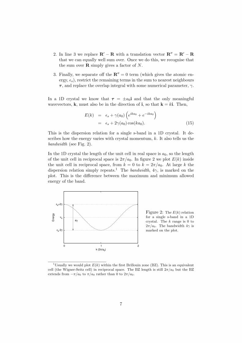
A simple 2D rectangular crystal is shown in Fig. 3 (left). If s-orbitals fromeach atom contribute to the states of the crystal we again have that

E(k) = εs +∑τ

eik·τγ(|τ |),

but now there are 4 vectors: τ = ±ai and τ = ±bj that take us to nearbyatoms where the overlap integral might be significant. The wavevector kcan also vary in both x and y directions, k = kxi + kyj. Then,

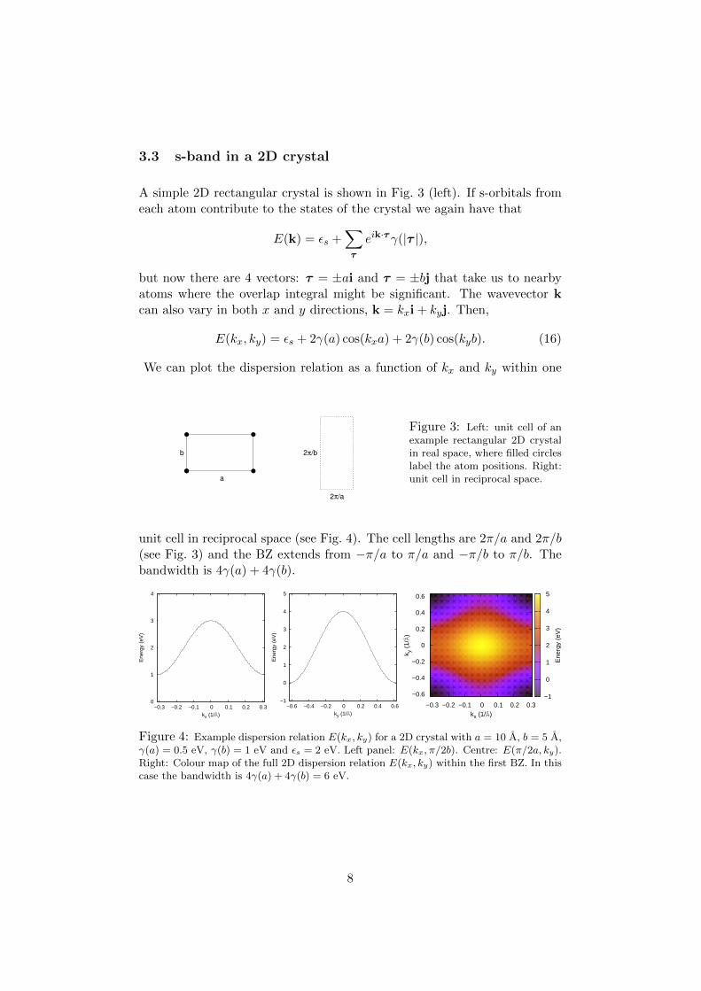
E(kx, ky) = εs + 2γ(a) cos(kxa) + 2γ(b) cos(kyb). (16)

We can plot the dispersion relation as a function of kx and ky within one

a

b

2π/a

2π/b

Figure 3: Left: unit cell of anexample rectangular 2D crystalin real space, where filled circleslabel the atom positions. Right:unit cell in reciprocal space.

unit cell in reciprocal space (see Fig. 4). The cell lengths are 2π/a and 2π/b(see Fig. 3) and the BZ extends from −π/a to π/a and −π/b to π/b. Thebandwidth is 4γ(a) + 4γ(b).

0

1

2

3

4

−0.3 −0.2 −0.1 0 0.1 0.2 0.3

Ene

rgy

(eV

)

kx (1/Å)

−1

0

1

2

3

4

5

−0.6 −0.4 −0.2 0 0.2 0.4 0.6

Ene

rgy

(eV

)

ky (1/Å)

−0.3 −0.2 −0.1 0 0.1 0.2 0.3kx (1/Å)

−0.6

−0.4

−0.2

0

0.2

0.4

0.6

k y (

1/Å

)

−1

0

1

2

3

4

5

Ene

rgy

(eV

)

Figure 4: Example dispersion relation E(kx, ky) for a 2D crystal with a = 10 A, b = 5 A,γ(a) = 0.5 eV, γ(b) = 1 eV and εs = 2 eV. Left panel: E(kx, π/2b). Centre: E(π/2a, ky).Right: Colour map of the full 2D dispersion relation E(kx, ky) within the first BZ. In thiscase the bandwidth is 4γ(a) + 4γ(b) = 6 eV.

8

3.4 s-band in a 3D crystal

Generalising to 3D is now very easy. We still have E(k) = εs+∑

τ eik·τγ(|τ |)

but now k = (kx, ky, kz) and τ will, in general, have x, y, and z components.For example, in a face centred cubic crystal the 12 nearest neighbour vectorsare τ = (±1,±1, 0)a/2, (±1, 0,±1)a/2, (0,±1,±1)a/2. With a little algebrathis eventually gives

E(kx, ky, kz) = εs + 4γ(|τ |)(

coskxa

2cos

kya

2+

coskya

2cos

kza

2+ cos

kza

2cos

kxa

2

), (17)

where |τ | = a/√

2.

3.5 The effect of adjusting the overlap integral, γ.

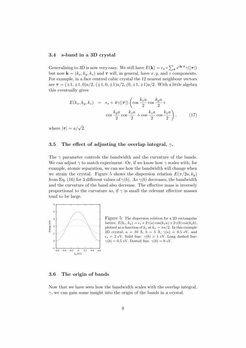
The γ parameter controls the bandwidth and the curvature of the bands.We can adjust γ to match experiment. Or, if we know how γ scales with, forexample, atomic separation, we can see how the bandwidth will change whenwe strain the crystal. Figure 5 shows the dispersion relation E(π/2a, ky)from Eq. (16) for 3 different values of γ(b). As γ(b) decreases, the bandwidthand the curvature of the band also decrease. The effective mass is inverselyproportional to the curvature so, if γ is small the relevant effective massestend to be large.

−1

0

1

2

3

4

5

−0.6 −0.4 −0.2 0 0.2 0.4 0.6

Ene

rgy

(eV

)

ky (1/Å)

Figure 5: The dispersion relation for a 2D rectangularlattice, E(kx, ky) = εs + 2γ(a) cos(kxa) + 2γ(b) cos(kyb),plotted as a function of ky at kx = πa/2. In this example2D crystal, a = 10 A, b = 5 A, γ(a) = 0.5 eV, andεs = 2 eV. Solid line: γ(b) = 1 eV. Long dashed line:γ(b) = 0.5 eV. Dotted line: γ(b) = 0 eV .

3.6 The origin of bands

Now that we have seen how the bandwidth scales with the overlap integral,γ, we can gain some insight into the origin of the bands in a crystal.

9

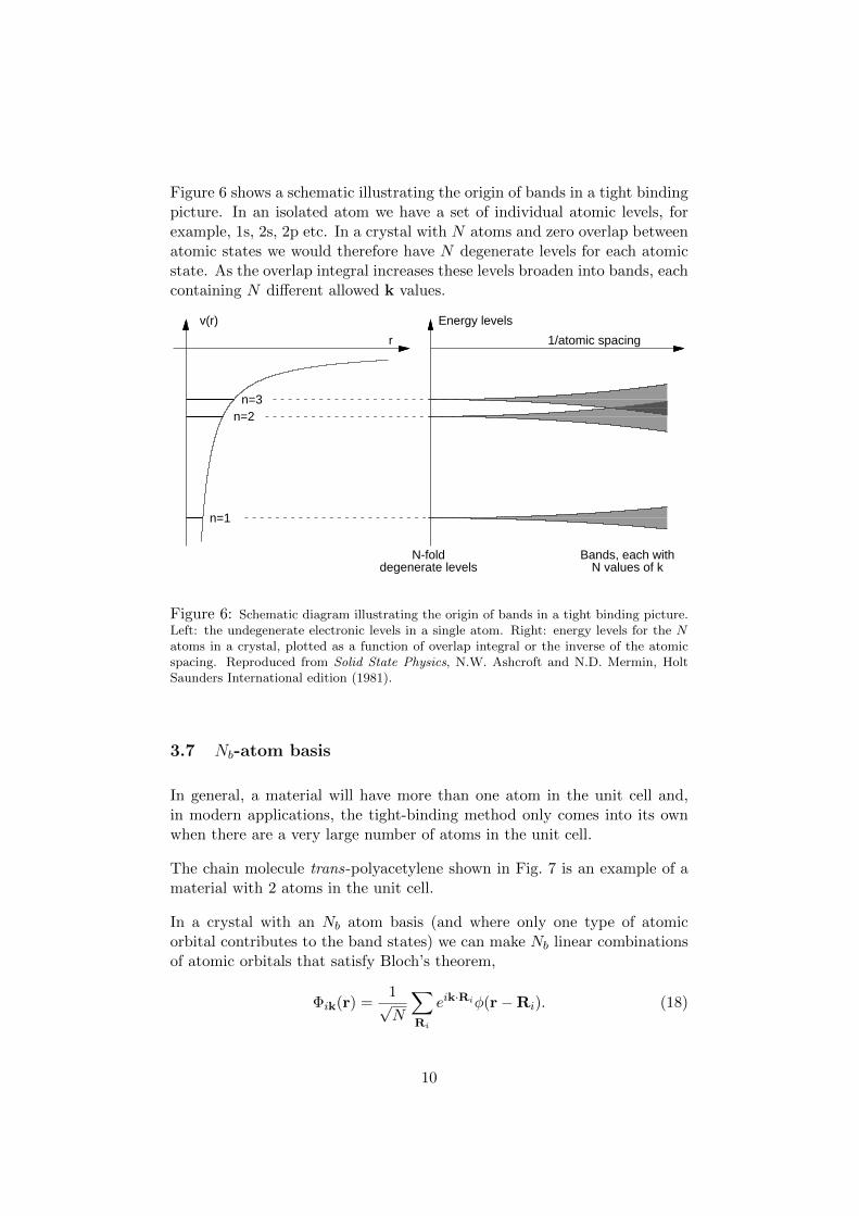
Figure 6 shows a schematic illustrating the origin of bands in a tight bindingpicture. In an isolated atom we have a set of individual atomic levels, forexample, 1s, 2s, 2p etc. In a crystal with N atoms and zero overlap betweenatomic states we would therefore have N degenerate levels for each atomicstate. As the overlap integral increases these levels broaden into bands, eachcontaining N different allowed k values.

r

v(r)

n=1

n=3n=2

1/atomic spacing

Energy levels

N-folddegenerate levels

Bands, each withN values of k

Figure 6: Schematic diagram illustrating the origin of bands in a tight binding picture.Left: the undegenerate electronic levels in a single atom. Right: energy levels for the Natoms in a crystal, plotted as a function of overlap integral or the inverse of the atomicspacing. Reproduced from Solid State Physics, N.W. Ashcroft and N.D. Mermin, HoltSaunders International edition (1981).

3.7 Nb-atom basis

In general, a material will have more than one atom in the unit cell and,in modern applications, the tight-binding method only comes into its ownwhen there are a very large number of atoms in the unit cell.

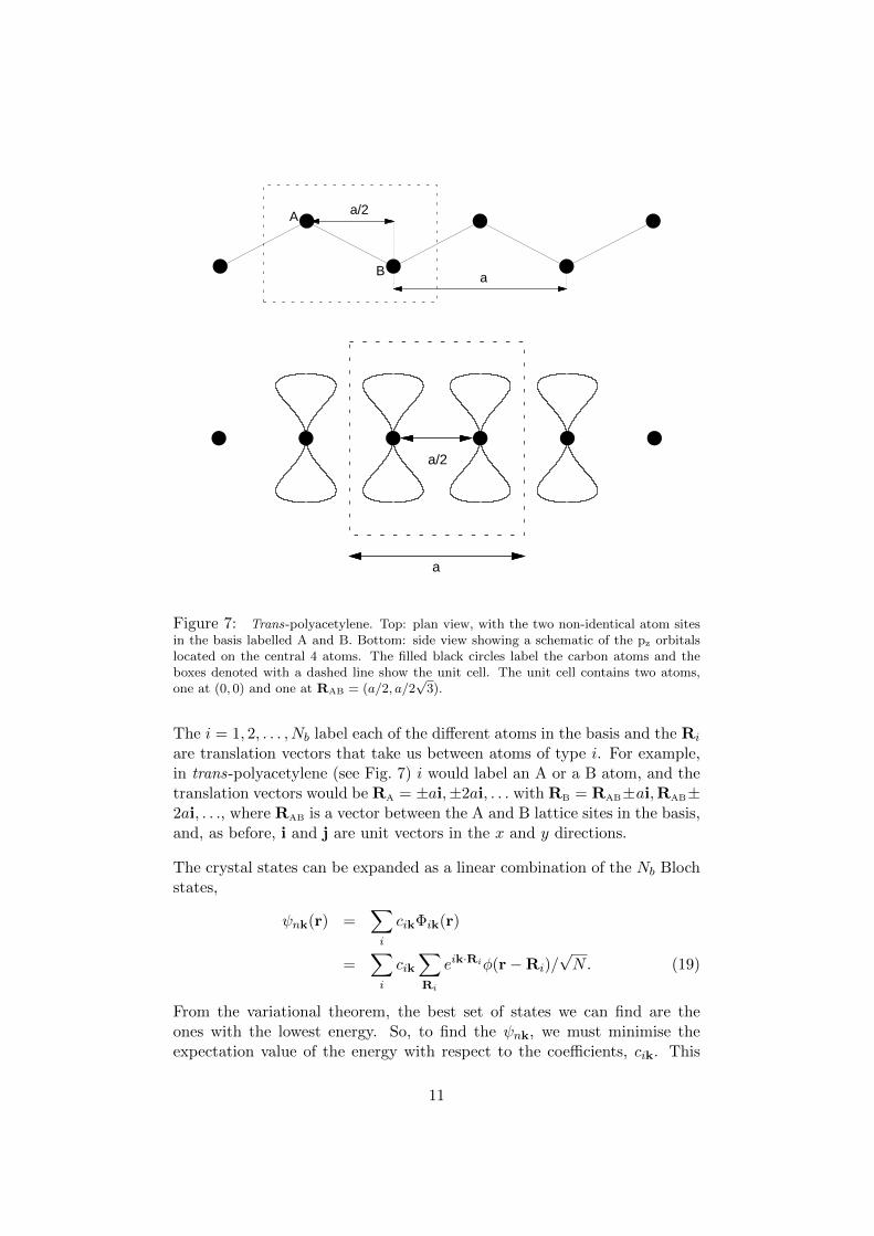
The chain molecule trans-polyacetylene shown in Fig. 7 is an example of amaterial with 2 atoms in the unit cell.

In a crystal with an Nb atom basis (and where only one type of atomicorbital contributes to the band states) we can make Nb linear combinationsof atomic orbitals that satisfy Bloch’s theorem,

Φik(r) =1√N

∑Ri

eik·Riφ(r−Ri). (18)

10

a/2

a

A

B

a/2

a

Figure 7: Trans-polyacetylene. Top: plan view, with the two non-identical atom sitesin the basis labelled A and B. Bottom: side view showing a schematic of the pz orbitalslocated on the central 4 atoms. The filled black circles label the carbon atoms and theboxes denoted with a dashed line show the unit cell. The unit cell contains two atoms,one at (0, 0) and one at RAB = (a/2, a/2

√3).

The i = 1, 2, . . . , Nb label each of the different atoms in the basis and the Ri

are translation vectors that take us between atoms of type i. For example,in trans-polyacetylene (see Fig. 7) i would label an A or a B atom, and thetranslation vectors would be RA = ±ai,±2ai, . . . with RB = RAB±ai,RAB±2ai, . . ., where RAB is a vector between the A and B lattice sites in the basis,and, as before, i and j are unit vectors in the x and y directions.

The crystal states can be expanded as a linear combination of the Nb Blochstates,

ψnk(r) =∑i

cikΦik(r)

=∑i

cik∑Ri

eik·Riφ(r−Ri)/√N. (19)

From the variational theorem, the best set of states we can find are theones with the lowest energy. So, to find the ψnk, we must minimise theexpectation value of the energy with respect to the coefficients, cik. This

11

is a standard procedure (see for example the notes on quantum chemistry)that leads to the following set of simultaneous equations,∑

i

(Hij − δijE(k)) cjk = 0, (20)

where Hij = 〈Φik|H|Φjk〉. This only has non-trivial solutions if the deter-minant,

|H− E(k)I| = 0, (21)

where H is a matrix of elements, Hij , and I is the unit matrix.

3.7.1 2-atom basis

When Nb = 2 the solution of Eq. (21) is simple. We have,∣∣∣∣HAA − E HAB

HBA HBB − E

∣∣∣∣ = 0, (22)

where HAB = H∗BA. This is a simple quadratic equation with two solutions,

E(k) = −1

2(HAA +HBB)±

√1

4(HAA −HBB)2 + |HAB|2. (23)

With two atoms in the unit cell we get 2 valid solutions at each k. Thismeans two bands.

We can calculate the hamiltonian matrix elements in essentially the sameway as we did for the single s-band. For example, in trans-polyacetylene(see Fig. 7) each carbon atom contribute a single p-orbital (of energy ε− p)to the conduction and valence bands. In this case we have,

HAA =1

N

∑RA

∑R′A

eik·(R′A−RA)

∫φ∗s(r−RA)Hφs(r−R′A)dr,

=∑RA′′

eik·R′′A

∫φ∗s(x)Hφs(x−R′′A)dx,

= εp +∑m6=0

eimkaγ(|ma|), (24)

where m is an integer that can be positive or negative, k is the magnitudeof k in the x-direction and, in the last step, we have explicitly substitutedfor the translation vectors RA = mai.

By following the same procedure we can find an identical result for HBB.

12

Next, for simplicity we look at a case where the overlap integrals fall offquickly with distance2, and restrict the overlap integrals to distances ≤ a.Then γ(ma) = 0 for |m| > 1, and we simply have that,

HAA = HBB = εp + 2γ(a) cos(ka). (25)

We follow the same procedure to calculate HAB,

HAB =1

N

∑RA

∑RB

eik·(RA−RB)

∫φ∗s(r−RA)Hφs(r−RB)dr,

=∑RA′

eik·(RAB+R′A)

∫φ∗s(x)Hφs(x− (RAB + R′A))dx. (26)

We include only overlap integrals between nearest neighbours so that weretain only the RA = 0, and RA = −ai terms in the sum (see Fig. 7). Wecan write,

HAB =∑τ

eik·τγ(|τ |), (27)

where, in our case, the nearest neighbour vectors, τ are simply τ = RAB =(a/2, a/2

√3) and τ = RAB − ai = (−a/2, a/2

√3). Again, because trans-

polyacetylene is a one dimensional crystal, k is in the x-direction and,

HAB =(eika/2 + e−ika/2

)γ(|τ |),

= 2 cos(ka/2)γ(|τ |). (28)

Using the results for HAA, HBB, and HAB we can explicitly calculate thedispersion relation from Eq. (23). In trans-polyacetylene,

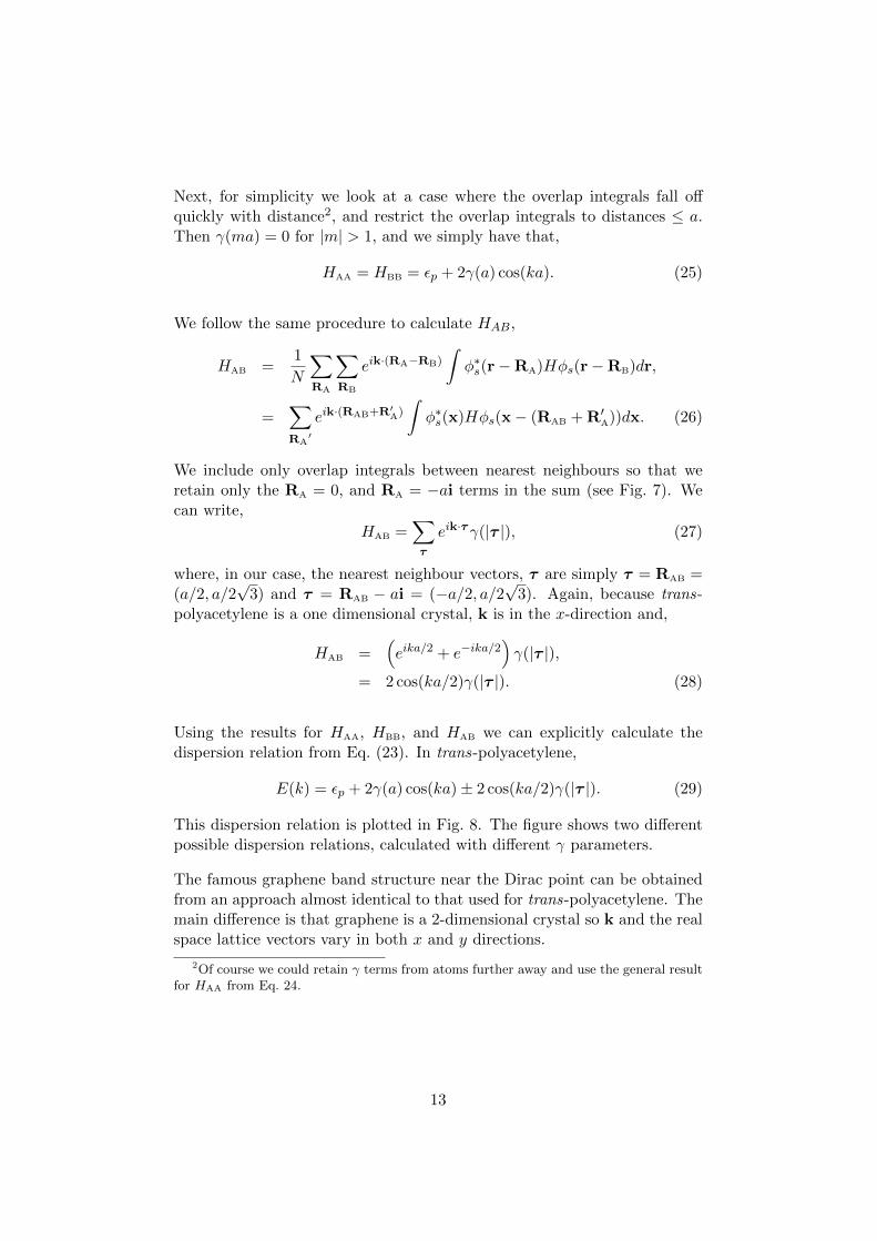
E(k) = εp + 2γ(a) cos(ka)± 2 cos(ka/2)γ(|τ |). (29)

This dispersion relation is plotted in Fig. 8. The figure shows two differentpossible dispersion relations, calculated with different γ parameters.

The famous graphene band structure near the Dirac point can be obtainedfrom an approach almost identical to that used for trans-polyacetylene. Themain difference is that graphene is a 2-dimensional crystal so k and the realspace lattice vectors vary in both x and y directions.

2Of course we could retain γ terms from atoms further away and use the general resultfor HAA from Eq. 24.

13

−1

−0.5

0

0.5

1

1.5

−0.3 −0.2 −0.1 0 0.1 0.2 0.3

Ene

rgy

(eV

)

k (1/Å)

Figure 8: Example dispersion relation(Eq. (29)) for trans-polyacetylene, plottedwithin the first BZ. In this example a =10 A, εp = 0 eV and γ(|τ |) = 0.5 eV.The solid lines show the band structure ina calculation with γ(a) = 0 eV, and thedashed lines show the 2 bands calculatedwith γ(a) = 0.1 eV. In both cases the bandwidth is 4γ(|τ |) = 2 eV.

3.8 Contributions from more than one orbital

In general, bands will contain contributions from more than one type oforbital. In graphene, for example, the lowest energy valence bands (whichform the bonds between atoms) and the highest energy conduction bands,are constructed from a mixture of s, px and py orbitals (this is known as sp2

hybridisation).

However, it is very easy to generalise the formalism in Eq.s (19) and (20) todeal with multiple types of orbital. All we need to do is use the index i tolabel both different basis sites and different orbital types.

For example, imagine a Nb = 2 basis crystal in which s, px, py and pz orbitalsall contribute to the bands of interest. We would then expect 2×4 = 8 bands(from Nb = 2 atoms per unit cell, with 4 orbitals per atom) and we wouldhave to solve an 8×8 matrix eigenvalue equation to find the energies at eachk. In this case, if i = 1 labels an s-orbital on basis site A, and j = 5 labelsa px orbital on basis site B the relevant hamiltonian matrix element wouldbe,

Hij =1

N

∑RA

∑RB

eik·(RA−RB)

∫φ∗s(r−RA)Hφpx(r−RB)dr. (30)

The rest of the hamiltonian matrix elements could be calculated in a similarway and then, as usual, the dispersion relation would be found by solving,

|H− E(k)I| = 0.

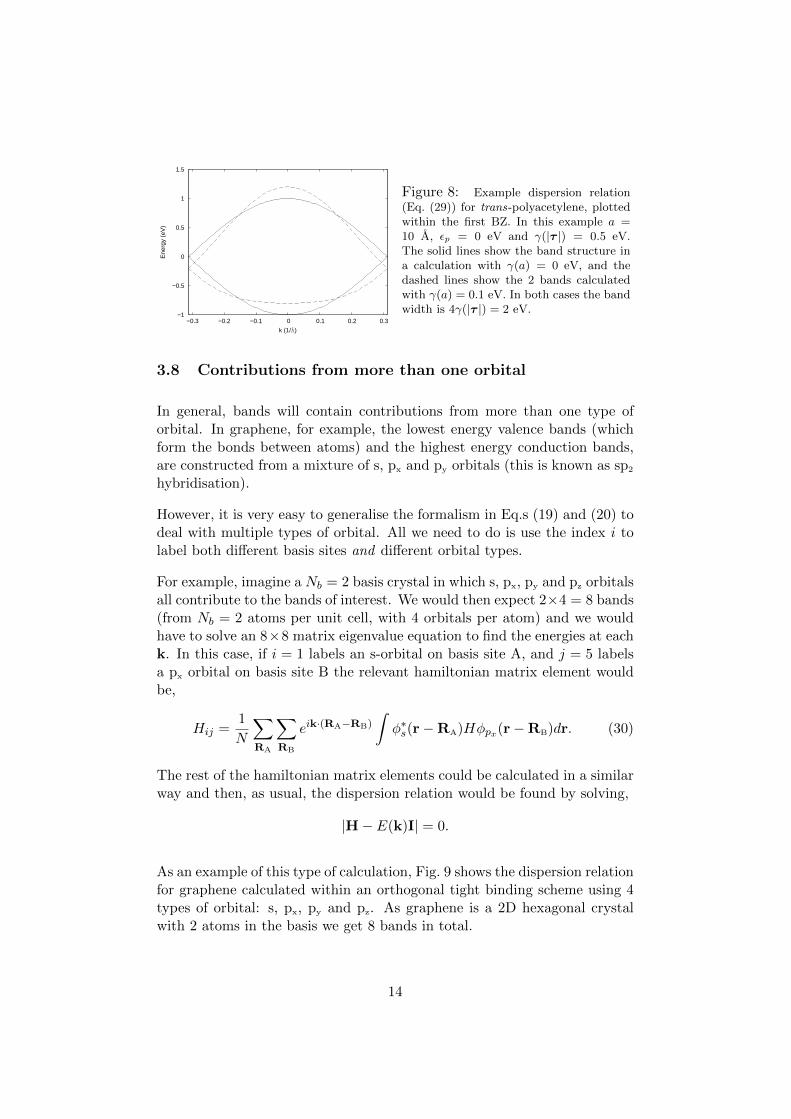
As an example of this type of calculation, Fig. 9 shows the dispersion relationfor graphene calculated within an orthogonal tight binding scheme using 4types of orbital: s, px, py and pz. As graphene is a 2D hexagonal crystalwith 2 atoms in the basis we get 8 bands in total.

14

-30

-25

-20

-15

-10

-5

0

5

10

Γ K Γ X

En

erg

y (

eV

)

wavevector

Figure 9: Calculated E(k) forgraphene using the overlap param-eters of Popov et al Phys. Rev. B70, 115407 (2004). Graphene is a2D crystal with a 2-atom basis inwhich s, px, py and pz orbitals allcontribute to the bands. The pla-nar symmetry means we can sepa-rate the 8× 8 matrix equation into2 matrix equations: a 6 × 6, and a2×2. The s, px and py orbitals mixto form 6 bands (shown in dashedlines). The pz orbitals form theconduction and valence bands atthe Fermi level (solid lines).

A Normalisation of LCAO wavefunction

If, from Eq. (6), our linear combination of atomic orbitals is

ψnk(r) =1√N

∑R

eik·Rφn(r−R),

then the normalisation integral is,

I =

∫ψ∗nk(r)ψnk(r)dr

=1

N

∑R

∑R′

∫e−ik·Rφ∗n(r−R)eik·R

′φn(r−R′)dr

=1

N

∑R

∑R′

eik·(R′−R)

∫φ∗n(r−R)φn(r−R′)dr,

where each of the sums over R and R′ go over the N possible translationvectors in the crystal.

However, from Eq. (4),∫φ∗n(r)φn(r−R)dr = δ(R), where δ(R) is equal to

one if R = 0 and zero otherwise. Hence,

I =1

N

∑R

∑R′

eik·(R′−R)δ(R−R′)

=1

N

∑R

= 1, (31)

and the linear combination of atomic orbitals in Eq. (6) is correctly nor-malised.

15