the suntory and toyota international centres for economics ... · pdf filethe suntory and...

The Suntory and Toyota International Centres for Economics and Related Disciplines

Empirical Tests of Efficiency Wage ModelsAuthor(s): Tzu-Ling Huang, Arne Hallam, Peter F. Orazem, Elizabeth M. PaternoSource: Economica, New Series, Vol. 65, No. 257 (Feb., 1998), pp. 125-143Published by: Blackwell Publishing on behalf of The London School of Economics and Political Scienceand The Suntory and Toyota International Centres for Economics and Related DisciplinesStable URL: http://www.jstor.org/stable/2555133Accessed: 23/09/2010 16:33

Your use of the JSTOR archive indicates your acceptance of JSTOR's Terms and Conditions of Use, available athttp://www.jstor.org/page/info/about/policies/terms.jsp. JSTOR's Terms and Conditions of Use provides, in part, that unlessyou have obtained prior permission, you may not download an entire issue of a journal or multiple copies of articles, and youmay use content in the JSTOR archive only for your personal, non-commercial use.

Please contact the publisher regarding any further use of this work. Publisher contact information may be obtained athttp://www.jstor.org/action/showPublisher?publisherCode=black.

Each copy of any part of a JSTOR transmission must contain the same copyright notice that appears on the screen or printedpage of such transmission.

JSTOR is a not-for-profit service that helps scholars, researchers, and students discover, use, and build upon a wide range ofcontent in a trusted digital archive. We use information technology and tools to increase productivity and facilitate new formsof scholarship. For more information about JSTOR, please contact [email protected].

Blackwell Publishing, The London School of Economics and Political Science, The Suntory and ToyotaInternational Centres for Economics and Related Disciplines are collaborating with JSTOR to digitize,preserve and extend access to Economica.

http://www.jstor.org

http://www.jstor.org/action/showPublisher?publisherCode=black

http://www.jstor.org/action/showPublisher?publisherCode=lonschool

http://www.jstor.org/action/showPublisher?publisherCode=suntoy

http://www.jstor.org/stable/2555133?origin=JSTOR-pdf

http://www.jstor.org/page/info/about/policies/terms.jsp

http://www.jstor.org/action/showPublisher?publisherCode=black

Economica (1998) 65, 125-43

Empirical Tests of Efficiency Wage Models

By TZU-LING HUANG,* ARNE HALLAM,t PETER F. ORAZEMt and ELIZABETH M. PATERNOt

*Ming Chuan University, t Iowa State University

Final version received 29 July 1996.

Two-digit manufacturing industry-level production functions are used to test efficiency wage propositions. Conclusive tests require functional forms which allow differences in elasticities of substitution between observable human capital, wage premia and other inputs. Results demonstrate that unexplained industry wage premia and higher unemployment rates raise productivity. Wage premia and the human capital wage component cannot be aggregated into a single human capital index. Nevertheless, 88% of the productivity effect associated with industry wages can be tied to observable human capital in the industry, with only 12% associated with the wage premium.

INTRODUCTION

Since the publication of Keynes's General Theory, a commonly held view has been that unemployment is caused by stickiness in nominal wages. In fact, both real and nominal wages are quite insensitive to fluctuations in output.' However, economists have failed to reach a consensus on the underlying cause of wage stickiness. A rapidly expanding theoretical literature has attributed wage stickiness and the resulting involuntary unemployment to firms paying efficiency wages to their workers.2 These models hypothesize that worker productivity depends positively on the real wage rate. As a consequence, optimiz- ing firms may not fully adjust real wages, even if output and employment fall.

The main thrust of empirical analysis of efficiency wage models has been to demonstrate that persistent inter-industry wage differentials exist. Krueger and Summers (1988), and Katz and Summers (1989) found industry wage differentials which were uncorrelated with observed measures of human capital, job characteristics, unionization and other individual attributes. Groshen (1991) found unexplained wage differentials across establishments within industries.

Even if persistent unexplained wage differentials exist between establishments or industries, it is unclear if these wage premia are tied to improved productivity. Direct studies of this sort have concentrated on lesser developed economies where worker nutrition is affected by wage levels; for example, Strauss (1986) found a strong direct effect between caloric intake and farm labour productivity in Sierra Leone. In developed industrial economies, nutrition is unlikely to be affected by marginal changes in wages. In developed economy contexts, wage increases are assumed to alter productivity by lowering the incentives for workers to quit, improving worker morale, or lowering incentives to shirk.

Recently, several papers have attempted to establish whether paying wages above the market does indeed raise worker productivity. Cappelli and Chauvin (1991) studied layoffs in a large, multiplant firm with broadly dispersed plants. Increasing plant wages relative to local wages had a negative effect on the ? The London School of Economics and Political Science 1998

126 ECONOMICA [FEBRUARY

annual rate of disciplinary layoffs. They attribute this result to a negative effect of relative wages on incentives to shirk. Using a sample of 219 UK manufacturing companies, Wadhwani and Wall (1991) found that increasing firm wages relative to wages in the industry had a positive effect on firm sales. Using a sample of business units of large US manufacturing corporations, Levine (1992) found that increasing firm wages relative to wages of the firm's nearest three competitors increased output.

This study extends the existing literature in several ways. First, we test whether effects consistent with efficiency wages can be observed at the two- digit industry level rather than at the firm level. This is useful for two reasons. First, it avoids the problem that the firm-level studies have been based on nonrandom samples of firms. It is possible that positive correlation between high wages and output are related to the sample selection process rather than a true productivity effect.3 A similar finding across all manufacturing firms would diffuse the selection bias criticism. Second, most of the studies reporting persistent unexplained wage differentials have concentrated on differences across industries, but productivity studies have concentrated on differences across firms within industries. This study explores whether unexplained wage differentials across industries are related to differences in labour productivity across industries.

Krueger and Summers and Katz and Summers used Mincer-type earnings functions to derive their estimates of efficiency wages. A comparable method- ology is employed in this study to decompose industry-level wages into two portions, one attributable to observable human capital and another orthogonal to observable human capital. Cappelli and Chauvin, Wadhwani and Wall, and Levine all used a single observed relative wage as their measure of the efficiency wage, which confuses human capital with wage premia.

The final innovation in this study is the use of flexible forms rather than the modified Cobb-Douglas specifications employed in earlier studies.4 It turns out that observed and unobserved human capital components of the wage have virtually identical output elasticities so that a Cobb-Douglas form cannot reject the hypothesis that observed and unobserved components of the wage are the same input. The main advantage of the flexible form is that it allows inputs to be complements as well as substitutes in production, a feature that proves critical in demonstrating that the observed human capital component and the wage premium are distinct inputs. The two components can be dis- tinguished by their sharply differing elasticities of substitution with numbers of workers and with physical capital, and the data strongly reject the hypothesis that the two components can be aggregated into a single human capital index.

The wage premium behaves like efficiency wages in theories advanced by Solow (1979) and Shapiro and Stiglitz (1984). Nevertheless, this does not guarantee that the unexplained portion of the wage is an efficiency wage, since the unexplained wage differential could still be due to unmeasured human capital. For example, Murphy and Topel (1990) have argued that positive correlation between unobserved and observed ability would lead to higher unobserved human capital in high-wage industries. Our findings do show, however, that, if the unexplained wage component is unobserved human capital, then observed and unobserved human capital are markedly different inputs. ? The London School of Economics and Political Science 1998

1998] EMPIRICAL TESTS OF EFFICIENCY WAGE MODELS 127

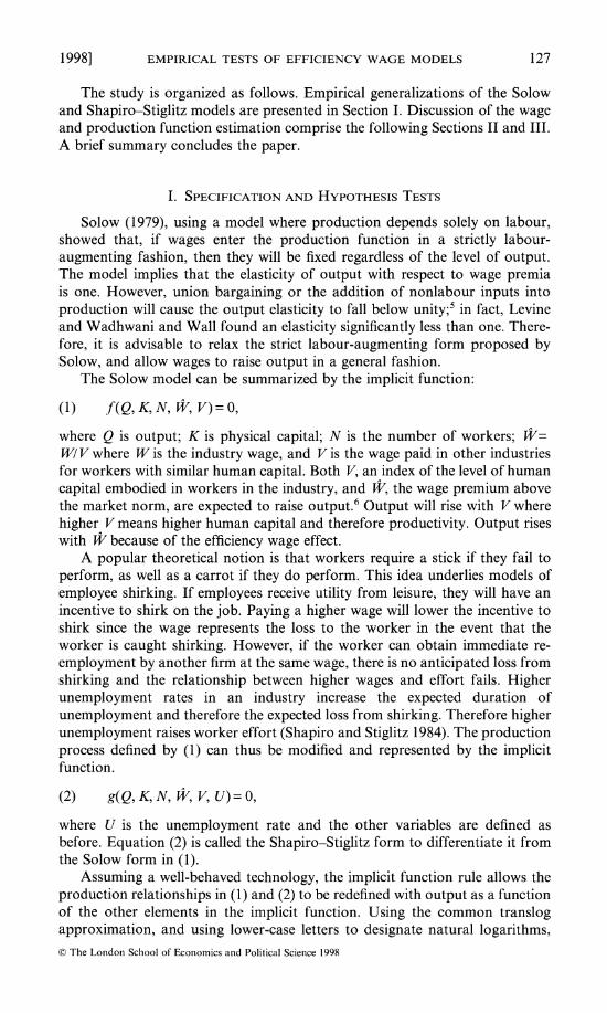
The study is organized as follows. Empirical generalizations of the Solow and Shapiro-Stiglitz models are presented in Section I. Discussion of the wage and production function estimation comprise the following Sections II and III. A brief summary concludes the paper.

I. SPECIFICATION AND HYPOTHESIS TESTS

Solow (1979), using a model where production depends solely on labour, showed that, if wages enter the production function in a strictly labour- augmenting fashion, then they will be fixed regardless of the level of output. The model implies that the elasticity of output with respect to wage premia is one. However, union bargaining or the addition of nonlabour inputs into production will cause the output elasticity to fall below unity;5 in fact, Levine and Wadhwani and Wall found an elasticity significantly less than one. There- fore, it is advisable to relax the strict labour-augmenting form proposed by Solow, and allow wages to raise output in a general fashion.

The Solow model can be summarized by the implicit function:

(1) f(Q,K,N, W, V)=O,

where Q is output; K is physical capital; N is the number of workers; W= WI V where W is the industry wage, and V is the wage paid in other industries for workers with similar human capital. Both V, an index of the level of human capital embodied in workers in the industry, and W, the wage premium above the market norm, are expected to raise output.6 Output will rise with V where higher V means higher human capital and therefore productivity. Output rises with W because of the efficiency wage effect.

A popular theoretical notion is that workers require a stick if they fail to perform, as well as a carrot if they do perform. This idea underlies models of employee shirking. If employees receive utility from leisure, they will have an incentive to shirk on the job. Paying a higher wage will lower the incentive to shirk since the wage represents the loss to the worker in the event that the worker is caught shirking. However, if the worker can obtain immediate re- employment by another firm at the same wage, there is no anticipated loss from shirking and the relationship between higher wages and effort fails. Higher unemployment rates in an industry increase the expected duration of unemployment and therefore the expected loss from shirking. Therefore higher unemployment raises worker effort (Shapiro and Stiglitz 1984). The production process defined by (1) can thus be modified and represented by the implicit function.

(2) g(Q,K,N, W, V, U)=O,

where U is the unemployment rate and the other variables are defined as before. Equation (2) is called the Shapiro-Stiglitz form to differentiate it from the Solow form in (1).

Assuming a well-behaved technology, the implicit function rule allows the production relationships in (1) and (2) to be redefined with output as a function of the other elements in the implicit function. Using the common translog approximation, and using lower-case letters to designate natural logarithms, ? The London School of Economics and Political Science 1998


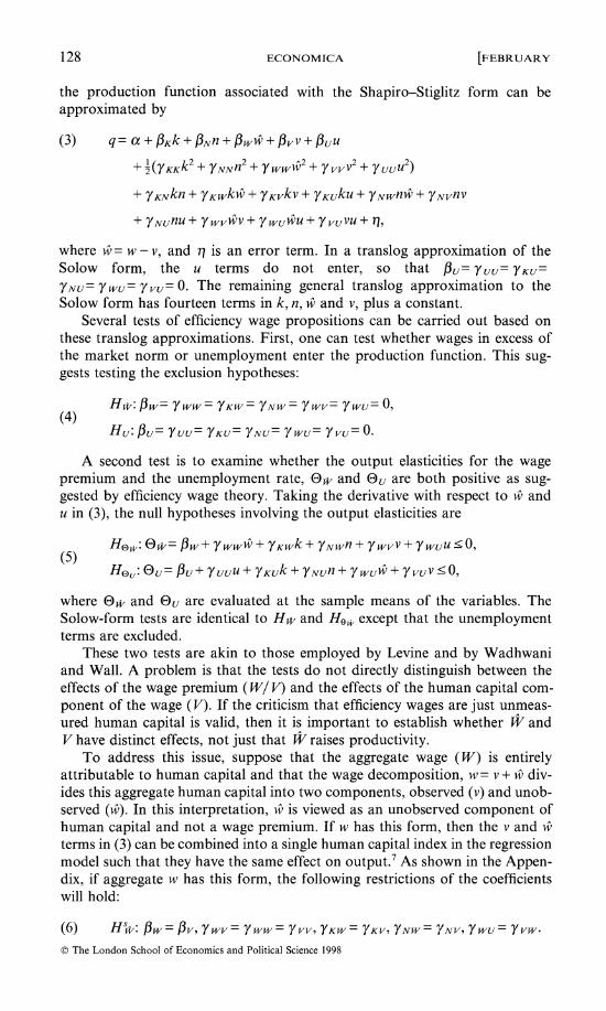
the production function associated with the Shapiro-Stiglitz form can be approximated by

(3) q= a + PKk +PNn + PWw + PVv + Puu

+ 1(yKKk2 + YNNn 2 + 7WWV + yVVV2 + yUUU2)

+ yKNkn + YKWkW + YKVkV + YKUkU + YNwnfW + YNvnv

+ YNU nu +WV wvWV + YwWUiWU + YvuVU + 11,

where wv = w - v, and i7 is an error term. In a translog approximation of the Solow form, the u terms do not enter, so that Bu= 'Yuu= YKU=

YNU=7WU=7vu=0. The remaining general translog approximation to the Solow form has fourteen terms in k, n, vw and v, plus a constant.

Several tests of efficiency wage propositions can be carried out based on these translog approximations. First, one can test whether wages in excess of the market norm or unemployment enter the production function. This sug- gests testing the exclusion hypotheses:

H,: pw= Yww= YKW= YNW= YWV= YWU= 0, (4)

Hu: PU= Yuu= YKU= YNU= YWU= YVU= 0-

A second test is to examine whether the output elasticities for the wage premium and the unemployment rate, Oa and Ou are both positive as sug- gested by efficiency wage theory. Taking the derivative with respect to Vw and u in (3), the null hypotheses involving the output elasticities are

( He3w :)wf,Bw+ ywwVY +yKwk +yNwn + ywvV + ywuU ? O,

HOU: OU= U3+ YUUU + YKUk+ YNUn+ }ywuW + YuV?! O,

where Oa, and Ou are evaluated at the sample means of the variables. The Solow-form tests are identical to HW and How, except that the unemployment terms are excluded.

These two tests are akin to those employed by Levine and by Wadhwani and Wall. A problem is that the tests do not directly distinguish between the effects of the wage premium (WI V) and the effects of the human capital component of the wage (V). If the criticism that efficiency wages are just unmeasured human capital is valid, then it is important to establish whether W and V have distinct effects, not just that W raises productivity.

To address this issue, suppose that the aggregate wage (W) is entirely attributable to human capital and that the wage decomposition, w = v + Vw div- ides this aggregate human capital into two components, observed (v) and unobserved (vw). In this interpretation, vw is viewed as an unobserved component of human capital and not a wage premium. If w has this form, then the v and Vw terms in (3) can be combined into a single human capital index in the regression model such that they have the same effect on output.7 As shown in the Appen- dix, if aggregate w has this form, the following restrictions of the coefficients will hold:

(6) Hw: fw= fv, Ywv= Yww= YVV, YKW= 1(KV, YNW= YNV, YWU= YVW-

? The London School of Economics and Political Science 1998


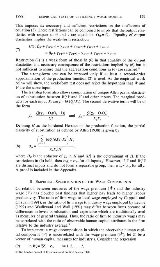
This imposes six necessary and sufficient restrictions on the coefficients of equation (3). These restrictions can be combined to imply that the output elasticities with respect to vw and v are equal, i.e. O,= Ov. Equality of output elasticities implies the weak-form restriction

HW': fw+ yvWWI + yKwk + YNWn + YwvV + YwuU

= 3V + YVVV + YKvk+ YNvvn + 7 wvW + Y vuu.

Restriction (7) is a weak form of those in (6) in that equality of the output elasticities is a necessary consequence of the restrictions implied by (6) but is not sufficient to insure that the aggregation conditions in (6) are satisfied.8

The strong-form test can be imposed only if at least a second-order approximation of the production function (2) is used. As the empirical work below will show, the weak-form test does not reject the hypothesis that W and V are the same input.

The translog form also allows computation of unique Allen partial elasticities of substitution between W/ V and V and other inputs. The marginal products for each input Xi are fi= Oi(Q/Xi). The second derivative terms will be of the form

Q(y+ii O(Oi -1)) and fij= Q(7ij+e)iOj) i Xi Xi

Defining H as the bordered Hessian of the production function, the partial elasticity of substitution as defined by Allen (1938) is given by

( ( (aQ/lXk) Xk) Hi \k= 1/

(8) (Tij = -jH XiXIIHI

where Hij is the cofactor offij in H and IHI is the determinant of H. If the restrictions in (6) hold, then a wj= a vj for all inputs j. However, if V and WI V are distinct inputs and do not form a separable group, then a wj a vj for allj. A proof is included in the Appendix.

II. EMPIRICAL SPECIFICATION OF THE WAGE COMPONENTS

Correlation between measures of the wage premium (W) and the industry wage (V) has clouded past findings that higher pay leads to higher labour productivity. The ratio of firm wage to local wage employed by Cappelli and Chauvin (1991), or the ratio of firm wage to industry wage employed by Levine (1992) and Wadhwani and Wall (1991) may differ between firms because of differences in levels of education and experience which are traditionally used as measures of general training. Thus, the ratio of firm to industry wages may be correlated with the ratio of observable human capital attributes in the firm relative to the industry average.9

To implement a wage decomposition in which the observable human capital component (V) is uncorrelated with the wage premium (W), let Zi be a vector of human capital measures for industry i. Consider the regression

(9) ln Wi = EZi + ai, iP= 1i 2a .S. cI I, C) The London School of Economics and Political Science 1998


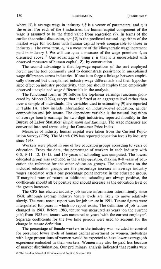
where Wi is average wage in industry i, 4 is a vector of parameters, and Ei is the error. For each of the I industries, the human capital component of the wage is assumed to be the fitted value from regression (9). In terms of the earlier theoretical discussion, vi= 4Zi is the predicted natural logarithm of the market wage for workers with human capital levels comparable to those in industry i. The error term, Ei, is a measure of the idiosyncratic wage increment paid in industry i. We will use Ei as a measure of the wage premium vi as discussed above.10 One advantage of using Ei is that it is uncorrelated with observed measures of human capital, Zi, by construction.

The second advantage is that log-wage equations of the sort employed herein are the tool commonly used to demonstrate persistence in unexplained wage differences across industries. If one is to forge a linkage between empirically observed but unexplained industry wage differentials and their hypothe- sized effect on industry productivity, then one should employ these empirically observed unexplained wage differentials in the analysis.

The functional form in (9) follows the log-linear earnings functions pion- eered by Mincer (1974), except that it is fitted at an aggregate level rather than over a sample of individuals. The variables used in estimating (9) are reported in Table IA. They include information on industry-level education, gender composition and job tenure. The dependent variable is the natural logarithm of average hourly earnings for two-digit industries, reported monthly in the Bureau of Labor Statistics' Employment and Earnings. The wage measures are converted into real terms using the Consumer Price Index.

Measures of industry human capital were taken from the Current Popu- lation Survey (CPS). The March CPS has reported education levels by industry since 1968.

Workers were placed in one of five education groups according to years of education. From the data, the percentage of workers in each industry with 0-8, 9-11, 12, 13-15, and 16+ years of schooling was computed. The lowest educated group was excluded in the wage equation, making 0-8 years of education the reference for the other education groups. The coefficients on the included education groups are the percentage increase in average industry wages associated with a one percentage point increase in the educated group. If marginal rates of return to additional schooling are always positive, the coefficients should all be positive and should increase as the education level of the group increases.

The CPS has elicited industry job tenure information intermittently since 1968, although average industry tenure levels are likely to move relatively slowly. The most recent report was for job tenure in 1991. Tenure figures were interpolated for years in which no report exists. The definition of job tenure changed in 1983. Before 1983, tenure was measured as years 'on the current job'; from 1983 on, tenure was measured as years 'with the current employer'. Separate coefficients for the two time periods were used to account for the change in tenure definition.

The percentage of female workers in the industry was included to control for presumed lower levels of human capital investment by women. Industries with large proportions of women would be expected to have lower average job experience embodied in their workers. Women may also be paid less because of market discrimination. Our preliminary analysis indicated that results were ? The London School of Economics and Political Science 1998


TABLE 1

VARIABLE DEFINITIONS AND SAMPLE STATISTICSa

Standard Mean deviation

A: Wage function Dependent variable Al Natural logarithm of average hourly wage (EE) deflated

by the Consumer Price Index 2 15 0 22 Independent variables A2 Average years of education (CPS) 12-30 0.59 A3 Average job tenure 1968-82 (CPS)

and zero otherwise 3 18 2 91 A4 Average job tenure 1983-91 (CPS)

and zero otherwise 2 46 3 41 A5 Per cent female (CPS) 31 00 17 8 A6 Per cent with at most 8 years of education 14 40 9.1 A7 Per cent with 9-11 years of education 17 10 5 8 A8 Per cent with 12 years of education 43 40 5 4 A9 Per cent with 13-15 years of education 13-20 4 9 AIO Per cent with 16+years of education 11 90 7.4

B. Production function Dependent variable Bi Natural logarithm of weighted industrial production

(FR) 5 62 0 78 Independent variables (in natural logarithms) B2 Number of workers in the industry (EE) 6 76 0 69 B3 Number of workers in the industry (CPS) 6 80 0 68 B4 Average hours per week (EE) times B2 10 54 0 63 B5 Average hours per week (EE) times B3 10 58 0 64 B6 Constant cost net stock of fixed private capital (SCB) 3 45 0.99 B7 Unemployment rate in durable and nondurable goods

industries (MLR) 1 84 0 33 B8 Human capital component of the wage (fitted value

from eqn (9) 2 15 021 B9 Wage increment

(error term in eqn (9)) 0 00 0 076

a The unit of observation is the two-digit manufacturing industries excluding textiles and miscellaneous manufacturing over the 1968-88 sample period. Sources: EE = Employment and Earnings; CPS = Current Population Survey; FR = Federal Reserve Board of Governors; SCB = Survey of Current Business; MLR = Monthly Labor Review. All variables are March monthly figures except as discussed in the text.

similar whether or not per cent female was included among the human capital measures.

The specification of the earnings function concentrates on human capital variables only. The intent is to estimate the wage premium as the portion of the wage uncorrelated with observable human capital. For this reason, controls for union status were deliberately excluded. Unions may target sectors in which efficiency wages are most important (and wages least sensitive to cyclical pres- sures). Thus, removing estimated union effects might also remove efficiency wage effects."1 Similarly, industry dummy variables were not included since the dummy variables would also remove potential efficiency wage effects. Indeed, ? The London School of Economics and Political Science 1998


industry dummy variable coefficients were used by Krueger and Summers and by Katz and Summers as their estimates of industry efficiency wages.

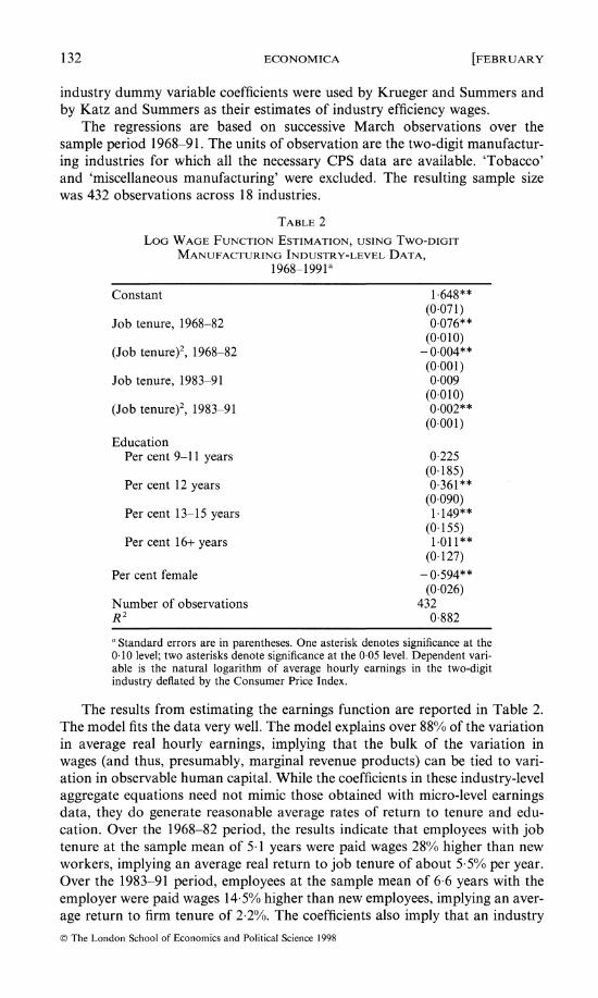
The regressions are based on successive March observations over the sample period 1968-91. The units of observation are the two-digit manufacturing industries for which all the necessary CPS data are available. 'Tobacco' and 'miscellaneous manufacturing' were excluded. The resulting sample size was 432 observations across 18 industries.

TABLE 2

LOG WAGE FUNCTION ESTIMATION, USING TWO-DIGIT

MANUFACTURING INDUSTRY-LEVEL DATA,

1968-1 991a

Constant 1648** (0.071)

Job tenure, 1968-82 0.076** (0.010)

(Job tenure)2, 1968-82 - 0.004** (0 001)

Job tenure, 1983-91 0-009 (0 010)

(Job tenure)2, 1983-91 0.002** (0.001)

Education Per cent 9-11 years 0 225

(0.185) Per cent 12 years 0 361**

(0.090) Per cent 13-15 years 1.149**

(0.155) Per cent 16+ years 1011'**

(0 127)

Per cent female - 0594** (0 026)

Number of observations 432 R 2 00882

a Standard errors are in parentheses. One asterisk denotes significance at the 0 10 level; two asterisks denote significance at the 0 05 level. Dependent variable is the natural logarithm of average hourly earnings in the two-digit industry deflated by the Consumer Price Index.

The results from estimating the earnings function are reported in Table 2. The model fits the data very well. The model explains over 88% of the variation in average real hourly earnings, implying that the bulk of the variation in wages (and thus, presumably, marginal revenue products) can be tied to variation in observable human capital. While the coefficients in these industry-level aggregate equations need not mimic those obtained with micro-level earnings data, they do generate reasonable average rates of return to tenure and education. Over the 1968-82 period, the results indicate that employees with job tenure at the sample mean of 5 1 years were paid wages 28% higher than new workers, implying an average real return to job tenure of about 5.5% per year. Over the 1983-91 period, employees at the sample mean of 6.6 years with the employer were paid wages 14.5% higher than new employees, implying an average return to firm tenure of 2.2%. The coefficients also imply that an industry ? The London School of Economics and Political Science 1998


employing only high school graduates (those with 12 years of schooling) would pay wages 36% higher than wages in an industry employing only workers with eight years of schooling. The implied real rate of return to 12 years of schooling relative to eight years is 9% per year. Similar computations imply a real rate of return to a college degree relative to eight years of schooling of 12.5% per year. The wage equation also shows that predominantly female industries pay lower wages than predominantly male industries, with a 10 percentage point increase in female employees resulting in a 6% reduction in real wages. These estimated rates of return are comparable with those obtained using micro-level data. 12

The measured industry wage premium, Ei, will be uncorrelated with observed levels of education, proportion female and job tenure in the industry. Even though these observed human capital measures fail to explain only 12% of the variation in wages across industries and time, it is conceivable that additional measures of human capital would explain some or all of the remaining variation in Ei. Thus, we cannot assert that Ei is an efficiency wage, unobserved human capital, or anything else. This identification problem will occur regardless of how well the Zi in (9) are specified, since the residuals are, by definition, what is not known about the wage. Nevertheless, differences in how the estimated ci and vi enter the estimated production process can establish if the ?i are consistent with efficiency wages.

III. PRODUCTION FUNCTION ESTIMATION

The predicted and unexplained components of log wage enter as inputs into the production function. Other inputs are labour and the capital stock. Two measures of the number of workers in the industry in March are available: the Current Population Survey and Employment and Earnings. Employment and Earnings also reports average hours worked per week for a subset of the industries, so a measure of total hours (number of workers times average hours per week) as an alternate measure of employment is also used.13 Results are reported for four measures of labour input, defined as B2-B5 in Table 1. The capital stock measure is the 'constant cost net stock of fixed private capital', which is published in the Survey of Current Business. This is an annual measure, but it is assumed that the aggregate industry capital stock grows slowly enough to allow the annual measure to proxy the capital stock in place in March.

The output measure is the Federal Reserve's two-digit Industry Index of Industrial Production. These indices are reported in constant 1982 dollars. To obtain relative output size across industries, the industry output indices were multiplied by their respective industry weights as reported by the Federal Reserve. The sample statistics for the output and input measures are reported in Table lB.

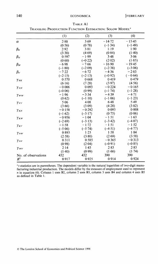
Estimation of the Solow model

Production function estimates for the Solow model, which ignores unemployment effects, are reported in Appendix Table Al. The model fitted the data quite well, with over 90% of the variance in industry output explained by the inputs. More important are tests of the hypotheses described by (4) and (5). ? The London School of Economics and Political Science 1998


Because the production function uses generated regressors, OLS standard errors are not efficient. All tests use White's (1980) correction for heteroscedasticity. In addition, a second set of tests based on a bootstrapping procedure yielded nearly identical results. Conclusions were not overly sensitive to the use of OLS, White or bootstrap-generated standard errors.

The exclusion tests for each input in the Solow form of the translog production function are reported in Table 3(a). The null hypothesis that a variable

TABLE 3

COMPUTED EXCLUSION TEST STATISTICS AND OUTPUT ELASTICITIES BASED ON THE TRANSLOG FORM OF THE SOLOW MODEL

Variablea (1)b (2) (3) (4)

(a) Exclusion tests K 831.9** 825.2** 759.3** 730.0** N 1911 .0** 1840.7** 1515.9** 1479. 1 ** W 9.3** 14.5 ** 17.9** 20.9** V 79.0** 92.2** 85.0** 94.2** F0.05c 2 24 2 24 2 24 2 24

(b) Output elasticities de

K 0.42** 0.44** 0.38** 0.37** (0 01) (0.01) (0.01) (0.01)

N 0.68** 0.68** 0.64** 0.67** (0 01) (0.01) (0.01) (0.01)

W 0.35** 0. 19** 0.61** 0.47** (0 09) (0 09) (0.10) (0.10)

V 0.30** 0.10* 0.51** 0.41** (0.06) (0 06) (0 06) (0 06)

a Variable notation corresponds to that in the text. One asterisk denotes significance at the 010 level; two asterisks denote significance at the 0 05 level. b Equations differ by the empirical measure of employment utilized. Column (1) uses definition B2 for N, column (2) uses B3, column (3) uses B4 and column (4) uses B5, as defined in Table 1. 'Approximate critical value of the corrected F-statistic. dComputed at sample means for the variable except when noted. eCorrected standard errors in parentheses.

can be excluded is strongly rejected in every case. These conclusions are not sensitive to changes in the definition of employment.

The estimated output elasticities and their associated significance levels are reported in Table 3(b). All output elasticities are below one, as required by theory, and all are positive. The wage premium has output elasticities that are positive and significant in all four cases. The magnitudes of the elasticities vary between 0 19 and 0 61, bracketing those reported by Levine (0.46) and Wadhwani and Wall (0.39). The output elasticity for employment varies from 0 64 to 0 68 compared with Wadhwani and Wall's estimate of 0 65. The con- clusion from tests of hypothesis (5) is that wage premia do appear to have productive effects at the industry level that are similar in magnitude to those reported at the firm level.

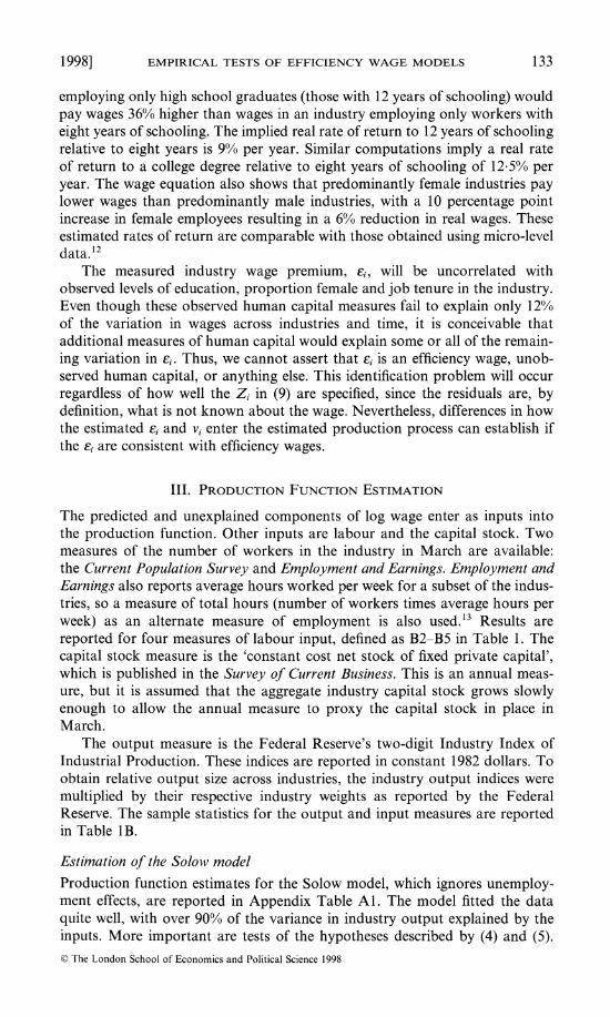
While the output elasticities for W are consistent with the efficiency wage proposition, they are not very different from the output elasticities computed for the observed human capital component of the wage (W). As reported in Table 4, the weak-form (necessary condition) test (7) that O,= Ov could not ? The London School of Economics and Political Science 1998


TABLE 4 WEAK- AND STRONG-FORM TESTS OF THE HYPOTHESIS THAT THE

HUMAN CAPITAL (V) AND WAGE PREMIUM (J) COMPONENTS CAN BE AGGREGATEDa

Solow Shapiro-Stiglitz

1 2 3 4 1 2 3 4

(a) Weak-form test using equation (7) 024 082 078 023 004 0 15 053 0 18

F0.05 3 86 3 86 3 86 3 86 3 86 3286 3 86 3 86

(b) Strong-form test using equation (6) 15.0** 17 1** 27.2** 27.9** 14.2** 15.3** 22.9** 23.4**

F0.05 224 224 224 224 2 12 2 12 2 12 2 12

'All tests based on the White (1980) correction for heteroscedasticity. One asterisk denotes significance at the 0 10 level; two asterisks denote significance at the 0 05 level.

be rejected at standard significance levels. Because observable human capital explains 88% of the variation in average wages across industries, the equal output elasticities with respect to the two wage components imply that observable human capital is also responsible for 88% of the effect of average industry wages on output. Only 12% of the wage effect on output is associated with the wage premia. However, the strong-form (necessary and sufficient condition) test (6), which imposes equality on the second-derivative terms for v and wi, strongly rejected the null hypothesis that the observed and unobserved components of the industry wage could be aggregated into a single input. Thus, the effects of W and V are distinct, and Allen elasticities of substitution between these and other inputs are not equal.

Shapiro-Stiglitz model estimation

The same battery of tests was applied to the translog form of the Shapiro- Stiglitz shirking model. The input set includes the variables in the Solow model plus the March unemployment rate as reported in the Monthly Labor Review. We used the overall durable (nondurable) unemployment rate to reflect the probability of unemployment for specific two-digit durable (nondurable) industries. 14

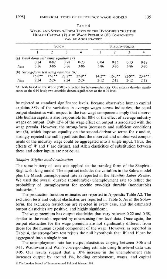
The production function estimates are reported in Appendix Table A2. The exclusion tests and output elasticities are reported in Table 5. As in the Solow form, the exclusion restrictions are rejected in every case, and the estimated output elasticities are positive, and highly significant.

The wage premium has output elasticities that vary between 0 22 and 0 58, similar to the results reported by others using firm-level data. Once again, the output elasticities for the wage premium are not significantly different from those for the human capital component of the wage. However, as reported in Table 4, the strong-form test rejects the null hypothesis that W and V can be aggregated into a single input.

The unemployment rate has output elasticities varying between 0 06 and 0. 11; Wadhwani and Wall's corresponding estimate using firm-level data was 0 05. Our results suggest that a 10% increase in the unemployment rate increases output by around 1%, holding employment, wages, and capital ? The London School of Economics and Political Science 1998


TABLE 5

COMPUTED EXCLUSION TEST STATISTICS AND OUTPUT ELASTICITIES BASED ON THE TRANSLOG FORM OF THE SHAPIRO-STIGLITZ MODEL

Variablea (1 )b (2) (3) (4)

(a) Exclusion tests K 642. 1** 619.7** 602.7** 569.2** N 1531.8** 1509.5** 1228.9** 1224.7** W 13. 1** 15.8** 20. 1** 21.7** V 74.4** 78.9** 75.0** 80.0** U 65.5** 58.7** 66.4** 58.9** FO005C 2 12 2 12 2 12 2 12

(b) Output elasticitiesd K 0.39** 0.41** 0.35** 0.34**

(0 01) (0 01) (0 01) (0.01) N 0.71** 0.70** 0.69** 0.71**

(0.01) (0 01) (0 01) (0.01) W'V 0.33** 0.22** 0.58** 0.48**

(0 09) (0.09) (0.10) (0 10) V 0.36** 0. 18** 0.49** 0.43**

(0 06) (0 06) (0.06) (0.06) U 0.07** 0.06** 0.11** 0.09*

(0 01) (0.01) (0.01) (0.01)

Note: See Table 3 for footnotes and other details.

fixed.15 The positive output elasticities for both wage premia and the unemployment rate imply the existence of a negative trade-off between unemployment rates and wages, consistent with the 'wage curve' findings of Blanchflower and Oswald (1994).

These Solow and Shapiro-Stiglitz estimates may be subject to the criticism that wages, wage premia and output are jointly determined. As such, our estimates may be clouded by simultaneity bias. Hausman tests, which used lagged input values, wages, prices and unemployment rates as instruments, were applied to the Cobb-Douglas forms of the Solow and Shapiro-Stiglitz production relationships. In all eight cases, the Hausman tests failed to reject the null hypothesis of exogeneity at the 5% level.

Elasticities of substitution

As pointed out previously and in the Appendix, if W and V are distinct inputs, then Allen partial elasticities of substitution between these inputs and others will be distinct. Using the coefficients reported in the Appendix, eight matrices of Allen partials were estimated. However, in the Shapiro-Stiglitz form, the adjoint of the bordered Hessians failed to produce positive elements along the diagonal in all four instances. Thus, the production function was not locally concave when evaluated at sample means.16 Concavity is necessary to ensure that the own partials are negative as required by economic theory.

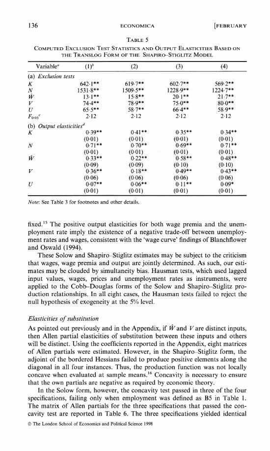
In the Solow form, however, the concavity test passed in three of the four specifications, failing only when employment was defined as B5 in Table 1. The matrix of Allen partials for the three specifications that passed the concavity test are reported in Table 6. The three specifications yielded identical ? The London School of Economics and Political Science 1998


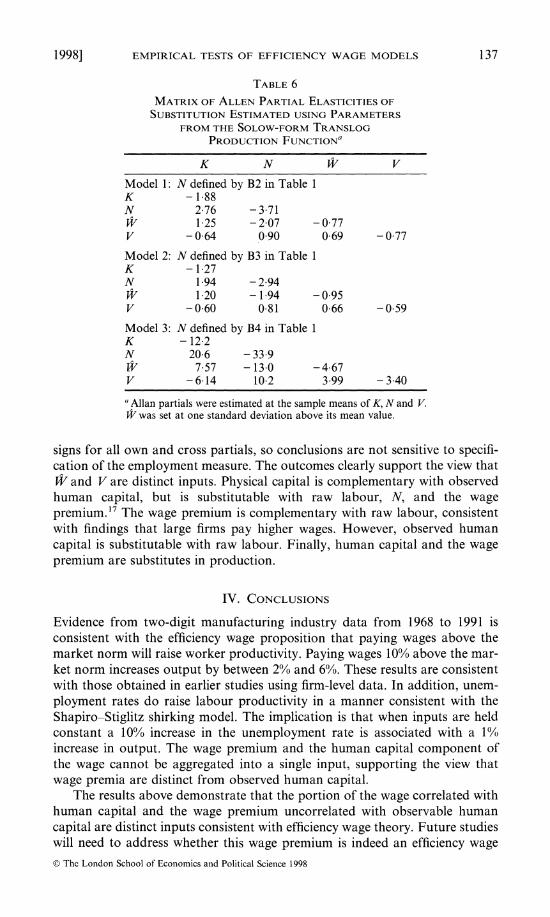
TABLE 6

MATRIX OF ALLEN PARTIAL ELASTICITIES OF

SUBSTITUTION ESTIMATED USING PARAMETERS

FROM THE SOLOW-FORM TRANSLOG

PRODUCTION FUNCTIONa

K N W V

Model 1: N defined by B2 in Table 1 K -1 88 N 276 -371 W 1 25 -207 -0777 V -064 090 069 -077

Model 2: N defined by B3 in Table 1 K -1 27 N 1 94 - 2 94 W 1.20 -1 94 -095 V -060 081 066 -059

Model 3: N defined by B4 in Table 1 K -12.2 N 206 -339 W 7.57 - 130 -4667 V -614 102 399 -340

a Allan partials were estimated at the sample means of K, N and V. W was set at one standard deviation above its mean value.

signs for all own and cross partials, so conclusions are not sensitive to specification of the employment measure. The outcomes clearly support the view that W and V are distinct inputs. Physical capital is complementary with observed human capital, but is substitutable with raw labour, N, and the wage premium.17 The wage premium is complementary with raw labour, consistent with findings that large firms pay higher wages. However, observed human capital is substitutable with raw labour. Finally, human capital and the wage premium are substitutes in production.

IV. CONCLUSIONS

Evidence from two-digit manufacturing industry data from 1968 to 1991 is consistent with the efficiency wage proposition that paying wages above the market norm will raise worker productivity. Paying wages 10% above the market norm increases output by between 2% and 6%. These results are consistent with those obtained in earlier studies using firm-level data. In addition, unemployment rates do raise labour productivity in a manner consistent with the Shapiro-Stiglitz shirking model. The implication is that when inputs are held constant a 10% increase in the unemployment rate is associated with a 1% increase in output. The wage premium and the human capital component of the wage cannot be aggregated into a single input, supporting the view that wage premia are distinct from observed human capital.

The results above demonstrate that the portion of the wage correlated with human capital and the wage premium uncorrelated with observable human capital are distinct inputs consistent with efficiency wage theory. Future studies will need to address whether this wage premium is indeed an efficiency wage ? The London School of Economics and Political Science 1998


or some type of human capital not explained by typically used factors such as education, job experience or tenure. Nevertheless, this wage premium represents only 12% of the variation in wages across industries. The remaining 88% of the wage is explainable by measures of general human capital. Thus, the majority of the productivity effect associated with differing relative wages across industries can be tied to variation in observable human capital.

ACKNOWLEDGMENTS

The authors acknowledge the helpful comments of the referees and also those of Barry Falk, Wallace Huffman, Peter Mattila, John Schroeter, Howard Van Auken and seminar participants at Iowa State University. Donna Otto prepared the manuscript.

APPENDIX

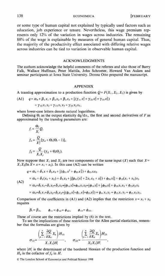
A translog approximation to a production function Q= F(XI, X2, X3) is given by

(Al) q= aoo+px1+1X2x2+X3x3+X(y11x21+y22x2+y33x3)

+ YI2XI X2 + '13X1 X3 + 723X2X3,

where lower-case letters denote natural logarithms. Defining E0i as the output elasticity dq/dxi, the first and second derivatives of F as

approximated by the translog parameters are:

Exi fi Q

fii = Q [yii + Oi(E)i - 1 )], xi

fii= Xi (yu + OiOj).

Now suppose that X1 and X2 are two components of the same input (X) such that X= X1 X2(ln X= x= xi + x2). In this case (A2) can be written

q= aO + 51 X + 63X3 + 2(p11X2 + 0p33X3)+ 0p13XX3

= O 5 1 (XI + X2) + 653X3 + 2[1 (12 + 2X1X2 + 2) 033 X32 + 013 (X1I+ X2)X3 (A2) 2o 2+ X

= ao+3X1X1+31X2+63X3 11+(11x1I-X-X2+2p11X2 + 12033X3 + 013X1X3 + 013X2X3

= ao+31X1+31X2+53X3+2-((I 11+01 xIX2+033X3) + 11XI X2 + 013X1 X3 + 013X2X3.

Comparison of the coefficients in (Al) and (A2) implies that the restriction x= xI + x2 requires

P = 32, 011 = P12= 022, (13= 023.

These of course are the restrictions implied by (6) in the text. To see the implications of these restrictions for the Allen partial elasticities, remem-

ber that the formulas are given by

n aQ Xk H13

n a Q Xk H23

k= I aXk _kk=1 I Xk/

X, X3 IHI X2x3 IHI where IHI is the determinant of the bordered Hessian of the production function and Hqi is the cofactor off; in H.



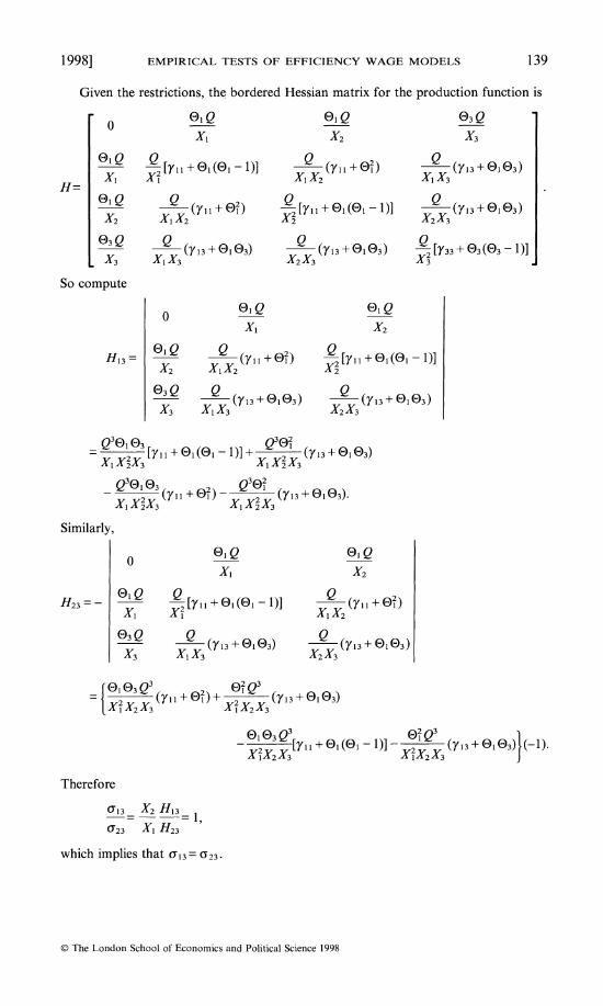
Given the restrictions, the bordered Hessian matrix for the production function is

0 OiE Q E)i Q 03 Q

X1 X2 X3

E__ Q Q I )) Q Oi

| X, x2[1+E,(E,-1 1)] ((71+3 (13+01 03)

H= Xi xI XIx2 XI x3

Ei,Q Q (yll+E)2) Q Q x1x ~ I

,2 [7yi11+0E1(E01- 1)] (7 13 +01 03) X2 XI X2 212 X2 X3

03Q XQ (Y13+ ,01 03) - (y 13+0103) x2[Y33+E)3(E)3 -

01 x3 XIx3 x2 x33 So compute

O OiQ E3iQ

X1 X2

H13= OQ Q Q H13 = 2 XX(y1 I 012 -2 [y, 1 + E), (E), - 1)]

1 2 XI 1 A 2

03 Q (7 13 +01 03) ( 7 ( 13 ++01 03)

X3 XI3 X 2 X 3

Q3E)0 E__ 3E_

Similarly,

O (3'OQ Oi)Q x1 x2

03Q XQ (713+01033) X (713+010()

= t

' (711 + Ol)+X2XXQ(713 + O13) X, X2X3 X, 03_

y EE - ] (1[73 +01 (01 -1)] 0xQ3 (713+0103)j(-1).

Therefore

0X3= X2 13 023 X, (23

which implies that 3 = (s23.



TABLE Al

TRANSLOG PRODUCTION FUNCTION ESTIMATION: SOLOW MODEL"

(1) (2) (3) (4)

a 288 369 -1472 -1545 (0.56) (0.78) (-1.34) (-1 49)

[K 2 92 3 81 1.19 1.90 (3 38) (469) (084) (1.40)

ON 0-597 -199 3 48 3 06 (060) (-022) (202) (1 85)

13w -698 -766 -1690 -1945 (-1.80) (-209) (-238) (-306)

13V -722 -672 -436 -283 (-2.15) (-2 13) (-092) (-0.64)

YKK 0 570 0 668 0 419 0 479 (6.16) (7 28) (3 97) (4 56)

YNN -0006 0 093 -0 224 -0 165 (-006) (099) (-1 74) (-1.28)

Yww - 1 96 -3 34 -4 39 -4 71 (0 62) (-1.10) (-1 06) (-1.23)

Yvv 5 06 4 08 6 48 5s49 (3 66) (3 09) (4 28) (3.82)

YKN -0158 -0292 0 093 0 008 (-1.62) (-3 17) (0 75) (0.06)

YKW -0956 - 1 04 -1.51 - 1 63 (-2.69) (-3 13) (-3.42) (-4.07)

YKV -158 - 1 72 - 1.51 - 1 52 (-5.06) (-5.74) (-4 51) (-4*77)

YNW 0 893 1 23 1 58 1 84 (2.58) (380) (2.69) (3.58)

YNV 0 311 0 585 -0 365 -0 313 (0 98) (2 04) (-0.91) (-0.85)

YWV 2 14 1 43 2 83 2 83 (1.40) (0.99) (1.66) (1.74)

No. of observations 432 432 390 390 RJ2 0 917 0 925 0 914 0 924

a t-statistics are in parentheses. The dependent variable is the natural logarithm of two-digit manufacturing industrial production. The models differ by the measure of employment used to represent n in equation (6). Column I uses B2, column 2 uses B3, column 3 uses B4 and column 4 uses B5 as defined in Table 1.



TABLE A2

TRANSLOG PRODUCTION FUNCTION ESTIMATION: SHAPIRO-STIGLITZ MODELa

(1) (2) (3) (4)

a - 0 497 - 0 269 - 14-24 - 17 58 (-009) (-0.05) (-1 17) (-1 59)

[K 3 39 3 97 2 54 2 66 (3.76) (4.74) (1.67) (1.88)

ON 0 342 -0 197 2 28 2 43 (0 33) (-0.21) (1.23) (1.42)

13w - 8 91 - 7 58 - 20 99 - 20 52 (-2.09) (-1.92) (-2.85) (-3.15)

13V - 5 37 - 4 87 - 2 24 - 0 401 (-1.56) (1.52) (-0.46) (-0.09)

1u 1 40 1 70 1 07 1 45 (1.66) (2.18) (0.88) (1.34)

YKK 0 635 0 697 0 538 0 553 (6.78) (7 59) (4.90) (5.17)

YNN 0.041 0 103 -0 109 -0 097 (042) (1.12) (-081) (-075)

Yww -0181 -160 -369 -365 (-0 06) (-0 52) (-0 89) (-0 95)

7VV 417 3.49 4.74 423 (3 06) (2 68) (3.11) (2 95)

Yuu -0 579 -0 611 -0 516 -0 540 (-4 23) (-4 71) (-3 50) (-3 93)

7KN -0228 -0320 -0 058 -0 083 (-2 33) (-3 51) (-0 44) (-0 68)

7KW -1.11 - 1 10 - 1 70 - 1 73 (-3.07) (-3 25) (-3 84) (-4 31)

7KV -163 - 1 74 - 1 52 - 1 52 (-5 27) (-5 88) (-4.60) (-4 83)

7KU -0 082 -0 030 -0 095 -0 045 (-1 10) (-043) (-1.16) (-061)

YNW 1 07 1 25 1 96 1 99 (3 01) (3 78) (3.34) (3 89)

7NV 0-380 0-590 -0-172 -0.230 (1.19) (2 08) (-0.41) (-0 62)

7NU 0-035 0 020 0 073 0 044 (0 49) (0 30) (0 75) (0 51)

7wv 1 92 0.991 2 52 2 39 (1.26) (0 69) (1.47) (1.47)

7Wu 0 931 0 535 0 717 0 448 (1 86) (1.14) (1.28) (0 86)

7vu -0 096 -0 252 -0 208 -0 310 (-0.33) (-0.91) (-0 66) (1 06)

No. of observations 432 432 390 390 R 2 00924 0 931 0 921 0 930

See Table Al for footnotes and other details.



NOTES

1. Kniesner and Goldsmith (1987) reported that the elasticity of nominal wages to aggregate output over the 1948-85 period was 0 004.

2. Reviews of the literature include Akerlof and Yellen (1986); Katz (1986); and Stiglitz (1987). 3. Perhaps the best example of this is the study by Cappelli and Chauvin (1991), who found that

increasing wages relative to local wages significantly decreased the rate of disciplinary layoffs in a single multi-plant firm. On the other hand, the average aninual rate of disciplinary layoffs across plants in their sample was 10%. Unexplained is why, if indeed this firm was paying efficiency wages, its overall disciplinary layoff rate was so high.

4. Both Levine and Wadhwani and Wall tried production function specifications that included some second-order terms, but neither used a fully specified flexible form. Levine (1992, p. 1110) stated that the Cobb-Douglas form was misspecified and led to heteroscedastic errors. Our own data-set also strongly rejects the Cobb-Douglas form in favour of the flexible form.

5. Layard et al. (1991, p. 164 and Annex 3.1) and Wadhwani and Wall (1991, pp. 531-3) provide useful discussions of this point.

6. Inclusion of both W and V in the production function requires that the overall wage (W= WV) be decomposed into the portion of the wage that is due to human capital (V) and the portion unexplained by human capital (W). Inclusion of both terms allows separate productivity effects for workers' skills and wage premiums.

7. These tests are similar in spirit to Berndt and Christensen's (1974) tests of whether labour types can be aggregated into a single labour index.

8. This distinction is critical because the weak form test (7) is consistent with the Cobb-Douglas specifications imposed in earlier studies.

9. Even direct use of industry averages of residuals from log-earnings functions based on individual-level data may be insufficient to purge wage premia of observable human capital effects. Schultze (1989) and Murphy and Topel (1990) argued that 'unexplained' industry wage differentials of the type reported by Krueger and Summers (1988) and by Katz and Summers (1989) were still correlated with average levels of human capital characteristics in those industries. This result is consistent with a sorting model in which high-productivity workers sort into high-wage sectors and low-productivity workers sort into low-wage sectors.

10. The wage paid in industry i relative to the market opportunities of its workers is Wi/ Vi. This can be rewritten as 1 + Xi, where A, = (Wi - Vi)! Vi is the proportional wage increment over the market norm paid in industry i. If Xi is small, ln (Wi/ Vi) = Ei A Xi and ln Vi = gZi.

11. An auxiliary regression of our estimated wage premium on 'per cent union' found that union density explains 14% of the variation in our estimated wage premium, so the wage premium is not dominated by union effects.

12. Topel (1991) reported an annual return of 4 1/% at five years of job tenure and 3.3% at seven years of job tenure. Willis (1986) reported that returns to high school varied from 10% to 12% while returns to college varied from 8% to 10%. His estimates cover only the first half of our sample. Starting in 1979, Juhn et al. (1993) reported a dramatic increase in returns to college relative to high school. Therefore, over the 1968-91 period, it is plausible that average returns to college have exceeded average returns to high school.

13. Two industries (petroleum, and rubber and plastics) did not have data on average hours, and so fall out of the production function estimation when labour is measured by total hours rather than number of employees.

14. The issue of which unemployment rate to use is a bit speculative. In a sense, an unemployed worker is equally unemployed in every sector, but the worker will seek employment only in the subset of markets for which expected return from search will exceed expected costs. Our use of durable and nondurable goods unemployment rates implicitly assumes that displaced manufacturing workers will continue to seek employment in manufacturing, although perhaps not in the same two-digit industry.

15. The output elasticity for employment is ten times larger than that for the unemployment rate. The literal interpretation is that if, in a cyclical downturn, the unemployment rate rises more than ten times faster than employment falls, total output could actually rise, since the productive impact of the increase in the unemployment rate would outweigh the lost output resulting from smaller employment. An examination of typical employment and unemployment rates over business cycles between 1968 and 1991 found that the increased productivity from increased unemployment was of roughly equal magnitude to the decreased productivity from lost employment.

16. Estimates were at sample means for all variables except w~, which was set at one standard deviation above the mean. The mean of w~ is 0 by construction.

17. These results are consistent with the Griliches (1969) hypothesis that skilled labour is complementary with capital whereas unskilled labour and capital are substitutes. In all three cases where the concavity requirement was satisfied, a VK 0< ?aNK.



REFERENCES

AKERLOF, G. A. and YELLEN, J. L. (1986). Efficiency Wage Models of the Labour Market. Cam- bridge University Press. 1986.

ALLEN, R. G. D. (1938). Mathematical Analysis for Economists. London: Macmillan. BECKER, G. (1964). Human Capital. New York: National Bureau of Economic Research. BERNDT, E. and CHRISTENSEN, L. (1974). Testing for the existence of an aggregate index of labor

inputs. American Economic Review, 64, 319-404. BLANCHFLOWER, D. G. and OSWALD, A. J. (1994). The Wage Curve. Cambridge, Mass.: MIT

Press. CAPPELLI, P. and CHAUVIN, K. (1991). An interplant test of the efficiency wage hypothesis. Quar-

terly Journal of Economics, 106, 869-84. GRILICHES, Z. (1969). Capital-skill complementarity. Review of Economics and Statistics, 51, 465-

8. GROSHEN, E. L. (1991). Sources of intra-industry wage dispersion: how much do employers

matter? Quarterly Journal of Economics, 106, 869-84. JUHN, C., MURPHY, K. M. and PIERCE, B. (1993). Wage equality and the rise in returns to skill.

Journal of Political Economy, 101, 410-42. KATZ, L. F. (1986). Efficiency wage theories: a partial evaluation. In S. Fischer (ed.), NBER

Macroeconomics Annual. Cambridge, Mass.: MIT Press. andSUMMERS, L. H. (1989). Industry rents: evidence and implications. Brookings Papers.

Microeconomics 1989. Washington: Brookings Institution, pp. 209-75. KNIESNER, T. J. and GOLDSMITH, A. H. (1987). A survey of alternative models of the aggregate

US labor market. Journal of Economic Literature, 25, 1241-80. KRUEGER, A. B. and SUMMERS, L. H. (1988). Efficiency wages and the inter-industry wage struc-

ture. Econometrica, 56, 259-93. LAYARD, R., NICKELL, S. and JACKMAN, R. (1991). Unemployment. Macroeconomic Performance

and the Labour Market. New York: Oxford University Press. LEVINE, D. I. (1992). Can wage increases pay for themselves? Tests with a production function.

Economic Journal, 102, 1102-15. MINCER, J. (1974). Schooling, Experience and Earnings. New York: National Bureau of Economic

Research. MURPHY, K. M. and TOPEL, R. H. (1990). Efficiency wages reconsidered: theory and evidence.

In Y. Weiss and G. Fishelson (eds.), Advances in the Theory and Measurement of Unemploy- ment. New York: St Martin's Press.

SCHULTZE, C. L. (1989). 'Comments'. Brookings Papers: Microeconomics 1989. Washington: Brookings Institution, pp. 280-3.

SHAPIRO, C. and STIGLITZ, J. E. (1984). Equilibrium as a worker discipline device. American Economic Review, 74, 433-44.

SOLOW, R. (1979). Another possible source of wage stickiness. Journal of Macroeconomics, 1, 79- 82.

STIGLITZ, J. E. (1987). The causes and consequences of the dependence of quality on price. Journal of Economic Literature, 25, 1-48.

STRAUSS, J. (1986). Does better nutrition raise farm productivity? Journal of Political Economy, 94, 297-320.

TOPEL, R. (1991). Specific capital, mobility, and wages: wages rise with hob seniority. Journal of Political Economy, 99, 145-76.

WADHWANI, S. B. and WALL, M. (1991). A direct test of the efficiency wage model using UK micro-data. Oxford Economic Papers, 43, 529-48.

WHITE, H. (1980). A heteroscedasticity-consistent covariance matrix estimator and a direct test for heteroscedasticity. Econometrica, 48, 817-38.

WILLIS, R. J. (1986). Wage determinants: a survey and reinterpret of human capital earnings functions. In 0. Ashenfelter and R. Layard (eds.), Handbook of Labor Economics. Amsterdam: Elsevier.


the suntory and toyota international centres for economics ... · pdf filethe suntory and...

Documents