The Strategic Determination of the Supply of Liquid Assets

Athanasios Geromichalos

University of California – Davis

Lucas Herrenbrueck

Simon Fraser University

Revised version: June 2017

ABSTRACT ————————————————————————————————————

We study the joint determination of asset supply and asset liquidity in a model where finan-cial assets can be liquidated for money in over-the-counter (OTC) secondary markets. Traderschoose to enter the market where they expect to find the best terms; understanding this, assetissuers choose their quantities strategically in order to profit from the liquidity services theirassets confer. We find that small differences in OTC microstructure can induce very large differ-ences in the relative liquidity of two assets. Our model has a number of applications, includingthe superior liquidity of U.S. Treasuries over equally safe corporate debt.

—————————————————————————————————————————-

JEL Classification: E31, E43, E52, G12

Keywords: monetary-search models, liquidity, OTC markets, endogenous asset supply

Email: ageromich@ucdavis.edu, herrenbrueck@sfu.ca.

We would like to thank Michael Bower, Jens Christensen, Darrell Duffie, Themos Fiotakis, Tai-Wei Hu,

Robert Jones, Oscar Jorda, Ricardo Lagos, Ina Simonovska, Alan Taylor, Randall Wright, and Dimitri

Vayanos for their useful comments and suggestions, as well as participants at the 2015 St Louis FED

workshop on Money, Banking, Payments, and Finance, the WEAI 90th Annual Conference, the 12th

Annual Macroeconomic Workshop in Vienna, Austria, the Spring 2016 Midwest Macro Meetings, and

at seminars at the University of Saskatchewan and the University of British Columbia. We also thank

Zijian Wang for excellent research assistance. This research was supported by the Social Sciences and

Humanities Research Council of Canada.

1 Introduction

Why do U.S. Treasuries sell at higher prices than corporate or municipal bonds with similarcharacteristics, even after controlling for safety?1 A popular answer is “due to their liquidity”.More precisely, the Treasury sells its bonds at a premium because investors expect to be able to(re)sell these bonds easily in the secondary market and are, thus, willing to pay higher prices inthe primary market.2 While this is a plausible explanation, some important questions remain.Why are the secondary markets for other types of bonds less liquid than the one for Treasuries?Is it hard(er) for sellers to find buyers due to some hardwired market friction (e.g., a poorlyorganized interdealer network)? Or, are there not enough buyers drawn to those markets towhom I could sell my bonds – and if so, why? Or, perhaps finding trading partners is not sohard, but there are not enough bonds to go around in the market? Finally, how do these candi-date explanations (and their interaction) affect asset prices and liquidity in general equilibrium?

To answer these questions, we develop a model of the joint determination of the supply ofpotentially liquid assets and their realized liquidity. Key to our model is the fact that this liq-uidity does not only depend on the (exogenous) characteristics of the market an asset tradesin, but also on the (endogenous) decision of agents to visit this market. Our model has threemain ingredients. The first is an empirically relevant concept of asset liquidity: agents canliquidate assets for money in Over-the-Counter (OTC) secondary markets which, as in Duffie,Garleanu, and Pedersen (2005), are characterized by search and bargaining frictions. This im-plies that assets are imperfect substitutes for money and have, generally, downward slopingdemand curves. The second ingredient of our model is an entry decision by the agents. Eachasset trades in a distinct OTC market, and agents choose to visit the market where they expectto find the best terms. The third ingredient is strategic interaction among asset issuers: theagencies that issue assets realize that equilibrium asset prices – thus, the rate at which theycan borrow – depend not only on their own decisions but also on those made by issuers ofsimilar (hence, competing) assets. Specifically, we focus on two issuers of assets who play a dif-ferentiated Cournot game, where, crucially, the product (asset) differentiation stems from themicrostructure of the secondary OTC market where each asset is traded.

As a starting point, we study the endogenous determination of OTC market participation,keeping asset supplies fixed. This can be seen as the ‘subgame’ following the supply decisionsof issuers, and it provides a number of new insights on its own. There are multiple equilibria ofthe subgame as trade could be concentrated in the market for either asset, as well as mixed be-tween both. Even with constant returns to scale (CRS) in the OTC matching technology, small

1 For a thorough discussion of this stylized fact, see Krishnamurthy and Vissing-Jorgensen (2012).2 For instance, former Assistant Secretary of the U.S. Treasury, Brian Roseboro, points precisely to this di-

rection, emphasizing the importance of secondary market liquidity which “encourages more aggressive bid-ding in the primary market” (“A Review of Treasury’s Debt Management Policy”, June 3, 2002, available athttp://www.treas.gov/press/releases/po3149.htm.)

1

differences in market microstructure can be magnified into a big endogenous liquidity advan-tage for one asset. And with a modest degree of increasing returns to scale (IRS), asset demandcurves can be upward sloping, because an asset in large supply is likely to be more liquid.

Next, we study the duopoly game between the issuers, who realize that the outcome of thesubgame determines the demand for their assets. When the matching technology exhibits CRS,asset supplies tend to be strategic substitutes. In this case, equilibrium issue sizes are low, andthe prices of both assets include liquidity premia. When the matching technology exhibits IRS,asset supplies tend to be strategic complements. This promotes aggressive competition amongissuers, in the sense that equilibrium issue sizes can be large, and that equilibria of the sub-game tend to be in a corner in which only one of the two OTC markets operates. Effectively,one of the assets ends up illiquid. Therefore, our paper does not only endogenize the supply of(potentially) liquid assets, but also their degree of liquidity; this is precisely why we have beencareful about reminding the reader that assets are ‘potentially’ liquid.

We also study how changes in the exogenous market microstructure affect equilibrium play,and, consequently, asset prices and liquidity premia. More precisely, letting δi, i = A,B, denotethe matching efficiency in the OTC market for asset i, we fix δA and study the effect of changesin δB. Suppose the matching process is CRS and δB falls slightly below δA; in this case, issuer Aincreases her asset supply and issuerB decreases it, but the strategic pattern of a Cournot gameis maintained. The exogenous liquidity advantage of asset A is magnified by the entry choicesof agents, which, in turn, feeds back into a rising (falling) liquidity premium on asset A (B).As δB declines further, there comes a point at which issuer A has an incentive to boost up hersupply and drive B out of the secondary market altogether. At that point asset B becomes fullyilliquid. As δB falls even further, the threat of competition by asset B becomes so insignificantthat issuer A practically turns into a monopolist in the supply of liquid assets.

With a degree of IRS in the matching technology, this process is accelerated. For a reason-able parametrization of the model, we show that asset B will become completely illiquid evenif the matching function in market B is almost equally efficient as the one in market A (say,δB = 0.99 δA), and there is only a tiny amount of IRS in the matching function.3 If one were tolook at these numbers, one might infer that asset B cannot be much less liquid than asset A.This conclusion would be mistaken, because it would be based only on the exogenous factors.What is more important is that agents endogenously choose to concentrate their trade in mar-ket A because they expect other agents will do the same – and, reinforcing this, because bothissuers have an incentive to compete for this concentration by issuing large (enough) amounts.

The model has a number of fruitful applications. The first is the superior liquidity of U.S.Treasuries over equally safe corporate or municipal bonds. One may argue that this stylized fact

3 Specifically, the elasticity of the number of matches to scale (i.e., the total number of entrants) only has tobe 1.02 or larger. For context, a scale elasticity of 1 is CRS, and many theoretical finance papers use a matchingfunction with scale elasticity 2.

2

has an easy explanation: The secondary market for Treasuries is more well-organized (which inour model would be captured by a more efficient matching technology). However, the relativeilliquidity of corporate or municipal bonds has been well-documented for many decades. If thekey behind this illiquidity was just some poorly organized secondary markets, one wonderswhy the issuers of these bonds have not taken steps to improve the efficiency of these markets,which would reduce the rate at which they can borrow. Hence, it seems unlikely that the styl-ized fact in question can be purely explained by differences in market efficiency. Our model canoffer a deeper explanation: Perhaps Treasuries have a small exogenous advantage over othertypes of bonds, but this is amplified into a large endogenous liquidity advantage by the factthat investors choose to concentrate their trade into the secondary market for Treasuries, ratherthan get exposed to the liquidity risk associated with trading other types of bonds.4

Our model can also shed some light on the well-documented empirical observation that formany corporate bonds, there is a positive relationship between bond supply and the realizedliquidity premium (see for example Hotchkiss and Jostova, 2007, and Alexander, Edwards, andFerri, 2000).5 As we have already seen, our model suggests that with even a slight degree of IRSin matching, an asset’s demand curve can be upward sloping, so that an increase in the supplyof an asset can lead to a higher liquidity premium.

Furthermore, our model can help explain how consolidating secondary markets would bebeneficial for asset issuers, a belief commonly held among practitioners. In a recent report onthe corporate bond market structure (BlackRock, 2014), the authors make a number of proposalsthat they believe could increase the “deteriorating” liquidity of corporate bonds. One of theirmain suggestions is that regulators should work towards consolidating the secondary marketsfor corporate bonds. This view is supported by the empirical findings of Oehmke and Zawad-owski (2016), who find that “the fragmented nature of the corporate bond market impedes itsliquidity” (emphasis added). While these papers are explicit about some features of corporatebonds that our simple model ignores (such as “standardization”), they are clearly implying thatsome “merging” of secondary markets would be beneficial for the bonds’ liquidity. Our theorypredicts precisely that. Specifically, with even a slight degree of IRS in matching, a merging ofsecondary markets would increase the liquidity premia enjoyed by the issuers (in the primarymarket), because the market consolidation reduces the investors’ risk of not being able to sell.

Finally, our model delivers some important results regarding welfare. First, and most im-portantly, there exists no monotonic relationship between welfare and “liquidity” (for any mea-sure of liquidity we could choose). Second, unlike output, social welfare tends to be maxi-

4 For instance, Oehmke and Zawadowski (2016) and Helwege and Wang (2016) report that many investorschoose to not participate in the corporate bonds markets altogether, because they are highly concerned about therisk of not being able to liquidate their bonds quickly and at good terms, if such a need arises.

5 This relationship also seems to be embraced by practitioners. For example, Das, Polan, and Papaioannou(2008) describe the strategic considerations for first-time sovereign bond issuers, and point out that a commonadvice given by specialists is that “the issue should be large enough to assure market liquidity”.

3

mized for small-to-intermediate quantities of liquid assets. This alone does not tell us whethera monopoly or a Cournot duopoly of liquid assets would be superior; each is possible, depend-ing on parameters. However, it does tell us that aggressive competition for secondary marketliquidity, where issuers issue large amounts and drive liquidity premia to zero, is suboptimal.Consequently, market segmentation and exogenous liquidity differences can be good for wel-fare because they tend to discourage such aggressive competition.

The present paper is related to a branch of the recent literature, often referred to as “NewMonetarism” (see Lagos, Rocheteau, and Wright, 2015), that has highlighted the importanceof asset liquidity for the determination of asset prices. See for example Geromichalos, Licari,and Suarez-Lledo (2007), Lagos and Rocheteau (2008), Lester, Postlewaite, and Wright (2012),Nosal and Rocheteau (2012), Andolfatto and Martin (2013), Andolfatto, Berentsen, and Waller(2013), and Hu and Rocheteau (2015). In these papers assets are ‘liquid’ because they serveas a medium of exchange in frictional decentralized markets.6 In some other papers, liquidityproperties stem from the fact that assets serve as collateral, as in Ferraris and Watanabe (2011),Venkateswaran and Wright (2013), and Andolfatto, Martin, and Zhang (2015).7

The majority of this literature has studied asset liquidity (and prices) under the simplifyingassumption that asset supply is fixed. Recent exceptions include Rocheteau and Rodriguez-Lopez (2014), He, Wright, and Zhu (2015), and Branch, Petrosky-Nadeau, and Rocheteau (2016).Our paper also studies the endogenous determination of the supply of liquid assets, but with aspecial focus on the strategic interaction among issuers. Thus, our paper is also related to Zhang(2014) who builds a multi-country, multi-currency search model and studies the policy gameamong monetary authorities who wish to maintain international status for their own currency.Our paper is also related to Caramp (2017) who endogenizes asset creation with a focus on assetquality and asymmetric information.

A key difference of our paper with the works mentioned so far is that here asset liquidityis indirect. Assets never serve as media of exchange (or as collateral) to purchase consumption.Their liquidity stems from the fact that agents can sell them for money in a secondary market.This idea is exploited in a number of recent papers, including Geromichalos and Herrenbrueck(2016), Berentsen, Huber, and Marchesiani (2014, 2016), Herrenbrueck (2014), Mattesini andNosal (2015), and Herrenbrueck and Geromichalos (2017). As argued earlier, we believe thatthis approach is empirically relevant for a large class of financial assets. A common feature ofthese papers is that a secondary asset market allows agents to rebalance their liquidity after anidiosyncratic expenditure need has been revealed. This idea draws upon the work of Berentsen,

6 Consequently, in most of these papers, assets compete with money as media of exchange. In recent work,Fernandez-Villaverde and Sanches (2016) extend the Lagos and Wright (2005) framework to study the interestingquestion of competition among privately issued electronic currencies, such as Bitcoin and Ethereum.

7 Some papers within this literature have shown that adopting models where assets are priced both for theirrole as stores of value and for their liquidity may be the key to rationalizing certain asset pricing-related puzzles.See Lagos (2010), Geromichalos and Simonovska (2014), and Geromichalos, Herrenbrueck, and Salyer (2016).

4

Camera, and Waller (2007), but in that paper the channeling of liquidity takes place through acompetitive banking system. Our work is also related to Lagos and Zhang (2015), but in thatpaper agents use money to purchase assets (rather than goods) in an OTC financial market.

Naturally, our work is also related to a growing literature, initiated by the pioneering workof Duffie et al. (2005), which studies how frictions in OTC financial markets can affect assetprices and trade. A non-exhaustive list of such papers includes Vayanos and Wang (2007),Weill (2007, 2008), Vayanos and Weill (2008), Lagos and Rocheteau (2009), Lagos, Rocheteau,and Weill (2011), Afonso and Lagos (2015), Uslu (2015), Chang and Zhang (2015). Our paperis uniquely distinguished from all these papers, starting with the very concept of liquidity: wehave a monetary model where agents sell assets for cash after learning of a consumption oppor-tunity, while in those papers, agents differ in the utility flow derived from holding an asset andpay for assets with transferable utility. Furthermore, we characterize the strategic incentivesfacing issuers of potentially liquid assets, and thereby endogenize the supply of such assets inaddition to their liquidity.

Our paper is somewhat related to an older Industrial Organization literature that studies theeffect of secondary markets for durable goods on the producers’ pricing decisions. Examples in-clude Manski (1982), Rust (1985), and Rust (1986). In these papers, the existence of a secondarymarket, where buyers could sell the durable good in the future, affects the pricing decisions ofsellers now through affecting the buyers’ willingness to pay for the good.8 In our model, if sec-ondary markets were shut down (so that assets have to be held to maturity), agents would beonly willing to buy assets at their fundamental value. The existence of secondary markets en-dows assets with (indirect) liquidity properties, which, in turn, allows issuers to borrow fundsat low rates (i.e., sell bonds at a price that includes a liquidity premium).

The paper is organized as follows. Section 2 describes the physical environment. In Sec-tion 3, we characterize equilibrium in the economy, taking asset supplies as exogenously given,and in Section 4, we endogenize them by characterizing the game between asset issuers. Sec-tion 5 concludes. Appendix A.1 discusses empirical counterparts of our modeling choices.Appendix A.2 contains some technical details of the model. Finally, Appendix A.3 studies aneconomy where one asset issuer is strategic and the other one is not.

2 The model

Time is discrete and the horizon is infinite. Each period consists of three sub-periods wheredifferent economic activities take place. In the first sub-period, two distinct OTC financial mar-kets open, denoted by OTCj , j = A,B. Agents who hold assets of type j can sell them for

8 Within the context of financial rather than commodity markets, this idea is also exploited by Geromichaloset al. (2016) and Arseneau, Rappoport, and Vardoulakis (2015).

5

money in OTCj . One could think of asset A as T-Bills and asset B as corporate AAA bonds. Inthe second sub-period, agents visit a decentralized goods market where trade is bilateral, andagents are anonymous and lack commitment. We refer to this market as the DM. Due to theaforementioned frictions, trade necessitates a medium of exchange in the DM, and this role canbe played only by money. During the third sub-period, economic activity takes place in a cen-tralized market, which is similar in spirit to the settlement market of Lagos and Wright (2005)(henceforth, LW). We refer to this market as the CM. There are two permanently distinct typesof agents, buyers and sellers, named by their role in the DM, and the measure of both types ofagents is normalized to the unit. Agents live forever. There are also two agencies, j = A,B,that issue asset j in its respective primary market which opens within the third sub-period.

All agents discount the future between periods (but not sub-periods) at rate β ∈ (0, 1). Buy-ers consume in the DM and CM sub-periods and supply labor in the CM sub-period. Their pref-erences within a period are given by U(X,H, q), whereX,H represent consumption and labor inthe CM, respectively, and q consumption in the DM. Sellers consume only in the CM, and theyproduce in both the CM and the DM. Their preferences are given by V(X,H, q), where X,H areas above, and q stands for units of production in the DM. Interpreting the CM as a pure liquiditymarket, we adopt the functional forms U(X,H, q) = X −H + u(q) and V(X,H, h) = X −H − q.We assume that u is twice continuously differentiable with u′ > 0, u′(0) = ∞, u′(∞) = 0, andu′′ < 0. Let q∗ denote the optimal level of production in a bilateral meeting in the DM, i.e.,q∗ ≡ q : u′(q∗) = 1. The issuers of assets are only present in the CM. Their preferences aregiven by Y(X,H) = X − H , where X,H are as above. The issuers also discount the future atrate β. What makes them special is that they can issue assets that potentially carry liquiditypremia, thus allowing them to obtain net profits out of this operation.9

We now provide a detailed description of the various sub-periods. In the third sub-period,all agents consume and produce a general good or fruit. All agents (including the issuers) haveaccess to a technology that transforms one unit of labor into one unit of the fruit. Agents canchoose to hold any amount of money which they can purchase at the ongoing price ϕt (in realterms). The supply of money is controlled by the monetary authority, and it evolves accord-ing to Mt+1 = (1 + µ)Mt, with µ > β − 1. New money is introduced, or withdrawn if µ < 0,via lump-sum transfers to buyers in the CM. Money has no intrinsic value, but it possesses allthe properties that make it an acceptable medium of exchange in the DM (e.g., it is portable,storable, and recognizable by agents). Agents can also purchase any amount of asset j at pricepj , j = A,B (in nominal terms). These assets are one-period nominal bonds: each unit of(either) asset purchased in period t’s CM pays one dollar in the CM of t+ 1.10 Let the supply of

9 Alternatively, one could assume that the issuers have to finance certain expenditures and, hence, have toborrow at least a certain amount, but can choose to borrow more if doing so is profitable. As long as that lowerbound is not too large, our results would remain valid under the alternative specification.

10 Since the assets are nominal, in steady state their supply must grow at rate µ, too (see, for example, Berentsenand Waller, 2011).

6

the assets be denoted by (At, Bt).11 In Section 3, we will treat them as fixed; in Section 4, theywill be chosen strategically by the issuers. Each issuer chooses the supply of her asset as a bestresponse to her rival’s action in order to maximize profits, realizing that both her own and herrival’s assets provide indirect liquidity services to an asset purchaser.

After making their portfolio decisions in the CM, buyers receive an idiosyncratic consump-tion shock: a measure ` < 1 of buyers will have a desire to consume in the forthcoming DM.We refer to these buyers as the C-types, and to the remaining 1− ` buyers as the N-types (“notconsuming”). Since buyers did not know their type when they made their portfolio choices, N-types will typically hold some cash that they will not use in the current period, while C-typesmay find themselves short of cash (since carrying money is costly). The OTC round of trade isplaced after the idiosyncratic uncertainty has been resolved, but before the DM opens to allow areallocation of money into the hands of those who have a better use for it. We assume that theOTC financial markets are segmented: an agent who wants to sell or purchase assets is free toenter either OTCA or OTCB, but she must choose one of these markets.12 Hence, coordination isextremely important, and agents will pick the market where they expect to find better tradingconditions.

Once C-types and N-types have decided which market they wish to enter, a matching func-tion, fj(Cj, Nj), brings together sellers (C-types) and buyers (N-types) of assets in the OTCj , inbilateral matches. Throughout the paper we use the specific functional form:

fj(x, y) = δj

(xy

x+ y

)1−ρ

(xy)ρ ,

with δj ∈ [0, 1] and ρ ∈ [0, 1], and thus fj(x, y) ≤ minx, y. The term δj captures exogenousefficiency factors in OTCj , such as the density of the dealer network. The term ρ ∈ [0, 1] governsreturns to scale in matching; for concreteness, notice that the elasticity of the number of matcheswith respect to scale, keeping the ratio of buyers to sellers fixed, is 1 + ρ. This functional formallows us to study both the case of CRS (ρ = 0) and IRS (ρ > 0). Within any match in either ofthe OTC markets the C-type makes a take-it-or-leave-it (TIOLI) offer with probability θ ∈ [0, 1],otherwise the N-type does.13

The second sub-period is the standard decentralized goods market of the LW model. C-typebuyers meet bilaterally with sellers and negotiate over the terms of trade. Exchange must takeplace in a quid pro quo fashion, and only money can serve as a medium of exchange.14 Since all

11 Denoting the asset supplies by (A,B) is a slight abuse of notation, since j = A,B are also the names of theissuers. But it will always be clear from the context which one is which.

12 We discuss and justify this assumption in Appendix A.1. Furthermore, perfectly integrated markets areequivalent to one special case of our model.

13 As a trading mechanism, probabilistic-TIOLI is not in the bilateral core when utility is concave. But here, weassume that the agents cannot re-negotiate the mechanism; once they meet, it is already determined who makesthe TIOLI offer. See also Lagos and Zhang (2015).

14 Here we shall make this an assumption of the model. However, a number of recent papers in the monetary-search literature, such as Rocheteau (2011) and Lester et al. (2012) do not place any restrictions on which objects

7

CMt-1

work, consume,

purchase assets A,B

OTCA,t

OTCB,t

C-types sell asset A to

N-types for money

C-types sell asset B to

N-types for money

DMt

C-types purchase DM

good with money

CMt

work, consume,

purchase assets A,B

Idiosyncratic Consumption

Shock is Revealed

C-types and N-types choose

to visit OTCA or OTCB

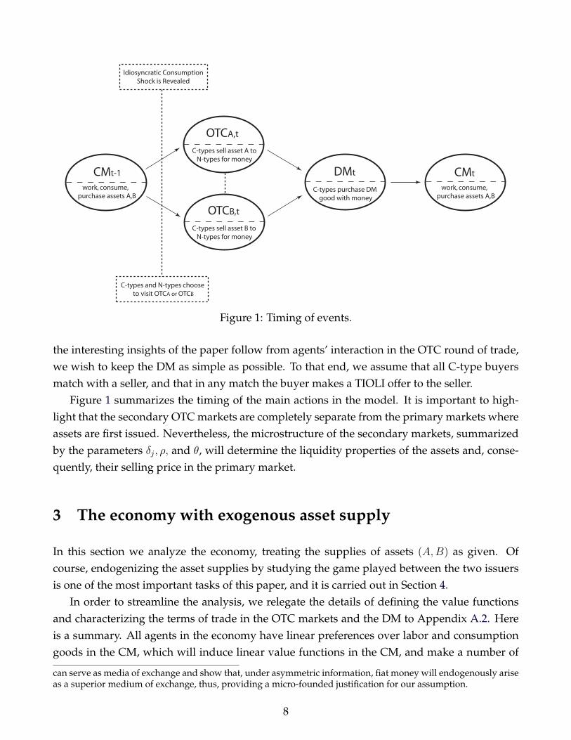
Figure 1: Timing of events.

the interesting insights of the paper follow from agents’ interaction in the OTC round of trade,we wish to keep the DM as simple as possible. To that end, we assume that all C-type buyersmatch with a seller, and that in any match the buyer makes a TIOLI offer to the seller.

Figure 1 summarizes the timing of the main actions in the model. It is important to high-light that the secondary OTC markets are completely separate from the primary markets whereassets are first issued. Nevertheless, the microstructure of the secondary markets, summarizedby the parameters δj, ρ, and θ, will determine the liquidity properties of the assets and, conse-quently, their selling price in the primary market.

3 The economy with exogenous asset supply

In this section we analyze the economy, treating the supplies of assets (A,B) as given. Ofcourse, endogenizing the asset supplies by studying the game played between the two issuersis one of the most important tasks of this paper, and it is carried out in Section 4.

In order to streamline the analysis, we relegate the details of defining the value functionsand characterizing the terms of trade in the OTC markets and the DM to Appendix A.2. Hereis a summary. All agents in the economy have linear preferences over labor and consumptiongoods in the CM, which will induce linear value functions in the CM, and make a number of

can serve as media of exchange and show that, under asymmetric information, fiat money will endogenously ariseas a superior medium of exchange, thus, providing a micro-founded justification for our assumption.

8

economic decisions easy to characterize. First, consider a DM meeting between a seller and aC-type buyer who brings a quantity m of money. Suppose the real price of money (in terms offruit) in the subsequent CM is ϕ > 0. Then the buyer will either buy the first-best quantity q∗,or, if her money is not enough, spend all of it on the quantity q = ϕm < q∗. Second, considera meeting in the OTC market for asset j ∈ A,B, where the N-type brings a quantity m ofmoney, and the C-type brings a portfolio (m, dj) of money and asset j. With probability 1 − θ,the N-type makes a TIOLI offer, in which case she buys the C-type’s assets and compensateshim with the least amount of money that the C-type will accept. With probability θ, the C-typemakes a TIOLI offer, in which case he receives the N-type’s money and compensates her withassets valued at par.15

What is the probability of matching in an OTC market for an individual agent? First, leteC∈ [0, 1] and e

N∈ [0, 1] denote the fractions of C-types and N-types, respectively, who are

choosing to enter OTCA in equilibrium. Then, the measure of asset sellers and buyers in OTCA

is given by eC` and e

N(1− `), respectively, and the measure of asset sellers and buyers in OTCB

is given by (1 − eC

)` and (1 − eN

)(1 − `). Let αij ∈ [0, 1] denote the matching probabilities (orarrival rates) for agents of type i = C,N in OTCj , j = A,B. Given that matching is random,they satisfy:

αCA ≡fA(eC`, e

N(1− `)

)eC`

, αCB ≡fB((1− e

C)`, (1− e

N)(1− `)

)(1− e

C)`

, (1)

αNA ≡fA(eC`, e

N(1− `)

)eN

(1− `), αNB ≡

fB((1− e

C)`, (1− e

N)(1− `)

)(1− e

N)(1− `)

. (2)

3.1 Optimal behavior

In this sub-section, we describe the optimal behavior of the representative buyer. As is stan-dard in models that build on LW, all buyers will choose their optimal portfolio independentlyof their trading histories in preceding markets. This result follows from the “no-wealth effects”property, which, in turn, stems from the quasilinear preferences. What is new here is that inaddition to choosing an optimal portfolio of money and assets, (m, dA, dB), buyers also choosewhich OTC market they will enter in order to sell or buy assets once their type has been re-

15 In OTC trade, three kinds of outcomes are possible: (a) the C-type’s asset holdings could limit the trade; (b)the N-type’s money holdings could limit the trade; (c) or both are so large that the pooled money is enough topurchase the first-best DM quantity (m+ m > q∗/ϕ), and the C-type has enough assets to compensate the N-type.In Geromichalos and Herrenbrueck (2016), we showed that assets can only be priced (in the CM) at a determinateliquidity premium if case (a) applies in the corresponding OTC market. Case (c) will also be relevant for thepresent paper as the boundary of case (a), where an asset becomes abundant and the liquidity premium convergesto zero. Case (b), however, only complicates the general equilibrium analysis. Since there cannot be a positiveliquidity premium in this case, and since our interest is in asset issuers who seek to exploit such a premium, weexclude case (b) from our analysis. This is done by assuming that inflation is not too large, so that all agents carryat least half of the first-best amount of money.

9

vealed. The buyer’s choice can be analyzed with an objective function, denoted by J(m, dA, dB),which summarizes the cost and benefit from choosing portfolio (m, dA, dB). To obtain J , sub-stitute the values of trading in the OTC markets and in the DM (Equations A.4-A.8, derived inthe appendix) into the maximization operator of the CM value function (Equation A.1). Afterusing the linearity of the value function itself (Equation A.2), we can drop all terms that do notdepend on the choice variables (m, dA, dB) to obtain the objective function:

J(m, dA, dB) = −ϕ(m+ pAdA + pBdB

)+ βϕ

(m+ dA + dB

)

+ β`

u (ϕm)− ϕm+ max

θαCASCA︸ ︷︷ ︸

enter A

, θαCBSCB︸ ︷︷ ︸enter B

, (3)

so that the optimal portfolio choice of buyers is fully described by max J , where the currentprices of money and assets, (ϕ, pA, pB), and the future price of money, ϕ, are taken as given.

The interpretation of the objective function is intuitive. The first term represents the costthat the buyer needs to pay in order to purchase the portfolio (m, dA, dB) in the CM, and thesecond term represents the benefit from selling these assets in the CM of the next period. If onewere to shut down the DM market (say, by setting ` = 0), there would be no liquidity consid-erations and the buyer’s objective function would consist only of these two terms. However,as indicated by the third term, the buyer may turn out to be a C-type in the next period withprobability `. In this case she can use her money (m) to purchase consumption in the DM (gen-erating a net surplus equal to u [ϕm]−ϕm), and she can enter OTCj , j = A,B, in order to acquiremore money by selling her assets (dA or dB). In the last expression, the terms SCj represent thesurplus for the C-type in OTCj , but notice that the buyer will actually enjoy this surplus only ifshe gets to match in that market and make the TIOLI offer, an event that occurs with probabilityθαCj .16 Exploiting the OTC bargaining solution (i.e., Lemma A.2) and Equation (A.9), one canverify that, for j = A,B:

SCj =

u(q∗)− u(ϕm)− q∗ + ϕm, if dj > m∗ − m,

u(ϕm+ ϕdj)− u(ϕm)− ϕdj, otherwise,(4)

where the condition dj > m∗ − m states that in this case the agent’s asset holdings are “abun-dant”, i.e., they allow her to reach the first-best amount of money, m∗, through OTC trade.

16 One may wonder why there is no (1− `)-term in the objective function. Does the N-type not generate valueby bringing money into the OTC? Yes, this is the case, as the full value function (Equation A.1) shows. But thetechnical restriction (6), justified in Footnote 15, guarantees that the N-type’s money is never marginal in OTCtrade. Hence the N-branch can be dropped from the portfolio choice problem; the only decision to be made alongthe N-branch is which OTC market to enter.

10

Having established the buyers’ objective function, two important observations are in order.First, while we have only imposed an exogenous segmentation assumption on the OTC mar-kets, an endogenous segmentation will arise in the primary markets: i.e., buyers will typicallychoose to purchase only asset A or asset B in the CM. In equilibrium, assets will trade at a pre-mium, and buyers will only pay this premium if they expect to sell the asset in the OTC. Sincethey can only enter one OTC (and anticipate having to choose eventually), they will chooseex-ante (i.e., in the CM), to “specialize” in asset A or B.17 This, in turn, implies that a buyer’sportfolio choice is intertwined with the choice of which OTC market to enter in case she turnsout to be a C-type. That is, buyers who choose to specialize in asset A will typically chooseto hold a different portfolio than those who specialize in asset B. For instance, we shall seein what follows that agents who choose to trade in a less liquid OTC market will self-insureagainst the liquidity shock by carrying more money.

The second important observation is that the buyer’s choice of which OTC market to enterif she turns out to be an N-type is unrelated with her choice of asset specialization in the CM.This follows directly from Lemma A.2, which specifies that only the asset and money holdingsof the C-type buyer matter for the bargaining solution in OTC trade. As a result, regardless ofher asset choice which by the time the N-type makes her OTC entry choice is sunk, this agentwill enter OTCA only if:

(1− θ)αNASNA ≥ (1− θ)αNBSNB.

In the last expression, the terms SNj represent the surplus for the N-type in OTCj . ExploitingLemma A.2 and equation (A.10), one can verify that, for j = A,B,

SNj =

u(q∗)− u(ϕm)− q∗ + ϕm, if dj > [u(q∗)− u(ϕm)]/ϕ ,

ϕm+ ϕdj − u−1[u(ϕm) + ϕdj

], otherwise,

(5)

where (m, dj) stand for the N-type’s expectation about the money and asset-j holdings, respec-tively, that her trading partner, a C-type, will carry into OTCj . The condition dj > [u(q∗) −u(ϕm)]/ϕ states that the asset holdings of the C-type are large enough to allow her post-OTCmoney balances to reach the first-best amount, m∗.

3.2 Equilibrium

In steady state, the cost of holding money can be summarized by the parameter i ≡ (1+µ−β)/β;exploiting the Fisher equation, this parameter represents the nominal interest rate on an illiquidasset. For example, in any equilibrium it must be true that pj ≥ 1/(1 + i), j = A,B, since

17 Buyers may still hold the other asset if indifferent, i.e., if that asset is abundant or illiquid.

11

otherwise there would be an infinite demand for the assets; however, the inequality could bestrict if the assets are liquid. The restriction µ > β− 1 translates into i > 0. We also assume that:

i < `(1− θ) [u′ (q∗/2)− 1] , (6)

a technical restriction. It ensures that q0j > q∗/2 for every buyer, thus the N-type’s money willnever be the limiting factor in OTC trade. See our explanation in Footnote 15, and note that ifwe did have q0j < q∗/2, the implied burden of the inflation tax would be enormous.

We have thirteen endogenous variables.18 First, we have the equilibrium real balanceszA, zB held by the buyer who chooses to specialize in asset A or B (recall from the discus-sion in Section 3.1 that an agent who chooses to trade in OTCA will typically make differentportfolio choices than one who chooses to trade in OTCB).

Next, we have the equilibrium quantities q0A, q1A, q0B, q1B, q1A, q1B. The first four repre-sent the quantity of DM good purchased by a C-type buyer who either did not trade in theOTC market (indexed by 0), or who traded and made the TIOLI offer (indexed by 1), depend-ing on whether they chose to specialize in asset A or asset B. The last two terms (i.e., the q’s)represent the quantity of DM good purchased by a buyer who traded in her chosen OTC, A orB, but did not get to make the TIOLI offer (because the N-type did). It is clear from Lemma A.2that the purchasing power of the C-type in the DM will depend on whether she got to make theoffer or not, and, naturally, we have q1j ≥ q1j , for all j.19

Next, we have the prices of the three assets ϕ, pA, pB. And, finally, we have the marketentry choices e

C, e

N, i.e., the fractions of C-types and N-types, respectively, who choose to

enter OTCA.We now show how seven out the thirteen endogenous variables can be derived directly

from the following six variables, q0A, q1A, q0B, q1B, eC , eN. First, it is clear that zj = q0j , forj = A,B, since the C-type who does not trade in the OTC can only purchase the amountof DM goods that her own real money holdings, zj , allow her to afford. Second, the price ofmoney solves:

ϕM = eCq0A + (1− e

C)q0B. (7)

This equation is the market clearing condition in the market for money. Third, the equilibriumasset prices must satisfy the demand equations:20

18 This count excludes the terms of trade in the OTC markets, since they follow directly from the main endoge-nous variables described in this section and Lemma A.2.

19 More precisely, we have q1j > q1j , unless the C-type’s asset holdings satisfy dj ≥ [u(q∗) − u(ϕm)]/ϕ. Then,even if the N-type makes the offer the C-type can afford a money transfer of m∗ −m, and we have q1j = q1j = q∗.

20 These follow directly from obtaining the first-order conditions in the buyer’s objective function, i.e., Equa-tion (3), and imposing equilibrium quantities. Notice that the asset prices do not only depend on the variables q1j ,but also on the equilibrium values of e

C, e

Nwhich affect the arrival rates αCj ; see Equations (1).

12

pj =1

1 + i

(1 + ` αCjθ · [u′(q1j)− 1]

), for j = A,B. (8)

For future reference, notice that as long as q1j < q∗, the marginal unit of the asset allows theagent to acquire additional money which she can use in order to boost her consumption in theDM. In this case, the agent is willing to pay a liquidity premium in order to hold the asset. Onthe other hand, if q1j = q∗, the term inside the square brackets becomes zero, and pj = 1/(1 + i),which is simply the fundamental price of a one-period nominal bond.

Finally, the quantities consumed in the DM by buyers who did not make the TIOLI offer inthe preceding OTC market satisfy:

q1A = min

q∗, u−1

(u(q0A) + ϕ

A

eC

), (9)

q1B = min

q∗, u−1

(u(q0B) + ϕ

B

1− eC

), (10)

where ϕ has been explicitly defined as a function of the variables q0j in (7). (These equationsare derived from substituting equilibrium variables into part (b) of Lemma A.2.)

The analysis so far establishes that if one had solved for q0A, q1A, q0B, q1B, eC , eN, then theremaining seven variables could also be immediately determined. Hence, hereafter we referto these six variables as the “core” variables of the model. We now turn to the description ofthe equilibrium conditions that determine the core variables. Throughout this discussion, recallthat the terms e

C, e

Nare also implicitly affecting the arrival rates αCj .

First, the money demand equation for those specializing in asset j:

i = ` (1− αCjθ) · [u′(q0j)− 1] + ` αCjθ · [u′(q1j)− 1] , for j = A,B. (11)

Note that we have defined αij = 0 if there is no entry at all into market j. If that is the case, q0jand q1j are still defined as limits even though nobody actually trades at those quantities.

Next, the OTC trading protocol links q0j and q1j . Consider for instance market A. Thebargaining solution, evaluated at equilibrium quantities, becomes:

q1A = min

q∗, q0A +

ϕA

eC

,

where ϕA/eC

stands for the real value of assets that the C-type brings into OTCA.21 Even thoughthe real aggregate supply of asset A is ϕA, the buyer under consideration holds more than the

21 If the C-type’s asset holdings are plentiful in the OTC, then we know that this agent will be able to purchasethe first-best amount of money in the DM, hence, q1A = q∗. On the other hand, if the asset is scarce in OTCtrade, the C-type gives away all of her assets, ϕA/e

C. Moreover, since here we are in the case where the C-type

makes the offer, she will swap assets for money at a one-to-one ratio. As a result, in equilibrium it must be thatq1A = q0A + ϕA/e

C, which explains the last expression.

13

average because some buyers choose not to hold asset A at all (i.e., the buyers who specializein asset B). After substituting the price of money from Equation (7) into the last expression, weobtain two equations, one for each market:

q1A = min

q∗, q0A +

A

M· eCq0A + (1− e

C)q0B

eC

, (12)

q1B = min

q∗, q0B +

B

M· eCq0A + (1− e

C)q0B

1− eC

. (13)

If it happens that eC

= 1 (no C-types enter theB-market) andB > 0, then we define q1B = q∗ as alimit, because a C-type of infinitesimal size who decided to deviate and hold assetB could holdthe entire stock of it, which would certainly satiate them in an OTC trade – in the hypotheticalcase that there was an N-type in the B-market willing to trade with them. Similarly, if e

C= 0

and A > 0, then we define q1A = q∗.How large can the aggregate supply of an asset be for the asset to remain scarce in OTC

trades? Clearly, the asset is more likely to be scarce if its ownership is diluted, i.e., if manybuyers choose to hold that asset in the CM. So for example, asset A is most likely to be scarce ifeC

= 1. But in this special case, Equation (12) tells us that the asset is scarce (q1A < q∗) only if thecondition 1 + A/M < q∗/q0A is satisfied. On the boundary, q1A = q∗, so we can use the moneydemand equation (11) to obtain the bounds:

A ≡M (q∗/q0A − 1) , where q0A solves i = [`− θ fA(`, 1− `)] [u′(q0A)− 1] ,

B ≡M (q∗/q0B − 1) , where q0B solves i = [`− θ fB(`, 1− `)] [u′(q0B)− 1] .

There are three things to notice here. First, if A > A, then asset A is certain to be abundant butthe reverse is not always true, because asset ownership can be concentrated in the hands of a fewbuyers. Second, if we did fix e

C= 1 so that ownership of asset A was maximally diluted, then

asset A would indeed be abundant if and only if A ≥ A, and conversely for asset B. Third, ifthe market for asset A has an exogenous liquidity advantage (δA > δB), then A > B, and viceversa. In order to have a term for the maximal upper bound on asset supply beyond whicheither asset is certain to be abundant, we define:

D ≡ maxA, B.

The remaining task is to characterize the OTC market entry choices. Consider first a C-type.As we have already discussed, this type at the beginning of the period has already made thechoice to hold either asset A or asset B, so the choice of which market to enter has effectivelybeen made. The critical choice takes place in the preceding CM, where the agent chooses whichasset to specialize in. Evaluating equation (4) at equilibrium quantities, we find that if the C-

14

type makes the TIOLI offer, her surplus of trading in market j ∈ A,B equals:22

SCj = u(q1j)− u(q0j)− q1j + q0j. (14)

But since the buyer’s portfolio choice effectively determines her market choice if she turns outto be a C-type, this surplus has to be balanced not only against the probability of matching, αCj ,and the probability of making the offer, θ, but also against the cost of carrying the asset in thefirst place. Hence, we define the “net” surplus that the buyer obtains if she chooses to specializein asset j to be:

SCj ≡ −iq0j − [(1 + i)pj − 1](q1j − q0j) + αCjθSCj.

We can use the money and asset demand equations (8 and 11) to substitute for i and pj in thelast expression. After some algebra, we obtain:

SCj = (1− αCjθ) · [u(q0j)− u′(q0j)q0j] + αCjθ · [u(q1j)− u′(q1j)q1j] . (15)

Thus, in equilibrium, the C-types’ portfolio choice eC

must satisfy:

eC

=

1, if SCA > SCB,

0, if SCA < SCB,

∈ [0, 1], if SCA = SCB.

(16)

Finally, we want to characterize the market choice of the N-type buyers. Since these agentsare asset buyers, their own asset holdings do not matter, so they can enter the market for eitherasset independently of which asset they chose to hold in the preceding CM. Thus, an N-typewill simply enter the market in which she expects a greater surplus, accounting for the proba-bility of trading and making the TIOLI offer. Evaluating equation (5) at equilibrium quantitiesimplies that the surplus for the N-type who chooses to enter OTCA is given by:

SNA =

u(q∗)− u(q0A)− q∗ + q0A, if A/e

C> [u(q∗)− u(q0A)]/ϕ ,

q0A + ϕ AeC− u−1

(ϕ AeC

+ u(q0A)), otherwise,

(17)

22 This equality holds regardless of whether the asset is plentiful in the OTC meeting or not. Consider firstthe case of plentiful assets. For this case evaluating the relevant (i.e., the “abundant”) branch of equation (4) atequilibrium quantities yields SCj = u(q∗) − u(q0j) − q∗ + q0j , which is exactly what one would obtain if q1j = q∗

was imposed on equation (14). Next, consider the case of scarce assets and for simplicity focus on OTCA. In thiscase, evaluating (4) at equilibrium quantities yields SCj = u(q1j)− u(q0j)− ϕA/eC , where ϕA/e

Cis the real value

of assets that the C-type brings into OTCA. But as we know from the discussion that leads to equation (12), hereq1A = q0A + ϕA/e

C. Hence, the validity of equation (14) is once again verified.

15

and the surplus for the N-type who chooses to enter OTCB is given by:

SNB =

u(q∗)− u(q0B)− q∗ + q0B, if B/(1− e

C) > [u(q∗)− u(q0B)]/ϕ ,

q0B + ϕ B1−e

C− u−1

(ϕ B

1−eC

+ u(q0B)), otherwise.

(18)

In (17) and (18) we have used the value of money, ϕ, to keep these expressions relatively short,but it is understood that ϕ is itself a function of the core variables, defined in (7).

Thus, in equilibrium, the N-types’ entry choice eN

must satisfy:

eN

=

1, if αNASNA > αNASNB,

0, if αNASNA < αNASNB,

∈ [0, 1], if αNASNA = αNBSNB.

(19)

We can now define a steady state equilibrium in the model with fixed asset supplies:

Definition 1. Assume (for now) that asset supplies are fixed and equal to (A,B) ∈ R+ × R+.A steady state equilibrium for the core variables of the model is a list q0A, q1A, q0B, q1B, eC , eNsuch that Equations (11) for j = A,B, (12), and (13) hold, and buyers’ entry choices satisfyEquations (16) and (19).

3.3 Structure of equilibrium

We are now ready to construct the equilibria of the economy, summarized by the core variablesq0A, q1A, q0B, q1B, eC , eN, conditional on the asset supplies A,B ≥ 0. As we show below, thesystem admits a closed form solution in one special case, which we call “balanced CRS”: thereare CRS in OTC market matching (ρ = 0) and neither asset has an exogenous liquidity advan-tage (δA = δB).23 However, a general analytical characterization is not possible, and the rest ofthe analysis will therefore be numerical. (The model can also not be simplified without losingessential insights.24) In order to understand the nature of the possible equilibria, it is instructive

23 We use the word “balanced” to describe the situation where δA = δB . We could also call it “symmetric”, butwe reserve that word for equilibria where all variables indexed by A equal their B-counterparts (e.g., pA = pB).Notice that even in the balanced environment, there are asymmetric equilibria.

24 We have a core system of six equations, and most of the endogenous variables show up in multiple equations.Moreover, the equations are non-linear and include kinks, due to the various branches that characterize the agents’market entry decisions. One may wonder whether some simplifying assumptions would allow us to achieve ananalytical characterization. We believe that the model presented here constitutes the most parsimonious frame-work that can capture all the salient features of the question we are studying, hence, any further simplificationwould eliminate insights that we think are essential. A few examples may clarify this point. A simplifying as-sumption often adopted in these types of models is that the bargaining power of agents is equal to either 0 or 1.(This is precisely what we assume for the DM, because not many interesting things happen in that market.) Im-posing such an assumption in the OTC would be a bad idea: it would imply that either the C-types or the N -types

16

0.2 0.4 0.6 0.8 1.0eN

-1.0

-0.5

0.5

1.0

high B, low A

0.2 0.4 0.6 0.8 1.0eN

-1.0

-0.5

0.5

1.0

high A, low B

0.2 0.4 0.6 0.8 1.0eN

-1.0

-0.5

0.5

1.0 Ρ = 0

low A,B

0.2 0.4 0.6 0.8 1.0eN

-1.0

-0.5

0.5

1.0

high A, B0.2 0.4 0.6 0.8 1.0

eN

-1.0

-0.5

0.5

1.0 Ρ = 0

low A,B

Figure 2: The function G(eN

) for CRS (ρ = 0) and varying asset supplies.

to start with the following exercise: first, we fix a level of eN

(the proportion of N-types whoenter theA-market), then we compute the optimal portfolio choices through Equations (11)-(13)and (16), and finally, we compute the function:

G(eN

) =αNASNA − αNBSNBαNASNA + αNBSNB

,

where all the S- and α-terms have the optimal choices substituted. So the function G(eN

) mea-sures the relative benefit to an individual N-type buyer from choosing the A-market over theB-market, assuming a proportion e

Nof all other N-type buyers enters the A-market, and all

other decisions are conditionally optimal. To make it easier to visualize, G is scaled to lie be-tween -1 and +1.

Figures 2 and 3 show how this relative return depends on eN

, for different values of ρ. In allcases, a high e

Ncauses a high value of e

C, too; when there are many buyers in an asset market,

sellers would like to go to the same market. Of course, nobody would try to trade in a ghosttown, so it must be the case that e

C= 0 if and only if e

N= 0, and e

C= 1 if and only if e

N= 1.

Therefore, the corners are always equilibria. If eN

= eC

= 0, then G(eN

) = −1, so indeed allN-types prefer the B-market; and if e

N= e

C= 1, then G(e

N) = +1, so all N-types prefer the

A-market, and nobody would want to deviate.However, the interior equilibria with e

N∈ (0, 1) are more interesting than the corners. Our

claim is that with CRS and small enough asset supplies, as eN

becomes relatively large an in-dividual N-type will prefer to deviate and enter the B-market. This may seem puzzling – thematching function exhibits CRS, so why are there not many equilibria with constant markettightness? This is indeed true, but only when asset supplies are large enough so that each in-

get no surplus from OTC trade, which would render their entry decision indeterminate. As we have explained,the agent’s decision about which market to visit is one of the most important economic forces in our model. Asanother example, some papers (e.g., Mattesini and Nosal, 2015) gain tractability by assuming that asset trade takesplace only in OTC markets, and the original asset holdings are given to agents in the CM as endowments, i.e.,there is no primary asset market. Clearly, such an assumption here would deprive the model of its most importantingredient: the endogenous determination of asset supply.

17

dividual C-type is carrying enough assets to obtain the first-best quantity of money in case sheis matched and makes the offer. The right panel of Figure 2 shows just such a continuum ofequilibria for e

N∈ [0.2, 0.8].

When asset supplies are small enough, on the other hand, there is a general equilibriumeffect: concentration or dilution of the asset portfolios as e

Cchanges. If many C-types hold the

A-asset, and the supply of A is not too large, then each of them will hold only a small amount,which implies a small individual trading surplus in the A-market and a larger individual trad-ing surplus in theB-market. It is for this reason that the curves in the left panel of Figure 2 slopedown. If many N-types were to enter the A-market, many C-types would follow; but each ofthese C-types would hold a small quantity of the A-asset, trading returns would be poor in thatmarket, and therefore an individual N-type would be better off switching to the B-market. Infact, with CRS and small asset supplies, there is a unique interior equilibrium and it is stable inthe sense that if a small proportion of N-type agents makes a mistake and enters the ‘wrong’market, everybody else’s best response would be to switch until the equilibrium proportionsare restored. This is not true at the corners.25

Everything else equal, N-types are more likely to enter the A-market if: (i) δA > δB, becausethen the A-market has an exogenous matching advantage; (ii) A > B, because then there is alarger potential surplus when trading asset A; (iii) e

Cis large, because the more C-types enter

the A-market, the easier it becomes for N-types to match; and (iv), if eN

is small, which reducesthe congestion between N-types in the A-market. Analogous considerations apply for the C-types. Consequently, a larger supply of an asset shifts everybody’s entry choices towards themarket for that asset – up to the point where the asset becomes abundant, in the sense that theindividual C-types’ need for money is satiated after selling that asset in the OTC.

The entry choice is more complex when there are increasing returns to matching in the OTCmarkets. For example, the left panel of Figure 3 shows an intermediate amount of increasingreturns, ρ = 0.5. In this case, both C- and N-types would prefer to trade in a thicker market.In the figure, there are five equilibria: the two corners (which are both stable now in the senseof being robust to small errors), the stable interior equilibrium, and two unstable asymmetricequilibria. With strongly increasing returns, ρ = 1, the picture has completely reversed: agentsso strongly prefer to be in the thicker market that this dominates the dilution of asset portfolios.The corners are now the only stable equilibria; there exists an interior equilibrium by continu-ity, but if it was ever played, a small variation in any parameter of the model would drive thebuyers into one of the corners.

25 Hence, despite coordination being important here, this is not the standard “coordination game” from thegame theory textbook. In that game, the mixed strategy equilibrium involves a coordination failure, and the cor-ners represent coordination success. Here, this is true only when the matching function exhibits increasing returns(most strongly so if ρ = 1). With constant returns, the matching probability is determined by market tightness,not by the total measure of entrants. If we held gains from trade fixed, there would always be a continuum ofequilibria with e

C= e

N, including the corners and every probability in between. What we call “asset dilution” is

just saying that gains from trade are not fixed.

18

0.2 0.4 0.6 0.8 1.0eN

-1.0

-0.5

0.5

1.0 Ρ = 0.5

0.2 0.4 0.6 0.8 1.0eN

-1.0

-0.5

0.5

1.0 Ρ = 1

Figure 3: The function G(eN

) given different degrees of IRS in matching; in both figures wehave A+B < D so that there is an overall scarcity of liquidity.

Throughout the rest of the paper, we compute equilibria as follows. We maintain the pa-rameters u = log, ` = 0.5, θ = 0.5, i = 0.1, and M = 1, which yield A = 0.8/(4 − δA) andB = 0.8/(4 − δB). In the rest of Section 3, we vary the asset supplies A and B as described ineach case, and in Section 4, the asset supplies will be chosen endogenously. Throughout, wevary the parameters of OTC microstructure (δA, δB, ρ) as described in each case. With this set ofparameters, we guess a starting point for e

N, then iterate the function G(e

N) in the direction of

its sign, until convergence or until reaching a corner. If the corners are not stable, this procedurewill always find an interior equilibrium. On the other hand, a stable interior equilibrium mayexist but not be found if a corner is stable and the starting point is close to it.26

3.4 Characterization of equilibria

Now that we understand the structure of possible equilibria, we want to compare asset pricesin these equilibria, and interpret the comparative statics of prices with respect to quantities asthe aggregate demand for these assets. These comparative statics are shown in Figure 4. In allgraphs, the supply of asset A is on the horizontal axis and the supply of B is held fixed andindicated by a gray vertical line. We show three cases: first, the simplest case of balanced CRS(ρ = 0 and δA = δB); second, giving an exogenous advantage to asset A (δA > δB); and third,without an advantage for either asset but with IRS in matching (ρ > 0). In all three examples,the graphs in the top row show the net liquidity premia of assets A and B, defined as:

Lj ≡ (1 + i)pj − 1 = ` αCjθ [u′(q1j)− 1] .

26 To be specific: we iterate G on the starting point e0N≡ δAA/(δAA+ δBB), since if a stable interior equilibrium

exists, it is likely to involve more entry into the market with a higher matching probability, and/or higher tradingvolume. There are other realistic assumptions: suppose trade was concentrated at one corner in recent periods,then this corner will likely have an advantage in being selected again. But strategic dependence over time isbeyond the scope of our analysis here.

19

“Balanced CRS”: “Unbalanced CRS”: “Balanced IRS”:ρ = 0, δA = δB = 1 ρ = 0, δA = 1, δB = 0.9 ρ = 0.25, δA = δB = 1

0 B0.1 0.2A0

1

2

LALB =

0 B0.1 0.2A0

1

eC eN=

0 B0.1 0.2A0

1

2

LALB

0 B0.1 0.2A0

1

eC

eN

0 B0.1 0.2A0

1

2

LA

LB

0 B0.1 0.2A0

1

eC

eN

Figure 4: Net liquidity premia Lj (in %) and entry choices, varying A and holding B fixed(indicated by a vertical line).

The graphs in the bottom row of the figure show the market entry choices eC

and eN

.Notice first that some standard results are replicated in our model. First, the liquidity pre-

mium of an asset is zero if that asset is in very large supply, no matter how liquid the marketfor that asset is. The reason is that as the asset supply becomes large enough, q1j → 1. (Oneshould be careful with the terms here: the asset does not “lose” its liquidity properties in thatcase, they only become inframarginal. The asset still contributes to the overall supply of liquid-ity in the sense that money demand will be lower than it would be if that asset did not exist.)Furthermore, real balances decrease with inflation so the need to liquidate assets in the OTCmarkets becomes stronger with inflation; if the asset supplies are small enough, the liquiditypremium on any liquid asset will rise with inflation, too.

In addition to these standard results, our model also delivers new insights into asset pric-ing in this environment of segmented OTC markets. Three results stand out. The first is thatwhen matching in the markets exhibits “balanced CRS” (that is, CRS and neither market has anexogenous liquidity advantage), there exists a unique interior equilibrium when the asset sup-plies are not too large. In this equilibrium, e

C= e

N= A/(A+B), so the ratio of buyers to sellers

is 1 in each market, and the assets turn out to be perfect substitutes: we have pA = pB and allthe equilibrium quantities and prices only depend on the sum of the asset supplies, A+B. Theleftmost column of Figure 4 illustrates this.

The second result from this section is that exogenous liquidity differences are amplified bythe market entry process, even with CRS. Consider a case where δA > δB, so that OTCA has anexogenous liquidity advantage. As illustrated in the middle column of Figure 4, both e

Cand e

N

increase, but the latter increases more. Intuitively, the N-types only consider the potential trad-

20

ing surplus in the OTC market when deciding which market to enter, while the C-types alsoconsider the ex-ante cost of carrying either asset, and therefore the N-types are more sensitive toliquidity differences when choosing their market. The end result is that market tightness fromthe point of view of asset sellers rises in the more liquid market and falls in the less liquid one:formally, we observe that the elasticity of the endogenous ratio αCA/αCB with respect to theexogenous ratio δA/δB is bigger than 1. Crucially, it is the point of view of OTC asset sellers thatmatters for asset pricing at the issue stage; people who buy a newly issued asset are concernedabout the conditions at which they can sell it down the road, but people who plan to buy theasset later in the secondary market have no influence on the issue price. As a consequence, evena small divergence of δA and δB will drive a larger wedge between the liquidity premia on thetwo assets. We view this result as the first step of an explanation why two assets with otherwisesimilar features can have big differences in their liquidity – most prominently, of course, U.S.Treasuries compared to equally safe corporate or municipal bonds.

The third result from this section is that IRS in matching encourage market concentration,i.e., corner equilibria. This is illustrated in the rightmost column of Figure 4. Near the origin,we have a case ofA B, so assetA is barely traded in OTC markets (though not entirely absentdue to the fact that ownership of asset B is much more diluted). As the supply of A increases,more agents are willing to trade it in the OTC market because of the increase in potential trad-ing surplus; and crucially, N-types are more sensitive to this increase, so the ratio e

N/e

Crises as

A increases. This is important because again, it means that assetA becomes rapidly more attrac-tive to C-types through two channels (market tightness and IRS).27 As asset demand in the CMby future C-types determines the issue price, the resulting increase in liquidity is so strong thatit makes the price of asset A upward sloping in its supply – at least, until that supply is so largethat the force of diminishing marginal utility takes over. But we are not done. When the supplyofA becomes even larger, all OTC trade becomes concentrated in the market forA andB ceasesto be liquid at all. As this happens, the price of asset A jumps upward discontinuously; later,we will see that this effect of increasing returns provides a powerful incentive to the issuer ofan asset to issue up to the point where competing assets are driven out of secondary markets.

There are three empirically relevant aspects of this theoretical result. First and most obvi-ously, the upward sloping demand finds its counterpart in the observation that bond liquiditycan be positively related to bond supply, which is well-established in the empirical literatureon corporate bonds (Hotchkiss and Jostova, 2007; Alexander et al., 2000).

Second, this result provides the second step of our explanation why two assets with oth-erwise similar features can have big differences in their liquidity. Even with a modest degreeof IRS in matching, an asset in smaller supply is likely to be significantly less liquid than onewhich is in larger supply, as agents prefer to enter the market where gains from trade are larger,

27 To be precise: with IRS and δA = δB , we observe eC< e

Nin the interior if and only if A < B. The more

plentiful asset is more liquid.

21

and through their own entry help to make this market “thick”. And consider how this wouldinteract with the first step described above: even with a small exogenous difference in mar-ket efficiency, the disadvantaged market is likely to see significantly less entry, and therebybecomes very “thin” indeed. In the next section, we will see how these factors reinforce oneanother, and how they interact with an endogenous choice of supply.

Third, the result can help explain how consolidating secondary markets would be beneficialfor asset issuers, a belief commonly held among practitioners (BlackRock, 2014). To see this,consider a version of our model with three issuers, A, B, and C. Compare the case where allbonds trade in distinct secondary markets with an alternative case where the OTC markets forbonds B and C merge. In our model, this would imply that, with even slight IRS in matching,the liquidity premium on bonds B and C will be higher in the second scenario, because theconsolidation of the markets reduces the investors’ risk of not being able to sell.

To summarize our results: we find that liquidity premia are always zero if asset supply islarge but may be positive if asset supply is small enough. With CRS, the liquidity premiumon a particular asset is always decreasing in that same asset’s supply; but with IRS, liquiditydepends positively on issue size and asset demand curves can therefore have upward slopingsegments. However, the liquidity premium on an asset is always decreasing in the supply ofother assets, which opens the door to strategic interaction.

4 The economy with strategically chosen asset supply

4.1 The game between the asset issuers

We look at the non-cooperative game between two issuers who seek to maximize their utility.They live only in the CM, where they can work, consume, and issue assets. Their utility withinthe period is Y(X,H) = X − H , where X,H denote consumption and work effort, and theydiscount the future by the same factor β as all agents. They take into account that the real priceat which they can sell their asset, ϕpj , depends on the supplies of both assets. For example, theproblem of issuer A who has issued A− assets in the previous period can be described by thefollowing Bellman equation:

WA(A−) = maxX,H,A

X −H + βWA(A)

s.t. X + ϕA− = H + ϕpAA,

which we can simplify to yield:

22

WA(A−) = −ϕA− + maxA

ϕpAA+ βWA(A)

.

Just like for private agents, the issuer’s choice of A does not depend on their previous choices.We can use this, plus the fact that in steady state ϕ/ϕ = (1 +µ), to solve for issuer A’s objective:

JA =ϕ

1 + i[(1 + i)pA − 1]A

=ϕ

1 + i

(` αCAθ [u′(q1A)− 1]

)A. (20)

With an analogous derivation, issuer B’s objective is:

JB =ϕ

1 + i

(` αCBθ [u′(q1B)− 1]

)B. (21)

Simply put, each issuer seeks to maximize the product of the net liquidity premium Lj and thesupply of their asset, taking into account that their choice of asset supply affects the generalequilibrium choices of the buyers.

The next step is to choose a solution concept for the game between the issuers, which is nota trivial question because there are many options. The simplest option is to model the interac-tion between the issuers as a static game, ignoring the possibility that these issuers interact inrepeated periods. The simplest static equilibrium concept is Nash equilibrium, but even withinthe static framework, there are alternatives that might be relevant in our context. For example,if one of the issuers has the ability to commit to an issue size before the other, then the ap-propriate equilibrium concept would be Stackelberg rather than Nash. In particular, this mayapply to political agents (such as the U.S. Treasury) for whom liquidity rent will not be the onlyconsideration.

And if we take the repeated interaction seriously, there are even more possibilities. For one,folk theorems would support many outcomes that are not equilibria of the stage game, includ-ing collusion. To complicate things even further, we have multiple equilibria in the stage game,but is it realistic to think that all of them could be played independently of previous outcomes?For example, say that the OTC traders played the corner equilibrium of e

C= e

N= 1 in the

last twenty periods, and say that issuer A issued a positive quantity but less than D. If issuerB were to issue a larger quantity B > A, then the OTC traders might be collectively better offto switch to an interior equilibrium or even to the B-corner. But could the traders realisticallycoordinate in this way given the recent history of A being the only asset with a liquid market?If the answer is “no”, then asset issuers in a given period would be competing not only forcurrent profits, but also for future monopolies.

Given the many doors one could open here, the analysis in this section will proceed in twoparts that should be understood as distinct. First, we will describe the payoff structure facingthe asset issuers in the stage game and analyze how this structure depends on parameters such

23

as whether one of the assets has an exogenous liquidity advantage (δA, δB), and whether thematching function exhibits CRS or IRS (ρ). We believe this will allow our readers to extrapo-late what kind of outcomes one might obtain with their preferred solution concept, whetherstatic Stackelberg or dynamic triggers. Second, for the sake of concreteness, we will solve forstatic Nash equilibria of the stage game and analyze how these equilibria, as well as resultingmacroeconomic outcomes and welfare, depend on the market parameters.28

4.2 Strategic structure of the game

In this subsection, we analyze the strategic structure of the game and the incentives asset issuersface; in the next subsection, we will analyze how static Nash equilibria of the game depend onvariations of this structure.

First, consider an economy with “balanced CRS” in financial markets (ρ = 0 and δA = δB).As we saw in Section 3.3 above, the two corner equilibria are not robust to small errors: if anarbitrarily small measure of C-types happens to enter a market with no N-types, then N-typescan profitably deviate by entering that market. As illustrated in Figure 2, more and more buyers(C and N) will enter that market until the interior equilibrium is reached; consequently, in thecase of balanced CRS, the interior equilibrium is the interesting one to study.

Using the guess-and-verify method, it is easy to show that eC

= eN

= A/(A + B) togetherwith q0A = q0B and q1A = q1B satisfies all of the equilibrium equations, and that this is theunique solution when the sum A + B is small enough. In that case, we also have q1j < q∗,and the net liquidity premia LA = LB > 0 depend only on the sum A + B: the assets areperfect substitutes and are priced along a common demand curve. This case of balanced CRSis therefore isomorphic to a version of the model where the assets could be traded in the sameOTC market rather than in segmented markets as we assume here. And because the assets areperfect substitutes (and as long as the inverse demand curve Lj(A + B) is not too convex), theonly Nash equilibrium of the game between the issuers is the symmetric Cournot equilibriumwhere both assets are issued in the same quantity, each approximately one-third of the quantityD that would drive the liquidity premium to zero.

Second, we are interested in how an economy with CRS in financial markets is affected byexogenous liquidity differences. Specifically, we set δA equal to 1 and let δB vary. The results areillustrated in Figure 5; the leftmost column illustrates the balanced CRS case, and the rightmostcolumn illustrates how if asset B has too much of a disadvantage, then the interior equilibriumof OTC market entry ceases to exist. Issuer A issues the monopoly quantity, approximatelyone-half of D, and issuer B issues an arbitrary amount because asset B is illiquid in any case.

The intermediate values of δB are the most interesting. If δB is close to but below δA, then the28 For readers who are interested, we also analyze a “semi-strategic” case where the supply of A is fixed, and B

best-responds to it. See Appendix A.3.

24

δB = 1 δB = 0.99 δB = 0.9 δB = 0.6

A’spayoff

B’spayoff

AB

A

BA

BA

B

A

B

A

B

A

B

A

B

Figure 5: Payoffs as functions of asset supplies, with CRS (ρ = 0) and asset A having an ex-ogenous liquidity advantage over asset B (δB ≤ δA = 1). Darker shades of red indicate largerpayoffs, white indicates zero. The blue and green dots indicate particular Nash equilibria.

demand curve for asset A has a kink as shown in the middle column of Figure 4. As long as δBis large enough, the Cournot equilibrium survives, though it shifts very slightly to be biased infavor ofA issuing more and receiving a larger payoff. When δB becomes smaller, however, thenA may prefer to issue a very large quantity that would concentrate OTC trade in the A-marketand drive B’s liquidity premium to zero. In this equilibrium, despite receiving a zero payoff, Bdoes not issue an arbitrary amount: if B issues too little, A would have an incentive to issue the(smaller) monopoly quantity, in which case B has an incentive to issue more, so this is not anequilibrium. We will analyze the consequences for the economy in more detail later, but we canalready see that the total supply of liquid assets is largest if B is somewhat illiquid, smallest ifB is very illiquid, and in between if both A and B are very liquid.

To summarize: with CRS in financial markets, the structure of the game resembles Cournotcompetition. If not too unbalanced, CRS supports the interior equilibrium in OTC marketswhere every asset is somewhat liquid. We see relatively low issue sizes, and we can extrapolatethat they would be larger with Stackelberg replacing Nash, and smaller if the issuers collude.

As the third case, we analyze how an economy without exogenous liquidity differences isaffected by IRS in financial markets. Specifically, we set δA = δB = 1 and let ρ vary. The resultsare illustrated in Figure 6; the leftmost column shows the balanced CRS case, and the rightmostcolumn illustrates how a strong degree of IRS makes the symmetric interior equilibrium sounstable that it effectively ceases to exist. In the latter case, the returns to issuing more than one’scompetitor become enormous because buyers strongly prefer to trade only in one market.29

Consequently, there is a (numerically approximate) Nash equilibrium where quantity A is so

29 And when computing equilibria, we made the tie-breaking assumption that buyers are more likely to pickthe corner of the asset of which there is a larger supply. See the discussion at the end of Section 3.3.

25

ρ = 0 ρ = 0.01 ρ = 0.05 ρ = 0.5

A’spayoff

B’spayoff

AB

A

BA

BA

B

A

B

A

B

A

B

A

B

Figure 6: Payoffs as functions of asset supplies, with IRS but no exogenous liquidity advantage(δA = δB = 1). Darker shades of red indicate larger payoffs, white indicates zero. The green andblue dots indicate particular Nash equilibria.

close to D that issuer B does not find it profitable to issue any more, because in either casetheir asset would trade at a zero liquidity premium, either due to being illiquid or due to beingplentiful. And there is another Nash equilibrium with A and B’s roles reversed.

Letting ρ increase smoothly, we see a smooth transformation of the playing field, too. Forlow ρ, assets tend to be strategic substitutes where players prefer to issuer neither too little nortoo much, but for high ρ, assets become strategic complements where players strongly preferto issue more than the other. Correspondingly, we see a transition from Cournot-type equilibriaof low issue sizes and both assets being liquid to asymmetric equilibria of high issue sizes andonly one asset being liquid – and this change is not smooth, but happens all of a sudden arounda critical value of ρ.

We can say that with a large enough degree of IRS in financial markets, despite being agame in quantities rather than prices, the strategic structure of the game resembles Bertrandcompetition rather than Cournot. This promotes corner equilibria, where one asset ends upbeing very liquid and the other one not liquid at all. In such equilibria, the ‘winning’ (liquid)asset must be in very large supply (close to D); however, this might not be robust to a richermodel of dynamic competition. One could imagine that if issuer A succeeds in concentratingtrade in the A-corner for enough periods, buyers might eventually form a habit of selecting theA-corner no matter how much B issues. This would permit A to issue the monopoly quantity(approximately D/2) from that point on.

26

0.6 0.7 0.8 0.9 1.0∆B0

20

40

60

80

H% of AL

A

B

0.6 0.7 0.8 0.9 1.0∆B0.0

0.2

0.4

0.6

0.8

1.0

1.2H%L

LA

LB

[a] Asset supplies [b] Net liquidity premia

0.6 0.7 0.8 0.9 1.0∆B

80

85

90

95

100H% of q*L

q0 A

q1 A

q0 B

q1 B

q

0.6 0.7 0.8 0.9 1.0∆B

0.35

0.40

0.45

0.50

0.55ΑCA

ΑCB

H1-L∆A

H1-L∆B

[c] Quantities traded in DM, and average [d] OTC matching probabilities

Figure 7: Comparative statics of the strategic equilibria with respect to δB, with CRS (ρ = 0).

4.3 Comparative statics

In this section, we analyze the comparative statics, with respect to δB, of the static Nash equilib-ria of the game between the issuers. We consider both constant returns in matching and smallamounts of increasing returns. Our goal is to understand what happens if one of the assets (Afor concreteness) has an exogenous liquidity advantage, and how the answer to this questioninteracts with the returns to scale in matching. Throughout this section, we hold δA = 1 fixed.

One thing to be aware of is how we compute the Nash equilibria. We iterate best responsesof the two issuers on a finite grid of possible asset supplies which excludes asset supplies whichwe know can never give positive payoffs: zero and supplies exceeding D. The starting point isthe smallest positive asset supply on the grid (e.g., the point (0.05D, 0.05D) on a 20×20-grid).The remaining choice is whether we let A or B move first; in this section, all equilibria are com-puted with A moving first.30

The comparative statics with CRS (ρ = 0) are illustrated in Figure 7. As δB declines slightlyfrom 1 (the balanced case), A begins to issue more and B begins to issue less (panel [a]), but the

30 The equilibria where B moves first are usually identical or payoff-identical. In Figures 5 and 6, Nash Equi-libria where A moves first are indicated with a blue dot, and those where B moves first are indicated with a greendot. Our method for computing the portfolio choices of private agents is described in Section 3.3.

27

0.6 0.7 0.8 0.9 1.0∆B0

20

40

60

80

H% of AL

A

B

0.6 0.7 0.8 0.9 1.0∆B0.0

0.2

0.4

0.6

0.8

1.0

1.2H%L

LA

LB

[a] Asset supplies [b] Net liquidity premia

0.6 0.7 0.8 0.9 1.0∆B

80

85

90

95

100H% of q*L

q0 A

q1 A

q0 B

q1 B

q

0.6 0.7 0.8 0.9 1.0∆B

0.35

0.40

0.45

0.50

0.55ΑCA

ΑCB

H1-L∆A

H1-L∆B

[c] Quantities traded in DM, and average [d] OTC matching probabilities

Figure 8: Comparative statics with respect to δB, with just the tiniest bit of IRS (ρ = 0.01).

strategic pattern of a Cournot game is maintained. The exogenous liquidity advantage of assetA is magnified by the entry choices of agents (panel [d]), which feeds back into a rising liquiditypremium on asset A and a falling liquidity premium on asset B (panel [b]). Outputs diverge:C-types who hold asset A end up purchasing smaller quantities q0A and q1A, but the probabilitythat they will obtain the larger one of the two, q1A, increases. Conversely, C-types who still holdasset B despite its liquidity disadvantage are compensated with higher quantities q0B and q1B

(panel [c]).As δB declines further, we observe a discontinuity. At some point, the benefit to A from

ramping up the issue size all the way to drive out B from the financial markets becomes toostrong, so this is what A does. Asset B becomes fully illiquid, and therefore its issue size andthe quantities q0B and q1B become indeterminate. As a result of this aggressive competition,average output of DM goods is highest at the discontinuity. If δB declines even more, the threatof trading asset B gradually diminishes; eventually, A becomes a monopolist who issues anintermediate quantity of asset A and average output declines to its lowest value. (Welfare is amore complicated story, as we explain in Section 4.4 below.)

When we allow for a very small degree of IRS in matching, ρ = 0.01 (illustrated in Figure 8),the results are almost identical to those with CRS, as one might expect given that ρ is so close to

28

0.6 0.7 0.8 0.9 1.0∆B0

20

40

60

80

H% of ALA

HB undeterminedL

0.6 0.7 0.8 0.9 1.0∆B0.0

0.2

0.4

0.6

0.8

1.0

1.2H%L

LA

LB

[a] Asset supplies [b] Net liquidity premia

0.6 0.7 0.8 0.9 1.0∆B

80

85

90

95

100H% of q*L

q0 A

q1 AHq0 B, q1 B

undeterminedL

q

0.6 0.7 0.8 0.9 1.0∆B

0.35

0.40

0.45

0.50

0.55ΑCA

ΑCB

= H1-L∆A

H1-L∆B

[c] Quantities traded in DM, and average [d] OTC matching probabilities

Figure 9: Comparative statics with respect to δB, with a little bit more IRS (ρ = 0.02).

zero. Even so, we can see that the transition from the interior equilibrium to theA-corner whereasset B is illiquid happens ‘sooner’, i.e., for a higher value of δB, than under CRS. Increasingreturns make it slightly easier for A to drive B out of the market: in the example, A will do sofor δB = 0.87 under ρ = 0.01 but not under ρ = 0.

Based on Figure 6, one would guess that when increasing returns are strong enough, theCournot-style equilibrium is eliminated in favor of aggressive competition for secondary mar-ket liquidity. But how strong do they need to be? Our perhaps surprising answer is: not very.In fact, as Figure 9 illustrates, the transition occurs somewhere between ρ = 0.01 and ρ = 0.02;in the latter case, even with a relatively tiny degree of IRS, competition for liquidity is fierceand only one market is open in all strategic equilibria. However, this does not mean that theexogenous liquidity parameter δB stops mattering. When δB = δA = 1, an issuer who wishes tocapture the secondary market must issue the quantity D, which also drives her own payoff tozero. But as δB declines, so does the threat ofB’s competition. As a consequence, as δB declines,the equilibrium asset supply A falls. Ultimately, the quantity q1A of DM trade for C-types whotraded at full surplus in the OTC market also falls but the quantity q0A of DM trade for C-typeswho did not trade rises (because agents self-insure against the lower trading surplus by holdingmore money). On balance, and in our numerical example, the effect on q1A dominates so that

29

0.6 0.7 0.8 0.9 1.0∆B-1.30

-1.29

-1.28

-1.27

-1.26

-1.25

-1.24

H%L

0.6 0.7 0.8 0.9 1.0∆B-1.30

-1.29

-1.28

-1.27

-1.26

-1.25

-1.24

H%L

0.6 0.7 0.8 0.9 1.0∆B-1.30

-1.29

-1.28

-1.27

-1.26

-1.25

-1.24

H%L

[a] ρ = 0 [b] ρ = 0.01 [c] ρ = 0.02

Figure 10: Welfare as a function of δB, measured as equivalent CM consumption, in percentdeviations from the first-best.

total DM production varies positively with the supply of liquid assets.While our model abstracts from a number of factors that are certainly influencing the bor-

rowing decisions of the U.S. Treasury and other issuers (e.g., large corporations), our simpletheory can generate solutions that resemble patterns in real-world asset markets. For instance,Figures 7 and 8 illustrate how even a small disadvantage of marketB manifests itself as a highermatching probability for sellers of asset A (panel [d]), hence a larger liquidity premium for as-set A (panel [b]), and how this mechanism is reinforced by issuer B’s decision to scale backtheir issue size (panel [a]). The question whether the Treasury should be considered a strategicagent is interesting but not dispositive. In Appendix A.3, we consider a “semi-strategic” modelwhere issuerB is strategic but issuer A is not. We show that the results – at least, as far as issuerB is concerned – are very similar to the ones in this section, supposing only that δA and theexogenous supply of asset A are large enough.

4.4 The relationship between asset supplies, output, and welfare

In monetary models of this kind, there is no general relationship between the supply of liquidassets and output or welfare. For example, consider the corner equilibrium where only the OTCmarket for asset A is open (or assume for a moment that asset A is the only asset). Applyinga recent result by Herrenbrueck and Geromichalos (2017) and Huber and Kim (2017), it can beshown that welfare is a decreasing function of the asset supply in a neighborhood (A − ε, A).Why? First, note that as A increases (but is still below A), q0A falls and q1A rises, so the effecton average output is ambiguous and depends on parameters. However, the welfare effects ofthese changes are weighted by the marginal utility term u′(q)− 1. If A is close to A, then u′(q1A)

is close to u′(q∗) = 1; thus, the welfare gain which successful traders receive from higher A van-ishes, but the welfare loss of unsuccessful traders does not, and the overall welfare effect must

30

be negative. This is confirmed by combining panels [a] and [c] of Figure 9, showing increasingasset supply and output near A, with panel [c] of Figure 10, which shows the drop in welfare.

Huber and Kim (2017) also show (in a model with a single OTC market and a single bond)that when both sides in the OTC market have some bargaining power, then welfare is an in-creasing function of the asset supply in a neighborhood around zero, so the optimal asset sup-ply is nonzero. Indeed, in our numerical example, we can see that over the range δB ∈ [0.6, 0.8],where A is the only liquid asset, its supply is increasing in δB over this range (from about 0.5A

to 0.7A), and average output and welfare are increasing, too.What does this imply for the relationship between market microstructure and welfare in

general? First, using the fact that an asset supply close to D is always ‘too much’ from a welfareperspective, we would argue that any condition that leads to aggressive competition amongthe asset issuers is best avoided. In particular, the general intuition that the more competition,the better for social welfare, is not valid when it comes to liquid assets. The same reasoningwould apply when matching is CRS and we compare a Cournot oligopoly of few versus manycompetitors.

Second, there is less clarity when we are far from the aggressive “everyone issues D” case.In our numerical examples, a Cournot duopoly is better for welfare than a monopoly, so it isalso possible to have too little competition. But the exact turning point will depend on details.

Third, and perhaps surprisingly, the effect of the exogenous ‘market quality’ parameter δBon welfare is not monotonic. In fact, for IRS and δB ≈ δA, the effect is negative, because sim-ilarity promotes aggressive competition. For CRS, we have shown that δB δA promotes amonopoly and δB ≈ δA promotes a duopoly, but it is intermediate values of δB that promote themost aggressive competition, the largest supply of liquid assets, and a dip in welfare. It is alsoimportant to recognize that little of the welfare results can be ascribed to the direct effect on theextensive margin of OTC trade, as the [d]-panels of Figures 7-9 show: asset B is endogenouslyilliquid for δB < 0.9, no OTC trade in that market actually takes place, but the threat that itmight still affects the equilibrium.

4.5 Closed-form solutions in the special case of balanced CRS

As we showed in Section 4.2 above, in the special case of ρ = 0 and δA = δB ≡ δ there isan equilibrium of the economy with e

C= e

N= A/(A + B), and a symmetric solution of the

variables q0A = q0B, q1A = q1B, and pA = pB. So we can drop the asset subscripts for the restof this section. If we further assume that u(q) ≡ log(q), which normalizes the first-best level ofDM production to q∗ = 1, there is a closed-form solution both for the portfolio-choice subgameand for the Cournot-Nash equilibrium of the issuers.

First, define the parameter κ ≡ (1− `)δθ, which summarizes financial market liquidity from

31

a C-type’s point of view. (The (1 − `)-term is the measure of N-types in the economy, and itenters here through the CRS matching function.) The upper bound on the overall asset supplywhere assets become abundant in OTC trade is D ≡ i/[`(1 − κ)], and for fixed asset supplieswhich satisfy A+B < D, we obtain the solution:

q0 =1− κ+ κ M

M+A+B

1 + i/`,

q1 =1 + (1− κ)A+B

M

1 + i/`,

p =1

1 + i·

(1 + `κ

i/`− (1− κ)A+BM

(1− κ)M+A+BM

+ κ

).

For large enough asset supplies, i.e., A + B ≥ D, it is easy to solve for q0 = [1 + D]−1, q1 = 1,and p = 1/(1 + i).

This formula for the asset price is a well behaved function of the asset supplies. So the usualcalculus gives us the asset supplies and prices in static Cournot-Nash equilibrium:

A = B =M

8(1− κ)

(i/`− 3 +

√(1 + i/`)(9 + i/`)

),

p =1

1 + i·

(1 + `κ

3(1 + i/`)−√

(1 + i/`)(9 + i/`)

1 + i/`+√

(1 + i/`)(9 + i/`)

).

And using L’Hospital’s rule, the net liquidity premium L ≡ (1 + i)p − 1 can be approxi-mated by κi/3 for small values of i. This reflects the fact that in a Cournot equilibrium with alinear demand curve and two competitors, each will issue one-third of the maximal profitablequantity and the resulting profit margin will be one-third of the maximal profit margin. Here,the demand curve is not linear, but close to linear for low i. The maximal profit margin is κi;i measures the inflation wedge and therefore the need for liquidity, and κ measures the extentto which a financial asset which cannot be used as money, but can be traded for money in anOTC market, can satisfy this need for liquidity.

In fact, we can extend this special case of the model to N > 2 issuers in the natural way. Aslong as we maintain balanced CRS in financial markets, the symmetric Cournot-Nash equi-librium exists and is tractable. In that equilibrium, a fraction 1/N of both C-types and N-types trades each particular asset, each issuer issues approximately 1/(N + 1) of the maximalprofitable quantity D, and the resulting net liquidity premium will be approximately equal toκi/(N + 1). Average output and welfare can be computed and analyzed as needed.

32

5 Conclusion

We develop a model of endogenous determination of the supply of assets whose liquidity prop-erties and, hence, equilibrium prices depend both on the exogenous characteristics (or the mi-crostructure) of the secondary markets where these assets trade, and on the endogenous entrydecisions of buyers and sellers of assets. We study the game played between two issuers of as-sets, allowing for asset differentiation which reflects differences in the microstructure of the sec-ondary OTC market where each asset is traded, and which the respective issuer cannot control.When the matching technology exhibits CRS, asset supplies tend to be strategic substitutes. Inthis case, the outcome of the issuers’ game resembles the standard Cournot game, in the sensethat equilibrium asset supplies are relatively low and the resulting liquidity premia are positivefor both assets. We also explore the possibility of IRS in the matching technology, which tendsto make asset supplies strategic complements. This promotes aggressive competition among is-suers, in the sense that equilibrium asset supplies can be large, which leads to situations whereonly one OTC market operates and only the issuer of that asset enjoys liquidity rents.

Studying the endogenous and strategic determination of asset supply offers a number ofnew insights. We show that even for modest degrees of increasing returns, asset demandcurves can be upward sloping because IRS encourages market concentration and agents aremore likely to concentrate in market of an asset with plentiful supply. We also show that smalldifferences in the microstructure of an OTC market can be magnified into a big endogenousliquidity advantage for one asset, because traders would prefer to be in the thick market, andthrough their own entry help make it even thicker. The model has a number of fruitful applica-tions, including the superior liquidity of U.S. federal debt over municipal and corporate debt.For instance, our model can explain how small exogenous advantages of U.S. Treasury debt canbe magnified into big liquidity differences. In fact, from a welfare perspective, big liquidity dif-ferences may be good: aggressive competition for secondary market liquidity tends to produceasset supplies that we know are too large to be optimal.

33

Appendix

A.1 Discussion of key modeling choices

One of the motivating examples of this paper is the superior liquidity of Treasuries over equallysafe debt of similar characteristics. One question that arises is whether other forms of debt canbe as safe as Treasuries. The short answer is yes: AAA corporate or municipal bonds are consid-ered equally safe. AAA-rated bonds have an exceptional degree of creditworthiness, becausethe issuer can easily meet its financial commitments. In many cases, AAA corporate bonds aresecured by assets (e.g., equipment, machinery or real estate) that are pledged as collateral, andthe creditor has a claim on the collateral if the issuer defaults on the bond. Similarly, in the caseof the so-called “insured municipal bonds”, which are also AAA-rated, the investor is coveredif the issuer fails to make coupon or principal payments. Finally, a large number of empiricalpapers (Krishnamurthy and Vissing-Jorgensen (2012) would be an excellent example) estimatethe liquidity premium of Treasuries over high quality corporate bonds (with similar character-istics) by focusing only on bonds that are considered as safe as Treasuries.31

We adopt a matching function that admits both CRS and IRS as subcases, and we presentresults for each case, but one may say that some of the most interesting results of the paperare derived using IRS. So how realistic are increasing returns to scale in financial markets?Quite realistic, in fact, which is well-established both at the theoretical and the empirical level.Duffie et al. (2005), and the vast majority of papers that follow their seminal work, adopt an IRSmatching technology.32 Furthermore, a number of empirical finance papers seem to confirmthe relevance of IRS in OTC markets: for example, there is strong evidence that markets withhigher trading volumes have lower bid-ask spreads. (See the discussion on page 54 of Vayanosand Wang (2012).) If higher spreads are associated with longer search times, this would be anargument suggesting IRS, since it would imply that markets with higher trading volume havemore traders who are searching, and have lower bid ask spreads because trading delays areshorter. Are higher bid-ask spreads indeed associated with longer search times? Any theoret-ical model of OTC trade we are aware of would predict so.33 As for the data, Amihud andMendelson (1986) provide support in favor of this empirical regularity. Also, a quick glance at

31 Another example of assets that are equally safe but have different degrees of liquidity is (common) Treasuriesand Treasury inflation protected securities (TIPS). It is clear that the default risk of these two types of assets isidentical (they are issued by the same authority). Nevertheless, a large empirical finance literature documentsthat TIPS suffer a significant illiquidity discount compared to common Treasuries (after controlling for expectedinflation). See for example Andreasen, Christensen, Cook, and Riddell (2016).

32 In that paper, the total number of matches between buyers and sellers of assets is given by 2λµBµS , whereµB , µS are the respective measures of buyers and sellers, equivalent to ρ = 1 in our model. Hence, the arrival rateof a buyer to a seller is 2λµB , which does not depend of the number of sellers. This process is therefore not justIRS, but completely congestion-free.

33For example, in Duffie et al. (2005), the bid-ask spread is strictly decreasing in the arrival rate of tradingopportunities. Faster arrival rates imply a better outside option for the investor, thus a better bargaining position.

34

some of the main OTC markets suggests that this relationship is indeed true: markets that arecharacterized by long trading delays, e.g., municipal bonds, are also typically characterized bylarge spreads.

A key assumption in our analysis is that secondary markets are segmented and agents canvisit only one per period. The first part of this assumption is certainly realistic: Treasuries andmunicipal (or corporate) bonds do trade in secondary markets that are completely distinct fromone another. The second part of the assumption, according to which agents can visit only onemarket, is stronger – but, clearly, it is not meant to be taken literally. It does not imply a signif-icant loss of generality, in the sense that it is not a necessary ingredient for our model’s centralmechanism: it is just a stark way to capture the intuition that even if some investors do visitmultiple markets, they will visit the market where they expect to find better trading condi-tions more frequently.34 As such, the assumption is analogous to a discrete choice model; suchmodels are popular in economics (especially in Industrial Organization) because they offer atractable way of modeling individual consumer choice over various goods while permitting arealistic description of aggregate market shares.

In our model, we study the differentiated Cournot game played by two bond issuers. Onequestion that arises is whether in reality bond issuers are strategic. (‘Strategic’ has two relevantmeanings: whether the issuers’ objective includes profit/rent maximization, and whether theyhave market power.) First, the quote of the Assistant Secretary of the Treasury (presented inFootnote 2) clearly indicates that the Treasury is interested in maximizing its rent from debt is-suance (although they call it “minimizing borrowing costs”). Similar evidence can be found fordebt issuing corporations. For example, Robert Tipp, the Managing Director and Chief Invest-ment Strategist of Prudential Investment Management, highlights that chief financial officersin big corporations are paying close attention to the market conditions and especially to thedemand for bonds issued by one of the biggest players in the market, namely, the Treasury.35

Given the discussion so far, we think that writing down a model where issuers play a dif-ferentiated Cournot game is a reasonable choice. In the baseline model, we focus on the caseof a duopoly, but one can always generalize the model to include a general number of issuers,N > 2. Then, how much market power each issuer has is a (decreasing) function of N . Over-all, we think that a model where issuers play a Cournot game is closer to reality than a modelwhere issuers behave competitively. For instance, Apple corporation issued bonds worth 19billion dollars only in the spring of 2017, Verizon raised 49 billion dollars in September 2013

34 In reality, every time an investor buys or sells assets she has to incur some fixed cost. (This may include thecost of acquiring information about the asset to be traded, the time and effort spent to locate a trading partner, orcommission fees.) If such a fixed cost was introduced into the model, an agent who wishes to boost her liquiditywould typically try to avoid visiting two markets, and she would only visit the market with better conditions.Hence, the more complex model could deliver as a result what our simpler model adopts as an assumption: thateach agent liquidates assets only in one OTC market.

35 For more details please visit: http://www.marketwatch.com/story/treasury-yields-edge-higher-apple-expected-to-issue-bonds-2016-02-16.

35

(Helwege and Wang, 2016). We think it would be hard to argue that when these corporationsissue debt of this size they assume that their actions will have no effect on market prices.

A.2 Value functions, and terms of trade in the frictional markets

A.2.1 Value functions

We begin with the description of the value functions in the CM. Consider first a buyer whoenters this market with m units of fiat money and dj units of asset j = A,B. The Bellmanequation of the buyer is given by:

W (m, dA, dB) = maxX,H,m,

dA,dB

X −H + β Ei

max

ΩiA

(m, dA, dB

),Ωi

B

(m, dA, dB

)s.t. X + ϕ(m+ pAdA + pBdB) = H + ϕ(m+ µM + dA + dB),

where variables with hats denote portfolio choices for the next period, and E denotes the ex-pectations operator. The price of money is expressed in terms of the general good but the priceof bonds is expressed in nominal terms. The function Ωi

j represents the value function in theOTC market for asset j ∈ A,B for a buyer of type i ∈ C,N, to be described in more detailbelow. At the optimum, X and H are indeterminate but their difference is not. Using this factand substituting X −H from the budget constraint into W yields:

W (m, dA, dB) = ϕ(m+ µM + dA + dB)

+ maxm,dA,dB

− ϕ(m+ pAdA + pBdB)

+ β`max

ΩCA

(m, dA, dB

),ΩC

B

(m, dA, dB

)+ β(1− `) max

ΩNA

(m, dA, dB

),ΩN

B

(m, dA, dB

). (A.1)

In the last expression, we have also used the fact that the representative buyer will be a C-typewith probability ` in order to replace the expectations operator. As is standard in models thatbuild on LW, the optimal choice of the agent does not depend on the current state (due to thequasi-linearity of U), and the CM value function is linear. We write:

W (m, dA, dB) = ϕ(m+ dA + dB) + Υ, (A.2)

where the constant Υ collects the remaining terms that do not depend on the state variablesm, dA, dB.

36

As is well-known, a seller will not wish to leave the CM with positive amounts of moneyand bond holdings. Therefore, when entering the CM a seller will only hold money that shereceived as payment in the preceding DM, and her CM value function is given by:

W S(m) = maxX,H

X −H + V S

s.t. X = H + ϕm,

where V S denotes the seller’s value function in the forthcoming DM. We can again use thebudget constraint to substitute X −H and show that W S will be linear:

W S(m) = ϕm+ V S ≡ ΥS + ϕm. (A.3)

We now turn to the description of the OTC value functions. Recall that eC∈ [0, 1] and

eN∈ [0, 1] denote the fraction of C-types and N-types, respectively, who are entering OTCA.

Using the matching probabilities αij defined in Equations (1)-(2), we can now define the valuefunction for an agent of type i = C,N who decides to enter OTCj , j = A,B. Let ζj , denotethe amount of money that gets transferred to the C-type, and χj the amount of assets (of typej) that gets transferred to the N-type in a typical match in OTCj , j = A,B. These terms aredescribed in detail in Lemma A.2 below. We have:

ΩCA(m, dA, dB) = αCAV (m+ ζA, dA − χA, dB) + (1− αCA)V (m, dA, dB), (A.4)

ΩCB(m, dA, dB) = αCBV (m+ ζB, dA, dB − χB) + (1− αCB)V (m, dA, dB), (A.5)

ΩNA (m, dA, dB) = αNAW (m− ζA, dA + χA, dB) + (1− αNA)W (m, dA, dB), (A.6)

ΩNB (m, dA, dB) = αNBW (m− ζB, dA, dB + χB) + (1− αNB)W (m, dA, dB), (A.7)

where V denotes a buyer’s value function in the DM. Notice that N-type buyers proceed di-rectly to next period’s CM.

Lastly, consider the value functions in the DM. Let q denote the quantity of goods traded,and τ the total payment in units of fiat money. These terms are described in detail in LemmaA.1 below. The DM value function for a buyer who enters that market with portfolio (m, dA, dB)

is given by:

V (m, dA, dB) = u(q) +W (m− τ, dA, dB), (A.8)

and the DM value function for a seller (who enters with no money or assets) is given by:

V S = −q + βW S(τ).

37

A.2.2 The terms of trade in the OTC markets and the DM

Consider a meeting between a C-type buyer with portfolio (m, dA, dB) and a seller who, inthe beginning of the DM sub-period, holds no money or assets. The two parties bargain overa quantity q to be produced by the seller and a cash payment τ , to be made by the buyer.The buyer makes a TIOLI offer maximizing her surplus subject to the seller’s participationconstraint and the cash constraint. The bargaining problem can be described by:

maxτ,qu(q) +W (m− τ, dA, dB)−W (m, dA, dB)

s.t. − q +W S(τ)−W S(0) = 0,

and the cash constraint τ ≤ m. Substituting the value functions W,W S from (A.2) and (A.3)into the expressions above, allows us to simplify this problem to:

maxτ,qu(q)− ϕτ

s.t. q = ϕτ,

and τ ≤ m. The solution to the bargaining problem is described in the following lemma.

Lemma A.1. Let m∗ denote the amount of money that, given the CM value of money, ϕ, allows thebuyer to purchase the first-best quantity q∗, i.e., let m∗ = q∗/ϕ. Then, the solution to the bargainingproblem is given by τ(m) = minm,m∗ and q(m) = ϕminm,m∗.

Proof. The proof is standard and it is, therefore, omitted.

The solution to the bargaining problem is straightforward. The only variable that affectsthe solution is the buyer’s money holdings. As long as the buyer carries m∗ or more, the first-best quantity q∗ will always be produced. If, on the other hand, m < m∗, the buyer does nothave enough cash to induce the seller to produce q∗. The cash constrained buyer will give upall her money, τ(m) = m, and the seller will produce the quantity of good that satisfies herparticipation constraint under τ(m) = m, namely, q = ϕm.

While Lemma A.1 describes the bargaining solution for all possible money holdings by theC-type buyer, we know that, since µ > β − 1, the cost of carrying money is strictly positive anda buyer will never choose to hold m > m∗.36 Hence, from now on we will focus on the bindingbranch of the bargaining solution, i.e., we will set τ(m) = m and q(m) = ϕm.

We now describe the terms of trade in the OTC markets. Consider a meeting in OTCj ,

36 Even if the buyer in question matches with an N-type in the preceding OTC round and acquires some extraliquidity, she will never choose to adjust her post-OTC money balances in a way that these exceed m∗. This wouldbe unnecessary since carrying m∗ is already enough to buy her the first-best quantity in the forthcoming DM.

38

j = A,B, between a C-type carrying the portfolio (m, dA, dB) and an N-type with portfolio(m, dA, dB). These agents negotiate over an amount of money, ζj , to be transferred to the C-type,and an amount of type-j assets, χj , to be transferred to the N-type. Recall that the C-type makesa TIOLI offer to the N-type with probability θ, and vice versa. In the match under consideration,the surpluses for the C-type and the N-type agents are given by:

SCj = V (m+ ζj, dA − Ij = AχA, dB − Ij = BχB)− V (m, dA, dB)

= u(ϕ(m+ ζj))− u(ϕm)− ϕχj, (A.9)

SNj = W (m− ζj, dA + Ij = AχA, dB + Ij = BχB)−W (m, dA, dB) = ϕ(χj − ζj), (A.10)

where I denotes the identity function, and the second equalities in the equations above exploitthe definitions of the functions V,W (i.e., Equations (A.8) and (A.2), respectively).

Consider first the case in which the C-type makes the TIOLI offer. Then, the bargainingproblem is equivalent to maximizing SCj (with respect to ζj, χj), subject to SNj = 0 and χj ≤dj . On the other hand, if it is the N-type who makes the offer, the problem is equivalent tomaximizing SNj , subject to SCj = 0 and χj ≤ dj .

We want to restrict attention to equilibria where the N-type’s money holdings never limitthe trade, hence we are ignoring the corresponding constraint ζj ≤ m. A sufficient conditionthat guarantees this in equilibrium is given by inequality (6): inflation rates must be low enoughthat C-types (who carry m units of money) and N-types (who carry m) can always obtain thefirst-best m∗ if they were to pool their money (m + m ≥ m∗). Actual trade may achieve m∗

or not, depending on whether the C-type carries enough assets to compensate the N-type forher money. Excluding the scarce-money branch of the bargaining solution is convenient: thatbranch ultimately generates a kink in the value function, which gives rise to an asset pricingindeterminacy, as we extensively analyzed in Geromichalos and Herrenbrueck (2016). It is alsoinnocent for the purposes of our present paper: assets can only be priced (in the CM) at adeterminate liquidity premium if χj ≤ dj binds (in the OTC) but ζj ≤ m does not. Since ourinterest is in asset issuers who seek to exploit a positive premium, we think the restriction isacceptable.

The solution to the bargaining problem is described in the following lemma.

Lemma A.2. a) Suppose that the C-type is making the TIOLI offer. Define dC ≡ m∗ −m. Then, thebargaining solution is given by χj(m, dj) = ζj(m, dj) = mindj, d

C.b) Suppose that the N-type is making the TIOLI offer. Define dN ≡ [u(q∗) − u(ϕm)]/ϕ. Then, the

bargaining solution is given by χj(m, dj) = mindj, dN and:

ζj(m, dj) =

ζj(m, dj), if dj < dN,

m∗ −m, if dj ≥ dN,

39

where we have defined:

ζj(m, dj) ≡ ζ : u(ϕ(m+ ζ))− u(ϕm)− ϕdj = 0 .

Proof. It is straightforward to check that the suggested answer satisfies the necessary and suffi-cient conditions for maximization in each case.

The OTC bargaining solution is intuitive. Regardless of which agent makes the TIOLI offer,her objective is to maximize the available surplus of the match. This surplus is generated bytransferring more money to the C-type, and it is maximized when the C-type’s post-OTC moneyholdings are m + ζj = m∗. However, in order to “afford” this transfer of liquidity, the C-typeneeds to have enough assets, and the critical level of asset holdings that allows her to acquireζj = m∗ −m depends on who makes the offer. In particular, if the i-type makes the offer thatcritical level is given by d i , i = C,N, where, clearly, dN

> dC since if the N-type makes the

offer he will ask for more assets to be compensated for m∗ −m units of money.Summing up, if the C-type carries a sufficient amount of assets (defined as d i when the i-

type makes the offer), then the money transfer will be optimal, i.e., ζj = m∗ −m, regardless ofwho makes the offer, and the asset transfer will satisfy χj = d

i , where i is the type of agent whomakes the offer. On the other hand, if the C-type is constrained by her asset holdings (i.e., ifdj < d

i when the i-type makes the offer), then the C-type will give up all her assets, χj = dj , andshe will receive a money transfer which is smaller than m∗−m and depends on who makes theoffer. More precisely, it satisfies ζj = dj , if the C-type makes the offer, and ζj = ζj , if the N-typemakes the offer. It is easy to verify that ζj < dj , for all dj < d

N , since if the N-type makes theoffer she will transfer a lower amount of money to the C-type (for any given amount of assetsdj < d

N that she receives).

A.3 Analysis of the model with one non-strategic issuer

Suppose we hold A fixed, and let B best-respond. We call this case “semi-strategic” in distinc-tion to the “fully strategic” case analyzed in Section 4.3. The incentives of issuerB are still iden-tical to those characterized in Section 4.2; only, instead of looking at the full two-dimensional“playing field”, we only need to be concerned with one vertical slice of it, corresponding to afixed level of A.

We consider two values of A; “large” (= 0.5A) and “small” (= 0.2A). The large value is ap-proximately what a monopolist would pick, or a Stackelberg leader. The small value is shownfor comparison, as it makes it easier for B to outcompete A for secondary market liquidity. Wemaintain throughout that δA ≥ δB. The interpretation is that A is a dominant issuer, such as theU.S. Treasury, who never has any exogenous disadvantages in secondary markets.

40

0.6 0.7 0.8 0.9 1.0∆B0

20

40

60

80

H% of AL

A

B

0.6 0.7 0.8 0.9 1.0∆B0.0

0.2

0.4

0.6

0.8

1.0

1.2H%L

LA

LB

0.6 0.7 0.8 0.9 1.0∆B

0.35

0.40

0.45

0.50

0.55 ΑCA

ΑCB

H1-L∆A

H1-L∆B

[a] Asset supplies [b] Net liquidity premia [c] OTC matching probabilities

Figure A.1: Comparative statics with respect to δB, of equilibria whereB best responds to (large)A = 0.5A, with CRS (ρ = 0).

0.6 0.7 0.8 0.9 1.0∆B0

20

40

60

80

H% of AL

A

B

0.6 0.7 0.8 0.9 1.0∆B0.0

0.2

0.4

0.6

0.8

1.0

1.2H%L

LA

LB

0.6 0.7 0.8 0.9 1.0∆B

0.35

0.40

0.45

0.50

0.55 ΑCA

ΑCB

H1-L∆A

H1-L∆B

[a] Asset supplies [b] Net liquidity premia [c] OTC matching probabilities

Figure A.2: Comparative statics with respect to δB, of equilibria whereB best responds to (large)A = 0.5A, with IRS (ρ = 0.1).

Figures A.1-A.4 show comparative statics of δB, as in the main text, for four numerical ex-periments: large A versus small A, CRS versus a moderate amount of IRS (ρ = 0.1). As before,lines are only shown in the graph where the result is determinate. For example, the quantity Bis omitted in regions where e

C= 1, where B’s premium is zero and she is indifferent to issuing

any amount.The results are straightforward: a smaller δB reduces the gains from entering the B-market.

N-types are more sensitive to this, which compounds the effect from the C-types’ point of view(αCB < (1 − `)δB). As a result, B’s liquidity premium is significantly reduced which in turnprompts B to issue less. With IRS, these effects are amplified – except for the fact that for δBlarge enough, issuer B takes advantage and issues so much that all secondary trade concen-trates in the B-market. As we saw in the main text, this would not have been possible with twostrategic players; A would have protected its secondary market by issuing more in turn.

Now, does this mean that AAA corporate bonds would become more liquid than Treasuries,

41

0.6 0.7 0.8 0.9 1.0∆B0

20

40

60

80

H% of AL

A

B

0.6 0.7 0.8 0.9 1.0∆B0.0

0.5

1.0

1.5

H%L

LA

LB

0.6 0.7 0.8 0.9 1.0∆B

0.35

0.40

0.45

0.50

0.55ΑCA

ΑCB

H1-L∆A

H1-L∆B

[a] Asset supplies [b] Net liquidity premia [c] OTC matching probabilities

Figure A.3: Comparative statics with respect to δB, of equilibria where B best responds to(small) A = 0.2A, with CRS (ρ = 0).

0.6 0.7 0.8 0.9 1.0∆B0

20

40

60

80

H% of AL

A

B

0.6 0.7 0.8 0.9 1.0∆B0.0

0.5

1.0

1.5

H%L

LA

LB

0.6 0.7 0.8 0.9 1.0∆B

0.35

0.40

0.45

0.50

0.55 ΑCA

ΑCB

H1-L∆A

H1-L∆B

[a] Asset supplies [b] Net liquidity premia [c] OTC matching probabilities

Figure A.4: Comparative statics with respect to δB, of equilibria where B best responds to(small) A = 0.2A, with IRS (ρ = 0.1).

if only their supply was large enough? We do not want to take the model so literally, as otherconsiderations may come into play. For example, suppose that there is a positive (and perhapsupward sloping) cost of issuing safe debt – in that case, issuer B may not be capable of issuing(much) more than A. Or, suppose that there exists a fraction of investors who, for regulatoryor tax reasons, prefer to hold A-assets – in that case, market A would not dry up completely(although B could still become a little bit more liquid than A). Finally, even if concentratingtrade in the B-market was advantageous for the agents, it might still not happen because theA-corner is always an equilibrium. As we have said before, if traders have formed a habit oftrading in the A-market in the past, it may take more than a theoretical benefit to get them tomake the collective switch to B.

42

References

Afonso, G. and R. Lagos (2015). Trade dynamics in the market for federal funds. Economet-rica 83(1), 263–313.

Alexander, G. J., A. K. Edwards, and M. G. Ferri (2000). The determinants of trading volume ofhigh-yield corporate bonds. Journal of Financial Markets 3(2), 177–204.

Amihud, Y. and H. Mendelson (1986). Asset pricing and the bid-ask spread. Journal of financialEconomics 17(2), 223–249.

Andolfatto, D., A. Berentsen, and C. Waller (2013). Optimal disclosure policy and undue dili-gence. Journal of Economic Theory.

Andolfatto, D. and F. M. Martin (2013). Information disclosure and exchange media. Review ofEconomic Dynamics 16(3), 527–539.

Andolfatto, D., F. M. Martin, and S. Zhang (2015). Rehypothecation and liquidity. FRB St LouisPaper No. FEDLWP2015-003.

Andreasen, M. M., J. H. Christensen, K. Cook, and S. Riddell (2016). The tips liquidity premium.Manuscript, Federal Reserve Bank of San Francisco.

Arseneau, D. M., D. Rappoport, and A. Vardoulakis (2015). Secondary market liquidity and theoptimal capital structure. Available at SSRN 2594558.

Berentsen, A., G. Camera, and C. Waller (2007). Money, credit and banking. Journal of EconomicTheory 135(1), 171–195.

Berentsen, A., S. Huber, and A. Marchesiani (2014). Degreasing the wheels of finance. Interna-tional economic review 55(3), 735–763.

Berentsen, A., S. Huber, and A. Marchesiani (2016). The societal benefit of a financial transactiontax. European Economic Review 89, 303–323.

Berentsen, A. and C. Waller (2011). Outside versus inside bonds: A modigliani–miller typeresult for liquidity constrained economies. Journal of Economic Theory 146(5), 1852–1887.

BlackRock (2014). Corporate bond market structure: The time for reform is now. Technicalreport.

Branch, W. A., N. Petrosky-Nadeau, and G. Rocheteau (2016). Financial frictions, the housingmarket, and unemployment. Journal of Economic Theory 164, 101–135.

Caramp, N. E. (2017). Sowing the seeds of financial crises: Endogenous asset creation andadverse selection.

Chang, B. and S. Zhang (2015). Endogenous market making and network formation. Availableat SSRN 2600242.

Das, U. S., M. Polan, and M. G. Papaioannou (2008). Strategic Considerations for First-TimeSovereign Bond Issuers. Number 2008-2261. International Monetary Fund Working Paper.

Duffie, D., N. Garleanu, and L. H. Pedersen (2005, November). Over-the-counter markets.Econometrica 73(6), 1815–1847.

Fernandez-Villaverde, J. and D. Sanches (2016). Can currency competition work? Technical

43

report, National Bureau of Economic Research.

Ferraris, L. and M. Watanabe (2011). Collateral fluctuations in a monetary economy. Journal ofEconomic Theory 146(5), 1915–1940.

Geromichalos, A. and L. Herrenbrueck (2016). Monetary policy, asset prices, and liquidity inover-the-counter markets. Journal of Money, Credit, and Banking 48(1), 35–79.

Geromichalos, A., L. Herrenbrueck, and K. Salyer (2016). A search-theoretic model of the termpremium. Theoretical Economics 11(3), 897–935.

Geromichalos, A., J. M. Licari, and J. Suarez-Lledo (2007, October). Monetary policy and assetprices. Review of Economic Dynamics 10(4), 761–779.

Geromichalos, A. and I. Simonovska (2014). Asset liquidity and international portfolio choice.Journal of Economic Theory 151, 342–380.

He, C., R. Wright, and Y. Zhu (2015). Housing and liquidity. Review of Economic Dynamics 18(3),435–455.

Helwege, J. and L. Wang (2016). Liquidity and price pressure in the corporate bond market:Evidence from mega-bonds.

Herrenbrueck, L. (2014). Quantitative easing and the liquidity channel of monetary policy.Working paper, Simon Fraser University.

Herrenbrueck, L. and A. Geromichalos (2017). A tractable model of indirect asset liquidity.Journal of Economic Theory 168, 252 – 260.

Hotchkiss, E. S. and G. Jostova (2007). Determinants of corporate bond trading: A comprehen-sive analysis.

Hu, T.-W. and G. Rocheteau (2015). Monetary policy and asset prices: A mechanism designapproach. Journal of Money, Credit and Banking 47(S2), 39–76.

Huber, S. and J. Kim (2017). On the optimal quantity of liquid bonds. Journal of EconomicDynamics and Control 79, 184–200.

Krishnamurthy, A. and A. Vissing-Jorgensen (2012). The aggregate demand for treasury debt.Journal of Political Economy 120(2), 233–267.

Lagos, R. (2010, November). Asset prices and liquidity in an exchange economy. Journal ofMonetary Economics 57(8), 913–930.

Lagos, R. and G. Rocheteau (2008, September). Money and capital as competing media ofexchange. Journal of Economic Theory 142(1), 247–258.

Lagos, R. and G. Rocheteau (2009). Liquidity in asset markets with search frictions. Economet-rica 77(2), 403–426.

Lagos, R., G. Rocheteau, and P.-O. Weill (2011). Crises and liquidity in over-the-counter mar-kets. Journal of Economic Theory 146(6), 2169–2205.

Lagos, R., G. Rocheteau, and R. Wright (2015). Liquidity: A new monetarist perspective. Journalof Economic Literature, forthcoming.

Lagos, R. and R. Wright (2005, June). A unified framework for monetary theory and policyanalysis. Journal of Political Economy 113(3), 463–484.

44

Lagos, R. and S. Zhang (2015). Monetary exchange in over-the-counter markets: A theoryof speculative bubbles, the fed model, and self-fulfilling liquidity crises. Technical report,National Bureau of Economic Research.

Lester, B., A. Postlewaite, and R. Wright (2012). Information, liquidity, asset prices, and mone-tary policy. The Review of Economic Studies 79(3), 1209–1238.

Manski, C. (1982). Equilibrium in second hand markets. Technical report, Mimeo.

Mattesini, F. and E. Nosal (2015). Liquidity and asset prices in a monetary model with otc assetmarkets. Journal of Economic Theory.

Nosal, E. and G. Rocheteau (2012). Pairwise trade, asset prices, and monetary policy. Journal ofEconomic Dynamics and Control.

Oehmke, M. and A. Zawadowski (2016). The anatomy of the cds market. The Review of FinancialStudies 30(1), 80–119.

Rocheteau, G. (2011). Payments and liquidity under adverse selection. Journal of MonetaryEconomics 58(3), 191–205.

Rocheteau, G. and A. Rodriguez-Lopez (2014). Liquidity provision, interest rates, and unem-ployment. Journal of Monetary Economics 65, 80–101.

Rust, J. (1985). Stationary equilibrium in a market for durable assets. Econometrica: Journal of theEconometric Society, 783–805.

Rust, J. (1986). When is it optimal to kill off the market for used durable goods? Econometrica:Journal of the Econometric Society, 65–86.

Uslu, S. (2015). Pricing and liquidity in decentralized asset markets. Working paper, UCLA.

Vayanos, D. and J. Wang (2012). Market liquidity–theory and empirical evidence. Technicalreport, National Bureau of Economic Research.

Vayanos, D. and T. Wang (2007). Search and endogenous concentration of liquidity in assetmarkets. Journal of Economic Theory 136(1), 66–104.

Vayanos, D. and P.-o. Weill (2008). A search-based theory of the on-the-run phenomenon. TheJournal of Finance 63(3), 1361–1398.

Venkateswaran, V. and R. Wright (2013). Pledgability and liquidity: a new monetarist model offinancial and macroeconomic activity. Working paper, NBER.

Weill, P.-O. (2007). Leaning against the wind. The Review of Economic Studies 74(4), 1329–1354.

Weill, P.-O. (2008). Liquidity premia in dynamic bargaining markets. Journal of Economic The-ory 140(1), 66–96.

Zhang, C. (2014). An information-based theory of international currency. Journal of InternationalEconomics 93(2), 286–301.

45