the story so far - sites at penn state
TRANSCRIPT

MATH 26–Planar Trigonometry–Spring 2013
The Story so far. . .
Contents
1 What does “Trigonometry” mean? 2
2 (Optional) Algebraic Equations and Inequalities 22.1 Linear and Quadratic Equations . . . . . . . . . . . . . . . . . . . . . . . . . . . . . . . . . . 22.2 Completing the Square . . . . . . . . . . . . . . . . . . . . . . . . . . . . . . . . . . . . . . . . 32.3 Other Types of Equations . . . . . . . . . . . . . . . . . . . . . . . . . . . . . . . . . . . . . . 32.4 Absolute Value Equations and Inequalities . . . . . . . . . . . . . . . . . . . . . . . . . . . . . 32.5 Some Properties of Absolute Value . . . . . . . . . . . . . . . . . . . . . . . . . . . . . . . . . 42.6 Polynomial and Rational Inequalities . . . . . . . . . . . . . . . . . . . . . . . . . . . . . . . . 5
3 Functions 63.1 Preliminary Definitions and Examples . . . . . . . . . . . . . . . . . . . . . . . . . . . . . . . 63.2 Examples of Functions . . . . . . . . . . . . . . . . . . . . . . . . . . . . . . . . . . . . . . . . 7
3.2.1 The Sign Function . . . . . . . . . . . . . . . . . . . . . . . . . . . . . . . . . . . . . . 83.3 Graphs of Relations . . . . . . . . . . . . . . . . . . . . . . . . . . . . . . . . . . . . . . . . . 93.4 Zeros (=Roots) of a Function . . . . . . . . . . . . . . . . . . . . . . . . . . . . . . . . . . . . 93.5 (Strictly) Increasing/Decreasing Functions . . . . . . . . . . . . . . . . . . . . . . . . . . . . . 93.6 Even and Odd Functions: Searching for Symmetry . . . . . . . . . . . . . . . . . . . . . . . . 103.7 Basic (or Parent) Functions . . . . . . . . . . . . . . . . . . . . . . . . . . . . . . . . . . . . . 113.8 Transformations of Functions . . . . . . . . . . . . . . . . . . . . . . . . . . . . . . . . . . . . 113.9 Composition and Decomposition of Functions . . . . . . . . . . . . . . . . . . . . . . . . . . . 123.10 Inverse Functions . . . . . . . . . . . . . . . . . . . . . . . . . . . . . . . . . . . . . . . . . . . 13
3.10.1 Finding Inverse Functions . . . . . . . . . . . . . . . . . . . . . . . . . . . . . . . . . . 13
4 Trigonometry 144.1 Radians . . . . . . . . . . . . . . . . . . . . . . . . . . . . . . . . . . . . . . . . . . . . . . . . 144.2 Applications . . . . . . . . . . . . . . . . . . . . . . . . . . . . . . . . . . . . . . . . . . . . . . 144.3 The Unit Circle . . . . . . . . . . . . . . . . . . . . . . . . . . . . . . . . . . . . . . . . . . . . 164.4 Right Triangle Trigonometry . . . . . . . . . . . . . . . . . . . . . . . . . . . . . . . . . . . . 174.5 Trigonometric Functions of Any Angle . . . . . . . . . . . . . . . . . . . . . . . . . . . . . . . 184.6 Graphs of Sine and Cosine Functions . . . . . . . . . . . . . . . . . . . . . . . . . . . . . . . . 194.7 Graphs of Other Trigonometric Functions . . . . . . . . . . . . . . . . . . . . . . . . . . . . . 20
4.7.1 Damped Trigonometric Graphs . . . . . . . . . . . . . . . . . . . . . . . . . . . . . . . 204.8 Inverse Trigonometric Functions . . . . . . . . . . . . . . . . . . . . . . . . . . . . . . . . . . 214.9 Applications and Models . . . . . . . . . . . . . . . . . . . . . . . . . . . . . . . . . . . . . . . 224.10 “Conditional” Identities . . . . . . . . . . . . . . . . . . . . . . . . . . . . . . . . . . . . . . . 234.11 Solving Trigonometric Equations . . . . . . . . . . . . . . . . . . . . . . . . . . . . . . . . . . 244.12 Sum and Difference Formulas . . . . . . . . . . . . . . . . . . . . . . . . . . . . . . . . . . . . 244.13 Multiple-Angle and Product-to-Sum Formulas . . . . . . . . . . . . . . . . . . . . . . . . . . . 264.14 Law of Sines . . . . . . . . . . . . . . . . . . . . . . . . . . . . . . . . . . . . . . . . . . . . . . 284.15 Law of Cosines . . . . . . . . . . . . . . . . . . . . . . . . . . . . . . . . . . . . . . . . . . . . 284.16 Area Formulas . . . . . . . . . . . . . . . . . . . . . . . . . . . . . . . . . . . . . . . . . . . . 28
1
1 What does “Trigonometry” mean?
Not surprisingly, trigonometry has roots in Greek: trigonon (=triangle) + metron (=a measure). Note thattrigonon itself consists of tri (=three) and gonia (=angle).Questions
1. Are there any other trigonometries besides “planar trigonometry?”
2. Is this a fact that the sum of the angles in any triangle is 180◦?
3. If the answer to the previous question is yes, how do we really “know” that there is no triangle lurkingaround somewhere with sum of its angles less/more than 180◦? Put another way, how do we goabout “proving” (=establishing) this result if we believe it’s correct, say after experimenting with 100triangles?
Remark: If you travel along a triangular route and the triangle is a large one, then you will be able to detectthat its three angles add up to more than 180◦.
2 (Optional) Algebraic Equations and Inequalities
2.1 Linear and Quadratic Equations
Notice that a positive integer (in ‘base 10’), say 427, can be written as 400 + 20 + 7 = 4× 10² + 2× 10 + 7.Polynomials are in some sense a generalization of integers where instead of base 10 we work with x. Apolynomial of degree n is an expression of the form
anxn + an−1x
n−1 + · · ·+ a1x+ a0, an 6= 0
where ai’s are constants and n is a non-negative integer. Polynomials of degree one and two are called linearand quadratic, respectively. Taking quotients of two polynomials gives a rational expression which may notbe a polynomial in general.Question What are all polynomials of degree zero? That is, what do they look like?
Examples√
2x7 − x3 + .3 is a polynomial of degree seven, but√x, x−1 and x+1
x2+1 are not polynomials.
Indeed the last two ones are rational expressions being the quotient of two polynomials. However x4−1x2+1 is
a polynomial in disguise! Because x4−1 = (x2−1)(x2+1), and we can simplify the given expression to x2−1.
Example Solve the following equations. Make sure you rule out all extraneous solutions.
1. 5x− 8 = 3− 7(x+ 1).
2. 2−xx+2 + 3 = 4
x+2 .
3. (x+ 3)3 − 4 = x(x+ 4)(x+ 5)− 1.
4. 3x−1 + 4
x+1 = 8x2−1 .
Example Solve the following quadratic equations by factorization and the quadratic formula.
1. x2 − 9 = 0. Compare with (x+ 1)2 − 9 = 0.
2. 3x2 + 8x− 3 = 0.
Activity Discuss the number and form of the solutions of a quadratic equation based on its discriminant.
2

2.2 Completing the Square
How did the Babylonians discover their method for solving quadratics? There is no direct evidence, but itseems likely that they came across it by thinking geometrically. Suppose we find a tablet that says, “Findthe side of a square if the area plus two of the sides is 24.” See the picture below. If we split the tall rectanglein half and glue the two pieces onto the square, we get a shape like a square with one corner missing. Thepicture suggests that we should “complete the square” by adding in the missing corner to both sides of theequation.
Now we have a square on one side and 25 unit squares on the other side which we can rearrange into a5 × 5 square. Thus the unknown plus one, squared, equals five squared. Taking square roots, the unknownplus one equals five-and you don’t have to be a genius to deduce that the unknown is four.1
Examples
1. What number should be added to x2 + 10x to make a perfect square?
2. Solve 3x2 + 24x− 7 = 0 by completing the square. [Hint: Divide the equation by 3; move all constantsto the RHS; take half the coefficient of the x-term, square it, and add it to both sides of the equation.]
3. Solve ax2 + bx+ c = 0 by completing the square. [Hint: Follow the procedure that you learned in theprevious problem.]
2.3 Other Types of Equations
In this subsection we will show how solving some special algebraic equations can be reduced to solving linearand quadratic equations by means of algebraic manipulations which can sometimes be quite tricky.
Example Find all solutions.
1. x3 + x = 0. [Factor out x.]
2. x2(x2 − 1)− 9(x2 − 1) = 0. [Factor out the common term.]
3. x3 − x2 + 3x = 3. [Group the terms in pairs.]
4. (13x− 1)2 − 2(13x− 1)− 3 = 0. [Use substitution.]
5. 2x2/3 − 5x1/3 + 2. [Use substitution.]
6. 3√
2x− 1 = −2. Compare with√
2x− 1 = −2.
7.√
3x+ 1−√x+ 4 = 1. [Although not crucial, it is easier if you first isolate one of the radicals.]
8.√x− 1− 2 = x− 9. [The only solution is x = 10.]
2.4 Absolute Value Equations and Inequalities
The notion of distance is of utmost importance in mathematics and science. To eschew the tradition, first Iplan to tell you an interesting and surprising application in our everyday lives, then we will learn how to dealwith basic equations and inequalities involving distance measurement using geometric reasoning and finallywe talk about the relevant algebraic methods.
1Adapted from Why Beauty Is Truth by Ian Stewart.
3

Application Coding and barcode readers.
The absolute value of a number x, written as |x|, represents the distance from x to the origin (=zero), eg| − 5| = 5. More generally, |z − a| is used to denote the distance between points (or numbers) z and a. Forinstance, |x+ 3| measures the distance between x and −3 because |x+ 3| = |x− (−3)|.
Activity Find all values of x satisfying each equation by geometric reasoning.
1. |x− 2| = −3. Compare with |x− 2| = 3.
2. |x| < 1. Compare with |x| > 1.
3. |x− 2| < 1. Compare with |x− 2| > 1 and the previous part.
4. |x− 2| = |x− 3|.
Let us summarize what we learned from doing the previous Activity in the following useful form: Let zbe an algebraic expression and c > 0 be a real number. Then
• |z| = c is equivalent to z = ±c. (Also note that |z| = 0 holds precisely when z = 0.)
• |z| < c is equivalent to −c < z < c.
• |z| > c is equivalent to z < −c or z > c.
Example Solve each equation.
1. |7x+ 3| = 0.
2.∣∣ 3x+1
5
∣∣ = 23 .
3. |x2 − 2x| = 1.
Example Solve each inequality and express the solution using the interval notation.
1. |5x− 1|+ 7 ≤ 9.
2.∣∣ 2x−6
7
∣∣ ≥ 314
3. |x+ 4| ≥ −1. Compare with |x+ 4| ≤ −1.
2.5 Some Properties of Absolute Value
Activity Try to convince yourself about the validity of each statement by geometric reasoning.
• |x− y| = 0 precisely when x = y. [It says: the distance between x and y is zero exactly when x = y.]
• |x− y| = |y − x|.
• |xy| = |x||y|. For instance | − 2x| = | − 2||x| = 2|x|.
• |x+ y| ≤ |x|+ |y|. [This is called the ‘triangle inequality’ for geometric reasons which become clear intwo dimensions. Note that |x + y| is not identical to |x| + |y|, and the correct relation between thesetwo is exactly the triangle inequality.]
4

2.6 Polynomial and Rational Inequalities
Trichotomy states that any real number is either zero, positive, or negative. We have already discussed find-ing the zeros of algebraic expressions in x and their geometric interpretation: those are exactly the points ofintersection with the x-axis. Now we want to find all x’s which make a given expression positive (negative),that is where the graph is above (below) the x-axis.
Activity Solve the inequality x2 − 2x− 3 ≥ 0 by (1) drawing a graph, (2) factorization. What if we wantedto solve x2 − 2x ≥ 3? Would it make any difference?
As usual, it’s a good idea to summarize the main points of the previous Activity which work in a moregeneral setting as well: First steps for solving polynomial inequalities:
• Move all terms to one side of the inequality leaving zero on the other side.
• Factor the nonzero side of the inequality if possible. Otherwise, find the real roots using other methods.
• Plot the zeros (boundary points) on a number line in ascending order.
• Find the sign of the expression for a test point from each interval.
The last part of this recipe seems to be too much work, especially when dealing with large degree polynomials.However, with an epsilon bit of thinking, we can find a pattern which almost eliminates the last part in theabove recipe! To figure out what the pattern can be, let’s look at a few examples.
Example Solve each polynomial inequality and express your solutions using interval notation.
1. x2 ≤ 1.
2. (x− 1)(x+ 4)(x− 3) ≥ 0.
3. x3 + x2 − x ≤ 1.
Activity Describe how we can modify the last part of the suggested steps for solving polynomial inequalities.
Now that we know how to find the sign of polynomials, we can easily find the sign of their quotients,that is rational expressions, too. This is based on the following simple observation: for two nonzero numbersa, b, the sign of a/b is the same as sign of ab which is the ‘product of the signs’ of a and b. Therefore findingthe sign of a given rational expression P (x)/Q(x) is essentially the same problem as finding the sign of thepolynomial P (x)Q(x) which we have already discussed.
Example Solve each rational inequality and express your solutions using interval notation.
1. x2−9x+2 < 0.
2. 4x+1 ≥ 2.
3. x2−x ≤
1x .
4. x−1x+1 + x+1
x−1 ≤x+5x2−1 .
Activity Compare the sign chart of a given polynomial P (x) with those of (x2 + 1)P (x) and (x+ 3)2P (x).What can you conclude from this?
Example Form a sign chart for −9(x2 + 1)(x+ 3)2(x− 4)(x+ 5)(x− 6). [Hint: Apply the previous Activityto a suitable P (x).]
5
3 Functions
A function is a certain relation between two collections. More specifically, we have a collections of labelswhich we call L and a collection of objects denoted by O. We want to label some of our objects so thateach label is used exactly once. That’s exactly what a function f from L to O does! In symbols, to mean flabels the elements of O (and not vice versa) we write:
f : L→ O.
To show that an object o in O is labelled by l in L we use the notation f(l) = o. A word of caution isin order with respect to this notation, which is very convenient albeit somewhat prone to confusion: f(l) issimply used to denote the outcome of our favorite labelling; so read it “f of l” not “f times l.”
Examples
1. Let’s label everyone in this class by her/his year of birth.
Questions
(a) What are the members of the collections of labels, L, and objects, O?
(b) Is this relation a function? Is there a label we might have used possibly more than once?
2. Now let’s label the years 1900 through 2000 with your names this time.
Questions
(a) What are the members of the collection of labels, L, and objects, O?
(b) Is this relation a function? Why?
(c) Have we labelled all of the elements of O? (Later compare with “onto” functions.)
(d) Is there an object with several labels? Does this contradict your answer to the second part? (Latercompare with “1-1” (read one-to-one) functions.)
(e) Let’s call this relation f . Evaluate f at l, that is find f(l), where l is equal to your own name.
Moral: From these two questions we conclude that a labelling done by a function is not necessarilyreversible. We will have more to say about this when talking about inverse functions.
Activity Give your own examples of functions/non-functions.
3.1 Preliminary Definitions and Examples
Activity Carefully define the domain and the range of a function. Give an example of a function f : L→ Owhere O is not the range of f . Moral: The range of f is a subset of O in general.
Notation Another way of describing a function is to put the inputs and outputs of a together as pairs; sowe can think of a function as a collection of pairs where the first coordinate of each pair is a label and thesecond coordinate is its corresponding object. The following example will clarify what we mean further.
Example Which of the following describes a function? Find its domain and range. (Note: as usual, thebraces or curly brackets are delimiters of a set, that is everything between them belongs to the collection.)
1. f : { (•,�), (�, •), (♦,♥), (♠, 21), (?, ?), (1, ?) }
2. g : { (4,F), (1,♣), (4, <) }.
We’ll spend the rest of this week on solving more examples.
6

3.2 Examples of Functions
Before we move on to solving some examples with a little bit of algebraic flavor, let’s recall some definitionsand notations which will become handy.
The collection of all “real numbers,” consists of all rational numbers (= whole numbers and fractions)and irrational numbers (eg
√2, π) and is denoted by R.
Example
1. Find the equation of a function f defined on the real numbers (= the collection of labels or the domainis R) which assigns the square of each input to it.
2. Evaluate this function (= find f(.)) at the points 13 , −π, and 3
√2.
3. What is the range of this function?
4. Is it true that f(a+ b) = f(a) + f(b) for all a and b? (Note: whenever you want to say that somethingis not true it suffices to give “one” explicit example where it fails to hold.)
Another interpretation of functions: a function is a relation which assigns exactly one output to each in-put. The collection of all inputs is called the domain and the collection of all outputs is called the range of thefunction. So, the equality y = f(x) simply means that the function f “sends” the input x to the (unique) out-put y. Sometimes x and y are called the independent and the dependent variables of this relation, respectively.
Example Which equation represents y as a function of x? (Can you change the form of the equation toy = . . . ? See also the note in the last part of the previous example.)
1. y2 + x = 1.
2. xy = 1.
3. y = 1. (Hint: It means that regardless of the value of the input (= x), the output is always equal to 1.)
4. x = 2. (Hint: There is only one input, 2, and its corresponding outputs are all of the real numbers!)
Example Find the domain of each of the given functions. (= find the largest subcollection of R where thedefinition makes sense.)
1. y = 1x , y = 1
x−5 , y = 1x2−5 . (Hint: The only problem is dividing by zero.)
2. y =√
2x− 3, y =√x2 − 5. (Hint: Anything under the square root sign should be greater than or equal
to zero.)
Moral: To determine where a function is defined, sometimes it’s easier to determine where it’s not definedand then take complements!
Reading Sometimes it’s not easy (or possible) to write a single formula that represents the relation of
inputs and outputs of a function. In these cases we will “break” the functions into several “pieces.”Example of a piecewise defined function
f(x) =
{x+ 1 if x > 3
2x if x ≤ −1
In this example the domain of f is the “union” of all numbers greater than 3 and all numbers less than orequal to −1, in symbols: Dom(f) = (−∞,−1] ∪ (3,∞). So, eg f is not defined at 0 and 3. Let’s evaluate fat points 4 and −10. Note that 4 belongs to the first “piece”, so f(4) = 4 + 1 = 5, likewise from the secondpiece we have f(−10) = 2×−10 = −20.
7

3.2.1 The Sign Function
Recall that the absolute value of x, in symbols |x|, measures the distance from x to the origin (= the pointzero.) So, eg | − 2| = 2 because the distance from the point −2 to the origin is 2. (Distance is alwaysnon-negative.) We also saw in class that
|x| =
{x if x ≥ 0
−x if x < 0.
Put another way, the absolute value of x, drops the sign of x.Now consider the following function, which is known as the sign function in the literature.
f(x) =|x|x
Let’s see what f does to each input x, using our interpretation of |x|. (Note that f is not defined at 0.)
f(x) =|x|x
=
{xx if x > 0−xx if x < 0.
And after simplification, we get
f(x) =
{1 if x > 0
−1 if x < 0.
which shows why this is called the sign function: if x is positive, f returns the value 1 and if x is negative,then f(x) is −1. For instance, f(−10) = −1.Next, assume, eg x > 3, and let’s try to find f(x − 3). Remember that the only thing we need to know isthe sign of the input, in this case, x− 3, which is positive by our assumption, so f(x− 3) = 1.
8

3.3 Graphs of Relations
A picture is worth a thousand words, and that’s why associating a graph (=picture) to a relation between themembers of two collections is of great importance. We’ve already seen one visual aid when working with rela-tions: the diagrams with the arrows between the members of collections. But, unfortunately those diagramsare not as efficient as they can be when the relations are between two collection of numbers, in our case,real numbers. Let’s assume that we have a relation between the independent variable, x, and the dependentvariable y, and we’re interested in knowing how changing x affects y. It seems to be a good idea to set all ofthe input elements in their natural ascending order, and the same thing for the output variables. This givesrise to the idea of the xy-Cartesian coordinate system: consider two perpendicular lines, one horizontal, thex axis, and the other one vertical, the y axis, and each representing the collection of real numbers meetingat their zero points which we call the origin.
Recall that one interpretation of a relation between two collections was in terms of pairs, where the firstcoordinates were the inputs and the second coordinates their corresponding outputs. Now, notice that eachpair can be thought of as a point in the xy-plane! By drawing all of these points we obtain the graph of thegiven relation.Example
1. Draw some graph in the xy-plane, and find the corresponding collection of inputs and outputs for it.
2. Does this graph represent a function?
Moral: [The Vertical Line Test] The graph of a given relation in the xy-plane determines y as a function ofx precisely when each vertical line which passes through the graph intersects it at exactly one point. (That’sbecause on the points of the intersection of the vertical line x = a with the graph one can read the outputscorresponding to a: that is how we’ve constructed this graph!)
3.4 Zeros (=Roots) of a Function
One of the goals of algebra is to provide the necessary techniques for “solving equations.” Let’s assume f is afunction and we want to find the points of intersection of the graph of f with the x axis (=the x intercepts).If x = a is one of these points, then its corresponding output should be zero, that is f(a) = 0. By the zerosof a function we mean the collection of all such a’s. To find them, assuming f is a function of x, we need toset f(x) = 0 and try to solve this equation for x.
Example Find the zero(s) of the following functions.
1. f(t) =3√t2−7√t−1 . (Hint: answer these two questions. When is a fraction zero? If the cubic root of some
expression is equal to zero, what can you say about it?)
2. g(x) = xx . (This one is rather silly, but yet instructive: how should we define the equality of functions?)
3.5 (Strictly) Increasing/Decreasing Functions
I have some good news for you! These two notions are defined completely “naturally”, that is, if you aregiven two graphs, one increasing and the other decreasing (whatever they might mean), you should be ableto distinguish them. Moral: Don’t let the algebraic expressions which will come next obscure this fact.Three ways of thinking about increasing functions Intuitively, what we expect from an increasingfunction given by y = f(x) is this: a) increase in the value of x should result in increase in the value ofy. How does it translate into graphs? b) If we look at the graph from left to right (=in the direction ofthe increase in x) the graph should go up (=in the direction of increase in y.) And finally we would like totranslate these into the language of algebra. A good translation is as follows: c) “increasing functions respectthe order,” which means that if a < b, then f(a) < f(b).Exercise Write the three analogs of the above expressions for “decreasing” functions.
However, to have a wider coverage of the behavior of functions, we need to add something extra to thatdefinition. The problem with the above definition is that it is “global” and not all functions are “globally”increasing. For example, consider the speed function s(t) of a car, as a function of time. During some time
9

intervals the speed, s(t), might be increasing, and during others it might not. This suggests the way weshould modify our definition:Definition
• A function f is increasing on an interval, if for any a, b in that interval with a < b we have f(a) < f(b).
• A function f is decreasing on an interval, if for any a, b in that interval with a < b we have f(a) > f(b).
• A function is said to be constant on some interval if its value doesn’t change over that interval, that isf(a) = f(b) for any a, b.
Example Specify the intervals of increase/decrease of the following functions.
1. f(t) = − t2 .
2. f(x) = x2 + 1.
3. g(t) = t3.
4. Do some “random” example from graphs.
Before we leave this topic for a new one, we pause to talk a little bit about maximum and minimum offunctions.
3.6 Even and Odd Functions: Searching for Symmetry
It’s a good idea to benefit as much as possible from the special structure of some functions to reduce theamount of work on our side. One important case happens when the graphs of functions have some type ofsymmetry.Question
1. Can a graph of a function of x be symmetric with respect to the x axis? (Hint: Use the Vertical LineTest and answer carefully!)
2. Assume, for example, that x = 2 is a root of some function, that is f(2) = 0. What can we say aboutf(−2) given that the graph of f is symmetric with respect to the y axis?
Example Draw the graphs of the functions given below. Do you recognize any type of “symmetry”?
1. y = 1(= x0), y = x2 (or other even powers of x).
2. y = x, y = x3 (or other odd powers of x).
This motivates the following definitions. A function given by y = f(x) is said to be even if its graph issymmetric with respect to the y axis, and it’s called odd if its graph is symmetric with respect to the origin.
These definitions don’t seem to be of practical value! The problem with them is that, they are formulatedin terms of “graphs” of functions which are not always easy to draw accurately. No worries! Our old friendalgebra is to the rescue! An epsilon bit of thinking reveals that we can restate those definitions as follows.
Definition Assume that the domain of f is “symmetric.” Then f is said to be
• even if f(−x) = f(x). (= Change of the sign of x has no effect on f(x): symmetry with respect to they axis.)
• odd if f(−x) = −f(x). (= Change of the sign of x results in the change in the sign of its correspondingoutput: symmetry with respect to the origin.)
Example Determine even/odd/neither/both.
1. y = 3. (3 is an odd “number.” What about this “constant function”?)
2. y = 1x2 − 1, y = x+ x2, y =
√x, y = 3
√x− 2x
Moral: sum of even functions is even, and sum of odd functions is odd. Try to discover similar facts aboutthe product of even and odd functions and see if you can answer the above question for y = x|x| withoutany computation.Note: There is essentially only one function which is both even and odd, find it!
10
3.7 Basic (or Parent) Functions
In this section we want to apply what we’ve learned so far to the most basic functions which appear fre-quently as building blocks of the more complicated ones. In the next sections, we’ll continue with makingnew functions out of old ones, because “if all you have is a hammer, then everything looks like a nail.”
Example Discuss the domain, range, intercepts, symmetry, and monotonicity (= intervals of increase/decrease)for the following functions.
1. Linear f(x) = ax+ b. Important special cases: constant function, and the identity function.
2. Squaring f(x) = x2.
3. Cubic f(x) = x3.
4. Square root f(x) =√x.
5. Reciprocal f(x) = 1x .
6. Floor f(x) = [x]. (Read floor of x or bracket of x.) [x] =the greatest integer less than or equal to x.Thus, eg [0.1] = [0.5] = [0.9] = 0, [−0.1] = [−0.5] = [−0.9] = −1. Also note that [x + n] = [x] + n foran integer n.
Example Find the expression of the linear function f for which f(2) = 5, f(−4) = −13. (We’ll learn twomethods for solving this problem.)Discuss how one should draw the graph of a piecewise-defined function.
3.8 Transformations of Functions
Now, we’ll find out how to use our basic (=parent) functions to draw some other functions obtained fromthem by rigid (=shape preserving) and nonrigid transformations.Rigid transformations: shifts and reflections, . . . Nonrigid transformations: stretch (or shrink), . . .
Example We start with the simplest type of rigid transformations. Consider the functions defined by y = x2
and y = x2 + 1. What’s the relation between the outputs of these two functions for a similar input? This isan example of the “vertical shift,” because of the uniform change in the outputs. In general, if we’re giventhe graph of y = f(x) we should “transform” it upward a units to get that of y = f(x) + a for a > 0, and ifa < 0 to compensate for the “loss” in the outputs we should shift the graph downward.
Example Suppose we want to draw the graph of y = (x+ 1)2. What do you think we should do given thatwe already know how to draw the graph of y = x2? This is an example of the “horizontal shift,” becauseall we’re doing is playing uniformly with the inputs of the function. To “feel” the reason for this shifting,consider this example: Suppose you want to buy a 6 dollar ice-cream, and you have a 1 dollar coupon, howmuch money do you have to pay instead of $6? In general, if we’re given the graph of y = f(x) we should“transform” it a units to the left to get that of y = f(x + a) for a > 0, and if a < 0 to compensate for the“loss” in the inputs we should shift the graph to the right.
Example Discuss how the graphs of g(x) = −√x and h(x) =
√−x are related to that of f(x) =
√x. In
general, multiplying the outputs by negative one, as in g(x) = −f(x), switches their signs which geomet-rically means reflection of the graph with respect to the x-axis. But switching the signs of inputs, as inh(x) = f(−x) corresponds to reflection with respect to the y-axis.
Example And finally we want to learn about the nonrigid analogs of the first and second examples in thissection. There’s another way of affecting the inputs and outputs of a function “uniformly,” which is bymeans of multiplying them by a fixed nonzero number. Depending on the sign and size of this constant c, thedomain, in the case g(x) = f(cx), and the range, in the case g(x) = cf(x), of the function f will be stretched(or shrunk).
• Vertical: g(x) = cf(x), stretch if c > 1, shrink if 0 < c < 1.
11
• Horizontal: g(x) = f(cx), stretch if 0 < c < 1, shrink if c > 1.
Draw f(x) = x2 + 2x+ 2, and g(x) = −2√x+ 1− 1 using the above methods.
Question: How do you obtain the graph of y = sf(x+ h) + v from that of f? Suggestion: Do the transfor-mations in this order h, s, v. This is still not as general as it can be, but let’s not worry about that for thetime being.
Example Consider a function f with the domain (−1, 2) and the range (−3, 4]. Find the domain and therange of the following functions.
y = f(x) + 2, y = f(x+ 2), y = 2f(x), y = f(2x).
3.9 Composition and Decomposition of Functions
Recall that a function is a relation between two collections with a certain property. Sometimes it is insightfulto have a “stop/connection” between these two collections, that is, there is a third collection which is placedin the middle as a “connection.” So, in order to define a function f from a collection A to a collection Bwith y = f(x), we can first send x from A to m in an intermediate collection M , and then send m to y inthe collection B. In other words we have “decomposed” f as a “composition” of two functions. Note thatf : A → B, g : A → M, h : M → B, and it is customary to write f = h ◦ g (read g followed by h or hcomposed with g) to denote that f can be decomposed as g followed by h: If we let g(x) = m,h(m) = y, wecan write y = f(x) or y = h(m) = h(g(x)).
Caution The order of composition is important; g ◦ h might not be even defined.It is natural to ask when we can “compose” two functions g, h to get a new one. Are we free in composingany two functions? Of course, the answer is negative. The natural requirement is that the range of the innerfunction which appears first in the composition lie in the domain of the outer one: h ◦ g is meaningful onlywhen the outputs of g are acceptable as inputs of h.Note: By repeating what we’ve done, we can define the composition of more than two functions as well.
Example
1. Given f(x) = x2, g(x) = x− 1 find f ◦ g and g ◦ f and also f(g(−2)).
2. Carefully find the domain of g ◦ f where f(x) =√x+ 3, g(x) = x2. Moral: In general, the domain
of g ◦ f is the collection of all inputs, x, for which (a) f , the inner function, is defined, that is x is indomain of f . (b) f(x) is in the domain of g, that is the outputs of f should be acceptable inputs forg.)
3. F This one requires a more careful study: Find the domain of f ◦ g, where f(x) =√
2− x, g(x) = 1x .
4. Decompose f(x) = 1√x
. (What are your candidates for the inner and the outer functions? What
“operation(s)” is done first and which one(s) next?)
5. Decompose f(x) = x.
The last part of this example answers one question and raises another one! It tells us that we should notexpect the decomposition to be unique, and it makes us ponder why decomposition of something as simpleas the identity function might be useful or interesting. The answer to this latter question is, interestinglyenough, our next topic! And, as you’ll see, we’ll be able to find all pairs of functions f, g : R→ R such that(f ◦ g)(x) = x. For instance, if f(x) = x2 it cannot be paired with any function g to get the identity, whereas f(x) = x3 and g(x) = 3
√x form a pair.
12

3.10 Inverse Functions
In this section we want to confine our attention to a very important type of functions, namely those whichare “invertible,” in the sense that if we reverse the direction of each arrow in the diagram interpretation ofour function f , we will end up with a function, which we shall denote by f−1. (Read f inverse.) To see theobstacles in our way to the existence of the inverse function, consider the following example.
Example During the first week we verified that f : { (•,�), (�, •), (♦,♥), (♠, 21), (?, ?), (1, ?) } is a function.Does f−1 exist?This example illustrates the first possible problem with the existence of the f−1: in order for f−1 to bedefined, the function f has to be “one-to-one” (or “1-1”) in the sense that different labels should correspondto different objects, that is different inputs should generate different outputs. There is a useful geometrictranslation of this property when f is a function between two collections of real numbers:
Horizontal Line Test If each horizontal line in the xy-plane crosses the graph of y = f(x) in at most onepoint, then f is one-to-one.
Example
1. Is the function f : R→ R defined by f(x) = x2 “invertible?”
2. What if we restrict the domain in the previous part to the set of all positive numbers?
The second question addresses a less subtle difficulty for the existence of inverse functions, which is theproperty of being “onto:” the function should label all elements in the collection of objects.Summary: In order to be able to reverse the arrows and get a function, each object in the target set shouldcorrespond to exactly one label, and this requirement should not be surprising at all when compared withour definition of a function. We record another important observation:
Dom(f) = Range(f−1), Dom(f−1) = Range(f).
3.10.1 Finding Inverse Functions
In some sense, the inverse function of a function f : L→ O “undoes” what f does, in other words if we firstapply f to some element x and then apply f−1 to f(x) we end up at the beginning point, which is x. Yetput another way, (f−1 ◦ f)(x) = x, and hence f−1 ◦ f is the identity function of L. Similarly, f ◦ f−1 isthe identity function of O. As usual we present an algebraic and a geometric way for dealing with inversefunctions.
Example Find the inverse function of y = f(x) = 2x− 1, by naively undoing the operations involved. Thencheck that (f−1 ◦ f)(x) = x.Moral: In general, to find the inverse function of y = f(x), find x in terms of y (ie solve for x) and thenswitch the roles of x and y. We next turn to realizing the geometric relation between a f : R→ R given byy = f(x) and its inverse f−1. Recall that the graph of f consists of all points (x, y) in the xy-plane wherethe first coordinate is some input and the second one is its corresponding output. What f−1 does is exactlyswitching the first and the second coordinates, so that the point (y, x) lies on the graph of f−1. In otherwords, the graph of f−1 is the reflection of that of f with respect to the line y = x.
Example Find the domain and the range of f(x) =√x, then find f−1 and draw the graphs of both in the
same plane.We are now ready to start our tour of Trigonometry!
13
4 Trigonometry
4.1 Radians
As we learned on the first day of the class, trigonometry studies triangles, and the modern treatment of thissubject starts with associating some numbers to the angles in each triangle by means of some functions. Sofirst goal would be defining some functions from the collection of “angles” to the collection of real numbers.Thus it seems reasonable to see if we can actually “measure” angles.
Activity Suggest some methods for measuring a given angle.Recall from geometry that the the perimeter, p, of a (full) circle with radius r is p = 2πr units, so 2π = p
r .Thus, if we measure the length of an arc on the circle, we get some number s which lies between 0 and p,
and hence the number θ = sr varies from 0 to 2π, depending on the chosen arc. But notice that each arc
on the circle, corresponds to some central angle, and thus we can use the number θ to measure any angle!θ is measured in “radians” (from radius). Before proceeding any further we want to make sure that we feelcomfortable with this way of measurement. A first question might be: what is 1 radian? (written 1 rad)Well, the answer is θ is equal to 1 when s = r, thus we have the following
Definition One radian is the measure of a central angle subtending an arc equal in length to the radius ofthe circle.We do not hesitate to ask the following:
Question What is wrong with measuring angles in degrees? Why do we bother to introduce another methodfor measuring angles?The answer is that measuring radians has some advantages over degrees and it turns out to be “the” naturalmeasure in mathematics. We mention only a few facts here
1. Although the radian is a unit of measure, it is a “dimensionless” quantity: the ratio of two similar units(here two lengths) is “dimensionless” and we can bravely talk about expressions like θ + θ2. Note alsothat since radian is a “pure number” that needs no unit symbol, it is customary to drop the term rad.
2. Another advantage comes from the “elegance” in formulas when stated in terms of radians. We’vealready seen one of them: the length of the arc corresponding to some central angle θ, is given bys = θr. So, to keep the trigonometric formulas in mathematics (especially calculus) simple we need toswitch to radians. This gives rise to another
Question How should we convert between degrees and radians? In particular what is 1 rad in degrees?Moral: To answer these types of questions we can always remember that 360◦ corresponds to 2π rad, andform a ratio to find what we need.
4.2 Applications
We’ve already seen how to find the length of the arc intercepted by a central angle. To see a second appli-cation recall that the area of a (full) circle of radius r is given by πr2. In general we can say that the area
of a sector of the circle with central angle θ is A = θ2r
2 , where θ is measured in radians.
Example
1. A sprinkler on a golf course fairway sprays water over a distance of 30 feet and rotates through anangle of 135◦. Find the area of the fairway watered by the sprinkler.And we close this section with an applications in physics. We start with two definitions: Consider aparticle moving at a constant “rate” along a circular arc of radius r. Linear speed measures how fastthe particle moves, and the angular speed measures how fast the angle changes.
Linear speed v =s
t, Angular speed ω =
θ
t.
And putting these two together, and using s = rθ, we see that the two types of speed are related by
v = rω.
14
2. The blades of a wind turbine are 100 feet long. The propeller rotates at 5 revolutions per minute. Findthe angular and the linear speeds of the propeller and the tip of the blades.
15

4.3 The Unit Circle
Now that we’ve learned about measuring angles we can start to study them. It’s a recurring theme inmathematics that in order to study a collection of objects, here “angles”, we define functions on thatcollection and investigate their properties instead; that’s our next goal.
Recall that to each arc on a circle of radius r, we associated a number θ = sr , where s was the arc
length. In order to get rid of the annoying division by r, we restrict our attention to the circle of radiusone centered at the origin, which we call the unit circle, with the equation x2 + y2 = 1. (This equationcomes from the Theorem of Pythagoras, which shows the presence of the geometry of triangles in thebackground.)
Remember that each point (x, y) on the unit circle corresponds to an arc, and each arc, in return,corresponds to some central angle θ. We can now introduce the two most basic trigonometric functions,namely sine, and cosine, which you can think of “relabelling” of the axes.
cos(θ) = x, sin(θ) = y, with cos2(θ) + sin2(θ) = 1.
Based on these two functions, we can define other ones, namely, tangent, cotangent, secant, and cosecant.
tan(θ) =sin(θ)
cos(θ), cot(θ) =
cos(θ)
sin(θ), sec(θ) =
1
cos(θ), csc(θ) =
1
sin(θ).
By our construction, θ can only take values between 0 and 2π. Now we wish to extend this set of valuesfor θ to the whole real line, by accepting the convention that after rotating once around the origin,we’re back to the angle 0 and that negative angles correspond to rotations in the clockwise direction.Activity Find the domain and the range of these functions. Also, find their signs in each quadrant.Example Evaluate the trigonometric functions at points θ = 0, π2 , π, 2π,
π4 ,
π6 ,
π3 ,−
π6 ,
11π6
Because of our aforementioned convention about the angles, trigonometric functions have this verydistinguished property that we only need to know their values in the interval [0, 2π), and since n timesrotation around the circle brings us back to the zero angle, it has no effect on the value of our functions.Thus
sin(θ + 2nπ) = sin(θ), cos(θ + 2nπ) = cos(θ)
Functions with this kind of “repetitive” behavior are called periodic.Definition A function f is said to be periodic with “a” period T if f(x± T ) = f(x), for any x in thedomain of f . The smallest positive T with that property, if it exists, is called “the” period of f .
x
y
−1 − 12
1
−1
− 12
12
1
θ
sin(θ)
cos(θ)
tan(θ) =sin(θ)
cos(θ)
The angle θ is 30◦ in the example (π6in radians). The sine of θ, which isthe height of the red line, is
sin(θ) =1
2.
From x2 + y2 = 1, we have
cos2(θ) + sin2(θ) = 1.
Thus the length of the blue line, whichis the cosine of θ, must be
cos(θ) =
√1− 1
4=√32 .
This shows that tan(θ), which is theheight of the orange line, is
tan(θ) =sin(θ)
cos(θ)=
1√3
=
√3
3.
16

Example Even multiples of π are periods of cosine and sine functions, with 2π as “the” period for them.
Caution : Trigonometric functions are not “additive,” eg, sin(a+ b) is not the same as sin(a) + sin(b). Laterwe’ll learn how to relate the expressions for a+ b to those of a and b.
Activity By looking at the unit circle, “verify” the following
cos(−θ) = cos(θ), sin(−θ) = − sin(θ).
Conclusion: cosine and secant are even whereas sine, tangent, contangent, and cosecant are odd functions.
Example
1. Given that sin(−t) = 37 , find sin(t), and csc(t). Which quadrant(s) are the possible locations for t?
2. Suppose cos(t) = − 45 , find cos(π − t). Moreover assume that t lies in the third quadrant. Find sin(t).
3. Evaluate cos(3π), sin(− 8π3 ), cos( 17π
4 ).
4.4 Right Triangle Trigonometry
It’s time to remove the auxiliary unit circle from our pictures (but not from our minds!), in order to be ableto explain some of the applications of trigonometry. Omission of the unit circle from the background has thesame meaning as extending our point of view to non-unit circles, that is, we want to let the radius take valuesfreely depending on the problem. To this end, we need to recast our definitions of trigonometric functions interms of a right triangle whose hypotenuse should be thought of as the radius of the circle in our minds.
Activity Try to “discover” the right triangle definitions of trigonometric functions.
Question Argue why your candidate definitions for trigonometric functions actually define “functions.”In other words, why do they map each input (= angle) to a unique output? Remember that the functionshave to be independent of the choice of triangles, and only dependent on the angles. (Hint: Similar triangles.)
Activity Discuss the difference between an equation and an identity.
Example Verify the following identities:
1. 1 + tan2(t) ≡ sec2(t).
2. (1 + cos(t))(1− cos(t)) ≡ sin2(t).
3. tan(θ) + cot(θ) ≡ csc(θ) sec(θ).
Activity Describe why cofunctions of complementary angles are equal. Thus, eg
sin(π
2− θ) = cos(θ), cos(
π
2− θ) = sin(θ). Similarly, for tan and cot, and, sec and csc.
Moral: Given, say sin(π6 ) = 12 , you’re able to evaluate all trigonometric functions at π
6 and π3 .
Example Let x be an acute angle such that tan(x) = 4. Find the values of cot(x), tan(π2 − x), and sec(x).(Note that the acuteness assumption on x means that it’s located in the first quadrant of our hypotheticalxy coordinate system.)
Example A surveyor is standing 100 feet from the base of the Washington Monument, and she measuresthe angle of elevation to the top of the monument as 79.8◦. How tall is the Washington Monument?
We’ll spend the remaining time on solving miscellaneous examples including the problems from the SampleExam I.
17

4.5 Trigonometric Functions of Any Angle
So far we’ve learned how to extend the definitions of trigonometric functions, which we had originally definedfor central angles in a unit circle, to any acute angle. The basic idea was that we could make a right triangleout of any acute angle and, using the similarity of triangles, define trigonometric functions “consistently,”in the sense that the functions depended only on the angle itself and not on the length of its sides. Notethat this idea does not work for obtuse angles, because a right triangle in the plane cannot have any obtuseangles; this is not a big issue however.
Activity Give suggestions for defining the trigonometric functions of an obtuse angle.
Example Assuming that each of the given points is on the terminal side of an angle in “standard position,”determine the values of the trigonometric functions for the corresponding angles.
1. (−2, 3).
2. (−5,−2).
Let’s illustrate the usefulness of this new interpretation by presenting two slightly different solutions to asingle problem: one algebraic, and the other geometric.
Example Given tan θ = − 23 and cos θ > 0, find sin θ and sec θ.
As we’ve seen earlier, the trigonometric functions are not one-to-one, and thus, in general, we shouldnot expect to find a unique solution for an equation of the type, say, cos(x) = 1, because in this case allangles 0,±2π,±4π, . . . satisfy the equation. Our next goal is to solve simple trigonometric equations in a“restricted region.”
Example Find all angles x which solve the following equations and lie between 0◦ and 360◦, or equivalently0 to 2π.
1. sinx = 12 .
2. sinx = − 12 .
3. cotx = −√
3.
4. cosx = −1.
5. secx = 2√3
3 .
Example An airplane, flying at an altitude of 6 miles is on a flight path that passes directly over an observer.Find the distance from the observer to the plane if the angle of elevation, θ, from the observer to the planeis a) θ = 30◦, b) θ = 90◦, c) θ = 120◦.
Before closing this section, we’d like to spend a few minutes on reviewing the evaluation of trigonometricfunctions using the so-called “reference angles.”
Example Evaluate each of the trigonometric functions at the following angles.
1. 225◦.
2. −405◦.
3. 5π4 .
4. − 23π4 .
18

4.6 Graphs of Sine and Cosine Functions
In this section we want to apply what we’ve learned so far about functions in general (eg transformations),and trigonometric functions in particular (eg symmetry and periodicity) to drawing graphs of the sine andcosine functions. It is no coincidence that their graphs turn out to be quite similar to the shape of vibratingstrings, say a plucked guitar string. This fact suggests the importance of these basic functions in modelingreal life problems which is studied in details in more advanced courses.
Activity Try to draw the graphs of sinx and cosx in one period, say, [0, 2π), using a table and your knowl-edge about their values at some specific points.
Example Sketch the graphs of the given functions on the same coordinate axis.
1. y = 12 cosx, y = 3 cosx.
2. y = sin(x− π2 ), and y = cosx on [−π, 4π3 ].
After this warm-up we turn to the drawing of the most general functions that we can make out of sine andcosine by transformations, namely
y = a sin(bx− c) + d, y = a cos(bx− c) + d, a, b 6= 0.
Our discussion of sketching these functions will benefit by introducing a few “physical/natural” definitionsat the outset. We shall justify these definitions shortly.
Definition The numbers |a|, cb ,
2π|b| are called the amplitude, phase shift/phase lag, and the period of the
aforementioned functions, respectively.Note: amplitude represents half the distance between the maximum and minimum values of the functions.
It is instructive to work out a couple of examples step by step and in details to see the graphic effect ofeach of the constants a, b, c, d and justify the above definitions.
Example Find the values of the amplitude, phase shift, period, vertical and horizontal shifts of the givenfunction. Then use these values to graph one period of the function.
y = 2 cos(πx+
π
6
)− 1
Example Given that the graph depicted below is one period of the sine curve, find the amplitude, phaseshift, period, vertical and horizontal shifts. Using these values write an expression for the graph of the formy = a sin(bx− c) + d.
19

4.7 Graphs of Other Trigonometric Functions
Having learned the fundamental techniques which simplify the drawing of sine and cosine functions, we nowturn to sketching other trigonometric functions which are defined in terms of sine and cosine. Our firstexample is a review of the activity which appeared on page 9 because of its key role in understanding graphs.
Example Find the domain, range, period, and the zeros (=roots=x-intercepts) of the trigonometric func-tions.Activity Recall that tanx = sin x
cos x , so the tangent function is not defined at the points where the cosinevanishes; discuss the behavior of the tangent function around those points. Do a similar study on cotangent,secant, and cosecant functions.
Note: The above activity about the limiting behavior and asymptotes of functions is of special interestin calculus and will be treated more formally there.
Example Find the asymptotes and the period of each of the given functions. Then use these to draw theirgraphs in, say, two periods.
1. f(x) = tan(2x).
2. g(x) = −3 tan(x/2).
3. h(x) = 3 cot(π2x).
4. i(x) = csc(2x− π).
5. j(x) = − sec(πx) + 1.
4.7.1 Damped Trigonometric Graphs
Recall that sine and cosine have the important property of taking values in [−1, 1], and consequently, wehave
| sinx| ≤ 1, | cosx| ≤ 1.
These two simple inequalities are far more important than they look when it comes to finding lower andupper “bounds” for functions.Example Sketch the graph of f(x) = x sinx.Note that
|x sinx| = |x|| sinx| ≤ |x|.
The equality is a result of the fact that |xy| = |x||y|, and the inequality follows from | sinx| ≤ 1. How canthis help with drawing the graph? Well, notice that this observation leads to
−|x| ≤ f(x) ≤ |x|
which means that the graph f lies between two guiding curves namely −|x| and |x|. Note also that f is aneven function.
20
4.8 Inverse Trigonometric Functions
Suppose f : L → O is a function given by y = f(x), and remember that one of the necessary requirementsfor f−1 to exist is that f has to be one-to-one, that is, no object should be labeled more than once. Clearly,trigonometric functions do not have this property; after all they are periodic functions. So, a priori it doesn’tmake sense to talk about the inverse of these functions, however we don’t give up easily! The idea is prettysimple; we’d like to restrict the domain of each trigonometric function to some sufficiently small set suchthat it becomes one-to-one. Put another way, we’d like to restrict the domain of, say, the sine function suchthat the equation y = sinx has no more than one solution, and we call that unknown angle (or arc) sin−1 y,that is, x = sin−1 y (or x = arcsin y) is the unique solution in our restricted domain. It is entirely a matterof taste how we restrict the domain of trigonometric functions. However, if we choose something arbitrary,communication becomes unnecessarily difficult and cumbersome, so we follow a universally accepted definitioninstead.Definition [Arcsine, arccosine, and arctangent. Other inverse trigonometric functions are defined similarly.]
arcsin : [−1, 1]→ [−π2,π
2], arccos : [−1, 1]→ [0, π], arctan : R→ (−π
2,π
2)
y = arcsinx when sin y = x, y = arccosx when cos y = x, y = arctanx when tan y = x
Activity Draw the graphs of the functions defined above using reflection with respect to the line y = x, andthe graphs of trigonometric functions. (see page 7)
Example Evaluate each expression if possible. Some might be undefined.
1. cos−1 1, cos−1(−√32
), arccos 0, arccos(1/2).
2. arcsin 2, sin−1(−√22
), arcsin(1/2), arcsin 0.
3. tan−1 0, arctan(√
3), tan−1(−√33
), arctan 1.
Recall the wonderful property that the composition of any function with its inverse gives the identity func-tion, that is whatever goes inside the composition comes out of it, or in symbols (f ◦ f−1)(x) = x. As thefollowing simple example shows, some care should be practiced when it comes to the composition of inversetrigonometric functions, because of restricting their domains.
Caution: Assume x lies between −1 and 1, so that arcsinx is defined. Then sin(arcsinx) = x. Similarstatements hold for other trigonometric functions, but one should be careful about composition in the otherdirection; consider arccos(cos 2π) = 0 6= 2π.Activity Discuss the source of the issue mentioned above. What’s the culprit in that example?
Example Evaluate each expression.
1. sin(arcsin 0.1), arcsin(sin 3π).
2. arccos(cos(7π2
)), tan(tan−1 40).
Example Evaluate the following expressions. (Sketch a right triangle whenever necessary.)
1. cot(arctan 5/7).
2. csc(cos−1√32 ).
3. sin(arccosx), assuming, for instance, that 0 ≤ x ≤ 1.
4. cos(arcsin 2x), assuming, for instance, that 0 ≤ x ≤ 1/2.
5. sec[arcsin(x− 1)], assuming, for instance, that 0 ≤ x < 1.
6. csc(arctan x√2), where x 6= 0.
Exercise Show that arcsinx+ arccosx = π2 . (Hint: what do we know about the cofunctions of complemen-
tary angles? See page 10) This shows that there is a “linear” relation between arcsine and arccosine whichis interesting, since we had the “nonlinear” relation sin2 x+ cos2 x = 1 between sine and cosine functions.
Activity Discuss whether each of the inverse trigonometric functions is even, odd, or neither.
21
4.9 Applications and Models
Many natural measurement problems boil down to solving triangles, that is finding all sides and angles ofsome triangle with some information about it at hand. In this section we want to practice solving righttriangles which appear in problems by first modeling a described situation.
Example Solve the right triangle 4ABC given
1. ∠A = 15◦,∠B = 90◦, AC = 2.
2. ∠B = 90◦, AC = 3, BC = 1.
Example When you walk 200 ft towards a tower, the angle of elevation to the top of the tower changes from45◦ to 60◦. What is the height of this tower?
Example Find the length of the sides of a regular hexagon inscribed in a circle of radius 10.
Definition If y = a sinωt (or y = a cosωt) gives the distance of some object in motion after t seconds,then we say that the object is in simple harmonic motion. (The best-known example of this situation isthe mass-spring system.) The amplitude and period, as before, are given by |a| and 2π
|ω| , respectively, and
the frequency is defined to be the reciprocal of the period, that is |ω|2π . Note that the frequency counts thenumber of cycles per second.
Example Given the equation for the simple harmonic motion y = 9 cos(π5 t) find
(a) the maximum displacement.
(b) the frequency.
(c) the least positive value of t for which y = 0.
Example Write the equation of a simple harmonic motion satisfying the specified conditions.
1. Displacement at t = 0: 0, Amplitude: 4, Period: 2.
2. Displacement at t = 0: 3, Amplitude: 3, Period: 10.
Example Find the angle between the two lines given by L1 : 2x− y = 2 and L2 : x− 3y = −4.
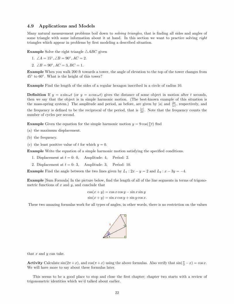
Example [Sum Formula] In the picture below, find the length of all of the line segments in terms of trigono-metric functions of x and y, and conclude that
cos(x+ y) = cosx cos y − sinx sin y
sin(x+ y) = sinx cos y + sin y cosx.
These two amazing formulas work for all types of angles, in other words, there is no restriction on the values
that x and y can take.
Activity Calculate sin(2π+x), and cos(π+x) using the above formulas. Also verify that sin(π2 −x) = cosx.We will have more to say about these formulas later.
This seems to be a good place to stop and close the first chapter; chapter two starts with a review oftrigonometric identities which we’d talked about earlier.
22

4.10 “Conditional” Identities
We’ve already learned the difference between an equation and an identity (see page 10.) Recall that the twosides of an identity are exactly the same and they differ in, perhaps, the appearance only. For convenience,we might want to switch between the two appearances; one might be simpler to use than the other in someoccasions. We start this lecture with a review of basic “identities” and then show how we should use themin solving some problems. It is important to realize that you can easily solve almost all of the problems ofthe corresponding sections by applying the following two “rules:”
1. Write the given expression in terms of sine and cosine only. (Also recall that cofunctions of comple-mentary angles are equal.)
2. Apply some algebraic massage so that you can use the Pythagorean identity sin2 t + cos2 t = 1 to“simplify.”
Note: You should take advantage of other forms of the Pythagorean identity too, eg
cos2 t = 1− sin2 t = (1− sin t)(1 + sin t) etc.
Example Suppose sin(π2 − x) = 15 and that sinx < 0. Find tanx.
Example “Simplify” the following expressions as much as you can. (In this problem you don’t need to worryabout the change in the domains of definitions as you “simplify” the expressions.)
1. (sinx+ cosx)2.
2. sin2 y1−cos y .
3. tanx+ cos x1+sin x .
4. sec4 x− tan4 x.
5. 3 cos2 t+ 3 cos2 t tan2 t.
6. tan x1+sec x + 1+sec x
tan x .
7. sin(−13◦) + cos(77◦).
Example Use the trigonometric substitution to write the algebraic equation as a trigonometric equation ofθ, where −π/2 < θ < π/2. Then find sin θ, cos θ.
1. 3 =√
9− x2, x = 3 sin θ.
2. 2√
2 =√
16− 4x2, x = 2 cos θ.
Example Verify the following (conditional) identities.
1. cos2 x− sin2 x = 2 cos2 x− 1.
2. 1cos x+1 + 1
cos x−1 = −2 cscx cotx.
3. sin2 α− sin4 α = cos2 α− cos4 α.
4. cot3 tcsc t = cos t(csc2 t− 1).
5.√
1+sin θ1−sin θ = 1+sin θ
| cos θ| .
6. tan(sin−1 x−14
)= x−1√
16−(x−1)2.
23

4.11 Solving Trigonometric Equations
Activity Discuss the number of solutions to the equation secx = c where c = .1, 5. Answer the samequestion with the restriction 0 ≤ x < 2π.
Activity Set your calculator on the radians mode and enter any number from [0, 1] into it. Then keeppressing the cosine button until the screen becomes steady. Have you got .739 . . . on your screen? Discussthe meaning of the “steady” screen and hence the source of this mysterious number.
Example Solve the following trigonometric equations.Note: The solutions of f(x) = 0 are the x− intercepts of the graph of y = f(x) in the xy-plane.
1. 2 cosx+ 1 = 0. [Isolate the trigonometric function.]
2.√
3 cscx− 2 = 0.
3. cos 5x = − 12 . [First solve cos z = − 1
2 for z and then find x using the relation z = 5x or x = z5 .]
4. sin 2x = −√32 .
5. 3 sec2 x − 4 = 0. [Isolate and take the square root to get two equations of the form secx = a andsecx = −a. Then solve each of them as in the previous problems.]
6. 2 cos2 x + cosx − 1 = 0. [First solve 2z2 + z − 1 = 0 for z and then find x by solving the obtainedequation(s) cosx = z.]
7. 2 sec2 x + tan2 x − 3 = 0. [Use an identity to write in terms of secant or tangent only, then solve asprevious problems.]
8. sin2 x = 3 cos2 x.
9. (tanx− 1) tan 3x = 0. [Recall that ab = 0 if a = 0 or b = 0.]
10. secx cscx = 2 cscx. [Factor similar terms and solve like the previous part.]
11. cosx+ 1 = sinx. [Square both sides and it becomes a quadratic equation after a suitable substitution.]
12. cscx+ cotx = 1. [It’s the previous problem in disguise.]
13. sec2 x+ 3 secx− 10 = 0. [Use inverse functions where needed.]
4.12 Sum and Difference Formulas
We’ve seen that trigonometric functions are not additive in the sense that, for instance, sin(x+ y) 6≡ sinx+sin y. Remember the sum formulas from the last example on page 15 which enable us to find exact valuesof expressions such as sin(x + y) given the value of trigonometric functions at x and y. Using the parity oftrigonometric functions, we can derive the difference formulas as well and write them together in the form:
sin(x± y) = sinx cos y ± sin y cosx
cos(x± y) = cosx cos y ∓ sinx sin y.
Now I want to digress briefly to tell you why these formulas work and where they actually come from as anamazing application of complex numbers in geometry.
Activity Remember that tangent is the quotient of sine and cosine functions by definition. Use the aboveformulas to show that
tan(x± y) =tanx± tan y
1∓ tanx tan y.
Example Write the expression as the sine, cosine, or tangent of an angle.
1. sin 3 cos 1.2− cos 3 sin 1.2.
24

2. cosπ/7 cosπ/5− sinπ/7 sinπ/5.
3. tan 2x+tan x1−tan 2x tan x .
Example Find the exact value of each expression.
1. Sine, cosine, and tangent of 15◦.
2. sin(135◦ − 30◦).
3. cos(π/4 + π/3). [Compare with cos(π/4) + cos(π/3).]
Example Find the exact value of the trigonometric function given that sinu = 513 and cos v = − 3
5 and thatu, v lie in the first and second quadrants respectively.
1. sin(u+ v).
2. sec(u+ v).
3. cot(u+ v).
4. tan(v − u).
Example Write as an algebraic expression.
1. sin(arcsinx+ arccosx).
2. cos(arccosx− arctanx).
Example Verify the following.
1. cos(5π/4− x) = −√
2/2(cosx+ sinx).
2. tan(θ + π/4) tan(θ − π/4) = −1. [What does this mean geometrically?]
3. cos(x+ y) cos(x− y) = cos2 x− sin2 y.
4. sin(x+y)−sin xh = cosx sinh
h − sinx 1−coshh .
Example Find all solutions of the given equations in the interval [0, 2π).
1. sin(x+ π)− sinx+ 1 = 0.
2. cos(x+ π/4)− cos(x− π/4) = 1.
3. sin(x+ π/2)− cos2 x = 0.
25

4.13 Multiple-Angle and Product-to-Sum Formulas
Double-Angle Formulas
sin 2x = 2 sinx cosx, cos 2x = cos2 x− sin2 x = 2 cos2 x− 1 = 1− 2 sin2 u
tan 2x =2 tanx
1− tan2 x.
Example Find the exact solutions of the equation in the interval [0, 2π).
1. sin 2x+ cosx = 0.
2. cos 2x− cosx = 0.
3. sin 4x = −2 sin 2x. [Make sure you’ve found all of the solutions in [0, 2π).]
4. tan 2x− cotx = 0.
Example Use a double-angle formula to rewrite the expression.
1. sinx cosx.
2. 4− 8 sin2 x.
Example Find the exact values of sin 2x, cos 2x, tan 2x using the double angle formulas.
1. sinx = −3/5, 3π/2 < x < 2π.
2. tanx = 3/5, 0 < x < π/2.
3. secx = −2, π/2 < x < π.
Power-Reducing Formulas
sin2 x =1− cos 2x
2, cos2 x =
1 + cos 2x
2, tan2 x =
1− cos 2x
1 + cos 2x.
Half-Angle Formulas
sinx
2= ±
√1− cosx
2
cosx
2= ±
√1 + cosx
2
tanx
2=
1− cosx
sinx=
sinx
1 + cosx.
Caution: The signs of sinx/2 and cosx/2 depend on the quadrant in which x/2 (and not x) lies.
Example Use the power-reducing formulas to rewrite the expression in terms of the first power of the cosine.
1. cos4 x.
2. sin4 x cos4 x.
3. tan4 2x.
Example Suppose sinx = −3/5 and x lies in the third quadrant. Find sin(x/2). [Ans: 3/√
10]
Example Use the half-angle formulas to determine the exact values of the sine, cosine, and tangent of theangles 75◦, and π/8.
Example Find all solutions of the equation in the interval [0, 2π).
1. sin x2 + cosx = 0.
2. tan x2 − sinx = 0.
26

Product-to-Sum Formulas
sinx sin y =1
2[cos(x− y)− cos(x+ y)]
cosx cos y =1
2[cos(x− y) + cos(x+ y)]
sinx cos y =1
2[sin(x+ y) + sin(x− y)]
Sum-to-Product Formulas
sinx+ sin y = 2 sin
(x+ y
2
)cos
(x− y
2
)sinx− sin y = 2 sin
(x− y
2
)cos
(x+ y
2
)cosx+ cos y = 2 cos
(x+ y
2
)cos
(x− y
2
)cosx− cos y = −2 sin
(x− y
2
)sin
(x+ y
2
)Example Use the product-to-sum formulas to write the product as a sum or difference.
1. 3 sinπ/3 cosπ/6.
2. cos 2t cos 4t.
3. 5 sin(−4a) sin(6a).
Example Use the sum-to-product formulas to find the exact value of the expression.
1. sin 75◦ + sin 15◦.
2. cos( 3π4 )− cos(π4 ).
Example Find all solutions of the equation in the interval [0, 2π).
1. sin 6x+ sin 2x = 0.
2. cos 2xsin 3x−sin x − 1 = 0.
Example Verify the given “identities.”
1. 1 + cos 10y = 2 cos2 5y.
2. tan(u/2) = cscu− cotu.
3. cos 4x+cos 2xsin 4x+sin 2x = cot 3x.
27
4.14 Law of Sines
In 13th century, Tusi, an Iranian mathematician and astronomer, formulated the law of sines for plane tri-angles which we will now describe.
Law of Sinesa
sinA=
b
sinB=
c
sinC,
where a, b, and c are the lengths of the sides of a triangle, and A,B, and C are the opposite angles.Remark: In the above relation, the common value of the three fractions is actually the diameter of thetriangle’s circumcircle.
The law of sines can be used to compute the remaining sides of a triangle when two angles and a side areknown (AAS or ASA). It can also be used when two sides and one of the non-enclosed angles are known (SSA).In some such cases, the formula gives two possible values for the enclosed angle, leading to an ambiguous case.
Example Solve (if possible) the triangle(s) 4ABC assuming ∠B = 45◦,∠C = 105◦, b = 20. [Ans:A = 30◦, a ≈ 14.1, c ≈ 27.3]
Example A tree is leaning 4◦ from the vertical. At a point 40 meters from the tree, the angle of elevationis 30◦ degrees. Find the height of the tree. [Ans: 24.1 m]
Example Solve (if possible) the triangle(s) 4ABC assuming ∠A = 110◦, a = 125, b = 100. [sin 110◦ ≈ .9]
Activity Suppose b = 200 and try to solve the previous problem again.
Example [The Ambiguous Case] Solve (if possible) the triangle(s)4ABC assuming ∠A = 45◦, b =√62 , a = 1.
4.15 Law of Cosines
In physics one frequently needs to find the net “force” exerted on a body. This often leads to solving atriangle given two sides and and their included angle (SAS). The common method to solve a triangle in cases(SAS) and also (SSS) is by means of a formula discovered in its modern form by Kashani, a great Iranianmathematician and astronomer of 14th century, usually known as law of cosines.
Law of Cosinesa2 = b2 + c2 − 2bc cosA
where a, b, and c are the lengths of the sides of a triangle, and A,B, and C are the opposite angles.
Activity Discuss how the law of cosines generalizes the Pythagorean identity.
Example Solve the triangle 4ABC if
1. ∠A = 30◦, b = 1, c = 2.
2. a = 7, b = 3, c = 8. [Ans: A ≈ 60◦, B ≈ 21.8◦, C ≈ 98.2◦]
4.16 Area Formulas
Recall that the area of a triangle is one-half the product of a height and its associated base. In cases wherewe don’t have the length of the height at hand we can use one of the following two formulas.
• Area = 12ab sinC.
• Heron’s formula named after Heron of Alexandria:
Area =√s(s− a)(s− b)(s− c),
where s is the semiperimeter of the triangle: s = a+b+c2 .
28

The student should notice that Heron’s formula is depends only on the sides of the triangle as the sidesuniquely determine the triangle and hence the angles. Similar area formulas for quadrilaterals (eg that ofBrahmagupta) cannot be entirely in terms of the sides.Example Find the area of the triangle 4ABC if ∠A = 30◦, b = 2, c = 4.
Example Find the area of 4ABC with a = 3, b = 4, c = 5 using the three formulas above.
29