the stochastic actor-oriented model network...
TRANSCRIPT

Network Modeling
Viviana Amati Jurgen Lerner David Schoch
Dept. Computer & Information ScienceUniversity of Konstanz
Winter 2013/2014(version 05 February 2014)
Outline
IntroductionWhere are we going?
The Stochastic actor-oriented modelData and model definitionModel specificationParameter interpretationSimulating network evolutionParameter estimation: MoM and MLE
Extending the model: analyzing the co-evolution of networks and behaviorMotivationSelection and influenceModel definition and specificationSimulating the co-evolution of networks and behaviorParameter interpretationParameter estimation
Something more on the SAOM
ERGMs and SAOMs
Outline
IntroductionWhere are we going?
The Stochastic actor-oriented model
Extending the model: analyzing the co-evolution of networks and behavior
Something more on the SAOM
ERGMs and SAOMs
Where we are
Model Main feature Real dataG(n,p) ties are independent ties dependency
Planted partition intra/inter group density ties dependency
Preferential attachment degree distribution other structural properties
ERGM class of models reasonable representation
These are models for cross-sectional data

Where we are going
Network are dynamic by nature. How to model network evolution?
We need a model for longitudinal data
Networks are dynamic by nature: a real example
The Teenage Friends and Lifestyle Study analyzes smoking behavior andfriendship
Data collection: (available from http://www.stats.ox.ac.uk/∼snijders/siena/)
- One school year group monitored over 3 years;
- questionnaires at approximately one year interval:
1. Friendship relation: each pupil could name up to 12 friends2. Individual information and lifestyle elements: gender, age,
substances use, smoking of parents and siblings etc.
arrows = friendship relationgender: circle = girl, square = boysmoking behavior: blue = non, gray = occasional, black = regular
Networks are dynamic by nature: a real example Networks are dynamic by nature: a real example

Networks are dynamic by nature: a real example Some questions
Is there any tendency in friendship formation ...
- towards reciprocity?
- towards transitivity?
Some questions
Is there any homophily in friendship formation with respect to ...
- gender?
- smoking behavior?
Solution
Stochastic actor-oriented model (SAOM)
Aim
Explain network evolution as a result of
- endogenous variables: structural effects depending on the network only(e.g. reciprocity, transitivity, etc.)
- exogenous variables: actor-dependent and dyadic-dependent covariates(e.g. effect of a covariate on the existence of a tie or on homophily)
simultaneously

Background: random variables
Definitions
Let (Ω,P) be a probability space
Ω = is a set of possible outcomes
P : Ω→ [0,1] is a probability functionsuch that:
1. P(ω)≥ 02.∑ω∈Ω
P(ω) = 1
1. P((a,b)) =1
36, a,b ∈ 1,2, · · · ,6
2.∑ω∈Ω
P(ω) = 1
A (real-valued) random variable (r.v.) is a function X : (Ω,P)→ (R,P).
Background: random variables (motivation)
Example
Background: random variables (motivation)
Example
Given P(ω) we can compute P(x):
P(X = 4) = P((1,3)) + P((2,2)) + P((3,1)) = 1/36 + 1/36 + 1/36 = 1/12
Background: random variables (motivation)
Example
N.b.:- capital letters denote r.vs (e.g. X=sum of two dice)- small letters denote the values assumed by a r.v. (e.g. x=2)- The set of values that X can take is called range and will be denoted by S(e.g. S = 2,3, . . . ,12 )

Background: discrete random variable
DefinitionA r.v. X is defined to be discrete if S is countable.
The probability mass function (p.m.f) ϕX (x) : R→ [0,1] describes the valuesthat X can take along with the probability associated with each value
x ϕX (x)2 1/363 2/364 3/365 4/366 5/367 6/368 5/369 4/36
10 3/3611 2/3612 1/36
Background: discrete random variable
DefinitionA r.v. X is defined to be discrete if S is countable.
The probability mass function (p.m.f) ϕX (x) : R→ [0,1] describes the valuesthat a X can take along with the probability associated with each value
ϕX (x) = P(X = x)
The cumulative distribution function (c.d.f.) FX (x) : R→ [0,1] describes theprobability that X takes value lower than x
FX (x) = P(X ≤ x) =∑x ′<x
P(X = x ′)
ExamplesX=Sum of two dice
P(X ≤ 3) = P(X = 2) + P(X = 3) = 1/36 + 2/36 = 1/12
Background: continuous random variable
DefinitionA random variable X is called (absolutely) continuous if S is uncountable andthere exists a function fX (x) : R→ R+ such that
FX (x) = P(X ≤ x) =
∫ x
−∞fX (u)du ∀x ∈ R
P(X ∈ R) =
∫ +∞
−∞fX (x)dx = 1
fX (x) is the probability density function (p.d.f)
Examples
- X = weight of people in a population- X = waiting time at a post office clerk- . . .
Background: continuous random variable
The p.d.f. fX (x) allows to compute all the probability statements about X . Forinstance, the probability that X takes values in [a,b] is
P(a ≤ X ≤ b) =
∫ b
afX (x)dx
Geometrical interpretation
Intuition suggests that
P(X = x) =
∫ x
xfX (u)du = 0
Thus, we cannot determinea continuous random vari-able via its “mass function”

Background: stochastic (or random) process
DefinitionA stochastic process X(t), t ∈ T is a mapping
∀t ∈ T 7→ X(t) : Ω→ R
Background: stochastic process
T = index set (usually interpreted as time)S = state space
Different stochastic processes can be defined according to S and T
S T
Countable (discrete) Uncountable (continuous)
Countable discrete-time with continuous-time with(finite) finite state space finite state space
Uncountable discrete-time with continuous-time with(continuous) continuous state space continuous state space
Background: stochastic process
ExampleX(t) = the outcome of flipping a coin
S = −1,1, where −1 =tail 1 =headT = 1,2, · · ·
X(t), t ∈ T is a discrete-time stochastic process with a finite state space
Background: stochastic process
ExampleX(t) = the number of telephone call at a switchboard of a company
from 8 a.m. to 8 p.m.
S = 0,1,2, · · ·T = [0,12]
X(t), t ∈ T is a continuous-time stochastic process with a finite state space

Background: continuous-time Markov Chain
DefinitionX(t), t ∈ T has the Markov property if:
∀ x ∈ S and ∀ ti < tj
P(X(tj ) = x(tj ) | X(t) = x(t) ∀ t ≤ ti ) = P(X(tj ) = x(tj ) | X(ti ) = x(ti ))
DefinitionA continuous-time Markov chain Xt , t ≥ 0 is a stochastic process having
1. finite state2. continuous-time3. the Markovian property
Background: continuous-time Markov Chain
ExampleX(t) = # of goals that a given soccer player scores by time t (time played
in official matches)
X(t), t ≥ 0 is a continuous-time Markov chains
Why?
1. state space: S = 0,1,2, . . . ,BB = total number of goals scored during the career
2. the time is continuous: [0,T]T = time of retirement
3. the process X(t), t ≥ 0 has the Markov property
Background: Markov property Background: describing a continuous-time Markov chain

Background: describing a continuous-time Markov chain
Holding timeT = amount of time the chain spends in state i (Exponential r.v.)
fT (t) = λi e−λi t , λi > 0, t > 0
fT (t) : R+→ R+ such that
P(T ≤ t′) =
∫ t′
0fT (t)dt = 1− e−λi t′ ∀t ≥ 0
Background: describing a continuous-time Markov chainHolding timeT = amount of time the chain spends in state i (Exponential r.v.)
fT (t) = λi e−λi t , λi > 0, t > 0
λi is the rate parameter
The Exponential r.v. has the memoryless property
P(T > s + t | T > t) = P(T > s) ∀ s, t > 0
Background: describing a continuous-time Markov chain Background: describing a continuous-time Markov chain
Jump chain
P = (pij : i , j ∈ S) = jump matrix
pij = P(X(t′) = j|X(t) = i , the opportunity to leave i)
pij ≥ 0∑j∈S
pij = 1 ∀i , j ∈ S

Background: describing a continuous-time Markov chain
Example
P =
0.1 0 0.6 0.30.8 0.1 0.1 0
0.05 0.5 0.05 0.40.6 0.1 0.15 0.15
Outline
Introduction
The Stochastic actor-oriented modelData and model definitionModel specificationParameter interpretationSimulating network evolutionParameter estimation: MoM and MLE
Extending the model: analyzing the co-evolution of networks and behavior
Something more on the SAOM
ERGMs and SAOMs
Recall: adjacency matrix and directed relations
Social network: a set of actors N + a relation R
Graph = G(N,R) Adjacency matrix=X
- 0 0 0 01 - 1 0 00 0 - 0 00 1 1 - 01 1 0 0 -
Directed relation:
6=⇒i → j j → i
Data
Longitudinal (or panel) network data = M (≥ 2) repeated observations on anetwork
x(t0), x(t1), . . . , x(tm), . . . , x(tM−1), x(tM)
- set of actors N = 1,2, . . . ,n- a non reflexive and directed relation R
- actor covariates V (gender, age,social status, ...)

Model definition: assumptions
Network evolution is the outcome of a stochastic process specified by thefollowing assumptions:
1. Ties are state:a tie is a state with a tendency to endure over time
2. Distribution of the process:X(t), t ∈ T is a continuous time Markov Chain defined on:
- the state space X
- the set of actors N
Model definition: assumptionsFinite state space: X is the set of all possible adjacency matrices defined on N
X = 2n(n−1)⇒X is a countable set
Model definition: assumptions
Continuous-time process
Latent process: the network evolves in continuous-time butwe observed it only at discrete time points
Model definition: assumptions
Markov property: the current state of the network determines probabilisticallyits further evolution

Model definition: assumptions3. Opportunity to change: at any given moment t one actor has the
opportunity to change
Model definition: assumptions3. Opportunity to change: at any given moment t one actor has the
opportunity to change
Model definition: assumptions4. Absence of co-occurrence: no more than one tie can change at any given
moment t(Notation: x(i ; j) means that actor i changes his outgoing tie towards j)
Model definition: assumptions
5. Actor-oriented perspective: actors control their outgoing ties
- change in ties are made by the actor who sends the ties
- decisions are made according to the position of the actor in thenetwork, his attributes and the characteristics of the others
Aim: maximize a utility function
- actors have complete knowledge about the network and all the otheractors
- the maximization is based on immediate returns (myopic actors)

Model definition: assumptions (recap)
1. Ties are states
2. The evolution process is a continuous-time Markov chain
3. At any given moment t one probabilistically selected actor has theopportunity to change
4. No more than one tie can change at any given moment t
5. Actor-oriented perspective
Model definition
Consequences of the assumptions
The evolution process can be decomposed into micro-steps
Micro-step Continuous-time Markov chain- the time at which i had - the waiting time until the next opportunitythe opportunity to change for a change made by an actor i
(holding time)
- the precise change i made - the probability of changing the link xijgiven that i is allowed to change(jump chain)
Distribution of the holding time: rate function
Transition matrix of the jump chain: objective function
Model definition: rate function
How fast is the opportunity for changing?
Waiting time between opportunities of change for actor i ∼ Exp (λi )
λi is called the rate function
Simple specification: all actors have the same rate of change λ
P(i has the opportunity of change) =1n ∀i ∈N
Model definition: rate function
How fast is the opportunity for changing?
More complex specification
Actors may change their ties at different frequencies λi (α,x ,v)
Example“Young girls might change their ties more frequently”
λi (α,x ,v) = αage ∗ vage +αgender ∗ vgender
It follows
P(i has the opportunity of change) =λi (α,x ,v)
n∑j=1
λj (α,x ,v)

Model definition: rate function
How fast is the opportunity for changing?
In the following we assume that:
- all actors have the same rate of change
=⇒ λ is constant over the actors
- the frequencies at which actors have the opportunity to make a changedepends on time
=⇒ λ is not constant over time
As a consequence, we must specify M−1 rate functions
λ1, · · · , λM−1
Model definition: objective function
Which tie is changed?
Changing a tie means turning it into its opposite:
xij = 0 is changed into xij = 1 tie creation
xij = 1 is changed into xij = 0 tie deletion
Given that i has the opportunity to change:
Possible choices of i Possible reachable statesn−1 changes n−1 networks x(i ; j)
1 non-change 1 network equal to x
Model definition: objective function Model definition: objective function

Background: random utility model
Setting:decision makers who face a choice between N-alternatives
Notation:i denotes the decision makerJ = 1, . . . , j, . . . ,N choice setJ is exhaustive and choices are mutually exclusive
Assumption:the decision makers obtain a certain level of profit from each alternative.The profit is modeled by the utility function Uij : J → R
Decision rule: i chooses the alternative j that assures him the highest profit, i.e.
j : maxj∈J Uij
Background: random utility model
The researcher does not observe the decision maker’s utility, but only:- n×A matrix x of attributes of each alternative j (as faced by i)- B×1 vector vi of attributes of i
Since, there are factors that the researcher cannot observe, the utility functionis decomposed as
Uij = Fij (β,γ,xij ,vi ) +Eij
where:- Fij is the deterministic part of the utility (observed!)
Fij (β,γ,xij ,vi ) =∑
aβaxija +
∑b=1
γbvib , βa, γb ∈ R,xij
- Eij : random term (not observed!)The random term are independent and identically distributed.
Consequence: The researcher can only “guess” i ’s choice
Background: random utility modelDecision probabilities:it is assumed that Eij is Gumbel distributed
fEij (ε) = e−εe−e−ε ε ∈ R
so that the probability that i chooses the alternative j is given by
pij = P(Uij > Uih, ∀ h ∈ J) =eFij
N∑h=1
eFih
Model definition: objective function
Actors change their ties in order to maximize a utility function
ui (β,x(i ; j)) = fi (β,x(i ; j),vi ,vj ) +Eij
- fi (β,x(i ; j),vi ,vj ) is the objective function- Eij is assumed to be distributed as a Gumbel r.v.
Consequence: the probability that i changes his outgoing tie towards j is:
pij =exp(
fi (β,x(i ; j),vi ,vj )))
n∑h=1
exp(
fi (β,x(i ; h),vi ,vj ))
Probabilities interpretation:pij is the probability that i changes the tie towards jpii is the probability of not changing
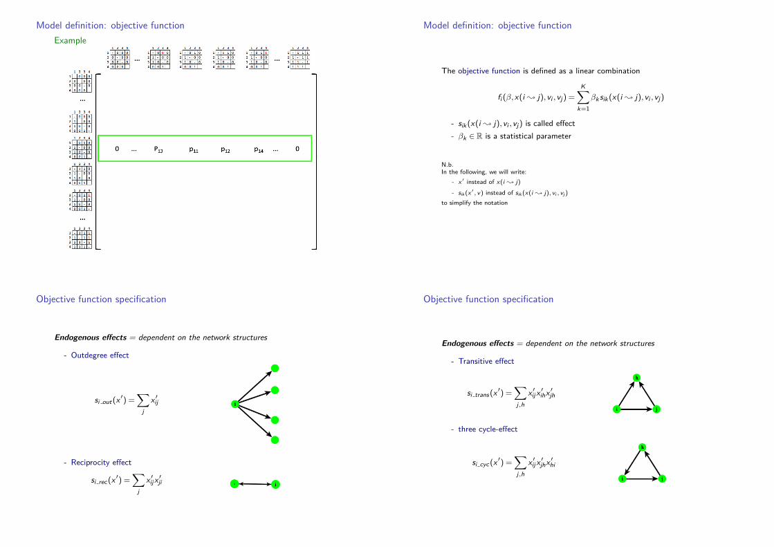
Model definition: objective functionExample
Model definition: objective function
The objective function is defined as a linear combination
fi (β,x(i ; j),vi ,vj ) =
K∑k=1
βk sik (x(i ; j),vi ,vj )
- sik (x(i ; j),vi ,vj ) is called effect- βk ∈ R is a statistical parameter
N.b.In the following, we will write:
- x ′ instead of x(i ; j)- sik (x ′,v) instead of sik (x(i ; j),vi ,vj )
to simplify the notation
Objective function specification
Endogenous effects = dependent on the network structures
- Outdegree effect
si out (x ′) =∑
jx ′ij
- Reciprocity effect
si rec (x ′) =∑
jx ′ij x ′ji
Objective function specification
Endogenous effects = dependent on the network structures
- Transitive effect
si trans (x ′) =∑j,h
x ′ij x ′ihx ′jh
- three cycle-effect
si cyc (x ′) =∑j,h
x ′ij x ′jhx ′hi

Objective function specification
Exogenous effects = related to actor’s attributes
Example
- Friendship among pupils:Smoking: non, occasional, regular
Gender: boys, girls
- Trade/Trust (Alliances) among countries:Geographical area: Europe, Asia, North-America,...
Worlds: First, Second, Third, Fourth
Objective function specification
Exogenous effects (individual covariate)- covariate-ego
si cego(x ′,v) =∑
jx ′ij vi
- covariate-alter
si calt (x ′,v) =∑
jx ′ij vj
Objective function specification
Exogenous effects (dyadic covariate)- covariate-related similarity
si csim(x ′,v) =∑
jx ′ij
(1−
∣∣vi − vj∣∣
RV
)
where RV is the range of V and(
1− |vi−vj |RV
)is called similarity score
Remark:
when V is a binary covariate, the covariate-related similarity can be written inthe following way:
si csim(x ′,v) =∑
jx ′ij I
vi = vj
Objective function specification
Which effects must be included in the objective function?
Outdegree and Reciprocity must always be included.The choice of the other effects must be determined according tohypotheses derived from theory
ExampleFriendship network
Theory Effectthe friend of my friend ⇒ transitive effectis also my friendgirls trust girls ⇒ covariate-relatedboys trust boys similarity

Parameter interpretation
1. Parameter interpretation: βk quantifies the role of sik (x ′) in the networkevolution.
- βk = 0: sik (x ′) plays no role in the network dynamics
- βk > 0: higher probability of moving into networks where sik (x ′) is higher
- βk < 0: higher probability of moving into networks where sik (x ′) is lower
2. The preferences driving the choice of the actors have the same intensitiesover time
=⇒ β1, · · · ,βK are constant over time
Parameter interpretation
The procedures for estimating the parameters of the SAOM are implementedin a R library called RSiena
(SIENA = Simulation Investigation for Empirical Network Analysis)
The R script “estimation.R” contains the R commands to implement theestimation procedure in R and the folder “tfls.zip” includes the data files.
Example data: an excerpt from the “Teenage Friends and Lifestyle Study” dataset:
- Networks: relation = friendshipNetworks: actors = 129 pupils present at all three measurement points
- Covariates: gender (1 = Male, 2 = Female)Covariates: smoking behavior (1 = no, 2= occasional, 3 = regular)
Parameter interpretation: a very simple model
Estimates s.e. t-scoreRate parameters:Rate parameter period 1 8.5948 ( 0.7091 )Rate parameter period 2 7.2115 ( 0.5751 )
Other parameters:outdegree (density) -2.4147 ( 0.0387 ) -62.3875reciprocity 2.7106 ( 0.0811 ) 33.4061
Rate parameter: expected frequency, between two consecutive networkobservations, with which actors get the opportunity to change a network tie
- about 9 opportunities for change in the first period- about 7 opportunities for change in the second period
The estimated rate parameters will be higher than the observed number ofchanges per actor (why?)

Parameter interpretation: a very simple model
Interpreting the objective function parameters:
The parameter βk quantifies the role of the effect sik in the network evolution.
βk = 0 sik plays no role in the network dynamics
βk > 0 higher probability of moving into networks where sik is higher
βk < 0 higher probability of moving into networks where sik is lower
Which βk are “significantly” different from 0?
E.g. βrec = 0.13 is “significantly” different from 0?
Parameter interpretation: a very simple model
Hypothesis test:
1. State the hypotheses.- The null hypothesis (H0):
the observed increase or decrease in the number of networkconfigurations related to a certain effect results purely from chance
H0 : βk = 0
- The alternative hypothesis (H1):the observed increase or decrease in the number of networkconfigurations related to a certain effect is influenced by somenon-random cause.
H1 : βk 6= 0
Parameter interpretation: a very simple modelHypothesis test:
2. Define a decision rule∣∣∣ βk
s.e.(βk )
∣∣∣≥ 2 reject H0∣∣∣ βks.e.(βk )
∣∣∣< 2 fail to reject H0
2 · s.e.(βk ) 2 · s.e.(βk )
H0 : βk = 0
Parameter interpretation: a very simple model
Estimates s.e. t-scoreRate parameters:Rate parameter period 1 8.5948 ( 0.7091 )Rate parameter period 2 7.2115 ( 0.5751 )
Other parameters:outdegree (density) -2.4147 ( 0.0387 ) -62.3875reciprocity 2.7106 ( 0.0811 ) 33.4061
Objective function parameters:- outdegree parameter: the observed networks have low density- reciprocity parameter: strong tendency towards reciprocated ties
Parameter interpretation: a very simple model
In more detail
βout
n∑j=1
x ′ij +βrec
n∑j=1
x ′ij x ′ji =−2.4147n∑
j=1x ′ij + 2.7106
n∑j=1
x ′ij x ′ji
Adding a reciprocated tie (i.e., for which xji = 1) gives
−2.4147 + 2.7106 = 0.2959
while adding a non-reciprocated tie (i.e., for which xji = 0) gives
−2.4147
Conclusion: reciprocated ties are valued positively and non-reciprocated ties arevalued negatively by actors
Parameter interpretation: a more complex model
Specifying the objective function
In friendship context, sociological theory suggests that:- friendship relations tend to be reciprocated → reciprocity effect
- the statement “the friend of my friend is also my friend” is almost alwaystrue → transitive triplets effect
Parameter interpretation: a more complex model
Specifying the objective function
In friendship context, sociological theory suggests that:- pupils prefer to establish friendship relations with others that are similar to
themselves → covariate similarity
This effect must be controlled for the sender and receiver effects of thecovariate.
- Covariate ego effect
- Covariate alter effect

Parameter interpretation: a more complex model
Estimates s.e. t-scoreRate parameters:Rate parameter period 1 10.6809 ( 1.0425 )Rate parameter period 2 9.0116 ( 0.8386 )
Other parameters:outdegree (density) -2.8597 ( 0.0608 ) -47.0288reciprocity 1.9855 ( 0.0876 ) 22.6765transitive triplets 0.4480 ( 0.0257 ) 17.4558sex alter -0.1513 ( 0.0980 ) -1.5445sex ego 0.1571 ( 0.1072 ) 1.4659sex similarity 0.9191 ( 0.1076 ) 8.5440smoke alter 0.1055 ( 0.0577 ) 1.8272smoke ego 0.0714 ( 0.0623 ) 1.1469smoke similarity 0.3724 ( 0.1177 ) 3.1647
- outdegree parameter: the observed networks have low density- reciprocity parameter: strong tendency towards reciprocated ties- transitivity parameter: preference for being friends with friends’friends
Parameter interpretation: a more complex model
Estimates s.e. t-scoreRate parameters:Rate parameter period 1 10.6809 ( 1.0425 )Rate parameter period 2 9.0116 ( 0.8386 )
Other parameters:outdegree (density) -2.8597 ( 0.0608 ) -47.0288reciprocity 1.9855 ( 0.0876 ) 22.6765transitive triplets 0.4480 ( 0.0257 ) 17.4558sex alter -0.1513 ( 0.0980 ) -1.5445sex ego 0.1571 ( 0.1072 ) 1.4659sex similarity 0.9191 ( 0.1076 ) 8.5440smoke alter 0.1055 ( 0.0577 ) 1.8272smoke ego 0.0714 ( 0.0623 ) 1.1469smoke similarity 0.3724 ( 0.1177 ) 3.1647
- sex alter: gender does not affect actor popularity- sex ego: gender does not affect actor activity- sex similarity: tendency to choose friends with the same gender
Parameter interpretation: a more complex model
- Gender: coded with 1 for boys and with 2 for girls.
- All actor covariates are centered: v = 1.434 is the mean of the covariate
vi − v =
−0.434 for boys
0.566 for girls
- The contribution of xij to the objective function is
βego(vi − v) +βalter (vj − v) +βsame(Ivi = vj− simv
)=
= 0.1571(vi − v)−0.1513(vj − v) + 0.9191(Ivi = vj−0.5048
)where simv is the average of the similarity score.
Parameter interpretation: a more complex model
Male FemaleMale 0.4526 -0.618Female -0.309 0.4584
Table : Gender-related contributions to the objective function
Conclusions: Preference for intra-gender relationships.

Parameter interpretation: a more complex model
Estimates s.e. t-scoreRate parameters:Rate parameter period 1 10.6809 ( 1.0425 )Rate parameter period 2 9.0116 ( 0.8386 )
Other parameters:outdegree (density) -2.8597 ( 0.0608 ) -47.0288reciprocity 1.9855 ( 0.0876 ) 22.6765transitive triplets 0.4480 ( 0.0257 ) 17.4558sex alter -0.1513 ( 0.0980 ) -1.5445sex ego 0.1571 ( 0.1072 ) 1.4659sex similarity 0.9191 ( 0.1076 ) 8.5440smoke alter 0.1055 ( 0.0577 ) 1.8272smoke ego 0.0714 ( 0.0623 ) 1.1469smoke similarity 0.3724 ( 0.1177 ) 3.1647
- smoke alter: smoking behavior does not affect actor popularity- smoke ego: smoking behavior not affect actor activity- smoke similarity: tendency to choose friends with the same smoking
behavior
Parameter interpretation: a more complex model
- Smoking behavior: coded with 1 for “no”, 2 for “occasional”, and 3 for“regular” smokers.
- The smoking covariate is centered: v = 1.310 is the mean of the covariate
vi − v =
−0.310 for no smokers
0.690 for occasional smokers
1.690 for regular smokers
- The contribution of xij to the objective function is
βego(vi − v) +βalter (vj − v) +βsame(
1− |vi−vj |Rv− simv
)=
= 0.0714(vi − v) + 0.1055(vj − v) + 0.3724(
1− |vi−vj |2 −0.7415
)
Parameter interpretation: a more complex model
no occasional regularno 0.0414 -0.0734 -0.1882occasional -0.0393 0.2183 0.1035regular -0.1200 0.1376 0.3952
Table : Smoking-related contributions to the objective function
Conclusions:- preference for similar alters- this tendency is strongest for high values on smoking behavior
Simulating network evolution
Aim: given x(t0) and fixed parameter values, provide x sim(t1)according to the process behind the SAOM
⇓
reproduce a possible series of micro-steps between t0 and t1
Input
n = number of actorsλ = rate parameter (given)β = (β1, . . . ,βk ) = objective function parameters (given)x(t0) = network at time t0 (given)
Output
x sim(t1) = network at time t1

Simulating network evolution
Algorithm 1: Network evolutionInput: x(t0), λ, β, nOutput: x sim(t1)t← 0x ← x(t0)while condition = TRUE do
dt ∼ Exp(nλ)i ∼ Uniform(1, . . . ,n)j ∼ Multinomial(pi1, . . . ,pin)if i 6= j then
x ← x(i ; j)else
x ← xt← t + dt
x sim(t1)← xreturn x sim(t1)
t = timedt = holding time between consecutive opportu-nities to change∼ = generated from
bla blabla bla
n = 4
λ= 1.5
β = (βout ,βrec ,βtrans )βi=(-1,0.5,-0.25)
Simulating network evolution
Algorithm 1: Network evolutionInput: x(t0), λ, β, nOutput: x sim(t1)t← 0x ← x(t0)while condition = TRUE do
dt ∼ Exp(nλ)i ∼ Uniform(1, . . . ,n)j ∼ Multinomial(pi1, . . . ,pin)if i 6= j then
x ← x(i ; j)else
x ← xt← t + dt
x sim(t1)← xreturn x sim(t1)
t = timedt = holding time between consecutive opportu-nities to change∼ = generated from
bla blabla bla
Generate the time elapsedbetween t0 and the first op-portunity to change
The more intuitive way to generatedt is:
- generate the waiting time foreach actor i
wi ∼ Exp(λ)
- dt = min1≤i≤n
wi
but this requires the generation ofn numbers.
Simulating network evolution
Algorithm 1: Network evolutionInput: x(t0), λ, β, nOutput: x sim(t1)t← 0x ← x(t0)while condition = TRUE do
dt ∼ Exp(nλ)i ∼ Uniform(1, . . . ,n)j ∼ Multinomial(pi1, . . . ,pin)if i 6= j then
x ← x(i ; j)else
x ← xt← t + dt
x sim(t1)← xreturn x sim(t1)
t = timedt = holding time between consecutive opportu-nities to change∼ = generated from
blablablabla
Generate the time elapsed be-tween t0 and the first opportu-nity to change
To avoid the generation of n numbers,we use the following result:If
Wi ∼ Exp(λi ), 1≤ i ≤ n
and W1, . . . ,Wn are mutually indepen-dent, then
DT = minW1, . . . ,Wn ∼ Exp(n∑
i=1
λi )
e.g. dt = 0.0027
Simulating network evolution
Algorithm 1: Network evolutionInput: x(t0), λ, β, nOutput: x sim(t1)t← 0x ← x(t0)while condition = TRUE do
dt ∼ Exp(nλ)i ∼ Uniform(1, . . . ,n)j ∼ Multinomial(pi1, . . . ,pin)if i 6= j then
x ← x(i ; j)else
x ← xt← t + dt
x sim(t1)← xreturn x sim(t1)
t = timedt = holding time between consecutive opportu-nities to change∼ = generated from
blablablabla
Select the actor i who has theopportunity to change
e.g. i = 1

Simulating network evolution
Algorithm 1: Network evolutionInput: x(t0), λ, β, nOutput: x sim(t1)t← 0x ← x(t0)while condition = TRUE do
dt ∼ Exp(nλ)i ∼ Uniform(1, . . . ,n)j ∼ Multinomial(pi1, . . . ,pin)if i 6= j then
x ← x(i ; j)else
x ← xt← t + dt
x sim(t1)← xreturn x sim(t1)
t = timedt = holding time between consecutive opportu-nities to change∼ = generated from
blablablabla
Select j, the actor towards i isgoing to change his outgoing tie
i → j fi pij
1 → 1 -1.75 0.151 → 2 -1.00 0.311 → 3 -3.25 0.031 → 4 -0.5 0.51
Simulating network evolution
Algorithm 1: Network evolutionInput: x(t0), λ, β, nOutput: x sim(t1)t← 0x ← x(t0)while condition = TRUE do
dt ∼ Exp(nλ)i ∼ Uniform(1, . . . ,n)j ∼ Multinomial(pi1, . . . ,pin)if i 6= j then
x ← x(i ; j)else
x ← xt← t + dt
x sim(t1)← xreturn x sim(t1)
t = timedt = holding time between consecutive opportu-nities to change∼ = generated from
blablablabla
e.g. j = 4
x(1 ; 4)
Simulating network evolution
Algorithm 1: Network evolutionInput: x(t0), λ, β, nOutput: x sim(t1)t← 0x ← x(t0)while condition = TRUE do
dt ∼ Exp(nλ)i ∼ Uniform(1, . . . ,n)j ∼ Multinomial(pi1, . . . ,pin)if i 6= j then
x ← x(i ; j)else
x ← xt← t + dt
x sim(t1)← xreturn x sim(t1)
t = timedt = holding time between consecutive opportu-nities to change∼ = generated from
blablablabla
e.g. j = 1
x(1 ; 1)
Simulating network evolution
Algorithm 1: Network evolutionInput: x(t0), λ, β, nOutput: x sim(t1)t← 0x ← x(t0)while condition = TRUE do
dt ∼ Exp(nλ)i ∼ Uniform(1, . . . ,n)j ∼ Multinomial(pi1, . . . ,pin)if i 6= j then
x ← x(i ; j)else
x ← xt← t + dt
x sim(t1)← xreturn x sim(t1)
t = timedt = holding time between consecutive opportu-nities to change∼ = generated from
blablablabla
e.g. t = 0 + 0.0027

Simulating network evolution
Two different stopping rules:
1. Unconditional simulation:the simulation of the network evolution carries on until a predeterminedtime length has elapsed (usually until t = 1).
2. Conditional simulation on the observed number of changes:Simulation runs on until
n∑i,j=1ı 6=j
∣∣∣xobsij (t1)− xij (t0)
∣∣∣=
n∑i,j=1ı 6=j
∣∣∣x simij (t1)− xij (t0)
∣∣∣This criterion can be generalized conditioning on any other explanatoryvariable.
Simulating network evolution
Use of simulations:
- simulating the network evolution between two consecutive time points
N.b.For simulations of 3 or more waves (M ≥ 2), the simulations for wave m + 1 startat the simulated network for wave m.
- provide possible scenarios of the network evolution according to different valuesof the parameters of the SAOM
- estimate the parameters of the SAOM
- evaluate the goodness of fit of the model
Estimating the parameter of the SAOM
Problem
Given the longitudinal network data
x(t0), x(t1), . . . , x(tM)
and a parametrization of the SAOM
θ = (λ1, . . . ,λM ,β1, . . . ,βK )
we want to estimate θ in a plausible way.
Solution
Different estimation methods are available:
1. Method of Moments (MoM)2. Maximum Likelihood Estimation (MLE)
Background: Method of Moments (MoM)DefinitionLet X be a random variable with probability distribution depending on aparameter θ.Let (x1, . . . , xq) a sample of q observations from the r.v. X .
The expected value (mean or moment) of X , denoted by Eθ[X ], is definedby:
Eθ[X ] =∑x∈S
x ·ϕ(x ,θ)
if X is discrete with p.m.f ϕ(x ,θ) and
Eθ[X ] =
∫x∈S
x · f (x ,θ)dx
if X is continuous with p.d.f f (x ,θ)
The sample counterpart of Eθ[X ], denoted by µ, is defined by:
µ=1q
q∑i=1
xi

Background: Method of Moments (MoM)
DefinitionThe method of moment estimator for θ is found by equating the expectedvalue Eθ[X ] to its sample counterpart µ
Eθ[X ] = µ
and solving the resulting equation for the unknown parameter.The estimate for θ is denoted by θ.
In practice:1. Compute the expected value Eθ[X ]
2. Compute the sample counterpart µ= 1q
q∑i=1
xi
3. Solve the moment equation Eθ[X ] = µ for θ
MotivationOne can observe that the expected value of a certain distribution usuallydepends on the parameter θ
Background: Method of Moments (MoM)
ExampleLet W be the r.v. describing the waiting times between two consecutiveopportunities for change for an actor in a network evolution processdescribed by the SAOM.A sample is reported in the following table:
1 2 3 4 5 6 7 8 9 10wi 0.33 0.08 0.06 0.01 0.04 0.11 0.03 0.18 0.02 0.07
Estimate the rate parameter λ according to the MoM.
From the assumptions of the SAOM follows that W ∼ Exp(λ)
fW (w) = λe−λw λ,w > 0
Background: Method of Moments (MoM)
Example1. The expected value of W is:
Eλ[W ] =
+∞∫0
w · fW (w)dw =
+∞∫0
w ·λe−λw dw
=[−w · e−λw
]+∞
0−
+∞∫0
−e−λw dw
︸ ︷︷ ︸integration by parts
= 0−[− 1λ
e−λw]+∞
0=
1λ
Background: Method of Moments (MoM)
Example
1 2 3 4 5 6 7 8 9 10wi 0.33 0.08 0.06 0.01 0.04 0.11 0.03 0.18 0.02 0.07
2. The sample counterpart is:
µ=1
10
10∑i=1
wi =0.9310 = 0.093
3. The estimate for λ is the solution of:
Eλ[W ] = µ
1λ
= µ
namelyλ=
1µ
=1
0.093 = 10.75

Background: Generalizations of MoM
The principle of the MoM can be easily generalized to any function s : S 7−→ R.1. Expected value of s(X):
Eθ[s(X)] =∑x∈S
s(x)ϕ(x ,θ)
Eθ[s(X)] =
∫x∈S
s(x)f (x ,θ)dx
2. Corresponding sample moment:
γ =1q
q∑i=1
s(xi )
3. Moment equation:Eθ[s(X)] = γ
The functions s(X) are called statistics
Background: Generalizations of MoM
The MoM can be applied also in situations where θ = (θ1, . . . , θp).
1. Definition of p statistics (s1(X), . . . , sp(X))
2. Definition of p moment conditions:
Eθ[s1(X)] = γ1
Eθ[s2(X)] = γ2
· · ·Eθ[sp(X)] = γp
3. Solving the resulting equations for the unknown parameters
Estimating the parameter of the SAOM using MoM
Aim: estimate θ using the MoM
θ = (λ1, . . . , λM , β1, . . . , βK )
In practice:
1. find M + K statistics
2. set the theoretical expected value of each statistic equal to its samplecounterpart
3. solve the resulting system of equations with respect to θ.
For simplicity, let us assume to have observed a network at two time points t0 and t1and to condition the estimation on the first observation x(t0)
1. Defining the statistics
The rate parameter λ describes the frequency at which changescan potentially happen.
sλ(X(t1),X(t0)|X(t0) = x(t0)) =
n∑i,j=1
∣∣Xij (t1)−Xij (t0)∣∣
Reason
λ= 2 λ= 3 λ= 4sλ 94 135 171
⇒ higher values of λ leads to higher values of sλ

1. Defining the statistics
The parameter βk quantifies the role played by each effect in the networkevolution.
sk (X(t1)|X(t0) = x(t0)) =
n∑i=1
sik (X(t1))
ExampleLet us consider the outdegree:
sout (X(t1)|X(t0) = x(t0)) =
n∑i=1
si out (X(t1)) =
n∑i=1
n∑j=1
xij (t1)
βout =−2.5 βout =−2 βout =−1.5sout 195 214 234
⇒ higher values of βout leads to higher values of sout
1. Defining the statistics
Generalizing to M periods:
- Statistics for the rate function parameters
sλ1 (X(t1),X(t0)|X(t0) = x(t0)) =n∑
i,j=1
∣∣Xij (t1)−Xij (t0)∣∣
. . .
sλM (X(tM),X(tM−1)|X(tM−1) = x(tM−1)) =n∑
i,j=1
∣∣Xij (tM)−Xij (tM−1)∣∣
- Statistics for the objective function parameters:
M∑m=1
smk (X(tm)|X(tm−1) = x(tm−1)) =
M∑m=1
smk (X(tm))
2. Setting the moment equations
The MoM estimator for θ is defined as the solution of the systemof M + K equations
Eθ[sλm (X(tm),X(tm−1)|X(tm−1) = x(tm−1))
]= sλm (x(tm),x(tm−1))
Eθ[ M∑
m=1smk (X(tm)|X(tm−1) = x(tm−1))
]=
M∑m=1
smk (x(tm))
with m = 1, . . . ,M and k = 1, · · · ,K
2. Setting the moment equations
ExampleLet us assume to have observed a network at two time points
We want to model the network evolution according to the outdegree, thereciprocity and the transitivity effects
θ = (λ,βout ,βrec ,βtrans )

2. Setting the moment equations
ExampleStatistics:
sλ(X(t1),X(t0)|X(t0) = x(t0)) =4∑
i,j=1
∣∣Xij (t1)−Xij (t0)∣∣
sout (X(t1)|X(t0) = x(t0)) =4∑
i,j=1Xij (t1)
srec (X(t1)|X(t0) = x(t0)) =4∑
i,j=1Xij (t1)Xji (t1)
strans (X(t1)|X(t0) = x(t0)) =4∑
i,j,h=1Xij (t1)Xih(t1)Xjh(t1)
2. Setting the moment equations
Example
Observed values of the statistics:
sλ = 5
sout = 6 srec = 4 strans = 2
2. Setting the moment equations
Example
We look for the value of θ that satisfies the system:
Eθ [sλ(X(t1),X(t0)|X(t0) = x(t0))] = 5
Eθ [sout (X(t1)|X(t0) = x(t0))] = 6
Eθ [srec (X(t1)|X(t0) = x(t0))] = 4
Eθ [strans (X(t1)|X(t0) = x(t0))] = 2
3. Solving the moment equations
Simplified notation:
- S: (M + K)-dimensional vector of statistics
- s: (M + K)-dimensional vector of the observed values of the statistics
Consequently, the system of moment equations can be written as
Eθ[S] = s
or equivalently asEθ[S− s] = 0
Problem: analytical procedures cannot be applied to solve this system
Solution: stochastic approximation methodi.e. an iterative stochastic algorithm that attempt to find zeros of functionswhich cannot be analytically computed.

3. Solving the moment equations: stochastic approximation method
Given an initial guess θ0 for the parameter θ, the procedure can be roughlydepicted as follows:
θ0approximation−−−−−−−−→ Eθ0 [S− s]
update−−−−→ θ1
θ1approximation−−−−−−−−→ Eθ1 [S− s]
update−−−−→ θ2
...approximation−−−−−−−−→ ...
update−−−−→ ...
θi−1approximation−−−−−−−−→ Eθi−1 [S− s]
update−−−−→ θi
...approximation−−−−−−−−→ ...
update−−−−→ ...
until a certain criterion is satisfied
3. Solving the moment equations: stochastic approximation method
Example
Let us consider the “Teenage Friends and Lifestyle Study” data set.
We model the network evolution according to the following parameter
θ = (λ1,λ2,βout ,βrec ,βtrans )
The MoM equations are:
Eθ[sλ1 (X(t1),X(t0)|X(t0) = x(t0))
]= 477
Eθ[sλ2 (X(t2),X(t1)|X(t1) = x(t1))
]= 437
Eθ [sout (X(t1)|X(t0) = x(t0))] = 909
Eθ [srec (X(t1)|X(t0) = x(t0))] = 548
Eθ [strans (X(t1)|X(t0) = x(t0))] = 1146
3. Solving the moment equations: stochastic approximation method
Example
- Guess θ0 = (7.45,6.83,−1.61,0,0)
- Simulate the network evolution 1000 times according to θ0
- Approximation of the expected values
Sλ1 = 605.745 Sλ2 = 573.715
Sβout = 1151.886 Sβrec = 141.406 Sβtrans = 270.118
- Approximation of the moment equation
Sλ1 −477 = 128.745 Sλ2 −437 = 136.715
Sβout −909 = 242.886 Sβrec −548 =−406.594 Sβtrans −1146 =−875.882
3. Solving the moment equations: stochastic approximation method
Example
- Guess θ1 = (7.1,6.75,−1.70,1.20,0.25)
- Simulate the network evolution 1000 times according to θ1
- Approximation of the expected values
Sλ1 = 549.787 Sλ2 = 532.551
Sβout = 1478.988 Sβrec = 517.450 Sβtrans = 1062.537
- Approximation of the moment equation
Sλ1 −477 = 72.787 Sλ2 −437 = 95.551
Sβout −909 = 569.988 Sβrec −548 =−30.550 Sβtrans −1146 =−83.463

3. Solving the moment equations: stochastic approximation method
Example
- Guess θ2 = (7.10,6.75,−2.20,1.40,0.35)
- Simulate the network evolution 1000 times according to θ2
- Approximation of the expected values
Sλ1 = 446.853 Sλ2 = 437.166
Sβout = 1025.729 Sβrec = 414.484 Sβtrans = 698.734
- Approximation of the moment equation
Sλ1 −477 =−30.147 Sλ2 −437 = 0.166
Sβout −909 = 116.729 Sβrec −548 =−133.516 Sβtrans −1146 =−447.266
and so on...
3. Solving the moment equations: stochastic approximation method
Example
- Guess θi = (10.71,8.79,−2.63,2.16,0.46)
- Simulate the network evolution 1000 times according to θi
- Approximation of the expected values
Sλ1 = 476.022 Sλ2 = 436.983
Sβout = 906.809 Sβrec = 545.578 Sβtrans = 1147.795
- Approximation of the moment equation
Sλ1 −477 =−0.978 Sλ2 −437 =−0.017
Sβout −909 =−2.191 Sβrec −548 =−2.422 Sβtrans −1146 = 1.795
3. Solving the moment equations: stochastic approximation method
1. Approximation
DefinitionLet X be a random variable with distribution function fX (x).The Monte Carlo method consists in:
1. generating a sample (x1, · · · ,xq) from the distribution function fX (x)
2. computing s(xl ), l = 1, . . . , q3. approximating the expected value with the empirical average, i.e.:
S =1q
q∑l=1
s(xl )
ReasonIt can be proved that
S→ E [s(X)]
as q→∞
3. Solving the moment equations: stochastic approximation method
1. Approximation
1. Given x(t0) and θ
x (1)(t1), x (1)(t2), . . . , x (1)(tM)
. . .
x (q)(t1), x (q)(t2), . . . , x (q)(tM)
2. For each sequence compute the value S(l) taken by S
3. Approximate the expected value by
S =1q
q∑l=1
S(l)→ Eθ[S]

3. Solving the moment equations: stochastic approximation method
1. Approximation
ExampleApproximating Eθ[sout (X(t1)|X(t0) = x(t0))] for the “Teenage Friends andLifestyle Study” data set
1. Given:
- x(t0)
- θ = (λ1 = 10.69,λ2 = 8.82,βout =−2.63,βrec = 2.17,βtrans = 0.46)
simulate the network evolution q = 1000 times
x (1)(t1), x (1)(t2), . . . , x (1)(tM)
. . .
x (q)(t1), x (q)(t2), . . . , x (q)(tM)
3. Solving the moment equations: stochastic approximation method
1. Approximation
Example
2. Compute the value assumed by Sout for each sequence of networks
S(l)out =
M−1∑m=1
n∑i=1
n∑j=1
x (l)ij (tm)
sim 1 2 3 4 5 6 7 8 . . .Nr. Edges 942 874 1047 881 865 866 999 948 . . .
3. Solving the moment equations: stochastic approximation method
1. Approximation
Example
3. Approximate the expected value by
Sout =1q
q∑i=1
S(l)out
Sout =942 + 874 + 1047 + 881 + 865 + 866 + 999 + 948 + . . .
1000 ≈ 912
3. Solving the moment equations: stochastic approximation method2. Updating rule
The (modified) Robbins-Monro (RM) algorithmIterative algorithm to find the solution to
Eθ[S] = s
The value of θ is iteratively updated according to:
θi+1 = θi −ai D−1(
Eθi
[S]− s)
where:- ai is a series such that
limi→∞
ai = 0∞∑
i=1ai =∞
∞∑i=1
a2i <∞
- D is a diagonal matrix with elements
D =∂
∂θiEθi
[S]

3. Solving the moment equations: stochastic approximation method2. Updating rule
θi+1 = θi −ai D−1(
Eθi
[S]− s)
Intuitively:
3. Solving the moment equations: stochastic approximation method2. Updating rule
θi+1 = θi −ai D−1(
Eθi
[S]− s)
Intuitively:
3. Solving the moment equations: stochastic approximation method2. Updating rule
θi+1 = θi −ai D−1(
Eθi
[S]− s)
Intuitively:
3. Solving the moment equations: stochastic approximation method2. Updating rule
θi+1 = θi −ai D−1(
Eθi
[S]− s)
Intuitively:

Estimating the parameter of the SAOM
Issue
Givenx(t0), x(t1), . . . , x(tM)
and a parametrization of the SAOM
θ = (λ1, . . . ,λM−1,β1, . . . ,βK )
we want to estimate θ in a plausible way.
Different estimation methods are available:
1. Method of Moments:an estimation for θ is the value θ that solves:
Eθ[S− s] = 0
2. Maximum-likelihood estimation:what is the most likely value of θ that could have generated the observeddata?
Background: the Maximum-likelihood estimation (MLE)
DefinitionSuppose that X is a r.v. with p.m.f ϕ(x ,θ), if X is discrete, or with p.d.f.f (x ,θ), if X is continuous, where θ ∈ΘRk . Let x = (x1,x2, . . . ,xq) be theobserved value of a random sample of size q.
The likelihood function associated with the observed data is:
L(θ) : Θ→ R; θ 7−→ Pθ(x1, . . . ,xq)
defined as:
L(θ) =
q∏i=1
ϕ(xi ,θ)
if X is discrete
L(θ) =
q∏i=1
f (xi ,θ)
if X is continuous
A parameter vector θ maximizing L:
θ = arg maxθ∈Θ
L(θ)
is called a maximum likelihood estimate for θ
Background: the Maximum-likelihood estimation (MLE)
In practice, it is easier to compute θ using the log-likelihood function,i.e. log(L(θ))
θ = arg maxθ∈Θ
log(L(θ))
N.b.
The logarithm is a monotonic increasing function
Background: the Maximum-likelihood estimation (MLE)
ExampleLet W be the r.v. describing the waiting times between two consecutiveopportunities for change for an actor in a network evolution processdescribed by the SAOM.A sample is reported in the following table:
1 2 3 4 5 6 7 8 9 10wi 0.33 0.08 0.06 0.01 0.04 0.11 0.03 0.18 0.02 0.07
Estimate the rate parameter λ according to the MLE.
From the assumptions of the SAOM follows that W ∼ Exp(λ)
fW (w ,λ) = λe−λw λ,w > 0

Background: the Maximum-likelihood estimation (MLE)
Example
Finding an estimate for θ requires:1. computing the (log-)likelihood of the evolution process2. maximizing the (log-)likelihood
1. Computing the likelihood of the evolution process
L(λ) =
q∏i=1
fW (wi ,λ) =
q∏i=1
λe−λwi = λqe−λ
q∑i=1
wi
log(L(λ)) = log
λqe−λ
q∑i=1
wi
= q · log(λ)−λq∑
i=1wi
Background: the Maximum-likelihood estimation (MLE)ExampleFinding an estimate for θ requires:
1. computing the (log-)likelihood of the evolution process2. maximizing the (log-)likelihood
2. Maximizing the (log-)likelihood
∂
∂λlog(L(λ)) = 0
qλ−
q∑i=1
wi = 0
λ =q
q∑i=1
wi
(stationary point)
Checking that this stationary point is a maximum
∂2
∂λ2 log(L(λ)) =− qλ2 < 0
Therefore, λ= 10.75
Estimating the parameter of the SAOM using MLE
Let-
F = F (θ),θ ∈Θ⊆ Rk
be a collection of SAOMs parametrized by θ ∈Θ⊆ Rk
- x(t0), . . . ,x(tM) be the observed network data- V1, . . . ,VH be the observed actor attributes
The likelihood function associated with the observed data is:
L : Θ→ R; θ 7−→ Pθ(x(t0), . . . ,x(tM))
1. Computing the (log-)likelihood of the evolution processFor semplicity, let us consider only two observations x(t0) and x(t1)
The model assumptions allow to decompose the process in a series ofmicro-steps:
(Tr , ir , jr ), r = 1, . . . ,R
- Tr : time point for an opportunity for change
t0 < T1 < .. . < TR < t1
- ir : actor who has the opportunity to change
- jr : actor towards whom the tie is changed
Given the sequence (Tr , ir , jr ), r = 1, . . . ,R, the likelihood of the evolutionprocess
logL(θ) = log
( R∏r=1
Pθ((Tr , ir , jr ))
)∝ log
((nλ)R
R!e−nλ
R∏r=1
1n pir jr (β,x(Tr ))
)

2. Maximizing the (log-)likelihood
Example
Let us consider the “Teenage Friends and Lifestyle Study” data set.
We model the network evolution according to the following parameter
θ = (λ1,λ2,βout ,βrec ,βtrans )
We look for θ such that:
∂∂λ1
log(L(θ)) = 0
∂∂λ2
log(L(θ)) = 0
∂∂βout
log(L(θ)) = 0
∂∂βrec
log(L(θ)) = 0
∂∂βtrans
log(L(θ)) = 0
2. Maximizing the (log-)likelihood
Problem:we cannot observe the complete data, i.e., the complete series of micro-stepsthat lead from x(t0) to x(t1), from x(t1) to x(t2), . . .
⇓we cannot compute the L of the observed data
⇓a stochastic approximation method must be applied.
2. Maximizing the (log-)likelihood
Given an initial guess θ0 for the parameter θ, the procedure can be roughlydepicted as follows:
θ0approximation−−−−−−−−→ ∂
∂θ log(L(θ0))update−−−−→ θ1
θ1approximation−−−−−−−−→ ∂
∂θ log(L(θ1))update−−−−→ θ2
...approximation−−−−−−−−→ ...
update−−−−→ ...
θi−1approximation−−−−−−−−→ ∂
∂θ log(L(θi−1))update−−−−→ θi
...approximation−−−−−−−−→ ...
update−−−−→ ...
until a certain criterion is satisfied
2. Maximizing the (log-)likelihood
1. Approximation
To approximate the (log-)likelihood we use the augmented data method
DefinitionThe augmented data (or sample path) consist of the sequence of tie changesthat brings the network from x(t0) to x(t1)
(i1, j1), . . . ,(iR , jR )
Formally:v = (i1, j1), . . . ,(iR , jR ) ∈V
where V is the set of all sample paths connecting x(t0) and x(t1).
We can approximate the (log-)likelihood function (and then the score function)of the observed data using the probability of v
logP(v |x(t0),x(t1))∝ log
((nλ)R
R!e−nλ
R∏r=1
1n pir jr (β,x(Tr ))
)

2. Maximizing the (log-)likelihood
2. Updating rule
We would like to solve the equation:
∂
∂θlog(L(θ)) = 0
Given θi and the corresponding approximation of the score function:
∂
∂θlog(L(θi ;v (i)
m ))
we update the parameter estimate using the Robbins-Monro step
θi+1 = θi + ai D−1 ∂∂θ
log(L(θi ;v (i)m ))
where D is a diagonal matrix with elements
D−1 =
[∂2
∂θ2 log(L(θi ;v (i)m ))
]−1
Outline
Introduction
The Stochastic actor-oriented model
Extending the model: analyzing the co-evolution of networks and behaviorMotivationSelection and influenceModel definition and specificationSimulating the co-evolution of networks and behaviorParameter interpretationParameter estimation
Something more on the SAOM
ERGMs and SAOMs
Networks are dynamic by nature: a real exampleTies and actors’characteristics can change over time.
Networks are dynamic by nature: a real exampleTies and actors’characteristics can change over time.

Networks are dynamic by nature: a real exampleTies and actors’characteristics can change over time.
Motivation
1. Social network dynamics can depend on actors’characteristics.
Selection process: relationship partners are selected according to theircharacteristics
ExampleHomophily: the formation of relations based on the similarity of two actors
E.g. smoking behavior
t0 t1
Motivation
2. Changeable actors’characteristics can depend on the social network
E.g.: opinions, attitudes, intentions, etc. - we use the word behavior for all ofthese!
Influence process: actors adjust their characteristics according to thecharacteristics of other actors to whom they are tied
ExampleAssimilation/contagion: connected actors become increasingly similar over time
E.g. smoking behavior
t0 t1
Competing explanatory stories
Homophily and assimilation give rise to the same outcome (similarity ofconnected individuals)
⇓
study of influence requires the consideration of selection and vice versa.
Fundamental question: is this similarity caused mainly by influence or mainly byselection?
Extending the SAOM for the co-evolution of networks and behaviors

Competing explanatory stories
ExampleSimilarity in smoking:
Selection: “a smoker may tend to have smoking friends because, oncesomebody is a smoker, he or she is likely to meet other smokers in smokingareas and thus has more opportunities to form friendship ties with them”
Influence: “the friendship with a smoker may have made an actor smoking inthe first place”
Longitudinal network-behavior panel data
1. a network x represented by its adjacency matrix
2. a series of actors’ attributes:- H constant covariates V1, · · · ,VH
- L behavior covariates Z1(t), · · · ,ZL(t)Behavior variables are ordinal categorical variables.
Longitudinal network-behavior panel data: networks and behaviors observed atM ≥ 2 time points t1, · · · , tM
(x ,z)(t0), (x ,z)(t1), · · · , (x ,z)(tM)
and the constant covariates V1, · · · ,VH .
Assumptions
1. Distribution of the process.Changes between observational time points are modeled according to acontinuous-time Markov chain.
- State space C: all the possible configurations arising from thecombination of network and behaviors
|C |= 2n(n−1)×Bn
where B is the number of categories for the behavior variable.
- Markovian assumption: changes actors make are assumed to dependonly on the current state of the network
- Continuous-time:

Assumptions
1. Distribution of the process.Changes between observational time points are modeled according to acontinuous-time Markov chain.
- State space C: all the possible configurations arising from thecombination of network and behaviors
|C |= 2n(n−1)×Bn
where B is the number of categories for the behavior variable.
- Markovian assumption: changes actors make are assumed to dependonly on the current state of the network and behavior
- Continuous-time:
Assumptions2. Opportunity to change.
At any given moment one probabilistically selected actor has theopportunity to change one of his outgoing ties or his behavior.
Assumptions
2. Opportunity to change.At any given moment one probabilistically selected actor has theopportunity to change one of his outgoing ties or his behavior.

Assumptions
2. Opportunity to change.At any given moment one probabilistically selected actor has theopportunity to change one of his outgoing ties or his behavior.
Assumptions
2. Opportunity to change.At any given moment one probabilistically selected actor has theopportunity to change one of his outgoing ties or his behavior.
Assumptions
2. Opportunity to change.At any given moment one probabilistically selected actor has theopportunity to change one of his outgoing ties or his behavior.
Assumptions
3. Absence of co-occurrence.At each instant t, only one actor has the opportunity to change (one of hisoutgoing ties or his behavior)
4. Actor-oriented perspective.Actors control their outgoing ties as well as their own behavior.
- the actor decide to change one of his outgoing ties or his behaviortrying to maximize a utility function
- two distinct objective functions: one for the network and one for thebehavior change
- actors have complete knowledge about the network and the behaviorsof all the the other actors
- the maximization is based on immediate returns (myopic actors)

Model definition
The co-evolution process is decomposed into a series of micro-steps:
- network micro-step: the opportunity of changing one network tie and thecorresponding tie changed
- behavior micro-step: the opportunity of changing a behavior and thecorresponding unit changed in behavior
⇓
every micro-step requires the identification of a focal actor who gets theopportunity to make a change and the identification of the change outcome
Occurrence Preference
Network changes Network rate function Network objective function
Behavioral changes Behavioral rate function Behavioral objective function
The rate functions
The frequency by which actors have the opportunity to make a change ismodeled by the rate functions, one for each type of change.
Why must we specify two different rate functions?
Practically always, one type of decision will be made more frequently than theother
ExampleIn the joint study of friendship and smoking behavior at high school, we wouldexpect more frequent changes in the network than in behavior
The rate functions
Network rate functionT net
i = the waiting time until i gets the opportunity to make a network change
T neti ∼ Exp(λnet
i )
Behavior rate functionT beh
i = the waiting time until i gets the opportunity to make a behavior change
T behi ∼ Exp(λbeh
i )
Waiting time for a new micro-stepT net∨beh
i = the waiting time until i gets the opportunity to make any change
T net∨behi ∼ Exp(λtot )
whereλtot =
∑i
(λneti +λbeh
i )
The rate functions (simplest specification)
Network rate functionT net
i = the waiting time until i gets the opportunity to make a network change
T neti ∼ Exp(λnet )
Behavior rate functionT beh
i = the waiting time until i gets the opportunity to make a behavior change
T behi ∼ Exp(λbeh)
Waiting time for a new micro-stepT net∨beh
i = the waiting time until i gets the opportunity to make any change
T net∨behi ∼ Exp(λtot )
whereλtot = n(λnet +λbeh)
The rate functions (simplest specification)
Probabilities for an actor to make a micro-step
P(i can make a network micro− step) =λnet
λtot
P(i can make a behavioral micro− step) =λbeh
λtot
Probabilities for a micro-step
P(network micro− step) =nλnet
λtot=
λnet
λnet +λbeh
P(behavioral micro− step) =nλbeh
λtot=
λbeh
λnet +λbeh
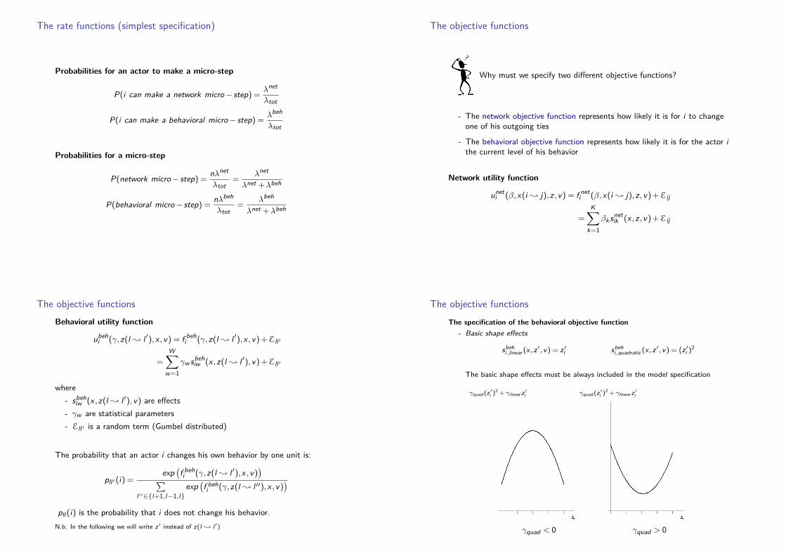
The objective functions
Why must we specify two different objective functions?
- The network objective function represents how likely it is for i to changeone of his outgoing ties
- The behavioral objective function represents how likely it is for the actor ithe current level of his behavior
Network utility function
uneti (β,x(i ; j),z,v) = f net
i (β,x(i ; j),z,v) +Eij
=
K∑k=1
βk snetik (x ,z,v) +Eij
The objective functionsBehavioral utility function
ubehi (γ,z(l ; l ′),x ,v) = f beh
i (γ,z(l ; l ′),x ,v) +Ell′
=
W∑w=1
γw sbehiw (x ,z(l ; l ′),v) +Ell′
where- sbeh
iw (x ,z(l ; l ′),v) are effects- γw are statistical parameters- Ell′ is a random term (Gumbel distributed)
The probability that an actor i changes his own behavior by one unit is:
pll′(i) =exp(
f behi (γ,z(l ; l ′),x ,v)
)∑l′′∈l+1,l−1,l
exp(
f behi (γ,z(l ; l ′′),x ,v)
)pll (i) is the probability that i does not change his behavior.
N.b. In the following we will write z′ instead of z(l ; l′)
The objective functionsThe specification of the behavioral objective function
- Basic shape effects
sbehi linear (x ,z ′,v) = z ′i sbeh
i quadratic (x ,z ′,v) = (z ′i )2
The basic shape effects must be always included in the model specification
γquad (z′i )2 +γlinear z′i γquad (z′i )2 +γlinear z′i
γquad < 0 γquad > 0

The objective functions
The specification of the behavioral objective function
- Classical influence effects
1. The average similarity effect
sbehi avsim(x ,z ′,v) =
1xi+
n∑j=1
xij (simz′(ij)− simz )
where
simz′(ij) = 1−
∣∣z ′i − z ′j∣∣
RzRz is the range of the behavior z and simz is the mean similarityvalue
2. The total similarity effect
sbehi totsim(x ,z ′,v) =
n∑j=1
xij (simz′(ij)− simz )
N.b.: z′j = zj
The objective functions
The specification of the behavioral objective function
- Classical influence effects
1. The average similarity effect
sbehi avsim(x ,z ′,v) =
1(n∑
j=1xij
) n∑j=1
xij (simz′(ij)− simz )
where
simz′(ij) = 1−
∣∣z ′i − z ′j∣∣
RzRz is the range of the behavior z and simz is the mean similarityvalue
2. The total similarity effect
sbehi totsim(x ,z ′,v) =
n∑j=1
xij (simz′(ij)− simz )
N.b.: z′j = zj
The objective functions
The specification of the behavioral objective function
- Position-dependent influence effects
Network position could also have an effect on the behavior of dynamics
1. outdegree effect
sbehi out (x ,z ′,v) = z ′i
n∑j=1
xij
2. indegree effect
sbehi ind (x ,z ′,v) = z ′i
n∑j=1
xji
- Effects of other actor variables.For each actor’s attribute a main effect on the behavior can be included inthe model
Simulating the co-evolution of networks and behavior
Aim: given (x ,z)(t0) and fixed parameter values, provide (x ,z)sim(t1)according to the process behind the SAOM
⇓
reproduce a possible series of network and behavior micro-stepsbetween t0 and t1
Input
n = number of actorsλnet = network rate parameter (given)λbeh = behavior rate parameter (given)β = (β1, . . . ,βK ) = objective function parameters (given)γ = (γ1, . . . ,γW ) = objective function parameters (given)(x ,z)(t0) = network and behavior at time t0 (given)
Output
(x ,z)sim(t1) = network and behavior at time t1

Simulating the co-evolution of networks and behavior
Algorithm 2:Input: x(t0), z(t0), λnet , λbeh, β, γ, nOutput: x sim(t1), zsim(t1)t← 0; x ← x(t0); z ← z(t0)while condition=TRUE do
dtnet ∼ Exp(nλnet )
dtbeh ∼ Exp(nλbeh)
if mindtnet ,dtbeh= dtnet theni ∼ Uniform(1, . . . ,n),j ∼ Multinomial(pi1, . . . ,pin)if i 6= j then
x ← x(i ; j)t← t + dtnet
elsei ∼ Uniform(1, . . . ,n),l ′ ∼ Multinomial(pl(l−1),pll′ ,pl(l+1))
if l 6= l ′ thenz ← z(l ; l ′)t← t + dtbeh
x sim(t1)← xzsim(t1)← zreturn x sim(t1), zsim(t1)
(x ,z)(t0)
n = 4
λnet = 1.5λnet = 1
β = (βout ,βrec ,βtrans )βi=(-1,0.5,-0.25)γ = (γlinear ,γquadratic ,γavsim)γi=(-2,1,0.25)
Simulating the co-evolution of networks and behavior
Algorithm 2:Input: x(t0), z(t0), λnet , λbeh, β, γ, nOutput: x sim(t1), zsim(t1)t← 0; x ← x(t0); z ← z(t0)while condition=TRUE do
dtnet ∼ Exp(nλnet )
dtbeh ∼ Exp(nλbeh)
if mindtnet ,dtbeh= dtnet theni ∼ Uniform(1, . . . ,n),j ∼ Multinomial(pi1, . . . ,pin)if i 6= j then
x ← x(i ; j)t← t + dtnet
elsei ∼ Uniform(1, . . . ,n),l ′ ∼ Multinomial(pl(l−1),pll′ ,pl(l+1))
if l 6= l ′ thenz ← z(l ; l ′)t← t + dtbeh
x sim(t1)← xzsim(t1)← zreturn x sim(t1), zsim(t1)
Generating the waiting time:- dtnet for a tie change- dtbeh for a behavior change
Simulating the co-evolution of networks and behavior
Algorithm 2:Input: x(t0), z(t0), λnet , λbeh, β, γ, nOutput: x sim(t1), zsim(t1)t← 0; x ← x(t0); z ← z(t0)while condition=TRUE do
dtnet ∼ Exp(nλnet )
dtbeh ∼ Exp(nλbeh)
if mindtnet ,dtbeh= dtnet theni ∼ Uniform(1, . . . ,n)j ∼ Multinomial(pi1, . . . ,pin)if i 6= j then
x ← x(i ; j)t← t + dtnet
elsei ∼ Uniform(1, . . . ,n)l ′ ∼ Multinomial(pl(l−1),pll′ ,pl(l+1))
if l 6= l ′ thenz ← z(l ; l ′)t← t + dtbeh
x sim(t1)← xzsim(t1)← zreturn x sim(t1), zsim(t1)
Which micro-step is going tohappen?
Ifdtnet < dtbeh
then a network micro-step takesplace
The following steps are the sameof those in Algorithm 1
Simulating the co-evolution of networks and behavior
Algorithm 2:Input: x(t0), z(t0), λnet , λbeh, β, γ, nOutput: x sim(t1), zsim(t1)t← 0; x ← x(t0); z ← z(t0)while condition=TRUE do
dtnet ∼ Exp(nλnet )
dtbeh ∼ Exp(nλbeh)
if mindtnet ,dtbeh= dtnet theni ∼ Uniform(1, . . . ,n)j ∼ Multinomial(pi1, . . . ,pin)if i 6= j then
x ← x(i ; j)t← t + dtnet
elsei ∼ Uniform(1, . . . ,n)l ′ ∼ Multinomial(pl(l−1),pll′ ,pl(l+1))
if l 6= l ′ thenz ← z(l ; l ′)
t← t + dtbeh
x sim(t1)← xzsim(t1)← zreturn x sim(t1), zsim(t1)
Which micro-step is going tohappen?
Ifdtbeh < dtnet
then a behavior micro-step takesplace

Simulating the co-evolution of networks and behavior
Algorithm 2:Input: x(t0), z(t0), λnet , λbeh, β, γ, nOutput: x sim(t1), zsim(t1)t← 0; x ← x(t0); z ← z(t0)while condition=TRUE do
dtnet ∼ Exp(nλnet )
dtbeh ∼ Exp(nλbeh)
if mindtnet ,dtbeh= dtnet theni ∼ Uniform(1, . . . ,n)j ∼ Multinomial(pi1, . . . ,pin)if i 6= j then
x ← x(i ; j)t← t + dtnet
elsei ∼ Uniform(1, . . . ,n)l ′ ∼ Multinomial(pl(l−1),pll′ ,pl(l+1))
if l 6= l ′ thenz ← z(l ; l ′)
t← t + dtbeh
x sim(t1)← xzsim(t1)← zreturn x sim(t1), zsim(t1)
Select the actor i who has the op-portunity to change his behavior
e.g. i=1
(x ,z)(t0)
Simulating the co-evolution of networks and behavior
Algorithm 2:Input: x(t0), z(t0), λnet , λbeh, β, γ, nOutput: x sim(t1), zsim(t1)t← 0; x ← x(t0); z ← z(t0)while condition=TRUE do
dtnet ∼ Exp(nλnet )
dtbeh ∼ Exp(nλbeh)
if mindtnet ,dtbeh= dtnet theni ∼ Uniform(1, . . . ,n)j ∼ Multinomial(pi1, . . . ,pin)if i 6= j then
x ← x(i ; j)t← t + dtnet
elsei ∼ Uniform(1, . . . ,n)l ′ ∼ Multinomial(pl(l−1),pll′ ,pl(l+1))
if l 6= l ′ thenz ← z(l ; l ′)
t← t + dtbeh
x sim(t1)← xzsim(t1)← zreturn x sim(t1), zsim(t1)
Select the level l ′ towards i isgoing to adjust his behavior
l → l ′ f behi pll′
2 → 1 0.017 0.0172 → 2 0.052 0.0523 → 3 0.930 0.931
Simulating the co-evolution of networks and behavior
Algorithm 2:Input: x(t0), z(t0), λnet , λbeh, β, γ, nOutput: x sim(t1), zsim(t1)t← 0; x ← x(t0); z ← z(t0)while condition=TRUE do
dtnet ∼ Exp(nλnet )
dtbeh ∼ Exp(nλbeh)
if mindtnet ,dtbeh= dtnet theni ∼ Uniform(1, . . . ,n)j ∼ Multinomial(pi1, . . . ,pin)if i 6= j then
x ← x(i ; j)t← t + dtnet
elsei ∼ Uniform(1, . . . ,n)l ′ ∼ Multinomial(pl(l−1),pll′ ,pl(l+1))
if l 6= l ′ thenz ← z(l ; l ′)
t← t + dtbeh
x sim(t1)← xzsim(t1)← zreturn x sim(t1), zsim(t1)
Select the level l ′ towards i is go-ing to adjust his behavior
e.g. l’=3
(x ,z(l → l ′))
Simulating the co-evolution of networks and behavior
Algorithm 2:Input: x(t0), z(t0), λnet , λbeh, β, γ, nOutput: x sim(t1), zsim(t1)t← 0; x ← x(t0); z ← z(t0)while condition=TRUE do
dtnet ∼ Exp(nλnet )
dtbeh ∼ Exp(nλbeh)
if mindtnet ,dtbeh= dtnet theni ∼ Uniform(1, . . . ,n)j ∼ Multinomial(pi1, . . . ,pin)if i 6= j then
x ← x(i ; j)t← t + dtnet
elsei ∼ Uniform(1, . . . ,n)l ′ ∼ Multinomial(pl(l−1),pll′ ,pl(l+1))
if l 6= l ′ thenz ← z(l ; l ′)
t← t + dtbeh
x sim(t1)← xzsim(t1)← zreturn x sim(t1), zsim(t1)

Simulating the co-evolution of networks and behavior
1. Unconditional simulation:simulation carries on until a predetermined time length has elapsed(usually until t = 1).
2. Conditional simulation on the observed number of changes:- simulation runs on until
n∑i,j=1ı 6=j
∣∣∣X obsij (t1)−Xij (t0)
∣∣∣=
n∑i,j=1
∣∣∣X simij (t1)−Xij (t0)
∣∣∣
- simulation runs on untiln∑
i=1
∣∣∣zobsi (t1)− zi (t0)
∣∣∣=
n∑i=1
∣∣∣zsimi (t1)− zi (t0)
∣∣∣
Example
Example data: excerpt from the “Teenage Friends and Lifestyle Study” data set
We will use the SAOM for the co-evolution of networks and behaviors todistinguish influence from selection.
1. Do pupils select friends based on similar smoking behavior?
2. Are pupils influenced by friends to adjust to their smoking behavior?
Dependent variables: friendship networks and smoking behavior
Covariate: gender
Precondition of the analysis
To find out whether it makes sense to analyze the data with a co-evolutionmodel one should check whether:
1. the data are sufficiently informative
J =N11
N11 + N01 + N10> 0.3 Jaccard index
Precondition of the analysis
2. there is interdependence between network and behavioral variables
I =
n∑
ijxij (zi − z)(zj − z)(∑
ijxij
)(∑i
(zi − z)2
) Moran index
where z is the mean of z over all the periods

Precondition of the analysis
The computation of the index I for the data leads to
0.244 0.258 0.341
Conclusion:there is considerable dependence between networks and behaviorsand it is reasonable to apply the SAOM
moran1 <- nacf(net1,tobacco[,1],lag.max=1,neighborhood.type = ”out”,type=”moran”,mode=”digraph”)
moran2 <- nacf(net2,tobacco[,2]„lag.max=1,neighborhood.type = ”out”,type=”moran”,mode=”digraph”)
moran3 <- nacf(net3,tobacco[,3]„lag.max=1,neighborhood.type = ”out”,type=”moran”,mode=”digraph”)
moranInd <- c(moran1[2],moran2[2],moran3[2])
Parameter interpretation: a baseline model
Estimates s.e. t-scoreNetwork Dynamicsconstant friendship rate (period 1) 8.6287 ( 0.6666 )constant friendship rate (period 2) 7.2489 ( 0.5466 )
outdegree (density) -2.4084 ( 0.0407 ) -59.1268reciprocity 2.7024 ( 0.0823 ) 32.8337
Behavior Dynamicsrate smokebeh (period 1) 3.8922 ( 1.9689 )rate smokebeh (period 2) 4.4813 ( 2.3679 )
behavior smokebeh linear shap -3.5464 ( 0.4394 ) -8.0712behavior smokebeh quadratic shape 2.8464 ( 0.3628 ) 7.8447
Network rate parameters:- about 9 opportunities for a network change in the first period- about 7 opportunities for a network change in the second period
Parameter interpretation: a baseline model
Estimates s.e. t-scoreNetwork Dynamicsconstant friendship rate (period 1) 8.6287 ( 0.6666 )constant friendship rate (period 2) 7.2489 ( 0.5466 )
outdegree (density) -2.4084 ( 0.0407 ) -59.1268reciprocity 2.7024 ( 0.0823 ) 32.8337
Behavior Dynamicsrate smokebeh (period 1) 3.8922 ( 1.9689 )rate smokebeh (period 2) 4.4813 ( 2.3679 )
behavior smokebeh linear shap -3.5464 ( 0.4394 ) -8.0712behavior smokebeh quadratic shape 2.8464 ( 0.3628 ) 7.8447
Network objective function parameters:- outdegree parameter: the observed networks have low density- reciprocity parameter: strong tendency towards reciprocated ties
Parameter interpretation: a baseline model
Estimates s.e. t-scoreNetwork Dynamicsconstant friendship rate (period 1) 8.6287 ( 0.6666 )constant friendship rate (period 2) 7.2489 ( 0.5466 )
outdegree (density) -2.4084 ( 0.0407 ) -59.1268reciprocity 2.7024 ( 0.0823 ) 32.8337
Behavior Dynamicsrate smokebeh (period 1) 3.8922 ( 1.9689 )rate smokebeh (period 2) 4.4813 ( 2.3679 )
behavior smokebeh linear shap -3.5464 ( 0.4394 ) -8.0712behavior smokebeh quadratic shape 2.8464 ( 0.3628 ) 7.8447
Behavioral rate parameters:- about 4 opportunities for a behavioral change in the first period- about 4 opportunities for a behavioral change in the second period

Parameter interpretation: a baseline model
Estimates s.e. t-scoreNetwork Dynamicsconstant friendship rate (period 1) 8.6287 ( 0.6666 )constant friendship rate (period 2) 7.2489 ( 0.5466 )
outdegree (density) -2.4084 ( 0.0407 ) -59.1268reciprocity 2.7024 ( 0.0823 ) 32.8337
Behavior Dynamicsrate smokebeh (period 1) 3.8922 ( 1.9689 )rate smokebeh (period 2) 4.4813 ( 2.3679 )
behavior smokebeh linear shap -3.5464 ( 0.4394 ) -8.0712behavior smokebeh quadratic shape 2.8464 ( 0.3628 ) 7.8447
Behavioral objective function parameters:
attractiveness of different behavioral levels based on the current structure ofthe network and the behavior of the others
Parameter interpretation: a baseline model
- Smoking behavior: coded with 1 for “no”, 2 for “occasional”, and 3 for“regular” smokers.
- The smoking covariate is centered: z = 1.377 is the mean of the covariate
zi − z =
−0.377 for no smokers
0.623 for occasional smokers
1.623 for regular smokers
- The contribution to the behavioral objective function is
γlinear (zi − z) +γquadratic (zi − z)2 =
=−3.5464(zi − z) + 2.8464(zi − z)2
Parameter interpretation: a baseline model
U-shaped changes in the behavior are drawn to the extreme of the range
A more complex model
The baseline model does not provide any information about selection andinfluence processes:
- the network dynamics are explained by the preference towards creating andreciprocating ties
- the behavior dynamics are described only by the distribution of thebehavior in the population
If we want to distinguish selection from influence we should include in theobjective functions specification:
- the effects that capture the dependence of social network dynamics onactor’s characteristic
- the effects that capture the dependence of behavior dynamics on socialnetwork

A more complex model
Effects for the dependence of network dynamics on actor’s characteristic
- pupils prefer to establish friendship relations with others that are similar tothemselves → covariate similarity
This effect must be controlled for the sender and receiver effects of thecovariate.
- Covariate ego effect
- Covariate alter effect
A more complex model
Effects for the dependence of behavior dynamics on network
- pupils tend to adjust their smoking behavior according to the behaviors oftheir friends → average similarity effect
This effect must be controlled for the indegree and the outdegree effects- Indegree effect
- Outdegree effect
A more complex model
Estimates s.e. t-scoreNetwork Dynamicsconstant friendship rate (period 1) 10.7166 ( 1.4036 )constant friendship rate (period 2) 9.0005 ( 0.7709 )
outdegree (density) -2.8435 ( 0.0572 ) -49.6776reciprocity 1.9683 ( 0.0933 ) 21.1077transitive triplets 0.4447 ( 0.0322 ) 13.7964sex ego 0.1612 ( 0.1206 ) 1.3368sex alter -0.1476 ( 0.1064 ) -1.3871sex similarity 0.9104 ( 0.0882 ) 10.3244smoke ego 0.0665 ( 0.0846 ) 0.7857smoke alter 0.1121 ( 0.0761 ) 1.4719smokebeh similarity 0.5114 ( 0.1735 ) 2.9479
Rate parameters: the speed at which tie change occur is higher than the speedat which behavioral change occur
A more complex model
Estimates s.e. t-scoreNetwork Dynamicsconstant friendship rate (period 1) 10.7166 ( 1.4036 )constant friendship rate (period 2) 9.0005 ( 0.7709 )
outdegree (density) -2.8435 ( 0.0572 ) -49.6776reciprocity 1.9683 ( 0.0933 ) 21.1077transitive triplets 0.4447 ( 0.0322 ) 13.7964sex ego 0.1612 ( 0.1206 ) 1.3368sex alter -0.1476 ( 0.1064 ) -1.3871sex similarity 0.9104 ( 0.0882 ) 10.3244smoke ego 0.0665 ( 0.0846 ) 0.7857smoke alter 0.1121 ( 0.0761 ) 1.4719smokebeh similarity 0.5114 ( 0.1735 ) 2.9479
Network objective function parameters:
tendency towards reciprocity, transitivity and homophily with respect to gender

A more complex model
Estimates s.e. t-scoreNetwork Dynamicsconstant friendship rate (period 1) 10.7166 ( 1.4036 )constant friendship rate (period 2) 9.0005 ( 0.7709 )
outdegree (density) -2.8435 ( 0.0572 ) -49.6776reciprocity 1.9683 ( 0.0933 ) 21.1077transitive triplets 0.4447 ( 0.0322 ) 13.7964sex ego 0.1612 ( 0.1206 ) 1.3368sex alter -0.1476 ( 0.1064 ) -1.3871sex similarity 0.9104 ( 0.0882 ) 10.3244smoke ego 0.0665 ( 0.0846 ) 0.7857smoke alter 0.1121 ( 0.0761 ) 1.4719smokebeh similarity 0.5114 ( 0.1735 ) 2.9479
Network objective function parameters:
pupils selected others with similar smoking behavior as friends
→ evidence for selection process
A more complex model
The contribution to the network objective function is given by:
βego(zi − z) +βalter (zj − z) +βsame(
1− |zi−zj |Rz− simz
)=
= 0.0665(zi −1.377) + 0.1121(zj −1.377) + 0.5114(1− |zi−zj |Rz−0.7415)
zi/zj no occasional regularno 0.0648 -0.0787 -0.2223occasional -0.1243 0.2435 0.0999regular -0.3135 0.0543 0.4221
- preference for similar alters- this tendency is strongest for high values on smoking behavior
A more complex model
Estimates s.e. t-scoreBehavior Dynamicsrate smokebeh (period 1) 3.9041 (1.7402 )rate smokebeh (period 2) 3.8059 ( 1.4323 )
behavior smokebeh linear shape -3.3573 ( 0.5678 ) -5.9129behavior smokebeh quadratic shape 2.8406 ( 0.4125 ) 6.8864behavior smokebeh indegree 0.1711 ( 0.1812 ) 0.9444behavior smokebeh outdegree 0.0128 ( 0.1926 ) 0.0662behavior smokebeh average similarity 3.4361 ( 1.4170 ) 2.4250
Behavioral objective function parameters:
U-shaped distribution of the smoking behavior
A more complex model
Estimates s.e. t-scoreBehavior Dynamicsrate smokebeh (period 1) 3.9041 (1.7402 )rate smokebeh (period 2) 3.8059 ( 1.4323 )
behavior smokebeh linear shape -3.3573 ( 0.5678 ) -5.9129behavior smokebeh quadratic shape 2.8406 ( 0.4125 ) 6.8864behavior smokebeh indegree 0.1711 ( 0.1812 ) 0.9444behavior smokebeh outdegree 0.0128 ( 0.1926 ) 0.0662behavior smokebeh average similarity 3.4361 ( 1.4170 ) 2.4250
Behavioral objective function parameters:
indegree and outdegree effects are not significant

A more complex model
Estimates s.e. t-scoreBehavior Dynamicsrate smokebeh (period 1) 3.9041 (1.7402 )rate smokebeh (period 2) 3.8059 ( 1.4323 )
behavior smokebeh linear shape -3.3573 ( 0.5678 ) -5.9129behavior smokebeh quadratic shape 2.8406 ( 0.4125 ) 6.8864behavior smokebeh indegree 0.1711 ( 0.1812 ) 0.9444behavior smokebeh outdegree 0.0128 ( 0.1926 ) 0.0662behavior smokebeh average similarity 3.4361 ( 1.4170 ) 2.4250
Behavioral objective function parameters:
pupils are influenced by the smoking behavior of the others
→ evidence for influence process
A more complex model
The contribution to the behavioral objective function is given by:
γlinear (zi − z) +γquadratic (zi − z)2 +γavsim1
xi+
n∑j=1
xij (simz (ij)− simz ) =
=−3.3573(zi − z) + 2.8406(zi − z)2 + 3.4361 1xi+
n∑j=1
xij (simz (ij)−0.7415)
where simz (ij) = 1− |zi−zj |RZ
= 1
Example
a) i adjusts his behavior to “no-smoker” when all of his friends are no-smokers
simz (ij) = 1− |1−1|2 = 1
−3.3573(1−1.377) + 2.8406(1−1.377)2 + 3.4361(1−0.7415) = 2.56
A more complex model
The contribution to the behavioral objective function is given by:
γlinear (zi − z) +γquadratic (zi − z)2 +γavsim1
xi+
n∑j=1
xij (simz (ij)− simz ) =
=−3.3573(zi − z) + 2.8406(zi − z)2 + 3.4361 1xi+
n∑j=1
xij (simz (ij)−0.7415)
where simz (ij) = 1− |zi−zj |RZ
= 1
Example
b) i adjusts his behavior to “no-smoker” when all of his friends are occasionalsmokers
simz (ij) = 1− |1−2|2 = 0.5
−3.3573(1−1.377) + 2.8406(1−1.377)2 + 3.4361(0.5−0.7415) = 0.84
A more complex model
The contribution to the behavioral objective function is given by:
γlinear (zi − z) +γquadratic (zi − z)2 +γavsim1
xi+
n∑j=1
xij (simz (ij)− simz ) =
=−3.3573(zi − z) + 2.8406(zi − z)2 + 3.4361 1xi+
n∑j=1
xij (simz (ij)−0.7415)
where simz (ij) = 1− |zi−zj |RZ
= 1
Example
b) i adjusts his behavior to “no-smoker” when all of his friends are regularsmokers
simz (ij) = 1− |1−3|2 = 0
−3.3573(1−1.377) + 2.8406(1−1.377)2 + 3.4361(0−0.7415) =−0.88

A more complex model
The contribution to the behavioral objective function is given by:
γlinear (zi − z) +γquadratic (zi − z)2 +γavsim1
xi+
n∑j=1
xij (simz (ij)− simz ) =
=−3.3573linear (zi − z) + 2.8406quadratic (zi − z)2 + 3.4361 1xi+
n∑j=1
xij (simz (ij)−0.7415)
zj / zi no occasional regularno 2.56 -1.82 -0.51occasional 0.84 -0.10 1.20regular -0.88 -1.82 2.92
- the focal actor prefers to have the same behavior as all these friends(except for the occasional smokers)
- friends do not smoke at all: the preference toward imitating their behavioris less strong
The parameter estimation (MoM)
Aim: given the longitudinal data
(x ,z)(t0), . . . ,(x ,z)(tM) V1, . . . ,VH
estimate the parameters for the co-evolution model
- M rate parameters for the network rate function
λnet1 , . . . , λnet
M
- M rate parameters for the behavior rate function
λbeh1 , . . . , λbeh
M
- K and W parameters for the network objective function and for thebehavior objective function, respectively
f neti (β,x ′,z,v) =
K∑k=1
βk snetik (x ′,z,v) f beh
i (γ,x ′,z,v) =
W∑w=1
γw sbehiw (x ,z ′,v)
The parameter estimation (MoM)
We can estimate the 2M + K + W -dimensional parameter θ using the MoM
In practice:
1. find 2M + K + W statistics
2. set the theoretical expected value of each statistic equal to its samplecounterpart
3. solve the resulting system of equations
Eθ[S− s] = 0
with respect to θ
The parameter estimation (MoM)
Statistics:
- Network rate parameters for the period m
snetλm (X(tm),X(tm−1)|X(tm−1)) =
n∑i,j=1
∣∣Xij (tm)−Xij (tm−1)∣∣
- Behavior rate parameters for the period m
sbehλm (Z(tm),Z(tm−1)|Z(tm−1)) =
n∑i=1
|Zi (tm)−Zi (tm−1)|
m = 1, . . . ,M
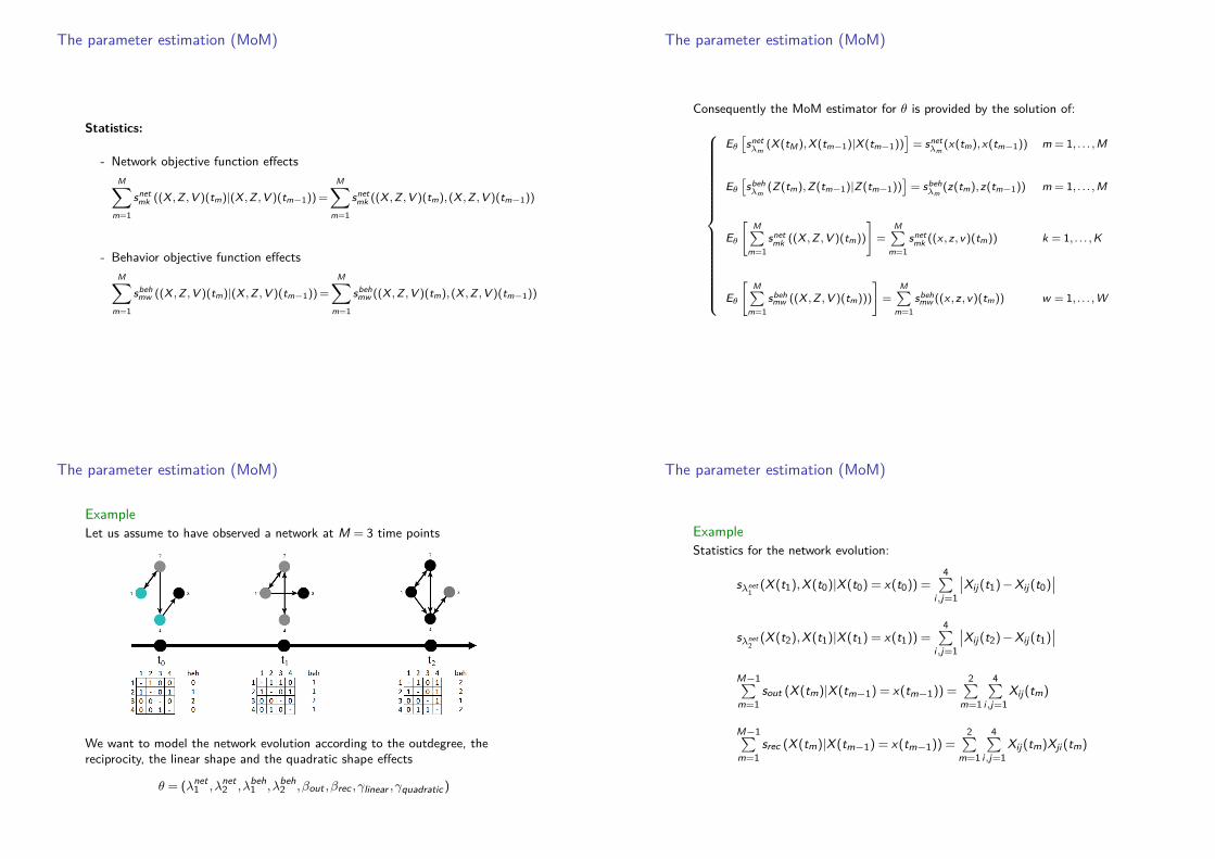
The parameter estimation (MoM)
Statistics:
- Network objective function effectsM∑
m=1
snetmk ((X ,Z ,V )(tm)|(X ,Z ,V )(tm−1)) =
M∑m=1
snetmk ((X ,Z ,V )(tm),(X ,Z ,V )(tm−1))
- Behavior objective function effectsM∑
m=1
sbehmw ((X ,Z ,V )(tm)|(X ,Z ,V )(tm−1)) =
M∑m=1
sbehmw ((X ,Z ,V )(tm),(X ,Z ,V )(tm−1))
The parameter estimation (MoM)
Consequently the MoM estimator for θ is provided by the solution of:
Eθ[
snetλm
(X(tM ),X(tm−1)|X(tm−1))]
= snetλm
(x(tm),x(tm−1)) m = 1, . . . ,M
Eθ[
sbehλm
(Z(tm),Z(tm−1)|Z(tm−1))]
= sbehλm
(z(tm),z(tm−1)) m = 1, . . . ,M
Eθ
[M∑
m=1snet
mk ((X ,Z ,V )(tm))
]=
M∑m=1
snetmk ((x ,z,v)(tm)) k = 1, . . . ,K
Eθ
[M∑
m=1sbeh
mw ((X ,Z ,V )(tm)))
]=
M∑m=1
sbehmw ((x ,z,v)(tm)) w = 1, . . . ,W
The parameter estimation (MoM)
ExampleLet us assume to have observed a network at M = 3 time points
We want to model the network evolution according to the outdegree, thereciprocity, the linear shape and the quadratic shape effects
θ = (λnet1 ,λnet
2 ,λbeh1 ,λbeh
2 ,βout ,βrec ,γlinear ,γquadratic )
The parameter estimation (MoM)
ExampleStatistics for the network evolution:
sλnet1
(X(t1),X(t0)|X(t0) = x(t0)) =4∑
i,j=1
∣∣Xij (t1)−Xij (t0)∣∣
sλnet2
(X(t2),X(t1)|X(t1) = x(t1)) =4∑
i,j=1
∣∣Xij (t2)−Xij (t1)∣∣
M−1∑m=1
sout (X(tm)|X(tm−1) = x(tm−1)) =2∑
m=1
4∑i,j=1
Xij (tm)
M−1∑m=1
srec (X(tm)|X(tm−1) = x(tm−1)) =2∑
m=1
4∑i,j=1
Xij (tm)Xji (tm)

The parameter estimation (MoM)
ExampleStatistics for the behavior evolution:
sλbeh1
(Z(t1),Z(t0)|Z(t0) = z(t0)) =4∑
i=1|Zi (t1)−Zi (t0)|
sλbeh2
(Z(t2),Z(t1)|Z(t1) = z(t1)) =4∑
i=1|Zi (t2)−Zi (t1)|
M∑m=1
slinear (Z(tm)|Z(tm−1) = z(tm−1)) =2∑
m=1
4∑i=1
zi (tm)
M∑m=1
squadratic (Z(tm)|Z(tm−1) = z(tm−1)) =2∑
m=1
4∑i=1
z2i (tm)
The parameter estimation (MoM)
Example
sλnet1
= 3 sλnet2
= 4
sλbeh1
= 2 sλbeh2
= 4
sout = 5 + 7 = 12 srec = 4 + 6 = 10
slinear = 5 + 7 = 12 squadratic = 7 + 13 = 20
The parameter estimation (MoM)ExampleWe look for the value of θ that satisfies the system:
Eθ[
Sλnet1
]= 3
Eθ[
Sλnet2
]= 4
Eθ[
Sλbeh1
]= 2
Eθ[
Sλbeh2
]= 4
Eθ[Sout ] = 12
Eθ[Srec ] = 10
Eθ[Slinear ] = 12
Eθ[Squadratic ] = 20
The parameter estimation (MoM)
In a more compact notation, we look for the value of θ that satisfies thesystem:
Eθ[S− s] = 0
but we know that we cannot solve it analytically.
The soultion is again provided by the Robbins-Monro algorithm.

Outline
Introduction
The Stochastic actor-oriented model
Extending the model: analyzing the co-evolution of networks and behavior
Something more on the SAOM
ERGMs and SAOMs
Creating and deleting ties
Terminating a tie is not just the opposite of creating a tie
Example
- the loss in terminating a tie is greater than the reward in creating one
- transitivity plays an important role especially in creating ties
This is modeled by adding to the objective function one of the two components:
1. the creation function
2. the endowment function
The creation function
Models the gain in satisfaction incurred when a network tie is created:
ci (δ,x) =∑
k
δk sik (x)
where
- δk are statistical parameters
- sik (x) are the effects
The utility function for an actor i when he creates a new tie is provided by:
ui (x) = fi (β,x) + ci (δ,x) + εi (t,x , j)
The creation function is zero for the dissolution of ties
The endowment function
Models the loss in satisfaction incurred when a network tie is deleted
ei (η,x) =∑
k
ηk sik (x)
where
- ηk are statistical parameters
- sik (x) are the effects
The utility function for an actor i when he deletes a tie is provided by:
ui (x) = fi (β,x) + ei (η,x) + εi (t,x , j)
The endowment function is zero for the creation of ties

Creating and deleting ties - Remarks
- creation and deletion functions must not be included when ties mainly arecreated or terminated
- it could also happen that increasing a behavior is not the same asdecreasing a behavior. Thus, there are also:
1. the creation behavior function
2. the endowment behavior function
but their usage is still under investigation
Creating and deleting ties
ExampleExample data: excerpt from the “Teenage Friends and Lifestyle Study” data set
We estimate the SAOM for investing the evolution of friendship networksaccording to:
- outdegree- reciprocity- transitivity- reciprocity for the endowment function
myeff < − includeEffects(myeff,transTrip)myeff < − includeEffects(myeff,recip,type=”endow”)myeffmymodel < − sienaModelCreate(useStdInits = FALSE, projname = ’tfls’)model1 < − siena07(mymodel, data = mydata, effects=myeff,useCluster=TRUE,nbrNodes=2, initC=TRUE,clusterString=rep(”localhost”, 2))
Creating and deleting ties
Example
Estimates s.e. t-scoreRate parameters:Rate parameter period 1 6.70 0.73Rate parameter period 2 5.81 0.58
Other parameters:outdegree -2.58 0.05 -51.62reciprocity 3.23 0.29 11.15reciprocity (endow) 2.23 0.58 3.85transitive triplets 0.44 0.03 14.55
The utility function for an actor i when he deletes a tie is provided by:
ui (x) = fi (β,x) + ei (η,x) + εi (t,x , j) =
= βout si out (x) +βrec si rec (x) +βtrans si trans (x) +ηrec si rec (x)
= −2.58si out (x) + 3.23si rec (x) + 0.44si trans (x)−2.23si rec (x)
Creating and deleting ties
Example
Estimates s.e. t-scoreRate parameters:Rate parameter period 1 8.44 0.73Rate parameter period 2 7.09 0.58
Other parameters:outdegree -2.58 0.05 -51.62reciprocity 3.23 0.29 11.15reciprocity (endow) 2.23 0.58 3.85transitive triplets 0.44 0.03 14.55
Ties formation/deletion
-2.58
+2.58
Creating and deleting ties
Example
Estimates s.e. t-scoreRate parameters:Rate parameter period 1 8.44 0.73Rate parameter period 2 7.09 0.58
Other parameters:outdegree -2.58 0.05 -51.62reciprocity 3.23 0.29 11.15reciprocity (endow) 2.23 0.58 3.85transitive triplets 0.44 0.03 14.55
Reciprocation/ending reciprocation
+0.65
-2.88
Creating and deleting ties
Example
Ties formation/deletion-2.58
+2.58
Reciprocation/ending reciprocation+0.65
-2.88
Conclusions:
1. formation of reciprocal ties is more rewarding than the formation of anon-reciprocal tie
2. dissolution of reciprocal ties is more costly than the dissolution of anon-reciprocal tie and the creation of a reciprocal tie

Non-directed relations
For directed relation we assumed that:
1. an actor gets the opportunity to make a change
2. he decided for the change that assures him the highest payoff
Are this assumptions still reliable when we consider undi-rected relations such as: collaboration, trade, strategicalliance?
- Yes, if one actor (dictator) can impose a decisionabout a tie to another
- No, if there is coordination or negotiation about atie
Non-directed relations
1. Dictatorial choice: i chooses his action and imposes his decision to j
Actor 1 gets the opportunity to change
Non-directed relations
1. Dictatorial choice: i chooses his action and imposes his decision to j
Actor 1 evaluates the alternatives and the corresponding objective functions
Non-directed relations
1. Dictatorial choice: i chooses his action and imposes his decision to j
E.g. actor 1 imposes his choice to actor 2

Non-directed relations
2. Mutual agreement: both actors must agree
Actor 1 gets the opportunity to change
Non-directed relations
2. Mutual agreement: both actors must agree
Actor 1 evaluates the alternatives and the corresponding objective functions
Non-directed relations
2. Mutual agreement: both actors must agree
Actor 1 suggests to modify the tie towards actor 2
Non-directed relations
2. Mutual agreement: both actors must agreeActor 2 evaluates the proposal of actor 1
and accepts it with probability
P(2 accepts tie proposal) =exp(f2(x+12))
exp(f2(x+12)) + exp(f2(x−12))

Non-directed relations - Tie-based approachA couple (i , j) of actors is selected with rate λij and gets the opportunity torevise the tie among them
1. Dictatorial choice: one actor can impose the decision (e.g. actor 1)
Actor 1 chooses his action with probability
P(1 imposes a tie on 2) =exp(f1(x+12))
exp(f1(x+12) + f1(x−12))
Non-directed relations - Tie-based approachA couple (i , j) of actors is selected with rate λij and gets the opportunity torevise the tie among them
1. Dictatorial choice: one actor can impose the decision (e.g. actor 1)
Actor 1 chooses his action with probability
P(1 imposes a tie on 2) =exp(f1(x+12))
exp(f1(x+12)) + exp(f1(x−12))
Non-directed relations - Tie-based approach
A couple (i , j) of actors is selected with rate λij and gets the opportunity torevise the tie among them
2. Mutual agreement: both actors propose a tie
Actor 1 and 2 created a tie with probability
P(+12) =exp(f1(x+12))
exp(f1(x+12)) + exp(f1(x−12))
exp(f2(x+12)
exp(f2(x+12)) + exp(f2(x−12))
Non-directed relations - Tie-based approachA couple (i , j) of actors is selected with rate λij and gets the opportunity torevise the tie among them
3. Compensatory: the decision is made on the combined interest
Actor 1 and 2 choose their action with probability
P(+12) =exp(f1(x+12) + f2(x+12))
exp(f1(x+12) + f2(x+12)) + exp(f1(x−12) + f2(x−12))
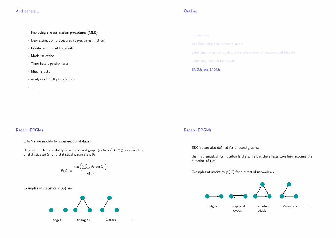
And others...
- Improving the estimation procedures (MLE)
- New estimation procedures (bayesian estimation)
- Goodness of fit of the model
- Model selection
- Time-heterogeneity tests
- Missing data
- Analysis of multiple relations
- ...
Outline
Introduction
The Stochastic actor-oriented model
Extending the model: analyzing the co-evolution of networks and behavior
Something more on the SAOM
ERGMs and SAOMs
Recap: ERGMs
ERGMs are models for cross-sectional data:
they return the probability of an observed graph (network) G ∈ G as a functionof statistics gi (G) and statistical parameters θi
P(G) =exp(∑k
i=1 θi ·gi (G))
κ(θ)
Examples of statistics gi (G) are:
edges triangles 2-stars ...
Recap: ERGMs
ERGMs are also defined for directed graphs:
the mathematical formulation is the same but the effects take into account thedirection of ties
Examples of statistics gi (G) for a directed network are:
edges reciprocal transitive 2-in-stars ...dyads triads

Recap: SAOMs
SAOMs are models for longitudinal data:
SAOMs try to explain the evolution of the network over time, assuming thatnetwork changes happen according to a continuous-time Markov chainmodeled by:
- the rate function λ- the objective function
fi (β,x(i ; j),vi ,vj ) =
K∑k=1
βk sik (x(i ; j))
where the statistics sik (x(i ; j)) are:
edges reciprocal transitive 2-in-stars ...dyads triads
SAOMs and ERGMs
Although ERGMs and SAOMs have different aims andrequire different data, the same statistics are used asexplanatory variables in both models.
This might suggest the existence of a“statistical” relation between ERGMs and SAOMs
We are going to prove that:1. ERGMs are the limiting distribution of the process
described by a certain specification of SAOMs2. ERGMs are the limiting distribution of the process
described by a tie-based version of SAOMs
Background: intensity matrix
Definition
Let X(t), t ∈ T be a continuous-time Markov chain whose transitionprobabilities are defined by:
P(X(tj ) = x |X(t) = x(t),∀t ≤ ti ) = P(X(tj ) = x |X(ti ) = x)
for each pair (x , x).
There exists a function q : X×X→ R such thatq(x , x) = lim
dt→0P(X(t+dt)=x |X(t)=x)
dt
q(x ,x) = limdt→0
P(X(t+dt)=x |X(t)=x)−1dt
The function q is called intensity matrix of the process.
The element q(x , x) is referred to as the rate at which the process in state xtends to change into x
Background (recall):limiting distribution
Definition
The limiting distribution P of a continuous-time Markov chain X(t), t ∈ Tis defined as
Px = limt→∞
P(X(tj ) = x |X(ti ) = x)
Therefore, the limiting distribution of X(t), t ∈ T is the distribution thatdescribes the probability of jumping from x to x in the long run behavior of theprocess .
Px is also the stationary distribution of the process

Background (recall):irreducible aperiodic Markov chain and limiting distribution
Definition
A continuous-time Markov chain is irreducible if there is a path between anystates x and x
A continuous-time Markov chain is aperiodic greatest common divisor of thelength of all cycles equals one.
Theorem
If X(t), t ∈ T is an irreducible and aperiodic continuous-time Markov chainand the detailed balance condition holds
Px ·q(x ,x) = Px ·q(x , x)
then Px is the unique limiting (stationary) distribution of X(t), t ∈ T
ERGMs and SAOMs
Let us now consider a particular SAOM:- objective function for each actor i
fi (β,x(i ; j)) =
K∑i=1
βk sk (x(i ; j) = β′s(x(i ; j))
- rate parameter for actor i
λi =
n∑h=1
exp(β′s(x(i ; h))
)i.e., actors for whom changed relations have a higher value, will indeedchange their relation more quickly.
ERGMs and SAOMsThe rate and the objective functions define a continuous-time Markov chain onthe set X.
The associated intensity matrix q of the process is:
q(x ,x(i ; j)) = limdt→0
P(X(t + dt) = x(i ; j)|X(t) = x)
dt= λi pij = exp(β′s(x(i ; j))
Computing the limiting distribution of SAOMs
We can prove that ERGMs
P(X = x) =
exp( K∑
i=1βk sk (x)
)κ(θ)
=exp(β′s(x))
κ(θ)
are the unique stationary distribution of the SAOM defined before
Proof
1. Existence of a unique invariant distribution- q is irriducible: each network configuration can be reached from any other
network configuration in a finite number of steps- q is aperiodic: at each time point t an actor i has the opportunity not to
change anything and, thus, the period of each state is equal to 1

Computing the limiting distribution of SAOMs
Proof (continue)
2. ERGMs are the stationary distribution of Q
In fact, given two states x and x(i ; j) of X(t), t ∈ T the balance equationholds when ERGMs is the stationary distribution:
Px(i;j) ·q(x(i ; j),x) =exp(β′s(x(i ; j))
κ(θ)· exp(β′s(x))
=exp(β′s(x))
κ(θ)· exp(β′s(x(i ; j))
= Px ·q(x ,x(i ; j))
SAOMs for non-directed relations - Tie-based approachA couple (i , j) of actors is selected with rate λij and gets the opportunity torevise the tie among them
Joint decision: the decision is made on the payoff deriving from the tie
Actor 1 and 2 choose their action with probability
p(x+12) =exp(f12(x+12)
exp(f12(x+12)) + exp(f12(x−12))
SAOMs for non-directed relations - Tie-based approach
We assume that- each dyad (i , j) can be selected with the same rate λ- the objective function is:
fij (β,x) =
k∑i=1
βk sijk (x) = β′sij x
where sijk (x) are statistics such as
edges triangles 2-stars ...
but considered from the point of view of each pair (i , j) instead of thepoint view of a certain actor.
SAOMs for non-directed relations - Tie-based approach
Assuming that at each time point only one pair (i , j) can be selected,the rate function λ and the objective function fij (β,x) definea continuous time Markov-chain with intensity matrix Q:
q(x ,x+ij ) = λp(x+ij ) = λexp(β′sij (x+ij )
exp(β′sij (x+ij ))+exp(β′sij (x−ij ))
q(x ,x−ij ) = λp(x−ij ) = λexp(β′sij (x−ij )
exp(β′sij (x+ij ))+exp(β′sij (x−ij ))
The limiting distribution of q is again ERGMs

Computing the limiting distribution of tie-based SAOMs
Proof
1. Existence of a unique invariant distribution
- q is irriducible: each network configuration can be reached from any othernetwork configuration in a finite number of steps
- q is aperiodic: at each time point t a pair (i , j) has the opportunity not tochange anything and, thus, the period of each state is equal to 1
Computing the limiting distribution of SAOMs
Proof (continue)
2. ERGMs are the stationary distribution of Q
In fact, given the two states x−ij and x+ij of X(t), t ∈ T the balanceequation holds when ERGMs is the stationary distribution:
Px−ij q(x−ij ,x+ij ) =eβ′s(x−ij )
κ(θ)·λ ·
eβ′sij (x+ij )
eβ′sij (x+ij ) + eβ′sij (x−ij )
=eβ′s(x−ij )−β′s(x+ij )+β′s(x+ij )
κ(θ)·
λ
1 + e(β′sij (x−ij )−β′sij (x+ij ))
=eβ′s(x+ij )
κ(θ)·λ ·
eβ′s(x−ij )−β′s(x+ij )
1 + eβ′sij (x−ij )−β′sij (x+ij )
=(∗)
eβ′s(x+ij )
κ(θ)·λ ·
eβ′sij (x−ij )
eβ′sij (x+ij ) + eβ′sij (x−ij )
= Px+ij ·q(x+ij ,x−ij )
(∗) β′s(x−ij )−β′s(x+ij )