the stability of a freely floating ship - prs.pl · pdf file2nd edition, revised and updated...
TRANSCRIPT

Technical Report No. 72
The Stability of a Freely Floating Ship
Final report
Maciej Pawłowski
2nd edition, revised and updated
Gdansk, January 2016

Last update: 26 I 2016
CONTENT
ABSTRACT ...............................................................................................................................2
1. INTRODUCTION..................................................................................................................3
2. HISTORICAL OUTLINE......................................................................................................3
3. FORMULATION OF THE PROBLEM................................................................................4
4. STABILITY CHARACTERISTICS......................................................................................8 4.1. Basic relationships .....................................................................................................8 4.2. Righting arm.............................................................................................................13 4.3. Calculation of moments of inertia............................................................................14 4.4. Metacentric radii. Axis of floatation........................................................................17 4.5. Mechanism of equi-volume inclinations..................................................................23 4.6. Properties of the GZ-curve.......................................................................................27 4.7. Cross-curves of stability...........................................................................................28
5. KINEMATICS OF A FREELY FLOATING SHIP.............................................................30
6. GZ-CURVE OF MINIMUM STABILITY..........................................................................34
7. NUMERICAL EXAMPLES................................................................................................38 7.1. Ships.........................................................................................................................39 7.2. Jack up rigs...............................................................................................................44
8. CONCLUSIONS..................................................................................................................54
ACKNOWLEDGEMENTS......................................................................................................55
REFERENCES .........................................................................................................................55
NOMENCLATURE .................................................................................................................58
Abstract
The report presents the problem of calculating the righting arms (GZ-curve) for a freely floating ship, longitudinally balanced at each heel angle. In such cases the GZ-curve is ambiguous, as it depends on the way the ship is balanced. Three cases are discussed: when the ship is balanced by rotating her around the trace of water in the midships, around a normal to the ship plane of symmetry, and around a normal to the initial waterplane, fixed to the ship, identical with minimum stability. In all these cases the direction of the righting moment in space and the area under the GZ-curves, which is the lowest possible, are preserved. Angular displacements (heel and trim) are the Euler's angles related to the relevant reference axis. The most important features of the GZ-curve with free trim are provided. Exemplary cal-culations illustrate how the way of balancing affects the GZ-curves.
This report concludes the theory presented in the PRS Technical Reports No 34/99, 46/02 and
in publication [7].

Technical Report No. 72
3
1. INTRODUCTION
The GZ-curve is the basis for the assessment of ship stability. For intact ships classification societies require the GZ-curve to be calculated at level keel. Until recently however, they did not clearly state which mode of calculations should be employed for damaged ships, which often led to significant discrepancies in the calculated GZ-curves.
For the intact ship it is practically meaningless which mode of calculations is employed: fixed trim, constant during heeling, or varying trim as for a freely floating ship, which changes trim depending on longitudinal equilibrium. This is due to a minor asymmetry of the ship relative to the midships. However, for the damaged ship the mode of calculations proves to be impor-tant, as it markedly affects the GZ-curve after the immersion of the deck edge in water (Figure 1). The righting arm GZ means here the distance between the lines of action of buoyancy and gravity forces at a given heel angle in still water.
0.0
0.1
0.2
0.3
0.4
0.5
0.6
0.7
0 10 20 30 40 50 60
constant trim
free trim
GZ (m)
φ (degrees )
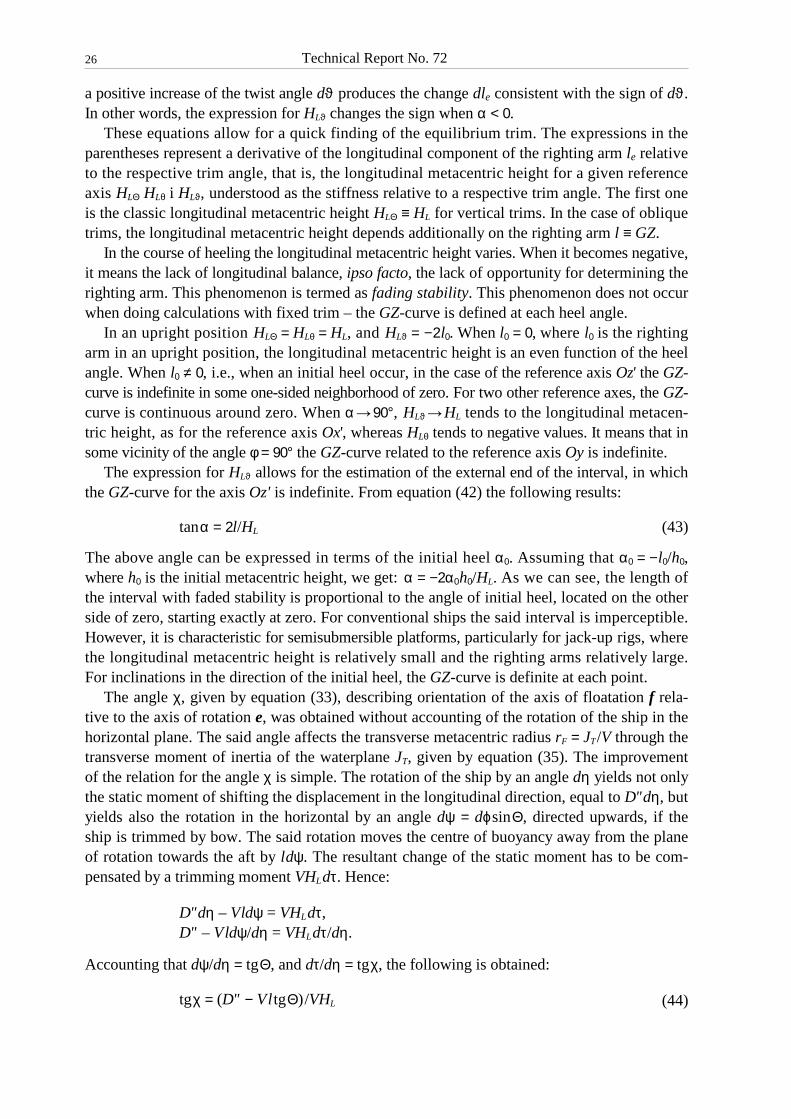
Figure 1. Effect of the GZ-curve calculation mode for a damaged platform [1]
In the case of flooding end compartments the influence of the calculations mode is particu-larly important due to the high longitudinal asymmetry of the waterplane and the small angle of deck edge immersion in the water. This influence strongly increases with the decrease of the ratio L/B. Hence, this impact increases for catamarans, SWATH (small waterplane area twin hulls), semi-submersible platforms, and jack-up rigs.
It can be demonstrated, which will be shown later, that the GZ-curve with free trim is equal to or smaller than that for a fixed trim, as shown in Figure 1. For this reason, the GZ-curve should be obligatorily calculated for a freely floating ship. In such cases, however, we face the problem of understanding the angle of heel, as it is then an ambiguous notion, manifested in various definitions of this angle and, hence, various GZ-curves.
The stability of a freely floating ship is a relatively new issue, explored mainly by Vassalos et al [2], van Santen [3], the author [4–7], and others.
2. HISTORICAL OUTLINE
Why a body floats in liquids had already been known in antiquity since the times of Archimedes (around 287–212 BC). However, how to assess and investigate the stability of floating bodies had not been known until the discovery of the Newtonian laws. In 1746 Bouguer introduced the notion of the metacentre and the metacentric height as a measure of initial stability [8]. In 1749 Euler delivered the equation for the metacentric radius, and a theorem on the equi-volume waterplanes. In 1796 Atwood published a method for calculating the righting arm for a given
Technical Report No. 72
4
heel angle, based on a shifted wedge volume method [9, 10]. From this method it follows that freeboard is crucial for the stability of ships. Nonetheless, for over a hundred years only the initial metacentric height h0 ≡ GM was used for assessing ship stability. It is stability related accidents at the end of the XIX century that led to a conclusion that the use of the GM as the sole criterion is far insufficient for the appraisal of stability, and pointed to the importance of freeboard and the GZ-curve.
The metacentric height, which otherwise is an important index of stability, allows neither for direct estimation of the stability range, nor the maximum righting lever. In this context the widely described sinking of HMS Captain in 1870 is worth mentioning, with her metacentric height of h0 = 0.79 m [11]. The ship capsized during a storm in the Bay of Biscay, whereas the ac-companying battleship Monarch of a similar size and characteristics, survived the storm un-harmed, despite a smaller metacentric height h0 = 0.73 m. The fact was very surprising for the naval architects at that time. It is very easy to explain the accident, if one observes the very different freeboards of the two ships: the Captain had a freeboard F = 1.98 m, while the Mon-arch had a freeboard F = 4.27 m. As a result, despite the smaller metacentric height, the GZ-curve of the Monarch had much better parameters than that of the Captain, whose GZmax = 0.55 m instead of 0.25 m, φmax = 40º, instead of 19º, and the range of stability φv = 70º, instead of 54º.
The Captain’s disaster gave evidence that the metacentric height alone is an insufficient measure of stability safety and made it necessary to pay attention to the stability of ships at large angles of heel. As a result, at the end of the XIX century the curve of righting arms (GZ-curve) began to be widely used for the assessment of ship stability, termed also the Reed’s curve in memory of their propagator [12]. The first GZ-based stability criteria appeared as late as in 1939, provided by Rahola [13]. These are recommendations on minimum values of some parameters related to the GZ-curve, extracted from the analyses of the GZ-curves for ships that capsized during service and for those regarded as safe. At the end of the 1960s the said criteria were adopted by IMCO (Intergovernmental Maritime Consultative Organisation, established in 1958), presently IMO (International Maritime Organisation since 1982), and they are in force until today [14].
Though the GZ-curve had been used for stability assessment of intact ships for more than a century, the stability of damaged ships until recently had been assessed with the metacentric height and freeboard. The previous SOLAS conventions were happy with the residual freeboard as low as three inches and the metacentric height of two inches. With such parameters, the GZ-curves are marginal. A change took place as late as in 1990, when the GZ-curve was standard-ised with the help of SOLAS 90 criteria [15]. However, these criteria did not provide real pro-gress, as they were introduced by purely administrative decisions, not supported by any studies. Hence, they had alleged rather than real link to actual safety in damaged condition. A breakthrough took place in 1995 with the revealing of a mechanism of ship capsizing in damaged condition [16–19]. The mechanism makes it possible to link the critical sea state and damaged stability at the moment of capsizing applying only static calculations, like for calculating the GZ-curves.
3. FORMULATION OF THE PROBLEM
Almost all widely known methods for calculating the GZ-curve assume the ship at level keel. This means indirectly that the centre of buoyancy B is supposed to be free of longitudinal dis-placements, i.e., when the ship heels it moves strictly in a frame plane. There was no need for considering earlier a different situation, as the GZ-curves were calculated solely for intact ships, for which the foregoing assumption is almost ideally valid. However, in situations when the
Technical Report No. 72
5
centre of buoyancy undergoes longitudinal displacements, which takes place when the water-plane is asymmetric with respect to the plane of rotation (i.e., of large cross-product moment), this fact cannot be any longer ignored and the calculations have to be carried out for a freely floating object, longitudinally balanced. Determination of the GZ-curve in such cases becomes ambiguous and the problem has to be fine-tuned by determining the way the ship is balanced.
It is worth emphasising that angular rotations of a freely floating object go beyond the basic ship theory. In the classic ship theory the GZ-curve is determined for a ship with fixed trim, per-forming a rotation of one degree of freedom. This is an elementary rotation, understood by everybody. Meanwhile a freely floating ship varies its trim during heeling, that is to say, it performs a rotation of two degrees of freedom, much more intricate. For this reason, and to make the calculations easier vector calculus is applied in this work.
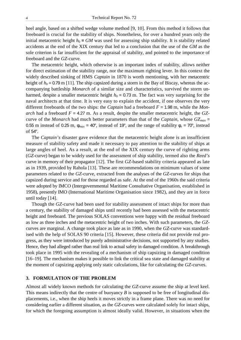
Orientation of a body in space is defined by three Euler’s angles, related to a given reference axis. In the case of a freely floating ship, two Euler’s angles are used, as the third one, describ-ing the azimuth (orientation of the ship relative to the wind direction) is irrelevant, as by defini-tion the azimuth is constant. One of the two angles plays the role of the angle of heel, while the other – the angle of trim. In the subject literature they are frequently called generalised heel and trim angles. The Euler’s angles are degrees of freedom, i.e. they can be changed independently of each other. A plane normal to the reference axis has no name in mechanics; for convenience we will call it the reference plane. One rotation is around the reference axis, and the other around the line of nodes NN, i.e. the trace of water at the plane of reference (Figure 2).
Figure 2. Euler's angles
The reference axis is customarily one of the axes of the co-ordinate system. There are then three possible reference axes, three reference planes, normal to them, and three lines of nodes. It is worth remembering, however, that a reference axis can be any axis, if necessary.
When a line of nodes is the trace of water in the midships, the Euler’s angles are related to the x-axis, normal to the midships, denoted by ϕ and Θ. The first one is the angle of heel, i.e. the angle of inclinations of the trace of water in the midships relative to the y-axis, while the other one is the trim angle, i.e. the angle of inclination of the x-axis with respect to the horizontal (sea level). The reference plane is any frame plane (station), not necessarily the midships. If the ship is trimmed in an upright position, the Euler’s angles are related to the x'-axis, normal to vertical frame planes, denoted by ϕ' and Θ'. The first one is the angle of inclinations of the trace of water in the vertical frame planes relative to the y-axis, while the other one is the angle of inclination of the x'-axis with respect to a horizontal plane. The vertical frames are deviated from the regular frames by the angle of initial trim θ0, and incline together with the ship.
Technical Report No. 72
6
When a line of nodes is the trace of water in the PS, the Euler’s angles are related to the y-axis, normal to the PS, denoted by φ and θ. The first one is the angle of heel, i.e. the angle of rotation of the PS around the trace of water, equal to the angle of inclination of the y-axis with respect to a horizontal plane (sea level), while the other one is the angle of trim, i.e. the angle of rotation of the PS around the y-axis. Contrary to the previous case, the trim of the ship in an upright position φ = 0, does not affect the meaning of the two angles of rotation.
When a line of nodes is the trace of water in the initial waterplane (waterplane in an upright position that inclines together with the ship), the Euler’s angles are related to the z'-axis, normal to the initial waterplane (when the ship in an upright position at level keel, the reference axis is the z-axis, normal to the BP). The Euler’s angles are denoted by α' and ϑ' or by α and ϑ, respec-tively. The first one is the angle of heel, i.e. the angle of rotation of the initial waterplane around the line of nodes, equal to the angle of deviation of the z'-axis from the vertical. The other one is the angle of trim, termed also the angle of twist or azimuth, i.e. the angle of rotation of the initial waterplane around the z'-axis, equal to the angle between the traces of water and PS in the initial waterplane. The reference plane is also any plane that is parallel to the initial water-plane. For a ship at level keel this can be in particular the BP.
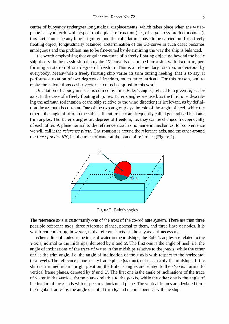
For a ship heeled with fixed trim, all the three angles of heel are the same, i.e. ϕ' = φ = α', while the trim angles vanish, i.e. Θ' = θ = ϑ' = 0. If a ship is not restrained, then at a given heel
angle, she will assume a trim to be longitudi-nally balanced. In the first case, she will trim (rotate) vertically around the trace of water in a vertical frame (Figure 3), in the second – around the y-axis (Figure 4), and in the third case – around the z'-axis (Figure 5). In the last two cases the ship trims in oblique planes.
Note that for the trim angle Θ' = 90° the angle ϕ' looses the meaning of the angle of heel, while for the angle φ = 90° the trim an-gle θ is indeterminate. Only for the reference axis Oz', both angles do not loose their mean-ing, when they assume a value 90°.
Longitudinal balance occurs when the cen-tre of buoyancy is at a vertical plane, termed the plane of rotation, passing through the cen-
tre of ship gravity. In the first case, the said plane is parallel to the line of nodes, while in the two other cases – perpendicular. As the line of nodes is fixed in space, the direction of the righting moment is also fixed in space (which does not mean it is fixed relative to the ship coordinate system). Hence, the curve of centre of buoyancy is strictly flat, lying in the plane of rotation (for a ship with fixed trim, the said curve is a projection of a spatial curve on the plane of rotation). A unit vector, normal to the plane of rotation, termed the axis of rotation, denoted further down by e, is also fixed in space.
Calculations of the GZ-curve with free trim are carried out under the following assumptions: a) The ship is inclined by a pure heeling moment, acting statically. It means that ship in-
clinations are equi-volume; b) The vector of the heeling moment is strictly horizontal. Otherwise, the heeling moment
would have a vertical component that would rotate the ship around its vertical axis; c) The vector of the heeling moment is normal to the plane of rotation. Otherwise, the ship
would not be longitudinally balanced;
G
B
Z
Figure 3. Vertical trimming of the ship

Technical Report No. 72
7
d) At each heel angle the ship is in static equilibrium, i.e. the sum of forces and moments acting on her vanish. Hence the ship's weight is equal to her buoyancy, i.e. P = D, and the static heeling moment is balanced by the righting moment of the opposite direction;
e) The righting moment is formed by a couple of forces: i.e. the gravity force applied in the ship's centre of gravity and the buoyancy force passing through the ship's centre of buoyancy. These forces are equal to each other and of opposite direction to each other. The moment vector is horizontal and normal to the plane of rotation.
The above assumptions yield some consequences:
G
B
Z
G
B
Z
Figure 4. Oblique trimming around the y-axis Figure 5. Oblique trimming around the z'-axis
1. For inclinations with fixed trim the centre of buoyancy need not be in the plane of rota-tion, therefore the moment acting on the ship has no constant direction in the horizontal plane;
2. The righting lever l ≡ GZ is the arm of the couple forming the righting moment, meas-ured in the plane of rotation; the said arm is a function of the angle of rotation η of the plane of rotation around the axis of rotation e. The angle of rotation depends on the reference axis. In the second case η ≡ φ, in the third case η ≡ α'. In the first case η < ϕ, and the relationship is more involved.
3. Since orientation of the ship relative to the plane of rotation is ambiguous, as it depends on the adopted line of nodes and related method of balancing, therefore the GZ-curves are also ambiguous. The trace of water in the PS (Figure 4) is appropriate for intact ships, as it ideal-ises the direction of the wind heeling moment. On the other hand, the edge of intersection of the initial waterplane with the waterplane is appropriate for damaged ships, where the heeling moment is created by gravitational forces, assuming minimum potential energy at the position of equilibrium. In the case of objects arbitrarily orientated to wind direction (e.g. semi-submersible units) the PS should be replaced by a wind impact screen, perpendicular to the wind direction at an initial position and rotating together with the object. The Euler's angles are related to the system Ox''y'z', fixed to the wind screen.
4. It can be seen that the projection of the y-axis on the horizontal plane is perpendicular to the trace of water in the PS. Hence, this line of nodes strictly corresponds to the direction of the heeling moment due to a shift of cargo in the ship's transverse plane. It applies also to the heel-ing moment of ro-ro vessels in damaged condition, resulting from the accumulation of water on the car deck when a symmetrical compartment has been flooded in the midships. For the same

Technical Report No. 72
8
reason the GZ-curve measured by means of the Di Belli method is strictly consistent with the above model of inclinations. In this method, a heel angle of ship model is measured, induced by shifting a weight along an arm perpendicular to the PS, identical with the inclination of the arm relative to the horizontal plane.
5. As the righting moment is all the time perpendicular to the plane of rotation, work done by the righting moment is the integral of the moment with respect to the angle of rotation of the plane of rotation η, identical with the heel angle, dependent on the line of nodes. At the same time, this is the least work which is to be performed in order to heel the ship up to a given heel angle. In other words, for the ship with fixed trim or not fully balanced, work of the righting moment is larger.
4. STABILITY CHARACTERISTICS
A number of stability characteristics, of basic importance for a freely floating ship will be dis-cussed here, such as the angle of rotation, righting arm, moments of inertia of the waterplane (understood as a cross-section of the ship hull by the flat surface of the sea), metacentric radii, axis of floatation, and cross curves of stability. We will begin by a description of the waterplane, arbitrarily inclined, which is independent of the choice of reference axis.
4.1. Basic relationships
A right hand-side co-ordinate system Oxyz, shown in Figure 6, fixed to the ship, is assumed. The origin O is identical with point K, the x-axis is directed forward, the y-axis – portside, and the z-axis – upwards. An arbitrarily inclined waterplane, as any plane can be described by the equation:
z = T0 + xtanθ + ytanϕ (1)
x
z
y
αϕ
θ
ϑ
T0
O
Figure 6. Analytical and Euler's angles of inclined waterplane
in which three independent parameters appear: the angle of inclination of the trace of water θ in the PS relative to the x-axis, the angle of inclination of the trace of water ϕ in the midships sec-tion relative to the y-axis, and the draught T0 of the z-axis. The two angles ϕ and θ are termed the analytical angles. They are positive if a positive increment of x or y corresponds to a posi-tive increment of z, as in Figure 6. Hence, the trim angle θ > 0 is positive, if the ship is trimmed by bow, while the angle ϕ > 0 is positive, when the ship is heeled portside (in Figure 3, 4 and 5 the ship is inclined to starboard, therefore the heel angles are negative in these figures). Both angles are easy to measure, as tanθ = t/Lpp, and tanϕ = ∆TLR/B, where t ≡ ∆TBS is a trim, i.e. the difference of draughts at the bow and stern perpendiculars, and ∆TLR is the difference of draughts at portside and starboard in the midships section.

Technical Report No. 72
9
The waterplane, shown in Figure 6, forms with the planes of the system a rectangular tetra-hedron of height T0, as in Figure 7, bounded by the traces of water (by the sea level). The in-clination angles θ and ϑ of the traces of water in the PS and BP relative to the x-axis are the an-gles of trim, depending on the line of nodes (the angle Θ is not shown in the figure).
x
z
y ϕ
θ
ϑ
T0
O
e1
e2
Figure 7. Tetrahedron
It is known from analytical geometry that a vector normal to the waterplane, as given by equa-tion (1), is: R = (tanθ, tanϕ, −1), which is directed downwards, and whose absolute value is:
R = √1 + tan2θ + tan2ϕ
Hence, the unit vector, normal to the waterplane, and directed upwards, equals n = −R/R. The angle between planes is the same as between vectors normal to them. Hence, the angle
α between the waterplane and BP, or an upright waterplane, is given by the equation: cosα = k ⋅ n. Therefore, cosα = 1/R = 1/(1 + tan2θ + tan2ϕ)1/2. Thus, the following is obtained:
tanα = √ tan2θ + tan2ϕ (2)
The sign of the angle α is the same as that of the angle ϕ. Taking into account that 1/R = cosα, components of the unit vector n = −R/R are as follows:
n = (−tanθ cosα, −tanϕcosα, cosα) (3)
In a similar manner it is possible to find the angle between the waterplane and PS, denoted by δ. This is an angle between the unit vectors n and −j. Hence, cosδ = −j ⋅ n = −ny = tanϕcosα.
The trim angle related to the axis Ox, i.e. the angle Θ, is equal to the angle of inclination of the x-axis relative to the surface of the sea. Hence, cos(90° + Θ) = i ⋅ n = nx, which is equivalent to sinΘ = cosαtanθ, or even simpler
tanΘ = cosϕ tanθ (4)
The angle of heel related to the trace of water in the PS, denoted by φ, is equal to the angle of inclination of the y-axis relative to the surface of the sea. Hence, cos(90° + φ) = j ⋅ n = ny, which is equivalent to sinφ = −ny = tanϕcosα, or even simpler

Technical Report No. 72
10
tanφ = cosθ tanϕ (5)
We can see that cosδ and sinφ are the same, which means that the angle of inclination of the waterplane relative to the PS is a complement of the angle φ to the right angle, i.e. δ = 90° − φ.
It is worth noting that the angle φ ≤ α, which follows immediately from the identity cosα = cosθ cosφ, which is obtained by dividing sinφ by tanφ. From equation (5) it follows moreover that the angle φ ≤ ϕ. Hence, the heel angle φ is never greater than the angle α, or the angle ϕ. However, bearing in mind that the vertical trim angle Θ is below 1°, even for the largest trim, the differences between the heel angles φ, ϕ and α are imperceptible.
The angle of inclination of the trace of water in the BP relative to the x-axis, denoted by ϑ, is the slope (gradient) of the line in a plane z = const. From equation (1) we get immediately that
tanϑ = −tanθ/tanϕ (6)
In an upright position, for ϕ = 0, equation (6) is indeterminate. In such a case ϑ = 0. Equiva-lent forms of equation (6) are as follows: sinϑ = −tanθ/tanα, cosϑ = tanϕ/tanα.
It is worth noting that traces of water in the PS and midships (or any frame plane), shown in Figure 6 and Figure 7, are not generally perpendicular one to another. The angle between them can be easily found with the help of the unit vectors of both traces e1 and e2 (Figure 7); they both look at the same directions, as the x- and y-axes. Denoting the angle between the unit vectors by β, then cosβ = e1 ⋅ e2, where the unit vector of the trace of water in the PS e1 = (cosθ, 0, sinθ), while the unit vector of traces of water at frame planes e2 = (0, cosϕ, sinϕ). Hence,
cosβ = sinθsinϕ (7)
When both analytical angles are of the same sign, the angle between the unit vectors is acute (which is also seen in Figure 6 and 7). Otherwise, the angle is obtuse.
a) Effect of the initial trim If the ship has the initial trim θ0 in an upright position, the Euler’s angles are related to the co-ordinate system Ox'yz', as in Figure 8. The axis Ox' is horizontal, i.e. parallel to the sea level, while the axis Oz' is vertical, i.e. normal to the sea level. The initial trim does not change the axis Oy. Hence, it does not change the Euler’s angles, related to this axis, while it changes them for the two other axes. As previously, we want to express them in terms of the analytical angles ϕ and θ.
x
z'
OBP
z
x'
vertical frame section
Figure 8. Co-ordinate system for a trimmed vessel
The reference plane for the axis Ox' is a vertical frame section, fixed to the ship, deviated from the regular frame planes by the initial trim angle θ0 (Figure 8); the angle θ0 > 0 is positive for bow trim. The trim angle Θ', related to the axis Ox', is equal to the angle of inclination of the axis Ox' relative to the horizontal. Hence, cos (90° + Θ') = i' ⋅ n, where i' = (cosθ0, 0, sinθ0) is a unit vector of the axis Ox'. Hence, sinΘ' = −i' ⋅ n, which yields:
Technical Report No. 72
11
sinΘ' = (tgθ cosθ0 − sinθ0)cosα (8)
If θ0 = 0, the above equation reduces to equation (4). The heel angle ϕ' is equal to the angle between traces of water and the initial waterplane at
the reference plane (vertical frame section). The unit vector of the trace of water e2' at the vertical frame section equals: e2' = n× i'/sin(90° + Θ'), while the other unit vector is identical with unit vector j of the axis Oy. Therefore, cosϕ' = j ⋅ e2', where
e2' = (n × i')/cosΘ' (9) Hence, cosϕ' = (cosθ0 + sinθ0tgθ)cosα/cosΘ' (10)
When θ0→0, ϕ'→ϕ, since cosϕ' = cosα/cosΘ. Substituting for cosΘ = cosα/cosϕ, in the limit we get cosϕ' = cosϕ, which implies ϕ' = ϕ.
The reference plane for the axis Oz' is any plane parallel to the waterplane in an upright po-sition, fixed to the ship. Its unit normal vector k' = (−sinθ0, 0, cosθ0) is identical with a unit vector of the axis Oz'. The heel angle α' is given by the equation: cosα' = k' ⋅ n, which yields:
cosα' = (1 + tanθ0tanθ)cosθ0cosα (11)
The trim angle ϑ' (twist angle) is the angle between the traces of water and PS in the reference plane (initial waterplane). The unit vectors of these traces are as follows: w = k' ×n/sinα' and i'. Hence, the twist angle is given by the equation cosϑ' = i' ⋅ w , which yields:
cosϑ' = i' ⋅ (k' ×n)/sinα' = −ny/sinα' = tanϕcosα/sinα' (12)
The sign of the angle ϑ' is opposite to the sign of the angle θ, which follows from equation (6), i.e. it is negative, when the trim is on the bow. If θ0 = 0, then α' = α, while ϑ' = ϑ, which can be easily shown. A change of the trim angle does not affect the heel angle, which is not seen at first glance. And this holds for any reference axis.
b) Wind impact screen Consider now the angles related to the wind impact plane, deviated from the PS by an angle ψ, termed the azimuth, wherein ψ > 0, if it is anti-clockwise. A system Ox''y'z' is fixed to this plane, rotated by the angle ψ around the axis Oz' relative to the system Ox'yz'. By definition, the said plane is perpendicular to the direction of the wind. When ψ = 0, it coincides with the PS.
The unit vectors i'' and j' of the system Ox''y'z' are rotated by the angle ψ relative to the unit vectors i' and j. Hence, taking their projections on the system axes, we get:
i'' = i'cosψ + j sinψ = (cosθ0cosψ, sinψ, sinθ0cosψ) j' = −i'sinψ + j cosψ = (−cosθ0sinψ, cosψ, −sinθ0sinψ)
(13)
In the case of the reference axis x'', it is easier to find the final position of the object by heeling it first by an angle ϕ' around the axis Ox'', described by the unit vector i'', and next trimming it by an angle Θ' around the trace of water in a plane normal to the axis Ox'', described by the unit vector e2'. As a result of the first rotation new unit vectors e2' and k'' are obtained:
e2' = j'cos ϕ' + k'sin ϕ' k'' = k'cos ϕ' − j'sin ϕ'
(14)
The second rotation around e2' yields the unit vector n:

Technical Report No. 72
12
n = k''cos Θ' − i''sin Θ' (15)
where the unit vectors i'' and j' are given by equations (13). The angles ϕ' and Θ' are the Euler’s angles, related to the reference axis Ox'; the latter results from longitudinal balancing of the ship.
In the case of the reference axis Oy', normal to the wind impact plane, playing a role of the reference plane, the line of nodes is the trace of water in the said plane e1'. This trace is at the same time the axis of rotation, related to the reference axis Oy'. The unit vector e1' results from trimming of the ship by the angle θ' relative to the axis Ox''. In other words, rotating the unit vectors i'' and k' by the angle θ' around the axis Oy' the unit vector i'' becomes the unit vector e1', and k' becomes k''. Hence,
e1' = i''cos θ' + k'sin θ' k'' = k'cos θ' − i''sin θ'
(16)
Finally, the unit vector n results from the rotation of the ship (waterplane) around the trace of water in the wind impact plane e1' by an angle of heel φ', i.e. the angle of inclination of the y'-axis relative to the horizontal. Hence,
n = k''cos φ' − j'sin φ' (17)
The angles θ' and φ' are the Euler angles, related to the reference axis Oy'. The former results from longitudinal balancing of the ship. When ψ = θ0 = 0, equation (17) reduces to equation (55).
For the reference axis Oz', the line of nodes is a given trace of water in the initial waterplane, playing the role of the reference plane; the unit vector of this trace is denoted by w. In an upright position, w = i'. It is at the same time the axis of rotation e, related to this axis of reference. Obviously, w = k' ×n/sinα'. It would seem that this equation cannot be used now, as the unit vector n is treated here as given, while the unit vector w is resultant, whereas it should be the other way round.
Note that in the case of the reference axes Ox'' and Oy' the azimuth is fixed in the course of longitudinal balancing of the ship. However, the situation is different in the case of the refer-ence axis Oz', the trim angle ϑ', identical with the azimuth (Figure 6), varies. When the ship is longitudinally balanced, for a given heel angle α' the azimuth is the same, irrespective of the direction of the axis of rotation e (the trace w) at an upright position. Hence, the reference axis Oz' is not related either to the wind impact screen or PS.
Nonetheless, it is worth to know the unit vectors n and w in terms of the Euler’s angles α' and ϑ'. They are essential, if one would like to find stability characteristics for an unbalanced ship. The unit vector n results from the rotation of the ship (waterplane) around the trace of water w on the initial waterplane by a heel angle α', whereas the unit vector w of the trace of water on the initial waterplane results from the rotation of w around the unit vector k' by a trim (twist) angle ϑ' (Figure 2). They are given by equations for the rotation of a vector by a given angle in an appropriate base of unit vectors:
n = k'cosα' + (w × k')sinα' w = i''cosϑ' + j'sinϑ'
(18)
where the unit vectors i'' and j' are given by equations (13), α' is the angle of heel, i.e. the angle of inclination of the initial waterplane relative to the horizontal, and ϑ' is the trim angle measured in the initial waterplane from the direction i'' (when ϑ' > 0, the twist is by aft); these are the Euler angles, related to the axis Oz'. The angle ϑ' results from longitudinal balancing of the ship. The
Technical Report No. 72
13
knowledge of the unit vector n defines the analytical angles, essential for calculating the geomet-ric characteristics of the waterplane and ship’s hull.
The unit vector w is rotated in relation to the unit vector i' by the angle Ψ = ψ + ϑ', equal to the sum of the azimuth and the angle of trim (twist). Hence, both unit vectors in equation (18) can be more simply expressed in the base of the system Ox'yz':
n = i'sinα'sinΨ − jsinα'cosΨ + k'cosα' w = i'cosΨ + jsinΨ
(19)
In view of the fact that the rotation of the unit vector w by an angle Ψ relative to i' can take place in a horizontal initial waterplane before heeling, van Santen calls this rotation the “twist” [21], without a clear indication that this is one of the two Euler’s angles, related to trim, meas-ured in the initial waterplane after heeling (Figure 5).
The following identities result from equations (18) and (19): k' ⋅ n = cosα', k' ×n = wsinα', i' ⋅ w = cosΨ, i' ×w = k'sinΨ. When ψ = 0, Ψ = ϑ'. For a trimmed ship in an upright position equations (18) yield:
w = (cosϑ', sinϑ', 0) n = (sinϑ'sinα', −cosϑ'sinα', cosα')
(20)
For a ship at level keel, the angles α' and ϑ' are replaced by α and ϑ. The unit vector n be-comes then identical with equation (54).
A change of orientation of the object in the horizontal plane introduces a third Euler an-gle – the azimuth ψ. However, it follows from equations (19) that at least for the axis Oz' the unit vector n, describing the attitude of the ship relative to the horizontal, depends on two Euler’s angles: the heel angle α' and twist (azimuth) Ψ = ψ + ϑ'. For other reference axes things are more complicated – the unit vector n depends on three Euler’s angles, not on two. It means that in such cases the relationship between the two Euler’s angles (heel and trim) and analytical angles ϕ and θ is affected additionally by the azimuth ψ.
4.2. Righting arm
The plane of rotation at which the ship is balanced is defined by a unit vector e, stationary in space, normal or parallel to the line of nodes, depending on the reference axis. When the line of nodes is the trace of water in the midships (Figure 3), the axis of rotation
e = e2 × n (21)
where e2 = (0, cosϕ, sinϕ) is a unit vector of the trace of water in the midships. When the ship has an initial trim, the unit vector e2 is replaced by the vector e2', given by equation (9), and when the azimuth ψ ≠ 0, the unit vector e2 is replaced by e2', given by equation (14). When the line of nodes is the trace of water in the PS (Figure 4), e = e1, where e1 = (cosθ, 0, sinθ) is a unit vector of the trace of water in the PS, and when the line of nodes is the trace of water in the wind impact plane, the rotation axis e = e1', where e1' is given by equation (16). When the line of nodes is the trace of water in the initial waterplane w (Figure 5), the rotation axis e = w, where the unit vector w is given by equation (18), valid both for the ship at level keel, trimmed at an upright position, or rotated by a certain azimuth ψ.
The three axes of rotation diverge, if trim varies in the course of inclinations. For example, the axis of rotation e, given by equation (21), related to the reference axis Ox, is deviated from the trace of water in the PS by an angle γ1 = β − 90°, where β is the angle between the traces of

Technical Report No. 72
14
water in the midships and PS, given by equation (7). Further, the axis of rotation e = k ×n/sinα, related to the reference axis Oz, is deviated from the trace of water in the PS by an angle γ3, which can be found from the equation: e1× e = sinγ3 n. Hence, sinγ3 = −sinθ/sinα. As can be seen, the axes of rotation coincide with each other, when there is no trim.
The plane of rotation rotates around the axis of rotation e, whereas the waterplane, i.e. the ship, rotates around an instantaneous axis of floatation f, oblique relative to the axis of rotation. The axis of floatation f is understood as the edge of intersection of two waterplanes inclined relative to one another at an infinitely small angle. In the case of equi-volume waterplanes it passes through the centre of floatation F, i.e. the centre of gravity of the waterplane. The above follows from the Pappus–Guldinus' theorem, known in ship theory as the Euler’s theorem on equi-volume waterplanes. This theorem says nothing about orientation of the axis of floatation, defined by a unit vector f, discussed below. In mechanics, the axis of floatation is termed the instantaneous axis of rotation. To find the axis of floatation it is necessary to know moments of inertia of the waterplane, which is not trivial in the case of a freely floating ship.
When the ship is being inclined the displacement remains constant, whereas the centre of buoyancy B moves in the plane of rotation, normal to the axis of rotation e. Hence, it has to satisfy the equation of the plane of rotation: e ⋅ r = 0, where r ≡ GB = (xB − xG, yB − yG, zB − zG) is the radius vector of the centre of buoyancy relative to the ship centre of gravity. When the centre of buoyancy is in the plane of rotation it is said that the ship is longitudinally balanced. The quantity e ⋅ r ≡ le is a longitudinal component of the righting arm, identical with a distance of the centre of buoyancy from the plane of rotation (if e ⋅ r > 0 it is forward of the plane of rota-tion). For given volume displacement V = const and angle of rotation of the plane of rotation η = const, the longitudinal component of the arm e ⋅ r is a function of trim.
The righting moment is given by the equation M = r × nD, where D = γV is the ship buoy-ancy. Vector M is parallel to the rotation axis e, hence: M = e ⋅ (r × n)D. The righting arm GZ = M/D is therefore given by the equation:
GZ = e ⋅ (r × n) (22)
It is a function of the angle of rotation η of the plane of rotation, depending on the reference axis. As can be seen, the basis for finding the GZ-curve with free trim is the knowledge of co-
ordinates of the centre of buoyancy B, the rotation axis e, dependent on the reference axis, and the normal n to the waterplane. In the case of the reference axis Oz' the result of calculations is a curve of righting arms with the lowest values, called the GZ-curve of minimum stability, introduced by Siemionov-Tiań-Szański [22].
4.3. Calculation of moments of inertia
A given ship hull is described in the Oxyz system, cut by an arbitrary plane. In ship statics the plane is the surface of the sea, whereas the cross-section itself is the waterplane. We want to find the principal moments of inertia for the said cross-section. They can be found indirectly, making use of moments of inertia for a projection of the cross-section (waterplane) on one of the co-ordinate planes (BP or PS), discussed in reference [22], or directly, by calculating geo-metrical characteristics of the cross-section with the help of traces of the waterplane in the frame planes [6].
Moments of inertia will be found by the direct method. A typical cross-section of the hull, i.e. the waterplane, is shown in Figure 9. The ξ-axis coincides with the trace of water in the PS, whereas the η-axis is normal to the unit vectors n and e1. The origin of the η-axis is at the point of intersection of the z-axis with the trace of water in the PS. The traces of the waterplane

Technical Report No. 72
15
in the frame planes, i.e. widths of the frames in the waterplane are oblique relative to the ξ-axis (trace of water in the PS); some of them are shown in Figure 9.
The angle between the unit vectors of the traces is equal to β. The ξ-axis divides a trace into two segments of lengths a and b; which can be directly measured in the frame planes. The quan-tities a and b have the meaning of the co-ordinates of the ends of the traces, measured along a trace. These co-ordinates are positive, if they are to the left of the ξ-axis, and negative, if they are to the right (Figure 9).
ξ
η b
a
e 2
e 1
s
P
ξ
ξ'
Figure 9. True view of the waterplane
Considering that the following holds between the oblique co-ordinates (ξ, s) of point P and its rectangular co-ordinates (ξ', η)
ξ' = ξ − ssin(β − 90°) = ξ + scosβ η = scos(β − 90°) = ssinβ
it is easy to find an area element δA in a waterplane strip of breadth dξ as well as its static and inertia moments in the categories of the oblique co-ordinates (ξ, s). These are:
δA = dξdη = dξdssinβ δMξ = ηδA = dξsdssin2β δMη = ξ'δA = ξdξdssinβ + dξsdssinβcosβ δD = ξ'ηδA = ξdξsdssin2β + dξs2dssin2βcosβ δJξ = η2δA = dξs2dssin3β δJη = ξ'2δA = ξ2dξdssinβ + ξdξsdssin2β + dξs2dscos2βsinβ
Geometric characteristics for the whole strip can be found by integrating the elementary quanti-ties. The following is then obtained:
dA = ∫δA = sinβdξ∫ds = sinβdξs|ba = sinβ(b − a)dξ dMξ = ∫δMξ = sin2βdξ∫sds = sin2βdξ½s2|ba = sin2β½(b2 − a2)dξ dMη = ∫δMη = ξdξsinβ∫ds + dξsinβcosβ∫sds = = sinβ(b − a)ξdξ + sin2β¼(b2 − a2)dξ dJξ = ∫δJξ = dξsin3β∫s2ds. = sin3β⅓(b3 − a3)dξ dJη = ∫δJη = ξ2dξsinβ∫ds + ξdξsin2β∫sds + dξ∫s2dscos2βsinβ =
= sinβ(b − a)ξ2dξ + sin2β½(b2 − a2)ξdξ + cos2βsinβ⅓(b3 − a3)dξ dD = ∫δD = ξdξsin2β∫sds + dξsin2βcosβ∫s2ds =
= sin2β½(b2 − a2)ξdξ + sin2βcosβ⅓(b3 − a3)dξ

Technical Report No. 72
16
Integrating now along the ξ-axis and considering that x = ξcosθ (the ξ-axis is inclined with re-spect to the x-axis at the angle θ), the following is obtained for the geometric characteristics of the waterplane:
A = ∫dA = sinβ∫ (b − a)dξ = sinβ∫ (b − a)dx/cosθ Mξ = ∫dMξ = sin2β∫½(b2 − a2)dξ = sin2β∫½(b2 − a2)dx/cosθ Mη = ∫dMη = sinβ∫ (b − a)ξdξ + sin2β∫¼(b2 − a2)dξ = = sinβ∫ (b − a)xdx/cos2θ + sin2β∫¼(b2 − a2)dx/cosθ D = ∫dD = sin2β∫½(b2 − a2)ξdξ + sin2βcosβ∫⅓(b3 − a3)dξ = , = sin2β∫½(b2 − a2)xdx/cos2θ + sin2βcosβ∫⅓(b3 − a3)dx/cosθ Jξ = ∫dJξ = sin3β∫⅓(b3 − a3)dξ = sin3β∫⅓(b3 − a3)dx/cosθ Jη = ∫dJη = sinβ∫(b − a)ξ2dξ + sin2β∫½(b2 − a2)ξdξ + + cos2βsinβ∫⅓(b3 − a3)dξ = = sinβ∫(b − a)x2dx/cos3θ + sin2β∫½(b2 − a2)xdx/cos2θ + + cos2βsinβ∫⅓(b3 − a3)dx/cosθ
Introducing notation:
I1 = ∫ (b − a)dx, J11 = ∫ (b − a)xdx, I2 = ∫½(b2 − a2)dx, J12 = ∫½(b2 − a2)xdx, I3 = ∫⅓(b3 − a3)dx, J21 = ∫ (b − a)x2dx,
(23)
where, in general In ≡ J0n, finally we get the following expressions:
A = I1sinβ/cosθ Mξ = I2sin2β/cosθ Mη = J11sinβ/cos2θ + ½I2sin2β/cosθ D = J12sin2β/cos2θ + I3sin2βcosβ/cosθ Jξ = I3sin3β/cosθ Jη = J21sinβ/cos3θ + J12sin2β/cos2θ + I3cos2βsinβ/cosθ
(24)
Co-ordinates of the centre of gravity of the waterplane are as follows:
ξC = Mη/A ηC = Mξ/A
whereas the central moments of inertia in the system ξ'η' shifted parallel to the waterplane centre of gravity (centre of floatation) are given by the parallel axes (Huygens–Steiner) theorem:
Jξ' = Jξ − AηC2
Jη' = Jη − AξC2
D' = D − AξCηC
The principal moments of inertia can be found by rotating the ξ'η' system by such an angle γ that the product of inertia vanishes. This angle is given by the equation (see the appendix):
tan2γ = −D'/a' (25)
where a' = ½(Jξ' − Jη') is a radius of the inertia interval. The moments of inertia in the rotated system ξ1η1 are termed the principal moments, denoted by J1 ≡ Jξ1 and J2 ≡ Jη1, whereas the axes of the system ξ1η1 are called the principal axes of inertia. The principal moments are given by the equation:

Technical Report No. 72
17
J2,1 = s ± r (26)
where s = ½(Jξ' + Jη') is the centre of the inertia interval (centre of the Mohr’s circle), whereas r = (a' 2 + D' 2)1/2 is the radius of the circle.
The correctness of received formulations can be checked on the example of a parallelo-gram, shown in Figure 10. The tensor of inertia in the system (ξ, η) is given by the equations:
Jξ = ⅓lh3, Jη = ⅓hl3 + ½hl2c + ⅓hlc2, D = ¼(lh)2 + ⅓lh2c.
Considering the co-ordinates of the centre of gravity: ξc = ½(l + c), ηc = ½h, the parallel axes theorem yields the central moments:
J'ξ = 1/12lh3, J'y = 1/12hl3 + 1/12hlc2, D' = 1/12lh
2c.
Hence, a' = ½(J'ξ − J'η) = 1/24 lh(h2 − l 2 − c2). Therefore,
tan2γ = −D'/a' = −2hc/(h2 − b2 − c2)
In further applications we need to know the central moments of inertia in the system ξ''η'', where the ξ''-axis is parallel to the axis of rotation e. For the refer-ence axis y, the axis of rotation e = e1 is parallel to the ξ-axis, the trace of the PS on the waterplane (Figure 9). For the reference axis x, the axis of rotation e is perpendicular to the trace of water on the frame planes e2. The ξ''-axis is therefore rotated with respect to the ξ-axis by an angle β' = β − 90°. For the refer-ence axis Oz', normal to the initial waterplane, the
axis of rotation e is inclined with respect to the ξ-axis at an angle β', given by the equation: cosβ' = w ⋅ e1, where w is a unit vector of the trace of water in the initial waterplane. It can be shown that the angle β' > 0, if θ > θ0. The central moments in the system ξ''η'', rotated by an angle β' relative to the system ξ'η', can be found from transformation of moments (24) – see the appendix.
When the deck edge is immersed in water, the ξ-axis in Figure 9 (trace of PS in the waterplane), can go beyond the contour of the waterplane for large heel angles. The s co-ordinates of both ends of the trace of water at the frames have then the same sign. This has no particular meaning for calculations. It is worth knowing, however, that the ξ-axis can be defined by any buttock plane y = const, parallel to the PS, where the constant corresponds e.g. to the centre of projec-tion of the trace of water in the midships section onto the BP. Selection of the ξ-axis is mean-ingless for the central moments of inertia, and hence, for the principal values of these moments.
4.4. Metacentric radii. Axis of floatation
The buoyancy centre of free-floating ship moves along a curve in the rotation plane, which rotates as a disc around the axis of rotation e, and remains stationary in space (in the ship system the said curve is spatial, oblique to the plane of rotation). As the lines of action of buoyancy are always vertical, they are normal to the waterplane. Changing the ship heel by dη, the line of ac-tion of buoyancy will rotate by the angle dη in the rotation plane (relative to the ship), whereas the waterplane will rotate by an angle dα1 around the instantaneous axis of floatation f. The re-lationship between the differentials is as follows:
η
ξl
c
h
Figure 10
Technical Report No. 72
18
dα1cosχ = dη (27)
where χ is the angle defining orientation of the floatation axis relative to the rotation axis e. Equation (27) reflects the fact that small angles have the features of vectors. Hence, the angle dη is nothing other than a projection of the angle of rotation of the waterplane dα1 onto the axis of rotation e. In general, the angle dα1 ≥ dα is equal to or greater than a change of the angle of inclination of the waterplane dα relative to the BP; the equality occurs when the axis of floa-tation f is parallel to the axis of rotation e.
The metacentric radius rB ≡ BM is understood as the radius of curvature of the curve of cen-tres of buoyancy in the rotation plane; it is generally a function of the angle of rotation η of the rotation plane. In order to find an expression for the metacentric radius, we have to resort to the theorem on shifted masses, and apply it to wedges formed by rotation of the waterplane around the axis of floatation f. It has the following form: Vds = v|g1g2|, where ds is the shift of the cen-tre of buoyancy along the arc of the curve of centres of buoyancy, V is the volume displacement of the ship, g1, g2 are the centres of gravity of the emerged and immersed wedge, v is the volume of one wedge, and v|g1g2| is the static moment of the shifted wedge volume. This moment has two components: transverse, equal to Jf dα1, and longitudinal, equal to Df dα1. Hence,
Vds = (Jf2+ Df
2)1/2dα1
where Jf and Df are the central moments of inertia of the waterplane transverse and cross-product, related to the axis of floatation f. Introducing the notation: Js ≡ (Jf
2 + Df2)1/2, the above
equation yields: Vds = Jsdα1. On the other hand, the shift of centre of buoyancy ds lies in the plane of rotation, therefore we can write: Vds = JTdη, where JT has the meaning of the transverse mo0ment of inertia of the waterplane of a freely floating ship. Hence, Vds = Jsdα1 = JTdη. Di-viding this relationship by V, we get:
ds = rsdα1 ≡ rBdη
where rs ≡ Js/V, while rB = JT/V is the transverse metacentric radius. Considering equation (27), the following is finally obtained for the metacentric radius:
rB = rs/cosχ (28)
As we can see, in contrast to the righting arm GZ, the metacentric radius rB directly depends on the orientation of the floatation axis f relative to the axis of rotation e. The knowledge of axis of floata-
tion accelerates the calculations. The metacentric radius rB it is worth expressing in terms of the geometric characteristics of the waterplane in the system ξ''η'', which we will do later.
The centre of buoyancy moves in the rotation plane in par-allel to the waterplane (water-level). Therefore, the vector of displacement of the centre of buoyancy is equal to dr = (n × e)ds, where ds = rBdη.
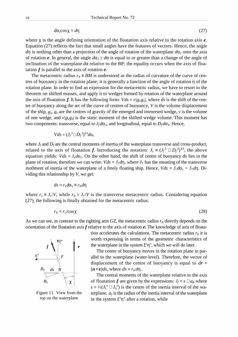
The central moments of the waterplane relative to the axis of floatation f are given by the expressions: Jf = s + af, where s = ½(Jξ'' + Jη'') is the centre of the inertia interval of the wa-terplane, af is the radius of the inertia interval of the waterplane in the system ξ''η'' after a rotation, while
ef
B2
B1
B
χ
ds
F
ξ''
η''
Figure 11. View from the
top on the waterplane

Technical Report No. 72
19
Df = a''sin2χ + D''cos2χ af = a''cos2χ − D''sin2χ
(29)
a'' = ½(Jξ'' − Jη'') is the radius of the inertia interval before rotation (in the ξ''η'' system), whereas D'', Jξ'', Jη'' are the product, transverse and longitudinal moments of inertia of the waterplane in the central system ξ''η'', parallel to the axis of rotation e (Figure 11). The above expressions result from the transformation of the moments of inertia due to rotation of the central system ξ''η'' by an angle χ, given in the appendix.
Rotating the waterplane by an angle dα1, the transverse component of the buoyancy centre displacement BB1, relative to the axis of floatation (Figure 11) is proportional to Jf, whereas the longitudinal component B1B2 is proportional to Df. We want the resultant displacement to be normal to the direction of the heeling moment (axis of rotation e). To be so, the angle B in Figure 11 has to be equal to χ, which results from the property of angles, whose arms are re-spectively normal. Hence, the angle of inclination of the axis of floatation relative to the axis of rotation has to satisfy the equation:
tanχ = Df /Jf (30)
The angle χ has the same sign as that of the waterplane product of inertia (in Figure 11 it is posi-tive). It should be remembered that moments Df and Jf are also dependent on the angle χ, which converts the above formulation to an equation. Substituting Jf = s + af, equation (30) will take the form:
Df − (s + af) tanχ = 0
The quantities Df and af, given by equation (29), represent a parametric equation of the Mohr’s circle (Figure 12). Substituting them to the above equation yields:
rsin(2γ + 2χ) − [s + rcos(2γ + 2χ)] tanχ = 0 (31)
where r = (a2 + D2)1/2 is a radius of the Mohr’s circle, independent of the orientation of a central system, the phase 2γ0 = tan− 1(D''/a''), the angle 2γ = 2γ0, if a'' > 0, otherwise 2γ = 2γ0 + 180º. Equation (30), with the use of the quantities D'' and a'', is easier to solve, whereas equation (31) is easier for geometrical interpretation (Figure 12); a'' and γ0 are negative in this figure.
Figure 12. Mohr’s circle for the waterplane
Technical Report No. 72
20
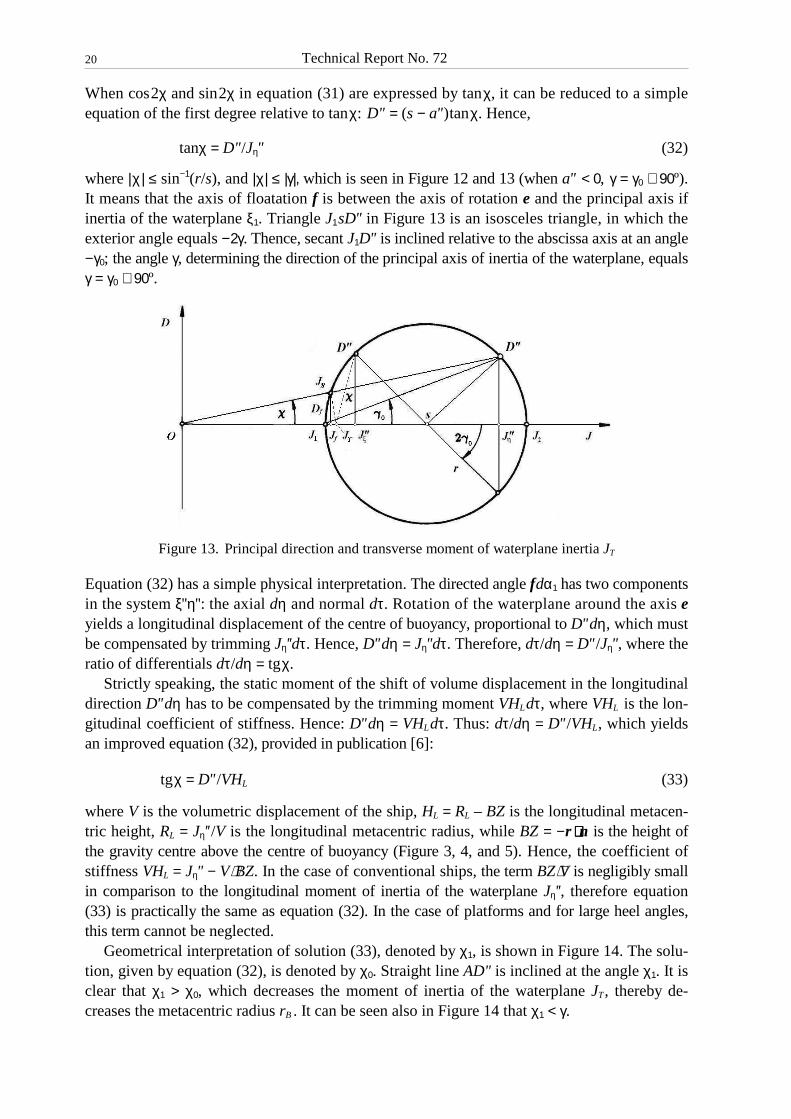
When cos2χ and sin2χ in equation (31) are expressed by tanχ, it can be reduced to a simple equation of the first degree relative to tanχ: D'' = (s − a'')tanχ. Hence,
tanχ = D'' /Jη'' (32)
where |χ| ≤ sin−1(r/s), and |χ| ≤ |γ|, which is seen in Figure 12 and 13 (when a'' < 0, γ = γ0 + 90º). It means that the axis of floatation f is between the axis of rotation e and the principal axis if inertia of the waterplane ξ1. Triangle J1sD'' in Figure 13 is an isosceles triangle, in which the exterior angle equals −2γ. Thence, secant J1D'' is inclined relative to the abscissa axis at an angle −γ0; the angle γ, determining the direction of the principal axis of inertia of the waterplane, equals γ = γ0 + 90º.
Figure 13. Principal direction and transverse moment of waterplane inertia JT
Equation (32) has a simple physical interpretation. The directed angle fdα1 has two components in the system ξ''η'': the axial dη and normal dτ. Rotation of the waterplane around the axis e yields a longitudinal displacement of the centre of buoyancy, proportional to D''dη, which must be compensated by trimming Jη''dτ. Hence, D''dη = Jη''dτ. Therefore, dτ/dη = D'' /Jη'', where the ratio of differentials dτ/dη = tgχ.
Strictly speaking, the static moment of the shift of volume displacement in the longitudinal direction D''dη has to be compensated by the trimming moment VHLdτ, where VHL is the lon-gitudinal coefficient of stiffness. Hence: D''dη = VHLdτ. Thus: dτ/dη = D'' /VHL, which yields an improved equation (32), provided in publication [6]:
tgχ = D'' /VHL (33)
where V is the volumetric displacement of the ship, HL = RL – BZ is the longitudinal metacen-tric height, RL = Jη'' /V is the longitudinal metacentric radius, while BZ = −r ⋅⋅⋅⋅ n is the height of the gravity centre above the centre of buoyancy (Figure 3, 4, and 5). Hence, the coefficient of stiffness VHL = Jη'' − V⋅ BZ. In the case of conventional ships, the term BZ⋅V is negligibly small in comparison to the longitudinal moment of inertia of the waterplane Jη'', therefore equation (33) is practically the same as equation (32). In the case of platforms and for large heel angles, this term cannot be neglected.
Geometrical interpretation of solution (33), denoted by χ1, is shown in Figure 14. The solu-tion, given by equation (32), is denoted by χ0. Straight line AD'' is inclined at the angle χ1. It is clear that χ1 > χ0, which decreases the moment of inertia of the waterplane JT, thereby de-creases the metacentric radius rB . It can be seen also in Figure 14 that χ1 < γ.

Technical Report No. 72
21
Figure 14. Mohr’s circle and stability characteristics
The knowledge of the angle χ defines the direction of the axis of floatation f. The unit vector of this axis is as follows:
f = ecosχ + (n × e)sinχ (34)
The transverse moment of inertia of the waterplane JT defines in turn the metacentric radius rB ≡ JT/V. Multiplying equation (28) by the volumetric displacement V, and accounting for equa-tion (30), the following is obtained:
JT = Js/cosχ = (Jf2 + Df
2)1/2/cosχ = Jf [1+ (Df /Jf )2]1/2/cosχ = Jf (1+ tg2χ)1/2/cosχ = Jf /cos2χ
Substituting Jf = s + af , where s = ½(Jξ'' + Jη'') is the centre of the inertia interval of the water-plane, while af is the radius of the inertia interval of the waterplane in the system ξ''η'' after a ro-tation by an angle χ, given by equation (29), the following is obtained:
JT = (s + af)/cos2χ = (s + a''cos2χ − D''sin2χ)/cos2χ = s/cos2χ + a''(2 – 1/cos2χ) − 2D'' tgχ = (s − a'')(1 + tg2χ) + 2a'' − 2D'' tgχ = s + a'' + (s − a'')tg2χ − 2D'' tgχ = Jξ'' + Jη'' tg2χ − 2D'' tgχ
Accounting equation (32), we get the equation:
JT = Jξ'' − D'' tgχ (35)
from which it follows that JT ≤ Jξ''. It means that balancing the ship decreases the transverse moment of inertia of the waterplane JT, and also the metacentric radius rB, which in turn causes a reduction of the righting arm – a conclusion consistent with the foregoing considerations that balancing the ship decreases the stability. The expression JT = Js/cosχ = Jξ'' − D'' tgχ has a simple interpretation, shown in Figure 13.
The above equation can be obtained directly. A rotation of the waterplane around the axis e yields a transverse shift of the centre of buoyancy, proportional to Jξ''dη. On the other hand, balancing the ship decreases this shift by D''dτ. The resultant shift, by definition, is propor-tional to JTdη. Hence: JTdη = Jξ''dη − D''dτ. Dividing it by dη it yields equation (35).
Equations (30), (32) and (33) were derived assuming that e ⋅ dr = 0, i.e. that the displacement of the centre of buoyancy dr is strictly perpendicular to the axis of rotation e. However, for a freely floating ship this is not the case. Note that when the ship is heeled the trim has to be changed to balance the ship, which changes orientation of the rotation axis e relative to the ship.

Technical Report No. 72
22
Differentiating the equation e ⋅ r = 0 we get: e ⋅ dr = −de ⋅ r, i.e. in the co-ordinate system fixed to the ship the displacement of the centre of buoyancy is not strictly normal to the axis of rota-tion. It should be intuitively obvious: since the centre of buoyancy has to remain all the time in the plane of rotation, which changes its orientation relative to the inclining ship, the displace-ment of the centre of buoyancy has to be oblique to it.
When the axis of floatation f is known, it is easy to find new analytical angles ϕ and θ, de-scribing orientation of the ship relative to the water at the new angle of heel. Namely, rotating the waterplane by an angle ∆α1, the unit vector n rotates around the axis of floatation by the angle ∆α1. Hence, the new unit vector n1 is as follows:
n1 = ncos∆α1 + (f × n)sin∆α1 (36)
Knowing new unit vector n (≡ n1), the new analytical angles, corresponding to the new unit vector can be easily obtained from equation (3). Namely, tanθ = −nx/nz, whereas tanϕ = −ny/nz. The knowledge of new angles of waterplane inclination largely speeds up the process of find-ing the correct location of the centre of buoyancy at a new angle of heel ϕ, φ or α, depending on the line of nodes. The equation of new waterplane at first iteration is as follows:
nx(x − xF) − ny(y − yF) − nz(z − zF) = 0 (37)
where xF, yF, zF are co-ordinates of the previous centre of floatation F, whereas (nx, ny, nz) = n1 are components of the new unit vector n. Equation (37) is more convenient than equation (1), as with an increase of heel tanϕ and T0 grow indefinitely. Equation (1) is essential to start the calculations. Knowing equation of the waterplane it is necessary to check by iterations, if the ship displacement V = const is conserved, and if the ship is longitudinally balanced, i.e. if the equation e ⋅ r = 0 is satisfied. If not, then the waterplane should be shifted in the normal direc-tion by a distance ∆n = −∆V/AWL, and the trim angle Θ, θ or ϑ, depending on the line of nodes, should be corrected accordingly. If the centre of buoyancy is in front of the plane of rotation (le > 0), the trim angle should be somewhat decreased, by rotating the waterplane around the axis η'' (Figure 11) in positive direction by an angle ∆τ = le/HL, where HL is the longitudinal metacentric height. This reasoning is fully correct for the reference axis Ox', where the axis η'' is parallel to the trace of water in vertical frame sections (Figure 3). In the case of other reference axes, the ship has to be rotated around a normal to the PS (Figure 4) or to the ini-tial waterplane (Figure 5) to avoid a change of the heel angle. Depending on the line of nodes, the vertical change of the trim angle is as follows:
−∆τ = ∆Θ = ∆θcosφ = −∆ϑsinα (38)
which results from the vector properties of small rotations, i.e., a projection of the directed angle of trim on the horizontal plane (Figure 15). Substituting ∆τ = le/HL, the following is obtained:
∇φ
jdθPS
∇
−−−−kdϑ
α
Figure 15. Positive change of oblique trim

Technical Report No. 72
23
−le = HL∆Θ = (HLcosφ)∆θ = −(HLsinα)∆ϑ
The multipliers of the trim changes are the coefficients of stiffness with respect to trim, i.e., the longitudinal metacentric heights. Except the vertical trim, in the case of oblique trims the metacentric heights are incomplete, as they neglect the effect of the vertical change of trim, which turns the ship in the horizontal plane. Calculations of the GZ-curve can be significantly accelerated, if they are based on the Kryłov–Dargnies' method, modified for a freely floating ship, utilising the properties of equi-volume waterplanes for such a ship, unknown in literature. In a finite interval of the angle of rotation ∆η equi-volume waterplanes roll over the surface of a certain cone, the parameters of which can be predicted in advance [6]. The rolling waterplanes are tangent to the cone along the instantaneous axis of floatation f.
4.5. Mechanism of equi-volume inclinations
An infinitesimal rotation of the waterplane around the axis of floatation f can be regarded as resulting from two rotations: ship's rotation by an angle dη around the axis ξ'', parallel to the axis of rotation e, and ship's rotation by angle dτ around the axis η'', normal to the axis of rota-tion e (Figure 11). Hence, the directed angle fdα1 has two components in the system ξ''η'', equal to the two said elementary rotations: fdα1 = (dη, dτ).
The directed angle fdα1 is inclined at an angle χ to the rotation axis e (Figure 11). Positive angle χ corresponds to positive normal component of dτ, whereas the change of trim is negative (by stern), therefore the normal component has to be taken with an opposite sign. Projection of dα1 on the rotation axis yields equation (27). Resorting to the relationships inherent for rectangu-lar triangles, normal component of dτ can be written in two ways:
dτ = dα1sinχ = dη tanχ (39)
The above equation indicates that: 1° the more deflected the floatation axis from the rotation axis, the greater changes of ship trim during inclinations, which is intuitive; 2° when χ = 0, i.e. when e = f, the ship trim does not change, as for a ship with fixed trim; 3° from equation (38) it follows that for φ = 90° (the PS is then horizontal) dτ = 0. We will see later that it is im-possible for a free floating ship to achieve the angle φ = 90°.
In the case of the reference axes y and z, the rotation of the reference planes around normal vectors, associated with trimming, equals to jdθ or −kdϑ has also a vertical component dψ, which equals the rotation (the change of orientation) of the ship in the sea surface. In the case of PS, it equals dθsinφ, and in the case of BP, it equals −dϑcosα (Figure 15); note that in the said figures the heel angle is negative. Hence,
dψ = −dθ sinφ = −dϑcosα (40)
In both cases, the vertical component of rotation of the plane of rotation is directed down-wards, which means that rotation of the ship in the horizontal is clockwise. If this rotation was neglected, the trim would change the azimuth.
Considering equations (38) and (39) the differential dψ can be expressed in terms of an in-crease of the heel angle dη. Namely, dψ = dτ tanφ = dτcotα, where dτ = dη tanχ is a rotation of the ship in the horizontal. The angles of rotations of the PS or the initial waterplane around the trace of water have no vertical components, as they are directed horizontally (Figure 2).
A different situation occurs in the case of the reference axis x: a change of the trim angle, as a vector, is directed horizontally, therefore it has no vertical component (Figure 3). However, the
Technical Report No. 72
24
angle of rotation of the midships section around its normal −idϕ has a horizontal component: −dϕcosΘ, and vertical: −dϕsinΘ. Rotations of the waterplane relative to the ship have the oppo-site sign: (dϕcosΘ, dϕsinΘ). The horizontal component is the angle of rotation of the waterplane relative to the ship. Hence, dη = dϕcosΘ. The vertical component dψ = dϕsinΘ = dηtanΘ is a change of orientation of the rotation axis e relative to the ship. When in an upright position the ship is trimmed, the angles ϕ and Θ are replaced by ϕ' i Θ', and the angles α and ϑ by α' and ϑ'.
It is worth emphasising that the rotation of the ship in the horizontal by an angle dψ, induced by trimming (balancing) the ship, has no direct effect on calculating the GZ-curve. In particular, it has no effect on the orientation of the axis of floatation f in the ship system. Hence, if for a new waterplane the angle χ changes by dχ the new floatation axis will rotate relative the previous one by an angle dχ, as rotation of the ship in the horizontal plane does not change the waterplane. When the angle dχ > 0 is positive, the new floatation axis f shifts towards the heel, i.e. it departs from the rotation axis e.
Equi-volume waterplanes roll over a non-circular cone whose axis is inclined relative to the waterplanes by an angle ε determined by the following expression: sinε = dχ/dα1. The derivation of this equation is elementary. When a cone rolls over a plane with no slip, the base of the cone moves along an arc of length lχ = rα. Hence, χ/α = r/l = sinε, where χ is the angle of rotation of the cone in the plane, α is the angle of rotation of the cone around its own axis of symmetry, r is the radius of the base, and l is the length of the generatrix. In kinematics, the said cone, over which equi-volume waterplanes roll over, is an example of a ruled fixed axode, whereas rolling waterplanes – of a moving axode.
When the angle dχ > 0 is positive the cone is located above the waterplanes, if not – below. The apex of the cone is located at a distance from the generatrix l from the centre of floatation F, given by the equation l = −dη'F/dχ, where dη'F is the displacement of the centre of floata-tion normal to the axis floatation (when l > 0, the apex is located in the direction of the bow). Taking into account that dη'F = rFdα1 one obtains:
l = −rF dα1/dχ = −rF/sinε
where rF = dJf /dV is a differential metacentric radius (radius of curvature of the curve of centres of floatation). This formulation shows that the radius of the cone base at the level of the centre of floatation is equal to the differential metacentric radius.
EXAMPLE. It can be shown that the angle between two waterplanes is given by the equation:
cosα' = cos2εcosα + sin2ε
Commonly, the angle ε ≈ 0 is small, then α' ≈ α.
If ship heel is increased by dη, the displacement of the centre of buoyancy, normal to the plane of rotation, is proportional to D''dη, where D'' is the product of inertia of the waterplane in the ξ''η'' system (Figure 11). The said displacement must be compensated by trim Jη''dτ. Equating them to each other one gets dτ = (D''/Jη'')dη. Hence, dτ/dη = D''/Jη''. Taking into account equation (39), the above yields equation (32). A more exact solution can be obtained by using the metacentric formulation for dτ = (D''/VH0)dη, where H0 ≡ GML = BML − BZ is the longitudinal metacentric height. As tanχ = dτ/dη, the above yields equation (33), recalled before without derivation.
The righting arm of the ship is given by equation (22). In order to make use of it, for given heel angle η = const and given volume displacement V = const we have to know the trim at which the ship is balanced, i.e. e ⋅ r = 0. Usually, we find it by an iterative method. This process can be accelerated, if the change of the longitudinal component of the righting arm dle = d(e ⋅ r) = de ⋅ r + e ⋅ dr, induced by trim is known.

Technical Report No. 72
25
The change of the axis of rotation de in the ship hull system induced by trimming can be easily worked out with the help of Figure 3, Figure 4, and Figure 5. In the first case the change results from vertical rotation of the unit vector e by an angle dΘ, in the second – by an angle dθ in the PS, and in the third case – by an angle dϑ in the initial waterplane. Hence,
de = ndΘ de = (e × j)dθ de = −(e × k)dϑ
(41)
Thus, de ⋅ r = r ⋅⋅⋅⋅ ndΘ = −BZdΘ de ⋅ r = r ⋅⋅⋅⋅ (e × j)dθ = r ⋅⋅⋅⋅ eZ = rZdθ = −(BZcosφ − lsinφ)dθ de ⋅ r = −r ⋅⋅⋅⋅ (e × k)dϑ = r ⋅⋅⋅⋅(k × e)dϑ = (BZsinα + lcosα)dϑ
where BZ is a vertical distance between the ship centre of gravity and centre of buoyancy (Figure 3), eZ ≡ e × j is the unit vector of the OZ axis, fixed to the plane of rotation; the said axis is the edge of intersection between the PS and rotation plane (Figure 4), rZ is a projection on the axis OZ of the radius vector r of the centre of buoyancy relative to the ship centre of gravity, and r ⋅⋅⋅⋅ (k × e) is a projection of r on the edge of intersection between the plane of rotation and the initial waterplane. The second relation results from a projection of the segment BZ on the OZ-axis, deviated from the vertical by the angle φ (Figure 4), and the third one – from a projec-tion of BZ on the axis Oz', deviated from the vertical by the angle α' (Figure 5).
In the case of the reference axis Ox', the second contribution to the change dle is given by the relation: e ⋅ dr = RLdΘ, where RL is the longitudinal metacentric radius, which follows from the preceding considerations. For other reference axes, the vertical change of the trim angle is given by equation (38).
In addition, we have to account for the effect of rotation of the ship in the horizontal on the displacement of the centre of buoyancy relative to the (stationary) plane of rotation. It equals −ldψ, which directly results from Figure 4 and Figure 5, where dψ is the trim induced rotation of the ship in the horizontal, given by equation (40), and l ≡ GZ is the righting arm. When dψ < 0 is negative, the rotation is clockwise, while the displacement of the centre of buoyancy is positive, i.e. in bow direction. For the reference axis x', dψ = 0, since the vertical change of trim does not cause any rotation in the sea surface (Figure 3); the said rotation occurs only during oblique trimming (see Figure 4 and Figure 5).
Hence, combining the said contributions, depending on the reference axis the following is obtained for change of the trimming arm dle:
dle = (RL − BZ)dΘ dle = [RLcosφ − (BZcosφ − lsinφ) + lsinφ] dθ dle = [−RLsinα + (HFsinα + lcosα) + lcosα] dϑ
After simplifications, we get finally:
dle = HLdΘ dle = (HLcosφ + 2lsinφ)dθ dle = (HLsinα − 2lcosα)(−+dϑ)
(42)
In the third case, we have to pay attention to the sign of α. When the heel is to portside (α > 0), a positive increase of the twist angle dϑ means trimming by aft, i.e. the change dle < 0 is nega-tive. Hence, dϑ has to be taken with the opposite sign. When the heel is to starboard (α < 0),
Technical Report No. 72
26
a positive increase of the twist angle dϑ produces the change dle consistent with the sign of dϑ. In other words, the expression for HLϑ changes the sign when α < 0.
These equations allow for a quick finding of the equilibrium trim. The expressions in the parentheses represent a derivative of the longitudinal component of the righting arm le relative to the respective trim angle, that is, the longitudinal metacentric height for a given reference axis HLΘ HLθ i HLϑ, understood as the stiffness relative to a respective trim angle. The first one is the classic longitudinal metacentric height HLΘ ≡ HL for vertical trims. In the case of oblique trims, the longitudinal metacentric height depends additionally on the righting arm l ≡ GZ.
In the course of heeling the longitudinal metacentric height varies. When it becomes negative, it means the lack of longitudinal balance, ipso facto, the lack of opportunity for determining the righting arm. This phenomenon is termed as fading stability. This phenomenon does not occur when doing calculations with fixed trim – the GZ-curve is defined at each heel angle.
In an upright position HLΘ = HLθ = HL, and HLϑ = −2l0. When l0 = 0, where l0 is the righting arm in an upright position, the longitudinal metacentric height is an even function of the heel angle. When l0 ≠ 0, i.e., when an initial heel occur, in the case of the reference axis Oz' the GZ-curve is indefinite in some one-sided neighborhood of zero. For two other reference axes, the GZ-curve is continuous around zero. When α→90°, HLϑ→HL tends to the longitudinal metacen-tric height, as for the reference axis Ox', whereas HLθ tends to negative values. It means that in some vicinity of the angle φ = 90° the GZ-curve related to the reference axis Oy is indefinite.
The expression for HLϑ allows for the estimation of the external end of the interval, in which the GZ-curve for the axis Oz' is indefinite. From equation (42) the following results:
tanα = 2l/HL (43)
The above angle can be expressed in terms of the initial heel α0. Assuming that α0 = −l0/h0, where h0 is the initial metacentric height, we get: α = −2α0h0/HL. As we can see, the length of the interval with faded stability is proportional to the angle of initial heel, located on the other side of zero, starting exactly at zero. For conventional ships the said interval is imperceptible. However, it is characteristic for semisubmersible platforms, particularly for jack-up rigs, where the longitudinal metacentric height is relatively small and the righting arms relatively large. For inclinations in the direction of the initial heel, the GZ-curve is definite at each point.
The angle χ, given by equation (33), describing orientation of the axis of floatation f rela-tive to the axis of rotation e, was obtained without accounting of the rotation of the ship in the horizontal plane. The said angle affects the transverse metacentric radius rF = JT/V through the transverse moment of inertia of the waterplane JT, given by equation (35). The improvement of the relation for the angle χ is simple. The rotation of the ship by an angle dη yields not only the static moment of shifting the displacement in the longitudinal direction, equal to D''dη, but yields also the rotation in the horizontal by an angle dψ = dϕsinΘ, directed upwards, if the ship is trimmed by bow. The said rotation moves the centre of buoyancy away from the plane of rotation towards the aft by ldψ. The resultant change of the static moment has to be com-pensated by a trimming moment VHLdτ. Hence:
D''dη – Vldψ = VHLdτ, D'' – Vldψ/dη = VHLdτ/dη.
Accounting that dψ/dη = tgΘ, and dτ/dη = tgχ, the following is obtained:
tgχ = (D'' − VltgΘ)/VHL (44)

Technical Report No. 72
27
The above equation is valid for the reference axis Ox. When the ship has an initial trim, the angle Θ is replaced by Θ'. If tanΘ is negligible, the above reduces to equation (33).
In the case of the two remaining reference axes, the elementary rotation of the ship dη, equal to dφ or dα, there is no a vertical component. Therefore, the static moment of shifting the displacement in the longitudinal direction D''dη has to compensated by trimming –Vdle, where dle is given by equation (42). Hence: D''dη has to be equal to –VHLθdθ or VHLϑdϑ. Ac-counting for equations (38), the following is obtained:
tgχ = cosφD'' /VHLθ tgχ = –sinαD'' /VHLϑ
(45)
When the ship has an initial trim, the angle a is replaced by α'.
4.6. Properties of the GZ-curve
Knowing metacentric radii for a freely floating ship one can easily find the remaining proper-ties of the GZ-curve. They are analogous to those known from the classic ship theory. Like so, the metacentric height h ≡ ZM is equal to:
h = d/dη l = rB − BZ (46)
where rB ≡ BM is the metacentric radius, given by equation (28), BZ = −r ⋅⋅⋅⋅ n is the height of ship centre of gravity above the centre of buoyancy (Figure 3, 4 and 5), r = GB is the radius-vector of ship centre of buoyancy relative to its centre of gravity, and n is a unit vector normal to the waterplane, as given by equation (3), or alternative ones. Equation (46) can be immedi-ately obtained by considering the line of action of buoyancy in the plane of rotation (Figure 16) for heel angle increased by dη, where the angle of rotation η = φ or α, depending on the line of nodes (the system B0YZ is fixed to the plane of rotation, whose origin is at an initial position of the centre of buoyancy B0). The metacentric height can be also obtained by differentiating the
righting arm l ≡ GZ, given by equation (22), with respect to heel angle (angle of rotation) in the ship-fixed refer-ence system. This derivative is given by:
GZ' = e'⋅ (r × n) ++++ e ⋅ (r ' × n) ++++ e ⋅ (r × n' ) = rB + r ⋅⋅⋅⋅n
identical with equation (46), where the sign ' stands for differentiating respective to the heel angle η. It can be dem-onstrated that the first term e'⋅ (r × n) vanishes (it is suffi-cient to observe that the three vectors are coplanar, i.e. lie in the plane of rotation), the second one is the metacentric radius rB = BM, and the third one equals r ⋅⋅⋅⋅ n.
Work done by the righting moment M is given by the equation:
L = ∫0
ηMdη = D ∫0
ηldη = Dld
ld = ∫0
ηldη (47)
where D is buoyancy of the ship, and ld is the dynamic arm, the same as the first integral curve of the GZ-curve, i.e. the area under the GZ-curve. The dynamic arm is proportional to work done by the righting moment. Considering rotation of the plane of rotation by an angle dη (Figure 3–5, Figure 16), one can easily demonstrate that the differential GZdη = d(BZ) is an
Figure 16. Rotation plane
Technical Report No. 72
28
increment of the segment BZ due to the vertical shift of point Z, as the buoyancy centre B moves horizontally, i.e. parallel to the waterplane. Hence, the known formulation for the dy-namic arm is obtained:
ld = BZ − a (48)
where a = B0G is the height of the ship gravity centre G over buoyancy centre in an upright posi-tion (i.e. for η = 0). The said equation has a simple physical interpretation – the dynamic arm is equal to the vertical increment of the distance between the centre of gravity and centre of buoyancy. It can be useful in checking accuracy of calculation of the GZ-curve. The initial heel has no effect on this equation.
It is worth mentioning that the GZ-curve with free trim complies with the theorem of mini-mum potential energy, i.e. heeling of the ship (understood as rotation of the plane of rotation) by a given angle requires the least work. This is an important feature of the GZ-curve. The de-flection of the ship from its longitudinal equilibrium is not possible without applying a trimming moment and doing additional work that increases its potential energy, which proves the above theory. Thus, the GZ-curve with free trim is at most equal to or smaller than that of a ship with fixed trim, clearly illustrated in Figure 1. Otherwise, it means that the calculation algorithm is flawed.
Considering the above, the following holds for the dynamic arms of a freely floating ship and with fixed trim:
ld = ldc − ∫0
Θ(e ⋅ r)dΘ
where Θ is the trim angle for a given angle of rotation η of the plane of rotation, measured at a vertical plane. If one assumes that the longitudinal metacentric height HL is constant in the course of trimming, then equation (42) yields that (e ⋅ r) = HLΘ. Hence, ld ≈ ldc − ½HLΘ2. As can be seen the sign of the trim has no meaning. Differentiating this equation with respect to the angle of rotation η of the plane of rotation, we get l ≈ lc − ½(HLΘ2)'. Hence,
l ≈ lc − (½HL' Θ2 + HLΘΘ') (49)
From this equation two important conclusions can be drawn. Firstly, the greater the change of trim after balancing the ship, the lesser is the GZ-curve with free trim. Secondly, the GZ-curves of yet smaller arms would have to have yet larger trim changes, which is impossible due to the lack of other equilibrium trim than that for a freely floating ship. By changing the trim, the cen-tre of buoyancy permanently moves away from the plane of rotation. Hence, the GZ-curves with free trim are identical with the GZ-curves of minimum stability. In other words, the longitudinal balance of the ship provides at the same time the minimum potential energy at a given heel angle.
When the ship at the initial position has an initial trim Θ0 the angle of trim in equation (49) should be understood as change of trim Θ − Θ0. It is worth remembering that a fixed trim θ, measured in the PS, does not mean that trim at a vertical plane Θ = const. Equation (4) implies that when θ = const, the angle Θ decreases to zero, when ϕ tends to 90°. This means that with an increase of the heel angle the difference between the GZ-curves at level keel and with fixed trim as in the initial position, should vanish, supported also by numerical calculations.
4.7. Cross-curves of stability
The lever of hull form, i.e. the arm of buoyancy force relative to the initial location of centre of buoyancy, shown in Figure 16, is given as follows:

Technical Report No. 72
29
lB = GZ + asinη (50)
For a freely floating ship, which changes its trim during heeling, hull form arms depend on the height of centre of gravity over the BP. In the case of trim, while changing KG-value the centre of gravity does not remain in the original plane of rotation, which causes a change of ship trim, and entails in turn a change of hull form arm, thus making it dependent upon the KG-value. Hence, strictly speaking, the idea of cross curves of stability does not apply to a freely floating ship.
Note that the z-axis does not lie in the rotation plane, which is inclined to it at an angle δ, given by the equation: sinδ = e ⋅ k = ez. For the reference axis x, the rotation axis is given by equation (21). Hence, sinδ = cosϕtanθcosα = tanΘcosα. For the reference axis y, it is easy to obtain that the deviation δ = θ, and for the reference axis Oz', normal to the initial waterplane, δ = 0, i.e. the axis Oz' lies in the rotation plane.
Hence, shifting the centre of gravity along the z-axis by a quantity ∆zG causes point G to shift before the rotation plane by a distance le = ∆zGsinδ. As a result the ship becomes unbalanced and must trim in the vertical plane by an angle dΘ = le/HL, where HL is the longitudinal meta-centric height at given heel angle η. The ship is balanced by changing its trim angle, without changing its heel angle. In this case, the relationship between trim angles is such, as in equation (38). This defines the trim correction, depending on the reference axis. From Figure 16 it can be established that the new righting lever is equal to:
l1 = l − ∆zGcosδsinη + (D''/V) ∆Θ (51)
where D'' is the product of inertia of the waterplane in the system ξ''η'' (Figure 11). For common trims the function cosδ ≈ 1 can be omitted. Two first terms in the above equation are the same as for a ship with fixed trim. The last term (D''/V) ∆Θ, denoted further down by ∆l, accounts for the effect of trim change on the GZ-curve with free trim. Considering that ∆Θ = le/HL, and re-sorting to equation (33), one obtains:
∆l = ∆zGsinδtanχ (52)
The above correction vanishes for the reference axis Oz', as δ = 0. For other cases additional information is needed on the run of the angles δ and χ as function of heel angle η for calcula-tion of the correction ∆l. The said angles, however, depend on the position of centre of gravity of the ship, which makes the idea of cross-curves of stability invalid.
A way out of the situation is calculation of cross-curves of stability in the form of the GZ-curve for a typical location of the ship's centre of gravity. The correction ∆l is then small, and can be frequently neglected. For modest changes of the height of centre of gravity the ratio ∆l/∆zG = sinδ tanχ is practically independent of the position of the centre of gravity. For cal-culating the correction ∆l it is sufficient to know the run of the said ratio as a function of heel angle η. Equation (51) for a new GZ-curve takes then the form:
l1 = l − (sinη − sinδ tanχ)∆zG (53)
Cross-curves of stability are usually presented in the form of a graph: l = l(V, η = const). In a similar manner a graph of the ratio ∆l/∆zG = sinδtanχ should be presented, as a function of V, with heel angle η as a parameter.

Technical Report No. 72
30
5. KINEMATICS OF A FREELY FLOATING SHIP
The attitude (orientation) of the waterplane relative to the ship is described by the analytical angles ϕ and θ. All other angles between various planes and axes can be expressed using the two angles, where these relations do not depend on the reference axis. The choice of the ref-erence axis affects, however, orientation of the axis of floatation f on the waterplane, and the ship itself relative to the plane of rotation, in which it is balanced (large circle in Figure 3, Figure 4, Figure 5), and hence – the righting lever l ≡ GZ, given by equation (22).
For example, equation (3) for components of the unit vector n, normal to the waterplane, is valid regardless of the choice of the reference axis. In any case, it can be expressed directly with the help of the Euler’s angles, appropriate for a given reference axis. When the line of nodes is the trace of water in the BP (which applies, when at an upright position the ship is at level keel), the analytical angles in equation (3) have to be replaced by the Euler’s angles ϑ and α. Substi-tuting for tanθ = −sinϑtanα, and for tanϕ = cosϑtanα, the following is obtained:
n = (sinϑsinα, −cosϑsinα, cosα) (54)
The above is identical with equation (20). When in an upright position the ship is trimmed, the an-gles α and ϑ are replaced by α' and ϑ'. The line of nodes is then the trace of water on the initial waterplane, i.e. the edge of intersection between the initial and actual waterplanes.
When the line of nodes is the trace of water in the PS, the Euler’s angles are the angles θ and φ. Taking into account cosα = cosθcosφ and equation (5) on tanφ the following is obtained from equation (3):
n = (−sinθcosφ, −sinφ, cosθcosφ) (55)
Similarly, when the line of nodes is the trace of water in the midships section, the unit vector n can be expressed in terms of the Euler’s angles ϕ and Θ, as follows:
n = (−sinΘ, −cosΘsinϕ, cosΘcosϕ) (56)
When in an upright position the ship is trimmed, the angles ϕ and Θ are replaced by ϕ' and Θ'. In the case of the reference axis Ox', commonly used for calculating the GZ-curves with free
trim, e.g. in the NAPA software, PROTEUS, STATAW, WinSEA, and in many other computer programs, the plane of rotation is a vertical frame station, parallel to the trace of water in the frames (Figure 3); in the case of the axis Oy, it is normal to the trace of water in the PS (Figure 4), and in the case of the axis Oz', it is normal to the trace of water in the initial waterplane (Figure 5). In other words, in the first case the plane of rotation is parallel to the line of nodes, while in the two remaining cases it is normal to the line of nodes.
It is worth emphasising that in space there is only one rotation plane (large circle in the said figures). However, the ship sets differently with respect to it depending on the way of balancing. In the case of the reference axis Ox', longitudinal balance of the ship is achieved by vertical trim-ming around the trace of water in the vertical frame planes (Figure 3), in the case of the axis Oy – around a normal to the PS (Figure 4), i.e. around the y-axis, and in the case of the axis Oz' – around a normal to the initial waterplane (Figure 5). Hence, the ship after balancing has various orientations relative to the plane of rotation, producing different righting arms, dependent on the way the ship is balanced (the choice of the reference axis). Nonetheless, the direction of the righting moment in space is the same. The various orientations of the planes of rotation relative to the trace of water in the PS (the axis ξ) are illustrated in Figure 17. Deviations of these planes from a plane normal to the axis ξ, are described by the angles γ1, γ2 and γ3. Frequently, γ2 = 0, while
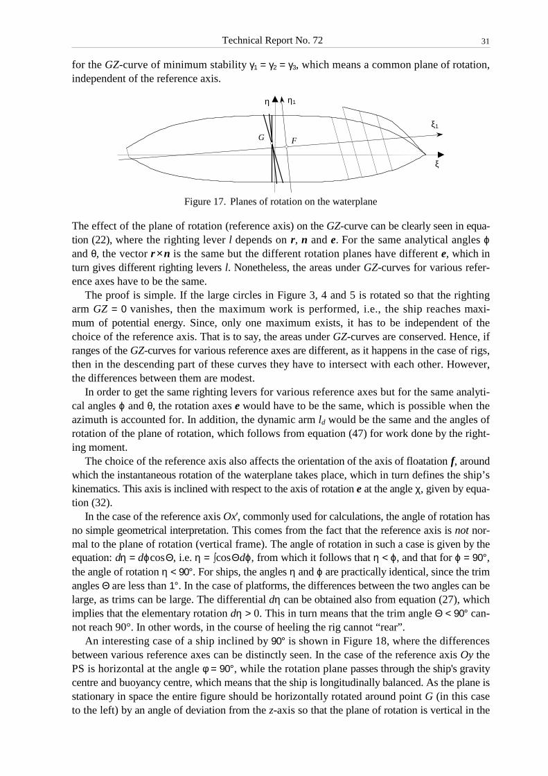
Technical Report No. 72
31
for the GZ-curve of minimum stability γ1 = γ2 = γ3, which means a common plane of rotation, independent of the reference axis.
ξ
η
G F
ξ1
η1
Figure 17. Planes of rotation on the waterplane
The effect of the plane of rotation (reference axis) on the GZ-curve can be clearly seen in equa-tion (22), where the righting lever l depends on r, n and e. For the same analytical angles ϕ and θ, the vector r × n is the same but the different rotation planes have different e, which in turn gives different righting levers l. Nonetheless, the areas under GZ-curves for various refer-ence axes have to be the same.
The proof is simple. If the large circles in Figure 3, 4 and 5 is rotated so that the righting arm GZ = 0 vanishes, then the maximum work is performed, i.e., the ship reaches maxi-mum of potential energy. Since, only one maximum exists, it has to be independent of the choice of the reference axis. That is to say, the areas under GZ-curves are conserved. Hence, if ranges of the GZ-curves for various reference axes are different, as it happens in the case of rigs, then in the descending part of these curves they have to intersect with each other. However, the differences between them are modest.
In order to get the same righting levers for various reference axes but for the same analyti-cal angles ϕ and θ, the rotation axes e would have to be the same, which is possible when the azimuth is accounted for. In addition, the dynamic arm ld would be the same and the angles of rotation of the plane of rotation, which follows from equation (47) for work done by the right-ing moment.
The choice of the reference axis also affects the orientation of the axis of floatation f, around which the instantaneous rotation of the waterplane takes place, which in turn defines the ship’s kinematics. This axis is inclined with respect to the axis of rotation e at the angle χ, given by equa-tion (32).
In the case of the reference axis Ox', commonly used for calculations, the angle of rotation has no simple geometrical interpretation. This comes from the fact that the reference axis is not nor-mal to the plane of rotation (vertical frame). The angle of rotation in such a case is given by the equation: dη = dϕcosΘ, i.e. η = ∫cosΘdϕ, from which it follows that η < ϕ, and that for ϕ = 90°, the angle of rotation η < 90°. For ships, the angles η and ϕ are practically identical, since the trim angles Θ are less than 1°. In the case of platforms, the differences between the two angles can be large, as trims can be large. The differential dη can be obtained also from equation (27), which implies that the elementary rotation dη > 0. This in turn means that the trim angle Θ < 90° can-not reach 90°. In other words, in the course of heeling the rig cannot “rear”.
An interesting case of a ship inclined by 90° is shown in Figure 18, where the differences between various reference axes can be distinctly seen. In the case of the reference axis Oy the PS is horizontal at the angle φ = 90°, while the rotation plane passes through the ship's gravity centre and buoyancy centre, which means that the ship is longitudinally balanced. As the plane is stationary in space the entire figure should be horizontally rotated around point G (in this case to the left) by an angle of deviation from the z-axis so that the plane of rotation is vertical in the
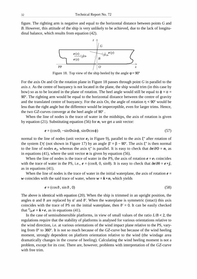
Technical Report No. 72
32
figure. The righting arm is negative and equal to the horizontal distance between points G and B. However, this attitude of the ship is very unlikely to be achieved, due to the lack of longitu-dinal balance, which results from equation (42).
G
x
z
OPP
e (z)
e (x) e (y)
B
Figure 18. Top view of the ship heeled by the angle φ = 90°
For the axis Ox and Oz the rotation plane in Figure 18 passes through point G in parallel to the axis z. As the centre of buoyancy is not located in the plane, the ship would trim (in this case by bow) so as to be located in the plane of rotation. The heel angle would still be equal to ϕ = α = 90°. The righting arm would be equal to the horizontal distance between the centre of gravity and the translated centre of buoyancy. For the axis Ox, the angle of rotation η < 90° would be less than the right angle but the difference would be imperceptible, even for larger trims. Hence, the two GZ-curves converge at the heel angle of 90° .
When the line of nodes is the trace of water in the midships, the axis of rotation is given by equation (21). Substituting equation (56) for n, we get a unit vector:
e = (cosΘ, −sinΘsinϕ, sinΘcosϕ) (57)
normal to the line of nodes (unit vector e2 in Figure 9), parallel to the axis ξ'' after rotation of the system ξ'η' (not shown in Figure 17) by an angle β' = β − 90°. The axis ξ'' is then normal to the line of nodes e2, whereas the axis η'' is parallel. It is easy to check that ∂e/∂Θ = n, as in equations (41), where the unit vector n is given by equation (56).
When the line of nodes is the trace of water in the PS, the axis of rotation e = e1 coincides with the trace of water in the PS, i.e., e = (cosθ, 0, sinθ). It is easy to check that ∂e/∂θ = e × j, as in equations (41).
When the line of nodes is the trace of water in the initial waterplane, the axis of rotation e = w coincides with the said trace of water, where w = k × n, which yields
e = (cosϑ, sinϑ , 0) (58)
The above is identical with equation (20). When the ship is trimmed in an upright position, the angles α and ϑ are replaced by α' and ϑ'. When the waterplane is symmetric (intact) this axis coincides with the trace of PS on the initial waterplane, then ϑ' = 0. It can be easily checked that ∂/∂ϑe = k × e, as in equations (41).
In the case of semisubmersible platforms, in view of small values of the ratio L/B < 2, the regulations require that the stability of platforms is analysed for various orientations relative to the wind direction, i.e. at various orientations of the wind impact plane relative to the PS, vary-ing from 0° to 360°. It is not so much because of the GZ-curve but because of the wind heeling moment, strongly dependent on platform orientation relative to the wind (the windage area dramatically changes in the course of heeling). Calculating the wind heeling moment is not a problem, except for its cost. There are, however, problems with interpretation of the GZ-curve with free trim.

Technical Report No. 72
33
Equations (18) and (19) imply that transverse l and longitudinal le components of the righting arm are functions of the angle of heel α' and angle of twist Ψ = ψ + ϑ'. The twist Ψ = Ψ(α') is a function of the angle of heel, which results from the longitudinal equilibrium, i.e. from the solution of the equation le(α', Ψ) = 0.
-3
-2
-1
0
1
2
3
4
5
0 45 90 135 180 225 270 315 360
α' = 11°
Ψ [°]
l = GZ
le = e⋅r
[m]
3ld
Figure 19. Run of transverse and longitudinal components of the righting arm l
and dynamic arm ld for rig II versus twist angle Ψ for a given heel angle
A graph of the function of two variables le = le(α', Ψ) is a surface. Curves, which result from the intersection of this surface with the plane le = 0 are a solution for the function Ψ = Ψ(α'). Hence, for a given heel angle α' = const there can only be a discrete number of twist angles Ψ at which a platform is in longitudinal balance. These angles can be easily found with the help of a graph le = le(α', Ψ) for a given heel angle α', as in Figure 19, carried out for platform II, investigated in chapter 7. As can be seen, for a given heel angle α' = 11° there are four twist angles Ψ, corre-sponding alternately to minimum and maximum stability. The first angle corresponds to the absolute minimum of stability, while the last one, to the absolute maximum. In any case, the first and third root is symmetric relative to the angle 90°, which can be proved strictly. These four equilibrium angles indicate that for a freely floating object only two meaningful orientations of the rotation axis e are possible, i.e. when it is parallel in an upright position to one or the other principal axis of inertia of the initial waterplane. The first orientation is the worst, i.e. it yields the GZ-curve of the lowest arms. When the waterplane is asymmetric, the ship has to be inclined towards the initial heel. In the second orientation there are unstable inclinations of maximum potential energy. At other orientations there are heel intervals, at which the unit cannot be longitudinally balanced. The GZ-curie is then indefinite.
Meanwhile, the regulations require the stability of platforms to be analysed at various orienta-tions relative to the wind direction, described by the azimuth ψ ∈ ⟨0°, 360°⟩, varying at every 5°. The azimuth is measured relative to the axis of rotation e, perpendicular to the wind direc-tion. Except for the four said orientations, i.e. ψ = 0°, 90°, 180° and 270°, in the remaining cases, if the ship is to be longitudinally balanced the GZ-curves for the reference axis Oz' are simply the same as for the azimuth ψ = 0, and for the other reference axes, the righting arms increase, assuming maximum values for the azimuth ψ = 90° and 270°, at the cost of increasingly extend-ing intervals in which the ship cannot be longitudinally balanced (Figure 20). The said figure, identical for the reference axes Ox'' and Oy', illustrate at the same time the effect of azimuth on the righting arm l ≡ GZ and dynamic arm ld for a fixed value of the heel angle α' = 11°. It is

Technical Report No. 72
34
worth noting that minima of the dynamic arm ld have the same values and occur at the same azimuth, irrespective of the reference axis.
-1
0
1
2
3
4
0 45 90 135 180 225 270 315 360
GZ
GZ
GZ
[m]
ψ [°]
α' = 11°
5ld
5ld 5ld
le le
Figure 20. Run of the righting arm l and dynamic arm ld for rig II
versus azimuth Ψ for a given heel angle
Nonetheless, as prompted by regulations, the GZ-curves are calculated for any orientations. This is possible only, when the platform is longitudinally unbalanced or wrongly balanced. If the ratio L/B is too small, the lack of longitudinal balance can occur also for inclinations around the longitudinal axis, which makes it impossible to find the GZ-curve. The lack of balance does not mean, however, that the platform then rears, as ABS publications claim [23, 24]. This phenome-non itself is termed there as orthogonal tipping. It is said that stability is then fading, in contrast to vanishing stability. The maximum trim in terms of absolute values depends on a given heel angle and does not generally exceed a dozen or so degrees. For example, for platform II, for the heel angle α' = 6° the angle θ > −9,83°, and for α' = 11° the angle θ > −15,21°. Orthogonal tipping does not take place in reality, which becomes self-explanatory in the light of the Krilov–Dargnies method.
6. GZ-CURVE OF MINIMUM STABILITY
As previously mentioned, most heeling moments acting on the ship, including the wind heeling moment, are parallel to the PS, therefore a free-floating ship assumes the position in which the trace of water in the PS is normal to the rotation plane. In the case of platforms arbitrarily ori-entated to the wind, the wind generated heeling moment is parallel to the wind impact plane, perpendicular to the wind direction in an upright position, fixed to the platform. Hence, the heeling moment is parallel to the trace of water in the impact plane, whereas the rotation plane is perpendicular to the said trace. A question then arises which position does the ship assume when the direction of the moment is not related to the ship?
In order to answer unequivocally this question, the mechanism of inclining the ship in the case of a free heeling moment must be known, as e.g. the one resulting from shifting a weight on board, or loading a weight at any place on the ship. In such a case the ship assumes a position in which the potential energy is minimal, i.e., the work required to incline the ship is the lowest. This property has a freely floating ship, longitudinally balanced. For a given heel angle there is only one equilibrium position e ⋅ r = 0, corresponding to minimum energy, independent of the reference axis.

Technical Report No. 72
35
The work is proportional to the dynamic arm, hence the minimum of potential energy cor-responds to the minimum of the dynamic arm ld, given by equation (48), valid in any case. From the classic ship theory it is known that the dynamic arm depends on the run of metacentric radii in function of the heel angle, which for a freely floating ship means in function of the rotation angle η of the rotation plane. Hence, in a general case:
ld = ∫0
ηrBsin(η − ν)dν − a(1 − cosη) (59)
where ν is a dumb variable of integration, varying from 0 to η (given angle of rotation of the rotation plane), rB is the metacentric radius in the rotation plane, given by equation (28), whereas
a = B0G is a constant, equal to the distance between the centre of buoyancy and centre of gravity at an upright position. It is obvious that the minimum is dependent on the first integral term in equation (59), which is mini-mal for the least metacentric radii in function of the rotation angle η. And this happens, when the angle χ by which the axis of floatation f is deviated from the axis of rotation e, given by equation (44) or (45), is minimal. This happens, when the azimuth ψ = 0, and when the ship is longitudinally balanced.
In other words, the ship inclines around the instan-taneous axis of floatation f. That is, it rolls over a non-circular cone (a fixed axode), tangent to the waterplane along a generatrix, coinciding with the axis of floata-
tion. The centre of buoyancy B moves in the ship system along a spatial curve, lying on the surface of a horizontal cylinder of varying radius of curvature, forming a kind of a helix, in-tersecting at a certain angle the stationary rotation plane (the large circle in Figure 3–5). At each point the said line has a tangent, parallel to the respective waterplane and normal to the axis of floatation (Figure 21). The righting arm l ≡ GZ is a chord of the arc, created by the pro-jection of the curve of centres of buoyancy on the sea surface, the axis of rotation e is per-pendicular to the righting lever l, inclined at an angle χ with respect to the axis of floatation f, while the dynamic arm ld is an increase of the vertical distance between points G and B.
The righting arm l ≡ GZ lies at the vertical rotation plane, stationary in space, passing through points G and B. The centre of buoyancy moves in the rotation plane along a flat curve of centres of buoyancy, whose metacentric radius rB = JT/V, where JT is the transverse moment of iner-tia of the waterplane, given by equation (35), dependent on the waterplane geometrical charac-teristics in the system related to the axis of rotation e.
The least GZ-curve, termed the GZ-curve of minimum stability is identical with the curve for a freely floating ship, related to the axis Oz'. The righting arm for a given heel angle corre-sponds to the first zero of the curve le ≡ e ⋅ r in function of the azimuth ψ (Figure 19). In this point the absolute minimum of potential energy occurs (minimum of the dynamic arm ld), clearly seen in the said figure, consistent with the meaning of this curve. The axis of floatation f is located between the axis of rotation e and the principal axis of inertia of the waterplane ξ1, as discussed in section 4.4.
GZ-curves for the reference axes Ox', Oy have the least values for the azimuth ψ = 0. They have the same area between the angle of equilibrium and angle of vanishing stability, as in the case of the axis Oz'. Therefore, they can also be regarded as the curves of minimum stability. The direction of the righting moment for the said reference axes, described by the axis of rota-
G
B
ξ1
l
d
f
c
e
Z
F
χ
Figure 21. Projection of curve of cen-
tres of buoyancy on the waterplane

Technical Report No. 72
36
tion e, is stationary in space. The same applies to the reference axis Oz', though it is said litera-ture that the righting moment of the curve of minimum stability has a varying direction in space, which is not true. The plane of rotation (the large circle in Figure 3, 4 and 5) is stationary in space, and the same applies to the axis of rotation e, normal to it.
A significant feature of the GZ-curve for a freely floating ship, irrespective of the reference axis, is that in a general case the axis of rotation e neither coincides with the principal axis of inertia of the waterplane ξ1 nor with the axis of floatation f. This feature applies also to the GZ-curves related to the wind impact plane.
If for a given heel angle the wind impact plane has such an azimuth ψ that the dynamic arm ld after balancing achieves a minimum than in all the cases not only righting arms are the same, equal to the minimal value, but also the angles of rotation η of the plane of rotation. Equality of the angles of rotation (angles of heel) stems from the fact that the wind impact screen passes then through the edge of intersection between the initial waterplane and the sea level, while the vertical frame is perpendicular to the said edge. In such a situation there is a common angle of rotation of the plane of rotation
η = φ' = α'
irrespective of the line of nodes, which was discussed earlier. Hence, when for a given heel angle the axis of rotation e corresponds to the minimal dynamic arm ld, there exists only one minimal value of the righting arm, irrespective of the reference axis.
In ABS publications [23, 24] the GZ-curve of minimum stability is found by the analysis of the dynamic arm ld, as the function of the Euler's angles ϕ and Θ, related to the reference axis x'. For this purpose, iso-energy contours ld.= const are used in the plane of the two said angles (Figure 22). Applying the method of the steepest descent path (SDP) it is possible to find a curve of the least dynamic arms, and thereby a curve of the least righting arms. They are both a func-tion of the angle of rotation η = φ' = α' of the rotation plane, though this fact is unmentioned in the publications.
Figure 22. Steepest descent method (SDM)
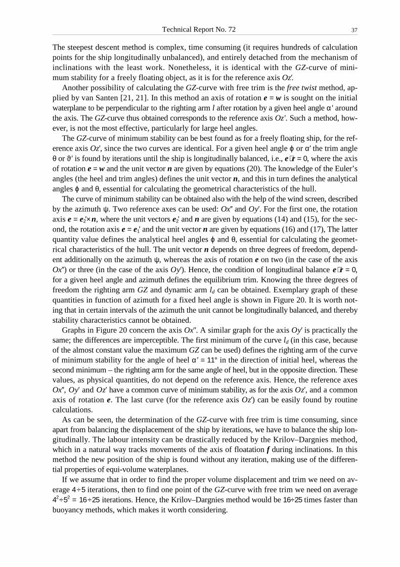
Technical Report No. 72
37
The steepest descent method is complex, time consuming (it requires hundreds of calculation points for the ship longitudinally unbalanced), and entirely detached from the mechanism of inclinations with the least work. Nonetheless, it is identical with the GZ-curve of mini-mum stability for a freely floating object, as it is for the reference axis Oz'.
Another possibility of calculating the GZ-curve with free trim is the free twist method, ap-plied by van Santen [21, 21]. In this method an axis of rotation e = w is sought on the initial waterplane to be perpendicular to the righting arm l after rotation by a given heel angle α' around the axis. The GZ-curve thus obtained corresponds to the reference axis Oz'. Such a method, how-ever, is not the most effective, particularly for large heel angles.
The GZ-curve of minimum stability can be best found as for a freely floating ship, for the ref-erence axis Oz', since the two curves are identical. For a given heel angle ϕ or α' the trim angle θ or ϑ' is found by iterations until the ship is longitudinally balanced, i.e., e ⋅ r = 0, where the axis of rotation e = w and the unit vector n are given by equations (20). The knowledge of the Euler’s angles (the heel and trim angles) defines the unit vector n, and this in turn defines the analytical angles ϕ and θ, essential for calculating the geometrical characteristics of the hull.
The curve of minimum stability can be obtained also with the help of the wind screen, described by the azimuth ψ. Two reference axes can be used: Ox'' and Oy'. For the first one, the rotation axis e = e2'× n, where the unit vectors e2' and n are given by equations (14) and (15), for the sec-ond, the rotation axis e = e1' and the unit vector n are given by equations (16) and (17), The latter quantity value defines the analytical heel angles ϕ and θ, essential for calculating the geomet-rical characteristics of the hull. The unit vector n depends on three degrees of freedom, depend-ent additionally on the azimuth ψ, whereas the axis of rotation e on two (in the case of the axis Ox'') or three (in the case of the axis Oy'). Hence, the condition of longitudinal balance e ⋅ r = 0, for a given heel angle and azimuth defines the equilibrium trim. Knowing the three degrees of freedom the righting arm GZ and dynamic arm ld can be obtained. Exemplary graph of these quantities in function of azimuth for a fixed heel angle is shown in Figure 20. It is worth not-ing that in certain intervals of the azimuth the unit cannot be longitudinally balanced, and thereby stability characteristics cannot be obtained.
Graphs in Figure 20 concern the axis Ox''. A similar graph for the axis Oy' is practically the same; the differences are imperceptible. The first minimum of the curve ld (in this case, because of the almost constant value the maximum GZ can be used) defines the righting arm of the curve of minimum stability for the angle of heel α' = 11° in the direction of initial heel, whereas the second minimum – the righting arm for the same angle of heel, but in the opposite direction. These values, as physical quantities, do not depend on the reference axis. Hence, the reference axes Ox'', Oy' and Oz' have a common curve of minimum stability, as for the axis Oz', and a common axis of rotation e. The last curve (for the reference axis Oz') can be easily found by routine calculations.
As can be seen, the determination of the GZ-curve with free trim is time consuming, since apart from balancing the displacement of the ship by iterations, we have to balance the ship lon-gitudinally. The labour intensity can be drastically reduced by the Krilov–Dargnies method, which in a natural way tracks movements of the axis of floatation f during inclinations. In this method the new position of the ship is found without any iteration, making use of the differen-tial properties of equi-volume waterplanes.
If we assume that in order to find the proper volume displacement and trim we need on av-erage 4 ÷5 iterations, then to find one point of the GZ-curve with free trim we need on average 42÷52 = 16 ÷25 iterations. Hence, the Krilov–Dargnies method would be 16÷25 times faster than buoyancy methods, which makes it worth considering.
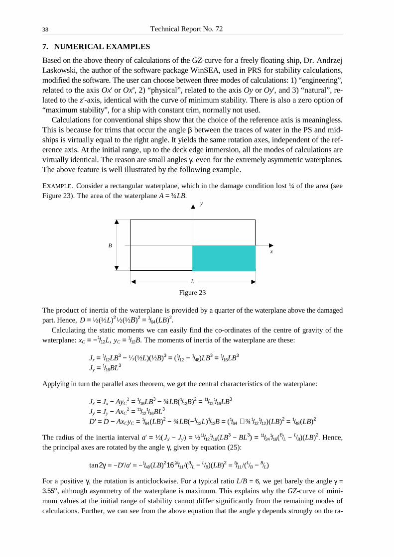
Technical Report No. 72
38
7. NUMERICAL EXAMPLES
Based on the above theory of calculations of the GZ-curve for a freely floating ship, Dr. Andrzej Laskowski, the author of the software package WinSEA, used in PRS for stability calculations, modified the software. The user can choose between three modes of calculations: 1) “engineering”, related to the axis Ox' or Ox'', 2) “physical”, related to the axis Oy or Oy', and 3) “natural”, re-lated to the z'-axis, identical with the curve of minimum stability. There is also a zero option of “maximum stability”, for a ship with constant trim, normally not used.
Calculations for conventional ships show that the choice of the reference axis is meaningless. This is because for trims that occur the angle β between the traces of water in the PS and mid-ships is virtually equal to the right angle. It yields the same rotation axes, independent of the ref-erence axis. At the initial range, up to the deck edge immersion, all the modes of calculations are virtually identical. The reason are small angles γ, even for the extremely asymmetric waterplanes. The above feature is well illustrated by the following example.
EXAMPLE. Consider a rectangular waterplane, which in the damage condition lost ¼ of the area (see Figure 23). The area of the waterplane A = ¾LB.
y
L
Bx
Figure 23
The product of inertia of the waterplane is provided by a quarter of the waterplane above the damaged part. Hence, D = ½(½L)2 ½(½B)2 = 1/64(LB)2.
Calculating the static moments we can easily find the co-ordinates of the centre of gravity of the waterplane: xC = −1/12L, yC = 1/12B. The moments of inertia of the waterplane are these:
Jx = 1/12LB3 − ⅓(½L)(½B)3 = (1/12 − 1/48)LB3 = 1/16LB3 Jy = 1/16BL3
Applying in turn the parallel axes theorem, we get the central characteristics of the waterplane:
Jx' = Jx − AyC2 = 1/16LB3 − ¾LB(1/12B)2 = 11/12
1/16LB3 Jy' = Jy − AxC
2 = 11/121/16BL3
D' = D − AxCyC = 1/64(LB)2 − ¾LB(−1/12L)1/12B = (1/64 + ¾1/121/12)(LB)2 = 1/48(LB)2
The radius of the inertia interval a' = ½(Jx' − Jy') = ½11/121/16(LB3 − BL3) = 11/24
1/16(B/L − L/B)(LB)2. Hence,
the principal axes are rotated by the angle γ, given by equation (25):
tan2γ = −D'/a' = −1/48(LB)216 24/11/(B/L − L/B)(LB)2 = 8/11 /(
L/B − B/L)
For a positive γ, the rotation is anticlockwise. For a typical ratio L/B = 6, we get barely the angle γ = 3.55°, although asymmetry of the waterplane is maximum. This explains why the GZ-curve of mini-mum values at the initial range of stability cannot differ significantly from the remaining modes of calculations. Further, we can see from the above equation that the angle γ depends strongly on the ra-
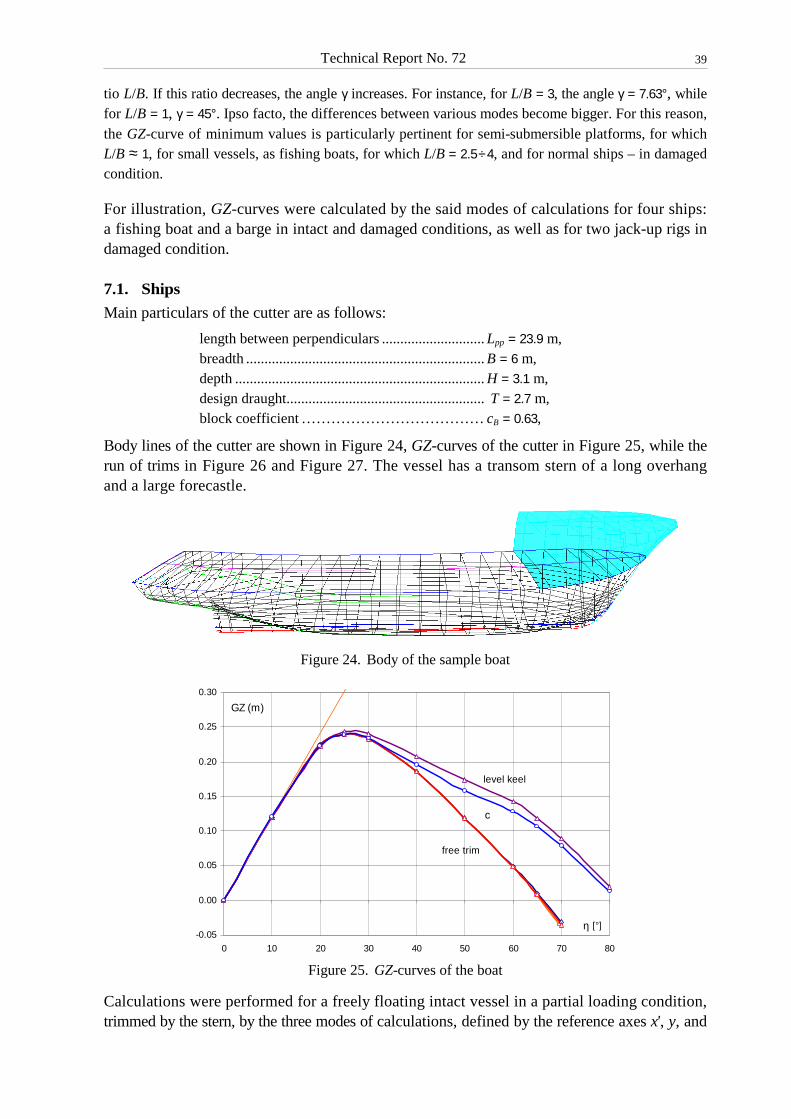
Technical Report No. 72
39
tio L/B. If this ratio decreases, the angle γ increases. For instance, for L/B = 3, the angle γ = 7.63°, while for L/B = 1, γ = 45°. Ipso facto, the differences between various modes become bigger. For this reason, the GZ-curve of minimum values is particularly pertinent for semi-submersible platforms, for which L/B ≈ 1, for small vessels, as fishing boats, for which L/B = 2.5÷4, and for normal ships – in damaged condition.
For illustration, GZ-curves were calculated by the said modes of calculations for four ships: a fishing boat and a barge in intact and damaged conditions, as well as for two jack-up rigs in damaged condition.
7.1. Ships
Main particulars of the cutter are as follows:
length between perpendiculars ............................Lpp = 23.9 m, breadth .................................................................B = 6 m, depth ....................................................................H = 3.1 m, design draught...................................................... T = 2.7 m, block coefficient ... . . . . . . . . . . . . . . . . . . . . . . . . . . . . . . .. . .cB = 0.63,
Body lines of the cutter are shown in Figure 24, GZ-curves of the cutter in Figure 25, while the run of trims in Figure 26 and Figure 27. The vessel has a transom stern of a long overhang and a large forecastle.
Figure 24. Body of the sample boat
-0.05
0.00
0.05
0.10
0.15
0.20
0.25
0.30
0 10 20 30 40 50 60 70 80
GZ (m)
c
free trim
level keel
η [°]
Figure 25. GZ-curves of the boat
Calculations were performed for a freely floating intact vessel in a partial loading condition, trimmed by the stern, by the three modes of calculations, defined by the reference axes x', y, and
Technical Report No. 72
40
z' in function of the appropriate angle of rotation η. In addition, calculations were performed for the ship with fixed trim, as at the position of equilibrium (curve c), and at level keel.
As can be seen from Figure 25, at the initial range of stability (up to the angle ηmax, at which the GZ-curve reaches maximum) all the calculation modes yield the same results. The differences start above ηmax. As expected, the highest values of the GZ-curves for large heel angles (in the sloping part) are obtained for the ship at level keel, greatly overestimating the range of stability. Somewhat smaller values are obtained for the ship with fixed trim, as at the initial position (curve c). Both curves converge at the heel angle 90°.
As should be expected, the least GZ-curves are obtained for the ship with free trim, wherein these curves are practically unaffected by the way the ship is balanced. Hence, the choice of the reference axis has no meaning. These curves practically collapse into one curve, as the correspond-ing run of trims, measured in the PS, is practically identical (Figure 26), irrespective of the ref-erence axis, which entails virtually the same rotation axes e (the angles between them γ1 ≈ γ3 ≈ 0) and heel angles (rotations of the planes of rotation). Free trim rapidly increases for heel angles larger than 30°. Therefore, curve c up to this angle coincides with the GZ-curves with free trim, well visible in Figure 25. As should be expected, curve c and curve for level keel converge. The curves in Figure 25 resemble those in Figure 1.
-6
-5
-4
-3
-2
-1
0
0 10 20 30 40 50 60 70
y
t (m)c
z
x
η [°]
0
1
2
3
4
0 10 20 30 40 50 60 70
α' [°]
ϑ' [°]
Figure 26. Run of trims in PS during heeling the
boat, depending on the reference axis Figure 27. Run of twist angle around
axis Oz' during heeling the boat
Figure 27 shows the run of the angle of twist (trim) for the reference axis Oz' in terms of the angle of heel for the boat inclined to starboard. As can be seen, for intact symmetric boats the angle of twist does not assume large values (in this case does not exceed 4°), and for inclinations to portside the twist would be the same but of the opposite sign.
Figure 28 shows the run of stability characteristics for the cutter in function of the angle of twist Ψ for a given heel angle α' = 55°. The curves GZ and ld are symmetric and the curve le = e ⋅ r is antisymmetric with respect to the angle Ψ = 90° and 270°. After rotation by an angle Ψ = 90° or 270° PS coincides with the plane of rotation, resulting in a longitudinal balance of the ship. The righting arm and the dynamic arm reach then their maximum. This is a feature of intact ships, with no initial heel, having a PS. In the range Ψ ∈ (0°, 180°) the bow is immersed in water and the stern is above, while in the range Ψ ∈ (180°, 360°) it is vice versa. At a point Ψ = 0, the ship is inclined towards starboard, and at a point Ψ = 180°, towards portside.
It is worth paying attention to the curve le = e⋅r, i.e. the longitudinal component of the righting arm. From equation (42) it follows that its derivative ∂le/∂Ψ = −HLϑ. This curve has an oscilla-tory character with respect to the twist angle Ψ, which entails the oscillatory character of the longitudinal metacentric height HLϑ. In the extreme points of le the longitudinal metacentric

Technical Report No. 72
41
height vanishes, i.e. HLϑ = 0. We can see from Figure 28 that zeros of curve le define not only the extremes of the curve of dynamic arms and righting arms, but they are also points of in-flexion, i.e. the extremes of the longitudinal metacentric height HLϑ. In the increasing part HL < 0 is negative and decreasing HLϑ > 0 positive. In the first and third equilibrium position, with minimum potential energy, there is a stable equilibrium (HLϑ > 0), whereas in the second and fourth – unstable (HLϑ < 0).
-6
-4
-2
0
2
4
6
0 45 90 135 180 225 270 315 360
α' = 55°°
Ψ [°]
GZ
le = e⋅r
[m]
ld
Figure 28. Run of transverse and longitudinal components of the righting arm
and dynamic arm ld for the boat versus angle of twist Ψ for α' = 55°
The cutter is a small boat. We will now see stability characteristics for a large vessel, i.e. the barge investigated by van Santen [20]. Its main dimensions L×B×H×T = 140×36 ×8,5×5 m, KG = 17 m. The barge has a forecastle with dimensions: l×h = 25 × 8 m (Figure 29). Both units have almost the same ratio L/B, close to 4. The GZ-curves of the barge are shown in Figure 30, the run of trims in Figure 31, and the run of twist ϑ in Figure 32.
Figure 29. Barge
As for the cutter, GZ-curves (Figure 30) and trims t (Figure 31) do not depend on the choice of the reference axis. However, contrary to the cutter, after immersing the deck edge in water (η = 11°) the differences between the GZ-curve at level keel and with free trim are modest. This is because of the proportionally smaller forecastle. As for the cutter, trims in terms of angles are small (Figure 32). For a heel angle α = 35°, the twist angle equals merely ϑ = 2,3°. In general, for symmetric units GZ-curves for inclinations to the other side are anti-symmetric.

Technical Report No. 72
42
-1
0
1
2
0 5 10 15 20 25 30 35 40
GZ (m)
free trim
level keel
η [°]
Figure 30. GZ-curves of intact barge
-5
-4
-3
-2
-1
0
1
0 10 20 30 40
t (m)
η [°]
Figure 31. Run of trims in PS during heeling the barge, depending on the reference axis
-0.5
0
0.5
1
1.5
2
2.5
0 10 20 30 40
α [°]
ϑ [°]
Figure 32. Run of twist ϑ around axis z during heeling the barge
Figure 33 shows the run of stability characteristics for the barge as functions of the twist angle Ψ for a chosen heel angle α = 20°. The nature of these curves is similar to those for the cutter.

Technical Report No. 72
43
-40
-30
-20
-10
0
10
20
30
40
50
0 45 90 135 180 225 270 315 360
α = 20°°
Ψ [°]
GZ
le = e⋅r
[m]
2ld
Figure 33. Run of transverse and longitudinal components of the righting arm
and dynamic arm ld for barge versus angle of twist Ψ for α = 20°
For comparative purposes stability of the barge was analysed also in damage condition with a flooded compartment of dimensions l×b×h = 14 ×7,2×4,5 m, adjacent to the aft, bottom and starboard (Figure 34). As in the previous cases, the GZ-curves (Figure 35) and trims do not depend on the reference axis. A larger difference occurs now between the GZ-curve for a freely floating ship and the curve at level keel than in the intact case.
For damaged units, asymmetrically flooded, GZ-curves for inclinations on both sides are different. When inclined against the initial heel they are larger, see Figure 36.
The run of the angle of twist ϑ' and stability characteristics for the damaged barge is very similar to those shown in Figure 32 and Figure 33, therefore these graphs will not be shown. In both cases, for any heel angle the curve le has four zeros, wherein the first and third zeros are symmetric relative to the angle 90°. As we will see, the existence of the GZ-curve for a freely floating ship inclined to either side is contingent on the above. Because of the initial heel the GZ-curve for the reference axis Oz' is indefinite in the neighborhood of zero on the side oppo-site to initial heel. According to equation (43) this interval starts exactly at zero and ends at the angle α' = −0,10°, which cannot be perceived.
Figure 34. Damaged barge

Technical Report No. 72
44
-2.0
-1.0
0.0
1.0
2.0
-5 0 5 10 15 20 25 30 35
GZ (m)
free trim
level trim
η [°]
Figure 35. GZ-curves for damaged barge for inclinations to starboard
-2
-1
0
1
2
-40 -30 -20 -10 0 10 20 30 40
l (m)
level keel
η [°]
level keel
free trimfree trim
Figure 36. GZ-curves for damaged barge for inclinations to both sides
7.2. Jack up rigs
There were two rigs investigated I and II. Main particulars of the first one are as follows: length .................................................................................................L = 73.659 m, breadth ...............................................................................................B = 54.222 m, depth ..................................................................................................H = 6.755 m, draught...............................................................................................T = 5 m, waterplane coefficient of fineness .... . . . . . . . . . . . . .. . . . . . . . . . . . . . . . . . . . .cW = 0.668. ratio of waterplane principal moments of inertia in the upright........Jy/Jx = 1.73.
The platform is shown in Figure 37, GZ-curves are shown in Figure 38, while the run of trims is given in Figure 39 to Figure 41. Calculations were performed for a damaged platform, trimmed by aft, and inclined to starboard with a heel of 2°, for the same modes, as for the cutter, for incli-nations to starboard.
As can be seen from Figure 38, similarly as in the previous case, all the calculation modes at the initial range of stability yield the same values of the righting arms. Some visible differ-ences refer solely to the platform at level keel. They result from the fact that – due to asym-

Technical Report No. 72
45
metric flooding – the principal axis of inertia of the waterplane is deviated from the PS, while this mode assumes the axis of rotation parallel to the PS.
Figure 37. Jack-up platform I
-1
0
1
2
0 4 8 12 16 20
GZ (m)
fixed trim trim
free trim
η [°]
x'y
z'
rotation angle
c
Figure 38. GZ-curves for platform I inclined to starboard
(in the direction of initial heel)
The largest righting arms yield the platform at level keel, largely overestimating the range of stability. Somewhat smaller values are obtained for the ship with fixed trim, the same as at the initial position. Both curves converge, when the heel angle tends to 90°.
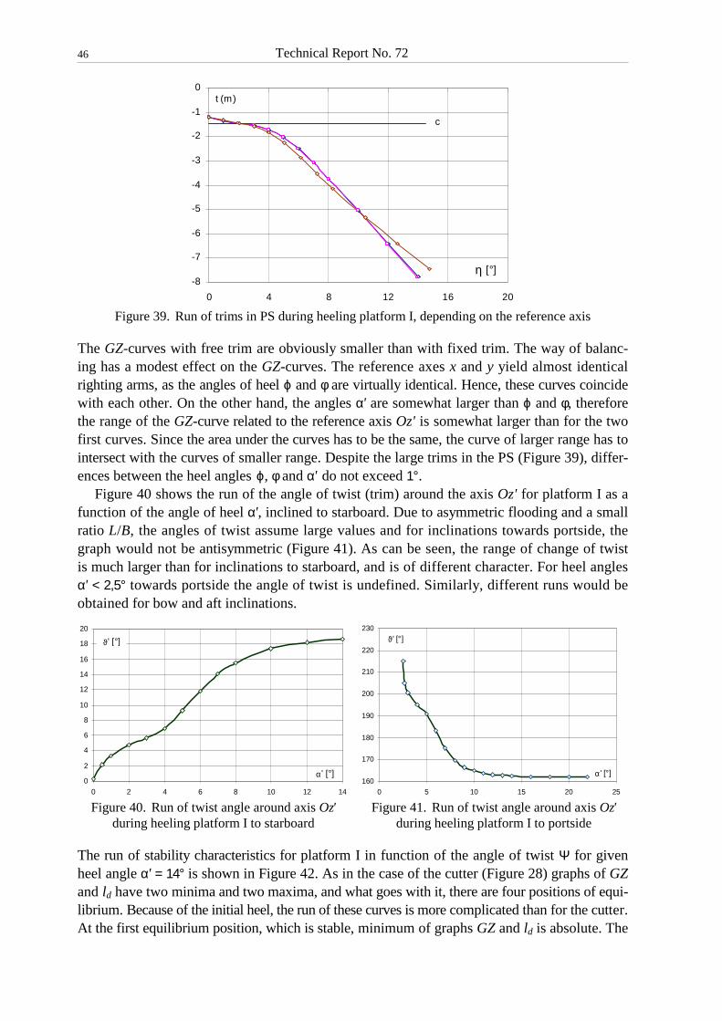
Technical Report No. 72
46
-8
-7
-6
-5
-4
-3
-2
-1
0
0 4 8 12 16 20
t (m)
c
η [°]
Figure 39. Run of trims in PS during heeling platform I, depending on the reference axis
The GZ-curves with free trim are obviously smaller than with fixed trim. The way of balanc-ing has a modest effect on the GZ-curves. The reference axes x and y yield almost identical righting arms, as the angles of heel ϕ and φ are virtually identical. Hence, these curves coincide with each other. On the other hand, the angles α' are somewhat larger than ϕ and φ, therefore the range of the GZ-curve related to the reference axis Oz' is somewhat larger than for the two first curves. Since the area under the curves has to be the same, the curve of larger range has to intersect with the curves of smaller range. Despite the large trims in the PS (Figure 39), differ-ences between the heel angles ϕ, φ and α' do not exceed 1°.
Figure 40 shows the run of the angle of twist (trim) around the axis Oz' for platform I as a function of the angle of heel α', inclined to starboard. Due to asymmetric flooding and a small ratio L/B, the angles of twist assume large values and for inclinations towards portside, the graph would not be antisymmetric (Figure 41). As can be seen, the range of change of twist is much larger than for inclinations to starboard, and is of different character. For heel angles α' < 2,5° towards portside the angle of twist is undefined. Similarly, different runs would be obtained for bow and aft inclinations.
0
2
4
6
8
10
12
14
16
18
20
0 2 4 6 8 10 12 14
ϑ' [°]
α' [°]
160
170
180
190
200
210
220
230
0 5 10 15 20 25
α' [°]
ϑ' [°]
Figure 40. Run of twist angle around axis Oz'
during heeling platform I to starboard Figure 41. Run of twist angle around axis Oz'
during heeling platform I to portside
The run of stability characteristics for platform I in function of the angle of twist Ψ for given heel angle α' = 14° is shown in Figure 42. As in the case of the cutter (Figure 28) graphs of GZ and ld have two minima and two maxima, and what goes with it, there are four positions of equi-librium. Because of the initial heel, the run of these curves is more complicated than for the cutter. At the first equilibrium position, which is stable, minimum of graphs GZ and ld is absolute. The

Technical Report No. 72
47
third equilibrium position corresponds to inclinations to the other side. Four zeros of the curve le means that the righting arms GZ exist for inclinations in both directions. In the case of rigs it does not have to be so. For certain heel angles the curve le can have only two zeros, as in Figure 43, with one minimum for the dynamic arm ld.
-3
-2
-1
0
1
2
3
4
5
0 45 90 135 180 225 270 315 360
GZ
le = e⋅r
α' = 14°°
Ψ [°]
[m]
2ld
Figure 42. Run of transverse and longitudinal components of the righting arm
and dynamic arm ld for platform I versus angle of twist Ψ for α' = 14°
-1.5
-1
-0.5
0
0.5
1
1.5
2
2.5
0 45 90 135 180 225 270 315 360
GZ
le = e⋅r
α' = 2°°
Ψ [°]
[m]
15ld
B
Figure 43. Run of stability characteristics for platform I in function of twist Ψ for α' = 2°
In the case of rig I such a situation occurs for heel angles α' < 2,5° (at the angle α' = 2,5° point B in curve le becomes tangent to the abscissa axis). It means that for inclinations to portside the rig cannot be longitudinally balanced, and thereby the free trim GZ-curve cannot be obtained, nor the angle of twist. Note that at the range of Ψ ≈ 165°÷215° (Figure 43), i.e. at the flat segment of le up to point B a neutral equilibrium occurs, with the longitudinal metacentric height HLϑ ≈ 0, whereas above this point – unstable. In such a case, the rig will turn spontaneously by 180° around the axis Oz' to assume a stable position, corresponding to the first zero of the curve le, inclined to starboard, where the only minimum of potential energy occurs – minimum of the dynamic arm ld.

Technical Report No. 72
48
For inclinations to starboard the GZ-curve exists in the whole range (Figure 38). For incli-nations to portside, the GZ-curve exists for α' < −2,5°, i.e. when the third zero of the curve le exists, associated with positive metacentric height HLϑ > 0 (approximated equation (43) yields the angle α' = −1,9°). Intuitively, everybody would expect that for inclinations against the initial heel the stability is better. It is so, but for heel angles α' < −2,5° (Figure 44), which is better seen in Figure 46 – the range of stability and the maximum lever are markedly larger than for inclinations to starboard.
-3
-2
-1
0
1
-24 -20 -16 -12 -8 -4 0 4
GZ (m)
η [°]
z'
Figure 44. GZ-curve for platform I inclined to portside for axis Oz'
However, for heel angles α' ∈ ⟨−2,5°, 0⟩, the GZ-curve does not exist, due to the lack of longi-tudinal stability, unless the rig will rotate by 180° around the Oz' axis, assuming values as for inclinations to starboard (Figure 5). For other reference axes, such a problem does not exist – GZ-curves exist for any angle of heel to portside (Figure 45, Figure 46), wherein they complete the free trim GZ-curve for the axis Oz' at the range, where it is indefinite.
-3
-2
-1
0
1
-24 -20 -16 -12 -8 -4 0 4
GZ (m)
η [°]
x' y
z'
rotation angle
Figure 45. GZ-curves for platform I inclined to portside
From equation (42) it follows that at an upright position α' = 0 the metacentric height HLϑ is discontinuous; on one side of zero it is positive and the GZ-curve exists, and on the other side it is negative and the GZ-curve does not exist in a certain range, which can be seen in Figure 44. This is a feature of freely floating ships with an initial heel, which is contradictory to intuition.

Technical Report No. 72
49
-3
-2
-1
0
1
2
-24 -20 -16 -12 -8 -4 0 4 8 12 16 20
GZ (m)
η [°]
level trim
free trim
c
x'y
z'
rotation angle
z'
level trim
free trim
x' y
Figure 46. GZ-curves for rig I for inclinations to both sides
Main particulars of platform II are as follows:
length ............................................................................ L = 58,1 m, maximum breadth .........................................................B0 = 72,2 m, minimum breadth..........................................................B1 = 14 m, depth ............................................................................. H = 7 m, draught .......................................................................... T = 4.65 m, waterplane coefficient of fineness .... . . . . . . . . . . . . .. . . . . . cW = 0.597, height of centre of gravity above BP............................KG = 24.37 m, ratio of waterplane principal moments of inertia in an upright position....................................................Jy/Jx = 1.06.
Figure 47. Platform II
This is a fictitious jack-up platform of simple geometric shape (Figure 47), conceived by ABS for testing calculations, widely investigated in literature [20, 23, 24]. GZ-curves are shown in Figure 48, while the run of trims in Figure 49 and Figure 50. Calculations were performed for a dam-aged platform, trimmed by aft (t = −2.058 m), inclined to starboard with a heel 1.73°.

Technical Report No. 72
50
-1
0
1
2
0 2 4 6 8 10 12 14
GZ (m) level trim
free trim
rotation angle η [°]
x'y z'
fixed trim
c
Figure 48. GZ-curves of rig II inclined to starboard
As can be seen from Figure 48, all the calculation modes yield practically the same values of GZ-curves at the initial range of stability. Above this range, the largest values correspond to the platform at level keel. As in the case of platform I, the way of balancing has only a modest effect on GZ-curves. The GZ-curves for the reference axes x and y, as before, are almost identical, as the heel angles ϕ and φ, despite the large trims in the PS (Figure 49), are virtually the same, which means the axes of rotation are almost parallel. Hence, these curves coincide with each other. On the other hand, the heel angles α' are somewhat larger than the angles ϕ and φ, which results – as before – in a somewhat larger range of stability. Since the area under the curves has to be the same, the curve of larger range intersects with the curves of smaller range, and it has a smaller GZmax value. If the axes of rotation for the reference axes Ox'', Oy' and Oz' are the same, then the GZ-curves correspond to minimum stability. This observation confirms Figure 48, where the three curves collapse into one curve.
-9
-8
-7
-6
-5
-4
-3
-2
-1
0 2 4 6 8 10 12 14
t (m)
c
x'
y
z'
η [°]
Figure 49. Run of trims in PS during heeling rig II, depending on the reference axis
Figure 50 shows the run of the angle of twist (trim) around the axis Oz' in function of the angle of heel. Because of an asymmetric flooding and a small ratio L/B, these angles assume yet larger values than for platform I. But the waterplane is symmetric, therefore twist (rotation) of the platform starts above the angle at which the deck enters the water. As before, the graph has a dif-ferent character for inclinations to portside (Figure 51). The range of change of the twist angle for inclinations to portside equals 16°, while to starboard equals 26°. For heel angles α' < 7,4°
Technical Report No. 72
51
to portside the twist angle is indefinite. It means that in the range α' ∈ ⟨−7,4°, 0⟩ the GZ-curve is indefinite (the approximated equation (43) yields the angle α' = −3.1°).
-5
0
5
10
15
20
25
30
0 2 4 6 8 10 12 14
ϑ' [°]
α' [°]
125
130
135
140
145
-18 -16 -14 -12 -10 -8 -6 -4
α' [°]
ϑ' [°]
Figure 50. Run of twist around axis Oz'
during heeling rig II to starboard Figure 51. Run of twist around axis Oz'
during heeling rig II to portside
The run of stability characteristics for rig II in function of the angle of twist Ψ for a heel angle α' = 11° is shown in Figure 19. Similarly, as in the case of rig I (Figure 42) there are also four equilibrium positions, corresponding to extreme values of the righting arm l = GZ and dynamic arm ld. However, the GZ-curve has two additional extreme points, corresponding to points of inflexion on the curve of dynamic arms ld. The reason for this strange behaviour is a small ratio of the principal moments of inertia of the waterplane in an upright position, close to 1. For rig II this ratio equals 1.06, whereas for rig I equals 1.73. Nonetheless, as in the previous cases, at the first equilibrium position minima of the curves GZ and ld are the lowest, while the third equilibrium position corresponds to the heel to portside, wherein both are symmetric relative to the angle 90°.
From Figure 19 it follows that for platform II a surface of dynamic arms ld = ld(α', Ψ), termed also as the energy to heel surface, should have two valleys (paths), corresponding to minimum ld. Meanwhile, Figure 22 shows three paths (three minima). Admittedly, both figures correspond to different reference axes, but the choice of the reference axis has no significant effect on the dynamic arms.
Figure 52 shows the run of stability characteristics for a different heel angle α' = 6°. The run differs from that for the angle α' = 11° (Figure 19). The curve le has now only two zeros, instead of four. The zeros precisely coincide with the extremes of the curve of dynamic arms ld but they are clearly shifted off from the extremes of the GZ-curve. Apex B of the curve le becomes tan-gent to the abscissa axis at the angle α' ≈ 7,4°. Hence, for heel angle α' > 7,4° there are again four zeros of the curve le (Figure 19), which is a condition for the existence of the GZ-curve for inclinations to portside. At the range α' < 7,4°, i.e. α' ∈ ⟨−7,4°, 0⟩ this curve does not exist (Figure 54), unless the rig turns by 180° around the axis Oz', assuming values as for heels to starboard. Due to a yet smaller ratio of the principal moments of inertia of the waterplane at an upright position and a larger asymmetry of flooding (a large negative righting arm at an upright position), the range in which the GZ-curve is indefinite due to the lack of longitudinal balance, is bigger than in the previous case, which results also from the approximated equation (43). For the reference axes Ox' and Oy the GZ-curve do not exist for heel angles below −13° (Figure 53, Figure 54). However, they are not the curves of minimum stability.

Technical Report No. 72
52
-2
-1
0
1
2
3
4
0 45 90 135 180 225 270 315 360
α' = 6°° l = GZ
le = e⋅r
[m]
8ld
B
Ψ [°]
Figure 52. Run of GZ, le and ld for platform II versus angle of twist Ψ for α' = 6°
-3
-2
-1
0
1
-18 -16 -14 -12 -10 -8 -6 -4 -2 0 2
GZ (m)
x' yz'
rotation angle η [°]
Figure 53. GZ-curves of platform II for inclinations to portside
-4
-3
-2
-1
0
1
2
3
-20 -16 -12 -8 -4 0 4 8 12 16
GZ (m)
η [°]
level trim
x'y z'
rotation angle
cz' free trim
free trim
level trim
x' y
c
Figure 54. GZ-curves of platform II for inclinations to both sides
The angle of twist Ψ and GZ-curve and for inclinations to portside are shown in Figure 51 and Figure 53. As discussed earlier, these characteristics exist for the angle α' < −7,4°. They were obtained as readings for the third zero of the curve le, as in Figure 19. An identical curve can be obtained from direct calculations for inclinations to portside.

Technical Report No. 72
53
Figure 55 shows the run of stability characteristics for a heel angle α' = 6° in function of the azimuth for the reference axis Ox''. We can see that these characteristic differ for the reference axis Oz' (Figure 52). Nonetheless, they both indicate the same features. Also here, due to the fact that the angle of heel α' = 6° is below the critical value 7.4°, a graph of the dynamic arm ld in function of the azimuth has only one minimum. It defines a righting arm of the curve of minimum stability for the angle α' = 6° in the direction of the initial heel, identical with that in Figure 52. The lack of the second minimum means that for a heel on the other side the righting arm does not exist. As we know from the proceeding considerations, in the range of α' ∈ ⟨−7,4°, 0°⟩ the GZ-curve does not exist, as in this range of heel angles the ship cannot be longitudinally balanced. From Figure 55 it follows additionally that for the heel angle α' = 6° the rig cannot be longitudinally balanced, if the azimuth is from the range of ψ ∈ ⟨86°, 106°⟩.
0
1
2
3
4
0 45 90 135 180 225 270 315 360
GZ
GZ ld
ld
[m]
ψ [°]
α' = 6°
le
Figure 55. Run of righting arm GZ and dynamic arm ld for platform II
versus azimuth Ψ for heel angle less than critical
In the case of asymmetrically flooded units the extremes of GZ-curves are somewhat shifted relative to the equilibrium position. It can be shown that there is no shift, if the axis of rotation e is parallel to the principal axis of inertia of the waterplane. A proof is simple – we have to differentiate with respect to trim the righting arm l ≡ GZ, given by equation (22). Considering that the unit vector of the axis of rotation e need not be differentiated, we get the equation:
l' = e ⋅ (r' × n) + e ⋅ (r × n' )
where ' stands for the differentiation with respect to trim. It can be easily shown differentiating with respect to ϑ the unit vector n, given by equation (54), that the vector n' = sinαe is parallel to the axis of rotation e, therefore the second term vanishes on the virtue of properties of the scalar triple product. Further, the vector r' has two components: longitudinal and transverse. A con-tribution to the triple product gives only the transverse component r'T = −n × eD''/V, where the differentiation is with respect to trim τ, and D'' is the product of inertia of the waterplane in the ξ''η'' system (Figure 11), parallel to the axis of rotation e. Hence,
∂/∂τ GZ = −D''/V (60)
It follows from equation (60) that at the equilibrium position an extreme of the GZ-curve oc-curs, if D'' = 0, i.e. when the principal axis of inertia of the waterplane is parallel to the axis of

Technical Report No. 72
54
rotation e. In the case of conventional ships, even in the damaged condition, the deviation of the principal axis of inertia from the axis of rotation e is small; therefore a shift of the extreme of GZ relative to the equilibrium position is imperceptible. In the case of damaged rigs with four zeros of the curve le, the shift is not large, but noticeable (Figure 19, Figure 42), whereas in the case of two zeros, a clear shift is visible (Figure 43, Figure 52).
It is interesting to see the run of the same stability characteristics in function of the twist angle for the same fixed heel angle α', but for an intact rig II. Such a graph is shown in Figure 56.
-2
-1
0
1
2
3
4
5
0 45 90 135 180 225 270 315 360
α' = 11°°
GZ
le = e⋅r
[m]
4ld
Ψ [°]
Figure 56. Run of stability characteristic for intact rig II
in function of twist Ψ, for α' = 11°
As in the case of intact ships with no initial heel angle the curves GZ and ld are symmetric, while the curve le = e ⋅ r is asymmetric with respect to the angle Ψ = 90° and 270°. However, unlike for the cutter (Figure 28), there are two additional points of longitudinal equilibrium, where the GZ-curve and dynamic curve ld have extremes. Hence, in this case, the energy sur-face ld = ld(α', Ψ) would have three valleys, corresponding to minimum ld. The two first min-ima, corresponding to inclinations to portside and starboard, are equal to each other but are smaller from the third minimum.
8. CONCLUSIONS
The paper presents the theoretical basis for determination of the GZ-curve for a freely floating ship, longitudinally balanced at each heel angle. Three modes of calculations of the GZ-curves were discussed: 1) “engineering”, related to the axis x' or x'', 2) “physical”, related to the axis y or y', and 3) “natural”, related to the z'-axis, identical with minimum stability. Based on the results of theoretical and numerical analysis, the following conclusions can be drawn:
a) a freely floating ship has minimum stability in the sense of the area under the GZ-curve. The said area is independent of the reference axes and is the smallest possible
b) balancing of the ship does not change in space the direction of the righting moment, but de-creases its value in proportion to change of trim after balancing
c) at the initial range of stability all the modes of calculations (including the mode of fixed trim) yield practically the same results
d) for conventional ships the GZ-curves are independent of the reference axis (the way of balancing), while for platforms the effect is modest
Technical Report No. 72
55
e) if the ship has an initial heel, the GZ-curve is indefinite in some one-sided neighborhood of zero, opposite to the initial heel, whose length increases with the initial heel. For ships, it is of the order of angular minutes, and for platforms – of the order of degrees. The azimuth (twist) of the unit in this range of heel is unstable, i.e., the unit can rotate automatically around the axis Oz' to assume a stable heel towards the initial heel
f) for freely floating units only one GZ-curve is meaningful, of minimum stability, as for the reference axis Oz'. For other azimuths, they can have gaps in which they are indefinite
g) the notion of cross-curves of stability is also valid for a freely floating ship with minimum stability, when the ship's centre of gravity varies along the axis Oz', normal to the initial waterplane
h) it is advisable to perform calculations of the GZ-curve by means of equi-volume waterplane method (Krilov–Dargnies), inclined around the instantaneous axis of floatation f. It cuts radically the time of calculations (16 ÷ 25 times) in comparison to buoyancy methods, as it needs no iterations
Thence, for ships there is no revolution – any method of calculating the GZ-curve with free trim yields virtually the same curve, identical with minimum stability. There is, however, a revolu-tionary conclusion for platforms – there is only one meaningful GZ-curve, related to transverse inclinations, as for the reference axis Oz'. In other words, for rigs there are no GZ-curves for various azimuths, required by regulations. In the case of the reference axis Oz' they are the same, irrespective of the azimuth, while for other reference axes they have, admittedly larger values but at the cost of instable intervals, in which the ship cannot be longitudinally balanced. Hence, what sort of curves has been calculated? Either for rigs with fixed trim, or improperly balanced. The latter is very probable; as such notions as the reference axis, axis of rotation, plane of rotation, and angle of rotation of the plane of rotation are not mentioned in literature. Interesting papers, for instance [20, 21, 23, 24] do not clearly state in which plane the rig was balanced.
ACKNOWLEDGEMENTS
The work evolved over a number of years. The introduction to the area of a freely floating ship comes from the unique book [22]; developed further in works [4–7], carried out mainly during the author’s visits to Glasgow University (1987) and the University of Newcastle upon Tyne (1992). Incentive for the systematic development of this research came from the author’s in-volvement in the IMO SLF Sub-Committee in the years 1979–1996. Mr. Joost van Santen is acknowledged for validating numerical calculations for the cutter.
REFERENCES
1. W i m a l s i r i W. K. Design of ro-ro cargo ships with particular reference to damage survivabil-ity, PhD thesis, Dept. of Marine Technology, University of Newcastle upon Tyne, 1991.
2. V a s s a l o s D., K o n s t a n t o p o u l o s G., K u o C., W e l a y a Y. A realistic ap-proach to semisubmersible stability, SNAME Transactions, Vol. 93, 1985, pp. 96–128.
3. S a n t e n v a n J. A. Stability calculations for jack-ups and semi-submersibles, Conference on Computer Aided. Design, Manufacturer and Operation in the Marine and Offshore Industries – CADMO ‘86, Washington D.C., Sept. 1986.
4. P a w ł o w s k i M. On the roll angle for a freely floating rig, Proceedings, 9th Intl. Symposium on Ship Hydromechanics HYDRONAV '91, Sarnówek, September 1991, Vol. I, pp. 23–26; also in:

Technical Report No. 72
56
Budownictwo Okrętowe i Gospodarka Morska, Vol. 36, November 1991, no 11(397), pp. 24–26, ISSN 0007-3008.
5. P a w ł o w s k i M. Some inadequacies in the stability rules for floating platforms, The Naval Ar-chitect, No. 2, 1992, pp. 889–894.
6. P a w ł o w s k i M. Advanced stability calculations for a freely floating rig, Proceedings, 5th Intl. Symposium on Practical Design of Ships and Mobile Units PRADS ′92, Newcastle upon Tyne, 1992, Vol. II, pp. 1146–1160; also in: Report, Dept. of Marine Technology, University of Newcastle upon Tyne, November 1991, 31 pp.
7. P a w ł o w s k i M. Stability of free floating ship, Part I, Polish Maritime Research, 2005,, Vol. 12, No. 2, pp. 3–9, Part II, Vol. 12, No. 3 (2005), pp. 3–8, ISSN 1233-2585.
8. B o u g u e r P. Traité du navire, de sa construction et de ses mouvemens (Treatise of the ship, its construction and its movements), Jombert, Paris, 1746.
9. A t w o o d G. The construction and analysis of geometrical propositions, determining the posi-tions assumed by homogenous bodies which float freely, and at rest on a fluid’s surface; also De-termining the stability of ships and of other floating bodies, Philosophical Transactions of the Royal Society of London, Vol. 86, pp. 46-278, 1796.
10. K a ź m i e r c z a k J. Pływalność i stateczność okrętu, Warszawa, Wydawnictwa Komunikacyjne, 1954.
11. S t a l i ń s k i J. Teoria okrętu, Gdynia, Wydawnictwo Morskie, 1961.
12. R e e d E. A treatise on the stability of ships, London, Charles Griffin & Co., 1885.
13. R a h o l a J. The judging of the stability of ships and the determination of the minimum amount of stability, PhD thesis, University of Helsinki, 1939
14. International Maritime Organisation: International code on intact stability, London, IMO 2008 (2009 Edition), ISBN 978-92-801-15062.
15. International Maritime Organisation: Subdivision and damage stability of cargo ships, SOLAS Con-vention, Consolidated Edition 1997, chapter II–1, part B–1, pp. 89–99, London, ISBN 92-801-1433-6
16. P a w ł o w s k i M. A closed form assessment of the capsizal probability – the si factor, Proceed-ings, WEGEMT Workshop on Stability of Ships, Technical University of Denmark (DTU), Lyngby, October 1995, 11 pp.
17. V a s s a l o s D., P a w ł o w s k i M., T u r a n O. Criteria for survival in damaged condition, Proceedings, Intl. Seminar on the Safety of ro-ro Passenger Vessels, RINA, London, June 1996, 15 pp.; also in: Dynamic stability assessment of damaged passenger ro-ro ships and proposal of rational sur-vival criteria, Marine Technology, Vol. 34, No. 4, October 1997, pp. 241–266.
18. P a w ł o w s k i M. A modified static equivalency method for roll-on/roll-off vessels, Journal of Ship Research, Vol. 51, No. 1, March 2007, pp. 39–46.
19. P a w ł o w s k i M. Survival criteria for passenger ro–ro vessels and survival time, Marine Tech-nology, Vol. 44, No. 1, January 2007, pp. 27–34.
20. S a n t e n v a n J. A. The use of energy build up to identify the most critical heeling axis direction for stability calculations for floating offshore structures, Proceedings, 10th Intl. Conf. on Stability of Ships and Ocean Vehicles STAB 2009, Sankt Petersburg, 22–26 June 2009, pp. 65–76.
21. S a n t e n v a n J. A. Problems met in stability calculations of offshore rigs and how to deal with them, Proceedings, 13th Intl. Ship Stability Workshop, Brest, 23–26 September 2013, 9 pp.
22. S i e m i o n o v - T i a n - S h a n s k y W. W. Статикa и динамика корабля, Leningrad, Sudpromgiz, 1960, also in: Statics and dynamics of ships, Moscow, Peace Publishers, 1963.
Technical Report No. 72
57
23. B r e u e r J. A., S j ö l u n d K. G. Orthogonal tipping in conventional offshore stability evalua-tions, Proceedings, 9th Intl. Conf. on Stability of Ships and Ocean Vehicles STAB 2006, Rio de Janeiro, 25–29 September 2006, pp. 817–828
24. B r e u e r J. A., S j ö l u n d K. G. Steepest descent method – resolving an old problem, Pro-ceedings, 10th Intl. Conf. on Stability of Ships and Ocean Vehicles STAB 2009, Sankt Petersburg, 22–26 June 2009, pp. 87–99 ■
Appendix – Transformation of moments of inertia
Elements of the inertia tensor in the system x'y', rotated with respect to the system xy by an angle α, are given by the following expressions:
Jx'x' = Jxxcos2α + Jyysin2α + Jxysin2α Jy' = Jycos2α + Jxsin2α + Dsin2α
Jy'y' = Jxxsin2α + Jyycos2α − Jxysin2α Jx' = Jysin2α + Jxcos2α − Dsin2α
Jx'y' = ½(Jyy − Jxx)sin2α + Jxycos2α D' = ½(Jx − Jy)sin2α + Dcos2α
These expressions have double notations: in the first row there is a tensor notation, while in the second – a geometric (engineering) notation.
Introducing the notation: a = ½(Jx − Jy) for a radius of the inertia interval (in naval applica-tions the radius a is normally negative), and s = ½(Jx + Jy) for a centre of the interval, which yields Jx = s + a, Jy = s − a, the above expressions take the form:
Jx' = s + acos2α − Dsin2α ≡ s + a' Jy' = s − acos2α + Dsin2α ≡ s − a' D' = asin2α + Dcos2α.
As can be seen, the trace of the tensor is conserved, i.e. Jx'x' + Jy'y' = Jxx + Jyy ≡ 2s. When the prod-uct of inertia vanishes, i.e. D' = 0, the tensor become diagonal, with values on the main diago-nal, termed the principal moments of inertia. Vanishing of D' defines the principal directions, termed the principal axes of inertia. Hence, the above yields an angle by which the system should be rotated, given by the equation: tan2α = −D/a, in order for the axes of the system to be the principal axes of inertia. In the rotated system the radius of the interval is equal to a' ≡ acos2α − Dsin2α.
Note that the radius of the interval and the product of inertia in the rotated system are har-monic functions of the angle of rotation. Hence,
a' = acos2α − Dsin2α ≡ rcos(2γ + 2α) D' = asin2α + Dcos2α ≡ rsin(2γ + 2α)
where r ≡ (a2 + D2)1/2 is an amplitude of the harmonic function (radius of the Mohr’s circle), whereas 2γ is its phase angle, where 2γ = tan−1(D/a). When the radius of the inertia interval a < 0 is negative, the phase tan−1(D/a) should be increased by an angle 180°. The product of inertia varnishes, when the angle of rotation α = −½tan−1(D/a). The moments assume than the prin-cipal values, equal to: Jx' ≡ J1 = s − r, and Jy' ≡ J2 = s + r.

Technical Report No. 72
58
Nomenclature
a height of gravity centre above buoyancy centre in upright position of the ship a radius of the inertia interval of the waterplane B centre of buoyancy BP base plane BZ = −r ⋅⋅⋅⋅ n, height of the centre of gravity above the centre of buoyancy D product of inertia of the waterplane D ship buoyancy (weight of displaced water) e direction of rotation axis (unit vector normal to plane of rotation) e1, e2 unit vectors of traces of water in PS and in the midships section F freeboard F centre of floatation (centre of gravity of the waterplane f unit vector of axis of floatation g acceleration due to gravity G centre of ship gravity h0 metacentric height GM HL = RL − BZ, longitudinal metacentric height GML i, j, k unit vectors of Oxyz system i', j, k' unit vectors of Ox'yz' system i' unit vectors of Ox' = (cosθ0, 0, sinθ0) k' unit vectors of Oz' = (−sinθ0, 0, cosθ0) J1, J2 principal moment of inertia of the waterplane JT transverse moment of inertia of the waterplane for freely floating ship Jη'' longitudinal moment of inertia of the waterplane L, B, T length, breadth and mean draught of ship, respectively l, ld righting arm GZ and dynamic arm le = e ⋅ r, distance of centre of buoyancy from the plane of rotation n unit vector normal to waterline, directed upwards Oxyz coordinate system fixed to ship, whose origin is in point K (point of intersection
of the PS, midships, and the BP) Ox'yz' system Oxyz rotated by angle θ0 around the axis Oy OXYZ coordinate system fixed to the plane of rotation P weight of ship PS plane of symmetry r ≡ GB = (xB − xG, yB − yG, zB − zG), radius vector of the centre of buoyancy relative
to the ship centre of gravity rB = JT/V, transverse metacentric radius BM RL = Jη''/V, longitudinal metacentric radius s centre of the inertia interval of the waterplane (a half of the polar inertia moment
of the waterplane with respect to the centre of floatation F) V volumetric displacement of ship w unit vector of the trace of water on the initial waterplane ∆l correction of righting arm obtained with help of cross-curves of stability, accounting
for oblique displacement of the centre of gravity relative to rotation plane, due to change of the height of ship gravity centre above BP
ϑ angle between traces of water-level and PS in BP ϑ' angle between traces of water-level and PS on initial waterplane

Technical Report No. 72
59
Θ angle of inclination of x-axis relative to sea level α angle between BP and water-level α' angle between initial waterplane and water-level β angle between traces of water in PS and midships β' angle of inclination of axis of rotation e with respect to trace of PS on the waterplane χ angle between axis of floatation f and axis of rotation e φ angle of deviation of PS from the vertical, identical with angle of inclination of y-axis
relative to sea level φ angle of deviation of PS from the vertical, the same as angle of inclination of y-axis
relative to water-level γ specific gravity of water γ angle between principal axis of inertia of waterplane and trace of water in PS γ1, γ2, γ3 deviation of axis of rotation e from trace of water in PS η angle of rotation of plane of rotation in general case ϕ angle of inclination of trace of water in midships relative to y-axis of ship θ angle of inclination of trace of water in PS relative to x-axis of ship θ0 angle of ship trim at upright position ρ water density ξη co-ordinate system of the waterplane (ξ-axis coincides with the trace of water in the PS) ξ'η' central system of the waterplane, parallel to system ξη ξ''η'' central system of the waterplane, where ξ''-axis is parallel to the axis of rotation e ξ1η1 system of principal axes of inertia of waterplane τ angle of rotation of the waterplane around axis transverse to axis of rotation e Ψ = ψ + ϑ', twist – angle between traces of water-level and PS on initial waterplane
for a platform with changed orientation relative to the wind direction ψ azimuth – angle between the wind impact plane and PS ■